Embed Size (px)
Citation preview

Lecture: Testing Stationarity: Structural ChangeProblem
Applied Econometrics
Jozef Barunik
IES, FSV, UK
Summer Semester 2009/2010
Jozef Barunik (IES, FSV, UK) Lecture: Testing Stationarity: Structural Change ProblemSummer Semester 2009/2010 1 / 21

Introduction Outline
Outline of the today’s talk
Notes about “Stability” and “Structural Breaks”.
Stationarity when structural breaks are present.
Examples: U.S. output, Czech unemployment.
Other tools for testing stability - Chow test from a time seriesperspective.
Appendix: Dickey-Fuller, Monte Carlo and how is it with the “strangecritical values” story.
Jozef Barunik (IES, FSV, UK) Lecture: Testing Stationarity: Structural Change ProblemSummer Semester 2009/2010 2 / 21

Stability and Structural Change Stability and Structural Change
Stability and Structural Change
Implicit assumption of almost all econometric models is constantcoefficients over time/over the sample.
Aim of econometric model is usually to recover the “true” datagenerating process (often referred as DGP) - the structure of the datato allow for forecasting...
If not fulfilled: form of misspecification error. That means the modelis not appropriate representation of the data
Jozef Barunik (IES, FSV, UK) Lecture: Testing Stationarity: Structural Change ProblemSummer Semester 2009/2010 3 / 21
Stability and Structural Change Unit-root tests and structural change
Unit-root tests and structural change
Augmented Dickey-Fuller test fails in case of structural break: biastowards non-rejection of unit root.
Suppose AR(1) process with coef. 0.5 and the level shock:
yt = 0.5yt−1 + εt + DL, (1)
where DL is a dummy variable such that DL = 0 for t = 1, . . . , 50 andDL = 3 for t = 51, . . . , 100
Note the L subscript indicates the level change
Jozef Barunik (IES, FSV, UK) Lecture: Testing Stationarity: Structural Change ProblemSummer Semester 2009/2010 4 / 21

Stability and Structural Change Unit-root tests and structural change
Unit-root tests and structural change
Is this process stationary?
0 20 40 60 80 100-2
0
2
4
6
8
Figure: AR(1) with φ1 = 0.5 and level shock
Jozef Barunik (IES, FSV, UK) Lecture: Testing Stationarity: Structural Change ProblemSummer Semester 2009/2010 5 / 21

Stability and Structural Change Unit-root tests and structural change
Unit-root tests and structural change
What about yt = α0 + α1t + εt fit?
0 20 40 60 80 100-2
0
2
4
6
8
Figure: AR(1) with φ1 = 0.5 and level shock
Jozef Barunik (IES, FSV, UK) Lecture: Testing Stationarity: Structural Change ProblemSummer Semester 2009/2010 6 / 21

Stability and Structural Change Unit-root tests and structural change
Unit-root tests and structural change
Estimation will be misspecified by fitting yt = α0 + α1yt−1 + εt andwill tend to mimic the trend line.
Thus α1 estimate will be biased toward unity.
This bias in α1 means that the Dickey-Fuller test will be biasedtoward accepting the null hypothesis of a unit root, even though theseries is stationary within each of the subperiods.
Jozef Barunik (IES, FSV, UK) Lecture: Testing Stationarity: Structural Change ProblemSummer Semester 2009/2010 7 / 21

Stability and Structural Change Unit-root tests and structural change
Unit-root tests and structural change
In practice, the structural change may not be as apparent as thebreak from our artificial example.
Problem: Accepting unit-root hypothesis even though the series is(trend-)stationary within each period.
An artificial problem that can be solved easily after visual inspection?
Might be...
But the distinction between trend and difference stationary matters.
Why?
Jozef Barunik (IES, FSV, UK) Lecture: Testing Stationarity: Structural Change ProblemSummer Semester 2009/2010 8 / 21

Stability and Structural Change Unit-root tests and structural change
Unit-root tests and structural change
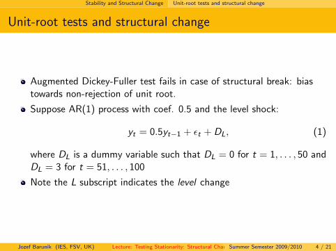
If the time series is Trend Stationary (TS), the tend is the mostimportant feature of the long-term behavior of that particular series.
So that knowing that time series is TS even with some structuralbreaks might have a great impact on forecasts (“predpoved” line onthe picture).Discussion about the U.S. GDP in Nelson-Plosser (1982), Perron(1989)...
Jozef Barunik (IES, FSV, UK) Lecture: Testing Stationarity: Structural Change ProblemSummer Semester 2009/2010 9 / 21
Stability and Structural Change Unit-root tests and structural change
Trend Stationarity and Structural Change
Jozef Barunik (IES, FSV, UK) Lecture: Testing Stationarity: Structural Change ProblemSummer Semester 2009/2010 10 / 21

Stability and Structural Change Unit-root tests and structural change
Unit-root tests and structural change
Simple approach to test stationarity in the presence of a structuralbreak is to split the time series to segments and test ADF on each ofthem
Caveats:
Loosing degrees of freedom (twice so high number of parameters).Prior knowledge about the break needed.
Perron’s test (Perron, 1989) solves these problems.
Jozef Barunik (IES, FSV, UK) Lecture: Testing Stationarity: Structural Change ProblemSummer Semester 2009/2010 11 / 21
Stability and Structural Change Perron’s test
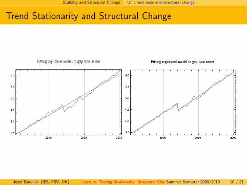
Perron’s test
Assume a structural change at time t = τ + 1.
Then,
H1 : yt = α0 + yt−1 + µ1DP + εt ,
A1 : yt = α0 + a2t + µ2DL + εt ,
where DP is pulse dummy such that DP = 1 if t = τ + 1 and zerootherwise.
and DL represents a level dummy such that DL = 1 if t > τ and zerootherwise.
Under the null H1, {yt} is a unit root process with one-time jump inthe level in period t = τ + 1
Under the alternative HA, {yt} is trend-stationary with a one jump inthe intercept.
Jozef Barunik (IES, FSV, UK) Lecture: Testing Stationarity: Structural Change ProblemSummer Semester 2009/2010 12 / 21

Stability and Structural Change Perron’s test
Perron’s test
Perron’s test thus allows to distinguish between difference stationarityand trend stationarity.
To test the H0 we need to estimate following equation:
yt = α0 + α1yt−1 + α2t + µ1DL + µ2DP +k∑
i=1
βi∆yt−i + εt , (2)
and compare the t-statistic for the null α1 = 1 with the critical valuesby Perron(1989):
Jozef Barunik (IES, FSV, UK) Lecture: Testing Stationarity: Structural Change ProblemSummer Semester 2009/2010 13 / 21
Stability and Structural Change Perron’s test
Perron’s test
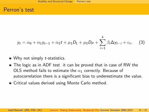
yt = α0 + α1yt−1 + α2t + µ1DL + µ2DP +k∑
i=1
βi∆yt−i + εt , (3)
Why not simply t-statistics.
The logic as in ADF test it can be proved that in case of RW theOLS method fails to estimate the α1 correctly. Because ofautocorrelation there is a significant bias to underestimate the value.
Critical values derived using Monte Carlo method.
Jozef Barunik (IES, FSV, UK) Lecture: Testing Stationarity: Structural Change ProblemSummer Semester 2009/2010 14 / 21
Stability and Structural Change Perron’s test
Perron’s test - Extensions
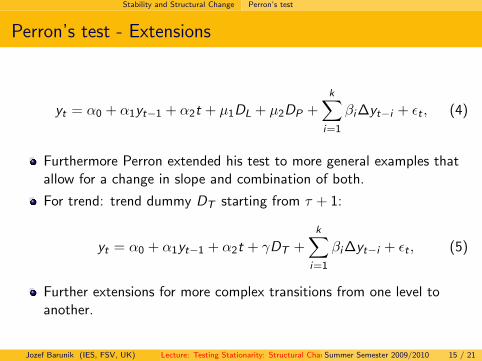
yt = α0 + α1yt−1 + α2t + µ1DL + µ2DP +k∑
i=1
βi∆yt−i + εt , (4)
Furthermore Perron extended his test to more general examples thatallow for a change in slope and combination of both.
For trend: trend dummy DT starting from τ + 1:
yt = α0 + α1yt−1 + α2t + γDT +k∑
i=1
βi∆yt−i + εt , (5)
Further extensions for more complex transitions from one level toanother.
Jozef Barunik (IES, FSV, UK) Lecture: Testing Stationarity: Structural Change ProblemSummer Semester 2009/2010 15 / 21

Stability and Structural Change U-R test
U-R test with structural breaks in JMulti
Slightly more advanced version following Lanne, Lutkepohl andSaikkonen (2002):
Deterministic part estimated via GLS, substracted from original seriesand the resulting series tested in a ADF test fashion.
Lanne et al. (2002) showed that their test performs better on smallsamples.
Again own critical values, reported in each test window.
Next slide shows types of the structural shift included in JMulti.
Jozef Barunik (IES, FSV, UK) Lecture: Testing Stationarity: Structural Change ProblemSummer Semester 2009/2010 16 / 21

Stability and Structural Change U-R test
Level shifts types in JMulti
Jozef Barunik (IES, FSV, UK) Lecture: Testing Stationarity: Structural Change ProblemSummer Semester 2009/2010 17 / 21

Stability and Structural Change U-R test
Level shifts types in JMulti
yt = α0 + α1ft(θ)γ + . . .
Exponential shift:t < τ . . . 0t ≥ τ . . . (1− exp(−θ(t − τ + 1)))
Rational shift:t < τ . . . 0, t = τ . . . γ1
t ≥ τ . . . (γ1 +∑T−τ
j=1 θi−1(θγ1 + γ2))
θ determines speed of the transition, the larger, the faster.
Next slide: some examples
Note that in Jmulti the break date means start of the transition, theJmulti functions are not centered as on the next picture.
Jozef Barunik (IES, FSV, UK) Lecture: Testing Stationarity: Structural Change ProblemSummer Semester 2009/2010 18 / 21

Stability and Structural Change U-R test
Level shifts types in JMulti
Jozef Barunik (IES, FSV, UK) Lecture: Testing Stationarity: Structural Change ProblemSummer Semester 2009/2010 19 / 21
Stability and Structural Change Conclusion
Conclusion
Distinction between Trend- and Difference- stationarity importantfor forecasting: the knowledge about trend is very valuable.
Sometimes the picture about the nature of stationarity is distorted bythe presence of structural breaks (the UR tests don’t work in thesecases).
Perron’s test solves this problem.
As in ADF critical values derived from Monte Carlo simulations.
This leads us to the more general question of stability, which isusually tested using the Chow Test. Another tests and differentperspectives will be presented during next lectures and seminars.
One problem connected with structural breaks: forecasting. Usuallystructural breaks become evident after some delay.
Jozef Barunik (IES, FSV, UK) Lecture: Testing Stationarity: Structural Change ProblemSummer Semester 2009/2010 20 / 21

Stability and Structural Change Conclusion
Examples during the Seminar
Thank you for your Attention !
Jozef Barunik (IES, FSV, UK) Lecture: Testing Stationarity: Structural Change ProblemSummer Semester 2009/2010 21 / 21