Lecture - Washington State Universityusers.tricity.wsu.edu/~hudson/Teaching/EE221/Text/06 3D plots and... · Lecture 6 3D plots and ... Both Scilab and Matlab use this convention

Lecture 63D plots and animation

1 IntroductionThe majority of graphing tasks we face are typically two-dimensional functions of the formy= f (x ) . However, not all functions have a single “input” and a single “output.” The motion of

a particle through space is described by vector position vs time

r (t)=[ x (t) , y (t ) , z (t )]

We could represent this by three 2D plots, but a more physical representation would be to tracethe particle trajectory in a single 3D plot. In this case the independent variable t does not formone of the plot axes. Instead it is a parameter of the motion. The resulting graph is called aparametric plot.

Some engineering problems deal with fields. A field is physical property which can varythroughout space. For example, the variation of ground elevation across a region of Earth'ssurface can be expressed as

z= f ( x , y)

Here the two coordinates x,y might correspond to longitude and latitude and z to groundelevation, possibly obtained from surveying. Or, z might represent surface temperature oratmospheric pressure. In those cases we might also be interested with variation through time aswell as through space.

Since a computer screen is two dimensional, plots in three (and higher) dimensions willnecessarily have to represent a single projection of the function. Different projections mighthighlight certain aspects of the function and obscure others. This problem grows with the numberof dimensions and is why scientific visualization is an active field of research.

In this lecture we want learn a few basic 3D plotting techniques. We will use the following code

Nx = 80;Ny = 40;x = linspace(-6,6,Nx);y = linspace(-3,3,Ny);z = zeros(Ny,Nx);for i=1:Nx for j=1:Ny z(j,i) = cos(x(i))*sin(y(j)); endend

to generate an array of z values which we will plot in various ways. Notice that the first index ofthe z array corresponds to the y coordinate and the second index to the x coordinate. This relatesto the raster scan format traditionally used on computer monitors and the way arrays appear ingraphics cards. Both Scilab and Matlab use this convention.

EE 221 Numerical Computing Scott Hudson 2016-01-08

Lecture 6: 3D plots and animation 2/9

2 The surf and mesh commandsGiven any 2D array of real numbers z either of the commands

surf(z);mesh(z);

will plot the z values as the elevation field of a 3D surface. The mesh command shows thissurface as a “wire mesh” while the surf command show it as a solid color-coded surface. The xand y coordinates are the integer indicies of the array. Alternately we can explicitly provide x andy values

surf(x,y,z);

The result for our data is shown in Fig. 3. Because this is a 2D projection of a 3D surface, someparts of the surface may be obscured. To get different views use the Rotation tool from the Toolsmenu. Click (right button in Scilab, left button in Matlab) and drag with your mouse to reorientthe surface. As in the 2D case, we can export a figure to a graphics file for inclusion in apresentation or paper.

2.1 Changing figure and axes properties interactively (Scilab)

As with 2D plots we can use the Edit => Figure properties menu option to change the appearanceof our figure. Similar options are available in Scilab and Matlab but the details differ. We willconsider Scilab.

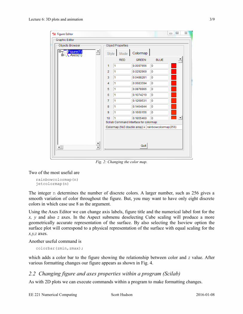
One of the most visually noticeable changes we can make is to use a different color map. Thecolor map specifies how different z values are mapped into different colors. This can be changedby either directly editing the red-green-blue values (Fig. 2) or more practically by specifying acolor map in the Colormap dialog box. Scilab has several predefined color maps (see helpcolormap).


Fig. 1: Output of surf(x,y,z) command


Two of the most useful are

rainbowcolormap(n)jetcolormap(n)

The integer n determines the number of discrete colors. A larger number, such as 256 gives asmooth variation of color throughout the figure. But, you may want to have only eight discretecolors in which case use 8 as the argument.

Using the Axes Editor we can change axis labels, figure title and the numerical label font for thex, y and also z axes. In the Aspect submenu deselecting Cube scaling will produce a moregeometrically accurate representation of the surface. By also selecting the Isoview option thesurface plot will correspond to a physical representation of the surface with equal scaling for thex,y,z axes.

Another useful command is

colorbar(zmin,zmax);

which adds a color bar to the figure showing the relationship between color and z value. Aftervarious formatting changes our figure appears as shown in Fig. 4.

2.2 Changing figure and axes properties within a program (Scilab)

As with 2D plots we can execute commands within a program to make formatting changes.


Fig. 2: Changing the color map.


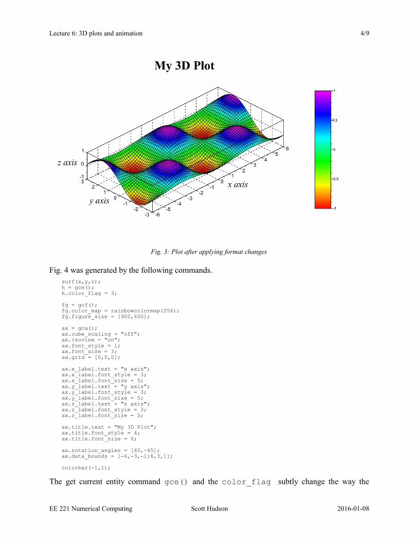
Fig. 4 was generated by the following commands.surf(x,y,z);h = gce();h.color_flag = 3;

fg = gcf();fg.color_map = rainbowcolormap(256);fg.figure_size = [900,600];

ax = gca();ax.cube_scaling = "off";ax.isoview = "on";ax.font_style = 1;ax.font_size = 3;ax.grid = [0,0,0];

ax.x_label.text = "x axis";ax.x_label.font_style = 3;ax.x_label.font_size = 5;ax.y_label.text = "y axis";ax.y_label.font_style = 3;ax.y_label.font_size = 5;ax.z_label.text = "z axis";ax.z_label.font_style = 3;ax.z_label.font_size = 5;

ax.title.text = "My 3D Plot";ax.title.font_style = 4;ax.title.font_size = 6;

ax.rotation_angles = [60,-45];ax.data_bounds = [-6,-3,-1;6,3,1];

colorbar(-1,1);

The get current entity command gce() and the color_flag subtly change the way the


Fig. 3: Plot after applying format changes


surface color is interpolated. You can experiment with flag values of 0 through 4. If you use thesecommands they must come immediately after the surf plotting command.

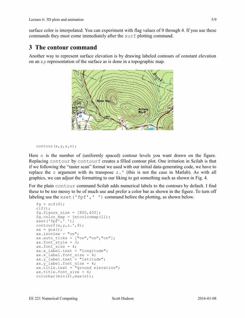
3 The contour commandAnother way to represent surface elevation is by drawing labeled contours of constant elevationon an x,y representation of the surface as is done in a topographic map.

contour(x,y,z,n);

Here n is the number of (uniformly spaced) contour levels you want drawn on the figure.Replacing contour by contourf creates a filled contour plot. One irritation in Scilab is thatif we following the “raster scan” format we used with our initial data-generating code, we have toreplace the z argument with its transpose z.' (this is not the case in Matlab). As with allgraphics, we can adjust the formatting to our liking to get something such as shown in Fig. 4.

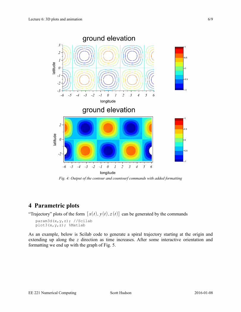
For the plain contour command Scilab adds numerical labels to the contours by default. I findthese to be too messy to be of much use and prefer a color bar as shown in the figure. To turn offlabeling use the xset('fpf',' ') command before the plotting, as shown below.

fg = scf(0);clf();fg.figure_size = [800,400];fg.color_map = jetcolormap(11);xset('fpf',' ');contourf(x,y,z.',9);ax = gca();ax.isoview = "on";ax.auto_ticks = ["on","on","on"];ax.font_style = 3;ax.font_size = 4;ax.x_label.text = "longitude";ax.x_label.font_size = 4;ax.y_label.text = "latitude";ax.y_label.font_size = 4;ax.title.text = "ground elevation";ax.title.font_size = 6;colorbar(min(z),max(z));



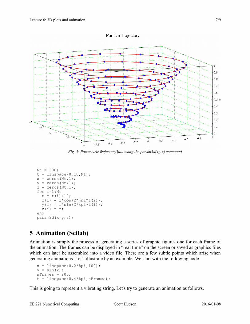
4 Parametric plots“Trajectory” plots of the form [ x( t) , y (t ) , z (t)] can be generated by the commands

param3d(x,y,z); //Scilabplot3(x,y,z); %Matlab

As an example, below is Scilab code to generate a spiral trajectory starting at the origin andextending up along the z direction as time increases. After some interactive orientation andformatting we end up with the graph of Fig. 5.


Fig. 4: Output of the contour and countourf commands with added formatting


Nt = 200;t = linspace(0,10,Nt);x = zeros(Nt,1);y = zeros(Nt,1);z = zeros(Nt,1);for i=1:Nt r = t(i)/10; x(i) = r*cos(2*%pi*t(i)); y(i) = r*sin(2*%pi*t(i)); z(i) = r;endparam3d(x,y,z);

5 Animation (Scilab)Animation is simply the process of generating a series of graphic figures one for each frame ofthe animation. The frames can be displayed in “real time” on the screen or saved as graphics fileswhich can later be assembled into a video file. There are a few subtle points which arise whengenerating animations. Let's illustrate by an example. We start with the following code

x = linspace(0,2*%pi,100);y = sin(x);nFrames = 200;t = linspace(0,4*%pi,nFrames);

This is going to represent a vibrating string. Let's try to generate an animation as follows.


Fig. 5: Parametric "trajectory" plot using the param3d(x,y,z) command


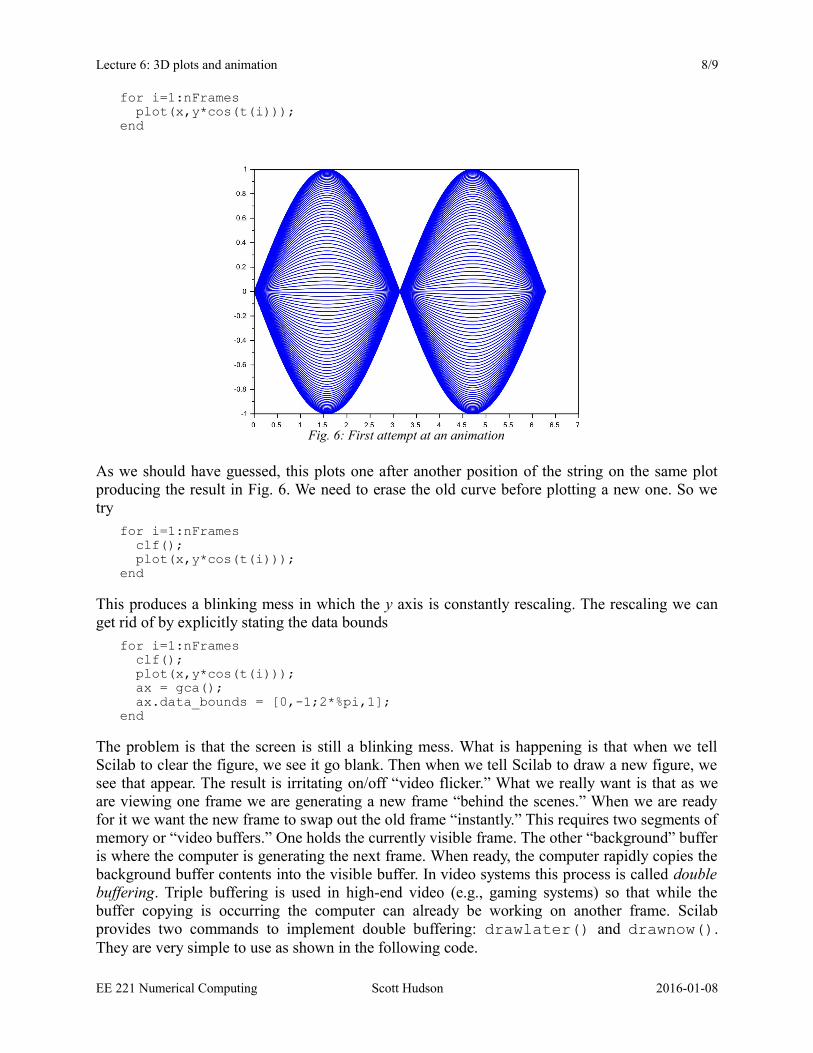
for i=1:nFrames plot(x,y*cos(t(i)));end

As we should have guessed, this plots one after another position of the string on the same plotproducing the result in Fig. 6. We need to erase the old curve before plotting a new one. So wetry

for i=1:nFrames clf(); plot(x,y*cos(t(i)));end

This produces a blinking mess in which the y axis is constantly rescaling. The rescaling we canget rid of by explicitly stating the data bounds

for i=1:nFrames clf(); plot(x,y*cos(t(i))); ax = gca(); ax.data_bounds = [0,-1;2*%pi,1];end

The problem is that the screen is still a blinking mess. What is happening is that when we tellScilab to clear the figure, we see it go blank. Then when we tell Scilab to draw a new figure, wesee that appear. The result is irritating on/off “video flicker.” What we really want is that as weare viewing one frame we are generating a new frame “behind the scenes.” When we are readyfor it we want the new frame to swap out the old frame “instantly.” This requires two segments ofmemory or “video buffers.” One holds the currently visible frame. The other “background” bufferis where the computer is generating the next frame. When ready, the computer rapidly copies thebackground buffer contents into the visible buffer. In video systems this process is called doublebuffering. Triple buffering is used in high-end video (e.g., gaming systems) so that while thebuffer copying is occurring the computer can already be working on another frame. Scilabprovides two commands to implement double buffering: drawlater() and drawnow().They are very simple to use as shown in the following code.


Fig. 6: First attempt at an animation


for i=1:nFrames drawlater(); //turn on double buffering so that operations clf(); //occur in the background plot(x,y*cos(t(i))); ax = gca(); ax.data_bounds = [0,-1;2*%pi,1]; drawnow(); //copy the background buffer to the visible bufferend

This solves our problems. Inbetween the drawlater() and drawnow() commands we canmodify the figure in anyway we wish – adding labels, titles, changing color maps and so on.

The speed with which frames update depends on how long it takes to generate a new frame. If thegoal is to produce an independent video file then we want to save each frame to disk. Oneapproach is shown here.

scf(0);for i=1:nFrames drawlater();

//generate a new frame here

drawnow(); fname = msprintf("frames/f%03d.png",i); while (~isfile(fname)) xs2png(0,fname); endend

First we create a subdirectory names “frames” before running the animation code. During theanimation rendering the msprintf function creates a series of file names from the frame indexi. If this png file does not already exist it is written from the current graphics frame. The result isa sequence of png files

f001.png , f002.png , ...

in the subdirectory frames. From there video editing software can be used to produce ananimation file. A useful free and open-source program for this is Virtualdub (virtualdub.org).


Documents

Lecture - Washington State Universityusers.tricity.wsu.edu/~hudson/Teaching/EE221/Text/06 3D plots and... · Lecture 6 3D plots and ... Both Scilab and Matlab use this convention