Lecture3 Optimal Risky Portfolios

8/3/2019 Lecture3 Optimal Risky Portfolios

http://slidepdf.com/reader/full/lecture3-optimal-risky-portfolios 1/21

The Optimal Risky Portfolio

Lecture No.3² SAPM



Portfolio construction Process

Capital allocation between risky portfolio and risk-free

assets

± Depends upon risk aversion and risk-return trade-off

Asset allocation among asset classes

± Broad outlines of portfolio established

Security selection

± Specific securities selected for the portfolio

Steps 2 and 3 lead to optimal risky portfolio

Optimal risky portfolio is the combination of risky assets that

provides the best risk-return trade-off



Diversification and portfolio risk

Two sources of risk ²

± firm-specific risk or unique risk

± Market risk or systematic risk (inflation, business cycles,

exchange rates etc )

Diversification can reduce firm-specific risk to zero if

specific risk is independent ( known as the insurance principle)

Diversification cannot eliminate the systematic risk, i.e. risk

attributable to market-wide sources

Hence investors only care about systematic risks

Return on assets compensates only for systematic risks



Portfolio expected return and risk

Consider 2 risky assets, a debt mutual fund D and an equity

mutual fund E

If the weights of the 2 assets are Wd and We then portfolio

expected return E(rp) is

and portfolio risk (p) is given as



Correlation and Portfolio Risk Expected return of the portfolio is the weighted average of

expected returns of component assets with their proportions as

weights

Portfolio variance is driven by the covariance between

component assets If correlation between assets is 1 (perfect positive correlation)

then portfolio standard deviation = weighted average of

component standard deviations

If correlation less than 1, portfolio standard deviation islessthan weighted average of component standard deviations

If correlation is -1 (perfect negative correlation), portfolio

variance is lowest ² we can construct a zero-variance portfolio



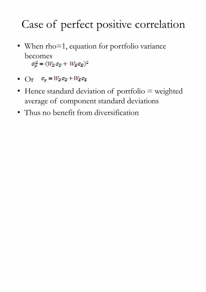
Case of perfect positive correlation

When rho=1, equation for portfolio variance

becomes

Or

Hence standard deviation of portfolio = weighted

average of component standard deviations

Thus no benefit from diversification



Correlation > 0 < 1

When assets are less than perfectly positively correlated

we can construct the minimum variance portfolio

The Minimum Variance Portfolio has a standard

deviation less than that of the component assets Equation for obtaining weights for Minimum Variance

Portfolio for portfolio consisting of 2 assets D and E

Example



When correlation is zero

The equation for portfolio variance becomes

The weights for the minimum variance portfolio

are

and



Case of perfect negative correlation

For assets with perfect negative correlation

The weights for the zero variance portfolio are

and



Example-Portfolio return and risk

The expected return and risk of the two assets are E(rd)= 0.08,

E(re)=0.13, (d) =0.12 and (e)=0.20

Wd We E( rp) Portfolio Std Deviation for the gi ven correl ation

-1 0 0.3 1

0.00 1.00 0.1300 0.2000 0.2000 0.2000 0.2000

0.10 0.90 0.1250 0.1680 0.1804 0.1840 0.1920

0.20 0.80 0.1200 0.1360 0.1618 0.1688 0.1840

0.30 0.70 0.1150 0.1040 0.1446 0.1547 0.1760

0.40 0.60 0.1100 0.0720 0.1292 0.1420 0.1680

0.50 0.50 0.1050 0.0400 0.1166 0.1311 0.1600

0.60 0.40 0.1000 0.0080 0.1076 0.1226 0.1520

0.70 0.30 0.0950 0.0240 0.1032 0.1170 0.1440

0.80 0.20 0.0900 0.0560 0.1040 0.1145 0.1360

0.90 0.10 0.0850 0.0880 0.1098 0.1156 0.1280

1.00 0.00 0.0800 0.1200 0.1200 0.1200 0.1200



Observations

For =1, portfolio standard deviation is simply weighted average

of asset standard deviation (no benefit of diversification)

For =0.30 and =0, portfolio standard deviation

± decreases initially as equity component increases indicating

diversification benefit and

± increases as portfolio becomes concentrated in equity

± we can find the minimum-variance portfolio which has

standard deviation less than that of individual assets

For =-1, diversification is most effective due to ´perfect hedgeµ

± For =-1, we can construct a zero-variance portfolio



Portfolio expected return and SD

Exhibit 4.5: Mean Standard Deviation Diagram: Portfolios of Two Risky Securities with

Arbitrary Correlation, V



The Minimum Variance Frontier

We plot the set of portfolios with the lowest variance at a given

level of expected return ( recall the mean variance criterion)

Above set known as the Mean Standard Deviation frontier or

Minimum Variance frontier Portion of mean-SD frontier below the global minimum variance

portfolio is inefficient

For each frontier portfolio on the lower portion there exists

another frontier portfolio on the upper portion with same but a

higher E(r)

Portion above the global minimum variance portfolio is known as

the efficient frontier in the absence of a risk-free asset

Investors will only choose a portfolio on the efficient frontier



The Efficient Frontier



Risky Portfolio with a risk-free asset Given a risky portfolio of 2 risky assets, a debt mutual fund and

an equity mutual fund and a risk-free asset with return rf

How do we find the optimal risky portfolio?

Plot CALs starting from the risk-free rate and passing through

the opportunity set of risky assets ² debt and equity funds

The highest CAL will have highest slope, i.e.Max S = (E(rp)-

rf)/p

Optimal risky portfolio is the tangency point of the highest CAL

to the portfolio opportunity set Tangency portfolio consists of risky assets only



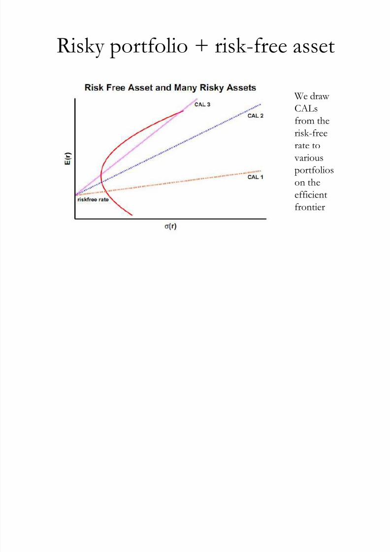
Risky portfolio + risk-free asset

We draw

CALs

from the

risk-freerate to

various

portfolios

on the

efficient

frontier



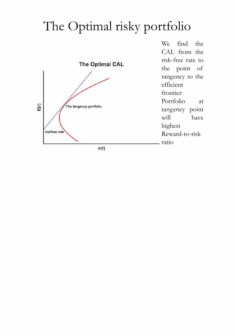
The Optimal risky portfolio

We find theCAL from the

risk-free rate to

the point of

tangency to the

efficientfrontier

Portfolio at

tangency point

will have

highestReward-to-risk

ratio



Optimal Risky Portfolio ² 2 assets

Equation for determining weights of optimal risky portfolio with

2 risky assets

And

where RD and RE are excess returns on debt and equity funds

i.e. Expected return less the risk-free rate



Optimal Complete Portfolio

Calculate the weights of the optimal risky portfolio as

above

Compute the E(r ) and of the optimal risky portfolio

We have the risk-free rate and the investor·s degree of

risk aversion

Proportion to be invested in risky portfolio is

Balance is the proportion invested in risk-free asset



Optimal Complete Portfolio

Point P where the

CAL is tangent to

the efficient frontier

depicts the optimal

risky portfolio At Points 1 and 2

the indifference

curves of 2 different

investors are tangent

to the CAL

Points 1 and 2depict the

O ptimum

com plete portfolio

for those investors



Summary

Note that optimal risky portfolio is the same for all investors

± F ormula for computation of weights of optimal risky portfolio does not

include the investor·s degree of risk aversion

Hence the fund manager will offer the same optimal risky portfolio

to all his investors- his job becomes easier !

The optimal com plete portfolio for each investor (the allocation

of funds between the risky portion and risk-free portion) will be

different

It will depend on investor·s preferences, i.e. his degree of risk aversion and indifference curve

More risk averse investors will have lower proportion of the

optimal risky portfolio in their complete portfolio than less risk-

averse investors

Documents

Lecture3 Optimal Risky Portfolios