Lecture’Notesfor’Chapter’2 Introduction’to…kumar001/dmbook/slides/chap2_data… · 01/22/2018 Introduction/ toDataMining,2nd/Edition 1 Data$Mining:$Data Lecture’Notesfor’Chapter’2

01/22/2018 1Introduction to Data Mining, 2nd Edition

Data Mining: Data

Lecture Notes for Chapter 2

Introduction to Data Mining , 2nd Editionby

Tan, Steinbach, Karpatne, Kumar


Outline

Attributes and Objects

Types of Data

Data Quality

Similarity and Distance

Data Preprocessing

What is Data?

Collection of data objects and their attributes

An attribute is a property or characteristic of an object– Examples: eye color of a person, temperature, etc.

– Attribute is also known as variable, field, characteristic, dimension, or feature

A collection of attributes describe an object– Object is also known as record, point, case, sample, entity, or instance

Tid Refund Marital Status

Taxable Income Cheat

1 Yes Single 125K No

2 No Married 100K No

3 No Single 70K No

4 Yes Married 120K No

5 No Divorced 95K Yes

6 No Married 60K No

7 Yes Divorced 220K No

8 No Single 85K Yes

9 No Married 75K No

10 No Single 90K Yes 10

Attributes

Objects


A More Complete View of Data

Data may have parts

The different parts of the data may have relationships

More generally, data may have structure

Data can be incomplete

We will discuss this in more detail later


Attribute Values

Attribute values are numbers or symbols assigned to an attribute for a particular object

Distinction between attributes and attribute values– Same attribute can be mapped to different attribute valuesu Example: height can be measured in feet or meters

– Different attributes can be mapped to the same set of valuesu Example: Attribute values for ID and age are integersu But properties of attribute values can be different

Measurement of Length The way you measure an attribute may not match the attributes properties.

1

2

3

5

5

7

8

15

10 4

A

B

C

D

E

This scale preserves the ordering and additvity properties of length.

This scale preserves only the ordering property of length.


Types of Attributes

There are different types of attributes– Nominal

u Examples: ID numbers, eye color, zip codes– Ordinal

u Examples: rankings (e.g., taste of potato chips on a scale from 1-10), grades, height tall, medium, short

– Intervalu Examples: calendar dates, temperatures in Celsius or Fahrenheit.

– Ratiou Examples: temperature in Kelvin, length, time, counts


Properties of Attribute Values

The type of an attribute depends on which of the following properties/operations it possesses:– Distinctness: = ≠– Order: < >– Differences are + -meaningful :

– Ratios are * /meaningful

– Nominal attribute: distinctness– Ordinal attribute: distinctness & order– Interval attribute: distinctness, order & meaningful differences

– Ratio attribute: all 4 properties/operations


Difference Between Ratio and Interval

Is it physically meaningful to say that a temperature of 10 ° is twice that of 5° on – the Celsius scale?– the Fahrenheit scale?– the Kelvin scale?

Consider measuring the height above average– If Bill’s height is three inches above average and Bob’s height is six inches above average, then would we say that Bob is twice as tall as Bill?

– Is this situation analogous to that of temperature?

Attribute Type

Description

Examples

Operations

Nominal

Nominal attribute values only distinguish. (=, ≠)

zip codes, employee ID numbers, eye color, sex: male, female

mode, entropy, contingency correlation, χ2 test

Categorical

Qualitative

Ordinal Ordinal attribute values also order objects. (<, >)

hardness of minerals, good, better, best, grades, street numbers

median, percentiles, rank correlation, run tests, sign tests

Interval For interval attributes, differences between values are meaningful. (+, - )

calendar dates, temperature in Celsius or Fahrenheit

mean, standard deviation, Pearson's correlation, t and F tests

Numeric

Quantitative

Ratio For ratio variables, both differences and ratios are meaningful. (*, /)

temperature in Kelvin, monetary quantities, counts, age, mass, length, current

geometric mean, harmonic mean, percent variation

This categorization of attributes is due to S. S. Stevens

Attribute Type

Transformation

Comments

Categorical

Qualitative

Nominal

Any permutation of values

If all employee ID numbers were reassigned, would it make any difference?

Ordinal An order preserving change of values, i.e., new_value = f(old_value) where f is a monotonic function

An attribute encompassing the notion of good, better best can be represented equally well by the values 1, 2, 3 or by 0.5, 1, 10.

Numeric

Quantitative

Interval new_value = a * old_value + b where a and b are constants

Thus, the Fahrenheit and Celsius temperature scales differ in terms of where their zero value is and the size of a unit (degree).

Ratio new_value = a * old_value

Length can be measured in meters or feet.

This categorization of attributes is due to S. S. Stevens


Discrete and Continuous Attributes

Discrete Attribute– Has only a finite or countably infinite set of values– Examples: zip codes, counts, or the set of words in a collection of documents

– Often represented as integer variables. – Note: binary attributes are a special case of discrete attributes

Continuous Attribute – Has real numbers as attribute values– Examples: temperature, height, or weight. – Practically, real values can only be measured and represented using a finite number of digits.

– Continuous attributes are typically represented as floating-point variables.


Asymmetric Attributes Only presence (a non-zero attribute value) is regarded as important

u Words present in documentsu Items present in customer transactions

If we met a friend in the grocery store would we ever say the following?“I see our purchases are very similar since we didn’t buy most of the same things.”

We need two asymmetric binary attributes to represent one ordinary binary attribute– Association analysis uses asymmetric attributes

Asymmetric attributes typically arise from objects that are sets


Some Extensions and Critiques

Velleman, Paul F., and Leland Wilkinson. "Nominal, ordinal, interval, and ratio typologies are misleading."The American Statistician 47, no. 1 (1993): 65-72.

Mosteller, Frederick, and John W. Tukey. "Data analysis and regression. A second course in statistics." Addison-Wesley Series in Behavioral Science: Quantitative Methods, Reading, Mass.: Addison-Wesley, 1977.

Chrisman, Nicholas R. "Rethinking levels of measurement for cartography."Cartography and Geographic Information Systems 25, no. 4 (1998): 231-242.


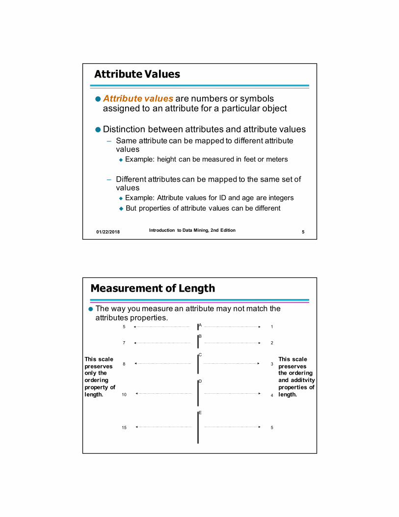
Critiques

Incomplete – Asymmetric binary– Cyclical– Multivariate– Partially ordered– Partial membership– Relationships between the data

Real data is approximate and noisy– This can complicate recognition of the proper attribute type– Treating one attribute type as another may be approximately correct


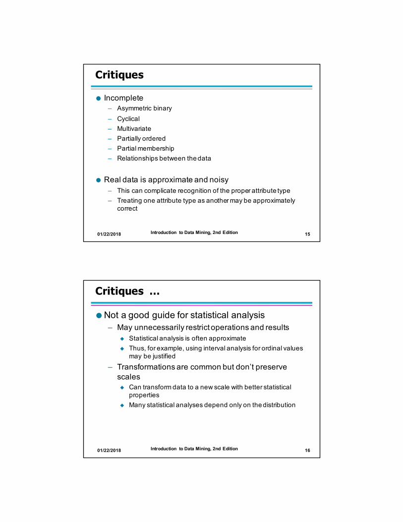
Critiques …

Not a good guide for statistical analysis– May unnecessarily restrict operations and results

u Statistical analysis is often approximateu Thus, for example, using interval analysis for ordinal values may be justified

– Transformations are common but don’t preserve scalesu Can transform data to a new scale with better statistical properties

u Many statistical analyses depend only on the distribution


More Complicated Examples

ID numbers – Nominal, ordinal, or interval?

Number of cylinders in an automobile engine – Nominal, ordinal, or ratio?

Biased Scale – Interval or Ratio


Key Messages for Attribute Types

The types of operations you choose should be “meaningful” for the type of data you have– Distinctness, order, meaningful intervals, and meaningful ratios are only four properties of data

– The data type you see – often numbers or strings – may not capture all the properties or may suggest properties that are not there

– Analysis may depend on these other properties of the datau Many statistical analyses depend only on the distribution

– Many times what is meaningful is measured by statistical significance

– But in the end, what is meaningful is measured by the domain


Types of data sets Record– Data Matrix– Document Data– Transaction Data

Graph– World Wide Web– Molecular Structures

Ordered– Spatial Data– Temporal Data– Sequential Data– Genetic Sequence Data


Important Characteristics of Data

– Dimensionality (number of attributes)u High dimensional data brings a number of challenges

– Sparsityu Only presence counts

– Resolutionu Patterns depend on the scale

– Sizeu Type of analysis may depend on size of data


Record Data

Data that consists of a collection of records, each of which consists of a fixed set of attributes

Tid Refund Marital Status

Taxable Income Cheat

1 Yes Single 125K No

2 No Married 100K No

3 No Single 70K No

4 Yes Married 120K No

5 No Divorced 95K Yes

6 No Married 60K No

7 Yes Divorced 220K No

8 No Single 85K Yes

9 No Married 75K No

10 No Single 90K Yes 10


Data Matrix

If data objects have the same fixed set of numeric attributes, then the data objects can be thought of as points in a multi-dimensional space, where each dimension represents a distinct attribute

Such data set can be represented by an m by n matrix, where there are m rows, one for each object, and ncolumns, one for each attribute

1.12.216.226.2512.65

1.22.715.225.2710.23

Thickness LoadDistanceProjection of y load

Projection of x Load

1.12.216.226.2512.65

1.22.715.225.2710.23

Thickness LoadDistanceProjection of y load

Projection of x Load


Document Data

Each document becomes a ‘term’ vector – Each term is a component (attribute) of the vector– The value of each component is the number of times the corresponding term occurs in the document.

Document 1

season

timeout

lost

win

game

score

ball

play

coach

team

Document 2

Document 3

3 0 5 0 2 6 0 2 0 2

0

0

7 0 2 1 0 0 3 0 0

1 0 0 1 2 2 0 3 0


Transaction Data

A special type of record data, where – Each record (transaction) involves a set of items. – For example, consider a grocery store. The set of products purchased by a customer during one shopping trip constitute a transaction, while the individual products that were purchased are the items.

TID Items

1 Bread, Coke, Milk

2 Beer, Bread

3 Beer, Coke, Diaper, Milk

4 Beer, Bread, Diaper, Milk

5 Coke, Diaper, Milk


Graph Data

Examples: Generic graph, a molecule, and webpages

5

2

1 25

Benzene Molecule: C6H6


Ordered Data

Sequences of transactions

An element of the sequence

Items/Events


Ordered Data

Genomic sequence data

GGTTCCGCCTTCAGCCCCGCGCCCGCAGGGCCCGCCCCGCGCCGTCGAGAAGGGCCCGCCTGGCGGGCGGGGGGAGGCGGGGCCGCCCGAGCCCAACCGAGTCCGACCAGGTGCCCCCTCTGCTCGGCCTAGACCTGAGCTCATTAGGCGGCAGCGGACAGGCCAAGTAGAACACGCGAAGCGCTGGGCTGCCTGCTGCGACCAGGG


Ordered Data

Spatio-Temporal Data

Average Monthly Temperature of land and ocean


Data Quality

Poor data quality negatively affects many data processing efforts

“The most important point is that poor data quality is an unfolding disaster.– Poor data quality costs the typical company at least ten

percent (10%) of revenue; twenty percent (20%) is probably a better estimate.”

Thomas C. Redman, DM Review, August 2004

Data mining example: a classification model for detecting people who are loan risks is built using poor data– Some credit-worthy candidates are denied loans– More loans are given to individuals that default


Data Quality …

What kinds of data quality problems? How can we detect problems with the data? What can we do about these problems?

Examples of data quality problems: – Noise and outliers – Missing values – Duplicate data – Wrong data


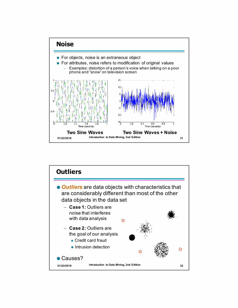
Noise

For objects, noise is an extraneous object For attributes, noise refers to modification of original values

– Examples: distortion of a person’s voice when talking on a poor phone and “snow” on television screen

Two Sine Waves Two Sine Waves + Noise


Outliers are data objects with characteristics that are considerably different than most of the other data objects in the data set– Case 1: Outliers are noise that interfereswith data analysis

– Case 2: Outliers are the goal of our analysisu Credit card fraudu Intrusion detection

Causes?

Outliers


Missing Values

Reasons for missing values– Information is not collected (e.g., people decline to give their age and weight)

– Attributes may not be applicable to all cases (e.g., annual income is not applicable to children)

Handling missing values– Eliminate data objects or variables– Estimate missing values

u Example: time series of temperatureu Example: census results

– Ignore the missing value during analysis


Missing Values …

Missing completely at random (MCAR)– Missingness of a value is independent of attributes– Fill in values based on the attribute– Analysis may be unbiased overall

Missing at Random (MAR)– Missingness is related to other variables– Fill in values based other values– Almost always produces a bias in the analysis

Missing Not at Random (MNAR)– Missingness is related to unobserved measurements– Informative or non-ignorable missingness

Not possible to know the situation from the data


Duplicate Data

Data set may include data objects that are duplicates, or almost duplicates of one another– Major issue when merging data from heterogeneous sources

Examples:– Same person with multiple email addresses

Data cleaning– Process of dealing with duplicate data issues

When should duplicate data not be removed?


Similarity and Dissimilarity Measures

Similarity measure– Numerical measure of how alike two data objects are.– Is higher when objects are more alike.– Often falls in the range [0,1]

Dissimilarity measure– Numerical measure of how different two data objects are

– Lower when objects are more alike– Minimum dissimilarity is often 0– Upper limit varies

Proximity refers to a similarity or dissimilarity


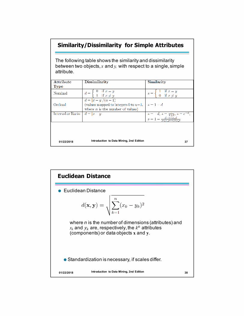
Similarity/Dissimilarity for Simple Attributes

The following table shows the similarity and dissimilarity between two objects, x and y, with respect to a single, simple attribute.


Euclidean Distance

Euclidean Distance

where n is the number of dimensions (attributes) and xk and yk are, respectively, the kth attributes (components) or data objects x and y.

Standardization is necessary, if scales differ.


Euclidean Distance

0

1

2

3

0 1 2 3 4 5 6

p1

p2

p3 p4

point x yp1 0 2p2 2 0p3 3 1p4 5 1

Distance Matrix

p1 p2 p3 p4p1 0 2.828 3.162 5.099p2 2.828 0 1.414 3.162p3 3.162 1.414 0 2p4 5.099 3.162 2 0


Minkowski Distance

Minkowski Distance is a generalization of Euclidean Distance

Where r is a parameter, n is the number of dimensions (attributes) and xk and yk are, respectively, the kth

attributes (components) or data objects x and y.


Minkowski Distance: Examples

r = 1. City block (Manhattan, taxicab, L1 norm) distance. – A common example of this is the Hamming distance, which is just the number of bits that are different between two binary vectors

r = 2. Euclidean distance

r→ ∞. “supremum” (Lmax norm, L∞ norm) distance. – This is the maximum difference between any component of the vectors

Do not confuse r with n, i.e., all these distances are defined for all numbers of dimensions.


Minkowski Distance

Distance Matrix

point x yp1 0 2p2 2 0p3 3 1p4 5 1

L1 p1 p2 p3 p4p1 0 4 4 6p2 4 0 2 4p3 4 2 0 2p4 6 4 2 0

L2 p1 p2 p3 p4p1 0 2.828 3.162 5.099p2 2.828 0 1.414 3.162p3 3.162 1.414 0 2p4 5.099 3.162 2 0

L∞ p1 p2 p3 p4p1 0 2 3 5p2 2 0 1 3p3 3 1 0 2p4 5 3 2 0


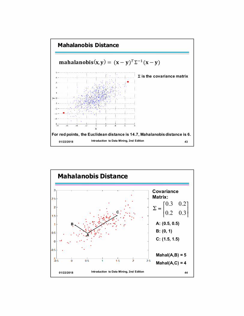
Mahalanobis Distance

For red points, the Euclidean distance is 14.7, Mahalanobis distance is 6.

Σ is the covariance matrix

𝐦𝐚𝐡𝐚𝐥𝐚𝐧𝐨𝐛𝐢𝐬 𝐱, 𝐲 = (𝐱 − 𝐲)4Ʃ67(𝐱 − 𝐲)


Mahalanobis Distance

Covariance Matrix:

⎥⎦

⎤⎢⎣

⎡=Σ

3.02.02.03.0

A: (0.5, 0.5)B: (0, 1)

C: (1.5, 1.5)

Mahal(A,B) = 5

Mahal(A,C) = 4

B

A

C


Common Properties of a Distance

Distances, such as the Euclidean distance, have some well known properties.

1. d(x, y) ≥ 0 for all x and y and d(x, y) = 0 only if x = y. (Positive definiteness)

2. d(x, y) = d(y, x) for all x and y. (Symmetry)3. d(x, z) ≤ d(x, y) + d(y, z) for all points x, y, and z.

(Triangle Inequality)

where d(x, y) is the distance (dissimilarity) between points (data objects), x and y.

A distance that satisfies these properties is a metric


Common Properties of a Similarity

Similarities, also have some well known properties.

1. s(x, y) = 1 (or maximum similarity) only if x = y.

2. s(x, y) = s(y, x) for all x and y. (Symmetry)

where s(x, y) is the similarity between points (data objects), x and y.


Similarity Between Binary Vectors

Common situation is that objects, p and q, have only binary attributes

Compute similarities using the following quantitiesf01 = the number of attributes where p was 0 and q was 1f10 = the number of attributes where p was 1 and q was 0f00 = the number of attributes where p was 0 and q was 0f11 = the number of attributes where p was 1 and q was 1

Simple Matching and Jaccard Coefficients SMC = number of matches / number of attributes

= (f11 + f00) / (f01 + f10 + f11 + f00)

J = number of 11 matches / number of non-zero attributes= (f11) / (f01 + f10 + f11)


SMC versus Jaccard: Example

x = 1 0 0 0 0 0 0 0 0 0 y = 0 0 0 0 0 0 1 0 0 1

f01 = 2 (the number of attributes where p was 0 and q was 1)f10 = 1 (the number of attributes where p was 1 and q was 0)f00 = 7 (the number of attributes where p was 0 and q was 0)f11 = 0 (the number of attributes where p was 1 and q was 1)

SMC = (f11 + f00) / (f01 + f10 + f11 + f00)= (0+7) / (2+1+0+7) = 0.7

J = (f11) / (f01 + f10 + f11) = 0 / (2 + 1 + 0) = 0


Cosine Similarity

If d1 and d2 are two documentvectors, thencos( d1, d2 ) = <d1,d2> / ||d1|| ||d2|| ,

where <d1,d2> indicates inner product or vector dotproduct of vectors, d1 and d2, and || d || is the length ofvector d.

Example:d1 = 3 2 0 5 0 0 0 2 0 0

d2 = 1 0 0 0 0 0 0 1 0 2<d1, d2> = 3*1 + 2*0 + 0*0 + 5*0 + 0*0 + 0*0 + 0*0 + 2*1 + 0*0 + 0*2 = 5

| d1 || = (3*3+2*2+0*0+5*5+0*0+0*0+0*0+2*2+0*0+0*0)0.5 = (42) 0.5 = 6.481

|| d2 || = (1*1+0*0+0*0+0*0+0*0+0*0+0*0+1*1+0*0+2*2) 0.5 = (6) 0.5 = 2.449

cos(d1, d2 ) = 0.3150


Extended Jaccard Coefficient (Tanimoto)

Variation of Jaccard for continuous or count attributes– Reduces to Jaccard for binary attributes


Correlation measures the linear relationship between objects


Visually Evaluating Correlation

Scatter plots showing the similarity from –1 to 1.


Drawback of Correlation

x = (-3, -2, -1, 0, 1, 2, 3) y = (9, 4, 1, 0, 1, 4, 9)

yi = xi2

mean(x) = 0, mean(y) = 4 std(x) = 2.16, std(y) = 3.74

corr = (-3)(5)+(-2)(0)+(-1)(-3)+(0)(-4)+(1)(-3)+(2)(0)+3(5) / ( 6 * 2.16 * 3.74 )= 0


Comparison of Proximity Measures

Domain of application– Similarity measures tend to be specific to the type of attribute and data

– Record data, images, graphs, sequences, 3D-protein structure, etc. tend to have different measures

However, one can talk about various properties that you would like a proximity measure to have– Symmetry is a common one– Tolerance to noise and outliers is another– Ability to find more types of patterns? – Many others possible

The measure must be applicable to the data and produce results that agree with domain knowledge


Information Based Measures

Information theory is a well-developed and fundamental disciple with broad applications

Some similarity measures are based on information theory – Mutual information in various versions– Maximal Information Coefficient (MIC) and related measures

– General and can handle non-linear relationships– Can be complicated and time intensive to compute


Information and Probability

Information relates to possible outcomes of an event – transmission of a message, flip of a coin, or measurement of a piece of data

The more certain an outcome, the less information that it contains and vice-versa– For example, if a coin has two heads, then an outcome of heads provides no information

– More quantitatively, the information is related the probability of an outcomeu The smaller the probability of an outcome, the more information it provides and vice-versa

– Entropy is the commonly used measure


Entropy

For – a variable (event), X, – with n possible values (outcomes), x1, x2 …, xn

– each outcome having probability, p1, p2 …, pn

– the entropy of X , H(X), is given by

𝐻 𝑋 = −:𝑝<log@𝑝<

A

< B7

Entropy is between 0 and log2n and is measured in bits– Thus, entropy is a measure of how many bits it takes to represent an observation of X on average


Entropy Examples

For a coin with probability p of heads and probability q = 1 – p of tails

𝐻 = −𝑝 log@ 𝑝 − 𝑞 log@ 𝑞

– For p= 0.5, q = 0.5 (fair coin) H = 1– For p = 1 or q = 1, H = 0

What is the entropy of a fair four-sided die?


Entropy for Sample Data: Example

Maximum entropy is log25 = 2.3219

Hair Color Count p -plog2pBlack 75 0.75 0.3113Brown 15 0.15 0.4105Blond 5 0.05 0.2161Red 0 0.00 0Other 5 0.05 0.2161Total 100 1.0 1.1540


Entropy for Sample Data

Suppose we have – a number of observations (m) of some attribute, X, e.g., the hair color of students in the class,

– where there are n different possible values– And the number of observation in the ith category is mi

– Then, for this sample

𝐻 𝑋 = −:𝑚<

𝑚 log@𝑚<

𝑚

A

<B7

For continuous data, the calculation is harder


Mutual Information

Information one variable provides about another

Formally, 𝐼 𝑋,𝑌 = 𝐻 𝑋 +𝐻 𝑌 −𝐻(𝑋,𝑌), where

H(X,Y) is the joint entropy of X and Y,

𝐻 𝑋, 𝑌 = −::𝑝𝑖𝑗log@ 𝑝𝑖𝑗J<

Where pij is the probability that the ith value of X and the jth value of Yoccur together

For discrete variables, this is easy to compute

Maximum mutual information for discrete variables is log2(min( nX, nY ), where nX (nY) is the number of values of X (Y)


Mutual Information Example

Student Status

Count p -plog2p

Undergrad 45 0.45 0.5184

Grad 55 0.55 0.4744

Total 100 1.00 0.9928

Grade Count p -plog2pA 35 0.35 0.5301

B 50 0.50 0.5000

C 15 0.15 0.4105

Total 100 1.00 1.4406

Student Status

Grade Count p -plog2p

Undergrad A 5 0.05 0.2161

Undergrad B 30 0.30 0.5211

Undergrad C 10 0.10 0.3322

Grad A 30 0.30 0.5211

Grad B 20 0.20 0.4644

Grad C 5 0.05 0.2161

Total 100 1.00 2.2710

Mutual information of Student Status and Grade = 0.9928 + 1.4406 - 2.2710 = 0.1624


Maximal Information Coefficient

Reshef, David N., Yakir A. Reshef, Hilary K. Finucane, Sharon R. Grossman, Gilean McVean, Peter J. Turnbaugh, Eric S. Lander, Michael Mitzenmacher, and Pardis C. Sabeti. "Detecting novel associations in large data sets." science 334, no. 6062 (2011): 1518-1524.

Applies mutual information to two continuous variables

Consider the possible binnings of the variables into discrete categories– nX × nY ≤ N0.6where

u nX is the number of values of Xu nY is the number of values of Yu N is the number of samples (observations, data objects)

Compute the mutual information– Normalized by log2(min( nX, nY )

Take the highest value


General Approach for Combining Similarities

Sometimes attributes are of many different types, but an overall similarity is needed.

1: For the kth attribute, compute a similarity, sk(x, y), in the range [0, 1].

2: Define an indicator variable, δk, for the kth attribute as follows:δk = 0 if the kth attribute is an asymmetric attribute and

both objects have a value of 0, or if one of the objects has a missing value for the kth attribute

δk = 1 otherwise3. Compute


Using Weights to Combine Similarities

May not want to treat all attributes the same.– Use non-negative weights 𝜔L

– 𝑠𝑖𝑚𝑖𝑙𝑎𝑟𝑖𝑡𝑦 𝐱,𝐲 = ∑ TUVU WU(𝐱,𝐲)XUYZ∑ TUVUXUYZ

Can also define a weighted form of distance


Density

Measures the degree to which data objects are close to each other in a specified area

The notion of density is closely related to that of proximity Concept of density is typically used for clustering and anomaly detection

Examples:– Euclidean density

u Euclidean density = number of points per unit volume– Probability density

u Estimate what the distribution of the data looks like– Graph-based density

u Connectivity


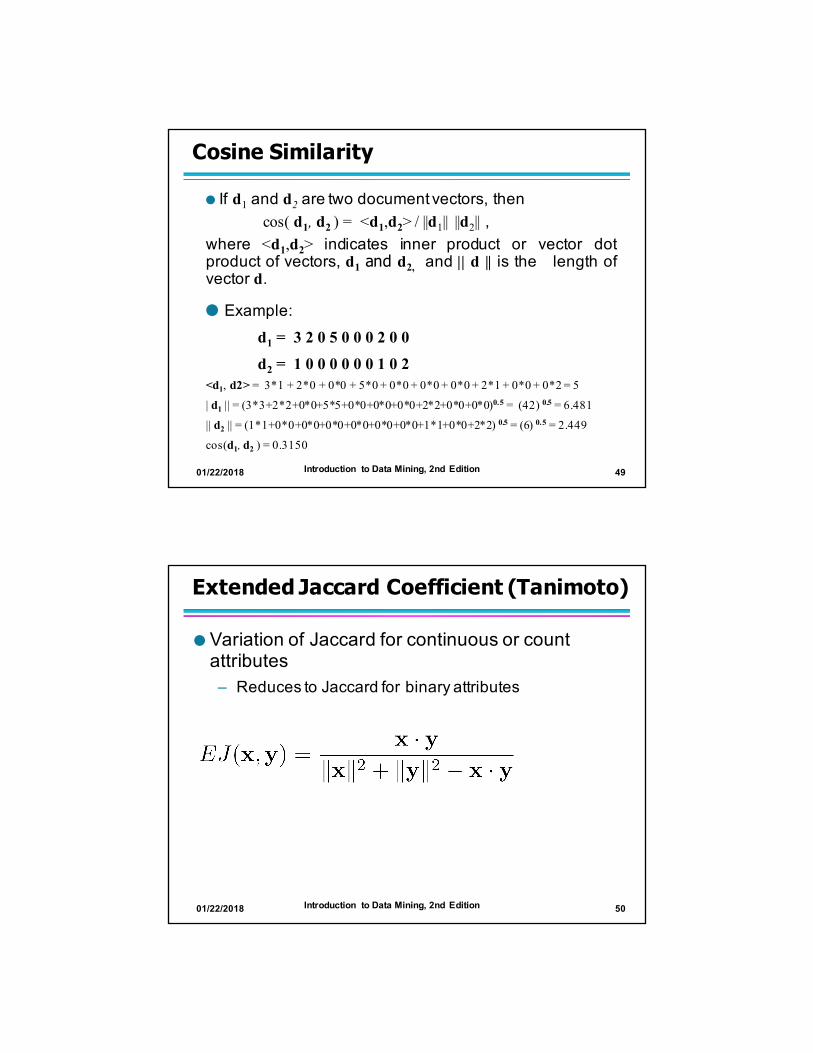
Euclidean Density: Grid-based Approach

Simplest approach is to divide region into a number of rectangular cells of equal volume and define density as # of points the cell contains

Grid-based density. Counts for each cell.


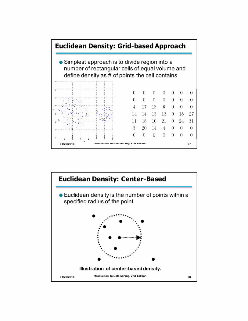
Euclidean Density: Center-Based

Euclidean density is the number of points within a specified radius of the point

Illustration of center-based density.


Data Preprocessing

Aggregation

Sampling

Dimensionality Reduction

Feature subset selection Feature creation

Discretization and Binarization

Attribute Transformation


Aggregation

Combining two or more attributes (or objects) into a single attribute (or object)

Purpose– Data reduction

u Reduce the number of attributes or objects– Change of scale

u Cities aggregated into regions, states, countries, etc.u Days aggregated into weeks, months, or years

– More “stable” datau Aggregated data tends to have less variability


Example: Precipitation in Australia

This example is based on precipitation in Australia from the period 1982 to 1993. The next slide shows – A histogram for the standard deviation of average monthly precipitation for 3,030 0.5 by 0.5 grid cells in Australia, and

– A histogram for the standard deviation of the average yearly precipitation for the same locations.

The average yearly precipitation has less variability than the average monthly precipitation.

All precipitation measurements (and their standard deviations) are in centimeters.


Example: Precipitation in Australia …

Standard Deviation of Average Monthly Precipitation

Standard Deviation of Average Yearly Precipitation

Variation of Precipitation in Australia


Sampling Sampling is the main technique employed for datareduction.– It is often used for both the preliminary investigation ofthe data and the final data analysis.

Statisticians often sample because obtaining theentire set of data of interest is too expensive ortime consuming.

Sampling is typically used in data mining becauseprocessing the entire set of data of interest is tooexpensive or time consuming.


Sampling …

The key principle for effective sampling is the following:

– Using a sample will work almost as well as using the entire data set, if the sample is representative

– A sample is representative if it has approximately the same properties (of interest) as the original set of data


Sample Size

8000 points 2000 Points 500 Points


Types of Sampling Simple Random Sampling– There is an equal probability of selecting any particular item

– Sampling without replacementu As each item is selected, it is removed from the population

– Sampling with replacementu Objects are not removed from the population as they are selected for the sample.

u In sampling with replacement, the same object can be picked up more than once

Stratified sampling– Split the data into several partitions;; then draw random samples from each partition


Sample Size

What sample size is necessary to get at least oneobject from each of 10 equal-sized groups.


Curse of Dimensionality

When dimensionality increases, data becomes increasingly sparse in the space that it occupies

Definitions of density and distance between points, which are critical for clustering and outlier detection, become less meaningful •Randomly generate 500 points

•Compute difference between max and min distance between any pair of points


Dimensionality Reduction

Purpose:– Avoid curse of dimensionality– Reduce amount of time and memory required by data mining algorithms

– Allow data to be more easily visualized– May help to eliminate irrelevant features or reduce noise

Techniques– Principal Components Analysis (PCA)– Singular Value Decomposition– Others: supervised and non-linear techniques


Dimensionality Reduction: PCA

Goal is to find a projection that captures the largest amount of variation in data

x2

x1

e


Dimensionality Reduction: PCA


Feature Subset Selection

Another way to reduce dimensionality of data Redundant features – Duplicate much or all of the information contained in one or more other attributes

– Example: purchase price of a product and the amount of sales tax paid

Irrelevant features– Contain no information that is useful for the data mining task at hand

– Example: students' ID is often irrelevant to the task of predicting students' GPA

Many techniques developed, especially for classification


Feature Creation

Create new attributes that can capture the important information in a data set much more efficiently than the original attributes

Three general methodologies:– Feature extraction

u Example: extracting edges from images– Feature construction

u Example: dividing mass by volume to get density– Mapping data to new space

u Example: Fourier and wavelet analysis


Mapping Data to a New Space

Two Sine Waves + Noise Frequency

Fourier and wavelet transform

Frequency


Discretization

Discretization is the process of converting a continuous attribute into an ordinal attribute– A potentially infinite number of values are mapped into a small number of categories

– Discretization is commonly used in classification– Many classification algorithms work best if both the independent and dependent variables have only a few values

– We give an illustration of the usefulness of discretization using the Iris data set


Iris Sample Data Set

Iris Plant data set.– Can be obtained from the UCI Machine Learning Repository http://www.ics.uci.edu/~mlearn/MLRepository.html

– From the statistician Douglas Fisher– Three flower types (classes):

u Setosau Versicolouru Virginica

– Four (non-class) attributesu Sepal width and lengthu Petal width and length Virginica. Robert H. Mohlenbrock. USDA

NRCS. 1995. Northeast wetland flora: Field office guide to plant species. Northeast National Technical Center, Chester, PA. Courtesy of USDA NRCS Wetland Science Institute.

Discretization: Iris Example

Petal width low or petal length low implies Setosa.Petal width medium or petal length medium implies Versicolour.Petal width high or petal length high implies Virginica.


Discretization: Iris Example …

How can we tell what the best discretization is?– Unsupervised discretization: find breaks in the data valuesuExample:Petal Length

– Supervised discretization:Use class labels to find breaks

0 2 4 6 80

10

20

30

40

50

Petal Length

Cou

nts


Discretization Without Using Class Labels

Data consists of four groups of points and two outliers. Data is one-dimensional, but a random y component is added to reduce overlap.



Equal interval width approach used to obtain 4 values.



Equal frequency approach used to obtain 4 values.



K-means approach to obtain 4 values.


Binarization

Binarization maps a continuous or categorical attribute into one or more binary variables

Typically used for association analysis

Often convert a continuous attribute to a categorical attribute and then convert a categorical attribute to a set of binary attributes– Association analysis needs asymmetric binary attributes

– Examples: eye color and height measured as low, medium, high


Attribute Transformation

An attribute transform is a function that maps the entire set of values of a given attribute to a new set of replacement values such that each old value can be identified with one of the new values– Simple functions: xk, log(x), ex, |x|– Normalization

u Refers to various techniques to adjust to differences among attributes in terms of frequency of occurrence, mean, variance, range

u Take out unwanted, common signal, e.g., seasonality

– In statistics, standardization refers to subtracting off the means and dividing by the standard deviation


Example: Sample Time Series of Plant Growth

Correlations between time series

Minneapolis

Minneapolis Atlanta Sao Paolo Minneapolis 1.0000 0.7591 -0.7581 Atlanta 0.7591 1.0000 -0.5739 Sao Paolo -0.7581 -0.5739 1.0000


Net Primary Production (NPP) is a measure of plant growth used by ecosystem scientists.


Seasonality Accounts for Much Correlation


Minneapolis

Normalized using monthly Z Score:Subtract off monthly mean and divide by monthly standard deviation

Minneapolis Atlanta Sao Paolo Minneapolis 1.0000 0.0492 0.0906 Atlanta 0.0492 1.0000 -0.0154 Sao Paolo 0.0906 -0.0154 1.0000


Documents

Lecture’Notesfor’Chapter’2 Introduction’to…kumar001/dmbook/slides/chap2_data… · 01/22/2018 Introduction/ toDataMining,2nd/Edition 1 Data$Mining:$Data Lecture’Notesfor’Chapter’2