Embed Size (px)
Citation preview

Lecturer’s desk
INTEGRATED LEARNING CENTER ILC 120
Screen
11 10
2 1
9 8 7 6 513 1215 14
17 1619 18
4 3
Row A
Row B
Row C
Row D
Row E
Row F
Row G
Row H
Row I
Row J
Row K
Row L
Com
pute
r Sto
rage
Cab
inet
Cabinet Cabinet Table
20
11 10
2 1
9 8 7 6 521 2023 22
25 2427 26
4 328
13 121416 15171819
11 10
2 1
9 8 7 6 521 2023 22
25 2426
4 3
13 121416 15171819
11 10
2 1
9 8 7 6 521 2023 22
25 2426
4 3
13 121416 15171819
11 10
2 1
9 8 7 6 521 2023 22
25 2427 26
4 328
13 121416 15171819
29 11 10
2 1
9 8 7 6 521 2023 22
25 2427 26
4 328
13 121416 15171819
11 10
2 1
9 8 7 6 521 2023 22
25 2427 26
4 3
13 121416 15171819
11 10
2 1
9 8 7 6 521 2023 22
25 2426
4 3
13 121416 15171819
11 10
2 1
9 8 7 6 521 2023 22
25 24 4 3
13 121416 15171819
11 10
2 1
9 8 7 6 521 2023 22
24 4 3
13 121416 15171819
11 10
2 1
9 8 7 6 521 2023 22
4 3
13 121416 15171819
11 10 9 8 7 6 5 4 3
13 121416 15171819
brokendesk

Introduction to Statistics for the Social Sciences
SBS200, COMM200, GEOG200, PA200, POL200, or SOC200Lecture Section 001, Fall, 2014
Room 120 Integrated Learning Center (ILC)10:00 - 10:50 Mondays, Wednesdays & Fridays.
http://www.youtube.com/watch?v=oSQJP40PcGI

Reminder
A note on doodling

Schedule of readings
Before next exam (November 21st)
Please read chapters 7 – 11 in Ha & Ha
Please read Chapters 2, 3, and 4 in PlousChapter 2: Cognitive Dissonance Chapter 3: Memory and Hindsight BiasChapter 4: Context Dependence

Homework due – Wednesday (November 12th)
On class website: Please print and complete homework worksheet #19
Using Excel for hypothesis testing with ANOVAs

Labs continue this week with Project 2
(with the exception of Tuesdays labs)


By the end of lecture today 11/10/14
Use this as your study guide
Hypothesis testing with Analysis of Variance (ANOVA)Constructing brief, complete summary statements

Study Type 2: t-test
Study Type 3: One-way Analysis of Variance (ANOVA)
Comparing more than two means
We are looking to compare two means

Single Independent Variable comparing more than two groups
Study Type 3: One-way ANOVA
Single Dependent Variable (numerical/continuous)
Independent Variable: Type of incentiveLevels of Independent Variable: None, Bike, Trip to Hawaii
Dependent Variable: Number of cookies soldLevels of Dependent Variable: 1, 2, 3 up to max sold
Between participant designCausal relationship: Incentive had an effect – it increased sales
Ian was interested in the effect of incentives for girl scouts on the number of cookies sold. He randomly assigned girl scouts into one of three groups. The three groups were given one of three incentives and looked to see whosold more cookies. The 3 incentives were 1) Trip to Hawaii, 2) New Bikeor 3) Nothing. This is an example of a true experiment
Used to test the effect of the IV on the DV
How could wemake this a
quasi-experiment?

Single Independent Variable comparing more than two groups
Study Type 3: One-way ANOVA
Single Dependent Variable (numerical/continuous)
Ian was interested in the effect of incentives for girl scouts on the number of cookies sold. He randomly assigned girl scouts into one of three groups. The three groups were given one of three incentives and looked to see whosold more cookies. The 3 incentives were 1) Trip to Hawaii, 2) New Bikeor 3) Nothing. This is an example of a true experiment
Used to test the effect of the IV on the DV
None New Bike
Sale
s per
Gir
l sc
out
TripHawaii
None New Bike
TripHawaii
Dependent variable is
always quantitative
In an ANOVA, independent variable is qualitative
(& more than two groups)
Sale
s per
Gir
l sc
out

Be careful you are not designing a Chi Square
One-way ANOVA versus Chi Square
None New Bike
Sale
s per
Gir
l sc
out
TripHawaii
This is an ANOVA
None New Bike
Tota
l N
um
ber
of
Box
es
Sold
TripHawaii
This is aChi Square
If this is just frequency you may have a
problem
These are
means
These are
means
These are
means
These are just frequencies
These are just frequencies
These are just frequencies

One-way ANOVA
One-way ANOVAs test only one independent variable- although there may be many levels
“Factor” = one independent variable “Level” = levels of the independent variable
• treatment• condition• groups
“Main Effect” of independent variable = difference between levels • Note: doesn’t tell you which specific levels (means) differ
from each other
A multi-factor experiment would be a multi-independent variables experiment
Number of cookies sold
Incentives
None Bike Hawaii trip

Comparing ANOVAs with t-tests
Similarities still include:
Using distributions to make decisions about common and rare events
Using distributions to make inferences about whether to reject the null hypothesis or not
The same 5 steps for testing an hypothesis
The three primary differences between t-tests and ANOVAS are:1. ANOVAs can test more than two means2. We are comparing sample means indirectly by
comparing sample variances3. We now will have two types of degrees of freedom t(16) = 3.0; p < 0.05 F(2, 15) = 3.0; p < 0.05
Tells us generally about number of
participants / observations
Tells us generally about number of
participants / observations
Tells us generally about number of
groups / levels of IV

A girlscout troop leader wondered whether providing an incentive to whomever sold the most girlscout cookies would
have an effect on the number cookies sold. She provided a big incentive to one troop (trip to Hawaii), a lesser
incentive to a second troop (bicycle), and no incentive to a third group, and then looked to see who sold more cookies.
Troop 1(Hawaii)
65946
Troop 2(bicycle)
68542
Note: 5 girls in each troop
Troop 3(nada)
0401 0
x = 6 x = 5
x = 1
What if we want to compare 3 means?One independent variable with 3 means

A girl scout troop leader wondered whether providing an incentive to whomever sold the most girl scout cookies would
have an effect on the number cookies sold. She provided a big incentive to one troop (trip to Hawaii), a lesser
incentive to a second troop (bicycle), and no incentive to a third group, and then looked to see who sold more cookies.
n = 5 x = 10
n = 5 x = 12
n = 5 x = 14
Troop 1(nada)
108
127
13
Troop 2(bicycle)
1214101113
Troop 3(Hawaii)
149
191315
What is Independent
Variable?
How many groups?
What is Dependent Variable?
How many levels of the Independent
Variable?

Main effect of incentive: Will offering an incentive result in more girl scout cookies being sold?
If we have a “effect” of incentive then the means are significantly different from each other• we reject the null• we have a significant F• p < 0.05
We don’t know which means are different from which …. just that they are not all the same
To get an effect we want:• Large “F”
- big effect and small variability• Small “p”
- less than 0.05 (whatever our alpha is)

Hypothesis testing:
Step 1: Identify the research problem
Describe the null and alternative hypotheses
Is there a significant difference in the number of cookie boxes sold between the girlscout troops that were
given the different levels of incentive?

Hypothesis testing:
Decision rule
= .05
Critical F (2,12) = 3.98
Degrees of freedom (between) = number of groups - 1
Degrees of freedom (within) = # of scores - # of groups
= 3 - 1 = 2
= (15-3) = 12*
*or = (5-1) + (5-1) + (5-1) = 12.

α= .05
Critical F(2,12)
= 3.89
F (2,12)AppendixB.4 (pg.518)

ANOVA table
?
df MS F
? ?
?
Source
Between
WithinTotal
??
SS
?
?
?
“SS” = “Sum of Squares”- will be given for exams
- you can think of this as the numerator in a standard
deviation formula

?
?
?
ANOVA table
128
df MS F
# groups - 1
# scores - number of groups
# scores - 1
2
12
14
Source
Between
WithinTotal
88
40
SS
? ?
????
“SS” = “Sum of Squares”- will be given for exams
3-1=2
15-3=12
15- 1=14

ANOVA table
ANOVA table
128
df MS F
2
12
14
Source
Between
WithinTotal
88
40
SS
MSbetween
MSwithin
SSwithin
dfwithin
20
7.33
SSbetween
dfbetween
8812
=7.33
40 2
=20
207.33
=2.73 2.73
402
8812
? ?
?

Make decision whether or not to reject null hypothesis
2.73 is not farther out on the curve than 3.89 so, we do not reject the null hypothesis
Observed F = 2.73Critical F(2,12) = 3.89
Conclusion: There appears to be no effect of type of incentive on number of girl scout cookies sold
F(2,12) = 2.73; n.s.
The average number of cookies sold for three different incentives were compared. The mean number of cookie boxes sold for the“Hawaii” incentive was 14 , the mean number of cookies boxes sold for the “Bicycle” incentive was 12, and the mean number of cookies sold for the “No” incentive was 10. An ANOVA was conducted and there appears to be no significant difference in the number of cookies sold as a result of the different levels of incentive F(2, 12) = 2.73; n.s.

Let’s do same problemUsing MS Excel
A girlscout troop leader wondered whether providing an incentive to whomever sold the most girlscout cookies would
have an effect on the number cookies sold. She provided a big incentive to one troop (trip to Hawaii), a lesser
incentive to a second troop (bicycle), and no incentive to a third group, and then looked to see who sold more cookies.
Troop 1(Nada)
108
127
13
Troop 2(bicycle)
1214101113
Troop 3(Hawaii)
149
191315
n = 5 x = 10
n = 5 x = 12
n = 5 x = 14

Let’s do same problemUsing MS Excel

Let’s do same problemUsing MS Excel

Let’s do oneReplication of study
(new data)

Let’s do same problemUsing MS Excel

Let’s do same problemUsing MS Excel

SSwithin
dfwithin
SSbetween
dfbetween
8812
=7.33
40 2
=20
207.33
=2.73
402
8812
MSbetween
MSwithin
# groups - 1
# scores - number of groups
# scores - 1
3-1=2
15-3=12
15- 1=14
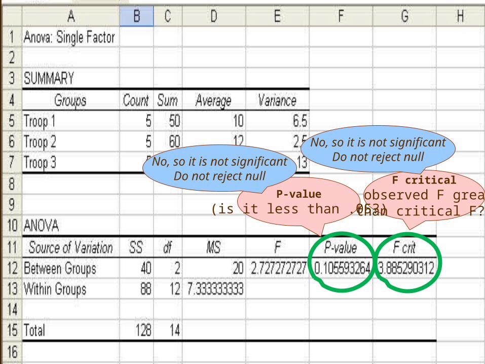
F critical
(is observed F greater than critical F?)
P-value
(is it less than .05?)
No, so it is not significantDo not reject null
No, so it is not significantDo not reject null
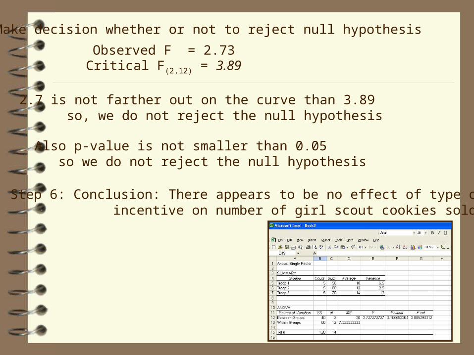
Make decision whether or not to reject null hypothesis
2.7 is not farther out on the curve than 3.89 so, we do not reject the null hypothesis
Observed F = 2.73Critical F(2,12) = 3.89
Also p-value is not smaller than 0.05 so we do not reject the null hypothesis
Step 6: Conclusion: There appears to be no effect of type of incentive on number of girl scout cookies sold

Make decision whether or not to reject null hypothesis
2.7 is not farther out on the curve than 3.89 so, we do not reject the null hypothesis
Observed F = 2.72727272Critical F(2,12) = 3.88529
Conclusion: There appears to be no effect of type of incentive on number of girl scout cookies sold
F(2,12) = 2.73; n.s.
The average number of cookies sold for three different incentives were compared. The mean number of cookie boxes sold for the“Hawaii” incentive was 14 , the mean number of cookies boxes sold for the “Bicycle” incentive was 12, and the mean number of cookies sold for the “No” incentive was 10. An ANOVA was conducted and there appears to be no significant difference in the number of cookies sold as a result of the different levels of incentive F(2, 12) = 2.73; n.s.

One way analysis of varianceVariance is divided
Total variability
Withingroup
variability(error variance)
Betweengroup
variability(only one factor)
Remember, 1 factor = 1 independent variable(this will be our numerator – like difference between
means)
Remember, error variance = random error
(this will be our denominator
– like within group variability
Remember, one-way = one IV

Five steps to hypothesis testing
Step 1: Identify the research problem (hypothesis)
Describe the null and alternative hypotheses
Step 2: Decision rule
• Alpha level? (α = .05 or .01)?
Step 3: Calculations
Step 4: Make decision whether or not to reject null hypothesisIf observed t (or F) is bigger then critical t (or F) then reject null
Step 5: Conclusion - tie findings back in to research problem
• Critical statistic (e.g. z or t or F or r) value?
MSWithin
MSBetweenF =
Still, difference between means
Still, variabilityof curve(s)

.Difference
between meansDifference
between meansDifference
between means
Variabilityof curve(s)Variabilityof curve(s)Variabilityof curve(s)
“Between Groups”Variability
“Within Groups”Variability

Sum of squares (SS): The sum of squared deviations of some set of scores about their mean
Mean squares (MS): The sum of squares divided by its degrees of freedom
Note: MStotal = MSwithin + MSbetween
Mean square within groups:sum of squares within groups divided by its degrees of freedom
Mean square between groups:sum of squares between groups divided by its degrees of freedom
Mean square total: sum of squares totaldivided by its degrees of freedom
MSWithin
MSBetweenF =

ANOVA
Variability within groups
Variability between groupsF =
Variability Between Groups
Variability Within Groups Variability Within Groups
“Between” variability bigger than “within” variability so
should get a big (significant) F
Variability Between Groups
Variability Within Groups Variability Within Groups
“Between” variability getting smaller “within” variability
staying same so, should get a smaller F
Variability Between Groups “Between” variability getting very small “within” variability staying same so, should get a
very small F
Variability Within Groups Variability Within Groups

ANOVAVariability within groups
Variability between groupsF =
“Between” variability bigger than “within” variability so
should get a big (significant) F
“Between” variability getting smaller “within” variability
staying same so, should get a smaller F
“Between” variability getting very small “within” variability staying same so, should get a
very small F (equal to 1)
Variability Within Groups
Variability Between Groups
Variability Within Groups
Variability Within Groups
Variability Between Groups

.
Effect size is considered relativeto variability of distributions
Treatment
Effect
Treatment
Effect
x
xVariability
within groups
Variability between groups
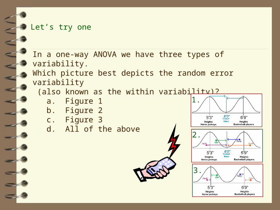
Let’s try one
In a one-way ANOVA we have three types of variability. Which picture best depicts the random error variability (also known as the within variability)? a. Figure 1 b. Figure 2 c. Figure 3 d. All of the above
1.
2.
3.

Let’s try one
Which figure would depict the largest F ratio a. Figure 1 b. Figure 2 c. Figure 3 d. All of the above
Variability within groups
Variability between groupsF =
1.
2.
3.
“F ratio” is referring to "observed F”

Let’s try one
Winnie found an observed z of .74, what should she conclude?
(Hint: notice that .74 is less than 1) a. Reject the null hypothesis b. Do not reject the null hypothesis c. Not enough info is given
small observed z score
xsmall observed z score
x
If your observed z is within one standard deviation of the mean,
you will never reject the null

Let’s try one
Winnie found an observed t of .04, what should she conclude?
(Hint: notice that .04 is less than 1) a. Reject the null hypothesis b. Do not reject the null hypothesis c. Not enough info is given
small observed t score
x

Let’s try one
Winnie found an observed F ratio of .9, what should she conclude? a. Reject the null hypothesis b. Do not reject the null hypothesis c. Not enough info is given
1.
2.
3.