Lectures 3 to 9

THE ANALYSIS OF PSYCHOLOGICAL DATA

Your lecturer and course convener

• Colin Gray

• Room S16 William Guild Building

• E-mail address: c.gray@abdn.ac.uk

• Telephone: (27) 2233

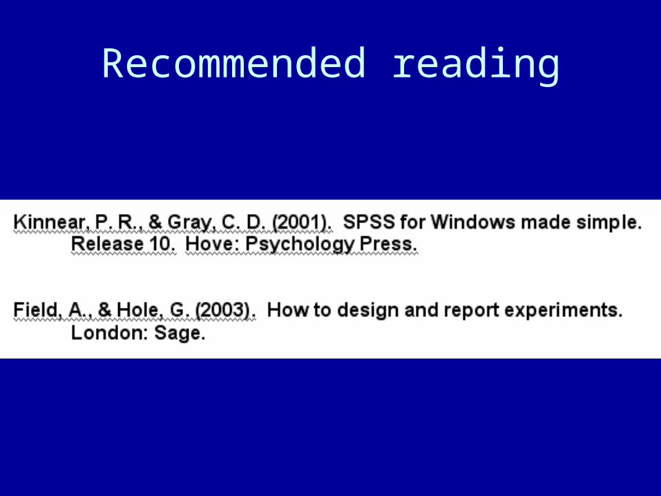
Recommended reading

The examination

• Multiple-choice format.

• Examples during the lectures.

• Last year’s papers are in the library.

• All course lecturers should provide you with examples.

SPSS update

• SPSS frequently brings out new versions.• You have learned about SPSS 10.• The university now runs SPSS 12.• Previously, they maintained the previous

version as well as the current version, but not this year.

• I shall draw your attention to the differences between SPSS 10 and SPSS 12 in these lectures.

Preliminary reading

• Chapter 1 in Kinnear & Gray (2001). – Research terminology.– Advice on choosing a statistical test.

• Chapter 1 in Field & Hole (2003) ranges more widely, with consideration of the theoretical and philosophical foundations of psychological research.

Lecture 1

REVISION

Three strategies in psychological research

1. Experimental

2. Correlational

3. Observational

1. Experimental research

• In experimental research, the experimenter MANIPULATES one variable to demonstrate that it has a CAUSAL EFFECT upon another, which is MEASURED or recorded during the course of the experiment.

• Such manipulation is the hallmark of a true experiment.

The independent and dependent variables

• The manipulated variable is known as the INDEPENDENT VARIABLE (IV).

• The measured variable is known as the DEPENDENT VARIABLE (DV).

• The experimental results should show whether the IV has a causal effect upon the DV.

A research question

• Does the ingestion of a dose of caffeine improve performance on a skilled task?

• We shall design an experiment to answer this question.

Performance on a skilled task

• The participants play a computer game that simulates shooting at a target.

• Each participant ‘shoots’ twenty times at a target and receives one point for each ‘hit’.

• The PERFORMANCE MEASURE is the total number of hits by each participant, so each participant receives a score from 0 to 20.

• Number of Hits is the DEPENDENT VARIABLE in this experiment.

The independent variable

• The independent variable is Drug Treatment, one condition of which is the ingestion of a dose of caffeine.

Placebo effects

• The mere fact of receiving something to drink may affect the dependent variable. This is known as a PLACEBO EFFECT.

• So what is needed is a comparison treatment condition in which the participant receives a preparation similar to the medium in which the active agent is presented.

• The control group must also be given a caffeine-free drink.

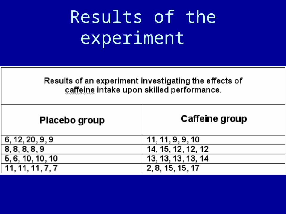
Results of the experiment

Has the experiment worked?

• It’s difficult to make sense of a collection of numbers or RAW DATA like this.

• There certainly seem to be more high scores in the Caffeine section.

• But the highest score (20) is in the Placebo group, not the Caffeine group.

• And the lowest score (2) is in the Caffeine group, not the Placebo group.

Summarising the data

• We can do this in two ways:

1. We can make a PICTURE OF THE DATA.

2. We can use NUMERICAL measures known as STATISTICS that bring out certain features of the data as a

whole.

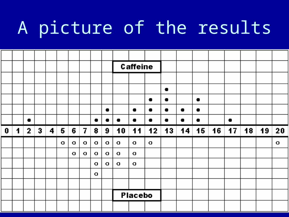
A picture of the results

Distributions

• The DISTRIBUTION of a variable is a profile of the relative frequencies with which its values occur across the entire range of variation.

• The picture shows the distributions of Performance for the participants in the Caffeine and Placebo groups.

Interpreting the picture

• A clear pattern emerges: the scores of the Caffeine group cluster around a higher value than do those of the Placebo group.

• Typically, the Caffeine group score at a higher LEVEL than do the Placebo group.

Interpreting the data…

• The picture suggests that the level for the Caffeine group (ie the region in which scores are commonest) is around 12 - 13.

• The level for the Placebo group is around 8 - 9.

Measures of level: on the average

• In Statistics, an AVERAGE is a measure of level or CENTRAL TENDENCY. An average is a value TYPICAL of the data as a whole.

• There are several different averages. One is the MEAN. Another is the MEDIAN.

• The MEAN is the sum of all the scores, divided by the number of scores.

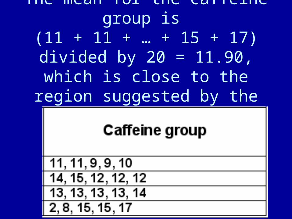
The mean for the Caffeine group is (11 + 11 + … + 15 + 17) divided by

20 = 11.90, which is close to the region suggested by the picture.

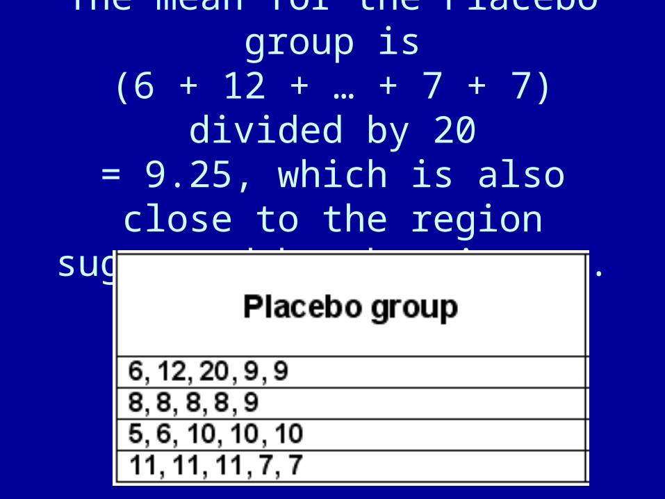
The mean for the Placebo group is(6 + 12 + … + 7 + 7) divided by 20= 9.25, which is also close to the region suggested by the picture.

A warning

• If the value of the mean doesn’t appear to be consistent with a picture of the data set, the mean may be the wrong kind of average to use.

• The median, for instance, might be a better choice.

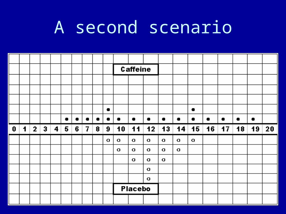
A second scenario

Interpretation of Scenario 2

• The mean Performance score is 12 for both groups.

• But in the Caffeine distribution, the scores are more widely SPREAD out or DISPERSED than those of the Placebo group.

• Perhaps caffeine helps some but impedes others?

Dispersion or spread

• The DISPERSION of a distribution is the extent to which scores are spread out around or DEVIATE from the central mean.

• There are several ways of measuring dispersion.

The simple range

• The SIMPLE RANGE is the highest score minus the lowest score.

• So, for the Placebo group, the simple range is (15 – 9) = 6 score units.

• For the Caffeine group, the simple range is (19 – 5) = 14 score units.

• The Caffeine distribution shows two and a half times as much spread or dispersion of scores around the mean.

A problem with the simple range

• The simple range statistic only uses two scores out of the whole distribution.

• Should the scores be highly atypical of the distribution, the range may not reflect the typical spread of scores about the mean of the distribution.

• Nevertheless, the range can be a very useful statistic when you are exploring a data set.

The variance and the standard deviation (SD)

• The VARIANCE and the STANDARD DEVIATION (SD) are also measures of dispersion.

• Both statistics use the values of all the scores in the distribution.

• For details, see Appendix to this lecture.

Scenario 3

Ceiling effect

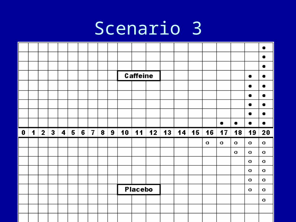
• The mean score for the Caffeine group is 19.35; the mean for the Placebo group is 19.00.

• That might suggest that caffeine has no effect. • But look at the SHAPES of the distributions of

Performance for the Caffeine and Placebo groups.

• The scores are bunched around the top of the scale.

• Any possible effect of caffeine intake has been masked by a CEILING EFFECT.

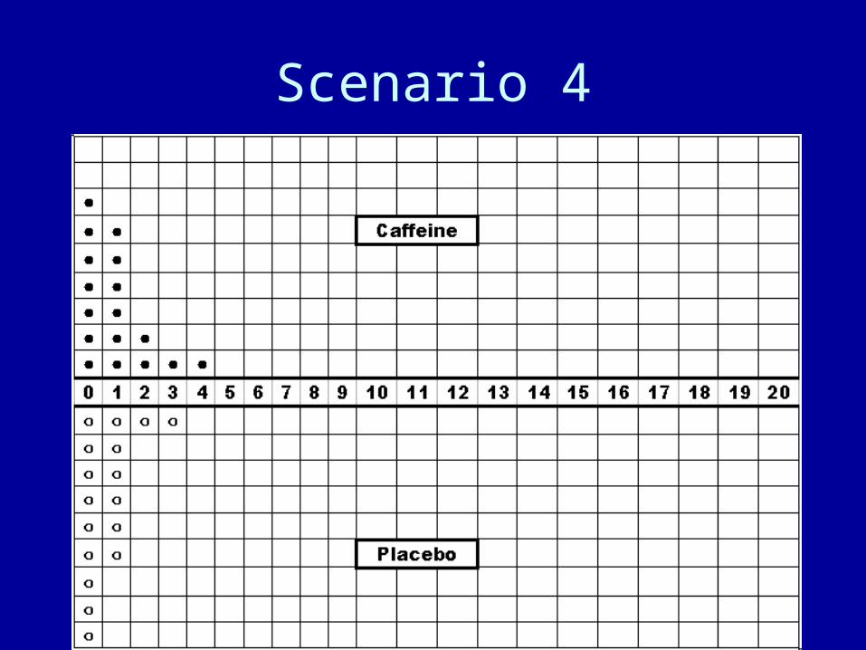
Scenario 4

Floor effect

• The mean score for the Caffeine group is .71; the mean for the Placebo group is .514.

• That might suggest that caffeine has no effect. • But look at the SHAPES of the distributions of

Performance for the Caffeine and Placebo groups.

• The scores are bunched around the bottom of the scale.

• Any possible effect of caffeine intake has been masked by a FLOOR EFFECT.

Skewness

• In both Scenarios 3 and 4, the distributions are twisted or SKEWED.

• When a distribution has a tail to the left, it is said to be NEGATIVELY SKEWED; when it has a tail to the right, it is POSITIVELY SKEWED.

• In Scenario 3, the distribution are negatively skewed; in Scenario 4 they are positively skewed.

Skewness and difficulty level

• A negatively skewed distribution can indicate that the task is too simple.

• This is known as a CEILING EFFECT.• A positively skewed distribution can

indicate that the task is too difficult. • This is known as a FLOOR EFFECT. • The Placebo distribution shows a floor

effect; the Caffeine distribution shows a ceiling effect.

A distribution has three important aspects

1. The typical value, CENTRAL TENDENCY or AVERAGE of the scores.

2. The degree to which the scores are DISPERSED or spread out around the average.

3. Its SHAPE.

Uses of statistics

1. We use statistics to DESCRIBE our data.

2. We use statistics to CONFIRM our data.

Our research question

• Does caffeine improve performance?

• We have found that the 20 people in the Placebo group had a mean accuracy of 9.25 and the 20 people in the Caffeine group had a mean of 11.90.

• That’s a mean difference of (11.90 – 9.25) = 2.65.

Generalising from a data set

• But the research question isn’t about the 40 people I have studied: it’s about whether caffeine improves the performance of ALL people.

• I have data on the performance of SOME people.

• Can I conclude that caffeine tends to improve the performance of ALL people?

Population

• I have SOME performance scores. • The population is the REFERENCE SET

of ALL scores that could, in principle, be obtained under the same conditions.

• I have a SAMPLE from that population. • I found a mean difference between the

Caffeine and Placebo of 2.65 hits. • But is there a substantial difference in the

population?

Sampling variability

• Sampling implies SAMPLING VARIABILITY.

• The smaller the samples we take, the more variability they show.

Statistics versus parameters

• STATISTICS are characteristics of SAMPLES; PARAMETERS are characteristics of POPULATIONS.

• Parameters have fixed values; but statistics vary because of sampling variability.

Statistics show variation

• If I test the shooting accuracy of more people, I shall find that the values of the mean and SD are different from the corresponding values in the first people I tested.

• When I ran my experiment, I found a mean difference of 2.65 points. If I were to repeat the experiment, I wouldn’t get exactly that difference on the second occasion.

Statistical inference

• We found that the mean of the Placebo group was 9.25 and the mean of the Caffeine group was 11.90. The difference is 2.65 points.

• I can use these values as ESTIMATES of the corresponding PARAMETERS (the population values).

• This is an example of STATISTICAL INFERENCE.

Statistical error

• Because of sampling variability, the means (and their difference) that I obtained are likely to differ from the corresponding parameters.

• My values, in this sense, are subject to ERROR. • Some error need not be a problem. But I want to

be confident that if the experiment were to be repeated we would still obtain a substantial difference between the Caffeine and Placebo means.

Statistical inference

1. Point estimation. The values of the statistics of your data are point estimates of the corresponding parameters.

2. Interval estimation. Around your values you can build intervals, called CONFIDENCE INTERVALS, within which you can be confident to a specified level that the parameters lie.

3. Hypothesis testing.

Probability

• A probability is a measure of likelihood ranging from 0 to 1.

• An event which is impossible has a probability of 0.

• An event which is certain has a probability of 1.

• An event which is neither certain nor impossible has a probability between 0 and 1.

2. Interval estimation

• The statistics from our data (the means, SDs and the difference between means) are point estimates.

• Around each we can build the 95% and 99% confidence intervals, that is ranges of values within which we can be 95% and 99% confident that the true parameter values lie.

Confidence interval for the difference between means

• I found a difference between the Placebo and Caffeine means of 2.65.

• I can construct an interval around that difference such that I can be, say, 95% confident that the true population difference lies within the interval.

3. Hypothesis testing

• In classical hypothesis testing, the NULL HYPOTHESIS states that there is NO DIFFERENCE. (So in our experiment, caffeine has no effect.)

• The ALTERNATIVE HYPOTHESIS states that there IS a difference. This is the equivalent of the scientific hypothesis that caffeine has an effect.

Hypothesis testing…

• In classical statistical inference, it is the NULL HYPOTHESIS, not the alternative hypothesis, that is tested directly. Should the null hypothesis fail the test, we conclude that we have evidence for the alternative hypothesis.

• We make the test of the null hypothesis with a TEST STATISTIC.

Hypothesis testing…

• The value of the test statistic (t, F, chi-square) is calculated from the data.

• If the value has a sufficiently LOW probability under the null hypothesis, the null hypothesis is rejected.

The t statistic

• The null hypothesis is that, in the population, there is no difference between the Caffeine and Placebo means.

• From the mean scores of the Caffeine and Placebo groups, the SDs and the numbers of observations in each group, we find the value of the t statistic.

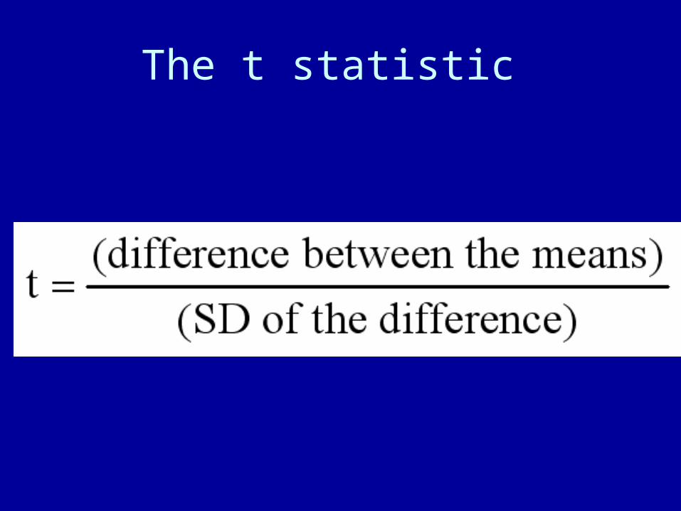
The t statistic

The t distribution

• Like any other statistic, the value of t shows variation from sample to sample.

• If the null hypothesis is correct, the mean of the t distribution is zero (no difference).

• If you have a large sample (say 50 in each group), then a value of t of at least plus or minus 2 is less likely than .05 under the null hypothesis.

Specifying a t distribution

• There is a whole family of t distributions.

• To decide upon the significance of your value of t, you must specify which t distribution you are referring to.

• To do that, you must specify the DEGREES OF FREEDOM (df).

• The df is calculated from the numbers of scores in the two groups.

The p-value

• The p-value of a test statistic is the probability, under the null hypothesis, of obtaining a value at least as unlikely under the null hypothesis as the value obtained.

Significance levels

• A test is said to show ‘significance’ if the p-value is less than a small probability (fixed by convention), known as a ‘significance level’.

• There are two conventional significance levels: .05 and .01.

A statistically significant result

• If the p-value is less than .05 but more than .01, the result of the test is ‘significant beyond the .05 level’.

• If the p-value is less than .01, the result is ‘significant beyond the .01 level’.

Remember!

• A small p-value (say p = .0001) is evidence AGAINST the null hypothesis.

• Often, therefore, a low p-value confirms the SCIENTIFIC HYPOTHESIS.

• A large p-value (say .7 or higher) would be BAD news because your scientific hypothesis receives no confirmation.

BUT …

• Sometimes you want to ACCEPT the null hypothesis.

• Suppose you construct two tests and hope to show they are of similar difficulty.

• You give the test to two samples of people and test the difference between the means.

• You want the p-value to be HIGH (say p = .8) so that there is no reason to question your claim of equal difficulty.

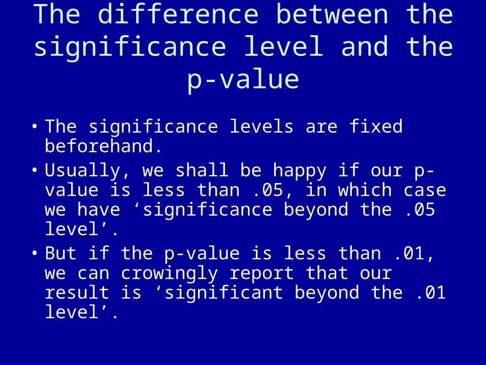
The difference between the significance level and the p-value

• The significance levels are fixed beforehand.

• Usually, we shall be happy if our p-value is less than .05, in which case we have ‘significance beyond the .05 level’.

• But if the p-value is less than .01, we can crowingly report that our result is ‘significant beyond the .01 level’.

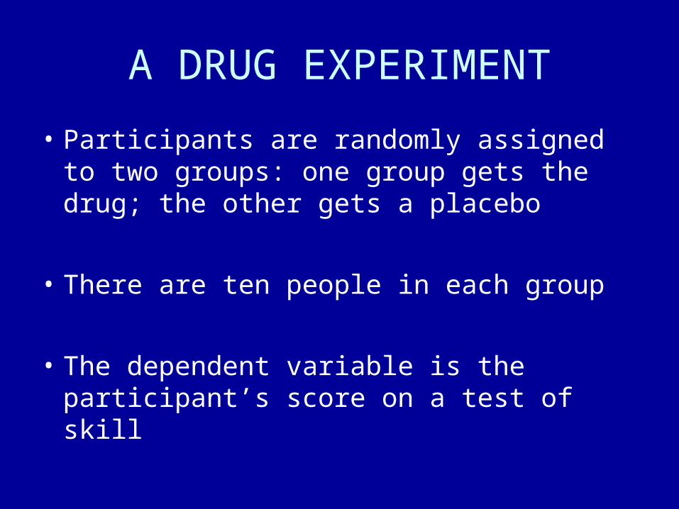
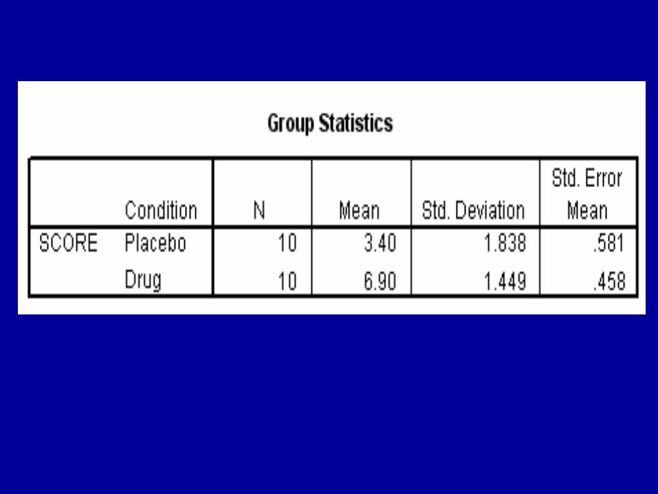
A DRUG EXPERIMENT

• Participants are randomly assigned to two groups: one group gets the drug; the other gets a placebo

• There are ten people in each group

• The dependent variable is the participant’s score on a test of skill

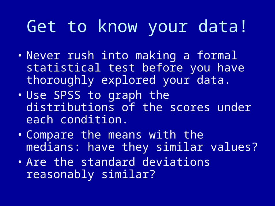
Get to know your data!

• Never rush into making a formal statistical test before you have thoroughly explored your data.

• Use SPSS to graph the distributions of the scores under each condition.

• Compare the means with the medians: have they similar values?

• Are the standard deviations reasonably similar?

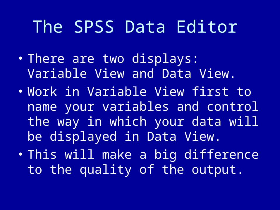
The SPSS Data Editor

• There are two displays: Variable View and Data View.

• Work in Variable View first to name your variables and control the way in which your data will be displayed in Data View.

• This will make a big difference to the quality of the output.

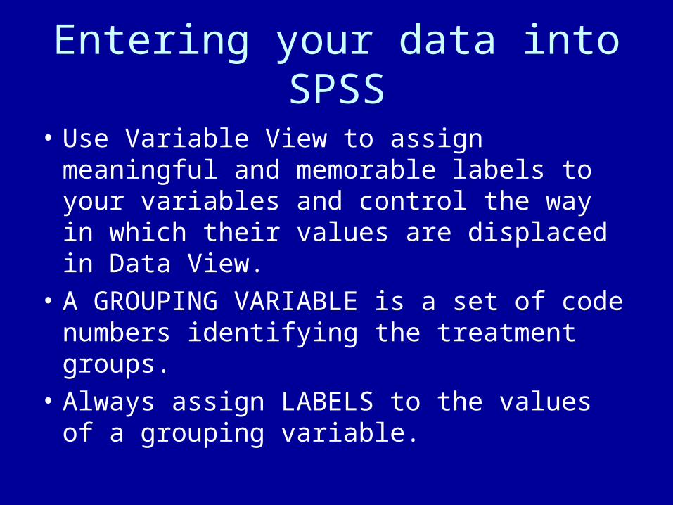
Entering your data into SPSS

• Use Variable View to assign meaningful and memorable labels to your variables and control the way in which their values are displaced in Data View.

• A GROUPING VARIABLE is a set of code numbers identifying the treatment groups.

• Always assign LABELS to the values of a grouping variable.

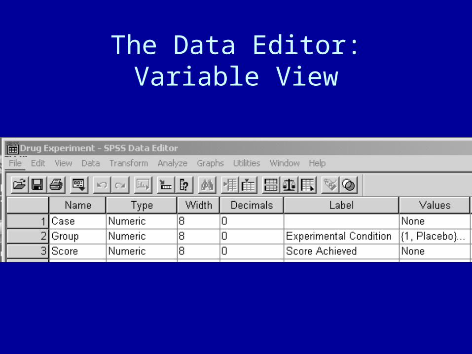
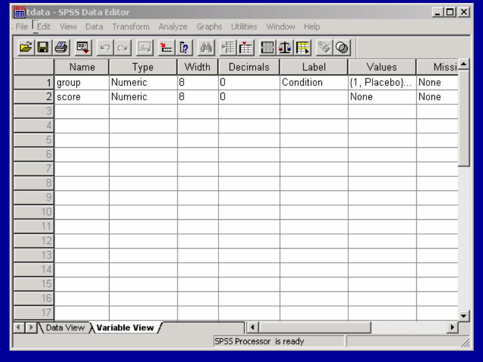
The Data Editor:Variable View

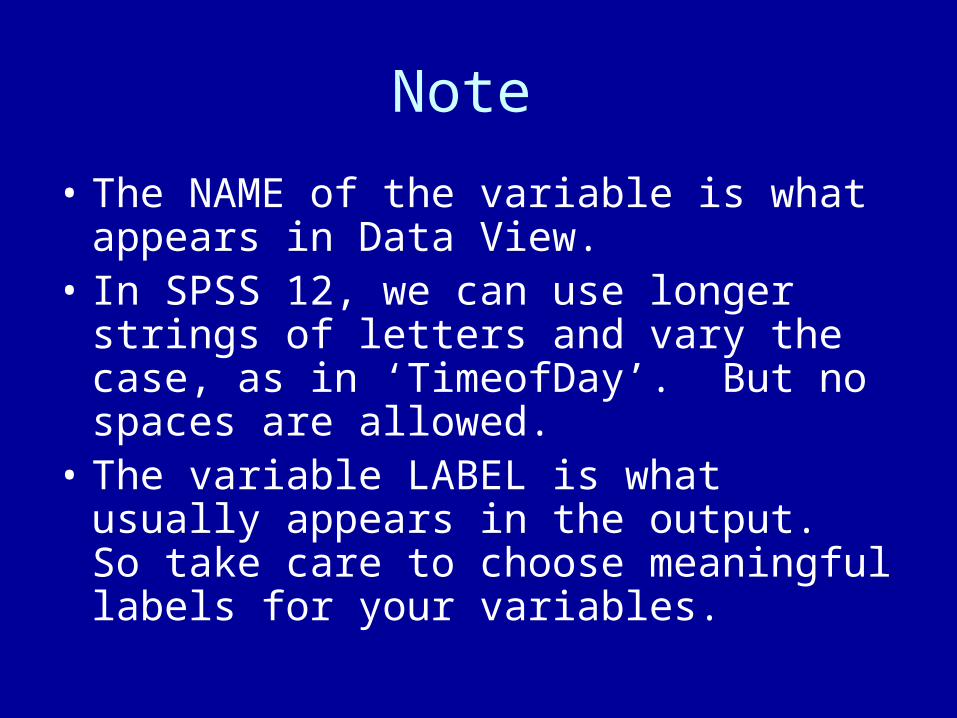
Note

• The NAME of the variable is what appears in Data View.

• In SPSS 12, we can use longer strings of letters and vary the case, as in ‘TimeofDay’. But no spaces are allowed.

• The variable LABEL is what usually appears in the output. So take care to choose meaningful labels for your variables.

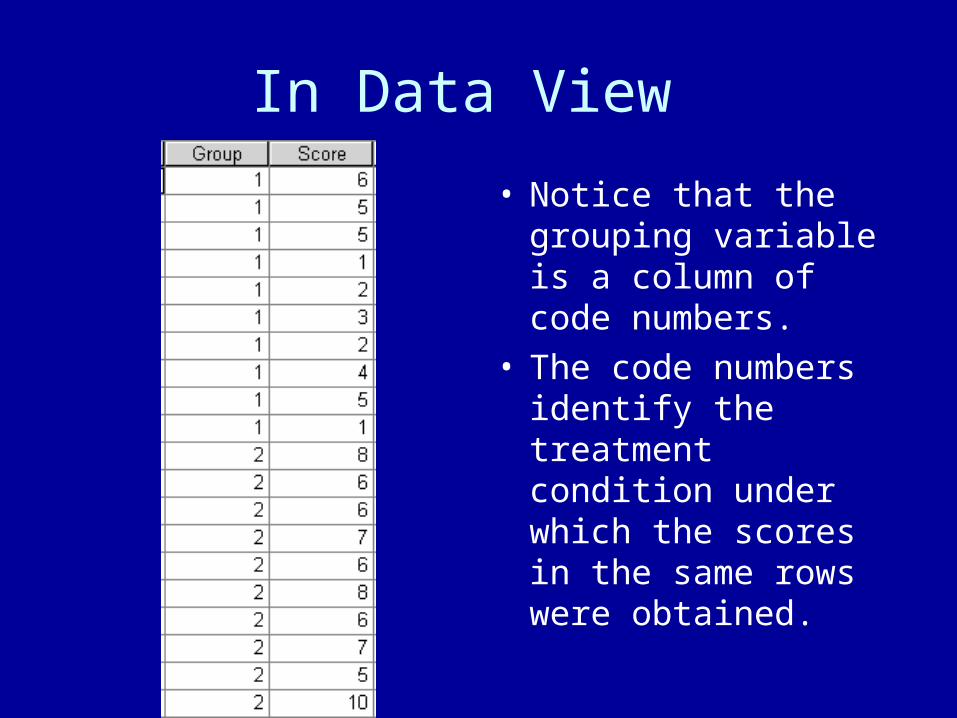
In Data View

• Notice that the grouping variable is a column of code numbers.

• The code numbers identify the treatment condition under which the scores in the same rows were obtained.

Data View

• When entering your data in Data View, it is often useful to have the value labels visible, rather than the code numbers.

• Display the value labels by choosing Value Labels from the View menu.

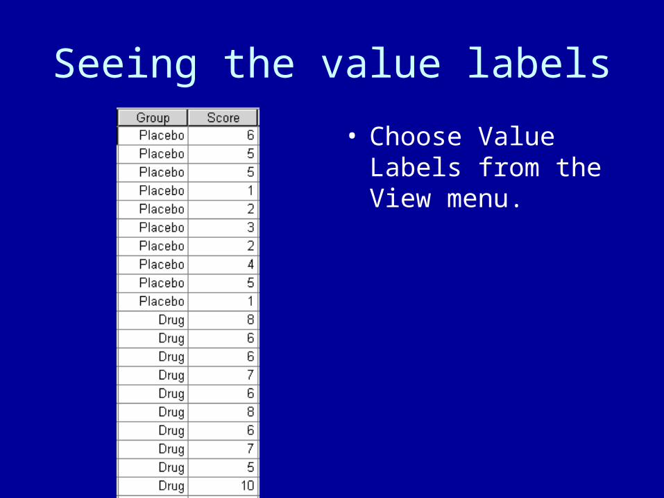
Seeing the value labels

• Choose Value Labels from the View menu.

Choosing the test

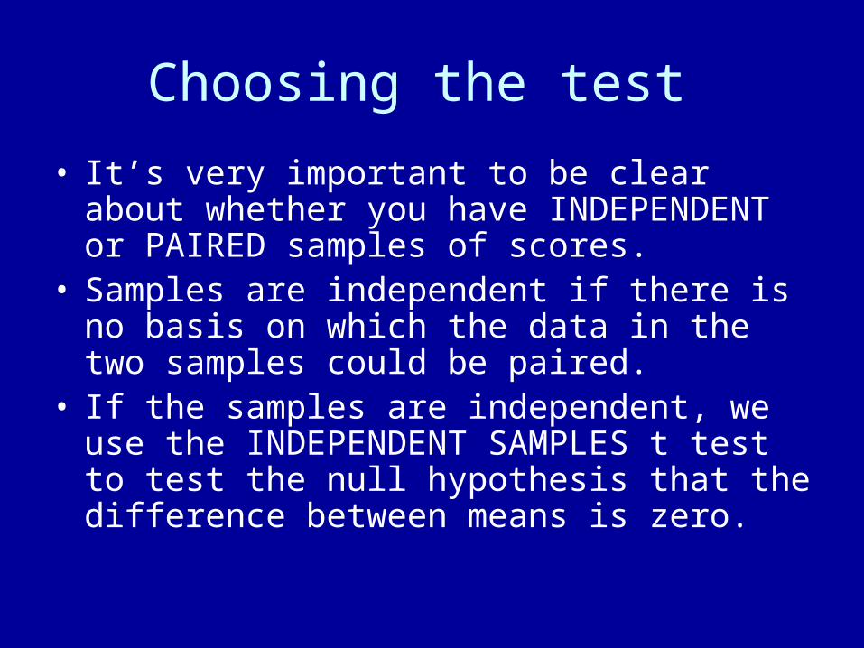
• It’s very important to be clear about whether you have INDEPENDENT or PAIRED samples of scores.

• Samples are independent if there is no basis on which the data in the two samples could be paired.

• If the samples are independent, we use the INDEPENDENT SAMPLES t test to test the null hypothesis that the difference between means is zero.

The independent samples t test

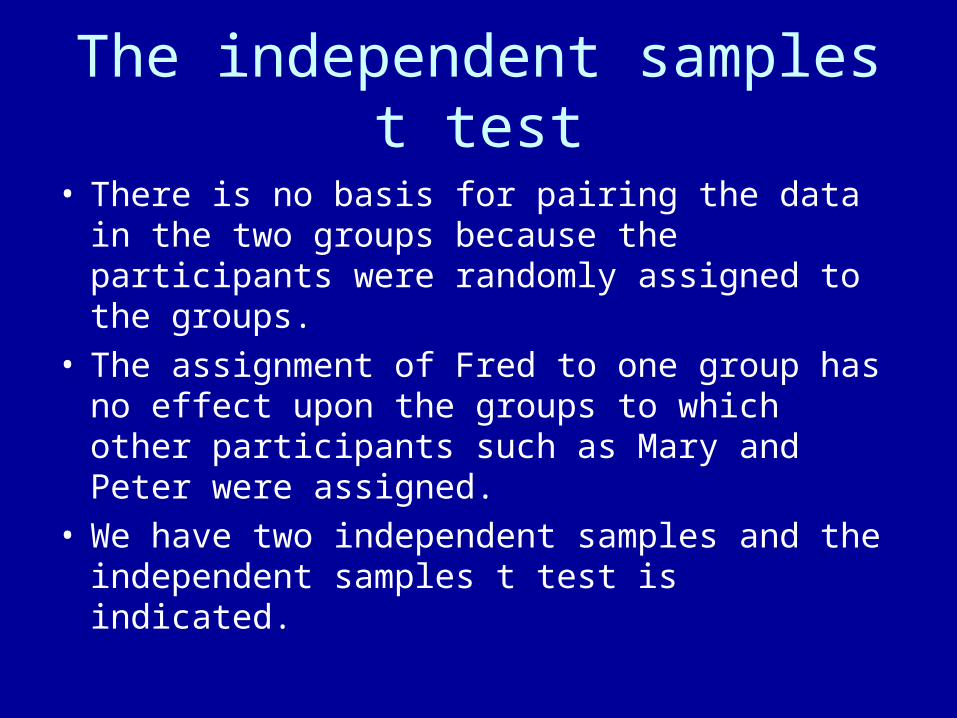
• There is no basis for pairing the data in the two groups because the participants were randomly assigned to the groups.

• The assignment of Fred to one group has no effect upon the groups to which other participants such as Mary and Peter were assigned.

• We have two independent samples and the independent samples t test is indicated.

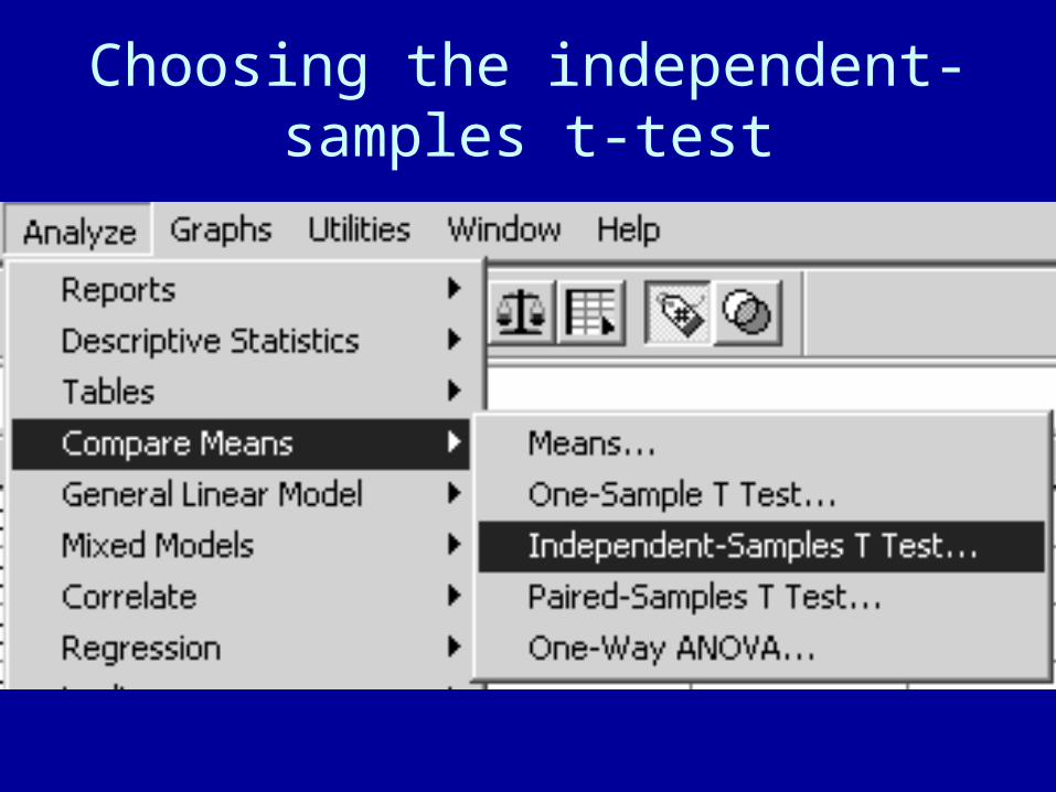
Choosing the independent-samples t-test

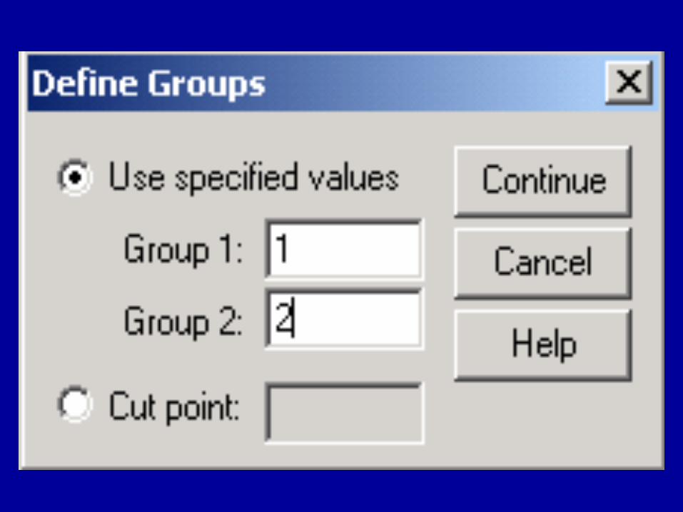
The t-test dialog box

• To get the Define Groups button to come alive, you must click on Grouping Variable.

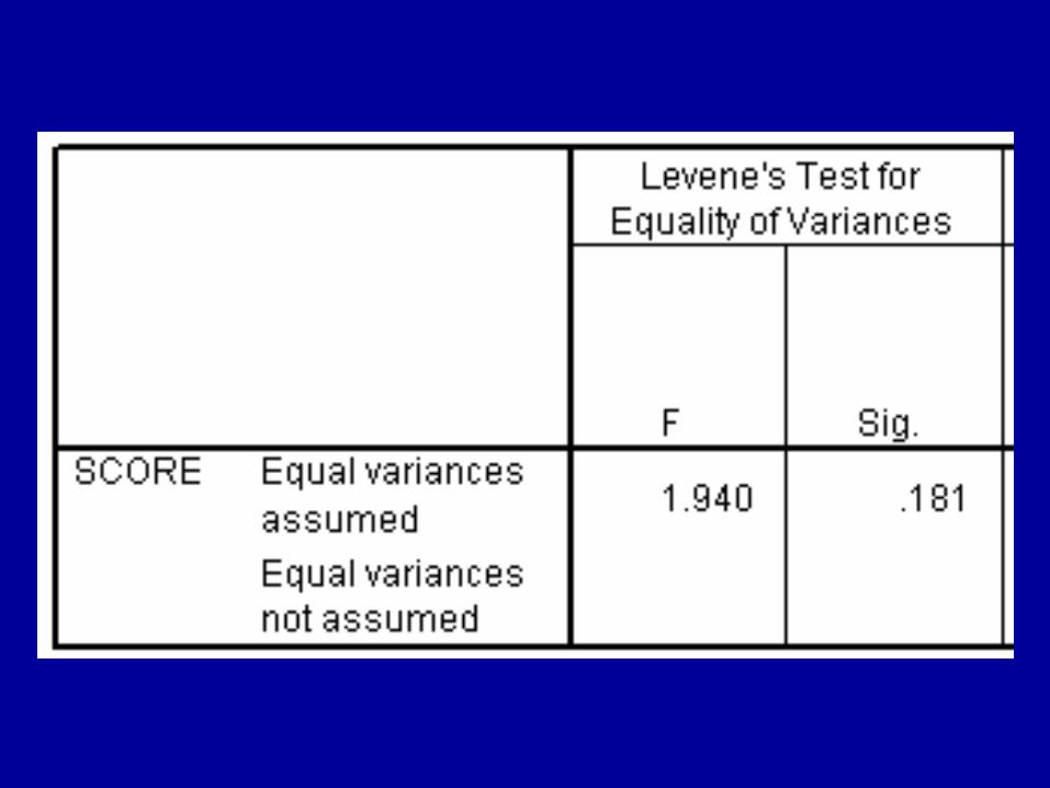
Levene’s test

• The model underlying the t-test assumes that the populations have equal variances.

• If Levene’s test gives a value of F with a high p-value, the assumption of equal variances is tenable.

• If the p-value from the Levene test is small, choose the report of the SEPARATE-VARIANCES T TEST, which is given in the second row of the same table.

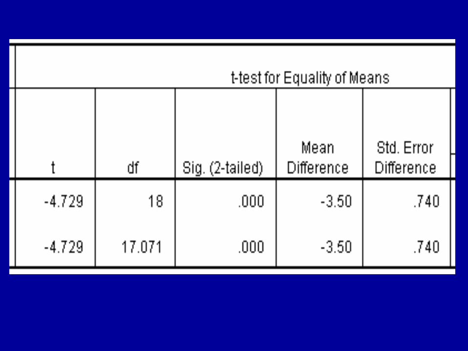
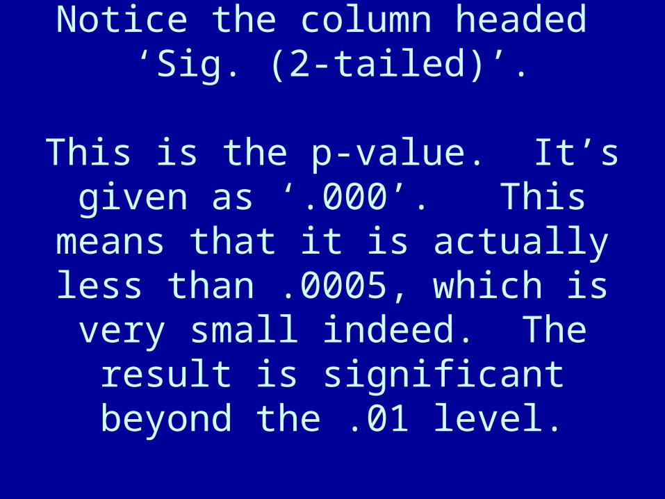
Notice the column headed ‘Sig. (2-tailed)’.

This is the p-value. It’s given as ‘.000’. This means that it is

actually less than .0005, which is very small indeed. The result is significant beyond the .01 level.

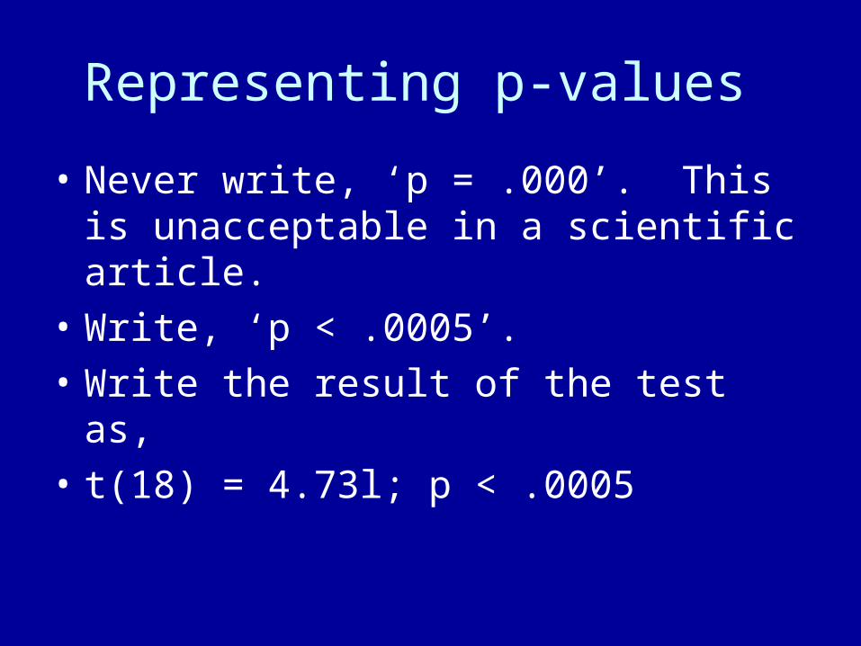
Representing p-values

• Never write, ‘p = .000’. This is unacceptable in a scientific article.

• Write, ‘p < .0005’.

• Write the result of the test as,

• t(18) = 4.73l; p < .0005

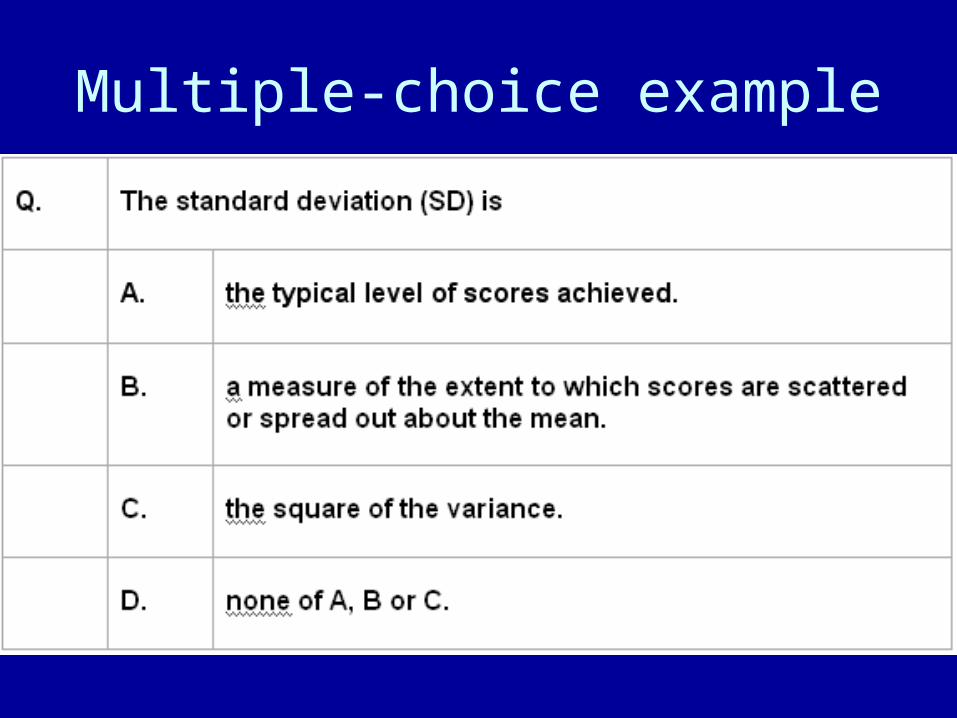
Multiple-choice example

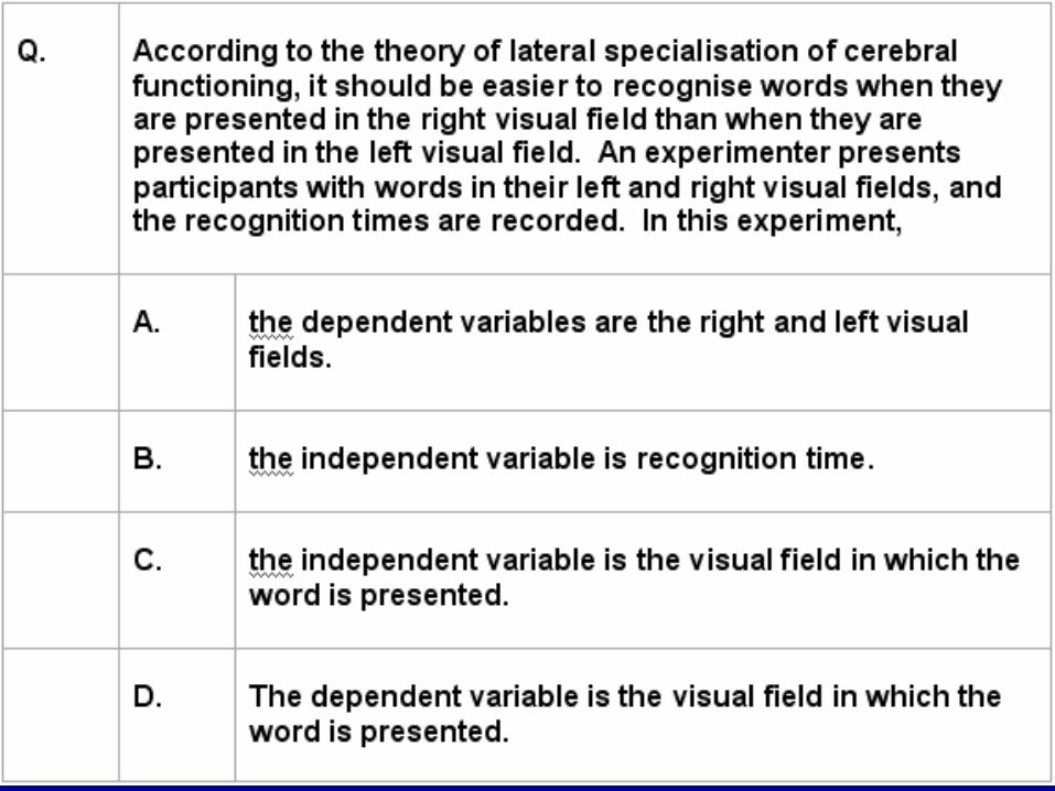
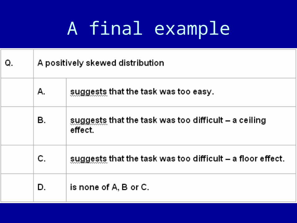
A final example

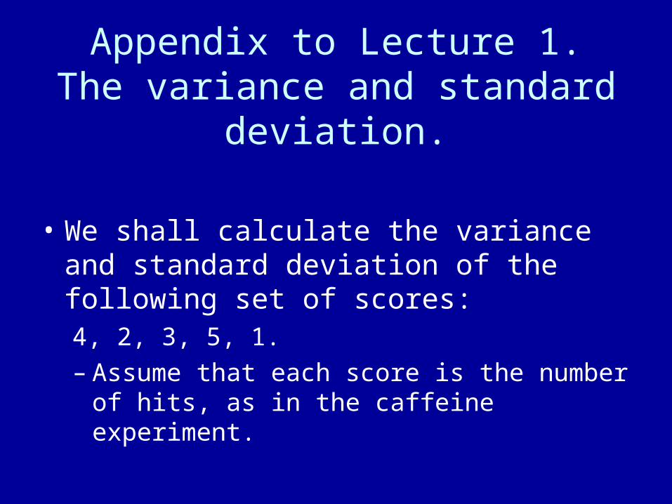
Appendix to Lecture 1.The variance and standard

deviation.

• We shall calculate the variance and standard deviation of the following set of scores: 4, 2, 3, 5, 1. – Assume that each score is the number of hits,

as in the caffeine experiment.

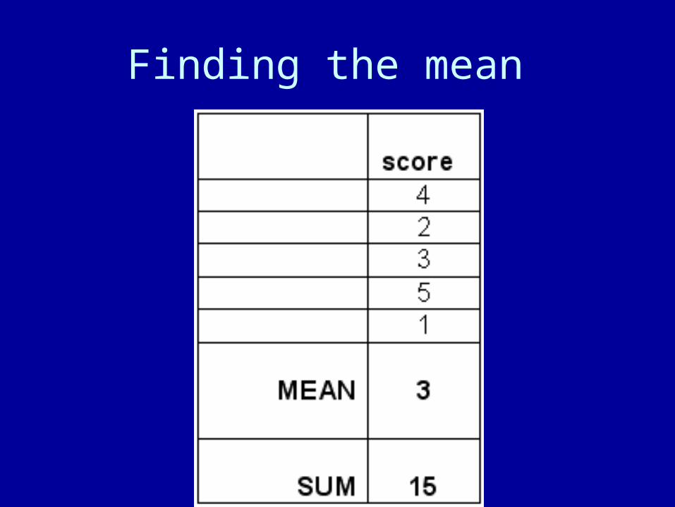
Finding the mean

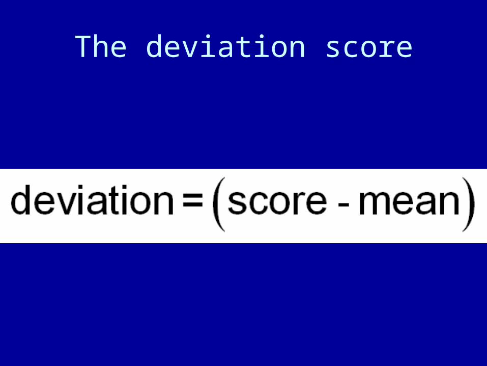
The deviation score

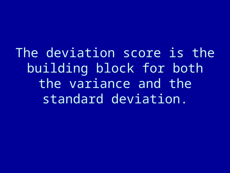
The deviation score is the building block for both the variance and the

standard deviation.

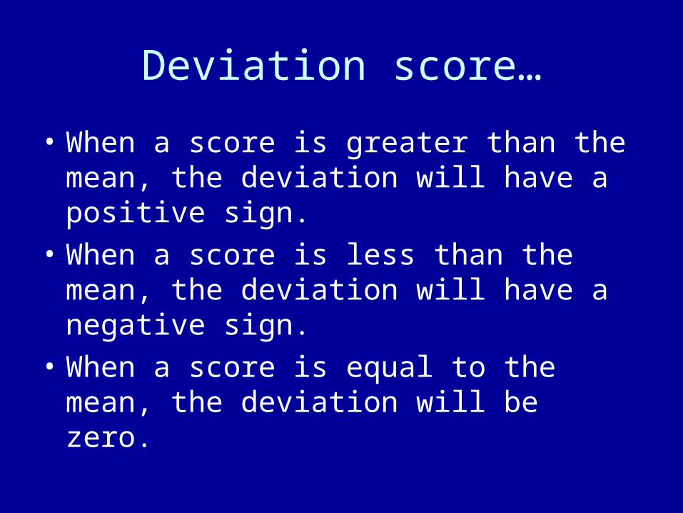
Deviation score…

• When a score is greater than the mean, the deviation will have a positive sign.

• When a score is less than the mean, the deviation will have a negative sign.

• When a score is equal to the mean, the deviation will be zero.

Could we use the mean deviation as our measure of dispersion?

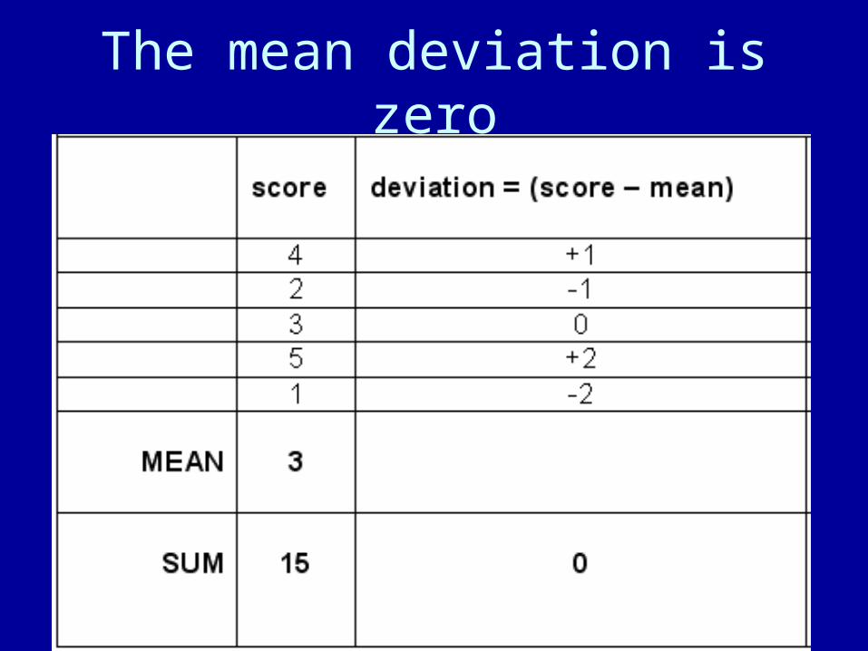
The mean deviation is zero

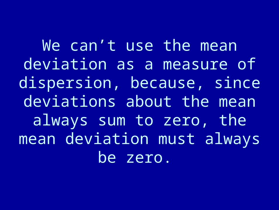
We can’t use the mean deviation as a measure of dispersion, because, since deviations about the mean always sum to zero, the mean

deviation must always be zero.

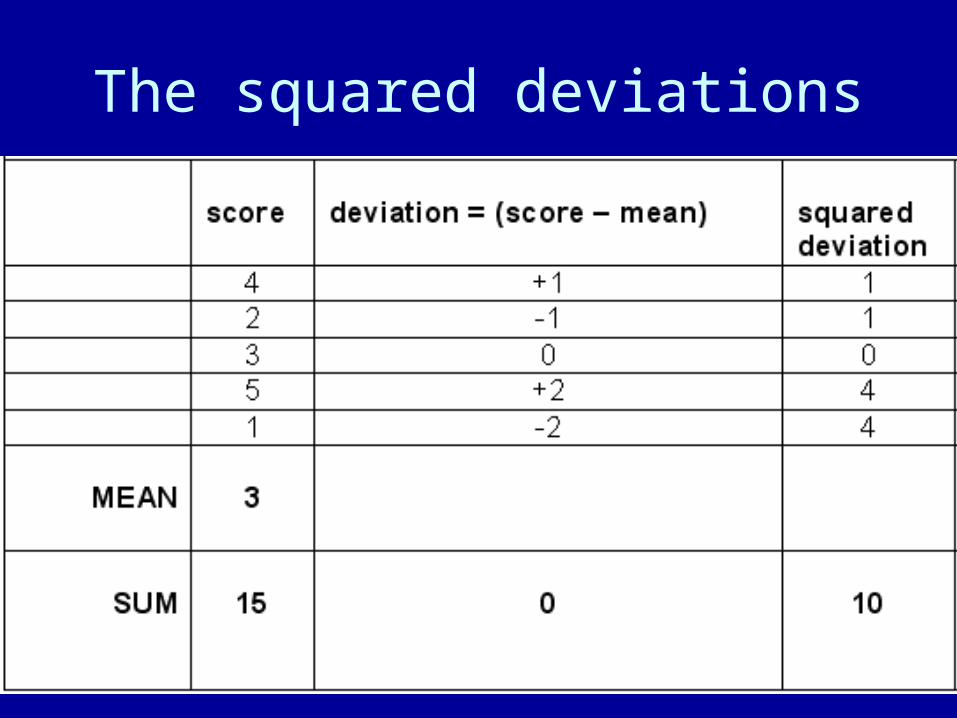
The squared deviations

The sum of the SQUARED deviations is always either positive (when scores have different values)

or zero (if all the scores have the same value).

The variance

• The variance is, essentially the MEAN SQUARED DEVIATION.

• But instead of dividing by the number of scores, divide by (number of scores ─ 1).

• Explanation later.

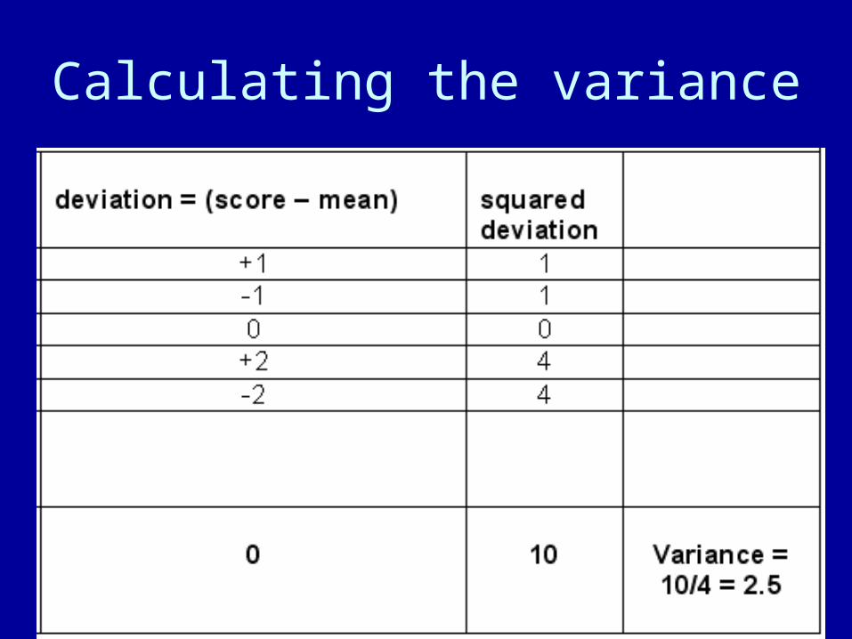
Calculating the variance

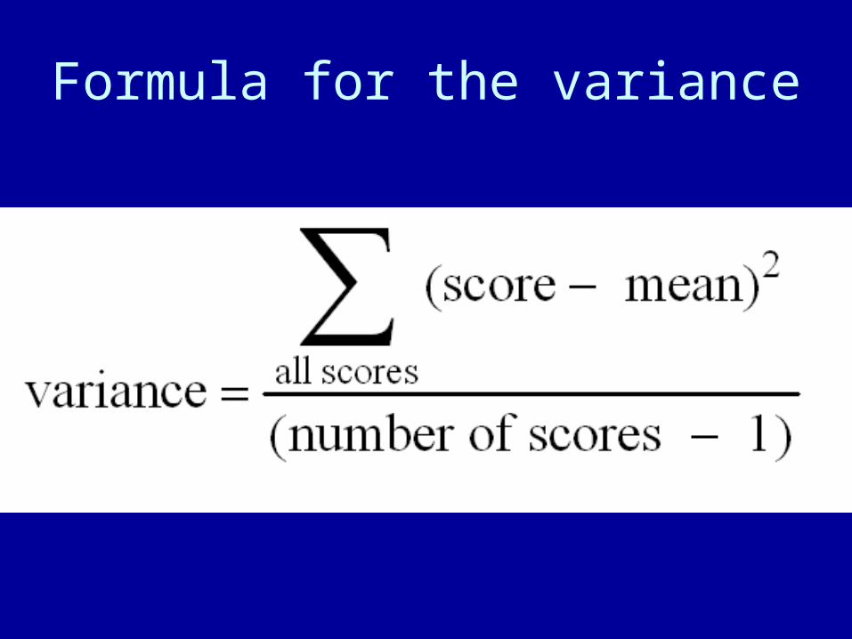
Formula for the variance

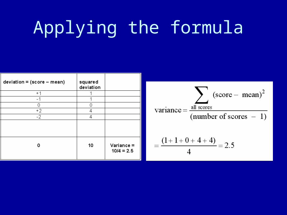
Applying the formula

A problem with the variance

• The simple range statistic has the merit of producing a score in the same units as the raw data.

• The variance, in squaring the deviations, produces squares of the original values and is therefore difficult to interpret.

• If you take the square root of the variance, you have the STANDARD DEVIATION, which is in the original units and easier to interpret.

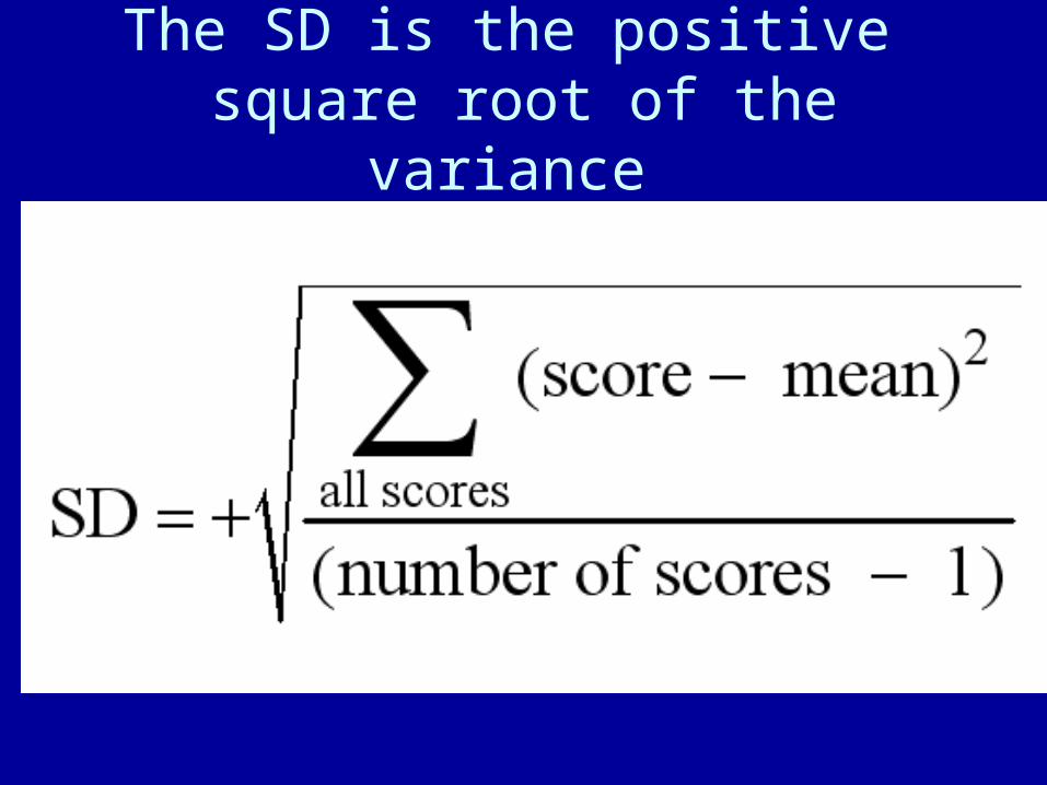
The SD is the positive square root of the variance

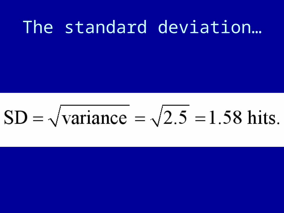
The standard deviation…