Lectures 9-10: Multiple Layer Perceptrons and Deep Network

Copyright © 2001-2018 K.R. Pattipati1

Fall 2018

November 12, 2018

Prof. Krishna R. Pattipati

Dept. of Electrical and Computer Engineering

University of Connecticut Contact: [email protected] (860) 486-2890

Lectures 9-10: Multiple Layer Perceptrons and Deep

Network Learning

mailto:[email protected]


• Duda, Hart and Stork, Chapter 6

• Murphy, Chapters 13 and 16

• Bishop, Chapter 5

• Theodoridis, Chapter 18

• Recent Papers on Deep Neural Networks

• T.J. Sejnowski, Deep Learning Revolution, MIT Press, 2018.

• Cited Papers on Deep Neural Networks

• Lectures 5 and 9 of Fei-Fei Li, Justin Johnson and Serena

Yeung http://cs231n.stanford.edu/syllabus.html

• 2016 lectures: CS 231: Convolutional Neural Networks for

Visual Recognition by Fei-Fei Li, Andrej Karpathy and Justin

Johnson

Reading List

http://cs231n.stanford.edu/syllabus.html


• Multiple Layer Perceptrons (MLPs)

• MLPs as Universal Approximators

• Back Propagation Algorithm

• Network Pruning

• Semi-supervised Learning of MLPs

• Introducing Deep Networks

– ReLU, Batch normalization, Dropout, Convolution, Max pooling, GPUs,

Stochastic Optimization

• Recurrent Neural Networks, LSTMs, GRUs, Transformer, 2D

Convolution Networks

• Summary

Lecture Outline


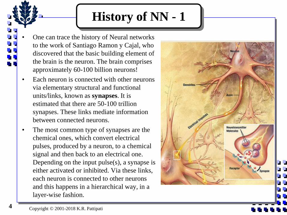
• One can trace the history of Neural networks

to the work of Santiago Ramon y Cajal, who

discovered that the basic building element of

the brain is the neuron. The brain comprises

approximately 60-100 billion neurons!

• Each neuron is connected with other neurons

via elementary structural and functional

units/links, known as synapses. It is

estimated that there are 50-100 trillion

synapses. These links mediate information

between connected neurons.

• The most common type of synapses are the

chemical ones, which convert electrical

pulses, produced by a neuron, to a chemical

signal and then back to an electrical one.

Depending on the input pulse(s), a synapse is

either activated or inhibited. Via these links,

each neuron is connected to other neurons

and this happens in a hierarchical way, in a

layer-wise fashion.

History of NN - 1


• In 1943, Warren McCulloch and Walter Pitts, developed a

computational model for the basic neuron linking neurophysiology

with mathematical logic. They showed that given a sufficient

number of neurons and adjusting appropriately the synaptic links,

each one represented by a weight, one can compute, in principle,

any computable function. As a matter of fact, it is generally

accepted that this is the paper that gave birth to the fields of neural

networks and artificial intelligence.

• Frank Rosenblatt borrowed the idea of a neuron model, as

suggested by McCulloch and Pitts, and proposed a true learning

machine, which learns from a set of training data. In its most basic

version, he used a single neuron and adopted a rule that can learn to

separate data, which belong to two linearly separable classes. That

is, he built a Pattern Recognition system. He called the basic neuron

a perceptron and developed a rule/algorithm, the perceptron

algorithm, which we discussed earlier and review it briefly.

History of NN - 2


Let us review what we have learnt so far

-- Rosenblatt’s Peceptron

Can categorize linearly separable classes

Perceptron

( , )y x w ( )g y z

z

1w

2w

pw

2x

px

1x

0w

1

-


A Single neuron can approximate a function (LMS)

Function Approximation

y zˆ( )g z

1w

2w

pw

2x

px

1x

0w

1

z

-

+


• Function can be binary for classification, but need not be.

• Training can be accomplished by sequential steepest descent (“LMS”), Incremental Gauss-Newton, SVM, and optimization techniques (Conjugate Gradient, Quasi Newton, Newton, . . . )

• Logistic comes naturally from Gaussian binary

classification problems. Softmax approximation in C-class case

• Also

1( )

1 yg y

e

)1( ggg

Function Approximation/Classification


• Are we done?

No. Consider the so-called “XOR problem” (parity problem,

Exclusive OR),

XOR Problem

21 xxt

Odd

parity

even

parity

x1 x2 t

0 0 0

0 1 1

1 0 1

1 1 0

(0,1)

(0,0)

(1,1)

(1,0) x1

x2

The two classes are not linearly separable. But, can

separate by two hyperplanes or a nonlinear discriminant.


Multiple Layer Perceptron for XOR Problem

1x

2x

Hidden Layer5.)1(

01 w

-1

5.)1(

02 w

1)1(

11 w

1)1(

12 w

1)1(

21 w

1)1(

22 w

(1)

1y

(1)

2y

Hidden Layer

(1)

1z

(1)

2z

1)2(

1 w

1)2(

2 w

5.)2(

0 w

-1

(2)z

-1

(1)

1 2 1

1ˆ

2z U x x

(1)

2 2 1

1ˆ

2z U x x

(2) (1) (1)

1 2

1ˆ ˆ ˆ

2z U z z


How Does it Classify it Correctly?

(1)

1 2 1

1ˆ

2z U x x

(1)

2 2 1

1ˆ

2z U x x

(2) (1) (1)

1 2

1ˆ

2z U z z

0 0 0 1 0

0 1 1 1 1

1 0 0 0 1

1 1 0 1 0

(1)

1z (1)

2z (2)z

Class 1 (o)

Class 2 (x)

Class 2 (x)

Class 1 (o)

0 0 0 0 0

1 0 0 1 1

0 1 0 1 1

1 1 1 1 0

(1)

1z (1)

2z (2)z

Class 1 (o)

Class 2 (x)

Class 2 (x)

Class 1 (o)

(1)

1 1 2ˆ 1.5z U x x

(1)

2 1 2

1ˆ

2z U x x

(2) (1) (1)

2 1

1ˆ ˆ ˆ2

2z U z z

Alternate solution


Geometric Interpretation

class 2class 1

class 1

(1) 1

1 2ˆ ˆ1 1( )z z

(1) 1

1 2ˆ ˆ0 1( )z z

(1) 1

1 2ˆ ˆ0 0( )z z

2x

1x

)1,0(

)0,1()0,0(

5.121 xx

)1,1(

5.021 xx

• Geometrically:


• Can extend it to n-bit parity problem

• In fact, any continuous function (or a set of functions ) can be approximated by a three layer perceptron (or a NN with a single hidden layer). This is called the universal approximation theorem, e.g.,

• An important corollary of this result is that, in the context of a classification problem, a method with sigmoidal nonlinearities and a hidden layer, can approximate any decision boundary to arbitrary accuracy e.g., 2–2–1 or

2–4–1 NN and 2–8–1 or 2–12–1 NN, for XOR problem.

MLP as Universal Approximator

yxf )(

(1) (2) (2) (1)

0 0

, ,pM

i ij j

i j

f y x w w g w g w x

yxf )(


Ideas of proof:

1. Any continuous function f(x) can be approximated by

piecewise step functions.

Universal Approximation of MLP-1

N

i

iii xxUfffxf0

10 )()()(

can approximate it as closely as desired by controlling

(or equivalently )

x

iii fff 1

several proofs that a NN with a single hidden

layer approximates a function or decision boundary

to arbitrary accuracy. Funahasi, Hecht-Nielson,

Cybenko, Hornik et al., Stinche Cormbe and White,

. . . .


2. Consider Fourier decomposition of in the

variable

similarly,

continuing,

Universal Approximation of MLP - 2

1( , ) pz x x

px

1 1 2 1( , ) ( , ) cos( )p p

p

p i p p p i

i

z x x A x x x i x

1

1

1

1 1 2 2 1 1( , ) ( , ) cos(

) cos( )

p p

p p

p p

p i i p p p

i i

i p p i

z x x A x x x i x

i x

1 1

1 2

1 ... 1 1( , ) cos( ) cos( )P p

p

p i i i p p i

i i i

z x x A i x i x


using repeatedly the trigonometric identity

Each of the cosine functions can be approximated by

piece-wise step functions. Since sigmoidal, tanh, etc.

approximate step functions, a two layer NN can

approximate a function to arbitrary accuracy.

)cos()cos(2

1coscos 212121

1 1

1

1

1

0 1:

( , ) cosp p

p

p k

k

p

p i i k k i i

n ki i i n

z x x C i x

Universal Approximation of MLP - 3


How to train MLPs with (L+1) layers of Perceptrons?

Inputs at layer 0 ~ we generally ignore this layer

Outputs at layer L

Most widely touted algorithm is the LMS algorithm, which

is called “Back propagation”.

Training MLPs

( 1)( 1)

0

ˆ ( ) output of

ˆ ˆ ˆ ( ( )) ( ) ( 1) ; ( )= ( ( ) )

th th

i

M ll

i ij j

j

z l i l layer or state at layer l

g y l g w l z l z l g W l z

2

1( ) (1 )

1

( ) tanh( ) ' (1 )

ii z

i i

If g z g g ge

If g z z g g


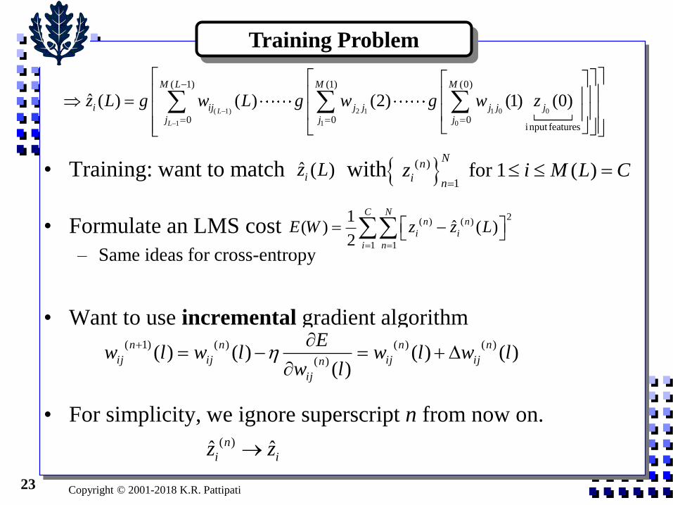
• Training: want to match with

• Formulate an LMS cost

– Same ideas for cross-entropy

• Want to use incremental gradient algorithm

• For simplicity, we ignore superscript n from now on.

ˆ ( )iz L ( )

1 for 1 ( )

Nn

in

z i M L C

2( ) ( )

1 1

1ˆ( ) ( )

2

C Nn n

i i

i n

E W z z L

( 1) 2 1 1 0 0

1 1 0

( 1) (1) (0)

0 0 0input features

ˆ ( ) ( ) (2) (1) (0)L

L

M L M M

i ij j j j j j

j j j

z L g w L g w g w z

)()()(

)()()()(

)(

)()1(lwlw

lw

Elwlw

n

ij

n

ijn

ij

n

ij

n

ij

Training Problem

( )ˆ ˆn

i iz z


( )

( ) ( )( ) ( )

( )

( ) ; (0) ( ) (0)

( ) (0) (0) ( ) ( )

( ) ( ) ( ); ( )

( ) ( ) ( )(0) (0) (0) ( ) ( )

f f

f

a t

a t a t t a t

f

f

a t

f f f

i i i i

Consider scalar equation x a x x given x t e x

J cx t ce x ce e x t x t t

t a t t c

J a a at ce x t x t t x t

: ( ); ( )( ) ( )

( ) ( )

( ) ( )

( ) ( ) ( ) ( ) ( ) ( ) ( ) ( ) ( ) ( )

So, to evaluate gradient, solve the forward equation for and b

i

f f

i i i

J JNote t x t

x t t

J J x t J t

x t t

a a at t x t t t t x t t t x t

x

ackward equation for

at any time ,and evaluate the gradient.t

Why Back Propagation?

Back propagation is

essentially a chain rule of

differentiation!( ) ( ( ( ( ))

; ;

g

f h f

g h

g g h f

L x L f h g x

L L f h g g

x f h g x x

L L f

f h h

L h

g g

x g h f L

g

x


• The sequential gradient is given by

Computing Gradient -1

ˆˆ ( ) ( )ˆ ˆ( ) ( ( )) ( 1); ( )

ˆˆ ˆ( ) ( ) ( ) ( ) ( )

i ii i j i

ij i i ij i

z l y lE E El g y l z l l

w l z l y l w l z l

• The key to back propagation is that can be computed

from . Indeed, are Lagrange

multipliers or co-states in optimal control theory. This

is also called the error signal. Let us see how it works.

At layer L,

Now consider at layer

)(li

( 1)

0( 1)

M l

j jl

)(li

ˆ( ) ( )ˆ ( )

i i i

i

EL z L z

z L

Note that E can be

any function of

ˆ and ( )

ˆ. ., ln[ / ]

ˆ| | ,1 2

i i i

R

i i

z z L

e g z z z

z z R

1,,2,1 LLl)(li

( 1)

0

ˆˆ ( 1) ( 1)( )

ˆˆ ˆ ˆ( ) ( 1) ( 1) ( )

M lj j

i

ji j j i

z l y lE El

z l z l y l z l

ˆ ˆij i iw y z

ˆˆ ˆ( ) { ( 1)} { ( 1)}i j jz l y l z l


So,

Or,

where

( 1)

0

ˆ( ) ( 1) ( ( 1)) ( 1)M l

i j j ji

j

l l g y l w l

ˆ( ) ( 1) ( ( 1)) ( 1) Tl W l Diag g y l l

matrix 1)(by 1)1(an is ][ lMlMwW ij

vector1)(an is )( lMl

vector1)1(an is )1( lMl

0

( 1)

ˆ( ( 1))

ˆ( ( 1))

ˆ( ( 1))M l

g y l

Diag g y l

g y l

an

diagonal matrix

1)1(by 1)1( lMlM

Computing Gradient -2


• Note: For l=L-1, the summation goes from 1 to M(L) = C

This recursive formula is the key to back propagation. It

allows the error signal (co-state) of a lower layer to

be computed as a linear combination of the error signals at

the layer (l+1), viz., . That is, the error signals

can be back propagated from L to 1.

Sometimes (most NN books including Bishop’s), one uses

the recursion then is:

with the terminal condition

)(li

)1( li

ˆ ( )ˆ( ) ( ) ( ( ))

ˆ ˆˆ( ) ( ) ( )

ii i i

i i i

z lE El l g y l

y l z l y l

( 1)

0

ˆ( ) ( 1) ( 1) ( ( ))M l

i j ji i

j

l l w l g y l

ˆˆ( ) ( ) ( ( ))i i i iL z L z g y L

Computing Gradient - 3

Nonlinearity

has local effect


• In matrix form:

• The weight update in matrix form is:

0

( )

ˆ( ( ))

( ) ( 1) ( 1)

ˆ( ( ))

T

M l

g y l

l Diag W l l

g y l

0

1 ( )

( )

ˆ( ( ))

ˆ( ) ( ) . ( ) ( 1)

ˆ( ( ))

Tn n n

M l

g y l

W l W l Diag l z l

g y l

( ) ˆ ( ) ( ) ( 1)Tn nW l l z l

Weight Matrix Update

Outer product


Algorithmically

1. Shuffle data

2. For Do

(i) Take data

(ii) Execute forward pass. Determine

and remember them.

(iii) Execute backward pass to evaluate

Update weights

End

3. Return to step 1

Training Algorithm in Brief

1

ˆ (0),N

n n n

nx z z

Nn ,,2,1

,n n

x z

ˆˆ ( ) and ( ( ))i iz l g y l

)(

and )(lw

El

ij

i


Graphically

Graphical Illustration

W

wBackward

PassForward

Pass

( ) ( )ˆ - ( )n n

i iz z L

( )ˆ( ) ( )n n n

i i iL z L z

ji

j

ji wgLL )()1(

Llayer

1layer L


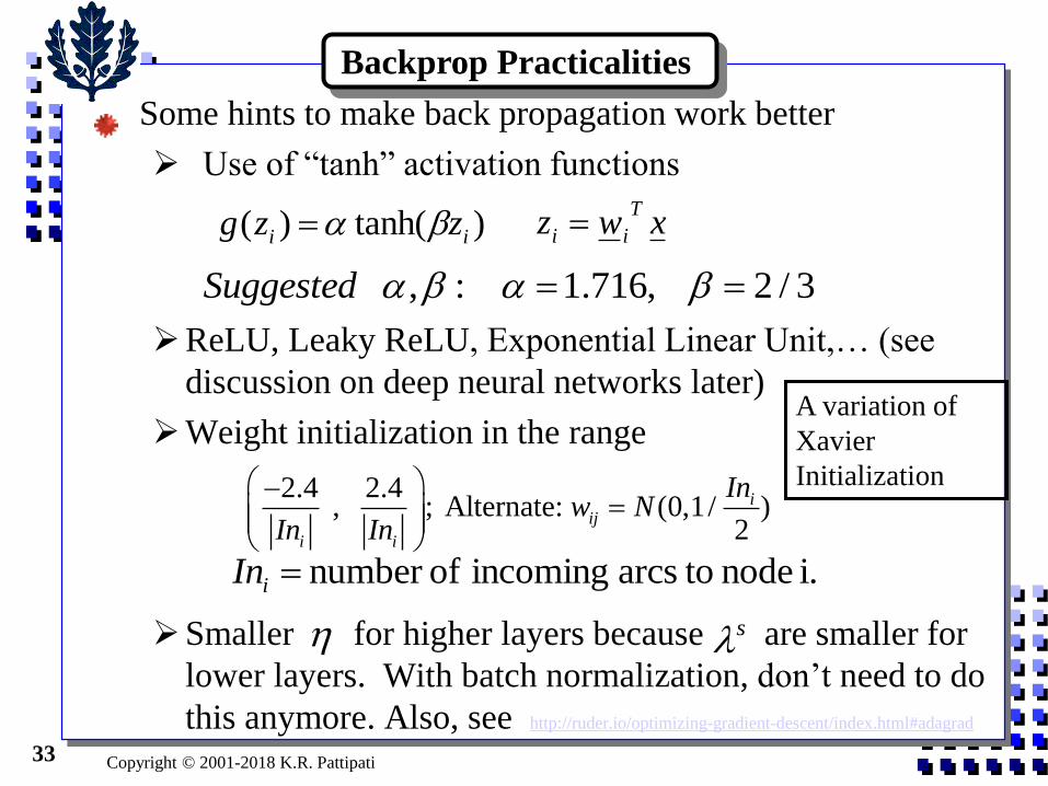
Some hints to make back propagation work better

Use of “tanh” activation functions

ReLU, Leaky ReLU, Exponential Linear Unit,… (see

discussion on deep neural networks later)

Weight initialization in the range

Smaller for higher layers because are smaller for

lower layers. With batch normalization, don’t need to do

this anymore. Also, see http://ruder.io/optimizing-gradient-descent/index.html#adagrad

Backprop Practicalities

)tanh()( ii zzg xwzT

ii

, : 1.716, 2 / 3Suggested

2.4 2.4 , ; Alternate: (0,1/ )

2

iij

i i

Inw N

In In

i. node toarcs incoming ofnumber iIn

s

A variation of

Xavier

Initialization

http://ruder.io/optimizing-gradient-descent/index.html#adagrad


Why [–1.716, 1.716] Range?

• g’(0) = 1.144

• linear range (-1, 1)

• extrema of g’’(.) near 1

-6 -4 -2 0 2 4 6-2

-1.5

-1

-0.5

0

0.5

1

1.5

2

y

g

g’

g’’


• Some hints to make training work better

Target values for Classes:

Minibatch averaged gradient. Typical batch sizes from 32 to 256.

Training with Noise: generate surrogate data with small noise added

(e.g., 0.1 variance for scaled data). Good for unbalanced case.

Training with hints: e.g., in fault diagnosis, add another output for the

fault severity during training only. Remove it for testing.

Randomized (Shuffled) training. Scale data to have zero mean and unit

variance or between (0.15 0.85) for sigmoid or (-1.716 1.716) for tanh

function. Use ReLU. Restart if training error does not decrease fast

enough. Multi-start

Minimum training set size N 10* number of weights

Perform cross validation or bootstrap. At worst, split N as follows:

65% Training; 10% Validation (use these to evaluate errors in

training); 25% Testing (should not be seen and used only once)

Network size from prediction error

Training Practicalities - 1

]1..111....111[ trageticlass

2 222; number of weights, variance of input noiseW

e W e

NEPE N

N N



Adaptive …. delta-bar-delta learning rule, quickprop, adagrad,…

NLP techniques: Conjugate gradient, Memoryless Quasi-Newton

method, MEKA. 2nd order methods need big batch sizes, like 10,000.

Regularization (Network pruning techniques) to improve

generalization. Build the simplest possible model or try to drive small

weights to zero

Weight eliminator


2

2

1 1 1

1ˆ( ) ( ) ( ) ; 0.001 0.1

2

C N Ln n

i i l l l e

i n l

E w z z L E w l

( ) ( 1)

2

2

1 1

( ) ... weight decay procedure or regularizationM l M l

l ij

i j

E w l w L

( 1) ( ) ( )

( )

ˆ ˆ( ) ( ) ( ) ( ( )) ( 1) ( )

ˆ = [1 ] ( ) ( ) ( 1)

n n n

ij ij i i j l ij

n

l ij i j

w l w l l g y l z l w l

w l l z l

12 2

( ) ( 1)

1 1 0 0

( ) 1M l M l

ij ij

l

i j

w wE w l

w w



Curvature-driven smoothing

• Network pruning … which weight should be set to zero

– Recall


2

21 1 1

ˆ ( )npN Ci

nn i j j

z L

x

1

2

1 1

ˆ (1 )

(1 ) (1 ) (2 1) ; (1 )

n

Nnn n

w

nE

N Nn nT nn n nT n

w

n n

E z z g g x

Q E g g g g E g x x x x x g g x

Add I if Q is not positive definite. The goal of optimal brain surgeon

(OBS) procedure is to set one of the weights to zero so as to minimize

the incremental increase in E.

21

1 1

1min . . 0

2

:[ ] 2[ ]

T T

ii i

i ii i

ii ii

J w Q w s t e w w

w wSolution w Q e J

Q Q

Zero out small weights

with large uncertainty


• Estimation Error is a function of (Barron, 1994)

Smoothness of the approximation function, Cf

Number of neurons, m

Number of Training Examples, N

Dimension of the input data, p

• Dropout; Srivastava, Nitish, et al. "Dropout: a simple way to prevent neural

networks from overfitting." Journal of machine learning research (2014)

• Normalization: Normalize activations of each layer (over a min-batch for

each node (feature) or over nodes (features) for each sample of a mini-

batch) to have same mean, and variance, 2 ( and are hyper

parameters). Alternately, normalize the weights of each layer:

• Early stopping: stop when validation error has not improved over n

iterations (n is called “patience”).

• Stochastic Gradient Descent is good for generalization


; optimize over and via SGD|| ||

VW g g V

V

( ) ( ln )f

error Training Error Generalization Error

C mpO O N

m N

https://www.cs.toronto.edu/~hinton/absps/JMLRdropout.pdf


• Nice to know uncertainty in predictions

• Parameter Posterior for Regression Case

• Predictive Posterior for Regression

• You can use EM-like algorithm to update {,}…. This is called

automatic relevance determination (ARD) …. A form of feature

selection

Predictive Posterior for Regression

2

21 1

1 2

1

1 1 1ˆ( ) ( ) ( ) ; output noise variance

2 2

At optimum

( | , , ) ( ; , ); ( ) ( ) ( ) ( ) ( )

ˆ( ) ( ) ( , )w

C NTn n th

i i i j i

i n i

Nn nT

MAP MAPw i j

n

n n n

MAPw

J w z z L w Diag w i

p w D N w w H H J w G x Diag G x Diag I

G x z L f x w Jacobian

1

ˆ( ) ( , ) ( , ) ( , ) ( )

( | , , , ) ( ; ( , ), ( ))

( ) (1/ ) ( , ) ( , )

T

MAP MAP MAPw

w

MAP z

T

MAP MAPz i w w

z x f x w f x w f x w w w

p z x D N z f x w x

x Diag f x w H f x w


• ARD via Regression

• Exploit the special structure of H in deriving gradients. We will revisit

this issue in the context of relevance vector machine (RVM).

Automatic Relevance Determination

1

2

1

ˆ( ) ( , ) ( , ) ( , )( )

( | , , , ) ( ; ( , ), ( ))

( ) (1/ ) ( , ) ( , )

( ) ( ) ( ) ( ) ( )

Assume ~ ( , ) and ~ ( ,

T

MAP MAP MAPw

MAP z

T

MAP MAPz i w w

Nn nT

MAPw i j

n

j j j i i

z x f x w f x w f x w w w

p z x D N z f x w x

x Diag f x w H f x w

H J w G x Diag G x Diag I

Ga a b Ga c d

1

1

1 1

)

Expected Negative log of posterior:

1( , ) {ln | ( ) | [ ( , )] ( )[ ( , )]}

2

( 1) ln ( 1) ln

i

Nn n n n n nT

MAP MAPz z

n

M C

j j j j i i i i

j i

l x z f x w x z f x w

a b c d


• Classification

Predictive Posterior for Classification

1

1 2

1

( ) ln ( , ) (1 ) ln(1 ( , ))

( , ) ( ( , ))... sigmoid function of ( , )

At optimum

( | ) ( ; , ); ( )

( ( , ) | , ) ( ( , ); ( , ), ( , ) ( , ))

( 1| ,

Nn nn n

n

n n n

MAP MAPw

T T

MAP w w

J w z g x w z g x w

g x w y x w y x w

p w D N w w H H J w

p g x w x D N g x w g x w g x w H g x w

P z x

1

( , )) ( )

( , ) ( , )1

8

MAP

T T

w w

g x wD

g x w H g x w

Cross entropy or

Deviance

Hedges against uncertainty


• L labeled and U unlabeled set of training examples

• Have side information (e.g., objects n and m are similar)

Semi-supervised Learning of MLPs

2

2

1 ; 0

ˆ( , )

ˆ ˆ|| ( , ) ( , ) || 1ˆ ˆ( ( , ), ( , ), )

ˆ ˆmax(0, || ( , ) ( , ) || ) 0

minimal margin between d

nm

n n

n m

n m nm

nm n m

nm

S if n and m are similar otherwise

Let z x W be output estimate for an input x

Define

z x W z x W if SL z x W z x W S

M z x W z x W if S

M

2

,

issimilar data

1ˆ ˆ ˆ( ) ( ) ( ( , ), ( , ), )

2

, 1 0.

n mn n

nm

n L n m U

nm nm

J W z z L L z x W z x W S

Optimize W via stochastic gradient by successively sampling from

labeled data unlabeled data with S and unlabeled data with S


• Extreme Learning Machines

Randomized projection of inputs to hidden layers

Linearly combine the outputs of hidden layers

• Convolutional Neural Networks (image processing/character recognition;

used in deep learning)

Series of convolutional and subsampling layers

o Local receptive fields and weight sharing: Inputs from a small region

(say 3x3 pixel patch) are mapped into next layer via sigmoid/ReLU

(same weights and bias) for all units

o Pooling: Subsampling takes small regions of convolution layers and

pools them (e.g., average, max value), scales it, adds a bias and

transforms via a nonlinearity, such as ReLU

Variations

0

0

( ) ( ); 1, 2,.., ; reasonably large;

, tanh, ,...; , are selected randomly

T

ii

i

h x g w x w i K K

g sigmoid rectifier w w

0 1

1

2

1

ˆ( ) ( );{ } selected to minimize

1ˆ ( ) Re ; , ,....

2 2

KT K

ii i i

i

Nn Tn n

n

z x v g w x w v

z z x v v gularized LS LASSO Elastic Net


• Training MLP is difficult if more than two hidden layers are used. The more layers

one uses, the more difficult the training becomes (unstable gradients) and

probability of getting stuck at local minima increases.

Is there any need for networks with more than two or three layers?

• The cortex of human brain can be seen as a multilayer architecture with 5-10 layers

dedicated only to our visual system (Hubel and Wiesel, 1962; also DL Rev. book)

• Using networks with more layers can lead to more compact representations of the

input-output mapping.

• Hastad switching lemma (1987) – Boolean circuits representable with a polynomial

number of nodes with k layers may require an exponential number of nodes with (k-

1) layers (e.g., parity) … more depth is better

– Deep networks may require less number of weights than a shallow representation

• Feature hierarchies (e.g., pixel edge texton motif part object in an

image recognition task) identified in deep networks can potentially be shared among

multiple tasks

– Transfer/Multi-task learning

• Currently DNN training is a painful “trial-and-error” process or uses genetic

algorithms or Bayesian optimization

Why Deep Networks?


What Made Deep Learning Feasible?

4

5

Deluge of data and ability to crowd source the labeling process for

supervisory learning …Availability of large scale (and often pre-trained)

labeled images (e.g., Alexnet, ImageNet, VGG16) and advances in cross-modal

(image, text/data, video and audio) representations…. “Big Data”

Availability of Graphics Processing Units (GPUs) that enable training of

very large image/text/speech datasets from several weeks to a few days

New nonlinearities (e.g., rectified linear units) and signal normalization that

avoid numerical problems associated with gradient computations

Convolution and max-pooling operations that exploit local connectivity to

reduce the dimension of the weight space, control overfitting and make the

network robust

Concept of dropout to realize an exponentially large ensemble of networks

from a single network

Advances in stochastic optimization, adversarial training and regularization

for robust network training

Features are learned rather than hand-crafted

More layers capture more invariances (Information-theoretic insights)


• Deep networks with sigmoid and tanh nonlinearities experience unstable

gradient problem

– Vanishing Gradient – recall saturation of sigmoids and tanh slow training

– Exploding gradient - products of many terms over layers unstable training

• One solution: Rectified Linear Units (ReLU) … easy to compute gradient

– g(y) = max (0,y). Note non-differentiability at y =0

– Leaky ReLU: set g(y) = ay for y 0 where a is small positive number ( 0.1)

– Exponential linear unit (ELU): set g(y) = (exp(y)-1) for y 0; 1

• Second Solution: Cross-entropy (Deviance) cost function avoids gradient

saturation

– Recall gradient does not have g’ and convexity of cross-entropy… Recall

ReLU and Cross-Entropy Avoid Unstable Gradient Problem

( 1)

0

ˆ( ) ( 1) ( 1) ( ( ))M l

i j ji i

j

l l w l g y l

2 '

1 1

{ ) &N N

T

n n nw n n w n

n n

J z g x J g x x


• Each node should interact with a small random set of other nodes

– At each iteration during training, each node is retained with a probability p

– During testing, the whole network is used, but the weights are scaled-down by p

(Google’s Tensorflow scales weights by 1/p and does not scale them during testing!)

– Essentially, dropout may be viewed as an ensemble of 2n networks (n = number of

nodes in the network) …. Better than weight decay regularization

Regularization using Dropout

Node present

with probability pw Node Always present

pw

During Training During Testing

p = 0.5 works!

( ) ( )

Approximation:

= node masking matrix

( ( ( 1) ( 1) )) ( ( 1) )l l

R

R

E g R l W l z g pW l z

Dropout does not help if

you have big data


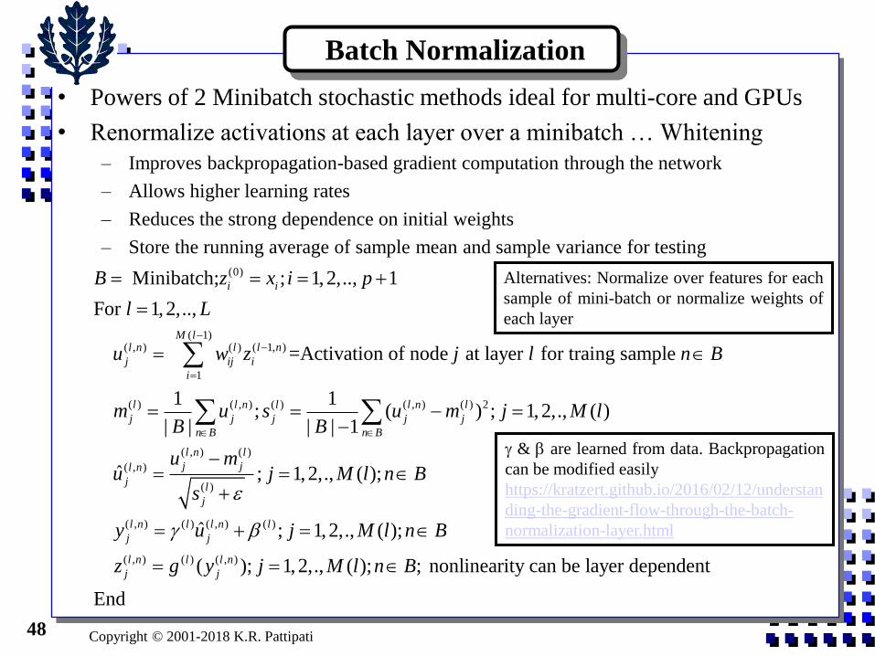
• Powers of 2 Minibatch stochastic methods ideal for multi-core and GPUs

• Renormalize activations at each layer over a minibatch … Whitening

– Improves backpropagation-based gradient computation through the network

– Allows higher learning rates

– Reduces the strong dependence on initial weights

– Store the running average of sample mean and sample variance for testing

Batch Normalization

(0)

( 1)( , ) ( ) ( 1, )

1

( ) ( , ) ( ) ( , ) ( ) 2

Minibatch; ; 1, 2,.., 1

For 1, 2,..,

=Activation of node at layer for traing sample

1 1; ( ) ; 1, 2,.,

| | | | 1

i i

M ll n l l n

j ij i

i

l l n l l n l

j j j j j

n B n B

B z x i p

l L

u w z j l n B

m u s u m j MB B

( , ) ( )

( , )

( )

( , ) ( ) ( , ) ( )

( , ) ( ) ( , )

( )

ˆ ; 1, 2,., ( );

ˆ ; 1, 2,., ( );

( ); 1, 2,., ( ); ; nonlinearity can be layer dependent

End

l n l

j jl n

jl

j

l n l l n l

j j

l n l l n

j j

l

u mu j M l n B

s

y u j M l n B

z g y j M l n B

& are learned from data. Backpropagation

can be modified easily

https://kratzert.github.io/2016/02/12/understan

ding-the-gradient-flow-through-the-batch-

normalization-layer.html

Alternatives: Normalize over features for each

sample of mini-batch or normalize weights of

each layer

https://kratzert.github.io/2016/02/12/understanding-the-gradient-flow-through-the-batch-normalization-layer.html


• Inspired by human’s visual system structure (local receptive fields,

weight sharing and pooling/aggregation)

• Much Faster to train (fewer weights)

• Recall convolution for one-dimensional discrete-time signals

• For two-dimensional signals (e.g., images), convolution operator is

• Most NN libraries use cross-correlation instead

• Key: W (receptive field) will have much smaller dimension than image

dimension X and W is shared smaller number of weights to learn.

You can have multiple W’s … called convolution kernels/filters/maps

– X is 32x32x3 and each W is 5 x 5x3 and 6 weight maps need to learn only

(5x5x3+1)x6=456 weight parameters to be learned

– You get 6 maps of 28x28x1 as outputs or 28x28x6 stacked maps….. (28=32-5+1)

– Connections: 76x6x28x28 =456x28x28=357,504 edges

Convolutional Networks

( ) ( )* ( ) ( ) ( ) ( ) ( )n n

s k x k w k x n w n k x n k w n

( , ) ( , )* ( , ) ( , ) ( , ) ( , ) ( , )m n m n

s i j x i j w i j x m n w i m j n x i m j n w m n

( , ) ( , )* ( , ) ( , ) ( , )m n

s i j x i j w i j x i m j n w m n


• What are the output volume sizes? F: filter size; N: input size; L: # Filters

– 32x32x3 image 6 5x5x3 convolution filters + ReLU 10 5x5x6 convolution filters

+ ReLU

– Output of first set of convolution filters: (N-F+1)x(N-F+1) x L=28x28x6

– Output of second set of convolution filters: 24x24x10

– Number of weight parameters: 456+1510=1966

• Typically, we move the filter one pixel at a time. What if we skip S

pixels called stride, S

– 32x32x3 image 6 5x5x3 convolution filters, stride 3+ ReLU 10 5x5x6

convolution filters, stride 1 + ReLU

– Output of first set of convolution filters: ((N-F)/S+1)x((N-F)/S+1) x L=10x10x6

– Output of second set of convolution filters: 6x6x10

– Stride 2 will not work in the first set of convolution filters because (32-5)/2+1=14.5

– Mostly, use stride, S=1; L is typically a power of 2

• In practice, common to zero pad the border with zeros. If pad with

P= (F-1)/2 zeros with stride, S=1 will not change the dimension spatially

– 32x32x3 image 6 5x5x3 convolution filters, stride 1, zero pad 2+ ReLU 10

5x5x6 convolution filters, stride 1, zero pad 2 + ReLU

– Output: 32x32x3 32x32x6 32x32x10

How Convolution Works with Strides and Zero Padding ?


Summary

• Convolution layer takes a volume I1 x J1 x K1 as input

• Convolution layer is parametrized by

– F: filter size

– L: # Filters

– S: Stride

– P: Amount of zero padding

• Produces a volume of I2 x J2 x K2 as output

• Number of weights per filter: F x F x K1 + 1 (for bias)

• Total Number of weights: (F x F x K1 +1)x L

• 1x1 convolution is perfectly OK to use

12

12

2

( 2 )1

( 2 )1

I F PI

S

J F PJ

S

K L

1 1( 2 ) ( 2 ): and must be divisible

I F P J F PNote

S S


• Y. LeCun, L. Bottou, Y. Bengio and P. Haffner,”Gradient-based Learning Applied to Document

Recognition, Proceedings of the IEEE, Vol. 86, No. 11, pp. 2278-2324, November 1998.

Example: LeNet 5

http://www.cs.cmu.edu/~aarti/Class/10701_Spring14/slides/DeepLearning.pdfC1,3,5: Convolutional layers

S2,4: Subsampling (pooling) layers

F6: Fully connected layer Layer Trainable Weights Connections (Edges)

C1 (25+1)x6 = 156 (25+1)x6x28x28 = 122,304

S2 (1+1)x6 = 12 (4+1)x6x14x14 = 5880 (2x2 links and bias = 5)

C3 6x(25x3+1) + 9x(25x4+1) + 1x(25x6+1) = 1516 1516x10x10 = 151,600

S4 16x2 = 32 16x5x5x5 = 2000 (2x2 links and bias = 5)

C5 120x(5x5x16+1) = 48,120 Same since fully connected MLP at this point

F6 84x(120+1) = 10,164 Same

Output 10x(84+1) = 850 (RBF) Same

60,850 weights

(instead of millions)

Max pooling is common. Other options: averaging, norm,….

http://www.cs.cmu.edu/~aarti/Class/10701_Spring14/slides/DeepLearning.pdf


Training Convolutional Networks

• Trained with BP, but with weight sharing

– Just average the weight updates over the shared weights in feature map layers

• Convolution layer

– A kxk receptive field would have a total of (k2 + 1) weights

– If a convolution layer had m feature maps, then only a total of (k2 + 1)m unique

weights to be trained in that layer (much less than a fully connected layer!)

• Sub-Sampling (Pooling) Layer

– Take maximum, average, norm, or weighted average of all elements of a receptive

filed. Result multiplied by one trainable weight and a bias added, then passed through

a non-linear activation function (e.g. ReLU) for each pooling node

– If a layer has m pooling feature maps, then 2m unique weights are to be trained

• The structure of the CNN is usually hand-crafted using trial and error

– Number of layers, number of receptive fields, sizes of receptive fields, sizes of sub-

sampling (pooling) fields, which fields of the previous layer to connect to, etc.

– Typically, decrease the size of feature maps and increase the number of feature maps

for later layers … typically by a factor of 2 every few layers


CNN’s Success in ImageNet Large Scale Visual Recognition Challenge

http://icml.cc/2016/tutorials/icml2016_tutorial_deep_residual_networks_kaiminghe.pdf

• ImageNet Classification Top-5 Error in Percentage

http://icml.cc/2016/tutorials/icml2016_tutorial_deep_residual_networks_kaiminghe.pdf


CNN Structures in Image Recognition Competitions - 1

• AlexNet, 8 Layers, top 5 error: 16.4% (2012), 1st used ReLU ~60M weights

– Input image 227x227x3

– 5 combined convolution and pooling layers: 11x11 convolution, 96 maps (conv 11-96)

max pool batch norm conv 5-256 max pool batch norm conv 3-384

conv3-384 conv 3-256 max pool batch norm

• Stride of 4 for first convolution kernel (,output (227-11)/4+1=55x55x96 and 11x11x96 parameters) and 1 for

the rest; Pooling layers with 3x3 receptive fields and stride of 2 throughout

– 2 fully connected (FC) layer with 4096 nodes

– Output layer with 1000 output nodes for classes

– https://papers.nips.cc/paper/4824-imagenet-classification-with-deep-convolutional-neural-networks.pdf

• ZFNet: 8 layers, top 5 error: 11.7% … hyper parameter tuning of AlexNet

– AlexNet with conv 11-96 stride 4 conv 7-96 stride 2; conv 3-384 conv 3-512; conv

3-384 conv 3-1024 and conv 3-256 conv 3-512

– https://arxiv.org/pdf/1311.2901.pdf

• VGG 19 layers, top 5 error: 7.3% (2014)

– 2 conv 3-64 max pool 2 conv 3-128 max pool 4 conv 3-256 max pool

4 conv 3-512 max pool 4 conv 3-512 max pool 2 FC 4096 FC 1000

softmax ….. 3x3 conv with 1 stride has less parameters and same effective receptive field

as 7x7 conv; Most memory in early layers and most weights in later FC layers


https://papers.nips.cc/paper/4824-imagenet-classification-with-deep-convolutional-neural-networks.pdf

https://arxiv.org/pdf/1311.2901.pdf






• GoogleNet, 22 Layers, top 5 error: 6.7% (2014),… called Inception-v1

– Conv 7-64 with stride 2 max pool 3/3 stride 2 Conv 3-192 max pool

3x3 stride 2

– Inception module: a good local network module with multiple parallel conv

filters (1x1, 3x3 and 5x5) and a 3x3 pooling operation. These are then

concatenated.

– No fully connected layers at the end

– Only 5M weights





• ResNet, 152 Layers, top 5 error: 3.57% (2015)

– Idea: Instead of training H(x) directly, train the residual F(x)= H(x) - x

– Stack residual blocks, 18 or 34 or 50 or 101 or 152 layers

– Every residual block has two 3x3 conv layers

– Periodically, double the number of maps and down sample using stride 2.

– At the beginning Conv 7-64 with stride 2 and 3x3 max pooling with stride 2

– No fully connected layers at the end




Current State of DNNs for Image Recognition

• Inception-ResNet-v2 by Google combines GoogleNet and ResNet ideas.

Inception-4 is the latest incarnation of GoogleNet






• Use of unsupervised learning to transform inputs into features that are easier to

learn by a final BP-based supervised model

• Often not a lot of labeled data available, while there may be lots of unlabeled

data. Unsupervised Pre-Training can take advantage of unlabeled data. Can be a

huge issue for some tasks.

• Q: Is there a training scheme that can get “good” local minima, which can then

be fine-tuned by BP?

– Approach 1: Pre-train each layer, via an unsupervised learning algorithm,

one layer at a time, in a greedy manner. The most popular approach is the

Restricted Boltzmann Machines (RBM).

– Approach 2: Replace layered RBMs with stacked auto-encoders. The latter

have been proposed as methods for dimensionality reduction. An auto-

encoder consists of two parts, the encoder and the decoder.

– The new CNN and BP-based deep network training has made these obsolete.

Early Methods of Training Deep Networks

1 20

1 20

: ( ); 1,2,.., ; .

ˆˆ: ( ); 1,2,.., , ; .

T

i ri e

T T

j pj d

Encoder h f w x w i r p W w w w

Decoder x g v h v j p V v v v W


• Autoregressive (AR) models: Predict the next term (word, phrase, expression,

label) in a sequence from a fixed number of previous ones using delay taps.

• Nonlinear Autoregressive Moving Average Models (NARMA) via MLPs:

MLPs with delayed inputs and outputs generalize autoregressive models with

nonlinear hidden units

• Nonlinear State space models

• Hidden Markov Models (Lecture 12).. need large # of states to model language

Dealing with Sequences

z2z1 zTz3…

y2y1 yTy3…

Viterbi algorithm

for inference and EM

(Baum-Welch)

algorithm for learning

1Hidden state evolution: ( , ); ~ input features at time step

Observations (output): ( , )

t t t t

t tt

z f z x x t

y h z x

1: 1: 1: 1: 1: 1 1

2 1

( , ) ( ) ( | ) ( ). ( | ) . ( | )T T

T T T T T t t t t

t t

p z y p z p y z p z p z z p y z


• Recurrent Neural Networks (RNNs): Introduce cycles into NN graph and the notion of

discrete time steps (epochs)

• RNNs can be unrolled in time as a DAG and apply Back Propagation

• How far to unroll? Typically less than 25 steps… initialize hidden variables from last unroll

• Often layers are stacked vertically (spatially) to obtain deep RNNs with different W

parameters at each layer. Back propagation still works.

• Recurrent networks are flexible: image captioning (CNNs feeding into RNNs), sentiment

classification, machine translation, video classification frame by frame, code generation,

Dealing with Sequences: RNNs

z

y

xt

1

1

Hidden state evolution: ( , ); ~ input vector at time

~ parameterized function..... same function at each time step !

: tanh( )

Observations (output):

t t t tW

W

t t tzz zx

tyzt

z f z x x t

f t

Example z W z W x

y W z

z0

x0

z1z2

x2 x2

y0 y1 y2• Since W parameters are the same at

each epoch, the gradients need to be

added over time epochs. Recall how

BP was introduced. Trivial concept if

you know optimal control!

• Has exploding or vanishing gradient

problem!

Good source on RNNs: A. Graves, “ Generating sequences with RNNs,” https://arxiv.org/pdf/1308.0850v5.pdf

https://arxiv.org/pdf/1308.0850v5.pdf


• Trick for vanishing and exploding gradient problem: Long Short-term Memory Networks

(Hochreiter and Schmidhuber, 1997).

• Long Short-term Memory Networks (LSTMs): use purpose-built memory cells to store

information and are better at finding and exploiting long range dependencies in data. Each

LSTM block contains one or more self-connected memory cells (c) and three multiplicative

units (input gate (i), output gate (o), forget/remember gate (f )). The cell remembers values

over arbitrary time intervals and the three gates regulate the flow of information into and out

of the cell.. It is like ResNet in skipping units. Back propagation still works.

Long Short-term Memory Networks

http://colah.github.io/posts/2015-08-Understanding-LSTMs/

1 1

1 1

1

1 0

1 tanh( )

); Hadamard produt ctanh(

t t

t t

t ffx fz fct

t t iix iz ic

tcx cz

t t oox oz c

t

tt t tt

tt

t t

W z c

W z c

W

f x W W b

i x W W b

c f c i x W

x W W c b

c

z

o W z

z o

Element-wiseSummation /Concatenation

Element-wisemultiplicationx t

z t-1

C t-1 z t

Ct

0

σ

+tanh

Inputs: outputs:

Input vector

Memory fromprevious block

Output ofprevious block

Memory fromcurrent block

Output ofcurrent block

Nonlinearities:

Sigmoid

Hyperbolictangent

Vector operations:

Bias:

x t

+ + + +0 1 2 3

z t-1

C t-1 Ct

z t

+

σ σ σtanh

tanh

z t

ft it

ot

Original source on LSTMs: S. Hochreiter and J. Schmidhuber, “Long Short-Term Memory,” Neural Computation, 9(8):1735-1780, 1997.

1. Forget gate decides whether previous cell state

should be kept or thrown out

2. Input gate decides what new information we will

store in the cell state

3. Cell state equation implements 1 and 2.

4. Output gate decides what should be in hidden state

5. Strength of cell state is encoded in tanh

http://colah.github.io/posts/2015-08-Understanding-LSTMs/


• LSTM without peepholes (i.e., where (f,i,o) gates are driven only by (xt, zt-1) )

perform reasonably well

• Forget and output gates are salient

• Start small, calibrate and build complex network models

• Gated Recurrent Unit (GRU)

– Merges forget and input gates into a reset gate

– Merges cell state and hidden state

– Fewer parameters and similar or better performance on some tasks

• LSTMs and GRUs can remember sequences of 100’s. For longer sequences,

recent variants are attention-based encoder-decoder (RNN, LSTM) models and

Causal 2D convolution networks (simultaneous source and target modeling)

• Attention-based models: e.g., Transformer : https://arxiv.org/pdf/1706.03762.pdf

– An attention model enables representation of context (e.g., focus on relevant text or image)

• 2D Convolutional Networks: https://arxiv.org/pdf/1808.03867.pdf

– Jointly encodes the source and target sequence in a 2D CNN

– It models context because each layer re-encodes the input in the context of the target sequence

Some Practical Observations and Recent Variants

1

1

1 1ta( ) n ( (h ))

t

tt

t

t t frx rz

t oox oz

ttzx zzt tt t

r x W b

x W b

z e o z o x W r

W z

o W z

W z




• Image classification (one-to-one): AlexNet, VGG19, VGG16, GoogleNet, ResNet,….

• Image captioning (one-to-many): https://arxiv.org/pdf/1411.4555v...

• Sentiment analysis (many-to-one): Sentence (a sequence) classified as expressing positive or

negative sentiment

• Machine Translation also known as sequence-to-sequence learning (e.g., English to French

Translation or many to many): https://arxiv.org/pdf/1409.3215.pdf

• Video to text (synced and sequenced input and output; many-to-many):

https://arxiv.org/pdf/1505.00487...

• Hand writing generation: http://arxiv.org/pdf/1308.0850v5...

• Image generation using attention models: https://arxiv.org/pdf/1502.04623...

• Question-answering: http://www.aclweb.org/anthology/...

Applications of LSTM and Attention-based Models

https://karpathy.github.io/2015/05/21/rnn-effectiveness/




http://arxiv.org/pdf/1308.0850v5.pdf


http://www.aclweb.org/anthology/P15-2116

https://karpathy.github.io/2015/05/21/rnn-effectiveness/


• Multiple Layer Perceptrons (MLPs)

• MLPs as Universal Approximators

• Back Propagation Algorithm

• Network Pruning

• Introducing Deep Networks

– ReLU, Batch normalization, Dropout, Convolution, Max

pooling, GPUs, Stochastic Optimization

• Semi-supervised Learning of MLPs

• RNNs, LSTMs, GRUs

Summary

Documents

Lectures 9-10: Multiple Layer Perceptrons and Deep Network