Lectures Notes of Robot Technology

Dr. W. Wahba i MTI, 2021

Modern University

For Information and Technology

Faculty of Engineering

Mechanical Engineering Department

Lectures Notes of

Robot Technology

MENG 308

Prepared By

Dr: Waleed A.M. Wahba

(First Edition 2021)

Dr. W. Wahba ii MTI, 2021

Dr. W. Wahba iii MTI, 2021

Contents Contents ......................................................................................................................................... iii

Chapter 1 Introduction .............................................................................................................. 1

1.1 Robot and Robotics .......................................................................................................... 2

1.2 What is an industrial robot required to do? ...................................................................... 2

1.3 Robot Manipulators .......................................................................................................... 3

1.3.1 Manipulators Components ........................................................................................ 4

1.3.2 Manipulators Classifications ..................................................................................... 5

1.4 Advantages and Disadvantages of Robots ....................................................................... 7

1.4.1 Robots Advantages ................................................................................................... 7

1.4.2 Robots Disadvantages ............................................................................................... 8

1.5 Asimov’s Laws of Robotics ............................................................................................. 8

Chapter 2 Robot Motion Description & Transformation ......................................................... 9

2.1 Robot Motion Degree-of-Freedom (DoF) ........................................................................ 9

2.1.1 Definition .................................................................................................................. 9

2.1.2 Grubler-Kutzbach Criterion .................................................................................... 10

2.1.3 Examples ................................................................................................................. 12

2.2 Robot Motion Description .............................................................................................. 13

2.2.1 Positions Description .............................................................................................. 13

2.2.2 Orientation Description ........................................................................................... 14

2.3 Robot Motion Transformation ....................................................................................... 18

Chapter 3 Forward Kinematics ............................................................................................... 20

3.1 Kinematic Chains ........................................................................................................... 20

3.2 Denavit-Hartenberg Representation ............................................................................... 22

3.2.1 Existence and uniqueness issues ............................................................................. 23

3.2.2 Assigning the coordinate frames ............................................................................. 25

3.3 Examples ........................................................................................................................ 27

3.3.1 Example 1: Three-Link Cylindrical Robot ............................................................. 27

3.3.2 Example 2: Spherical Wrist .................................................................................... 28

Dr. W. Wahba iv MTI, 2021

3.3.3 Example 3: Cylindrical Manipulator with Spherical Wrist .................................... 29

Chapter 4 Inverse Kinematics................................................................................................. 31

4.1 Inverse Kinematics Problem .......................................................................................... 31

4.2 Inverse Kinematics of a Serial Robot ............................................................................. 32

4.2.1 Kinematic Decoupling ............................................................................................ 33

4.2.2 Positioner’s Inverse Kinematics (Geometric Method) ........................................... 34

4.2.3 Wrist’s Inverse Kinematics ..................................................................................... 36

Chapter 5 Jacobian Matrix ...................................................................................................... 39

5.1 Speed Propagation Method to Compute the Jacobian Matrix ........................................ 42

5.2 Static of Robotic Manipulators ...................................................................................... 43

5.3 Singularities and Singular Configurations ..................................................................... 44

Chapter 6 References .............................................................................................................. 46

Dr. W. Wahba 1 MTI, 2021

Chapter 1

Introduction

Robotics and Mechatronics successfully fuse (but are not limited to) mechanics, electrical,

electronics, sensors and perception, informatics and intelligent systems, control systems and

advanced modeling, optics, smart materials, actuators, systems engineering, artificial intelligence,

intelligent computer control, precision engineering, virtual modeling, etc. into a unified framework

that enhances the design of products and manufacturing processes.

The synergy in engineering creative design and development enables a higher level of

interdisciplinary research that leads to high quality performance, smart and high functionality,

precision, robustness, power efficiency, application flexibility and modularity, improved quality

and reliability, enhanced adaptability, intelligence, maintainability, better spatial integration of

subsystems (embodied systems), miniaturization, embedded lifecycle design, sustainable

development, and cost effective approach. The adoption of such a synergized inter- or trans-

disciplinary approach to engineering design implies a greater understanding of the design process.

In the late 1970s, when robotics was going gangbusters, universities across the Midwest were

cranking out graduates with robotics engineering degrees. That was fine and good until the robotics

boom lost its luster in the 1980s. At the same time, Japanese companies started buying up robot

manufacturers. Engineers with a robotics engineering degree were suddenly out in the cold. The

universities teaching robotics gave the study a new name: mechatronics.

An automation and control method adopting integrated approach to technology has become

relevant to industries, machinery and consumer engineering products. Most of the domestic

equipment like automatic washing machines, automatic cameras, digital cameras, DVD players,


hard disc drives are examples of Mechatronic system which we use without bothering to know the

technology adopted in it.

1.1 Robot and Robotics The word robot represents a very general concept that is hard to define precisely, since this word

can be used to name a great number of machines.

Could you answer this question: which the following examples are robots?

1) Automatic camera?

2) Automatic washing machine?

3) Automatic dishwasher?

4) Automatic car (a car with an automatic gearbox)?

5) Crane?

For some people, some or all of these examples are kinds of robots, for others none of them are. It

all depends on what our own idea of what a robot is, and this can vary a lot from person to person.

The word robot is often related with some kind of machine that has similarities to some part of

human (or animal), body. But this is not always true.

Finely, Robot is an electromechanical device with multiple Degrees-of-Freedom (DoF) that is

programmable to accomplish a variety of tasks.

Close relationship with the concept of “automation”, the discipline that implements principles of

control in specialized hardware. Three levels of implementation:

• Rigid automation – factory context oriented to the mass manufacturing of products of

the same type. Uses fixed operational sequences that cannot be altered.

• Programmable automation – factory context oriented to low-medium batches of

different types of products. A programmable system allows for changing of manufacturing

sequences.

• Flexible automation – evolution of programmable automation by allowing the quick

reconfiguration and reprogramming of the sequence of operation. Flexible automation is

often implemented as “Flexible robotic work cells” (Decelle 1988, Pugh 1983).

Reprogramming/retooling the robots changes the functionality of the workcell.

Also, robot is an entity of sense, think, and act. For example, robot is a machine able to extract

information from its environment, and use this knowledge to move safely, in a meaningful and

purposive manner.

Robotics is the science of robots, while humans working in this area are called roboticists. Brady

1985, described robotics as the intelligent connection between perception and action. This is an

overly inclusive definition.

1.2 What is an industrial robot required to do? The purpose of an industrial robot is to repeat over and over the action of “quickly and efficiently

moving generic tools which are appropriate for a particular task to the location for that task”. For

example:


• In an arc welding operation, a welding torch (tool) attached to the tip of a robot

(manipulator) is required to move quickly and accurately to the welding site from the start

of the welding work to the position at the finish while instructions are given to the welding

device.

• As for handling work, a tool for picking up items that is attached to the tip of a robot

(manipulator) is given instructions to move to the site where the items to be moved are

placed, pick them up, and move them to a designated spot where the tool releases them in

a prompt and precise manner.

For these purposes, industrial robots need to be equipped with the basic capacities of speed—for

quick movement—as well as accuracy—to stop at the precise position required and to ensure that

they do not waver while they are on the move, and breadth for workable areas.

1.3 Robot Manipulators A robot manipulator is an electronically controlled mechanism, consisting of multiple segments,

that performs tasks by interacting with its environment. They are also commonly referred to as

robotic arms. Robot manipulators are extensively used in the industrial manufacturing sector and

also have many other specialized applications (for example, the Canadarm was used on space

shuttles to manipulate payloads). The study of robot manipulators involves dealing with the

positions and orientations of the several segments that make up the manipulators. This module

introduces the basic concepts that are required to describe these positions and orientations of rigid

bodies in space and perform coordinate transformations.


Figure 1.1, Robot manipulators configuration.

End-Effector

Figure 1.2, Manipulator components

1.3.1 Manipulators Components

Manipulators are composed of an assembly of links, joints, base, and end-effector, as shown in

Figure 1.2.

• Base can be either fixed in the work environment or placed on a mobile platform.

• Kinematic open chain composed of:

o Links are defined as the rigid sections that make up the mechanism and

o Joints are defined as the connection between two links.

• End effector is the device attached to the manipulator which interacts with its environment

to perform tasks is called the end-effector.

Joints allow restricted relative motion between two links. The following Table describes

five types of joints.

Joint Name Drawing Discerption

Linear

(Prismatic)

Joint

(P)

➢ Allows translation between two links.

➢ It is represented by symbol P.

➢ The joint variable is displacement d.

Rotary

(Revolute)

Joint

(R)

➢ Allows rotation between two links.

➢ It is represented by symbol R.

➢ The joint variable is angle θ


Spherical

Joint

(S)

➢ Allows rotation around three axes.

➢ It is represented by symbol S.

➢ The joint variables are θ, γ and ψ.

Universal

Joint

(U)

➢ Allows rotation around two axes.

➢ It is represented by symbol U.

➢ The joint variables are θ1 and θ2.

Cylindrical

Joint

(C)

➢ Allows rotation and translation.

➢ It is represented by symbol C.

Screw

Joint

(SC)

➢ Allows rotation and a constrained

translation.

➢ It is represented by symbol SC.

Prismatic and Revolute are the two common joints in serial robot manipulators

1.3.2 Manipulators Classifications

Manipulators can be classified according to a variety of criteria. We will discuss two of these criteria:

1.3.2.1 Motion Characteristics

1) Cartesian manipulator: have a simple structure of two or three sliding axes where the

sliding axes are joined together. While they are unable to perform complicated movements,

their precision level is high, and they are easy to control, making them appropriate for use

in the areas of semiconductors, healthcare, or chemicals for tasks such as the assembly of

small parts or outfitting electronic circuits.

2) Cylindrical and polar manipulator: consist of structures that were first used for

industrial robots in the early years. While their field of operation is broad, they aren’t very

suitable for complicated tasks that require them to make roundabout movements. The arm

of cylindrical Robots rotates vertically and expands and contracts from the pivotal axis.


Meanwhile, the arm of Polar Robots moves vertically, expands, and contracts from the

pivotal axis.

3) Spherical manipulator: A manipulator is called a spherical manipulator if all the links

perform spherical motions about a common stationary point.

4) Spatial manipulator: A manipulator is called a spatial manipulator if at least one of the

links of the mechanism possesses a general spatial motion.

RRR Polar Manipulator

PRR Cylindrical

Manipulator

RRP Spherical Manipulator

RRR (3R) Spherical

Manipulator

PPP Cartesian manipulator

Spatial Manipulator

1.3.2.2 Kinematic Structure

1) Open-loop manipulator (or serial robot): A manipulator is called an open-loop manipulator if its links form an open-loop chain.

2) Parallel manipulator: A manipulator is called a parallel manipulator if it is made up of a closed-loop chain.

3) Hybrid manipulator: A manipulator is called a hybrid manipulator if it consists of open loop and closed loop chains.


1.3.2.3 JIRA Classification

According to the Japanese Industrial Robot Association (JIRA), robots can be classified as follows:

Class 1: manual handling device – a device with several DOF’s actuated by the operator.

Class 2: fixed sequence robot – similar to fixed automation.

Class 3: variable sequence robot – similar to programmable automation.

Class 4: playback robot – the human performs tasks manually to teach the robot what

trajectories to follow.

Class 5: numerical control robot – the operator provides the robot with the sequence of tasks

to follow rather than teach it.

Class 6: intelligent robot – a robot with the means to understand its environment, and the

ability to successfully complete a task despite changes in the surrounding

conditions where it is performed.

1.4 Advantages and Disadvantages of Robots

1.4.1 Robots Advantages

1) Robotics and automation can, in many situations, increase productivity, safety, efficiency,

quality, and consistency of products

2) Robots can work in hazardous environments

3) Robots need no environmental comfort

4) Robots work continuously without any humanity needs and illnesses


5) Robots have repeatable precision at all times

6) Robots can be much more accurate than humans, they may have milli or micro inch

accuracy.

7) Robots and their sensors can have capabilities beyond that of humans

8) Robots can process multiple stimuli or tasks simultaneously, humans can only one.

9) Robots replace human workers who can create economic problems

1.4.2 Robots Disadvantages

1) Robots lack capability to respond in emergencies, this can cause:

• Inappropriate and wrong responses

• A lack of decision-making power

• A loss of power

• Damage to the robot and other devices

• Human injuries

2) Robots may have limited capabilities in

• Degrees of Freedom

• Dexterity

• Sensors

• Vision systems

• Real-time Response

3) Robots are costly, due to

• Initial cost of equipment

• Installation Costs

• Need for peripherals

• Need for training

• Need for Programming

1.5 Asimov’s Laws of Robotics Asimov developed three laws of robotics to cope with potential for robots to harm people. These

laws are simple and straightforward, and they embrace the essential guiding principles of a good

many of the world’s ethical systems.

First law (Human safety): A robot may not injure a human being, or, through inaction, allow

a human being to come to harm.

Second law (Robots are slaves): A robot must obey orders given it by human beings, except

where such orders would conflict with the First Law.

Third law (Robot survival): A robot must protect its own existence as long as such protection

does not conflict with the First or Second Law.

Hint: They are extremely difficult to implement!!! Why?


Chapter 2

Robot Motion Description & Transformation

A robot/manipulator can be schematically represented from a mechanical viewpoint as kinematic

chain of rigid bodies (links) connected by means of revolute or prismatic joints. One end of the

chain is fixed to a base, while an end-effector is attached on the other end.

Robot arm kinematics deals with the analytical study of the geometry of motion of a robot arm

with respect to a fixed reference coordinate system as a function of time without regard to the

forces / moments that cause the motion. Kinematic equation gives the relationship between the

joint displacement and the position and orientation of end-effector is determined. Determining the

final position & orientation of the end effector depending upon the joint angles is known as forward

kinematics and finding the joint angles depending upon the position of end effector is known as

inverse kinematics.

2.1 Robot Motion Degree-of-Freedom (DoF)

2.1.1 Definition

The stably independent motion capability of a mechanism or kinematic chain is defined as its

degree of freedom or mobility. This capacity includes the following three aspects:

1) In magnitude, this capacity represents the number of independent coordinates

needed to define the configuration of a kinematic chain or mechanism.

2) In property, this capacity represents the mobility to be:

• rotational or translational


• full and continuous airspace or discrete

3) The mobility in space-time is instantaneous or full-cycle.

The “stably” in the definition means that the magnitude and property all have a stably finite motion

area and that the area is not infinite or discrete. In this case, the mobility is full-cycle. The mobility,

which only exists on an infinitesimal area, is not the mobility of mechanism that we recognize.

In this chapter, the second and third items are proposed for spatial multi-mobility mechanisms and

parallel mechanisms. Different mobility mechanisms have different applications. For example:

• some printer localizers need to use a planar two-dimension translation mechanism only;

the space localizer needs a three-dimension translation mechanism;

• a Robot SCARA needs three-dimension translation and one-dimension rotation space

mechanism;

• a weld robot needs three-translational and two-rotational kinematic capacities, etc.

The parallel mechanisms can be classified by its mobility property. For example, the two-DOF

parallel mechanisms can be classified into three categories: RR, PP, and RP, where R denotes

rotational freedom and P denotes translational freedom. This means that the output link of the two-

DOF parallel mechanisms may have two rotational freedoms, two translational freedoms or one

rotational, and one translational freedom, respectively. For spatial mechanisms, there are 12 kinds

of freedom by mobility property, as shown in next Table.

Number of mobility Mobility property

2 RR, RP, PP

3 RRR, PPP, RRP, PPR

4 RRRR, TTTT, RRRP,

5 RRRPP, PPPRR

2.1.2 Grubler-Kutzbach Criterion

Obtaining the number of degrees of freedom (DoF), also known as mobility for a mechanism, is

one of the most basic topics in the field of mechanism. Formally, the degree of freedom (DoF) of

a mechanical system is defined as the number of independent coordinates or minimum coordinates

required to fully describe its position or configuration. Thus, a rigid body moving in the three-

dimensional Cartesian space has six-DoF, next Figure, three each for position and orientation.

Several methodologies exist to determine the DoF. One such method is given by Grubler in 1917

for planar mechanisms, which is later generalized by Kutzbach in 1929 for spatial mechanisms.

Commonly, they are known as Grubler-Kutzbach criterion (G-K formula). This criterion, which is


based on a simple arithmetic, is successful in analyzing almost all of the planar mechanisms and

some spatial mechanisms. Hence, the criterion has become very popular, and a great number of

engineers use it in practice.

Since robots consist of rigid bodies, DoF can be expressed as follows:

DoF = (sum of freedoms of the bodies) − (number of independent constraints).

A joint can be viewed as providing freedoms to allow one rigid body to move relative to another.

It can also be viewed as providing constraints on the possible motions of the two rigid bodies it

connects. For example, a revolute joint can be viewed as allowing one freedom of motion between

two rigid bodies in space, or it can be viewed as providing five constraints on the motion of one

rigid body relative to the other. Generalizing, the number of degrees of freedom of a rigid body

(three for planar bodies and six for spatial bodies) minus the number of constraints provided by a

joint must equal the number of freedoms provided by that joint.

The freedoms and constraints provided by the various joint types are summarized in the next Table.

Consider a mechanism consisting of N links, where ground is also regarded as a link. Let:

• J be the number of joints,

• m be the number of degrees of freedom of a rigid body (m = 3 for planar mechanisms and

m = 6 for spatial mechanisms),

• fi be the number of freedoms provided by joint i, and

• ci be the number of constraints provided by joint i, where fi + ci = m for all i.

Then,


This formula holds in “generic” cases, but it fails under certain configurations of the links and

joints, such as when the joint constraints are not independent.

2.1.3 Examples

1) (Four-bar linkage and slider–crank mechanism). The planar four bar linkage shown in next

Figure consists of four links (one of them ground) arranged in a single closed loop and

connected by four revolute joints. Since all the links are confined to move in the same

plane, we have m = 3.

Substituting N = 4, J = 4, and fi = 1, i = 1, . . . , 4, into G-K formula, we see that the four-

bar linkage has one degree of freedom.

2) The slider–crank closed-chain mechanism, in Figure below, can be analyzed in two ways:

a) the mechanism consists of three revolute joints and one prismatic joint (J = 4 and each

fi = 1) and four links (N = 4, including the ground link), or

b) the mechanism consists of two revolute joints (fi = 1) and one RP joint (the RP joint is

a concatenation of a revolute and prismatic joint, so that fi = 2) and three links (N = 3;

remember that each joint connects precisely two bodies).

In both cases the mechanism has one degree of freedom.

3) (A planar mechanism with overlapping joints). The planar mechanism illustrated, in Figure

below, has three links that meet at a single point on the right of the large link.

Recalling that a joint by definition connects exactly two links, the joint at this point of

intersection should not be regarded as a single revolute joint. Rather, it is correctly

interpreted as two revolute joints overlapping each other. Again, there is more than one

way to derive the number of degrees of freedom of this mechanism using G-K formula:

a) The mechanism consists of eight links (N = 8), eight revolute joints, and one

prismatic joint. Substituting into G-K formula yields:

DoF = 3(8 − 1 − 9) + 9(1) = 3


b) Alternatively, the lower-right revolute–prismatic joint pair can be regarded as a

single two-DoF joint. In this case the number of links is N = 7, with seven revolute

joints, and a single two-dof revolute–prismatic pair. Substituting into G-K formula

yields:

DoF = 3(7 − 1 − 8) + 7(1) + 1(2) = 3

4) (Delta robot). The Delta robot in next Figure consists of two platforms.

The lower one mobile, the upper one stationary – connected by three legs. Each leg contains

a parallelogram closed chain and consists of three revolute joints, four spherical joints, and

five links. Adding the two platforms, there are N = 17 links and J = 21 joints (nine revolute

and 12 spherical). By G-K formula:

DoF = 6(17 − 1 − 21) + 9(1) + 12(3) = 15

These 15 degrees of freedom, however, only three are visible at the end-effector on the

moving platform.

In fact, the parallelogram leg design ensures that the moving platform always remains

parallel to the fixed platform, so that the Delta robot acts as an x–y–z Cartesian positioning

device. The other 12 internal degrees of freedom are accounted for by torsion of the 12

links in the parallelograms (each of the three legs has four links in its parallelogram) about

their long axes.

2.2 Robot Motion Description Robot motion description focuses on description of positions, of orientations, and of an entity that

contains both of these descriptions the frame. Description is used to specify attributes of various

objects with which a manipulation system deals. These objects are parts, tools, and the manipulator

itself. In this section.

2.2.1 Positions Description

Once a coordinate system is established, we can locate any point in the universe with a 3 x 1

position vector. Because we will often define many coordinate systems in addition to the universe

coordinate system, vectors must be tagged with information identifying which coordinate system

they are defined within. In this book, vectors are written with a leading superscript indicating the


coordinate system to which they are referenced (unless it is clear from context)—for example, Ap

This means that the components of Ap have numerical values that indicate distances along the

axes of {A}.

Each of these distances along an axis can be thought of as the result of projecting the vector onto

the corresponding axis. Figure above, pictorially represents a coordinate system, {A}, with three

mutually orthogonal unit vectors with solid heads. A point Ap is represented as a vector and can

equivalently be thought of as a position in space, or simply as an ordered set of three numbers.

Individual elements of a vector are given the subscripts x, y, and z:

2.2.2 Orientation Description

As seen in section before, position is represented as three values: Px , Py , Pz in x, y, z coordinates.

This is intuitive and easy to understand. It may not be difficult also to understand the physical

orientation of the robot. However, the orientation should be represented as numerical values to

control the robot and it is challenging to understand. In robotics, the orientation is represented by

using the following rotation concepts:

1) Rotation matrix

2) Euler angles

3) Axis-angle representation

4) Quaternion

The advanced use of robot orientation is needed for applications including but not limited to:

1) 3D vision

2) Multi-robot coordination

3) Advanced palletizing

4) Offline programming

5) Welding

2.2.2.1 Rotation matrix

In linear algebra, a rotation matrix is a matrix that is used to perform a rotation in Euclidean space.

For Let us get started with the rotation in two dimensions. In the figure below, corresponding to

the frame {𝑖}, the X and Y unit direction vectors of the frame {𝑗} are:


Rotation from the frame {𝒊} to {𝒋}

Projection:

Here, the rotation matrix from the frame {𝑖} frame {𝑗} is:

As an example, let, the frame {𝟏} is rotated with 𝜋 from the frame {0}. Then the rotation matrix is:

A position with the coordinates (4, 3) in the frame {0} can be calculated to the coordinates in the frame {1} by using

the rotation matrix.

As shown in the example of two-dimensional rotation matrix, the rotation matrixis determined by

the unit directions vectors in the reference frame. In addition, the rotation matrix is useful to

calculate the position and orientation values in different coordinate systems. Note that a coordinate

system is composed of an origin and a frame, the directions of axes. In robotics, we use the three-

dimensional (3-by-3) rotation matrix.

However, it is inconvenient to use 9 numerical values to represent the orientation. Therefore, other

ways are also used to represent the orientation.

2.2.2.2 Euler angles

The Euler angles are three angles introduced to describe the orientation of rigid body with respect

to a fixed coordinate system.5 Any orientation can be achieved by composing three elemental

rotations about the axes of a coordinate system. To be specific, rotate the angles of γ,β and α along

the X, Y and Z axes from the reference frame, respectively then you will achieve the orientation.

In the figure 5, the reference frame is shown in blue and the rotated orientation is shown in red.

The angles γ, β, α can also be called RPY (Roll, Pitch and Yaw).


Proper Euler angles geometrical definition

The Euler angles are used to understand the robot orientation, but it should be converted to the rotation matrix for

calculations such as kinematics and dynamics. Given Euler angles γ, β, α, the rotation matrix can be calculated by the

following equations:

For a given rotation matrix R, the Euler angles are determined as follows:

Advantages & Disadvantages

The Euler angles are preferred because only three values are needed and geometrically easy to

understand compared to other methods.

However, there are two critical disadvantages in this representation.

1) The values are not continuous so that calculations with the Euler angles are complicated.

2) In addition, the final orientation depends on the sequence of rotations. In other words, even

with the same amounts of roll, pitch and yaw, the orientations will be different whether it

is rotated with roll first or yaw first, which is confusing.

2.2.2.3 Rotation vector

The axis-angle representation parameterizes a rotation in the linear space by:


• Unit vector 𝑢 indicating the direction of an axis of rotation, and

• Angle 𝜃 describing the magnitude of the rotation about the axis.

The axis-angle representation can define the

relationship between two orientations. For example, in

the Figure below, the blue orientation can be rotated

by the angle 𝜃 along the direction vector 𝑢 to the red

orientation.

Axis-angle representation

If we have a fixed reference frame, can call it the base frame, we can represent any orientation by

four numbers: three elements for the unit direction vector and an angle.

If we multiply the angle to each element of the unit direction vector, we can reduce to the three

numerical values, which we can call the rotation vector, as follows:

The axis-angle representation is useful in the robot control because it is free from continuity and

rotational sequence issues, which was the limitations of the Euler angles.

However, it is hard to match between the physical orientation and the numerical values of the

rotation vectors. In some softwires like UR robots, use the rotation vector to represent the

orientation of the robot pose.

To convert to the rotation matrix, the rotation vector should be divided into the angle and unit

direction vector.

Where: c = cos𝜃 , s = sin𝜃 , and C = 1−cos𝜃

For a given rotation matrix R, the rotation vector can be calculated as follows:


2.3 Robot Motion Transformation You may need to move the robot from the current position with the certain amount in position and

orientation. Given a current position and changes of position and orientation, the target position

can be calculated as follows:

The movement in position can be called translation and that in orientation can be represented by

rotation. In robotics, both translation and rotation can be combined and mathematically represented

as the transformation 4x4 matrix as below:

This is a partitioned matrix with R a 3 × 3 rotation matrix and t a three-dimensional (3-D) column

vector corresponding to the translation; note that the 0 in the bottom left corner really represents a

row of three zeros.

This representation of a rigid transformation is sometimes called the homogeneous representation

because of connections with projective geometry, but projective geometry will not be considered

here. To model the effect of such a transformation on a point, we need to change our representation

of points. From now on, a point with coordinates (x, y, z) will be represented by a four-dimensional

(4-D) column vector:

The transformation matrix can be used not only for the movement but also to represent a pose. The

above example to move from a current pose with changes of position and orientation can be

represented by the transformation matrix as below.

Where, inverse is just the inverse of the pose transformation matrix as below:



Chapter 3

Forward Kinematics

For the purpose of controlling a robot, it is necessary to know the relationships between the joints

motion (input) and the end-effector motions (output), because the joint motions control the end-

effector movements. Thus, the study of kinematics is important, where transformations between

the coordinate frames attached to different robot links of the robot need to be performed

Forward or configuration kinematics problem is concerned with the relationship between the

individual joints of the robot manipulator and the position and orientation of the tool or end-

effector. Stated more formally, the forward kinematics problem is to determine the position and

orientation of the end-effector, given the values for the joint variables of the robot. The joint

variables are the angles between the links in the case of revolute or rotational joints, and the link

extension in the case of prismatic or sliding joints. The forward kinematics problem is to be

contrasted with the inverse kinematics problem, which will be studied in the next chapter, and

which is concerned with determining values for the joint variables that achieve a desired position

and orientation for the end-effector of the robot.

3.1 Kinematic Chains As described in Chapter 1, a robot manipulator is composed of a set of links connected together

by various joints. The joints can either be very simple, such as a revolute joint or a prismatic joint,

or else they can be more complex, such as a ball and socket joint. (Recall that a revolute joint is


like a hinge and allows a relative rotation about a single axis, and a prismatic joint permits a linear

motion along a single axis, namely an extension or retraction.) The difference between the two

situations is that, in the first instance, the joint has only a single degree-of-freedom of motion: the

angle of rotation in the case of a revolute joint, and the amount of linear displacement in the case

of a prismatic joint. In contrast, a ball and socket joint has two degrees-of-freedom. In this book it

is assumed throughout that all joints have only a single degree-of-freedom. Note that the

assumption does not involve any real loss of generality, since joints such as a ball and socket joint

(two degrees-of-freedom) or a spherical wrist (three degrees-of-freedom) can always be thought

of as a succession of single degree-of-freedom joints with links of length zero in between. With

the assumption that each joint has a single degree-of-freedom, the action of each joint can be

described by a single real number: the angle of rotation in the case of a revolute joint or the

displacement in the case of a prismatic joint. The objective of forward kinematic analysis is to

determine the cumulative effect of the entire set of joint variables.

Coordinate frames attached to elbow manipulator

A robot manipulator with n joints will have n+1 links, since each joint connects two links. We

number the joints from 1 to n, and we number the links from 0 to n, starting from the base. We

will consider the location of joint i to be fixed with respect to link i−1. When joint i is actuated,

link i moves. Therefore, link 0 (the first link) is fixed, and does not move when the joints are

actuated. With the ith joint, we associate a joint variable, denoted by qi. In the case of a revolute

joint, qi is the angle of rotation, and in the case of a prismatic joint, qi is the joint displacement:

Now suppose Ai is the homogeneous transformation matrix that expresses the position and

orientation of oixiyizi with respect to oi-1xi-1yi-1zi-1. The matrix Ai is not constant, but varies as the

configuration of the robot is changed. However, the assumption that all joints are either revolute

or prismatic means that Ai is a function of only a single joint variable, namely qi. In other words,

Ai = Ai(qi)

Now the homogeneous transformation matrix that expresses the position and orientation of ojxjyjzj

with respect to oixiyizi is called, by convention, a transformation matrix, and is denoted by Tji .


j< i for j A 1-jA… +2 iA+1 iA= ijT

By the manner in which we have rigidly attached the various frames to the corresponding links, it

follows that the position of any point on the end-effector, when expressed in frame n, is a constant

independent of the configuration of the robot. Denote the position and orientation of the end-

effector with respect to the inertial or base frame by a three-vector On0 (which gives the coordinates

of the origin of the end-effector frame with respect to the base frame) and the 3×3 rotation matrix

Rn0 , and define the homogeneous transformation matrix:

Then the position and orientation of the end-effector in the inertial frame are given by:

Each homogeneous transformation Ai is of the form:

Hence:

The matrix Rji expresses the orientation of ojxjyjzj relative to oixiyizi and is given by the rotational

parts of the A-matrices as

The coordinate vectors Oji are given recursively by the formula

In principle, that is all there for forward kinematics! Determine the functions Ai(qi), and multiply

them together as needed. However, it is possible to achieve a considerable amount of

streamlining and simplification by introducing further conventions, such as the Denavit-

Hartenberg representation of a joint.

3.2 Denavit-Hartenberg Representation While it is possible to carry out all of the analysis in this chapter using an arbitrary frame attached

to each link, it is helpful to be systematic in the choice of these frames. A commonly used


convention for selecting frames of reference in robotic applications is the Denavit-Hartenberg, or

D-H convention. In this convention, each homogeneous transformation Ai is represented as a

product of four basic transformations:

where the four quantities θi , ai , di , αi are parameters associated with link i and joint i. The four

parameters ai , αi , di , and θi are generally given the names link length, link twist, link offset, and

joint angle, respectively. These names derive from specific aspects of the geometric relationship

between two coordinate frames, as will become apparent below. Since the matrix Ai is a function

of a single variable, it turns out that three of the above four quantities are constant for a given link,

while the fourth parameter, θi for a revolute joint and di for a prismatic joint, is the joint variable.

Then, an arbitrary homogeneous transformation matrix can be characterized by six numbers, such

as, for example, three numbers to specify the fourth column of the matrix and three Euler angles

to specify the upper left 3×3 rotation matrix.

In the D-H representation, in contrast, there are only four parameters. How is this possible?

The answer is that, while frame i is required to be rigidly attached to link i, we have considerable

freedom in choosing the origin and the coordinate axes of the frame. For example, it is not

necessary that the origin, Oi , of frame i be placed at the physical end of link i. In fact, it is not

even necessary that frame i be placed within the physical link; frame i could lie in free space —

so long as frame i is rigidly attached to link i. By a clever choice of the origin and the coordinate

axes, it is possible to cut down the number of parameters needed from six to four (or even fewer

in some cases) as, it will be seen as follows:

3.2.1 Existence and uniqueness issues

Clearly it is not possible to represent any arbitrary homogeneous transformation using only four

parameters. Therefore, we begin by determining just which homogeneous transformations can be

expressed in the D-H convention, seen before. Suppose we are given two frames, denoted by

frames 0 and 1, respectively. Then there exists a unique homogeneous transformation matrix A

that takes the coordinates from frame 1 into those of frame 0. Now suppose the two frames have

two additional features, namely:


1) (DH1) The axis x1 is perpendicular to the axis z0

2) (DH2) The axis x1 intersects the axis z0

as shown in next Figure.

Coordinate frames satisfying

H2-H1 and D-assumptions D

Under these conditions, we claim that there exist unique numbers a, d, θ, α such that:

Of course, since θ and α are angles, we really mean that they are unique to within a multiple of 2π.

To show that the matrix A can be written in this form as:

and let ri denote the i th column of the rotation matrix R10 . We will now examine the implications

of the two D-H constraints. If (D-H1) is satisfied, then x1 is perpendicular to z0 and we have x1·z0

= 0. Expressing this constraint with respect to o0x0y0z0, using the fact that r1 is the representation

of the unit vector x1 with respect to frame 0, we obtain

Since r31 = 0, we now need only show that there exist unique angles θ and α such that:

The only information we have is that r31 = 0, but this is enough. First, since each row and column

of R10 must have unit length, r31 = 0 implies that:

Hence there exist unique θ, α such that:

Once θ and α are found, it is routine to show that the remaining elements of R10 must have the form

shown in (3.16), using the fact that R10 is a rotation matrix. Next, assumption (D-H2) means that:


Next, assumption (D-H2) means that the displacement between O0 and O1 can be expressed as a

linear combination of the vectors z0 and x1. This can be written as:

Again, we can express this relationship in the coordinates of o0x0y0z0, and we obtain:

Positive sense for αi and θi

Thus, we see that four parameters are sufficient to specify any homogeneous transformation that

satisfies the constraints (D-H1) and (D-H2), where:

• The parameter a is the distance between the axes z0 and z1, and is measured along the axis

x1.

• The angle α is the angle between the axes z0 and z1, measured in a plane normal to x1. The

positive sense for α is determined from z0 to z1 by the right-hand rule as shown in Figure

above.

• The parameter d is the distance between the origin O0 and the intersection of the x1 axis with

z0 measured along the z0 axis.

• θ is the angle between x0 and x1 measured in a plane normal to z0 .

3.2.2 Assigning the coordinate frames

For a given robot manipulator, one can always choose the frames 0,. .. ,n in such a way that the

above two conditions are satisfied. In certain circumstances, this will require placing the origin Oi

of frame i in a location that may not be intuitively satisfying, but typically this will not be the case.

In reading the material below, it is important to keep in mind that the choices of the various

coordinate frames are not unique, even when constrained by the requirements above. Thus, it is

possible that different engineers will derive differing, but equally correct, coordinate frame

assignments for the links of the robot. It is very important to note, however, that the end result

(i.e., the matrix Tn0 ) will be the same, regardless of the assignment of intermediate link frames

(assuming that the coordinate frames for link n coincide). We will begin by deriving the general

procedure. We will then discuss various common special cases where it is possible to further

simplify the homogeneous transformation matrix. To start, note that the choice of zi is arbitrary. In

particular, we see that by choosing αi and θi appropriately, we can obtain any arbitrary direction

for zi . Thus, for our first step, we assign the axes z0,. .. ,zn−1 in an intuitively pleasing fashion.

Specifically, we assign zi to be the axis of actuation for joint i+1. Thus, z0 is the axis of actuation

for joint 1, z1 is the axis of actuation for joint 2, etc. There are two cases to consider:


1) if joint i+1 is revolute, zi is the axis of revolution of joint i+1;

2) if joint i+1 is prismatic, zi is the axis of translation of joint i+1.

At first it may seem a bit confusing to associate zi with joint i+1, but recall that this satisfies the

convention that we established in Section 3.1, namely that joint i is fixed with respect to frame i,

and that when joint i is actuated, link i and its attached frame, oixiyizi , experience a resulting

motion. Once we have established the z-axes for the links, we establish the base frame. The choice

of a base frame is nearly arbitrary. We may choose the origin O0 of the base frame to be any point

on z0. We then choose x0, y0 in any convenient manner so long as the resulting frame is right-

handed. This sets up frame 0. Once frame 0 has been established, we begin an iterative process in

which we define frame i using frame i−1, beginning with frame 1.

In order to set up frame i it is necessary to consider three cases:

1) the axes zi−1, zi are not coplanar,

2) the axes zi−1, zi intersect

3) the axes zi−1, zi are parallel.

Note that: in both cases (2) and (3) the axes zi−1 and zi are coplanar. This situation is in fact quite

common.

We now consider each of these three cases:

1) zi−1, zi are not coplanar: If zi−l and zi are not coplanar, then there exists a unique line

segment perpendicular to both zi−l and zi such that it connects both lines and it has minimum

length. The line containing this common normal to zi−l and zi defines xi , and the point

where this line intersects zi is the origin Oi . By construction, both conditions (D-H1) and

(D-H2) are satisfied and the vector from Oi−l to Oi is a linear combination of zi−l and xi .

The specification of frame i is completed by choosing the axis yi to form a right-hand frame.

Since assumptions (D-H1) and (D-H2) are satisfied the homogeneous transformation

matrix Ai.

2) zi−l is parallel to zi: If the axes zi−l and zi are parallel, then there are infinitely many common

normals between them and condition (D-H1) does not specify xi completely. In this case

we are free to choose the origin Oi anywhere along zi . One often chooses Oi to simplify

the resulting equations. The axis xi is then chosen either to be directed from Oi toward zi−l,

along the common normal, or as the opposite of this vector. A common method for

choosing Oi is to choose the normal that passes through Oi−1 as the xi axis; Oi is then the

point at which this normal intersects zi . In this case, di would be equal to zero. Once xi is

fixed, yi is determined, as usual by the right-hand rule. Since the axes zi−l and zi are parallel,

αi will be zero in this case.

3) zi−l intersects zi: In this case xi is chosen normal to the plane formed by zi and zi−l. The

positive direction of xi is arbitrary. The most natural choice for the origin Oi in this case is

at the point of intersection of zi and zi−l. However, any convenient point along the axis zi

suffices.

Note that in this case the parameter ai equals 0.


Tool frame assignment.

This constructive procedure works for frames 0,. .. ,n−l in an n-link robot. To complete the

construction, it is necessary to specify frame n. The final coordinate system onxnynzn is

commonly referred to as the end-effector or tool frame, Figure above. The origin On is most

often placed symmetrically between the fingers of the gripper. The unit vectors along the xn,

yn , and zn axes are labeled as n, s, and a, respectively. The terminology arises from fact that

the direction a is the approach direction, in the sense that the gripper typically approaches an

object along the a-direction. Similarly, the s-direction is the sliding direction, the direction

along which the fingers of the gripper slide to open and close, and n is the direction normal to

the plane formed by a and s.

In contemporary robots the final joint motion is a rotation of the end-effector by θn and the

final two joint axes, zn−1 and zn, coincide. In this case, the transformation between the final two

coordinate frames is a translation along zn−1 by a distance dn followed (or preceded) by a

rotation of θn radians about zn−1. This is an important observation that will simplify the

computation of the inverse kinematics in the next chapter.

Finally, note the following important fact. In all cases, whether the joint in question is revolute

or prismatic, the quantities ai and αi are always constant for all i and are characteristic of the

manipulator. If joint i is prismatic, then θi is also a constant, while di is the ith joint variable.

Similarly, if joint i is revolute, then di is constant and θi is the ith joint variable.

3.3 Examples

3.3.1 Example 1: Three-Link Cylindrical Robot

Consider a three-link cylindrical robot represented symbolically by Figure below. We establish O0

as shown at joint 1.


Three-link cylindrical manipulator

Note that the placement of the origin O0 along z0 as well as the direction of the x0 axis are arbitrary.

Our choice of O0 is the most natural, but O0 could just as well be placed at joint 2. The axis x0 is

chosen normal to the page. Next, since z0 and z1 coincide, the origin O1 is chosen at joint 1 as

shown. The x1 axis is normal to the page when θ1 = 0 but, of course its direction will change since

θ1 is variable. Since z2 and z1 intersect, the origin O2 is placed at this intersection. The direction of

x2 is chosen parallel to x1 so that θ2 is zero. Finally, the third frame is chosen at the end of link 3

as shown.

3.3.2 Example 2: Spherical Wrist

The spherical wrist configuration is shown in Figure above, in which the joint axes z3, z4, z5

intersect at O. The Denavit-Hartenberg parameters are shown in Table below. The Stanford

manipulator is an example of a manipulator that possesses a wrist of this type. In fact, the following

analysis applies to virtually all spherical wrists.


We show now that the final three joint variables, θ4, θ5, θ6 are the Euler angles φ, θ, ψ, respectively,

with respect to the coordinate frame o3x3y3z3. To see this, we need only compute the matrices A4,

A5, and A6 using Table above. This gives

3.3.3 Example 3: Cylindrical Manipulator with Spherical Wrist

Suppose that we now attach a spherical wrist, Example 2, to the cylindrical manipulator of

Example 1, as shown in Figure below. Note that the axis of rotation of joint 4 is parallel to z2 and

thus coincides with the axis z3. The implication of this is that we can immediately combine the two

previous expressions to derive the forward kinematics as:

where:



Chapter 4

Inverse Kinematics

The forward kinematics, in previous chapter, establishes the functional relationship between the

joint variables and the end-effector position and orientation. The inverse kinematics problem

consists of the determination of the joint variables corresponding to a given end-effector position

and orientation. The inverse kinematics problem solution is of fundamental importance in order to

transform the motion specifications, assigned to the end-effector in the operational space, into the

corresponding joint space motions that allow execution of the desired motion.

4.1 Inverse Kinematics Problem As regards the forward kinematics, the end-effector position and rotation matrix are computed in

a unique manner, once the joint variables are known. On the other hand, the inverse kinematics

problem is much more complex for the following reasons:

1) The equations to solve are in general nonlinear, and thus it is not always possible to

find a closed-form solution.

2) Multiple solutions may exist.

3) Infinite solutions may exist, e.g., in the case of a kinematically redundant manipulator.

4) There might be no acceptable solutions, in view of the manipulator kinematic structure.

The existence of solutions is guaranteed only if the given end-effector position and orientation

belong to the manipulator dexterous workspace.

On the other hand, the problem of multiple solutions depends not only on the number of DoFs but

also on the number of non-null D-H parameters; in general, the greater the number of non-null

parameters, the greater the number of acceptable solutions. A criterion commonly used for making

this choice is to use the solution closest to the current configuration, since this minimizes the

distance, the joints have to move to get to this next configuration.


For a six-DOF manipulator without mechanical joint limits, there are in general up to 16 acceptable

solutions. Such occurrence demands some criterion to choose among acceptable solutions (e.g.,

the elbow-up/elbow-down). The existence of mechanical joint limits may finally reduce the

number of acceptable multiple solutions for the real structure.

Computation of closed-form solutions requires either:

• algebraic skills to find those significant equations containing the unknowns, where

equations can be solved using:

➢ Analytical methods that give closed form solutions.

➢ Numerical methods that give iterative solutions.

• geometric skills to find those significant points on the structure with respect to which it is

convenient to express position and/or orientation as a function of a reduced number of

unknowns. The following examples will point out the ability required to an inverse

kinematics problem solver. On the other hand, in all those cases when there are no — or it

is difficult to find — closed-form solutions, it might be appropriate to resort to numerical

solution techniques; these clearly have the advantage of being applicable to any kinematic

structure, but in general they do not allow computation of all acceptable solutions.

In the next chapter, it will be shown how suitable algorithms utilizing the manipulator Jacobian

can be employed to solve the inverse kinematics problem.

4.2 Inverse Kinematics of a Serial Robot The proposed method to compute the inverse kinematics consists of three steps:

1) The kinematic decoupling of the robot. By means of this method we divide the

kinematic chain into two kinematic sub-chains: the positioner and the end-effector.

2) Geometrically solving the inverse kinematics of the positioner.

3) Analytically solving the inverse kinematics of the end-effector.

As mentioned above, there is no general method to solve inverse kinematics of serial manipulators.

To keep a clear and simple explanation, the inverse kinematic method is presented with some

examples.

Hint: For a sample of a 5 DoF robot, the two figures below show the robot and the D-H frames

associated with this robot, as you studied before.


4.2.1 Kinematic Decoupling

When we have to solve the inverse kinematics of a 6 DoF robot, we always have to test if its end-

effector axes intersects at a point. If this occurs, then by means of the kinematic decoupling method

we can divide the kinematic chain of the end-effector from the rest of the robot, as mentioned

before in the first step of proposed steps to solve inverse kinematics. Thus, we do not have one 6-

DoF kinematic chain to solve, but 2 decoupled 3-DoF kinematic chains.

The method of decoupling involves two steps:

1) Finding the point at which the end-effector axes intersect (two in the case of robots with 2

DoF end-effector). In figure below, the figure on the left shows that the axes z4 and z5

intersect at P4. Thus, P4 is the point at which we will do the decoupling. After the decoupling

we have two kinematic chains to solve: the end-effector (2 DoF), and the positioner (3 DoF).

2) Calculating the cartesian coordinates of the point at which we have to decouple the robot. In

the case of figure above, we have to calculate the cartesian coordinates of P4. To cope with

that problem, first we have to notice that we know the numerical values of the homogeneous

transformation between {0} and {e} since we are solving the inverse kinematic problem, that

is, we know the numerical values of the 0Te matrix:

Thus, we can easily obtain the coordinates of 0Pe from the robot’s end point (0Pe) by translating the

end-point coordinates a given distance along a given axis. In the example, the translation is L4 , Figure

above, along the ze. From the definition of the rotation matrices, we also know that 0ze is the last column

of 0Re. Therefore:

Now we can solve the inverse kinematic problems of the positioner and the wrist independently.


4.2.2 Positioner’s Inverse Kinematics (Geometric Method)

This method is suitable for robots with few DoFs (3 or less) and is normally used to solve the

positioner mechanism after decoupling the robot’s wrist. It consists of finding geometric

relationships in which there is a dependence on the cartesian coordinates of the robot’s end point.

If we are solving a 3-DoF robot, or with the cartesian coordinates of the point at which we are

decoupling the robot (P4 in the case of the example in figure above)

One of the most complex problems that can be solved using this method is shown below as

example 1 (figure below). That example is one of the possible solutions of the inverse kinematics

of a 3-DoF anthropomorphic robot (or just the positioner of an anthropomorphic robot). In this

kind of robot, the first DoF, also known as waist DoF, is solved and then the two DoFs grouped

into the “arm”, that is, the shoulder and the elbow DoFs.

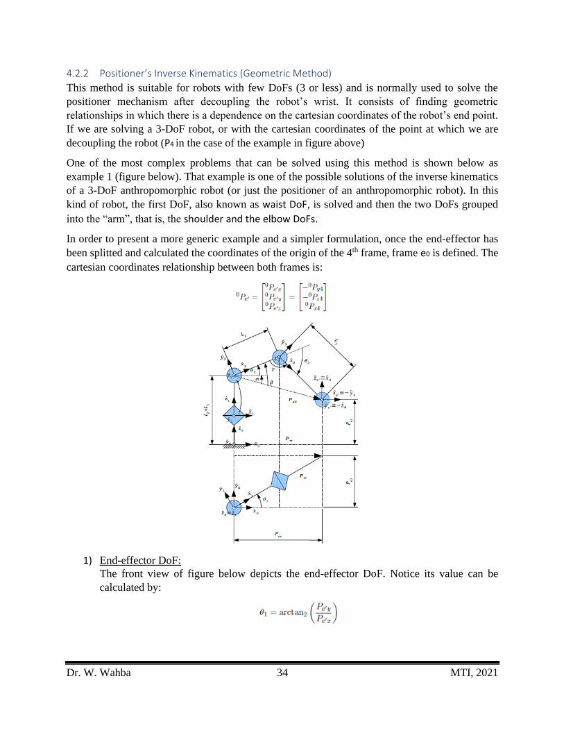
In order to present a more generic example and a simpler formulation, once the end-effector has

been splitted and calculated the coordinates of the origin of the 4th frame, frame e0 is defined. The

cartesian coordinates relationship between both frames is:

1) End-effector DoF: The front view of figure below depicts the end-effector DoF. Notice its value can be

calculated by:


Remember that Pe’x, Pe’y and Pe’z are the cartesian coordinates of the positioner mechanism’s

end-point Pe’7 and the function [arctan2] is the fourth-quadrant version of the arctan

function.

2) Shoulder and Elbow DoFs :

To solve the Shoulder (2) and Elbow (3) DoFs, we have to analyze the front view of

figure above.

Notice that the angles 2 and 3 can be expressed as below:

2 = - α 3 = -

Where α, and are auxiliary angles. Now let’s see how to calculate them. But first we

need to define a couple of auxiliary distances:

α is an angle defined by a right triangle in which the hypotenuse is Pe’R, the opposite leg is ||Pe’z -

(L0 + L1)|| and the adjacent leg is Pe’r. α can be obtained by the common trigonometric formula:

and are two of the angles of a triangle defined by L2, L3 and Pe’R distances. To calculate them

we have to apply the cosine theorem:

Notice that there is not an ambiguity of the quadrant to which α, and angles belong. Since they

are geometrical angles so they always belong to the first quadrant.

The solution we have just obtained is not the only valid solution of the inverse kinematics. It

corresponds to the hypothesis the robot in the configuration depicted in figure above. This solution

is called RIGHT-ARM & ELBOW-UP configuration.


Then we have to guess which are the remaining configurations, as well as the remaining solutions.

In this particular case, we can distinguish up to four configurations, next figure.

From analyzing this figure, it is easily proven that the general solution is:

4.2.3 Wrist’s Inverse Kinematics

In the case of the wrist mechanism, an analytical method is preferred to a geometrical one. This

method is based on the fact that the dot-product vectors depend on the cosines of the angle between

the above mentioned vectors. Since if we only calculate the cosines

we have an uncertainty about the quadrant angle, then we have to first calculate the cosines and

then the sinus for each DoF in the wrist.

The cosines angle is calculated using dot product between xi-1 and xi:

The sines angle should be calculated by the cross product. Since cross product formulae is more

complex than dot product, the recommended method is the calculation of the cosines (that is, dot

product) by means of the vectors define the complementary angle of i.


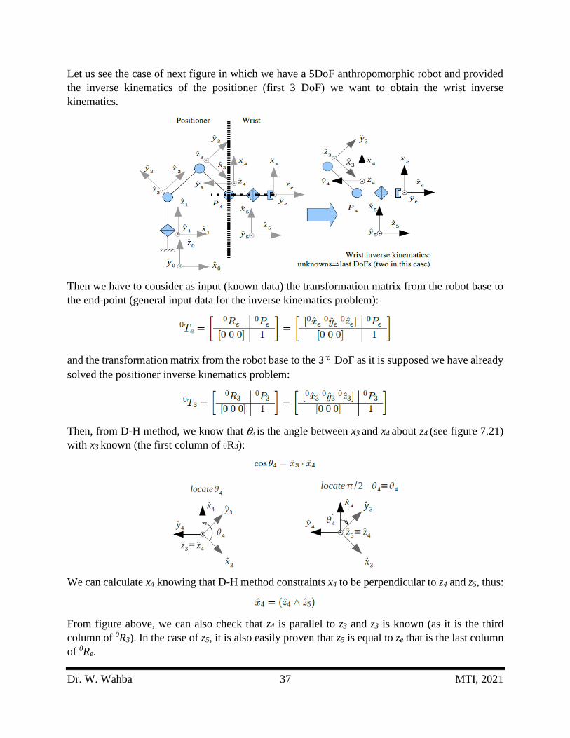
Let us see the case of next figure in which we have a 5DoF anthropomorphic robot and provided

the inverse kinematics of the positioner (first 3 DoF) we want to obtain the wrist inverse

kinematics.

Then we have to consider as input (known data) the transformation matrix from the robot base to

the end-point (general input data for the inverse kinematics problem):

and the transformation matrix from the robot base to the 3rd DoF as it is supposed we have already

solved the positioner inverse kinematics problem:

Then, from D-H method, we know that 4 is the angle between x3 and x4 about z4 (see figure 7.21)

with x3 known (the first column of 0R3):

We can calculate x4 knowing that D-H method constraints x4 to be perpendicular to z4 and z5, thus:

From figure above, we can also check that z4 is parallel to z3 and z3 is known (as it is the third

column of 0R3). In the case of z5, it is also easily proven that z5 is equal to ze that is the last column

of 0Re.


Then, last equation become:

We obtain the sin as the cos of the complementary angle:

Finally, we obtain the angle by means of arctan:

The last angle, 5 can be obtained following a similar procedure as the used for 4. But in this case,

we have:


Chapter 5

Jacobian Matrix

So far we have considered only the location (position and orientation) of the end-point, Pe, of the

robot with respect to the fixed base reference system and the joint position needed to achieve it.

Sometimes we also need to consider and to control the rate of change of the location of Pe, not just

its static location, to produce a constant speed straight line motion at Pe, for example.

We therefore need to know and to represent the relationship between the rates of change of the

individual joint values and the rate of change of location of Pe,

.

We call the matrix which represents this relationship the Jacobian Matrix, J, and this relationship

is between the joint value rates of change and the rate of change of the location of Pe, is shown

below.

This relationship can be expressed more formally as follows:

Forward Jacobian

Inverse Jacobian


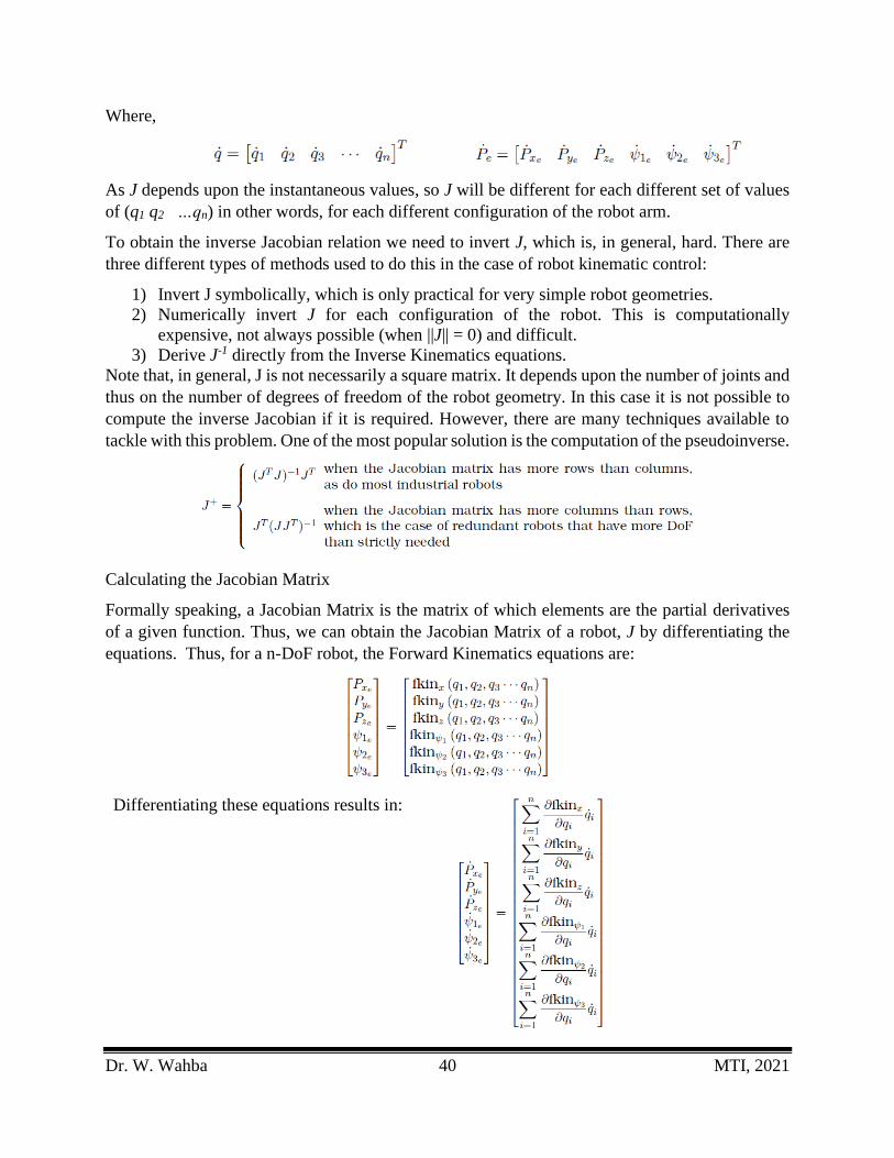
Where,

As J depends upon the instantaneous values, so J will be different for each different set of values

of (q1 q2 …qn) in other words, for each different configuration of the robot arm.

To obtain the inverse Jacobian relation we need to invert J, which is, in general, hard. There are

three different types of methods used to do this in the case of robot kinematic control:

1) Invert J symbolically, which is only practical for very simple robot geometries.

2) Numerically invert J for each configuration of the robot. This is computationally

expensive, not always possible (when ||J|| = 0) and difficult.

3) Derive J-1 directly from the Inverse Kinematics equations.

Note that, in general, J is not necessarily a square matrix. It depends upon the number of joints and

thus on the number of degrees of freedom of the robot geometry. In this case it is not possible to

compute the inverse Jacobian if it is required. However, there are many techniques available to

tackle with this problem. One of the most popular solution is the computation of the pseudoinverse.

Calculating the Jacobian Matrix

Formally speaking, a Jacobian Matrix is the matrix of which elements are the partial derivatives

of a given function. Thus, we can obtain the Jacobian Matrix of a robot, J by differentiating the

equations. Thus, for a n-DoF robot, the Forward Kinematics equations are:

Differentiating these equations results in:


Which can be written in matrix form as:

Which can be rewritten as:

where J* is the Jacobian Matrix. Notice that this Jacobian Matrix relates the temporal derivatives

of joint positions, that is, joint speeds with the temporal derivatives of end-point position.

However, the temporal derivatives of end-point position do not always represent the end-point

speed:

This equation illustrates the fact that the temporal derivative of position corresponds to a

translation speed, but neither the temporal derivative of Euler Angles nor of Quaternions

corresponds to an angular speed. However, it is possible to find a relationship between the temporal

derivatives of the representation of orientations and the angular speed. That relationship is verified

by pre-multiplying the temporal derivative vector by a matrix B. This matrix B is unique and its

expression depends on the used representation:

• In the case of Euler Angles:

For the Roll-Pitch-Yaw convention, the expression for B is:

• In the case of Rotation Axis- Rotation Angle representation:


Where:

&

Therefore, the Jacobian Matrix that relates Cartesian velocity with articular speed is:

5.1 Speed Propagation Method to Compute the Jacobian Matrix This method only presents real advantages for serial manipulators. It involves an iterative process

that starts with the hypothesis that the linear and angular speed at the base of the robot is known

(which is normally equal to zero because the robot is attached to a static surface). All joint speed

is computed from the base of the robot to the end-effector by the velocity propagation equations:

• angular speed propagation

• linear speed propagation

where iPi+1 is the vector that connects the origins of frames {i} and {i + 1}.

After finishing the iterative process, the Jacobian matrix is obtained as the matrix form of the last

given result (ee and ee). The summary of the whole process is shown in next flow chart.


5.2 Static of Robotic Manipulators If we consider a static robotic manipulator and we exert a force/torque on the endpoint, every robot

actuator should exert forces/torques to keep the robot stopped. The analysis of this problem

corresponds to the static analysis of the robot, or, rather the analysis of the forces/torque applied

to the robot that keeps the manipulator static.

From a mathematical point of view, the relationship between the applied force/torque on the end-

point of the robot and the forces/torque involved in the robot actuators to keep the manipulator

stopped are also given by the Jacobian Matrix of the manipulator:

Where: is the vector of force/torque applied by every actuator, and fe and ne are the force and

torque exerted on the end-point.

Notice that: the Jacobian Matrix given in this equation is the same as the Jacobian Matrix in

equation before. This equality is easily proven by the Virtual Work Theorem:

The Jacobian Matrix can also be calculated by performing a static equilibrium of the manipulator.

In the case of the serial manipulators, an iterative method called Force/Torque propagation can be

applied.

Force/Torque Propagation Method to Compute the Jacobian Matrix

As with the velocity propagation, this method only presents real advantages for serial

manipulators. It involves a iterative process that starts with the hypothesis that the force and torque

applied on the end-point is known (which is normally equal to a generic constant [fx fy fz nx ny nz]),

and then every torque/force exerted on each joint is computed from the end-point of the robot to

the 1st DoF (Notice that neither 0f0 nor 0n0 need to be calculated) by the force/torque propagation

equations:

After finishing the iterative process, the force/torque exerted on every joint is obtained using the

following equations:


In other words, the above equations imply the extraction of the fz value (if the DoF is prismatic) or

nz (if the DoF is rotational). After obtaining 1 … n, the Jacobian matrix is obtained as the matrix

form of the equations for 1 …. n. The summary of the whole process is shown in next flow chart.

5.3 Singularities and Singular Configurations If, for any particular configuration of the robot arm that is in movement, the motion performance

of a robot can be degraded abruptly, that configuration is a singular configuration. In those

configurations, the Jacobian Matrix loses range and in the case of square Jacobian Matrices they

become singular.

We can measure how far the manipulator is from a singular configuration thanks to the following

manipulability index

In the case of square matrices, that index becomes the determinant:


In a singular configuration, the manipulability index becomes zero:

For a singular configuration, J-1 does not exist, it is not mathematically defined when ||J|| = 0, so,

as a result, the relation between articular speed (q ) and the cartesian speed (Ve) is not defined.

Consequently, neither is the relationship between articular force/torque (q ) and cartesian

force/torque (f & n).

Singular configuration occurs when two or more joint axes become aligned in space. When this

happens, the serial robot geometry effectively loses one (or more) independent degrees of freedom:

two or more of the degrees of freedom become mutually dependent (the case of parallel robotics,

the geometry gains one (or more) degrees of freedom and losses stiffness).

When that-configurations near to a singular configuration, the elements of J-1 can have very large

values. This means that, for even small values of Ve there will be large values in q., which will

most likely be too large for the joint motors to actually generate.

The loss of one or more effective degrees of freedom thus occurs not just at a singular

configuration, but also in a region (a volume in joint space) around it.

According to Craig, singular configurations are classified into two different kinds:

1) Workspace Boundary Singularities, which occur when the robot manipulator is fully

extended or folded onto itself so that Pe is at or near the boundary of the robot workspace.

In such configurations, one or more joints will be at their limits of range of movement, so

that they will not be able to maintain any movement at any given speed. This effectively

makes J a singular matrix.

2) Workspace Interior Singularities, which occur inside the robot workspace away from any

of the boundaries and are generally caused by two or more joint axes become aligned.

Three different courses of action can be taken to avoid singular configurations:

1) Increase robot manipulator’s degrees of freedom, perhaps by attaching a tool or gripper to

Pe, which has one or two degrees of freedom itself.

2) Restrict the movements that the robot can be programmed to make so as to avoid any

singular configurations.

3) Dynamically modify J to remove the offending terms, and thus return ||J|| 6= 0. This means

identifying the column and row of J that need to be removed.


Chapter 6

References

1) J.J. Craig. INTRODUCTION TO ROBOTICS, MECHANICS AND CONTROL. Addison

Wesley, 1986.

2) J. Critchlow. INTRODUCTION TO ROBOTICS. Macmillan Publishing Co, 1985.

3) Ashitava Ghosal. ROBOTICS Fundamental Concepts and Analysis. Oxford University

Press, 2006.

4) P. Mckerrow. INTRODUCTION TO ROBOTICS. Addison-Wesley Longman Publishing

Co., Inc., Boston, MA, USA, 1991.

5) R. P. Paul. ROBOT MANIPULATORS: MATHEMATICS, PROGRAMMING AND

CONTROL. Addison Wesley, 1981.

6) L. Sciavicco and B. Siciliano. MODELLING AND CONTROL OF ROBOT

MANIPULATORS. Springer, 2000.

Documents

Lectures Notes of Robot Technology