Embed Size (px)
Citation preview
Lectures on Complex Analysis
M. Pollicott

Contents
1. Introduction 51.1. A little history 51.2. Notation 61.3. Some useful reference books 72. A few basic ideas 72.1. The Riemann sphere 72.2. Mobius maps 92.3. Two applications 122.4. Classification of Mobius maps and their behaviour 152.5. cross-ratios of quadruples of complex numbers 182.6. Problems 203. Analyticity 213.1. Ingredients for the first definition (using power series) 223.2. Ingredients for the second definition (using complex differentiability) 223.3. Ingredients for the third definition (using the Cauchy-Riemann
Equations) 234. Definitions of analyticity 244.1. The main result 245. Integrals and Cauchy’s Theorem 285.1. Integration on piecewise continuous curves 285.2. parameterization of the curve of integration 285.3. Theorems of Gousart and Cauchy 325.4. Immediate applications of Cauchy’s Theorem 365.5. Converse to Cauchy’s Theorem 385.6. Problems 396. Properties of analytic functions 406.1. Logarithms and roots 406.2. Location of zeros: Argument Principle and Rouche’s Theorem 416.3. Liouville’s Theorem and the Fundamental Theorem of Algebra 456.4. Identity Theorem 466.5. Families of functions and Montel’s Theorem 476.6. Problems 496.7. More problems 507. Riemann Mapping Theorem 517.1. Riemann Mapping Theorem 517.2. Christoffel-Schwarz Theorem 537.3. examples 577.4. Generalizations of the Schwarz-Christofel theorem 607.5. Application: Fluid dynamics 607.6. Problems 607.7. More problems 628. Behaviour of analytic functions 628.1. The Maximum Modulus Principle 638.2. The Schwarz Lemma 63
3
4 CONTENTS
8.3. Pick’s lemma 649. Harmonic functions 659.1. Harmonic conjugates 669.2. Poisson Integral formula 679.3. Mean Value Property and Maximum Principle for harmonic functions 719.4. Schwarz reflection principle for harmonic functions 729.5. Application: Continuous extensions to the boundary of analytic
bijections 739.6. Problems 7410. Singularities 7510.1. Removable singularities 7510.2. Analogues of Cauchy’s theorem 7610.3. Laurent’s Theorem 7710.4. Classification of singularities 8010.5. Behaviour at singularities 8011. Entire functions, their order and their zeros 8211.1. Growth of entire functions 8211.2. Factorization of entire functions 8412. Prime number theorem 8612.1. Riemann zeta function 8612.2. A related complex function 8712.3. A related counting function 8712.4. Finiteness of integrals 8812.5. Proof of the Prime Number Theorem 9013. Further Topics 9113.1. Weierstrass’s elliptic function 9213.2. Picard’s Little theorem 9213.3. Runge’s theorem 9213.4. Conformality: Property of analytic maps 9213.5. Functions of several complex variables 93
1. INTRODUCTION 5
1. Introduction
Complex analysis is one of the classical branches in mathematics with rootsin the 19th century and just prior. Complex analysis, in particular the theory ofconformal mappings, has many physical applications and is also used throughoutanalytic number theory. In modern times, it has become very popular through anew boost from complex dynamics and the pictures of fractals produced by iteratingholomorphic functions. Another important application of complex analysis is instring theory which studies conformal invariants in quantum field theory.
1.1. A little history. The study complex numbers arose from try to findsolutions to polynomial equations. Al-Khwarizmi (780-850) in his book Algebrahad solutions to quadratic equations of various types. Under the caliph Al-Mamun(reigned 813-833) Al-Khwarizmi became a member of the House of Wisdom inBagdad,
The first to solve the polynomial equation x3 + px = q was Scipione delFerro (1465-1526). On his deathbed, del Ferro confided the formula to his pupilAntonio Maria Fiore, who subsequently challenged another mathematician Nicola“Tartaglia” Fontana (1500-1557) to a mathematical contest on solving cubics. (Thename Tartaglia means “stammerer” a symptom of injuries acquired aged 12 dur-ing the french attack on his home town of Bresca). The night before the contest,Tartaglia rediscovered the formula and won the contest. Tartaglia in turn told theformula (but not the proof) to an influential mathematician Gerolamo Cardano(1501-1576), provided he signed an oath to secrecy. However, from a knowledge ofthe formula, Cardano was able to reconstruct the proof. Later, Cardano learnedthat del Ferro, not Tartaglia, had originally solved the problem and then, feelingunder no further obligation towards Tartaglia, proceeded to publish the result inhis Ars Magna (1545). Cardano was also the first to introduce complex numbersa +√b into algebra, but had misgivings about it. In the Ars magna he observed,
for example, that the problem of finding two numbers that add to 10 and multiplyto 40 was satisfied by 5 +
√−15 and 5 −
√−15 but regarded the solution as both
absurd and useless. Cardan was also said to have correctly predicted the exact dateof his own death (but it has also been claimed that he achieved this by committingsuicide!).
Rene Descartes (1596-1650), the mathematician and philospher coined the termimaginary: “For any equation one can imagine as many roots [as its degree wouldsuggest], but in many cases no quantity exists which corresponds to what one imag-ines.”
Abraham de Moivre (1667-1754), a protestant, left France to seek religiousrefuge in London at eighteen years of age. There he befriended Isaac Newton. In1698 he mentions that Newton knew, as early as 1676 of an equivalent expressionto what is today known as de Moivres theorem (and is probably one of the bestknown formulae) which states that:
(cos(θ) + i sin(θ))n = cos(nθ) + i sin(nθ)
where n is an integer. (De Moivre, like Cardan, is famed for predicting the day ofhis own death. He found that he was sleeping 15 minutes longer each night andsumming the arithmetic progression, calculated that he would die on the day thathe slept for 24 hours.)
Leonhard Euler (1707-1783) introduced the notation i =√−1 in his book
Introductio in analysin innitorum in 1748, and visualized complex numbers as pointswith rectangular coordinates, but did not give a satisfactory foundation for complexnumbers. In contrast, there are indications that Carl Friedrich Gauss (1777-1855).had been in possession of the geometric representation of complex numbers since
6 CONTENTS
1796, but it went unpublished until 1831, when he submitted his ideas to the RoyalSociety of Gottingen. It was Gauss who introduced the term complex number.
Joseph-Louis Lagrange (1736-1813) showed that a function is analytic if it hasa power-series expansion However, it is Augustin-Louis Cauchy (1789-1857) who re-ally initiated the modern theory of complex functions in an 1814 memoir submittedto the French Academie des Sciences.
Although the term analytic function was not mentioned in his memoir, the con-cept is present there. The memoir was eventually published in 1825. In particular,contour integrals appear in this memoir (although Poisson had written a 1820 pa-per with a path not on the real line). Cauchy also gave proofs of the FundamentalTheorem of Algebra (1799, 1815) which, as we will see, has analytic proof . Insummary, Cauchy, gave the foundation for most of the modern ideas in the field,including:
(1) integration along paths and contours (1814);(2) calculus of residues (1826);(3) integration formulae (1831);(4) Power series expansions (1831); and(5) applications to evaluation of denite integrals of real functions
The Cauchy- Riemann equations (actually dating back to dAlembert 1752, thenEuler 1757, dAlembert 1761, Euler 1775, Lagrange 1781) are also usually attributedto Cauchy 1814-1831 and Riemann 1851.
Cauchy resigned from his academic positions in France in 1830 rather than toswear an oath of allegence to the new government. However, he felt able to resumehis career in France in 1848, when the oath was finally abolshed.
Regarding subsequent work, Karl Weierstrauss (1815-1897) formulated analyt-icity in terms of existence of a complex derivative, which is the perspective takenin most textbooks, and Georg Riemann (1826-1866) made fundamental use of thenotion of conformality (previously studied by Euler and Gauss). Later contribu-tions were made by Poincare to conformal maps and Teichmuller to quaai-conformalmaps.
1.2. Notation. We denote by C the complex numbers. If z ∈ C then we canwrite z = x + iy where x, y ∈ R. We denote the real and imaginary parts byx = Re(z) and y = Im(z). We then write the absolute value as |z| =
√x2 + y2.
Occasionally it is useful to write complex numbers in radial coordinates, i.e.,z = reiθ where r > 0 and 0 ≤ θ < 2π.
We denote by z = x − iy = re−iθ the complex conjugate. If z, w ∈ C then wewrite
[z, w] = αz + (1− α)w : 0 ≤ α ≤ 1
for the line segment joining them.

2. A FEW BASIC IDEAS 7
Exercise 1.1. Show that the map φ : C→M2(R) (= 2× 2 real matrices)
φ : x+ iy 7→(x y−y x
).
is a monomorphism.
1.3. Some useful reference books.
(1) R. Churchill and J. Brown, Complex Variables and Applications (ISBN0-07-010905-2). This is a fairly readable account including much of thematerial in the course.
(2) I. Stewart and D. Tall, Complex Analysis (ISBN 0-52-128763-4). This isa popular and accessible book.
(3) L. Alhfors, Complex Analysis: an Introduction to the Theory of AnalyticFunctions of One Complex Variable (ISBN 0-07-000657-1). This is a classictextbook, which contains much more material than included in the courseand the treatment is fairly advanced.
(4) S. Krantz and R. Greene, Function Theory of One Complex Variable(ISBN 0-82-183962-4). This is a nice textbook, which contains much morematerial than included in the course.
(5) S. Krantz, Complex Analysis: The Geometric Viewpoint (0-88-385035-4).The first chapter gives a nice summary of some of the ideas in the course.The rest of the book is very interesting, but too geometric for this course.
2. A few basic ideas
2.1. The Riemann sphere. It is convenient to add an extra point to C. Inorder to accommodate the extra point ∞, we need to extend the complex plane byadding this point in to get the Riemann sphere.
We denote by C = C ∪ ∞ the Riemann sphere. There is a natural “stereo-graphic” projection between the sphere (minus the “north pole” (1, 0, 0)) and thecomplex plane
π : (x1, x2, x3) ∈ R3 : x2 + x22 + x2
3 = 1 − (1, 0, 0) → C
defined by
π(x1, x2, x3) = z :=(
x1
1− x3
)+i(
x2
1− x3
).
In particular, 0 it the image of the south pole (0, 0,−1), and the unit circle |z| = 1is the image of the equator x3 = 0.
Definition 2.1. A circle on the sphere corresponds to the intersection of x21 +
x22 + x2
3 = 1 with a plane ax+ by + cz = d.

8 CONTENTS
The following is easy to prove.
Lemma 2.2. The stereographic projection of a circle on the sphere is either acircle or a line in C.
Proof. The image of the intersection under the projection can be written as
a(z + z)− ib(z − z) + c(|z|2 − 1) = d(|z|2 + 1)
If we write z = x+ iy then
(d− c)(x2 + y2)− 2ax− 2by + (d+ c) = 0.
Case I: If c = d then this is the equation of a straight line.
Case II: If c 6= d then
x2 + y2 − 2axd− c
− 2byd− c
+(d+ c)d− c
= 0
which we can rearrange as(x− a
d− c
)2
+(y − b
d− c
)2
=a2 + b2 + (c2 − d2)
(d− c)2.
It only remains to show that a2 + b2 + c2 − d2 > 0 to see this is the equation of acircle. However,
|α0| = |ax+ by + cz| ≤√x2 + y2 + z2︸ ︷︷ ︸
=1
√a2 + b2 + c2
by the usual Cauchy-Schrwartz inequality and we are done.
Note that in the proof there is an equality in the last line only when (a, b, c) =λ(x1, x2, x3) for some λ, i.e., the plane is tangent to the sphere.
Remark 2.3. The inverse images of a points z ∈ C is a triple (x1, x2, x3) lyingon the sphere and satisfying |z|2 = (x2
1 + x22)/(1 − x3)2 = (1 + x3)/(1 − x3) (since
x21 + x2
2 + x23 = 1). We can then write
x1 =z + z
1 + |z2|since 1− x3 =
2|z|2 + 1|
.
Similarly,
x2 =z − z
1 + |z2|and x3 =
|z|2 − 11 + |z2|
.
We deduce that
(x1, x2, x3) =(
z + z
1 + |z2|,z − z
1 + |z2|,|z|2 − 11 + |z2|
).
This completes the proof.
Exercise 2.4. Prove the converse, i.e., the preimage of a circle or a straightline in C is a circle on the Riemann sphere.

2. A FEW BASIC IDEAS 9
Remark 2.5. To associate the appropriate topology to C we take the usualopen sets in C plus the complements of compact sets union with the point ∞. Thismeans that we can interpret zn → z in the usual sense if z 6= ∞. However, we saythat zn → +∞ if for every K > 0 we have there exists N > 0 such that |z| > K.Then C is homeomorphic to the ball minus the ”north pole”. The approrpiatemetric for C comes form the standard metric on the ball, i.e.,
d((x1, x2, x3), ((x′1, x′2, x′3)) =
√(x1 − x′1)2 + (x2 − x′2)2 + (x3 − x′3)2
=√
2(1− x1x′1 + x2x′2 + x3x′3).
If z := π((x1, x2, x3)) and w := π((x′1, x′2, x′3)) then we can define a natural metric
on C ∪ ∞ by
d(z, w) = d((x1, x2, x3), ((x′1, x′2, x′3)) =
|z − w|√(1 + |z|2)(1 + |w|2)
where (x1, x2, x3), (x′1, x′2, x′3) 6= (0, 0, 1) (i.e., z, w 6=∞) and
d(z,∞) := d((x1, x2, x3), (0, 0, 1)) =2√
1 + |z|2.
Exercise 2.6. Check all the above formulae.
2.2. Mobius maps. We can consider a, b, c, d ∈ C with ad 6= bc,.
Definition 2.7. We define a map f : C − −dc → C by f(z) = az+bcz+d . (If
ad = bc then f(C) = ∞, a single point).
Remark 2.8. We can also assume without loss of generality that ad− bc = 1,since we see that replacing a, b, c, d to λa, λb, λc, λd gives the same map. We willadopt this convention when convenient.
Observe that if c = 0 then f(∞) = ∞, i.e., ∞ is a fixed point. On the otherhand, if c 6= 0 then letting z 7→ −d/c we see that f(−d/c) = ∞. Letting z → +∞we can write that f(∞) = a/c.
Lemma 2.9. If c 6= 0 then the Mobius map f is invertible, and its inverse isalso a Mobius map (and thus f : C→ C is a homeomorphism).
Proof. If f(z) = az+bcz+d with ad − bc = 1 then we can define f−1(z) = dz−b
−cz+a .We can then explicitly check f f−1(z) = z and f−1 f(z) = z. For example,
f(f−1(z)) =a(dz−b−cz+a
)+ b
c(dz−b−cz+a
)+ d
=a (dz − b) + b (−cz + a)c (dz − b) + d (−cz + a)
=(ad− bc) z(ad− bc)
= z
Lemma 2.10. If f1 and f2 are Mobius maps then so is the composition f1 f2
Proof. This follows immediately by substitution. (Exercise)
In particular, the set of Mobius maps forms a group.
10 CONTENTS
Example 2.11. There are four fundamental examples of Mobius transforma-tions f : C→ C.
a) Translations: z 7→ z + b = 1.z+b0.z+1 where b ∈ C. These are often called
parabolic transformations.b) Rotations: z 7→ az =
√a.z+0
0.z+√a−1 where |a| = 1. These are often called
elliptic transformations.c) Expansions (and Contractions): z 7→ λz =
√λ.z+0
0.z+√λ−1 with λ > 1 (or
0 < λ < 1) and λ real. These are often called hyperbolic transformations.d) Inversions: z 7→ 1
z .
We can use this to deduce the following.
Lemma 2.12. Every Mobius map can be written as a composition of Mobiusmaps of the above type.
Proof. Every Mobius map is a combination of three types of maps f(z) = Az,f(z) = z +B and f(z) = 1/z, where A,B ∈ C, since we can write
az + b
cz + d=
ac (cz + d) +
(b− ad
c
)cz + d
=a
c+
(b− ad
c
)cz + d
which is a composition of there
z 7→ cz 7→ cz + d 7→ 1cz + d
7→(b− ad
c
)(1
cz + d
)7→(b− ad
c
)(1
cz + d
)+a
c
The follow result is very useful. Consider circles in the complex plane of theform C := z ∈ C : |z − z0| = r where z0 ∈ C and r > 0.
Theorem 2.13. The image of a circle or straight line under a Mobius trans-formation is a circle or straight line.
Proof. It suffices to consider three different types of Mobius transfomations:
(1) If f(z) = Az where A ∈ C with A 6= 0 then the image f(C) is a circle.(2) If f(z) = z +B where B ∈ C then the image f(C) is a circle.(3) If f(z) = 1/z then the image f(C) is a circle. We first observe if z = x+iy
lies on a circle centred at z0 = x0 + iy0 of radius r > 0 then
(x− x0)2 + (y − y0)2 = r2 (1)
Consider the set of z such that
|z − p||z − q|
= k (2)
where p, q ∈ C and k > 0. If p = u+ iv and q = s+ it then this becomes:
(x− u)2 + (y − v)2 = k2((x− s)2 + (y − t)2
)(3)
In particular, we can rewrite (1) in terms of (3) by choosing p, q, k suchthat
x0 =(u− k2s)
1− k2
y0 =v − k2t
1− k2
r2 = −u2 + v2 − k2(s2 + t2)
1− k2+(u− sk2
1− k2
)+(v − tk2
1− k2
)> 0.

2. A FEW BASIC IDEAS 11
Finally we can see that if z satisfies (2) then
|z − p||z − q|
= k ⇐⇒
∣∣∣ 1z − 1p
∣∣∣∣∣∣ 1z − 1q
∣∣∣ =q
pk (4)
i.e., a version of (3) (with p replaced by 1p , q replaced by 1
q and k replacedby q
pk). In particlar, the image of the circle given by (2) is a circle givenby (3).
Theorem 2.14. For distinct z1, z2, z3 ∈ C and distinct w1, w2, w3 ∈ C thereexists a unique Mobius map f : C→ C such that f(zi) = wi, for i = 1, 2, 3.
Proof. We first prove existence and then uniqueness.
Existence. Consider the case that z1, z2, z3 6=∞. Let
S(z) =(z − z2)(z1 − z3)(z − z3)(z1 − z2)
then we see that S(z1) = 1, S(z2) = 0, S(z3) =∞. Consider
T (z) =(z − w2)(z1 − w3)(z − w3)(z1 − w2)
then we see that T (w1) = 1, T (w2) = 0, T (w3) =∞. If we define f(z) := S−1T (z)then we can then observe that f(zi) := T−1 S(zi) = wi (i = 1, 2, 3).
In the case that z1 =∞ then we let S(z) = z−z2z−z3 and similarly for T .
In the case that z2 =∞ then we let S(z) = z1−z3z−z3 and similarly for T .
In the case that z3 =∞ then we let S(z) = z−z2z1−z2 and similarly for T .
Uniqueness. We can assume without loss of generality that w1 = 1, w2 = 0, w3 =∞. (Otherwise we can additionally compose with a Mobius map g; C → C takingw1, w2, w3 to 1, 0,∞, respectively, and then we can apply the following argumentto show that f1 g−1 = f2 g−1, which therefore gives us f1 = f2). Assume thatfj : C → C are two Mobius maps j = 1, 2 such that fj(1) = z1, fj(0) = z2,fj(∞) = z3. Since S(z) = f−1
1 f2(z) is a Mobius transformation we can write
S(z) =az + b
cz + d
Moreover, f−11 f2 : C→ C fixes the three points 1, 0,∞. In particular, we see that
S(0) = b/d = 0 =⇒ b = 0
S(∞) = a/c =∞ =⇒ c = 0, and
S(1) = (a+ b)/(c+ d) = a/d = 1
from which we deduce that S(z) = z for all z, i.e., f1 = f2.
Let us consider a could of examples of this result.
Example 2.15. Find the Mobius transformation f which maps −1, 0, 1 to thepoints −i, 1, i.
Assume that f(z) = az+bcz+d . Since f(0) = b
d = 1 we have b = d and f(z) = az+bcz+b .
Similarly, since f(−1) = −ia+b−ic+b = 1 =⇒ ic− ib = −a+ b and f(1) = ia+b
ic+b = i =⇒ic+ ib = a+ b. Adding the last two equations gives c = −ib and subtracting givesa = ib. Thus
f(z) =ibz + b
−ibz + b=
iz + 1−iz + 1
=i− zi+ z
.
(Formally, we should also multiply the coefficients by constant to get ad− bc = 1)
12 CONTENTS
Example 2.16. Let D = z ∈ C : |z| < 1 be the open unit disk unit and letH = z ∈ C : Im(z) > 0 be the upper half-plane. Find a surjective Mobius mapf : H→ D.
Actually, the map in the previous example works (as one might guess from thethree points in the boundary of H being mapped to three points in the boundaryof D). To see this, let z = x+ iy with y > 0 then
|f(z)| =∣∣∣∣ i− (x+ iy)i+ (x+ iy)
∣∣∣∣2 =∣∣∣∣−x+ i(1− y))x+ i(y + 1)
∣∣∣∣2 =x2 + (1− y)2
x2 + (1 + y)2< 1,
i.e., f(z) ∈ D.
Example 2.17. Fix a ∈ C and then we can define a Mobius map f :C → C by
f(z) =a− z1− az
Notice that
|f(z)|2 =|a− z|2
|a− az|2=|a|2 − 2Re(az) + |z|2
1− 2Re(az) + |az|2
It is easy to check that if |z| = 1 if and only if |f(z)| = 1. Moreover, if |f(z)| < 1 isequivalent to
|a|2 + |z|2 < 1 + |az|2 < 1 ⇐⇒ (1− |a|2)(1− |z|2) > 0 ⇐⇒ |z| < 1
since |a| < 1. We can conclude that f : D→ D.
2.3. Two applications.
Application 2.18 (Apollonion Circle Packings). This is related to taking threecircles in the plane.
Theorem 2.19 (Apollonius). Given three mutually tangent circles C1, C2, C3
there are precisely two circles C, C ′ tangent to all three.
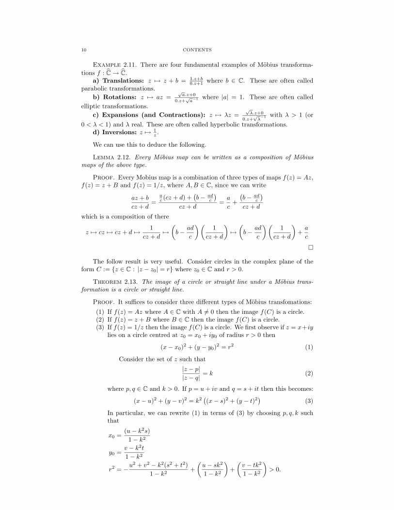
Proof. We can write this in a number of steps.
Step 1: Let ξ be the point of intersection C1 ∩ C2 of two of the circles. We canapply the Mobius transformation f(z) = 1
z−ξ then f(ξ) = ∞ and C1 − ξ andC2 − ξ are mapped to disjoint (and thus parallel) straight lines L1 and L2.
Since C1 and C3 are tangent at one point η, say, and C2 and C3 are tangent atone point ρ, say, then the image C4 = f(C3) is another circle tangent to L1 and L2.
2. A FEW BASIC IDEAS 13
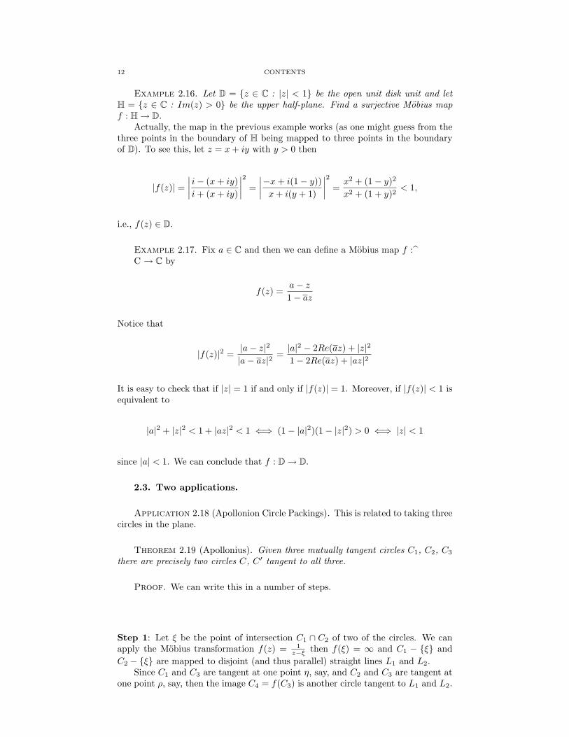
Step 2: We can trivially translate C4 between the two parallel lines L1, L2 toprecisely two more circles C5 and C6 of the same radius such that: C5 and C6 areboth tangent to both L1 and L2 and C3.
Step 3: We then define C = f−1(C5) and C ′ = f−1(C6). Since again Mobiustransformations take circles to circles (where straight lines are understood as circlespassing through infinity) we deduce that C,C ′ are the only two such circles tangentto C1, C2, C3.
Theorem 2.20. Descartes Theorem: Given four mutually tangent circles C1,C2, C3 and C4 whose radii are r1, r2, r3, r4 then F (r1, r2, r3, r4) = 0 where
F (r1, r2, r3, r4) = 2(r−21 + r−2
2 + r−23 + r−2
4 )− (r−11 + r−1
2 + r−13 + r−1
4 )2 (1)
Proof. We begin with two simple estimates. Consider a circle E of radius k.
(1) We can reflect in it a second circle C of radius r whose centres are separatedby d > r + k. In particular, the circles are disjoint and have disjointinteriors. The image circle f(E′) with have radius k2r/(d2 − r2).
(2) Consider next a straight line L at a distance b > k from the centre of E.We can reflect it in the circle E and the image is a circle of radius k2/2b.
14 CONTENTS
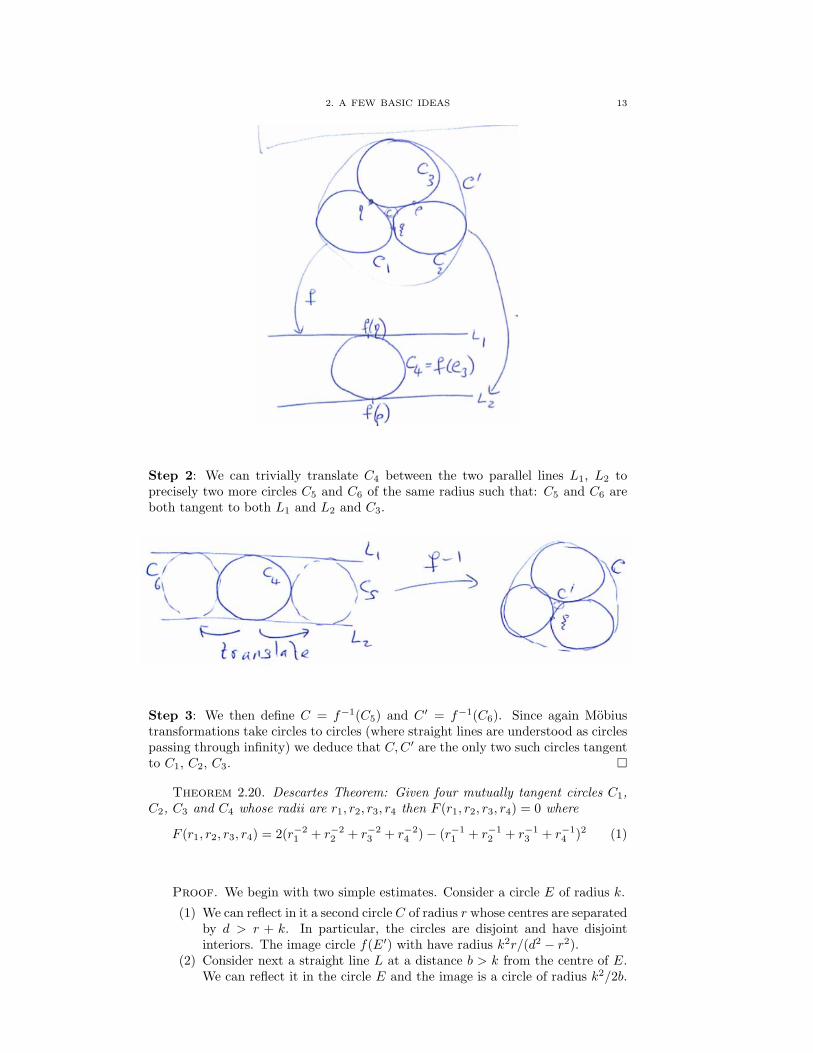
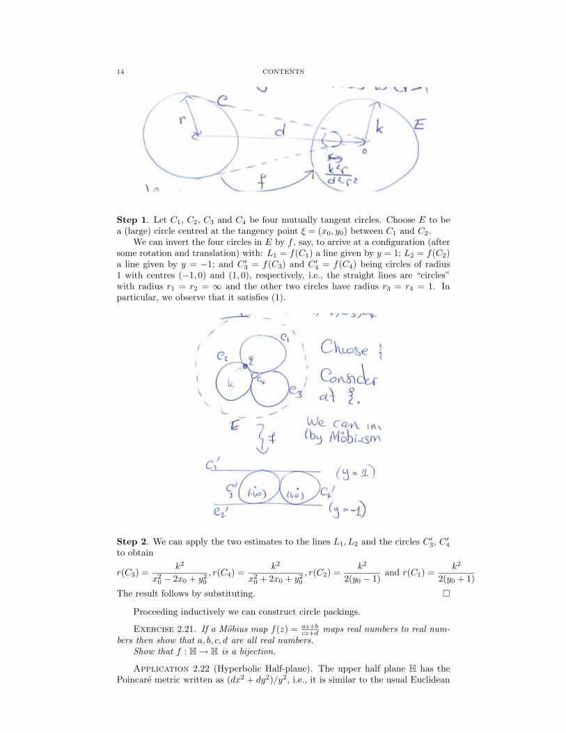
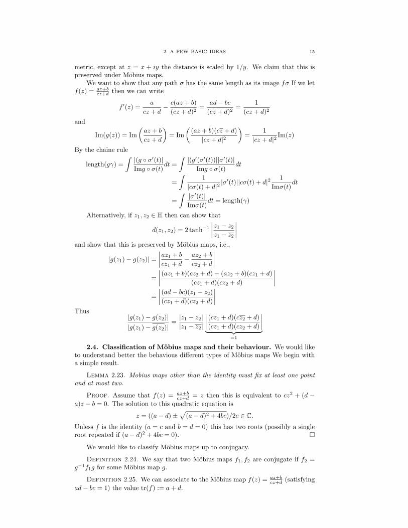
Step 1. Let C1, C2, C3 and C4 be four mutually tangent circles. Choose E to bea (large) circle centred at the tangency point ξ = (x0, y0) between C1 and C2.
We can invert the four circles in E by f , say, to arrive at a configuration (aftersome rotation and translation) with: L1 = f(C1) a line given by y = 1; L2 = f(C2)a line given by y = −1; and C ′3 = f(C3) and C ′4 = f(C4) being circles of radius1 with centres (−1, 0) and (1, 0), respectively, i.e., the straight lines are “circles”with radius r1 = r2 = ∞ and the other two circles have radius r3 = r4 = 1. Inparticular, we observe that it satisfies (1).
Step 2. We can apply the two estimates to the lines L1, L2 and the circles C ′3, C ′4to obtain
r(C3) =k2
x20 − 2x0 + y2
0
, r(C4) =k2
x20 + 2x0 + y2
0
, r(C2) =k2
2(y0 − 1)and r(C1) =
k2
2(y0 + 1)
The result follows by substituting.
Proceeding inductively we can construct circle packings.
Exercise 2.21. If a Mobius map f(z) = az+bcz+d maps real numbers to real num-
bers then show that a, b, c, d are all real numbers.Show that f : H→ H is a bijection.
Application 2.22 (Hyperbolic Half-plane). The upper half plane H has thePoincare metric written as (dx2 + dy2)/y2, i.e., it is similar to the usual Euclidean
2. A FEW BASIC IDEAS 15
metric, except at z = x + iy the distance is scaled by 1/y. We claim that this ispreserved under Mobius maps.
We want to show that any path σ has the same length as its image fσ If we letf(z) = az+b
cz+d then we can write
f ′(z) =a
cz + d− c(az + b)
(cz + d)2=
ad− bc(cz + d)2
=1
(cz + d)2
and
Im(g(z)) = Im(az + b
cz + d
)= Im
((az + b)(cz + d)|cz + d|2
)=
1|cz + d|2
Im(z)
By the chaine rule
length(gγ) =∫|(g σ′(t)|Img σ(t)
dt =∫|(g′(σ′(t))||σ′(t)|
Img σ(t)dt
=∫
1|cσ(t) + d|2
|σ′(t)||cσ(t) + d|2 1Imσ(t)
dt
=∫|σ′(t)|Imσ(t)
dt = length(γ)
Alternatively, if z1, z2 ∈ H then can show that
d(z1, z2) = 2 tanh−1
∣∣∣∣z1 − z2
z1 − z2
∣∣∣∣and show that this is preserved by Mobius maps, i.e.,
|g(z1)− g(z2)| =∣∣∣∣az1 + b
cz1 + d− az2 + b
cz2 + d
∣∣∣∣=∣∣∣∣ (az1 + b)(cz2 + d)− (az2 + b)(cz1 + d)
(cz1 + d)(cz2 + d)
∣∣∣∣=∣∣∣∣ (ad− bc)(z1 − z2)(cz1 + d)(cz2 + d)
∣∣∣∣Thus
|g(z1)− g(z2)||g(z1)− g(z2)|
=|z1 − z2||z1 − z2|
∣∣∣∣ (cz1 + d)(cz2 + d)(cz1 + d)(cz2 + d)
∣∣∣∣︸ ︷︷ ︸=1
2.4. Classification of Mobius maps and their behaviour. We would liketo understand better the behavious different types of Mobius maps We begin witha simple result.
Lemma 2.23. Mobius maps other than the identity must fix at least one pointand at most two.
Proof. Assume that f(z) = az+bcz+d = z then this is equivalent to cz2 + (d −
a)z − b = 0. The solution to this quadratic equation is
z = ((a− d)±√
(a− d)2 + 4bc)/2c ∈ C.Unless f is the identity (a = c and b = d = 0) this has two roots (possibly a singleroot repeated if (a− d)2 + 4bc = 0).
We would like to classify Mobius maps up to conjugacy.
Definition 2.24. We say that two Mobius maps f1, f2 are conjugate if f2 =g−1f1g for some Mobius map g.
Definition 2.25. We can associate to the Mobius map f(z) = az+bcz+d (satisfying
ad− bc = 1) the value tr(f) := a+ d.
16 CONTENTS
Lemma 2.26. The value tr(f) is preserved by conjugacy, i.e., if f1, f2 are con-jugate then tr(f1) = tr(f2)
Proof. Since every Mobius map g can be written as a composition of basicMobius transformations (translation, inversion and rotation) it suffices to show theresult where g is of each type.Translations: if g(z) = z + β then we can explicitly write
f2(z) = g−1f1g(z) =a(z − β) + b
c(z − β) + d+ β
=a(z − β) + b+ β(c(z − β) + d))
c(z − β) + d
=z(a+ βc) + (b+ βd− βa− β2c)
cz + (d− βc)
and we see that tr(f2) = (a+ βc) + (d− βc) = a+ d = tr(f1).Inversions: If g(z) = 1/z then
f2(z) = g−1f1g(z) =a/z + b
c/z + d
=a+ bz
c+ dz
and we see that tr(f2) = d+ a = tr(f1).Rotations: If g(z) = αz then
f2(z) = g−1f1g(z) =1α
(aαz + b
cαz + d
)=az + b/α
cαz + d
and we see that tr(f2) = a+ d = tr(f1).
Definition 2.27. We say that a rational map is parabolic it it has preciselyone fixed point in C
In particular, being parabolic is easily seen to be a conjugacy invariant (i.e.,if f1 has a single fixed point z0, say, then f2 has a single fixed point g−1z0. Inparticular, if f1 has a fixed point f1(z0) = z0 we can choose g so that g(∞) = z0
and then the conjugate map f := f2 fixes ∞.
Lemma 2.28. Let f be a Mobius map with f(∞) =∞.(1) Then f is of the form f(z) = αz + β;(2) f has a second distinct fixed point (i.e., it is not parabolic) if and only if
α 6= 1;(3) if the second fixed point is 0 (i.e., f(0) = 0) then f(z) = αz.
Proof. (1) Since f(∞) = ∞ this immediately implies that f2(z) = αz + β, forsome α, β ∈ C.(2) If f has a second point z0, say, (other than ∞) then f(z0) = αz0 + β = z0, i.e,z0 = β
α−1 with α 6= 1. In particular, if α 6= 1 then f has a second fixed point (inaddition to ∞). Conversely, if α = 1 then f has no other fixed points except ∞since f(z) = z + β is a straightforward translation. (In the degenerate case β = 0this is just the identity.)(3) Since f(0) = 0 we see that β = 0 and the result follows.

2. A FEW BASIC IDEAS 17
Remark 2.29. In fact Mobius transformations f1, f2 are conjugate if and onlyif tr(f1)2 = tr(f2)2
The non-identity Mobius transformations are commonly classified into threetypes:
(1) parabolic (conjugate to z 7→ z + β with a single fixed point ∞);(2) elliptic (conjugate to z 7→ αz with |α| = 1 with points 0,∞); and(3) loxodromic (everythingelse).
The hyperbolic transformations are those conjugate to the expanding and con-tracting maps z 7→ λz (with 0 < λ < 1 or 1 < λ < +∞) being a subclass of theloxodromic ones
Lemma 2.30. Let f : C→ C be a non-trivial Mobius transformation. It is(1) a parabolic Mobius transformation if and only if tr(f) = ±2;(2) an elliptic Mobius transformation if and only if −2 < tr(f) < 2;(3) a hyperbolic Mobius transformation if and only if tr(f) > 2.
Proof. Assume that f(∞) = ∞ (else replace by a conjugate map with thisproperty).Case I: f is parabolic . By definition, in this case f has no other fixed pointsand we see from the lemma see that f(z) = z + β. This always corresponds totr(g) = 1 + 1 = 2 (or −2 since we recall that multiplying a, b, c, d by −1 gives thesame map).Case II: f is not parabolic. In this case, f has a second fixed point. Assumethat f(0) = 0 (else we can replace f by a conjugate map with this property) andthen by the lemma we can write f(z) = αz. Then we require a = d−1 =
√α (to
satisfy ad− bc = ad = 1).We can now consider the different values of the trace tr(f) = a+ 1
a .(1) If tr(f) = ±2 then a+1/a = ±2 and so a(a2±2a+1) = (a±1)2 = 0. But
a = ±1 which means that f(z) = z, the identity map, which is excludedby the non-triviality assumption.
The proofs of parts (2) and (3) are slightly jumbled up.(a) More generally, if a = reiθ then
tr(f) = a+1a
= reiθ +e−iθ
r= (r + 1/r) cos θ + i(r − 1/r) sin θ
(1)
If we assume that the trace in (1) is real (i.e., Im(tr(f)) = (r −1/r) sin θ = 0) then this is equivalent to having either r = 1/r(= 1)or θ = 0, π or both. In the first case, if |a| = r = 1 then f is elliptic,and tr(f) = 2 cos θ ∈ (−2, 2). In the second case, if θ = 0 or π thenf is hyperbolic and tr(f) = r + 1/r ≥ 2.
(b) If we assume that the trace in (1) has a non-zero imaginary part(i.e., tr(f) 6∈ R) then this is equivalent to requiring both r 6= 1/r andθ 6= 0, π. But then since |a| = r 6= 1 this means that the map isnot elliptic (as well as not being parabolic). Thus by definition it isloxodromic.
Remark 2.31. A loxodromic Mobius map is a composition of a hyperbolic andelliptic map. In addition, a loxodromic Mobius map has that tr(f) ∈ C− [−2, 2].
Exercise 2.32. Show that if f is hyperbolic then fn(z) converges to one of thefixed points.
18 CONTENTS
2.5. cross-ratios of quadruples of complex numbers. We begin with thedefinition of a very elegant expression.
Definition 2.33. Given four distinct complex numbers z0, z1, z2, z3 ∈ C wedefine the cross ratio by
(z0, z1, z2, z3) =(z0 − z2)(z1 − z3)(z0 − z3)(z1 − z2)
.
Recall that we have already proved a theorem to the effect that can find a(unique) Mobius map f(z) = az+b
cz+d that maps any three distinct points z1, z2, z3 ∈ C,say, to the reference points 1, 0,∞ in the same order.
Lemma 2.34. Let z0, z1, z2, z3 ∈ C be four distinct points. We have that
(z0, z1, z2, z3) = f(z0)
i.e., the image of z0 under the unique Mobius map which takes z1, z2, z3 to 1, 0,∞.
The following is trivial.
Example 2.35. (z, 1, 0,∞) = z since the associated Mobius map is simplyf(z) = z.
The next lemma shows that the cross ratio is preserved by Mobius maps.
Lemma 2.36. If g : C→ C is (another) Mobius map then
(z0, z1, z2, z3) = (gz0, gz1, gz2, gz3).
Proof. Exercise.
The Mobius transformation has an interesting geometric interpretation:
Theorem 2.37. If z1, z2, z3 are three distinct points in C then let C denote theunique circle(or line, if one of the point is equal to ∞) passing through them. Then(z0, z1, z2, z3) ∈ R if and only if z0 ∈ C.
Proof. Let f(z) = (z, z1, z2, z3) be the associated Mobius map, then we wantto show that f−1(R∪∞) = C. Suppose w ∈ f−1(R∪∞) or, equivalently, thatf(w) ∈ R ∪ ∞.Case 1 (f(w) =∞): In this case since
f(z) =z − z2
z − z3
z1 − z3
z1 − z2
we deduce that this is equivalent w = z3 ∈ C.
Case 2 (f(w) 6=∞): In this case w 6= z3 then since by assumption f(w) ∈ R wesee that f(w) = f(w) and thus
aw + b
cw + d=aw + b
cw + d⇐⇒ (ac− ac)|w|2 + (ad− bc)w + (bc− ad)w + (dd− db) = 0.
This brings us to two subcases.
Case 2a (ac = ac): In this case the equation is of the form
Aw −Aw + ik = 0
where k is real and A = ad− bc. Rewriting this as
iAw − iAw + k = 0
this is the equation of straight line (cf. the usual form Bw +Bw + C = 0).
Case 2b (ac 6= ac): If ac = ac then we can write
|w|2 +(ad− bc)ac− ac
w +(bc− ad)ac− ac
w =dd− dbac− ac
= 0.
2. A FEW BASIC IDEAS 19
Completing the square we can write∣∣∣∣w − (ad− bc)ac− ac
∣∣∣∣2 = |w|2 +(ad− bc)ac− ac
w +(bc− ad)ac− ac
w +∣∣∣∣ (ad− bc)ac− ac
∣∣∣∣2=dd− dbac− ac
+∣∣∣∣ (ad− bc)ac− ac
∣∣∣∣2 (= R2).
In particular, this is seen to be the equation of a circle of radius R provided theright hand side is positive. We can rewrite this as
dd− dbac− ac
+(ad− bc)ac− ac
(da− ca)ca− ca
=|a|2|d|2 + |b|2|c|2 − abcd− abcd
|ac− ac|Thus it suffices to observe that we can write the numerator as
(ad− bc)(ad− bc) = |ad− bc|2 > 0
using that ad− bc 6= 0.In either case we see that f−1(R ∪ ∞) is a circle or straight line
As an immediate corollary we have another presentation of the proof thatMobius transformation’s preserve circles (although the proof is essentially the sameas before).
Corollary 2.38. If f is a Mobius transformation then it maps circles (orlines) to circles (or lines).
Proof. Let C be a circle (or line) determined by three distinct points z1, z2, z3 ∈C. Then
z0 ∈ C ⇐⇒ (z0, z1, z2, z3) ∈ R⇐⇒ (f(z0), f(z1), f(z2), f(z3)) ∈ R⇐⇒ (f(z0), f(z1), f(z2), f(z3)) ∈ f(C) =: C ′
where C ′ is a circle (or line). In particular, the circle (or line) for (z1, z2, z3) ismapped to the circle (f(z1), f(z2), f(z3)).
Finally, the following is an interesting geometric interpretation of cross ratios.
Remark 2.39 (Cross ratios and hyperbolic geometry). We let
H3 = (z, t) : z = x+ iy ∈ C, t > 0
denote the three dimensional upper half-space with metric
ds2 =dx2 + dy2 + dt2
t2.
We can consider a geodesic γ : R→ H3 with end points
z1 = limt→−∞
γ(t) := γ(−∞) and z2 = limt→∞
γ(t) := γ(+∞)
More precisely, for any two distinct t1 < t2 the curve [t1, t2] 3 t 7→ γ(t) is theshortest path between γ(t1) and γ(t2) in H2. It appears a semi-circular arc in H3.
Given z3, z4 ∈ C we can consider the geodesic γ′ with end points z3 = γ′(−∞)and z4 = γ′(+∞). We denote the Hausdorff distance between the curves γ and γby
d(γ, γ′) = inft1,t2∈R
d(γ(t1), γ′(t2)).
The connection between the cross ratio of the four complex numbers z1, z2, z3, z4
(i.e., the end points) and the geometry is the following.
Lemma 2.40 (Fenchel and Ahlfors). |(z1, z2, z3, z4)| = tanh(d(γ, γ′))
20 CONTENTS
The argument of (z1, z2, z3, z4) also has a geometric interpretation. It cor-responds to the change in the angle by parallel transporting a frame along thegeodesic realizing this distance.
3. Analyticity
We want to recall the definition(s) of analyticity of functions f : U → C.
Definition 3.1. Assume that U ⊂ C is an open set, i.e., for every z0 ∈ U thereexists ε > 0 such that
B(z0, ε) = z ∈ C : |z − z0| < ε ⊂ U.
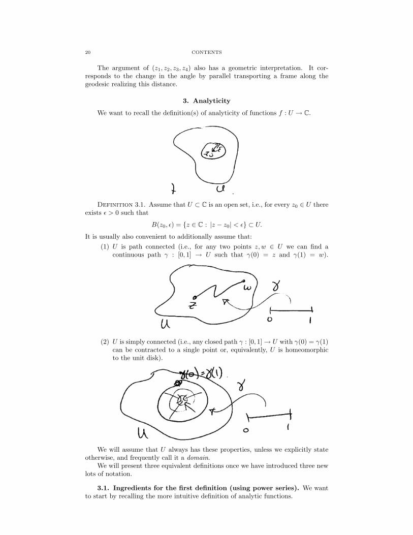
It is usually also convenient to additionally assume that:(1) U is path connected (i.e., for any two points z, w ∈ U we can find a
continuous path γ : [0, 1] → U such that γ(0) = z and γ(1) = w).
(2) U is simply connected (i.e., any closed path γ : [0, 1]→ U with γ(0) = γ(1)can be contracted to a single point or, equivalently, U is homeomorphicto the unit disk).
We will assume that U always has these properties, unless we explicitly stateotherwise, and frequently call it a domain.
We will present three equivalent definitions once we have introduced three newlots of notation.
3.1. Ingredients for the first definition (using power series). We wantto start by recalling the more intuitive definition of analytic functions.
3. ANALYTICITY 21
Definition 3.2. Let z0 ∈ C and let (an)∞n=0 be a sequence of complex numbers.We say that an infinite series
∑∞n=0 an(z − z0)n has a radius of convergence 0 ≤
R ≤ +∞ (at z0) if1R
= lim supn→+∞
|an|1/n . (1)
In particular, we have the folowing:
Lemma 3.3. Assume that R > 0. For any 0 < r < R the series
fz0(z) :=∞∑n=0
an(z − z0)n
converges (uniformly) on B(z0, r) and defines a function.
3.2. Ingredients for the second definition (using complex differentia-bility). We begin by what it means for a function to be differentiable as a complexfunction.
Definition 3.4. Let U be a domain. We say that f : U → C is complexdifferentiable at z0 if the limit
f ′(z0) := limz→z0
f(z)− f(z0)z − z0
exists, i.e., there exists f ′(z0) ∈ C such that for all ε > 0 there exists δ > 0 suchthat if |z − z0| < δ then
|f(z)− f(z0)− (z − z0)f ′(z0)| ≤ ε|z − z0|.
Remark 3.5. The key point is that z can approach z0 in “all directions” as acomplex number.
It is easy to see the following result.
Lemma 3.6. If f is complex differentiable at z0 then it is continuous at z0.
Proof. Given ε > 0 there exists δ > 0 such that whenever |z − z0| < δ thenwe have that ∣∣∣∣f ′(z0)− f(z)− f(z0)
z − z0
∣∣∣∣ < ε.
In particular, for |z − z0| < δ we can bound
|f(z)− f(z0)| ≤ (|f ′(z0)|+ ε)|z − z0| ≤ (|f ′(z0)|+ ε)δ,
which can be made arbitrarily small by choosing δ > 0 appropriately small.
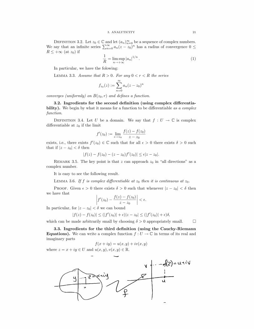
3.3. Ingredients for the third definition (using the Cauchy-RiemannEquations). We can write a complex function f : U → C in terms of its real andimaginary parts
f(x+ iy) = u(x, y) + iv(x, y)where z = x+ iy ∈ U and u(x, y), v(x, y) ∈ R.
22 CONTENTS
Definition 3.7. We say that f : U → C satisfies the Cauchy-Riemann equa-tions if for each z0 = x0 + iy0 ∈ U the partial derivatives
∂u
∂x(x0, y0),
∂u
∂y(x0, y0),
∂v
∂x(x0, y0) and
∂v
∂y(x0, y0)
all exist and satisfy ∂u∂x (x0, y0) = ∂v
∂y (x0, y0) and∂u∂y (x0, y0) = − ∂v
∂x (x0, y0)
for each z0 = x0 + iy0 ∈ U . Equivalently, we can write f(z) = u(x, y) + iv(x, y) and
i∂f
∂x= i
(∂u
∂x+ i
∂v
∂x
)︸ ︷︷ ︸
i ∂v∂y+ ∂u∂y
and∂f
∂y=(∂u
∂y+ i
∂v
∂y
).
using the Cauchy-Riemann equations. Thus we see that
i∂f
∂x=∂f
∂y
Remark 3.8. We can write this as ∂f∂z = 0 using the Wirtinger derivatives
∂f
∂z=
12
(∂f
∂x+ i
∂f
∂y
)and
∂f
∂z=
12
(∂f
∂x− i∂f
∂y
).
4. Definitions of analyticity
We are now in a position to give the equivalent definitions of analyticity.
4.1. The main result. We say that a function f : U → C is analytic if issatisfies any (and thus all) of the following three equivalent conditions.
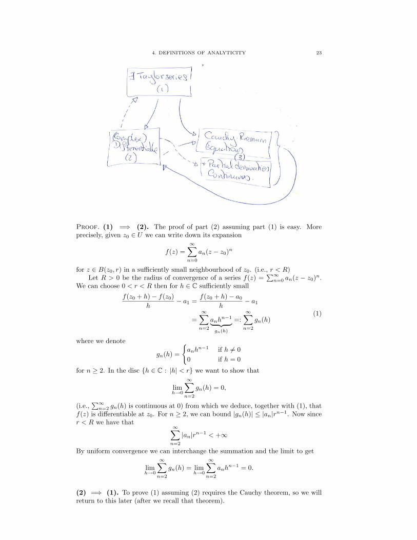
Theorem 4.1. The following are equivalent:
(1) For each z0 ∈ U we can choose ε > 0 and (an)∞n=0 such that the functionf(z) can be represented as a convergent power series about the point z0,i.e.,
f(z) =∞∑n=0
an(z − z0)n
for z ∈ B(z0, ε) ⊂ U and with radius of convergence R > ε > 0;(2) The function f : U → C is complex differentiable at each z0 ∈ U ;(3) The partial derivatives ∂u
∂x , ∂u∂y , ∂v
∂x , ∂v∂y all exist, are continuous and satisfy
the Cauchy-Riemann equations.
We are not yet in a position to prove the theorem completely (since we will stillneed to recall the Cauchy theorem for integrals). However, we will proceed withthe proofs of the parts that we can prove, and then we will return to the remainingparts once we have established Cauchy’s Theorem.
4. DEFINITIONS OF ANALYTICITY 23
Proof. (1) =⇒ (2). The proof of part (2) assuming part (1) is easy. Moreprecisely, given z0 ∈ U we can write down its expansion
f(z) =∞∑n=0
an(z − z0)n
for z ∈ B(z0, r) in a sufficiently small neighbourhood of z0. (i.e., r < R)Let R > 0 be the radius of convergence of a series f(z) =
∑∞n=0 an(z − z0)n.
We can choose 0 < r < R then for h ∈ C sufficiently small
f(z0 + h)− f(z0)h
− a1 =f(z0 + h)− a0
h− a1
=∞∑n=2
anhn−1︸ ︷︷ ︸
gn(h)
=:∞∑n=2
gn(h)(1)
where we denote
gn(h) =
anh
n−1 if h 6= 00 if h = 0
for n ≥ 2. In the disc h ∈ C : |h| < r we want to show that
limh→0
∞∑n=2
gn(h) = 0,
(i.e.,∑∞n=2 gn(h) is continuous at 0) from which we deduce, together with (1), that
f(z) is differentiable at z0. For n ≥ 2, we can bound |gn(h)| ≤ |an|rn−1. Now sincer < R we have that
∞∑n=2
|an|rn−1 < +∞
By uniform convergence we can interchange the summation and the limit to get
limh→0
∞∑n=2
gn(h) = limh→0
∞∑n=2
anhn−1 = 0.
(2) =⇒ (1). To prove (1) assuming (2) requires the Cauchy theorem, so we willreturn to this later (after we recall that theorem).
24 CONTENTS
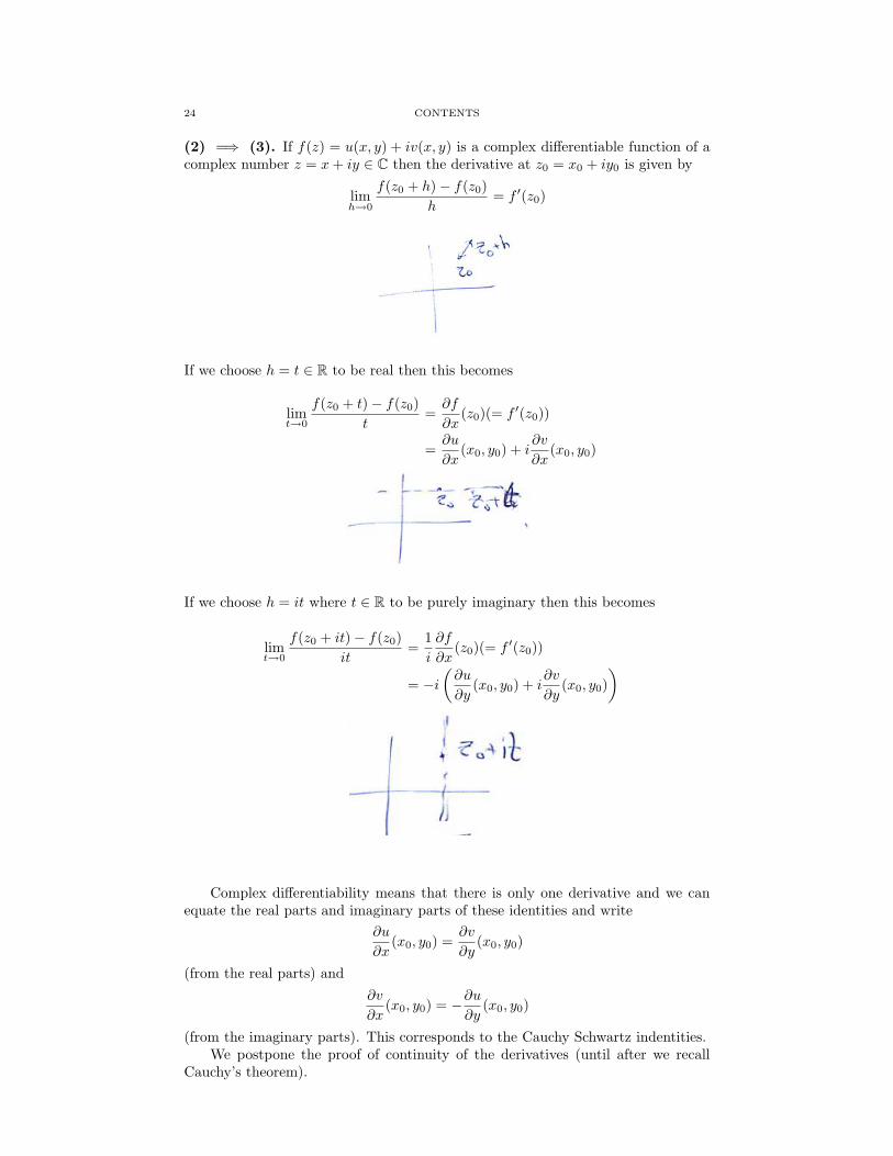
(2) =⇒ (3). If f(z) = u(x, y) + iv(x, y) is a complex differentiable function of acomplex number z = x+ iy ∈ C then the derivative at z0 = x0 + iy0 is given by
limh→0
f(z0 + h)− f(z0)h
= f ′(z0)
If we choose h = t ∈ R to be real then this becomes
limt→0
f(z0 + t)− f(z0)t
=∂f
∂x(z0)(= f ′(z0))
=∂u
∂x(x0, y0) + i
∂v
∂x(x0, y0)
If we choose h = it where t ∈ R to be purely imaginary then this becomes
limt→0
f(z0 + it)− f(z0)it
=1i
∂f
∂x(z0)(= f ′(z0))
= −i(∂u
∂y(x0, y0) + i
∂v
∂y(x0, y0)
)
Complex differentiability means that there is only one derivative and we canequate the real parts and imaginary parts of these identities and write
∂u
∂x(x0, y0) =
∂v
∂y(x0, y0)
(from the real parts) and∂v
∂x(x0, y0) = −∂u
∂y(x0, y0)
(from the imaginary parts). This corresponds to the Cauchy Schwartz indentities.We postpone the proof of continuity of the derivatives (until after we recall
Cauchy’s theorem).
4. DEFINITIONS OF ANALYTICITY 25
(3) =⇒ (2). We can write
f(z)− f(z0)z − z0
=(u(x, y)− u(x0, y0)) + i(v(x, y)− v(x0, y0))
z − z0.
For each |x− x0|, |y − y0| sufficiently small we can write
|u(x, y)− u(x0, y0)− (x− x0)∂u
∂x(x, y0)− (y − y0)
∂u
∂y(x0, y0)|
≤ |x− x0|ε1(x0, y0) + |y − y0|ε1(x, y0), and
|v(x, y)− v(x0, y0) = (x− x0)∂v
∂x(x0, y0) + (y − y0)
∂v
∂y(x, y0)|
≤ |x− x0|ε2(x0, y0) + |y − y0|ε2(x, y0)
by using the triangle inequality
|u(x, y)− u(x0, y0)| ≤ |u(x, y)− u(x, y0)|+ |u(x, y0)− u(x0, y0)| and
|v(x, y)− v(x0, y0)| ≤ |v(x, y)− v(x, y0)|+ |v(x, y0)− v(x0, y0)|
and the mean value theorem, where ε1(·), ε2(·) are bounds on the partial derivatives.Moreover, continuity of the partial derivatives means that ε1(·), ε2(·)→ 0 as z → z0.
Since |x−x0|, |y−y0| ≤ |z−z0| then for |z−z0| sufficiently small we can boundthe differences by
|u(x, y)− u(x0, y0)− (x− x0)∂u
∂x(x0, y0)− (y − y0)
∂u
∂y(x, y0)|
≤ |z − z0| (ε1(x0, y0) + ε1(x, y0)) , and
|v(x, y)− v(x0, y0) = (x− x0)∂v
∂x(x0, y0) + (y − y0)
∂v
∂y(x, y0)|
≤ |z − z0| (ε2(x0, y0) + ε2(x, y0))
(1)
where continuity of the derivatives means that ε1(·), ε2(·) → 0 as (x, y) → (x0, y0).By the Cauchy-Riemann equations we have that
(x− x0)∂u
∂x(x0, y0) + (y − y0)
∂u
∂y(x, y0) + i
((x− x0)
∂v
∂x(x0, y0) + (y − y0)
∂v
∂y(x, y0)
)= (x− x0)
(∂u
∂x(x0, y0) + i
∂v
∂x(x0, y0)
)+ (y − y0)
(∂u
∂y(x0, y0) + i
∂v
∂y(x0, y0)
)︸ ︷︷ ︸
=:− ∂v∂x (x0,y0)+i ∂u∂x (x0,y0)
= (x− x0)(∂u
∂x(x0, y0) + i
∂v
∂x(x0, y0)
)+ (y − y0)
(−∂v∂x
(x0, y0) + i∂u
∂x(x0, y0)
)= ((x− x0) + i(y − y0))
((∂u
∂x(x0, y0) + i
∂v
∂x(x0, y0)
)+(i∂v
∂x(x0, y0) +
∂u
∂x(x0, y0)
))= (z − z0)︸ ︷︷ ︸
(x−x0)+i(y−y0)
(∂u
∂x(x0, y0) + i
∂v
∂x(x0, y0)
)(2)
using the Cauchy-Riemann equations. Comparing (1) and (2) we have that
f(z)− f(z0)z − z0
=(∂u
∂x(x0, y0) + i
∂v
∂x(x0, y0)
)+|z − z0|z − z0
(ε1(·) + iε2(·))
→ ∂u
∂x(x0, y0) + i
∂v
∂x(x0, y0)(= f ′(z0))
as z → z0.

26 CONTENTS
Example 4.2 (Three ways to see f(z) = ez is analytic at z = 0). We letf : C→ C be the exponential map f(z) = ez where z = x+ iy ∈ C.
(1) We can write f(z) =∑∞n=0(−1)n z
n
n! ;(2) We have a complex derivative f ′(z) = ez (which makes sense as a power
series); and(3) We can f(z) = u+ iv = ex cos y + iex sin y. In particular,
∂u
∂x= ex cos y =
∂v
∂yand
∂u
∂y= −ex sin y = −∂v
∂x.
The continuity of the partial derivatives in part (3) of the theorem is crucial.Without the assumption that partial derivatives are continuous, then satisfying theCauchy-Riemann equations is not enough to deduce that f is complex differentiable.
Example 4.3. If f : C→ C is defined by
f(z) =
0 if z = 0exp(−1/z4) otherwise
Thus all the expressions in the Cauchy-Riemann equations are zero, but one canshow that f is not differentiable.
5. Integrals and Cauchy’s Theorem
The most useful theorem in Complex analysis is probably Cauchy’s theorem.
5.1. Integration on piecewise continuous curves. Given a continuouscurve γ : [a, b] → C we can take the real and imaginary parts γ(t) = u(t) + iv(t),where u, v : [a, b]→ R are real valued.
We say that f(t) is differentiable if u, v : [a, b]→ R are differentiable and thenwe define
f ′(t) = u′(t) + iv′(t).
Definition 5.1. If f : [a, b]→ C is continuous then we define∫ b
a
f(t)dt =∫ b
a
u(t)dt+ i
∫ b
a
v(t)dt.
Moreover, for a piecewise continuous function f(t) on a = a0 < a1 < · · · < an = bwe can still define the integral by
n−1∑i=0
∫ ai+1
ai
fdt.
Lemma 5.2. For f, g piecewise continuous on [a, b] and α, β ∈ C we have that:
(1)∫ ba
(αf(t) + βf(t))dt = α∫ baf(t)dt+ β
∫ baf(t))dt
(2) |∫ baf(t)dt| ≤
∫ ba|f(t)|dt
5. INTEGRALS AND CAUCHY’S THEOREM 27
Proof. The first part follows easily from the definitions.For the second part, assume that
∫ baf(t)dt 6= 0 (otherwise the result is trivial)
and we can write reiθ =∫ baf(t)dt. Thus r = |
∫ baf(t)dt| =
∫ bae−iθf(t)dt ∈ R.
Therefore,
r = Re
(∫ b
a
e−iθf(t)dt
)=∫ b
a
Re(e−iθf(t)
)dt ≤
∫ b
a
∣∣e−iθf(t)∣∣ dt =
∫ b
a
|f(t)| dt
and thus
|∫ b
a
f(t)dt| ≤∫ b
a
|f(t)| dt
5.2. parameterization of the curve of integration. If φ : [c, d] → [a, b]is differentiable map with continuous positive derivative so that φ(t) is strictlyincreasing then ∫ b
a
f(s)ds =∫ d
c
f(φ(t))φ′(t)dt
by the substitution law and the change of variables law with s = φ(t).
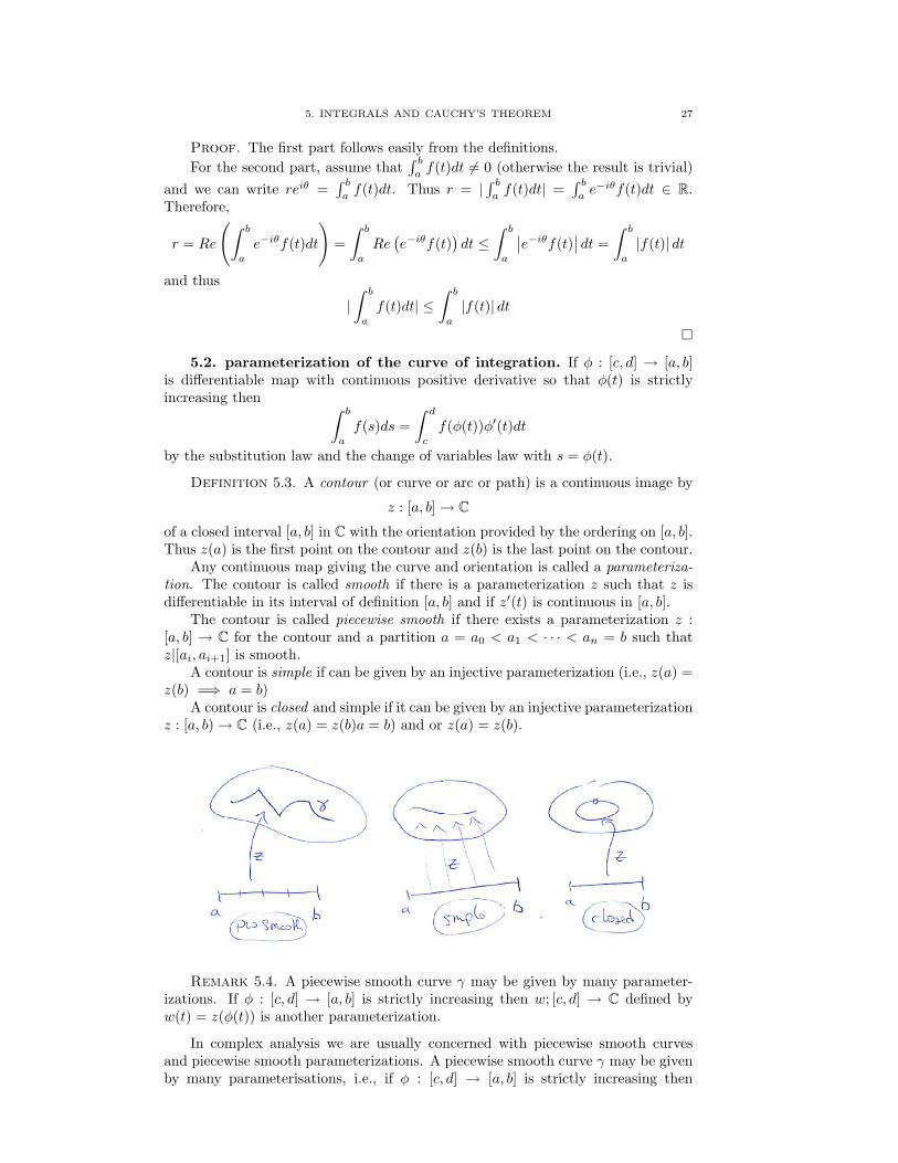
Definition 5.3. A contour (or curve or arc or path) is a continuous image by
z : [a, b]→ C
of a closed interval [a, b] in C with the orientation provided by the ordering on [a, b].Thus z(a) is the first point on the contour and z(b) is the last point on the contour.
Any continuous map giving the curve and orientation is called a parameteriza-tion. The contour is called smooth if there is a parameterization z such that z isdifferentiable in its interval of definition [a, b] and if z′(t) is continuous in [a, b].
The contour is called piecewise smooth if there exists a parameterization z :[a, b] → C for the contour and a partition a = a0 < a1 < · · · < an = b such thatz|[ai, ai+1] is smooth.
A contour is simple if can be given by an injective parameterization (i.e., z(a) =z(b) =⇒ a = b)
A contour is closed and simple if it can be given by an injective parameterizationz : [a, b)→ C (i.e., z(a) = z(b)a = b) and or z(a) = z(b).
Remark 5.4. A piecewise smooth curve γ may be given by many parameter-izations. If φ : [c, d] → [a, b] is strictly increasing then w; [c, d] → C defined byw(t) = z(φ(t)) is another parameterization.
In complex analysis we are usually concerned with piecewise smooth curvesand piecewise smooth parameterizations. A piecewise smooth curve γ may be givenby many parameterisations, i.e., if φ : [c, d] → [a, b] is strictly increasing then
28 CONTENTS
w : [c, d] → C defined by w(t) = z(φ(t)) is also piecewise smooth if z is piecewisesmooth and φ is differentiable with continuous and positive derivative.
Definition 5.5. We say that two parameterizations z and w are equivalent ifthere exists such a φ.
Exercise 5.6. Show that this is an equivalence relation on parameterizations.
Hint. Clearly we can write w φ−1 = z and φ−1 is continuous with positivederivative. Transitivity follows simply.
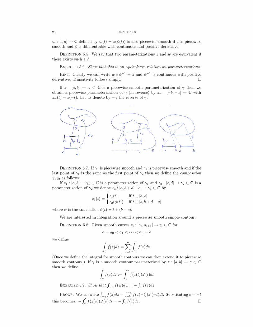
If z : [a, b] → γ ⊂ C is a piecewise smooth parameterization of γ then weobtain a piecewise parameterization of γ (in reverse) by z− : [−b,−a] → C withz−(t) = z(−t). Let us denote by −γ the reverse of γ.
Definition 5.7. If γ1 is piecewise smooth and γ2 is piecewise smooth and if thelast point of γ1 is the same as the first point of γ2 then we define the compositionγ1γ2 as follows:
If z1 : [a, b] → γ1 ⊂ C is a parameterization of γ1 and z2 : [c, d] → γ2 ⊂ C is aparameterization of γ2 we define z3 : [a, b+ d− c]→ γ3 ⊂ C by
z3(t) =
z1(t) if t ∈ [a, b]z2(φ(t)) if t ∈ [b, b+ d− c]
where φ is the translation φ(t) = t+ (b− c).
We are interested in integration around a piecewise smooth simple contour.
Definition 5.8. Given smooth curves zi : [ai, ai+1]→ γi ⊂ C for
a = a0 < a1 < · · · < an = b
we define ∫γ
f(z)dz =n∑i=1
∫γi
f(z)dz.
(Once we define the integral for smooth contours we can then extend it to piecewisesmooth contours.) If γ is a smooth contour parameterized by z : [a, b] → γ ⊂ Cthen we define ∫
γ
f(z)dz :=∫ b
a
f(z(t))z′(t)dt
Exercise 5.9. Show that∫−γ f(w)dw = −
∫γf(z)dz
Proof. We can write∫−γ f(z)dz =
∫ −a−b f(z(−t))z′(−t)dt. Substituting s = −t
this becomes: −∫ baf(z(s))z′(s)ds = −
∫γf(z)dz.
5. INTEGRALS AND CAUCHY’S THEOREM 29
Remark 5.10. More generally, integration with respect to arc length along asimple contour γ is rectifiable if it is given by a continuous map z : [a, b]→ C whichis of bounded variation, i.e., the summations
n−1∑i=0
|z(ai+1)− z(ai)|,
ranging over all partitions a = a0 < a1 < · · · < an = b, is bounded. The supremumof these numbers is by defintion the length of γ. In particular, if γ is smoothrepresented by z : [a, b]→ C then γ is rectifiable and l(γ) =
∫ ba|z′(t)|dt.
The following upper bound is useful.
Lemma 5.11 (Integration along a straight line). If γ is piecewise smooth and fis continuous on γ and |f(z)| ≤M on γ then∣∣∣∣∫
γ
f(z)dz∣∣∣∣ ≤Ml(γ).
Proof. Let z : [a, b]→ γ ⊂ C be a parameterization. Then∣∣∣∣∫γ
f(z)dz∣∣∣∣ =
∣∣∣∣∣∫ b
a
f(z(t))z′(t)dt
∣∣∣∣∣≤∫ b
a
|f(z(t))|.|z′(t)|dt
≤M∫ b
a
|z′(t)|dt = Ml(γ)
as required.
It is useful to illustrate this by a couple of examples .
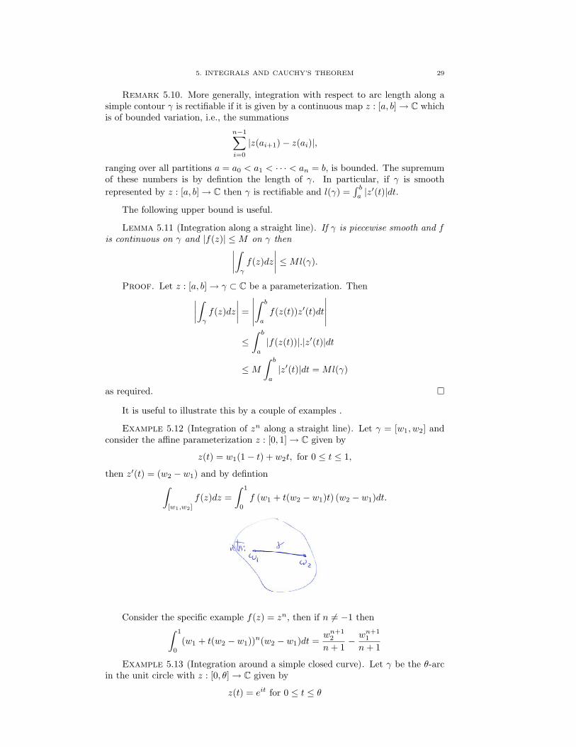
Example 5.12 (Integration of zn along a straight line). Let γ = [w1, w2] andconsider the affine parameterization z : [0, 1]→ C given by
z(t) = w1(1− t) + w2t, for 0 ≤ t ≤ 1,
then z′(t) = (w2 − w1) and by defintion∫[w1,w2]
f(z)dz =∫ 1
0
f (w1 + t(w2 − w1)t) (w2 − w1)dt.
Consider the specific example f(z) = zn, then if n 6= −1 then∫ 1
0
(w1 + t(w2 − w1))n(w2 − w1)dt =wn+1
2
n+ 1− wn+1
1
n+ 1
Example 5.13 (Integration around a simple closed curve). Let γ be the θ-arcin the unit circle with z : [0, θ]→ C given by
z(t) = eit for 0 ≤ t ≤ θ

30 CONTENTS
then z′(t) = ieit and by definition∫γ
f(z)dz =∫ θ
0
enitieitdt.
Consider the specific example f(z) = zn then∫γ
f(z)dz =∫ θ
0
enitieitdt =i
(n+ 1)i
[ei(n+1)t
]θ0
=ei(n+1)θ − 1
n+ 1
if n 6= −1. On the other hand, if n = −1 then one can easily see that∫γ
1zdz =
∫ θ
0
e−itieitdt =∫ θ
0
idt = θi
In particular, if θ = 2π then∫γ
znd =∫ 2π
0
enitieintdt =
0 if n 6= −12πi if n = −1.
5.3. Theorems of Gousart and Cauchy. The last example is a special caseof the following important theorem.
Theorem 5.14 (Gousart’s Theorem). Let f : U → C be an analytic function.Let γ ⊂ U be a closed simple curve then
∫γf(z)dz = 0.
There are two basic approaches to proving this. One approach uses Stokes’theorem, but for variety we will describe the other approach (at least in the contextof γ being a rectangle).
Proof. We begin with a proof of this result in the case that γ is the boundaryof a rectangle R0 = [a, b]× [c, d]. In particular
∂R0 = [a, b]× c ∪ b × [c, d] ∪ [b, a]× d ∪ a × [d, c].
We proceed as follows.
Step 1. We can subdivide R0 into four similar sub-rectangles:
R(1)0 = [a, (a+ b)/2]× [c, (c+ d)/2]
R(2)0 = [(a+ b)/2, b]× [c, (c+ d)/2)]
R(3)0 = [a, (a+ b)/2]× [(c+ d)/2, d]
R(4)0 = [(a+ b)/2, b]× [(c+ d)/2, d]
and then we can write ∫∂R0
f(z)dz =4∑i=1
∫∂R
(i)0
f(z)dz.
(where the integrals along the same curves in different directions cancel).
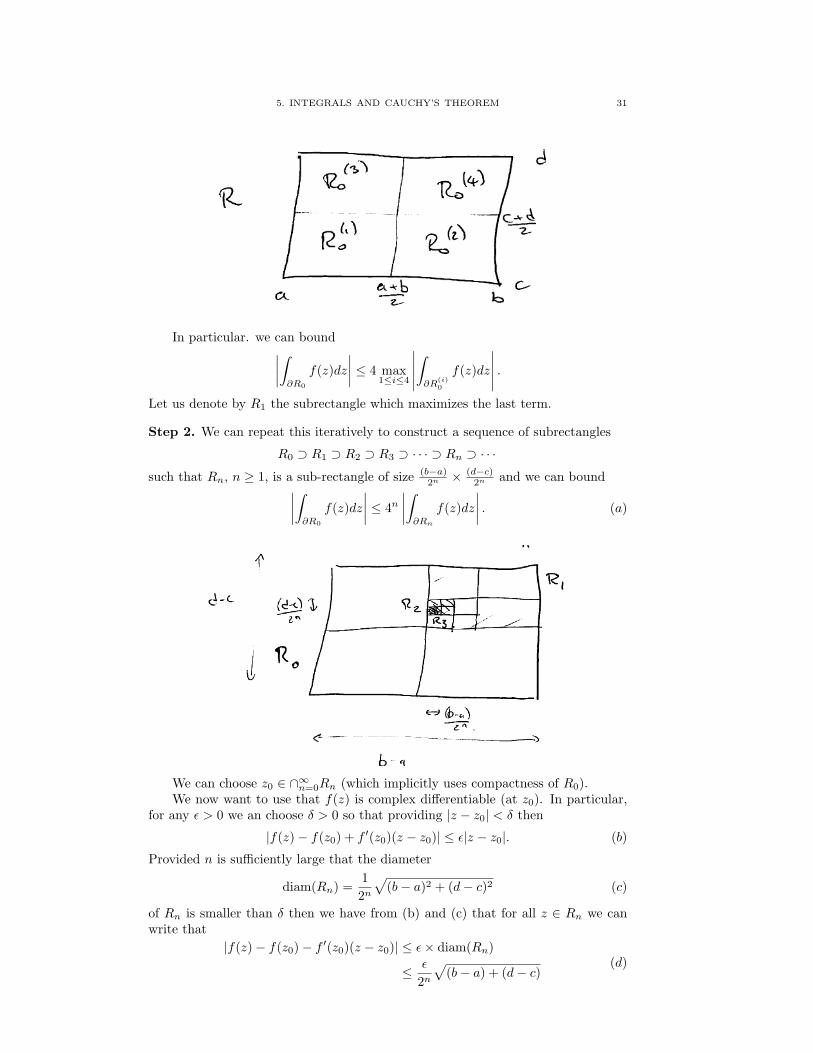
5. INTEGRALS AND CAUCHY’S THEOREM 31
In particular. we can bound∣∣∣∣∫∂R0
f(z)dz∣∣∣∣ ≤ 4 max
1≤i≤4
∣∣∣∣∣∫∂R
(i)0
f(z)dz
∣∣∣∣∣ .Let us denote by R1 the subrectangle which maximizes the last term.
Step 2. We can repeat this iteratively to construct a sequence of subrectangles
R0 ⊃ R1 ⊃ R2 ⊃ R3 ⊃ · · · ⊃ Rn ⊃ · · ·
such that Rn, n ≥ 1, is a sub-rectangle of size (b−a)2n × (d−c)
2n and we can bound∣∣∣∣∫∂R0
f(z)dz∣∣∣∣ ≤ 4n
∣∣∣∣∫∂Rn
f(z)dz∣∣∣∣ . (a)
We can choose z0 ∈ ∩∞n=0Rn (which implicitly uses compactness of R0).We now want to use that f(z) is complex differentiable (at z0). In particular,
for any ε > 0 we an choose δ > 0 so that providing |z − z0| < δ then
|f(z)− f(z0) + f ′(z0)(z − z0)| ≤ ε|z − z0|. (b)
Provided n is sufficiently large that the diameter
diam(Rn) =12n√
(b− a)2 + (d− c)2 (c)
of Rn is smaller than δ then we have from (b) and (c) that for all z ∈ Rn we canwrite that
|f(z)− f(z0)− f ′(z0)(z − z0)| ≤ ε× diam(Rn)
≤ ε
2n√
(b− a) + (d− c)(d)
32 CONTENTS
Moreover, since
length(∂Rn) =12n
(2(b− a) + (d− c)) (e)
we can use (a), (d) and (e) to bound∫∂Rn
(f(z)− f(z0)− f ′(z0)(z − z0))dz
≤ supz∈Rn
|f(z)− f(z0)− f ′(z0)(z − z0)|︸ ︷︷ ︸≤ ε
2n
√(b−a)2+(d−c)2
× length(∂Rn)︸ ︷︷ ︸≤ 1
2n (2(b−a)(d−c))
≤ ε
4n(√
(b− a)2 + (d− c)22((b− a) + (d− c)))
︸ ︷︷ ︸=:C
.
(f)
Step 3. Moreover, we have the following estimates:For each rectangle Rn:(1) We can evaluate
∫∂Rn
1dz = 0;(2) We can evaluate
∫∂Rn
(z − z0)dz = 0.
Proof. The first part is easy, since the contribution to the integrals fromopposite sides cancel. For the second part, we can simply explicitly do the integral.
Comparing (a) and (f) and the above claim we can write:∣∣∣∣∫∂R0
f(z)dz∣∣∣∣ ≤ 4n
∣∣∣∣∫∂Rn
f(z)dz∣∣∣∣
= 4n|∫∂Rn
(f(z)− f(z0)− f ′(z0)(z − z0)) dz −∫∂Rn
(f(z0)− f ′(z0)(z − z0)) dz︸ ︷︷ ︸= 0 (by claim)
|
≤ 4n(C
4nε
)= Cε
Thus, since ε can be chosen arbitrarily small, we finally deduce that∫∂R0
f(z)dz = 0,as required.
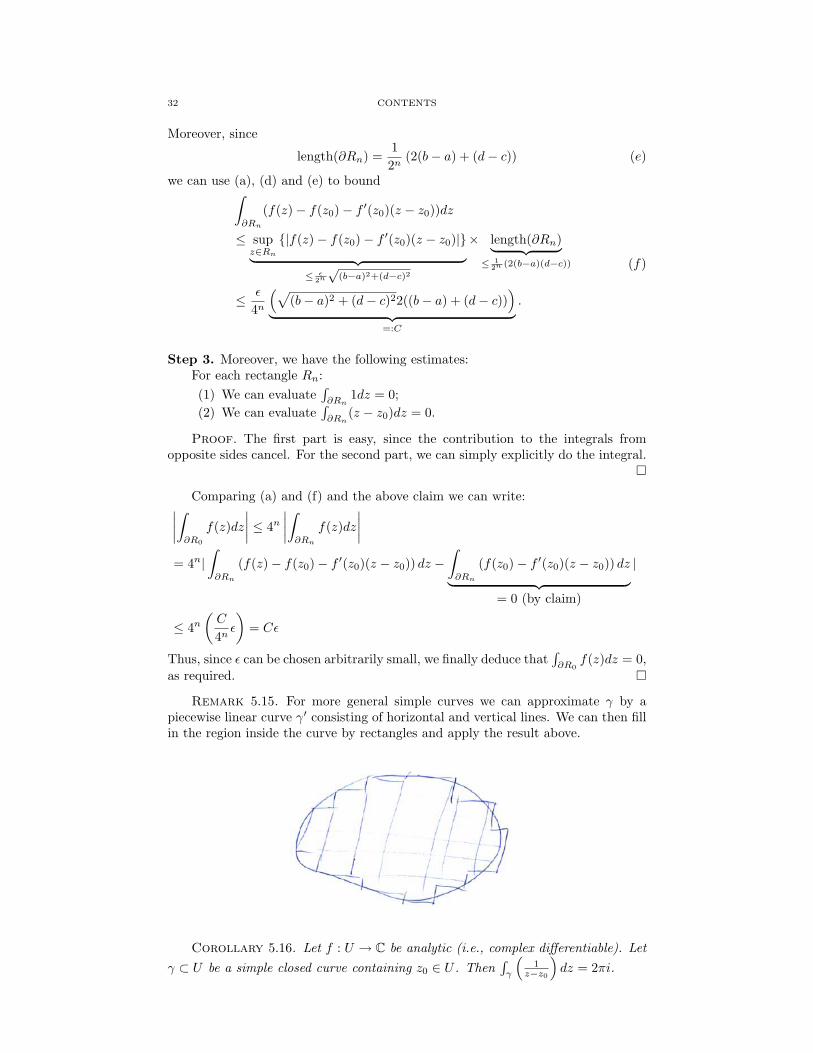
Remark 5.15. For more general simple curves we can approximate γ by apiecewise linear curve γ′ consisting of horizontal and vertical lines. We can then fillin the region inside the curve by rectangles and apply the result above.
Corollary 5.16. Let f : U → C be analytic (i.e., complex differentiable). Letγ ⊂ U be a simple closed curve containing z0 ∈ U . Then
∫γ
(1
z−z0
)dz = 2πi.
5. INTEGRALS AND CAUCHY’S THEOREM 33
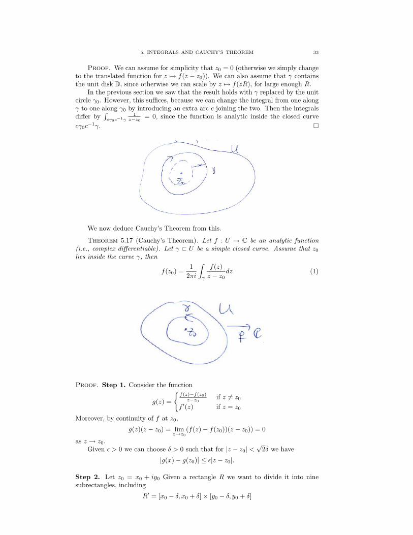
Proof. We can assume for simplicity that z0 = 0 (otherwise we simply changeto the translated function for z 7→ f(z − z0)). We can also assume that γ containsthe unit disk D, since otherwise we can scale by z 7→ f(zR), for large enough R.
In the previous section we saw that the result holds with γ replaced by the unitcircle γ0. However, this suffices, because we can change the integral from one alongγ to one along γ0 by introducing an extra arc c joining the two. Then the integralsdiffer by
∫cγ0c−1γ
1z−z0 = 0, since the function is analytic inside the closed curve
cγ0c−1γ.
We now deduce Cauchy’s Theorem from this.
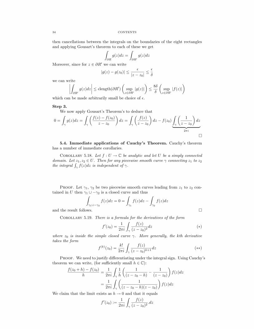
Theorem 5.17 (Cauchy’s Theorem). Let f : U → C be an analytic function(i.e., complex differentiable). Let γ ⊂ U be a simple closed curve. Assume that z0
lies inside the curve γ, then
f(z0) =1
2πi
∫γ
f(z)z − z0
dz (1)
Proof. Step 1. Consider the function
g(z) =
f(z)−f(z0)
z−z0 if z 6= z0
f ′(z) if z = z0
Moreover, by continuity of f at z0,
g(z)(z − z0) = limz→z0
(f(z)− f(z0))(z − z0)) = 0
as z → z0.Given ε > 0 we can choose δ > 0 such that for |z − z0| <
√2δ we have
|g(x)− g(z0)| ≤ ε|z − z0|.
Step 2. Let z0 = x0 + iy0 Given a rectangle R we want to divide it into ninesubrectangles, including
R′ = [x0 − δ, x0 + δ]× [y0 − δ, y0 + δ]
34 CONTENTS
then cancellations between the integrals on the boundaries of the eight rectanglesand applying Gousart’s theorem to each of these we get∫
∂R
g(z)dz =∫∂R′
g(z)dz
Moreover, since for z ∈ ∂R′ we can write
|g(z)− g(z0)| ≤ ε
|z − z0|≤ ε
δ
we can write∣∣∣∣∫∂R′
g(z)dz∣∣∣∣ ≤ εlength(∂R′)
(supz∈∂R′
|g(z)|)≤ 8δ
δ
(supz∈∂R′
|f(z)|)
which can be made arbitrarily small be choice of ε.
Step 3.We now apply Gousart’s Theorem’s to deduce that
0 =∫γ
g(z)dz =∫γ
(f(z)− f(z0)
z − z0
)dz =
∫γ
(f(z)z − z0
)dz − f(z0)
∫γ
(1
z − z0
)dz︸ ︷︷ ︸
2πi
5.4. Immediate applications of Cauchy’s Theorem. Cauchy’s theoremhas a number of immediate corollaries.
Corollary 5.18. Let f : U → C be analytic and let U be a simply connecteddomain. Let z1, z2 ∈ U . Then for any piecewise smooth curve γ connecting z1 to z2
the integral∫γf(z)dz is independent of γ.
Proof. Let γ1, γ2 be two piecewise smooth curves leading from z1 to z2 con-tained in U then γ1 ∪ −γ2 is a closed curve and thus∫
γ1∪−γ2f(z)dz = 0 =
∫γ1
f(z)dz −∫γ2
f(z)dz
and the result follows.
Corollary 5.19. There is a formula for the derivatives of the form
f ′(z0) =1
2πi
∫γ
f(z)(z − z0)2
dz (∗)
where z0 is inside the simple closed curve γ. More generally, the kth derivativetakes the form
f (k)(z0) =k!
2πi
∫γ
f(z)(z − z0)k+1
dz (∗∗)
Proof. We need to justify differentiating under the integral sign. Using Cauchy’stheorem we can write, (for sufficiently small h ∈ C):
f(z0 + h)− f(z0)h
=1
2πi
∫γ
1h
(1
(z − z0 − h)− 1
(z − z0)
)f(z)dz
=1
2πi
∫γ
(1
(z − z0 − h)(z − z0)
)f(z)dz
We claim that the limit exists as h→ 0 and that it equals
f ′(z0) :=1
2πi
∫γ
f(z)(z − z0)2
.dz

5. INTEGRALS AND CAUCHY’S THEOREM 35
To see this we can bound∣∣∣∣f(z0 + h)− f(z0)h
− f ′(z0)∣∣∣∣ ≤ ∣∣∣∣ h2πi
∫γ
(1
(z − z0 − h)(z − z0)2
)f(z)dz
∣∣∣∣|h|2π
(length(γ)
(d(z0, γ)− |h|)d(z0, γ)2
)(supz∈γ|f(z)|
)where d(z0, γ) = infz∈γ |z0− z| and observe that the Right Hand Side tends to zeroas |h| → 0.
The higher derivative formula comes similarly (cf. next application).
Application 5.20 (Completing the equivalence of the definitions of analyticityI: Writing analytic functions as power series). We claim that a complex differentaiblefunction always has a power series expansion.
Let f : U → C be a complex differentiable function function. Let z0 ∈ U andchoose ε > 0 such that
B(z0, ε) = z ∈ C : |z − z0| < R ⊂ U
Choose z ∈ B(z0, ε) and then ρ := |z0− z| < ε and let r be such that ρ < r < ε.Then by Cauchy’s theorem
f(z) =1
2πi
∫C(z0,r)
f(ξ)ξ − z
dξ
where C(z0, r) = z ∈ C : |z − z0| = r is the circle of radius r about z0.
For ρ < |ξ − z0| = r < ε we have that
1ξ − z
=1
(ξ − z0)− (z − z0)
=1
(ξ − z0)(
1− z−z0ξ−z0
)=
1(ξ − z0)
(1 +
(z − z0
ξ − z0
)+(z − z0
ξ − z0
)2
+ · · ·
)
which is uniformly convergent on the circle C(z0, r) since∣∣∣ z−z0ξ−z0
∣∣∣ = ρr < 1. So by
Cauchy’s theorem integrating around C(z0, r) gives
f(z0) =1
2πi
∫C(z0,r)
f(z)(ξ − z0)
dξ
=1
2πi
∫C(z0,r)
f(z)(ξ − z0)
dξ + (z0 − z0)1
2πi
∫C(a,r)
f(z)(ξ − z0)2
dξ
+ (z0 − z0)2 12πi
∫C(a,r)
f(z)(ξ − z0)3
dξ + · · ·
In particular, we can write this as
f(z0) = a0 + a1(z0 − a) + a2(z − a)2 + · · ·
36 CONTENTS
where
an =1
2π
∫C(a,r)
f(z)(ξ − z0)n+1
dξ
and we know the series has Radius of convergence R =(lim supn→+∞ |an|1/n
)−1>
r. Thus f(z) is a power series about a.
Application 5.21 (Completing the equivalence of the definitions of analyticityII: Continuity of the partial derivatives). Let f : U → C be complex differentiable.For z0 ∈ U we can γ ⊂ U be a simple closed curve containing z0. We see from(*) that f ′(z0) depends continuously on the point z0. Furthermore, since complexdifferentability implies that for f(x+ iy) = u(x, y) + iv(x, y) we can write
f ′(z0) =∂u
∂x+ i
∂v
∂x=∂v
∂y− i∂u
∂y
from which we can deduce that the partial derivatives are continuous.
Corollary 5.22. Let f : U → C be analytic and let z0 be a unique zero (ofmultiplicity one). Let γ ⊂ U be a simple closed curve. Then
z0 =1
2πi
∫γ
zf ′(z)f(z)
dz
Proof. We can write f(z) = (z − z0)g(z), where g : U → C where g : U → Cis non-zero and analytic (and, in particular, g(z0) 6= 0). The function f ′(z)
f(z) is ofthe form 1
z−z0 + ψ(z) where ψ : U → C is analytic and given by ψ(z) = g′(z)/g(z).Thus, by Cauchy’s theorem we can write
12πi
∫γ
zf ′(z)f(z)
dz =1
2πi
∫γ
z1
z − z0dz︸ ︷︷ ︸
=z0
+1
2πi
∫γ
zψ(z)dz︸ ︷︷ ︸=0
= z0.
Application 5.23 (Perturbation Theory for eigenvalues of matrices). Assumethat A is a matrix and λA is a simple eigenvalue. Then letting fA(z) = det(zI −A)then we see that z0 is a simple zero for f(z). By the previous corollary, we see that
λA =1
2πi
∫γ
zf ′A(z)fA(z)
dz
However, it is easy to see that the coefficients of the polynomials fA(z) andf ′A(z) depend smoothly on the entries in the matrix A. This is true on γ and thuswe can deduce the same for λA.
5.5. Converse to Cauchy’s Theorem. The following is a converse to Cauchy’sTheorem which is often useful in proofs of later results.
Theorem 5.24 (Moreira’s Theorem). Let U be a domain and let f : U → C becontinuous and satsify
∫∂∆
f(z)dz = 0 for all simple closed curves ∆ ⊂ U . Then fis analytic.
Proof. Fix a point z0 ∈ U . We can define F : U → C by associating to anyz ∈ U a piecewise smooth curve γ parameterized by z : [0, 1] → γ ⊂ C wherez(0) = z0 and z(0) = z and then defining
F (z) =∫γ
f(z)dz.
6. PROPERTIES OF ANALYTIC FUNCTIONS 37
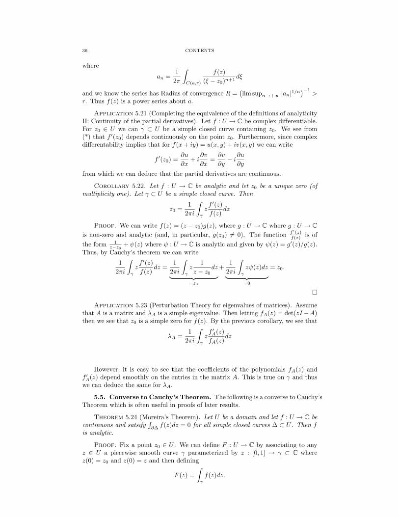
We first observe that since U is a (simply connected) domain this is well defined,since if γ1 is a second path from z0 to z then we have that∫
γ
f(z)dz −∫γ1
f(z)dz =∫γ
f(z)dz +∫−γ1
f(z)dz =∫γ(−γ1)
f(z)dz = 0
since γ(−γ1) is a picewise closed curve, and F : U → C is analytic, and thus we canapply Cauchy’s theorem.
We can now deduce that F ′(z) = f(z), i.e., f is the complex derivative of F .But if F it is complex differentiable then it is analytic, and thus all of the derivativesexist, and us f is also complex differentiable.
6. Properties of analytic functions
We want to find some way to understand better properties of analytic functions.We will begin with properties of individual functions and move onto families of
functions. However, first we have to recall some basic facts.
6.1. Logarithms and roots. Consider the exponential function z 7→ ez forz ∈ C. This is analytic for every z ∈ C. We would like to define the inverse map,the logarithm, in the complex plane but this has a few complications that need tobe addressed.
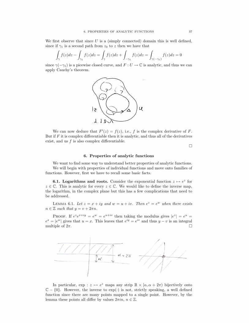
Lemma 6.1. Let z = x + iy and w = u + iv. Then ez = ew when there existsn ∈ Z such that y = v + 2πn.
Proof. If ezex+iy = ew = eu+iv then taking the modulus gives |ez| = eu =ex = |ew| gives that u = x. This leaves that eiy = eiv and thus y − v is an integralmultiple of 2π.
In particular, exp : z 7→ ez maps any strip R × [α, α + 2π) bijectively ontoC − 0. However, the inverse to exp(·) is not, strictly speaking, a well definedfunction since there are many points mapped to a single point. However, by thelemma these points all differ by values 2πin, n ∈ Z.
38 CONTENTS
We would like to write w = log z when z = ew. If w = u + iv and expw = zthen
eueiv = |z| z|z|
= |z|eiθ
for some θ since∣∣∣ z|z| ∣∣∣ = 1. Hence eu = |z| and v = θ + 2πn for any n ∈ Z.
Therefore u = log |z| and w = log |z|+ i(θ + 2πn) for some n ∈ Z.
Definition 6.2. For z 6= 0 define the function arg(z) = arg(z/|z|) = θ ifz/|z| = eiθ and −π ≤ θ < π.
For log(·) there are different branches of arg with different restricted domains.The principle branch of arg is denoted Arg(z) and is such that Arg(eiθ) is the uniquenumber of the form θ + 2πn which lies between −π and π. This is not defined onthe negative real line (−∞, 0].
Returning to the definition of log:
Definition 6.3. The principle branch of log is denoted Log(z) and is of theform log |z|+ iArg(z). This is not defined on the negative real line (−∞, 0].
We can then use exp and Log to define complex powers of complex numbers.In particular, we can write that zw = exp(w.Log(z)).
Example 6.4. Find the value of
(−1− i)1+i := exp ((1 + i)Log(−1− i))
We observe that arg(−i− i) = − 34π and Log(−i− i) = log
√2− 3
4πi. Thus
(−1− i)1+i = exp ((1 + i)Log(−1− i)) = exp((1 + i)(
log√
2− 34πi)).
Example 6.5. If ρ ∈ N then we can write
z1/ρ = exp (log(z)/ρ) = exp ((log |z|+ iArg(z))/ρ)).
If z = reiθ then
z1/ρ = exp((1/ρ)(log r + i(θ + 2πn))) = r1/ρei(θ+2πn)/ρ = r1/ρei(θe2πin)/ρ.
These take the values r1/ρ, r1/ρei2πθ, · · · , r1/ρei(θ+2π(p−1)/p.In particular
z1/2 = exp(
12
log(z))
= exp(
12
log |z|+ 12
arg(z))
= |z|1/2eiArg(z)/2.
More generally, for zq/p we simply replace z by zq.
Remark 6.6. If α is irrational then we can write
zα = exp (α log z) = exp(α log r + αi(θ + 2πn)) .
and the set of values with n ∈ Z is infinite. To see this, let z = reiθ then
exp(αi(θ + 2πn)) = exp(αi(θ + 2πm)) ⇐⇒ exp(αi2π(n−m)) = 1
⇐⇒ α2π(n−m) = 1 ⇐⇒ n = m.
(since α is irrational).

6. PROPERTIES OF ANALYTIC FUNCTIONS 39
6.2. Location of zeros: Argument Principle and Rouche’s Theorem.We can apply Gousart’s and Cauchy’s theorem to prove two useful results
Lemma 6.7. Suppose that f : U → C is analytic and non-zero then there existsan analytic function h : U → C such that eh(z) = f(z) for all z ∈ U .
Proof. Since f is analytic we say that f ′ is analytic and since f does notvanish then f ′/f is analytic and so f ′/f has a primitive h by integrating f , i.e.,h′ = f ′/f for h analytic. Thus
d
dz
(f(z)e−h(z)
)= f ′(z)e−h(z) − f(z)h′(z)e−h(z) = 0
so f(z)e−h(z) = Constant = ea 6= 0. Thus f(z) = ea+h(z)
We can use this lemma to show the following theorem.
Theorem 6.8 (The Argument Principle). Assume f : U → C is analytic andγ ⊂ U is a simple closed curve. The general case is similar. Assume that f has nozeros on γ. Then the number of zeros N inside γ is given by
N =1
2πi
∫γ
f ′(z)f(z)
dz.
Proof. Assume that z0 is a zero of order n ≥ 1 for f(z). Assume for simplicitythat we have no other zeros.
Using the lemma we can then write write f(z) = (z − z0)Neh(z) and then
f ′(z) = (z − z0)Neh(z)h′(z) +N(z − z0)n−1eh(z)
andf ′(z)f(z)
= h′(z) +N
z − z0
Since the first term is analytic simple pole at z0 we can apply Gousart’s theoremto the first term and Cauchy’s theorem to the second term to write
N =1
2πi
∫γ
f ′(z)f(z)
dz.
With more zeroes the argument naturally generalizes.
Example 6.9. Assume f : D→ C has a simple zero at 0 (i.e., N = 1) and thatγ = z : |z| = r with 0 < r < 1. Writing
f(z) =∞∑n=1
anzn and f ′(z) =
∞∑n=1
nan+1zn
(with a0 = 0 and a1 6= 0) we see that
f ′(z)f(z)
=1z
+ g(z)
40 CONTENTS
where g(z) is analytic on a neighbourhood of 0. By Gousart’s theorem∫γg(z)dz = 0
and a direct calculation gives
12πi
∫γ
f ′(z)f(z)
dz =1
2πi
∫γ
1zdz︸ ︷︷ ︸
=1
+1
2πi
∫γ
g(z)dz︸ ︷︷ ︸=0
Application 6.10 (localizing zeros of Riemann Zeta function). One of themajor open problems in mathematics is the Riemann Hypothesis. For s ∈ C withRe(s) > 1 we define the Riemann zeta function
ζ(s) =∞∑n=1
1ns
(It converges since |ζ(s)| ≤∑∞n=1 n
−Re(s) < +∞). Moreover, it has an analyticextension to C− 1, i.e., there is an analytic function f : C− 1 → C such thatf(s) = ζ(s) for Re(s) > 1.
Riemann Hypothesis (Conjecture, 1859) The only zeros for f(s) occur ats = −2,−4,−6, · · · and on the line
L := s =12
+ it : t ∈ R.
This is Hilbert’s 8th problem from his famous list of 23 open problems from 1900,and one of the 7 Millenium problems from 2000 for which the Clay Institute offereda million dollars.
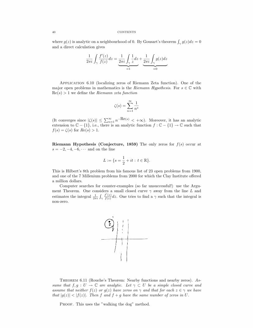
Computer searches for counter-examples (so far unsuccessful!) use the Argu-ment Theorem. One considers a small closed curve γ away from the line L andestimates the integral 1
2πi
∫γf ′(z)f(z) dz. One tries to find a γ such that the integral is
non-zero.
Theorem 6.11 (Rouche’s Theorem: Nearby functions and nearby zeros). As-sume that f, g : U → C are analytic. Let γ ⊂ U be a simple closed curve andassume that neither f(z) or g(z) have zeros on γ and that for each z ∈ γ we havethat |g(z)| < |f(z)|. Then f and f + g have the same number of zeros in U .
Proof. This uses the ”walking the dog” method.
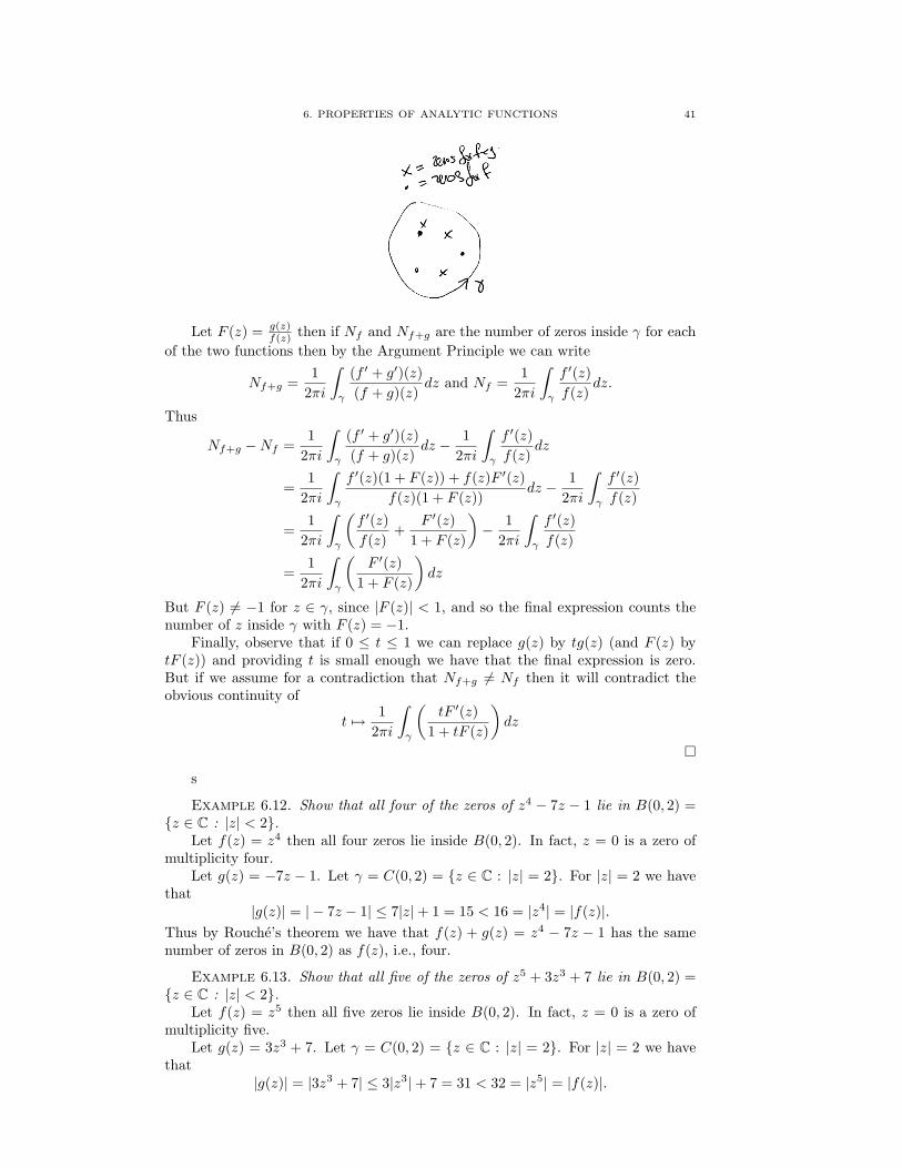
6. PROPERTIES OF ANALYTIC FUNCTIONS 41
Let F (z) = g(z)f(z) then if Nf and Nf+g are the number of zeros inside γ for each
of the two functions then by the Argument Principle we can write
Nf+g =1
2πi
∫γ
(f ′ + g′)(z)(f + g)(z)
dz and Nf =1
2πi
∫γ
f ′(z)f(z)
dz.
Thus
Nf+g −Nf =1
2πi
∫γ
(f ′ + g′)(z)(f + g)(z)
dz − 12πi
∫γ
f ′(z)f(z)
dz
=1
2πi
∫γ
f ′(z)(1 + F (z)) + f(z)F ′(z)f(z)(1 + F (z))
dz − 12πi
∫γ
f ′(z)f(z)
=1
2πi
∫γ
(f ′(z)f(z)
+F ′(z)
1 + F (z)
)− 1
2πi
∫γ
f ′(z)f(z)
=1
2πi
∫γ
(F ′(z)
1 + F (z)
)dz
But F (z) 6= −1 for z ∈ γ, since |F (z)| < 1, and so the final expression counts thenumber of z inside γ with F (z) = −1.
Finally, observe that if 0 ≤ t ≤ 1 we can replace g(z) by tg(z) (and F (z) bytF (z)) and providing t is small enough we have that the final expression is zero.But if we assume for a contradiction that Nf+g 6= Nf then it will contradict theobvious continuity of
t 7→ 12πi
∫γ
(tF ′(z)
1 + tF (z)
)dz
s
Example 6.12. Show that all four of the zeros of z4 − 7z − 1 lie in B(0, 2) =z ∈ C : |z| < 2.
Let f(z) = z4 then all four zeros lie inside B(0, 2). In fact, z = 0 is a zero ofmultiplicity four.
Let g(z) = −7z − 1. Let γ = C(0, 2) = z ∈ C : |z| = 2. For |z| = 2 we havethat
|g(z)| = | − 7z − 1| ≤ 7|z|+ 1 = 15 < 16 = |z4| = |f(z)|.Thus by Rouche’s theorem we have that f(z) + g(z) = z4 − 7z − 1 has the samenumber of zeros in B(0, 2) as f(z), i.e., four.
Example 6.13. Show that all five of the zeros of z5 + 3z3 + 7 lie in B(0, 2) =z ∈ C : |z| < 2.
Let f(z) = z5 then all five zeros lie inside B(0, 2). In fact, z = 0 is a zero ofmultiplicity five.
Let g(z) = 3z3 + 7. Let γ = C(0, 2) = z ∈ C : |z| = 2. For |z| = 2 we havethat
|g(z)| = |3z3 + 7| ≤ 3|z3|+ 7 = 31 < 32 = |z5| = |f(z)|.
42 CONTENTS
Thus by Rouche’s theorem we have that f(z) + g(z) = z5 + 3z3 + 7 has the samenumber of zeros in B(0, 2) as f(z), i.e., five.
Example 6.14. Show that z4 − 7z − 1 has precisely one zero in the unit diskD = z ∈ C : |z| < 1.
Let f(z) = −7z − 1 then f(z) has precisely one zero in D, at z = − 17 .
Let g(z) = z4. Let γ = C(0, 1) = z ∈ C : |z| = 1. For |z| = 1 we have that
|g(z)| = |z4| = 1 < 6 = 7− 1 = |7z| − 1 ≤ | − 7z − 1| = |f(z)|.
Thus by Rouche’s theorem we have that f(z) + g(z) = z4 − 7z − 1 has the samenumber of zeros in D as f(z), i.e., one.
Remark 6.15. There is a more symmetric version of this theorem. If f1 : U →C and f2 : U → C are analytic then |f1(z)− f2(z)| < |f1(z)|+ |f(z)| for z ∈ γ thenf1(z) and f2(z) have the same number of zeros inside the curve.
Corollary 6.16 (Weierstrass-Hurwitz Theorem). Assume fn : U → C are asequence of non-zero analytic functions. If fn converges uniformly on compact setsto a continuous function f (i.e., if K ⊂ U is compact then supz∈K |f(z)−fn(z)| → 0as n→ +∞) then:
(1) f : U → C is analytic(2) f either has no zeros or is identically zero.
Proof. For the first part (due to Weierstrass) one only needs to show that forany simple closed curve γ ⊂ U we have that∣∣∣∣∫
γ
f(z)dz∣∣∣∣ ≤ ∣∣∣∣∫
γ
fn(z)dz∣∣∣∣︸ ︷︷ ︸
=0
+∣∣∣∣∫γ
(f(z)− fn(z))dz∣∣∣∣
≤ 0 + length(γ)(
supz∈K|f(z)− fn(z)|
)︸ ︷︷ ︸
→0
where the first term is zero by Gousart’s theorem (since fn : U → C is analytic).Thus
∫γf(z)dz = 0 for all simple closed curves, and so f is analytic by Moreira’s
Theorem.For the second part (due to Hurwitz), if f(z) isn’t identically zero then the set
of zeros ziNi=1 for f(z) is finite. We need to show that this set is empty. Assumefor a contradiction it isn’t empty and let γ be a closed simple curve which containsone of these zeros z1, say. By Cauchy’s theorem
0 =1
2πi
∫γ
f ′n(z)fn(z)
dz → 12πi
∫γ
f ′(z)f(z)
dz = 1
as n→ +∞ which gives a contradiction.
Application 6.17. Recall that the Riemann zeta function
ζ(s) =∞∑n=1
1ns
was claimed to analytic for Res(s) > 1. To check this we can observe that
fN (s) =N∑n=1
1ns
(=
N∑n=1
exp (−s log n)
)is analytic on C. For any compact set K ⊂ U := s ∈ C : Re(s) > 1, say, we havethat sups∈K |ζ(s)− fn(s)| → 0. Thus by the theorem ζ(s) is analytic on U .
6. PROPERTIES OF ANALYTIC FUNCTIONS 43
6.3. Liouville’s Theorem and the Fundamental Theorem of Algebra.We begin with another application of the Taylor series version of analyticity.
Theorem 6.18 (Liouville’s Theorem). If a function f : C→ C is analytic andbounded then f is constant.
Proof. We can write f(z) as a power series representation centred on 0:
f(z) =∞∑n=0
anzn.
Now we use an estimate for an for any R > 0:
|an| =
∣∣∣∣∣ 12πi
∫C(0,R)
f(z)zn+1
dz
∣∣∣∣∣ ≤ M
Rn+1
2πRπ
=M
Rn
where M is an upper bound for |f(z)| and taking limits as R → ∞ to get an = 0except for n = 0, i.e., f(z) = a0.
Functions which are analytic on all of U = C are called entire functions.
Corollary 6.19 (Fundamental Theorem of algebra). Every non-constant poly-nomial has a root (i.e., a zero, that is there exists z0 such that p(z0) = 0).
Proof. Suppose that the polynomial p(z) does not vanish. Then 1/p(z) isentire and since |p(z)| → +∞ as z → +∞ we have that 1/p(z) → 0 as z → +∞and hence |1/p(z)| < ε for |z| > R and 1/p(z) is bounded for |z| ≤ R so 1/p(z)is bounded throughout C so 1/p(z) is constant, contradicting the fact that p(z) isnon-constant.
In particular, this implies that the polynomial can be written as:
p(z) = anzn + · · ·+ a0 = an(z − z1)(z − z2) · · · (z − zn)
Let z1 be a zero and then write
p(z) = an(z−z1+z1)n+· · ·+a0 = an(z−z1)n+a′n−1(z−z1)n−1+· · ·+a′1(z−z1)+a′0Clearly a′0 = 0, by evaluation at z1. So p(z) = (z−z1)q(z) where q(z) is a polynomialof degree n− 1 (and the leading coefficient of q(z) is 1). Repeating this on q(z) weobtain by induction
p(z) = anzn + · · ·+ a0 = an(z − z1)(z − z2) · · · (z − zn).
6.4. Identity Theorem. The following is an application of the Taylor seriestheorem
Lemma 6.20 (Isolation of zeros). Let r > 0 and let B(z0, r) = z ∈ C : |z−z0| <r. The zeros of a non-trivial f : D(z0, r) → C cannot accumulate within a diskD(z0, r − ε), where ε > 0.
Proof. Assume for a contradiction that zk → w ∈ B(z0, r − ε), for someε > 0, are a convergent sequence of zeros for f(z). We can consider the restrictionf : B(w, ε)→ C and write
f(z) =∞∑n=0
an(z − w)n
satisfies an = 0, for all n ≥ 0, i.e., f(z) is trivial contradicting the hypothesis. Moreprecisely, assume for a contradiction to the claim that for some N ≥ 0 we have thata0 = a1 = · · · = aN−1 = 0 and |an| > 0. Since f(zk) = 0 each k ≥ 1 we can write
f(zk) = 0 =∞∑n=N
an(zk − w)n

44 CONTENTS
If |an| ≤ C(2ε)n, say, then we can bound
0 =
∣∣∣∣∣∞∑n=N
an(zk − w)n∣∣∣∣∣ ≥ |an| − C
∞∑n=N
(r|zk − w|)n = |an| − C2ε|zk − w|)N
1− 2ε|zk − w|
Providing k is sufficiently large the right hand side is positive, giving a contradiction.
Theorem 6.21 (Identity Theorem). Suppose that f, g : U → C are analyticin the domain U and suppose that zn, z0 ∈ U and zn → z0 with zn 6= z0 withf(zn) = g(zn).
Proof. We have already proved this for a disk with centre z0, say, by theprevious lemma, we see that f = g on a disk with centre z0 contained in U .
Let z1 ∈ U then we can see that f(z1) = g(z1) by parameterizing a polynomialline from z0 to z1. Otherwise let w be a point on this line such that f(z) = g(z)for all points from z0 up to w and for some points arbitrarily close to w we havef(z) 6= g(z). But w is the limit of a sequence wn of points with f(wn) = g(wn)and so f = g in a disk cntred at w
This contradicts the definition of w if w is before z1. Hence z1 = w andf(z1) = g(z1).
Corollary 6.22 (Isolation of values). Let f : U → R be analytic and non-constant. Let λ ∈ C then for each z0 ∈ U there exists a punctured disc P (z0, r) =z ∈ C : |z0 − z| < r − z0 such that f(z) 6= λ.
Proof. Assume for a contradiction that for every small punctured disk ofradius r = 1/n, say, there exists zn ∈ P (z0, 1/n) such that f(zn) = λ. But thisimplies f(z) = λ on U , i.e., f(z) is constant and contradicts the hypothesis.
Corollary 6.23 (Open Mapping Theorem). Let f : U → R be a non-constantanalytic function. Then the image f(V ) of any open set V ⊂ U is again an openset.
Remark 6.24. This is very different to case for R. Consider f : R→ R definedby f(x) = x2 is not an open map since, for example, f((−1, 1)) = [0, 1), which isnot open.
Proof. Let z0 ∈ V then it is enough to show that there exists ε > 0 such thatB(f(z0), δ) ⊂ f(V ).
Let g(z) = f(z) − f(z0) then g(z0) = 0. Moreover, z0 must be a simple zero(i.e., multiplicity one) for g otherwise the function g(z) (and hence f(z)) would bea constant function. In particular, there is a simple closed curve γ about z0 andwithin V , containing which z0 as the unique zero. Moreover, by taking the curvesmaller (if necessary) we can assume that g′(z) = f ′(z) has no zeros within γ. Bythe Argument theorem we see that
1 =1
2πi
∫γ
g′(ξ)g(ξ)
dξ =1
2πi
∫γ
f ′(ξ)f(ξ)− f(z0)
dξ.
Moreover, for γ fixed, this remains true if we replace f(z0) by f(z) with |f(z) −f(z0)| < δ, for sufficiently small δ > 0. i.e, for such f(z) ∈ B(f(z0), δ) there existsa unique w inside γ, and thus in V .
6.5. Families of functions and Montel’s Theorem. Recall that a set K ⊂C is compact if and only if it is closed and bounded.
Definition 6.25. Let fn∞n=1 be a family of continuous functions fn : U → C,for n ≥ 1. We say that this family is normal if there is a subsequence fnk∞k=1 whichconverges uniformly on every compact subset of U to a continuous function f : U →
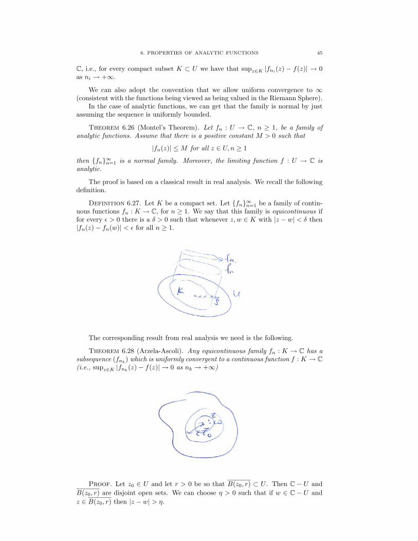
6. PROPERTIES OF ANALYTIC FUNCTIONS 45
C, i.e., for every compact subset K ⊂ U we have that supz∈K |fni(z) − f(z)| → 0as ni → +∞.
We can also adopt the convention that we allow uniform convergence to ∞(consistent with the functions being viewed as being valued in the Riemann Sphere).
In the case of analytic functions, we can get that the family is normal by justassuming the sequence is uniformly bounded.
Theorem 6.26 (Montel’s Theorem). Let fn : U → C, n ≥ 1, be a family ofanalytic functions. Assume that there is a positive constant M > 0 such that
|fn(z)| ≤M for all z ∈ U, n ≥ 1
then fn∞n=1 is a normal family. Moreover, the limiting function f : U → C isanalytic.
The proof is based on a classical result in real analysis. We recall the followingdefinition.
Definition 6.27. Let K be a compact set. Let fn∞n=1 be a family of contin-uous functions fn : K → C, for n ≥ 1. We say that this family is equicontinuous iffor every ε > 0 there is a δ > 0 such that whenever z, w ∈ K with |z − w| < δ then|fn(z)− fn(w)| < ε for all n ≥ 1.
The corresponding result from real analysis we need is the following.
Theorem 6.28 (Arzela-Ascoli). Any equicontinuous family fn : K → C has asubsequence (fnk) which is uniformly convergent to a continuous function f : K → C(i.e., supz∈K |fnk(z)− f(z)| → 0 as nk → +∞)
Proof. Let z0 ∈ U and let r > 0 be so that B(z0, r) ⊂ U . Then C − U andB(z0, r) are disjoint open sets. We can choose η > 0 such that if w ∈ C − U andz ∈ B(z0, r) then |z − w| > η.
46 CONTENTS
If z ∈ B(z0, η) then we can consider restriction fn : B(z0, r) → C and byCauchy’s Theorem
|f ′(z)| =
∣∣∣∣∣ 12πi
∫|z0−z|=ρ
f(z)(z − z0)2
dz
∣∣∣∣∣ ≤ M
ρ
Thus for any z1, z2 ∈ B(z0, η) we have that
|fn(z1)− fn(z2)| ≤
(sup
|z|∈B(z0,η)
|f(z)|
)|z1 − z2|.
In particular, we see that the restrictions fn : B(z0, η) → C, n ≥ 1, form anequicontinuous family. Given ε > 0 we simply choose δ = ε
C > 0.
If K ⊂ U is compact we can cover it be finitely many such balls and we againdeduce that fn : K → C, n ≥ 1, forms an equicontinuous family. We can theninvoke the Arzela-Ascoli theorem to deduce that there is a convergent subsequencefnk : K → C, for k ≥ 1.
The analyticity of the function f : U → C follows from the Hurwitz-Weiestrausstheorem.
Remark 6.29. There is a stronger version which says that fn : U → C, n ≥ 1,is a normal value if they all omit the same three values.
Application 6.30 (Julia sets). Let f : C → C be a polynomial (or, moregenerally, a rational map).
Definition. We say that z ∈ C is in the Fatou set F if there exists ε > 0 such thatthe compositions fn : B(z0, ε)→ C : n ≥ 1 is a normal family.
We define the Juia set J to be the complement of the Fatou set J = C−F .
Example. If f(z) = z2 then fn(z) = z2n . Thus on U∞ = z ∈ C : |z| > 1| wehave that fn(z) → +∞, i.e., the family of iterates converge to ∞. On the otherhand, on U0 = z ∈ C : |z| < 1| we have that fn(z)→ 0, i.e., the family of iteratesconverge to ∞. Thus the Fatou set contains U∞ ∪ U0. But if |z| = 1 then in anydisk B(z, ε) those points also inside the unit disk will converge to 0 while thosepoints also outside the unit disk will converge to ∞. i.e., fn(z) doesn’t converge toan analytic function on B(z, ε).
Therefore F = U∞ ∪U0 and J = C(0, 1). The Julia set is closed, bounded andf(J) = J .
Theorem 6.31. The Julia set consists precisely of those points z ∈ C such thatfor every ε > 0 there exists w ∈ B(z, ε) such that fn(w)→ +∞.
Proof. Assume that for every ε > 0 there exists w ∈ B(z, ε) such thatfn(w) → +∞. Since fn(z) ∈ J is bounded, we cannot have fn : B(z, ε) → Cisn’t normal and thus z ∈ J .
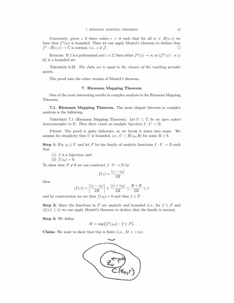
7. RIEMANN MAPPING THEOREM 47
Conversely, given z if there exists ε > 0 such that for all w ∈ B(z, ε) wehave that fn(w) is bounded. Thus we can apply Montel’s theorem to deduce thatfn : B(z, ε)→ C is normal, i.e., z 6∈ J .
Exercise: If f is a polynomial and z ∈ C then either fn(z)→∞ or fn(z) : n ≥0 is a bounded set.
Theorem 6.32. The Julia set is equal to the closure of the repelling periodicpoints.
The proof uses the other version of Montel’s theorem.
7. Riemann Mapping Theorem
One of the most interesting results in complex analysis is the Riemann MappingTheorem.
7.1. Riemann Mapping Theorem. The most elegant theorem in complexanalysis is the following.
Theorem 7.1 (Riemann Mapping Thoerem). Let U ⊂ C be an open subsethomeomorphic to D. Then there exists an analytic bijection f : U → D.
Proof. The proof is quite elaborate, so we break it down into steps. Weassume for simplicity that U is bounded, i.e., U ⊂ B(z0, R) for some R > 0.
Step 1: Fix z0 ∈ U and let F be the family of analytic functions f : U → D suchthat
(1) f is a bijection; and(2) f(z0) = 0.
To show that F 6= ∅ we can construct f : U → D by
f(z) =(z − z0)
2Rthen
|f(z)| =∣∣∣∣ (z − z0)
2R
∣∣∣∣ ≤ |z|+ |z0|2R
≤ R+R
2R≤ 1
and by construction we see that f(z0) = 0 and thus f ∈ F .
Step 2: Since the functions in F are analytic and bounded (i.e., for f ∈ F and|f(z)| ≤ 1) we can apply Montel’s theorem to deduce that the family is normal.
Step 3: We defineM = sup|f ′(z0)| : f ∈ F.
Claim: We want to show that this is finite (i.e., M < +∞).
48 CONTENTS
Proof of Claim: Choose r > 0 sufficiently small that B(z0, r) ⊂ U . By Cauchy’stheorem we have that for any f ∈ F ,
|f ′(z0)| =
∣∣∣∣∣ 12πi
∫|z−z0|=r
f(z)(z − z0)2
dz
∣∣∣∣∣ ≤ 1r
(supz∈D|f(z)|
)︸ ︷︷ ︸
≤1
≤ 1r.
Thus the result follows with M ≤ 1r .
Step 4: We now want to show the supremum is realized.
Claim: There exists f0 ∈ F such that f ′0(z0) = M .
Proof of Claim: We can chose fn ∈ F , n ≥ 1, such that |f ′n(z0)| →M as n→ +∞.By Montel’s Theorem applied to fn we can choose a subsequence fnk∞k=1 andan analytic function f : U → C such that fnk → f uniformly on any compact setK ⊂ C. Therefore, we see that |f ′(z0)| = M .
If we replace f(z) by eiθf(z) then we can choose 0 ≤ θ < 2π so that f ′(z0) = M .
Step 5: We want to show that f : U → D is injective.
Claim: f : U → D is injective.
Proof of Claim: Let z1 6= z2 be distinct points in U . Let 0 < ρ = |z1 − z2| anddefine gk : B(z2, ρ)→ C by
gk(z) = fnk(z)− fnk(z1)
Since the functions fnk(∈ F) are all injective, the functions gk are all non-zero onB(z2, ρ) (i.e., 6 ∃z ∈ B(z2, ρ) with f(z) = 0).
By the Hurwitz-Weierstrauss theorem the limit function g(z) = f(z)− f(z1) iseither identically zero or has no zeros. But, it cannot be identically zero (since weassume that |f ′(z0)| = M > 0). Thus f(z) 6= f(z1) for all z ∈ B(z2, ρ) and thusf(z2) 6= f(z1).
Step 6: We want to show that f : U → D is surjective.
Claim: f : U → D is surjective.
Proof of Claim: Assume for a contradiction that f is not surjective, and thus thereexists w ∈ D which is not in the image f(U).
We can choose a Mobius map φw : D→ D by
φw(z) =z − w1− zw
which maps w to 0. We then consider φw f : U → D. This map now doesn’t have0 in its image. As we saw in a previous lemma, we can write φw f(z) = ek(z) wherek : U → C is analytic, and thus we can define g : U → C by
g(z) = (φw f(z))1/2(=: ek(z)/2).
In particular, g : U → D is one-to-one. Finally, we introduce
φg(z0)(z) =z − g(z0)1− zg(z0)
and define ρ : U → D by ρ(z) = φg(z0) g(z0).We can then compute
ρ′(z0) = φ′g(z0)(g(z0))︸ ︷︷ ︸= 1
1−|g(z0)|2
.g′(z0) (1)
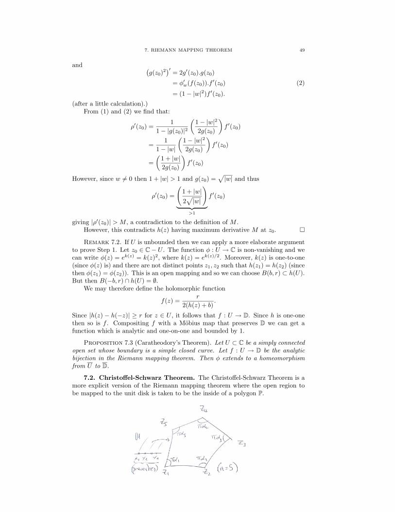
7. RIEMANN MAPPING THEOREM 49
and (g(z0)2
)′= 2g′(z0).g(z0)
= φ′w(f(z0)).f ′(z0)
= (1− |w|2)f ′(z0).
(2)
(after a little calculation).)From (1) and (2) we find that:
ρ′(z0) =1
1− |g(z0)|2
(1− |w|2
2g(z0)
)f ′(z0)
=1
1− |w|
(1− |w|2
2g(z0)
)f ′(z0)
=(
1 + |w|2g(z0)
)f ′(z0)
However, since w 6= 0 then 1 + |w| > 1 and g(z0) =√|w| and thus
ρ′(z0) =
(1 + |w|2√|w|
)︸ ︷︷ ︸
>1
f ′(z0)
giving |ρ′(z0)| > M , a contradiction to the definition of M .However, this contradicts h(z) having maximum derivative M at z0.
Remark 7.2. If U is unbounded then we can apply a more elaborate argumentto prove Step 1. Let z0 ∈ C− U . The function φ : U → C is non-vanishing and wecan write φ(z) = ek(z) = k(z)2, where k(z) = ek(z)/2. Moreover, k(z) is one-to-one(since φ(z) is) and there are not distinct points z1, z2 such that h(z1) = h(z2) (sincethen φ(z1) = φ(z2)). This is an open mapping and so we can choose B(b, r) ⊂ h(U).But then B(−b, r) ∩ h(U) = ∅.
We may therefore define the holomorphic function
f(z) =r
2(h(z) + b).
Since |h(z) − h(−z)| ≥ r for z ∈ U , it follows that f : U → D. Since h is one-onethen so is f . Compositing f with a Mobius map that preserves D we can get afunction which is analytic and one-on-one and bounded by 1.
Proposition 7.3 (Caratheodory’s Theorem). Let U ⊂ C be a simply connectedopen set whose boundary is a simple closed curve. Let f : U → D be the analyticbijection in the Riemann mapping theorem. Then φ extends to a homeomorphismfrom U to D.
7.2. Christoffel-Schwarz Theorem. The Christoffel-Schwarz Theorem is amore explicit version of the Riemann mapping theorem where the open region tobe mapped to the unit disk is taken to be the inside of a polygon P.

50 CONTENTS
We recall that the map w = f(z) = i 1−z1+z maps the unit disk to the upper half
plane H2.Thus it suffices to find a map g : H→ P which is analytic and then gf : D→ P.The general result is the following:
Theorem 7.4 (Schwarz-Christoffel transform). Let P be a polygon with n sidessuch that the internal angles are πα1, · · · , παn. There exist w1, · · · , wn ∈ R suchthat if we consider the function
F (w) =C
(w − w1)1−α1(w − w2)1−α2 · · · (w − wn)1−αn(1)
then for z0 ∈ H we can choose A, C such that f(z) := A+∫ zz0F (w)dw is an analytic
bijection from H to the interior of the polygon P (and which extends continuouslyto the boundary, taking points w1, · · · , wk to the vertices of P).
Here C changes the size and orientation of the image and A translates it.
Remark 7.5. Since the external angles of the polygon sum to (n− 2)π we seethat
n∑i=1
(1− αi) = −2.
Remark 7.6. It is often convenient to consider the case in which the point atinfinity of the w plane maps to one of the vertices of the polygon (e.g., x1 =∞ andthe vertex with angle α1). If this is done, the first factor in the formula is effectivelya constant and may be regarded as being absorbed into the constant C
The following general result is often useful. Let H = z ∈ C : Im(z) > 0 andH− = z ∈ C : Im(z) < 0.
Lemma 7.7 (Schwarz-reflection principle). If g : H→ C is analytic and extendscontinuously to [a, b] ⊂ R such that g([a, b]) ⊂ R then g has an extension as ananalytic function to H ∪ [a, b] ∪H−.
Proof. For z ∈ H we have that z ∈ H− and we define g(z) = g(z). To deduceanalyticity we can use Moreira’s theorem. For example, If γ is a closed curve thatcrosses [a, b] then we can consider two loops γ1, γ2 consisting of the pieces of γin each half-plane plus a subinterval of [a, b] between their intersection points. Byapproximating them by curves wholly in the half planes we see that
∫γ1f(z)dz = 0
and∫γ2f(z)dz = 0, and thus
∫γfdz =
∫γ1f(z)dz +
∫γ2f(z)dz = 0. Thus Moreira’s
Theorem applies and we are done.
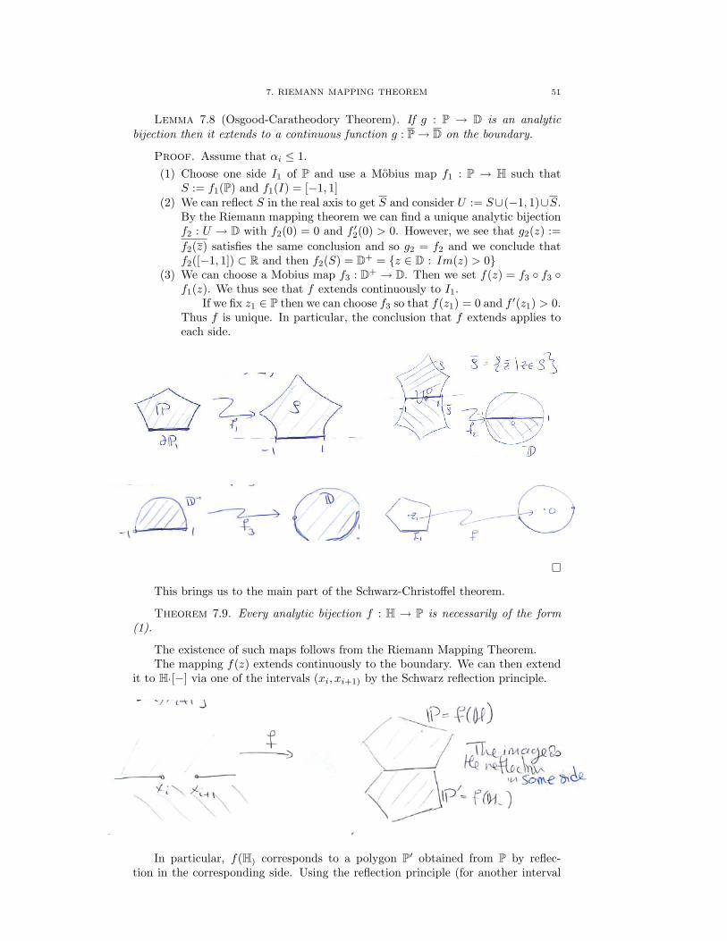
7. RIEMANN MAPPING THEOREM 51
Lemma 7.8 (Osgood-Caratheodory Theorem). If g : P → D is an analyticbijection then it extends to a continuous function g : P→ D on the boundary.
Proof. Assume that αi ≤ 1.(1) Choose one side I1 of P and use a Mobius map f1 : P → H such that
S := f1(P) and f1(I) = [−1, 1](2) We can reflect S in the real axis to get S and consider U := S∪(−1, 1)∪S.
By the Riemann mapping theorem we can find a unique analytic bijectionf2 : U → D with f2(0) = 0 and f ′2(0) > 0. However, we see that g2(z) :=f2(z) satisfies the same conclusion and so g2 = f2 and we conclude thatf2([−1, 1]) ⊂ R and then f2(S) = D+ = z ∈ D : Im(z) > 0
(3) We can choose a Mobius map f3 : D+ → D. Then we set f(z) = f3 f3 f1(z). We thus see that f extends continuously to I1.
If we fix z1 ∈ P then we can choose f3 so that f(z1) = 0 and f ′(z1) > 0.Thus f is unique. In particular, the conclusion that f extends applies toeach side.
This brings us to the main part of the Schwarz-Christoffel theorem.
Theorem 7.9. Every analytic bijection f : H → P is necessarily of the form(1).
The existence of such maps follows from the Riemann Mapping Theorem.The mapping f(z) extends continuously to the boundary. We can then extend
it to H‘[−] via one of the intervals (xi, xi+1) by the Schwarz reflection principle.
In particular, f(H) corresponds to a polygon P′ obtained from P by reflec-tion in the corresponding side. Using the reflection principle (for another interval
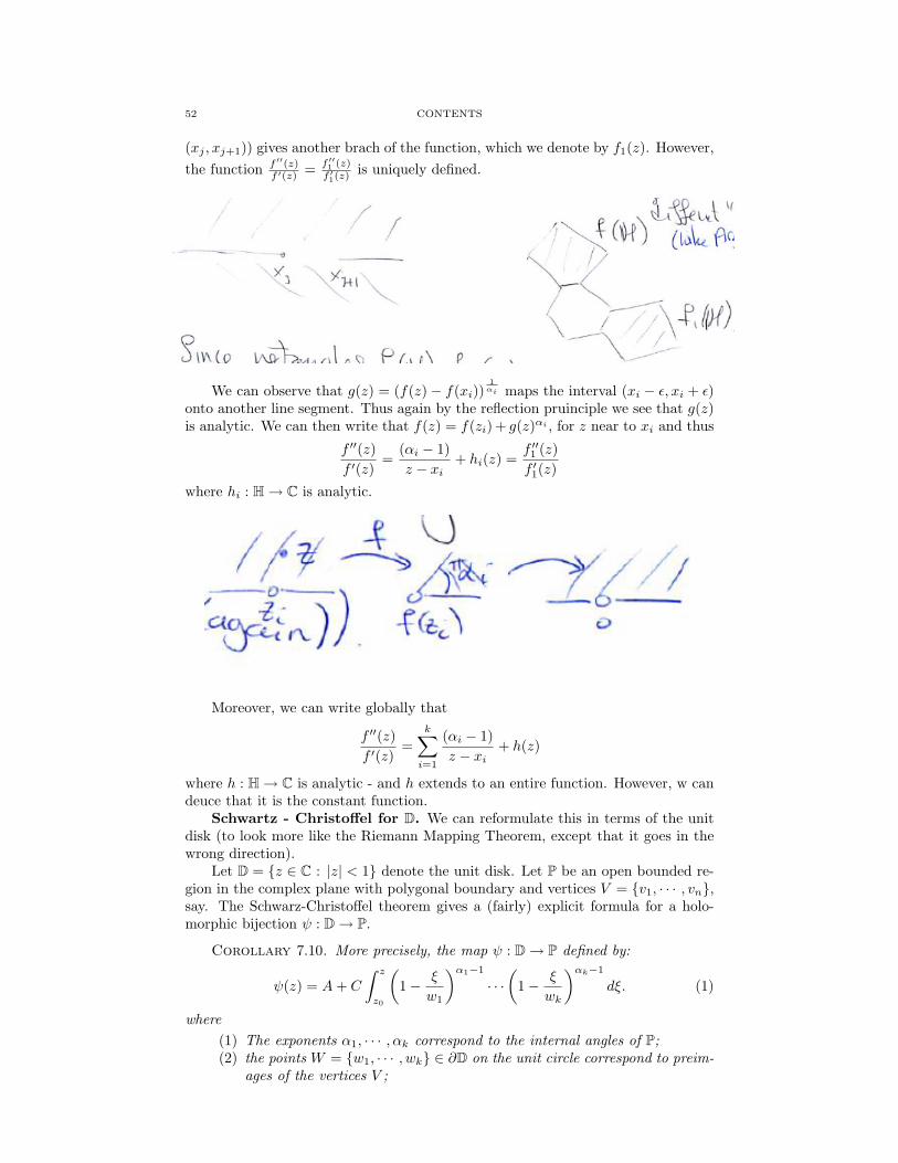
52 CONTENTS
(xj , xj+1)) gives another brach of the function, which we denote by f1(z). However,the function f ′′(z)
f ′(z) = f ′′1 (z)f ′1(z) is uniquely defined.
We can observe that g(z) = (f(z)− f(xi))1αi maps the interval (xi − ε, xi + ε)
onto another line segment. Thus again by the reflection pruinciple we see that g(z)is analytic. We can then write that f(z) = f(zi) + g(z)αi , for z near to xi and thus
f ′′(z)f ′(z)
=(αi − 1)z − xi
+ hi(z) =f ′′1 (z)f ′1(z)
where hi : H→ C is analytic.
Moreover, we can write globally that
f ′′(z)f ′(z)
=k∑i=1
(αi − 1)z − xi
+ h(z)
where h : H→ C is analytic - and h extends to an entire function. However, w candeuce that it is the constant function.
Schwartz - Christoffel for D. We can reformulate this in terms of the unitdisk (to look more like the Riemann Mapping Theorem, except that it goes in thewrong direction).
Let D = z ∈ C : |z| < 1 denote the unit disk. Let P be an open bounded re-gion in the complex plane with polygonal boundary and vertices V = v1, · · · , vn,say. The Schwarz-Christoffel theorem gives a (fairly) explicit formula for a holo-morphic bijection ψ : D→ P.
Corollary 7.10. More precisely, the map ψ : D→ P defined by:
ψ(z) = A+ C
∫ z
z0
(1− ξ
w1
)α1−1
· · ·(
1− ξ
wk
)αk−1
dξ. (1)
where(1) The exponents α1, · · · , αk correspond to the internal angles of P;(2) the points W = w1, · · · , wk ∈ ∂D on the unit circle correspond to preim-
ages of the vertices V ;
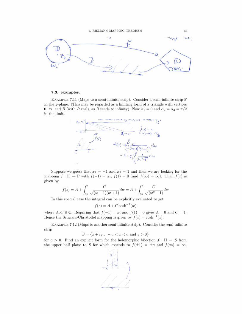
7. RIEMANN MAPPING THEOREM 53
7.3. examples.
Example 7.11 (Maps to a semi-infinite strip). Consider a semi-infinite strip Pin the z-plane. (This may be regarded as a limiting form of a triangle with vertices0, πi, and R (with R real), as R tends to infinity). Now α1 = 0 and α2 = α3 = π/2in the limit.
Suppose we guess that x1 = −1 and x2 = 1 and then we are looking for themapping f : H → P with f(−1) = πi, f(1) = 0 (and f(∞) = ∞). Then f(z) isgiven by
f(z) = A+∫ z
z0
C√(w − 1)(w + 1)
dw = A+∫ z
z0
C√(w2 − 1)
dw
In this special case the integral can be explicitly evaluated to get
f(z) = A+ C cosh−1(w)
where A,C ∈ C. Requiring that f(−1) = πi and f(1) = 0 gives A = 0 and C = 1.Hence the Schwarz-Christoffel mapping is given by f(z) = cosh−1(z).
Example 7.12 (Maps to another semi-infinite strip). Consider the semi-infinitestrip
S = x+ iy : − a < x < a and y > 0for a > 0. Find an explicit form for the holomorphic bijection f : H → S fromthe upper half plane to S for which extends to f(±1) = ±a and f(∞) = ∞.
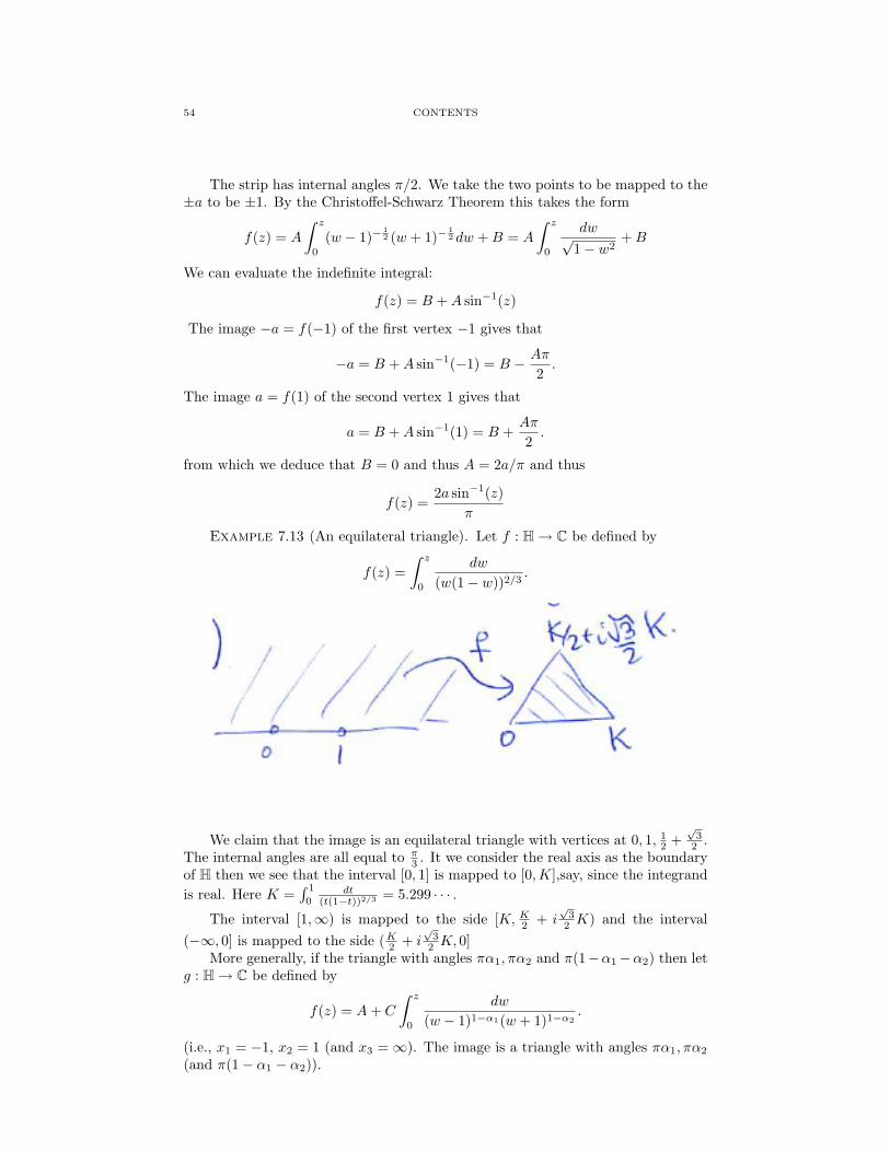
54 CONTENTS
The strip has internal angles π/2. We take the two points to be mapped to the±a to be ±1. By the Christoffel-Schwarz Theorem this takes the form
f(z) = A
∫ z
0
(w − 1)−12 (w + 1)−
12 dw +B = A
∫ z
0
dw√1− w2
+B
We can evaluate the indefinite integral:
f(z) = B +A sin−1(z)
The image −a = f(−1) of the first vertex −1 gives that
−a = B +A sin−1(−1) = B − Aπ
2.
The image a = f(1) of the second vertex 1 gives that
a = B +A sin−1(1) = B +Aπ
2.
from which we deduce that B = 0 and thus A = 2a/π and thus
f(z) =2a sin−1(z)
π
Example 7.13 (An equilateral triangle). Let f : H→ C be defined by
f(z) =∫ z
0
dw
(w(1− w))2/3.
We claim that the image is an equilateral triangle with vertices at 0, 1, 12 +
√3
2 .The internal angles are all equal to π
3 . It we consider the real axis as the boundaryof H then we see that the interval [0, 1] is mapped to [0,K],say, since the integrandis real. Here K =
∫ 1
0dt
(t(1−t))2/3 = 5.299 · · · .The interval [1,∞) is mapped to the side [K, K2 + i
√3
2 K) and the interval(−∞, 0] is mapped to the side (K2 + i
√3
2 K, 0]More generally, if the triangle with angles πα1, πα2 and π(1−α1−α2) then let
g : H→ C be defined by
f(z) = A+ C
∫ z
0
dw
(w − 1)1−α1(w + 1)1−α2.
(i.e., x1 = −1, x2 = 1 (and x3 =∞). The image is a triangle with angles πα1, πα2
(and π(1− α1 − α2)).
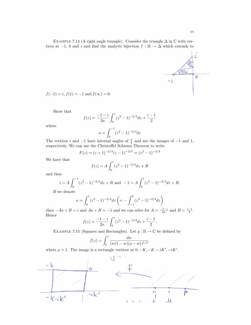
55
Example 7.14 (A right angle triangle). Consider the triangle ∆ in C with ver-tices at −1, 0 and i and find the analytic bijection f : H → ∆ which extends to
f(−1) = i, f(1) = −1 and f(∞) = 0.
Show that
f(z) =−1− i
2κ
∫ z
0
(z2 − 1)−3/4dz +i− 1
2where
κ =∫ −1
0
(z2 − 1)−3/4dz
The vertices i and −1 have internal angles of π4 and are the images of −1 and 1,
respectively, We can use the Christoffel Schwarz Theorem to write
F (z) = (z + 1)−3/4(z − 1)−3/4 = (z2 − 1)−3/4
We have that
f(z) = A
∫ z
0
(z2 − 1)−3/4dz +B
and then
i = A
∫ −1
0
(z2 − 1)−3/4dz +B and − 1 = A
∫ 1
0
(z2 − 1)−3/4dz +B.
If we denote
κ =∫ 1
0
(z2 − 1)−3/4dz
(= −
∫ 0
−1
(z2 − 1)−3/4dz
)then −Aκ+B = i and Aκ+B = −1 and we can solve for A = −1−i
2κ and B = i−12 .
Hence
f(z) =−1− i
2κ
∫ z
0
(z2 − 1)−3/4dz +i− 1
2.
Example 7.15 (Squares and Rectangles). Let g : H→ C be defined by
f(z) =∫ z
0
dw
(w(1− w)(ρ− w))1/2.
where ρ > 1. The image is a rectangle vertices at 0,−K,−K − iK ′,−iK ′.

56 3
More precisely, the internal angles are all equal to π2 . It we consider the real
axis as the boundary of H then we see that the interval [0, 1] is mapped to the side[−K, 0] where
K =∫ 1
0
dw
(w(1− w)(ρ− w))1/2.
For 1 < w < ρ there is a single imaginary root and thus the integral from[1, ρ] is purely imaginary (with negative imaginary part) and the image of [1, ρ] is[−K,−K − iK ′] where
K ′ =∫ ρ
1
1(w(w − 1)(ρ− w))1/2
dw.
Similarly, we see that the image of [ρ,∞) is [−K − iK ′,−iK ′) and the image of(−∞, 0] is (−iK ′, 0].
The upper half plane H is mapped to the square by
z = f(w) =∫
dw√w(w − 1)(w + 1)
7.4. Generalizations of the Schwarz-Christofel theorem. More gener-ally one can consider an analogous problem where we introducce holes into thepicture. Let z1, . . . , zd ∈ D be the centres of subdisks Di = B(zi, ri) = z ∈D : |z − zi| < ri where |zi|+ ri < 1. We can then associate a “multiply connectedregion” defined by M = D−∪di=1Di. When d = 1 this simply corresponds to an an-nulus. Similarly, we can consider sub-polygons P1, · · · ,Pd ⊂ P with sets of verticesV1, · · · , Vd, respectively. We then let Q = P− ∪di=1Pi
Let Ci = ∂Di and let Ci denote the images on reflection in the unit circle
z ∈ C : |z| = 1 = ∂D. In particular, gi(z) = zi + r2j z
1−zjz satisfies gi(Ci) = Ci. LetΓ = 〈g1, · · · , gd〉 be the associated Schottky group. By a result of Crowdy et al,there is an explicit formula for a holomorphic bijection ψ : D→ P given by
ψ(z) =∫ z
z0
C(·)k∏i=1
w(z, wi)αid∏i=1
|Vi|∏j=1
w(z, w(i)j )α
(j)i dz. (2)
where w(·, ·) is the Schottky-Klein prime function and
(1) the exponents α1, · · · , αk correspond to the internal angles of P and ex-ponents α(j)
1 , · · · , α(j)n|Vi|
correspond to the internal angles of P(j);(2) the points W = w1, · · · , wk ∈ ∂D on the unit circle correspond to
preimages of the vertices V and the points W (i) = w(i)1 , · · · , w(i)
|Vi| ∈ ∂Di
on the circle correspond to preimages of the vertices Vi;(3) C(·) is an explicit correction function.
7.5. Application: Fluid dynamics. The streamlines around a circular re-gion of diameter 2a can be described by transforming the horizontal lines past aslit of width 4a by the associated conformal map f(z) = z + a2/z. More gener-ally, given a finite number of disjoint circular regions the stream lines described bytransforming the horizontal lines past a slits. ??
8. Behaviour of analytic functions
There are very useful tools in complex analysis: The Maximum Principle, andthe Schwarz and Pick Lemmas

8. BEHAVIOUR OF ANALYTIC FUNCTIONS 57
8.1. The Maximum Modulus Principle. The next theorem shows that thesupremum of the modulus of an analytic function isn’t achieved inside U .
Theorem 8.1 (Maximum Modulus Principle). Let f : U → C be analytic. LetU be connected. If z0 ∈ U satisfies |f(z0)| ≥ |f(z)| for all z ∈ U then f(z) isnecessarily a constant function.
Proof. By multiplying by a constant, if necessary, we can assume without lossof generality that f(z0) ∈ R+. Let
S = z ∈ U : |f(z)| = f(z0).Since f is continuous we see that S ⊂ U is a closed set.
We claim that S ⊂ U is also open. Given z ∈ S ⊂ U , since U is open we canchoose r > 0 sufficiently small that B(z, r) ⊂ U . Then for any 0 < r′ < r we haveby Cauchy’s Theorem that
f(z0) = |f(z)| =
∣∣∣∣∣ 12πi
∫C(0,r′)
f(ξ)z − ξ
dξ
∣∣∣∣∣=∣∣∣∣ 12πi
∫ 2π
0
f(z + r′eiθ)r′eiθ
(ieiθ)dθ∣∣∣∣
=∣∣∣∣ 12πi
∫ 2π
0
f(z + r′eiθ)dθ∣∣∣∣
≤ 12π
∫ 2π
0
∣∣f(z + r′eiθ)∣∣ dθ ≤ f(z0) = |f(z)|,
where |f(z+ r′eit)| ≤ |f(z)| = f(z0), since z ∈ S. Thus all the inequalities must beequalities and so
|f(z + r′eiθ)| = f(z0)for all 0 ≤ θ < 2π and all 0 < r′ < r. In particular, S contains the open ballB(z, r) ⊂ S. But since S is both open and closed and U is connected we deducethat S = U and thus f takes the constant value f(z0).
8.2. The Schwarz Lemma. The next result describes analytic maps of thedisk D = z ∈ C : |z| < 1 to itself.
Theorem 8.2 (Schwarz Lemma). Let f : D→ D be an analytic map.(1) Let f(0) = 0 then:
(a) |f(z0)| ≤ |z0|, ∀z0 ∈ D; and(b) |f ′(0)| ≤ 1.
(2) Moreover, if either |f(z)| = |z| for some z ∈ D − 0 or |f ′(0)| = 1 thenf is a “rotation” of the form f(z) = eiθz, for some 0 ≤ θ < 2π.
Proof. (1) The function g : D→ C defined by
g(z) =
f(z)z if z 6= 0
f ′(0) if z = 0
is analytic on D. Fix ε > 0. We can apply the Maximum Modulus Principle to therestriction g : B(0, 1− ε)→ C to deduce that for |z| ≤ 1− ε we have that
|g(z)| ≤ 11− ε
.
Letting ε→ 0 we deduce that |g(z)| ≤ 1 whenever |z| ≤ 1. From the definition of gthis completes the proof of the first part.
(2) For the second part, if |f(z0)| = |z0| then |g(z0)| = 1. The maximumprinciple principle applied to g now tells us that g has a constant value, eiθ, say.This implies that f(z) is a rotation.
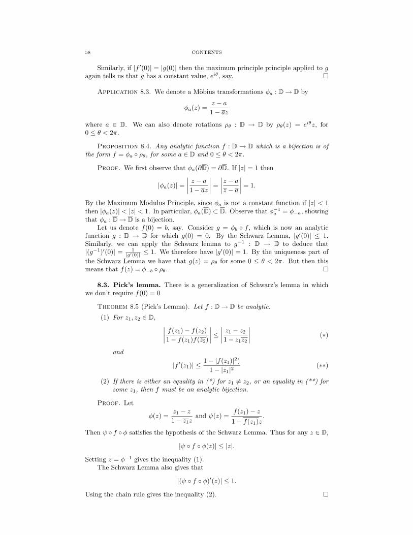
58 CONTENTS
Similarly, if |f ′(0)| = |g(0)| then the maximum principle principle applied to gagain tells us that g has a constant value, eiθ, say.
Application 8.3. We denote a Mobius transformations φa : D→ D by
φa(z) =z − a1− az
where a ∈ D. We can also denote rotations ρθ : D → D by ρθ(z) = eiθz, for0 ≤ θ < 2π.
Proposition 8.4. Any analytic function f : D → D which is a bijection is ofthe form f = φa ρθ, for some a ∈ D and 0 ≤ θ < 2π.
Proof. We first observe that φa(∂D) = ∂D. If |z| = 1 then
|φa(z)| =∣∣∣∣ z − a1− az
∣∣∣∣ =∣∣∣∣z − az − a
∣∣∣∣ = 1.
By the Maximum Modulus Principle, since φa is not a constant function if |z| < 1then |φa(z)| < |z| < 1. In particular, φa(D) ⊂ D. Observe that φ−1
a = φ−a, showingthat φa : D→ D is a bijection.
Let us denote f(0) = b, say. Consider g = φb f , which is now an analyticfunction g : D → D for which g(0) = 0. By the Schwarz Lemma, |g′(0)| ≤ 1.Similarly, we can apply the Schwarz lemma to g−1 : D → D to deduce that|(g−1)′(0)| = 1
|g′(0)| ≤ 1. We therefore have |g′(0)| = 1. By the uniqueness part ofthe Schwarz Lemma we have that g(z) = ρθ for some 0 ≤ θ < 2π. But then thismeans that f(z) = φ−b ρθ.
8.3. Pick’s lemma. There is a generalization of Schwarz’s lemma in whichwe don’t require f(0) = 0
Theorem 8.5 (Pick’s Lemma). Let f : D→ D be analytic.
(1) For z1, z2 ∈ D, ∣∣∣∣ f(z1)− f(z2)1− f(z1)f(z2)
∣∣∣∣ ≤ ∣∣∣∣ z1 − z2
1− z1z2
∣∣∣∣ (∗)
and
|f ′(z1)| ≤ 1− |f(z1)|2)1− |z1|2
(∗∗)
(2) If there is either an equality in (*) for z1 6= z2, or an equality in (**) forsome z1, then f must be an analytic bijection.
Proof. Let
φ(z) =z1 − z1− z1z
and ψ(z) =f(z1)− z1− f(z1)z
.
Then ψ f φ satisfies the hypothesis of the Schwarz Lemma. Thus for any z ∈ D,
|ψ f φ(z)| ≤ |z|.
Setting z = φ−1 gives the inequality (1).The Schwarz Lemma also gives that
|(ψ f φ)′(z)| ≤ 1.
Using the chain rule gives the inequality (2).
9. HARMONIC FUNCTIONS 59
9. Harmonic functions
We want to consider the real valued functions.
Definition 9.1. We say that any function u : U → R is harmonic if ∆u = 0where
∆ =∂2
∂x2+
∂2
∂y2
Remark 9.2. Any scaler multiple of linear combinations of harmonic functionsare harmonic.
In particular, if f : U → C is analytic and f(x+ iy) = u(x, y) + iv(x, y) satisfythe Cauchy-Riemann equations then differentiating
∂u
∂x=∂v
∂y
with respect to x implies that∂2u
∂x2=
∂2v
∂y∂x
and differentiating∂u
∂y= −∂v
∂x
with respect to y implies that
∂2u
∂y2= − ∂2v
∂y∂x.
Thus we have shown:
Theorem 9.3. We have that u = Re(f) is harmonic. Similarly, we see thatv = Im(f) is harmonic.
Example 9.4. The function f : C→ C given by f(z) = z2 is analytic and thus
f(z) = (u(x, y) + iv(x, y))
= (x+ iy)2
= x2 − y2 + 2ixy.
where u(x, y) = x2 − y2 and v(x, y) = xy are harmonic.
Example 9.5. Let f : U → C be analytic and for z = x + iy and writef(z) = u(z) + iv(z). Let w(z) := log |f(z)| = 1
2 log(u(z)2 + v(z)2) then
∂w
∂x=
1u(z)2 + v(z)2
(u(z)
∂u
∂x+ v(z)
∂v
∂x
)∂w
∂y=
1u(z)2 + v(z)2
(u(z)
∂u
∂y+ v(z)
∂v
∂y
)and
∂2w
∂x2=
−2(u(z)2 + v(z)2)2
(u(z)
∂u
∂x+ v(z)
∂v
∂x
)2
+1
u(z)2 + v(z)2
((∂u
∂x
)2
+(∂v
∂x
)2
+ u(z)∂2u
∂x2+ v(z)
∂2v
∂x2
)∂2w
∂y2=
−2(u(z)2 + v(z)2)2
(u(z)
∂u
∂y+ v(z)
∂v
∂y
)2
+1
u(z)2 + v(z)2
((∂u
∂y
)2
+(∂v
∂y
)2
+ u(z)∂2u
∂y2+ v(z)
∂2v
∂y2
)Adding these, expressions, the second derivative terms vanish since u and v areharmonic. The first order terms vanish by the Cauchy-Riemann equations.
Remark 9.6. The equation ∆u = 0 is called Laplace’s equation.
60 CONTENTS
9.1. Harmonic conjugates.
Definition 9.7. If u, v are harmonic and satisfy the Cauchy-Riemann equa-tions in u then v is called the harmonic conjugate of u.
Conversely, if u is harmonic then it is the real part of an analytic function.
Theorem 9.8. If u : U → R is a C2 function there there exists a harmonicconjugate, i.e., there exists a C2 function v : U → R such that the function f : U →C defined by f = u+ iv is analytic.
Proof. Consider the case
U = z = x+ iy : x ∈ (a− δ, a+ δ) and y ∈ (b− ε, b+ ε),and let f, g : U → R be C1 functions defined by
f(z) = −∂u(z)∂y
and g(z) =∂u(z)∂x
.
Then since ∆u = 0 we have that∂f
∂y=∂g
∂x
(= −∂
2u
∂y2=∂2v
∂x2
). (1)
If we define
v(x, y) =∫ x
a
f(t, b)dt+∫ y
b
g(x, s)ds (2)
then v : U → R is a C2 function such that ∂h∂y = g. The derivative with respect to
x is a little more complicated. We can write∂
∂x
∫ x
a
f(t, b)dt = f(x, b). (3)
For the second term in (2) we have that∂
∂x
∫ y
b
g(x, s)ds =∫ y
b
∂g
∂x(x, s)︸ ︷︷ ︸
= ∂f∂y by (1)
ds =∫ y
b
∂f
∂y(x, s)ds = f(x, y)− f(x, b).
(4)
Comparing (2), (3) and (4) gives that∂v
∂x= f = f(x, b) + (f(x, y)− f(x, b)) = f(x, y).
Finally, ∂u∂x = g = ∂v∂y and ∂u
∂y = −f = ∂v∂x .
Exercise 9.9. Given u(x, y) = xy find the harmonic conjugate of u. In par-ticular,
∂u
∂x= y =
∂v
∂y=⇒ v(x, y) =
12y2 + f(x)
∂v
∂x= f ′(x) = −∂u
∂y= x =⇒ f(x) = −1
2x2 + C
Therefore v(x, y) = 12 (−x2 + y2) + C and
f(z) = u+ iv
= xy + i(−x2 + y2)
2+ C
= − i2
(x+ iy)2 + C
= − i2z2 + C.
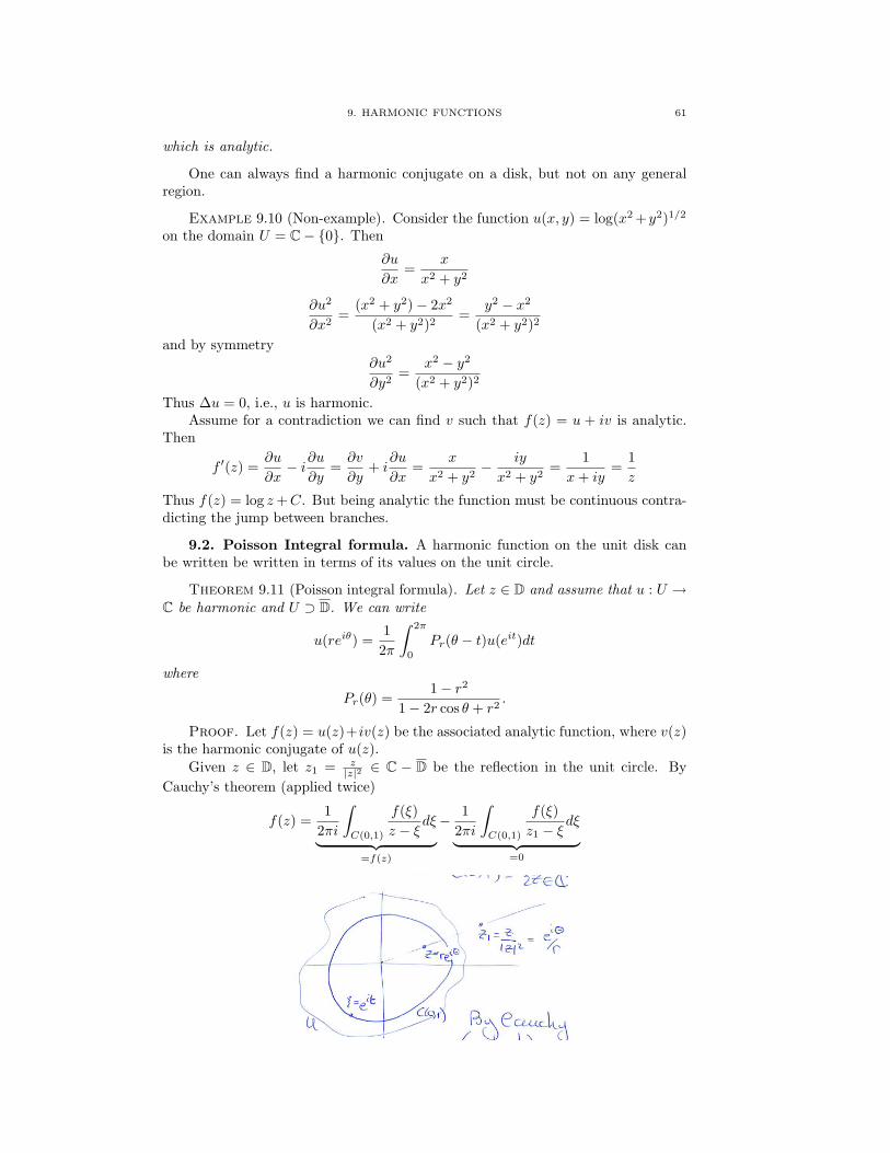
9. HARMONIC FUNCTIONS 61
which is analytic.
One can always find a harmonic conjugate on a disk, but not on any generalregion.
Example 9.10 (Non-example). Consider the function u(x, y) = log(x2 +y2)1/2
on the domain U = C− 0. Then
∂u
∂x=
x
x2 + y2
∂u2
∂x2=
(x2 + y2)− 2x2
(x2 + y2)2=
y2 − x2
(x2 + y2)2
and by symmetry∂u2
∂y2=
x2 − y2
(x2 + y2)2
Thus ∆u = 0, i.e., u is harmonic.Assume for a contradiction we can find v such that f(z) = u + iv is analytic.
Then
f ′(z) =∂u
∂x− i∂u
∂y=∂v
∂y+ i
∂u
∂x=
x
x2 + y2− iy
x2 + y2=
1x+ iy
=1z
Thus f(z) = log z+C. But being analytic the function must be continuous contra-dicting the jump between branches.
9.2. Poisson Integral formula. A harmonic function on the unit disk canbe written be written in terms of its values on the unit circle.
Theorem 9.11 (Poisson integral formula). Let z ∈ D and assume that u : U →C be harmonic and U ⊃ D. We can write
u(reiθ) =1
2π
∫ 2π
0
Pr(θ − t)u(eit)dt
where
Pr(θ) =1− r2
1− 2r cos θ + r2.
Proof. Let f(z) = u(z)+iv(z) be the associated analytic function, where v(z)is the harmonic conjugate of u(z).
Given z ∈ D, let z1 = z|z|2 ∈ C − D be the reflection in the unit circle. By
Cauchy’s theorem (applied twice)
f(z) =1
2πi
∫C(0,1)
f(ξ)z − ξ
dξ︸ ︷︷ ︸=f(z)
− 12πi
∫C(0,1)
f(ξ)z1 − ξ
dξ︸ ︷︷ ︸=0
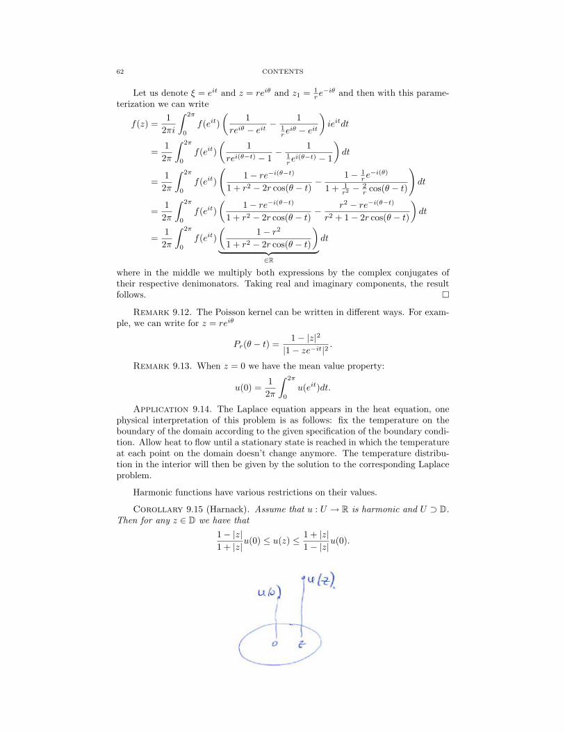
62 CONTENTS
Let us denote ξ = eit and z = reiθ and z1 = 1r e−iθ and then with this parame-
terization we can write
f(z) =1
2πi
∫ 2π
0
f(eit)(
1reiθ − eit
− 11r eiθ − eit
)ieitdt
=1
2π
∫ 2π
0
f(eit)(
1rei(θ−t) − 1
− 11r ei(θ−t) − 1
)dt
=1
2π
∫ 2π
0
f(eit)
(1− re−i(θ−t)
1 + r2 − 2r cos(θ − t)−
1− 1r e−i(θ)
1 + 1r2 −
2r cos(θ − t)
)dt
=1
2π
∫ 2π
0
f(eit)(
1− re−i(θ−t)
1 + r2 − 2r cos(θ − t)− r2 − re−i(θ−t)
r2 + 1− 2r cos(θ − t)
)dt
=1
2π
∫ 2π
0
f(eit)(
1− r2
1 + r2 − 2r cos(θ − t)
)︸ ︷︷ ︸
∈R
dt
where in the middle we multiply both expressions by the complex conjugates oftheir respective denimonators. Taking real and imaginary components, the resultfollows.
Remark 9.12. The Poisson kernel can be written in different ways. For exam-ple, we can write for z = reiθ
Pr(θ − t) =1− |z|2
|1− ze−it|2.
Remark 9.13. When z = 0 we have the mean value property:
u(0) =1
2π
∫ 2π
0
u(eit)dt.
Application 9.14. The Laplace equation appears in the heat equation, onephysical interpretation of this problem is as follows: fix the temperature on theboundary of the domain according to the given specification of the boundary condi-tion. Allow heat to flow until a stationary state is reached in which the temperatureat each point on the domain doesn’t change anymore. The temperature distribu-tion in the interior will then be given by the solution to the corresponding Laplaceproblem.
Harmonic functions have various restrictions on their values.
Corollary 9.15 (Harnack). Assume that u : U → R is harmonic and U ⊃ D.Then for any z ∈ D we have that
1− |z|1 + |z|
u(0) ≤ u(z) ≤ 1 + |z|1− |z|
u(0).
9. HARMONIC FUNCTIONS 63
Proof. We observe that for any 0 ≤ t < 2π and z ∈ D:
1− |z|2
|eit − z|2≤ 1− |z|2
(1− |z|)2=
1 + |z|1− |z|
.
Thus by the Poisson Integral Theorem
u(z) ≤ 1 + |z|1− |z|
12π
∫ 2π
0
u(eit)dt =1 + |z|1− |z|
u(0).
The other inequality is proved similarly.
The following is the analogue of Montel’s theorem for analytic functions.
Corollary 9.16 (Harnack’s Principle). Assume that uj : U → R, j ≥ 1, areharmonic functions with
u1 ≤ u2 ≤ u3 ≤ · · ·Then either uj → ∞ uniformly on compacts sets or there is a harmonic functionu : U → R such that uj → u uniformly on compact sets.
This is an exercise.
Corollary 9.17 (Jensen). Let f : U → R be analytic and let U ⊃ D. Leta1, · · · , aN ∈ D be the zeros of f(z) with |aj | < 1, for j = 1, · · · , N , and assumethere are no zeros on C(0, 1). Then
log |f(0)| =N∑j=1
log |aj |+1
2π
∫ 2π
0
log |f(eit)|dt
Proof. If f(z) has no zeros then u(z) := log |f(z)| is harmonic and by thePoisson Integral Formula (at z = 0) we have that
log |f(0)| = 12π
∫ 2π
0
log |f(eit)|dt. (1)
More generally, if f(z) has zeros a1, · · · , aN ∈ D then we can define
F (z) :=
N∏j=1
1− zajz − aj
f(z)
which is now a zero free analytic function. We can apply (1) to F (z) to deduce that
log |F (0)| = log |f(0)|+N∑i=1
log∣∣∣∣ 1ai
∣∣∣∣=
12π
∫ 2π
0
log |F (eit)|dt
=1
2π
∫ 2π
0
log |f(eit)|+N∑i=1
log∣∣∣∣1− aieiteit − aj
∣∣∣∣︸ ︷︷ ︸=1
dt
=1
2π
∫ 2π
0
log |f(eit)|dt
since the maps z 7→ 1−zaiz−ai preserve the unit circles.
Application 9.18 (The Dirichlet problem). We can construct harmonic func-tions on D from a continuous function on the unit circle.
64 CONTENTS
Theorem 9.19. Let U : C(0, 1)→ R be continuous on the boundary of the unitdisk D. Then the function u : D→ R defined by
u(z) =
U(z) if z ∈ C(0, 1)1
2π
∫ 2π
0Pr(θ − t)f(eit)dt if z = reiθ ∈ D
is harmonic (i.e., ∆u = 0)
Proof. We can rewrite
Pr(θ − t) =1− |z|2
|z − eit|2=
eit
eit − z+
e−it
e−it − z− 1
where z = reiθ. Then
u(z) =1
2π
∫ 2π
0
Pr(θ − t)U(eit)dt
=1
2π
∫ 2π
0
(eit
eit − z+
e−it
e−it − z− 1)U(eit)dt.
For the first integral we have observe that
∂2
∂x2
∫ 2π
0
(eit
eit − (x+ iy)
)U(eit)dt =
∫ 2π
0
(−2eit
(eit − (x+ iy))3
)U(eit)dt
and∂2
∂y2
∫ 2π
0
(eit
eit − (x+ iy)
)U(eit)dt =
∫ 2π
0
(2eit
(eit − (x+ iy))3
)U(eit)dt
and thus adding these two expressions gives
∆∫ (
eit
eit − (x+ iy)
)U(eit)dt = 0.
The second integral is similarly. The final term is a constant. Thus three terms areharmonic, and thus so is the sum.
To see that u(z) is continuous (on the boundary) we can write
12π
∫ 2π
0
Pr(θ − t)U(eit)dt =1
2π
∫ 2π
0
(1− |z|2
|z − eit|
)U(eit)dt
=1
2π
∫ 2π
0
U
(eit + z
1 + zeit
)dt
using the change of variables φ−z(w) = w+z1+zw (with |φ′−z(w)| = 1−|z|2
|1+zw|2 ) for eachz ∈ D. Moreover, since for each ξ ∈ C(0, 1) we have
limz→ξ
(eit + z
1 + zeit
)= ξ
if ξ 6= −eit. The result follows from bounded convergence of integrals.
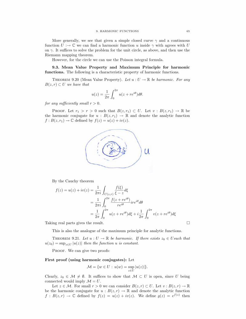
9. HARMONIC FUNCTIONS 65
More generally, we see that given a simple closed curve γ and a continuousfunction U :→ C we can find a harmonic function u inside γ with agrees with Uon γ. It suffices to solve the problem for the unit circle, as above, and then use theRiemann mapping theorem.
However, for the circle we can use the Poisson integral formula.
9.3. Mean Value Property and Maximum Principle for harmonicfunctions. The following is a characteristic property of harmonic functions.
Theorem 9.20 (Mean Value Property). Let u : U → R be harmonic. For anyB(z, r) ⊂ U we have that
u(z) =1
2π
∫ 2π
0
u(z + reiθ)dθ.
for any sufficiently small r > 0.
Proof. Let r1 > r > 0 such that B(z, r1) ⊂ U . Let v : B(z, r1) → R bethe harmonic conjugate for u : B(z, r1) → R and denote the analytic functionf : B(z, r1)→ C defined by f(z) = u(z) + iv(z).
By the Cauchy theorem
f(z) = u(z) + iv(z) =1
2πi
∫C(z,r)
f(ξ)ξ − z
dξ
=1
2πi
∫ 2π
0
f(z + reiθ)reiθ
ireiθdθ
=1
2π
∫ 2π
0
u(z + reiθ)dξ + i1
2π
∫ 2π
0
v(z + reiθ)dξ
Taking real parts gives the result.
This is also the analogue of the maximum principle for analytic functions.
Theorem 9.21. Let u : U → R be harmonic. If there exists z0 ∈ Usuch thatu(z0) = supz∈U |u(z)| then the function u is constant.
Proof. We can give two proofs:
First proof (using harmonic conjugates): Let
M = w ∈ U : u(w) = supz∈U|u(z)|.
Clearly, z0 ∈ M 6= ∅. It suffices to show that M ⊂ U is open, since U beingconnected would imply M = U .
Let z ∈ M. For small r > 0 we can consider B(z, r) ⊂ U . Let v : B(z, r)→ Rbe the harmonic conjugate for u : B(z, r) → R and denote the analytic functionf : B(z, r) → C defined by f(z) = u(z) + iv(z). We define g(z) = ef(z) then
66 CONTENTS
|g(z)| = supξ∈B(z,r) |g(ξ)|. We can apply the maximum modulus principle for ana-lytic functions to deduce that g(z) is constant on B(z, r), and thus u(z) = log |g(z)|is constant on B(z, r). Thus M is open.
Second proof (using mean value property): Let L := supz∈U |u(z)| and let
M = w ∈ U : u(w) = L.By hypothesis z0 ∈ M 6= ∅. Since g is continuous we see that M is closed. Itsuffices to show it is also open.
Let z ∈M and choose r > 0 such that B(z, r) ⊂ U and then
L = g(z) =1
2π
∫ 2π
0
g(z + reiθ)dθ ≤ L
and thus g(z+ reiθ) = L for 0 ≤ θ < 2π, for all sufficiently small r > 0. We deducethat M is open.
We can use this to get the converse to the first result.
Theorem 9.22. If h : U → R satisfies the mean value theorem then it isharmonic.
Proof. Assume that B(z, r) ⊂ U . By using the Poisson Integral Theorem wehave a harmonic function u : B(z, r)→ R which coincides with h on the boundaryC(z0, r). It suffices to show that u and h therefore coincide on all of B(z, r).
Let us write g(z) = u(z) − h(z), which vanishes on C(z0, r). Moreover, itsatisfies the mean value theorem since this holds for both u (since it is harmonic)and h (by hypothesis). By the previous lemma we see that g ≤ 0 (since otherwisethe supremum would occur in B(z, r) and this would make the function constant,giving a contradiction). Replacing w by −w we deduce that w = 0, i.e., u(z) = h(z)on B(z, r). Since the disk is arbitrary we deduce that h(z) is analytic on U .
9.4. Schwarz reflection principle for harmonic functions. We can nowformulate an analogue of the Schwarz reflection principle for functions.
Theorem 9.23. Given a domain U and suppose that U ∩ R = (a, b). LetU+ = z ∈ U : Im(z) > 0. Assume v : U+ → R is harmonic and for eachz0 ∈ (a, b) we have that limz→z0 v(z) = 0. Let U− = z : z ∈ U and define
w(z) =
v(z) if z ∈ U+
0 if z ∈ (a, b)−v(z) if z ∈ U−
Then w : U+ ∪ (a, b) ∪ U− → R is harmonic.
Proof. We claim that the Mean Value Theorem holds on a sufficiently smalldisk about any point. If z ∈ U+ then it follows form u being harmonic. Similarly,it holds for z ∈ U−.
If z ∈ (a, b) then for sufficiently small r > 0 we have that
12π
∫ 2π
0
w(z + reiθ)dθ
=1
2π
∫ π
0
w(z + reiθ)dθ +1
2π
∫ π
0
w(z + reiθ+iπ)dθ
=1
2π
∫ π
0
w(z + reiθ)dθ +1
2π
∫ π
0
w(z − reiθ)dθ
=1
2π
∫ π
0
w(z + reiθ)dθ − 12π
∫ π
0
w(z + reiθ)dθ = 0.
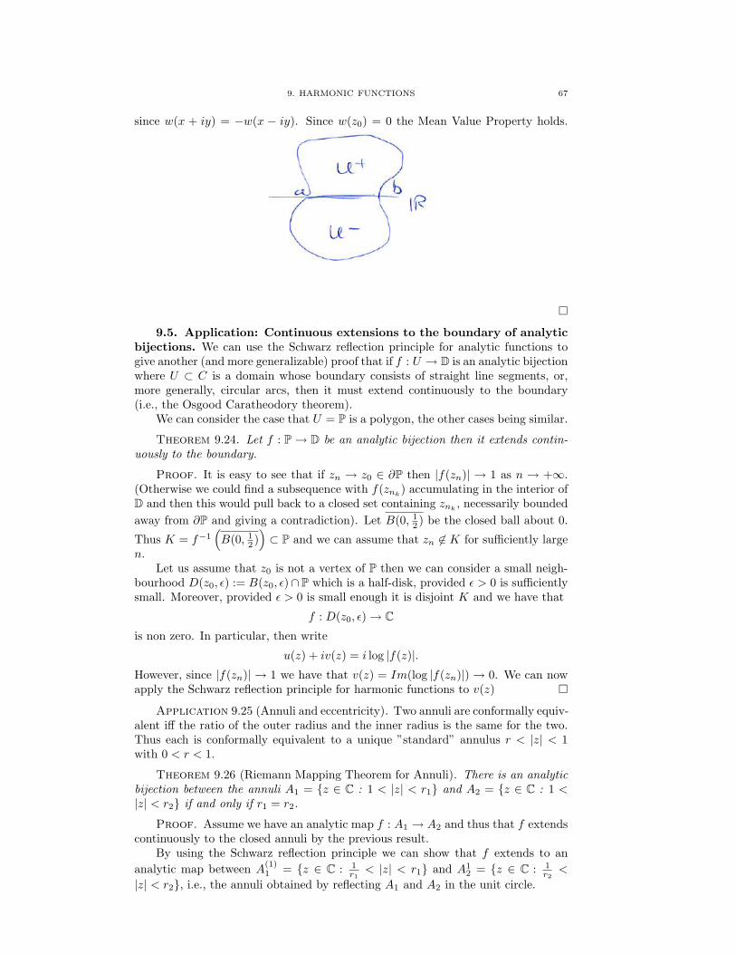
9. HARMONIC FUNCTIONS 67
since w(x + iy) = −w(x − iy). Since w(z0) = 0 the Mean Value Property holds.
9.5. Application: Continuous extensions to the boundary of analyticbijections. We can use the Schwarz reflection principle for analytic functions togive another (and more generalizable) proof that if f : U → D is an analytic bijectionwhere U ⊂ C is a domain whose boundary consists of straight line segments, or,more generally, circular arcs, then it must extend continuously to the boundary(i.e., the Osgood Caratheodory theorem).
We can consider the case that U = P is a polygon, the other cases being similar.
Theorem 9.24. Let f : P→ D be an analytic bijection then it extends contin-uously to the boundary.
Proof. It is easy to see that if zn → z0 ∈ ∂P then |f(zn)| → 1 as n → +∞.(Otherwise we could find a subsequence with f(znk) accumulating in the interior ofD and then this would pull back to a closed set containing znk , necessarily boundedaway from ∂P and giving a contradiction). Let B(0, 1
2 ) be the closed ball about 0.
Thus K = f−1(B(0, 1
2 ))⊂ P and we can assume that zn 6∈ K for sufficiently large
n.Let us assume that z0 is not a vertex of P then we can consider a small neigh-
bourhood D(z0, ε) := B(z0, ε)∩ P which is a half-disk, provided ε > 0 is sufficientlysmall. Moreover, provided ε > 0 is small enough it is disjoint K and we have that
f : D(z0, ε)→ Cis non zero. In particular, then write
u(z) + iv(z) = i log |f(z)|.However, since |f(zn)| → 1 we have that v(z) = Im(log |f(zn)|) → 0. We can nowapply the Schwarz reflection principle for harmonic functions to v(z)
Application 9.25 (Annuli and eccentricity). Two annuli are conformally equiv-alent iff the ratio of the outer radius and the inner radius is the same for the two.Thus each is conformally equivalent to a unique ”standard” annulus r < |z| < 1with 0 < r < 1.
Theorem 9.26 (Riemann Mapping Theorem for Annuli). There is an analyticbijection between the annuli A1 = z ∈ C : 1 < |z| < r1 and A2 = z ∈ C : 1 <|z| < r2 if and only if r1 = r2.
Proof. Assume we have an analytic map f : A1 → A2 and thus that f extendscontinuously to the closed annuli by the previous result.
By using the Schwarz reflection principle we can show that f extends to ananalytic map between A
(1)1 = z ∈ C : 1
r1< |z| < r1 and A1
2 = z ∈ C : 1r2<
|z| < r2, i.e., the annuli obtained by reflecting A1 and A2 in the unit circle.
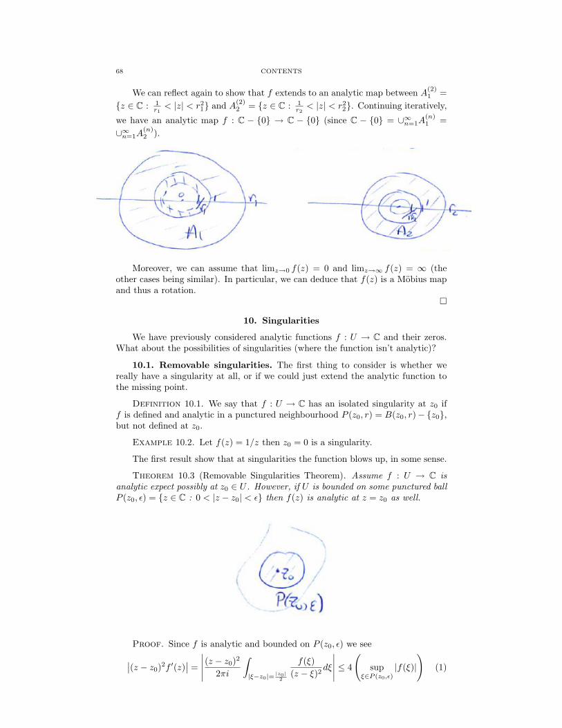
68 CONTENTS
We can reflect again to show that f extends to an analytic map between A(2)1 =
z ∈ C : 1r1< |z| < r2
1 and A(2)2 = z ∈ C : 1
r2< |z| < r2
2. Continuing iteratively,
we have an analytic map f : C − 0 → C − 0 (since C − 0 = ∪∞n=1A(n)1 =
∪∞n=1A(n)2 ).
Moreover, we can assume that limz→0 f(z) = 0 and limz→∞ f(z) = ∞ (theother cases being similar). In particular, we can deduce that f(z) is a Mobius mapand thus a rotation.
10. Singularities
We have previously considered analytic functions f : U → C and their zeros.What about the possibilities of singularities (where the function isn’t analytic)?
10.1. Removable singularities. The first thing to consider is whether wereally have a singularity at all, or if we could just extend the analytic function tothe missing point.
Definition 10.1. We say that f : U → C has an isolated singularity at z0 iff is defined and analytic in a punctured neighbourhood P (z0, r) = B(z0, r)− z0,but not defined at z0.
Example 10.2. Let f(z) = 1/z then z0 = 0 is a singularity.
The first result show that at singularities the function blows up, in some sense.
Theorem 10.3 (Removable Singularities Theorem). Assume f : U → C isanalytic expect possibly at z0 ∈ U . However, if U is bounded on some punctured ballP (z0, ε) = z ∈ C : 0 < |z − z0| < ε then f(z) is analytic at z = z0 as well.
Proof. Since f is analytic and bounded on P (z0, ε) we see∣∣(z − z0)2f ′(z)∣∣ =
∣∣∣∣∣ (z − z0)2
2πi
∫|ξ−z0|= |z0|2
f(ξ)(z − ξ)2
dξ
∣∣∣∣∣ ≤ 4
(sup
ξ∈P (z0,ε)
|f(ξ)|
)(1)
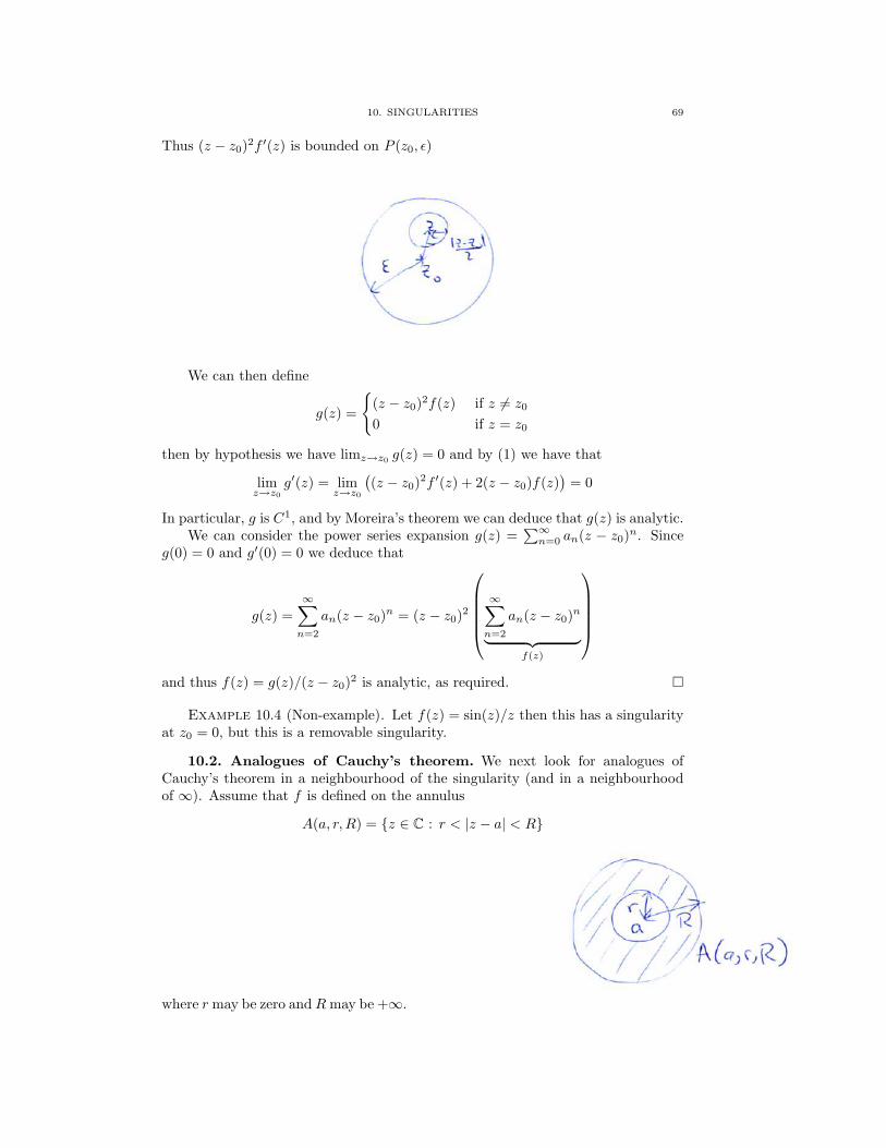
10. SINGULARITIES 69
Thus (z − z0)2f ′(z) is bounded on P (z0, ε)
We can then define
g(z) =
(z − z0)2f(z) if z 6= z0
0 if z = z0
then by hypothesis we have limz→z0 g(z) = 0 and by (1) we have that
limz→z0
g′(z) = limz→z0
((z − z0)2f ′(z) + 2(z − z0)f(z)
)= 0
In particular, g is C1, and by Moreira’s theorem we can deduce that g(z) is analytic.We can consider the power series expansion g(z) =
∑∞n=0 an(z − z0)n. Since
g(0) = 0 and g′(0) = 0 we deduce that
g(z) =∞∑n=2
an(z − z0)n = (z − z0)2
∞∑n=2
an(z − z0)n︸ ︷︷ ︸f(z)
and thus f(z) = g(z)/(z − z0)2 is analytic, as required.
Example 10.4 (Non-example). Let f(z) = sin(z)/z then this has a singularityat z0 = 0, but this is a removable singularity.
10.2. Analogues of Cauchy’s theorem. We next look for analogues ofCauchy’s theorem in a neighbourhood of the singularity (and in a neighbourhoodof ∞). Assume that f is defined on the annulus
A(a, r,R) = z ∈ C : r < |z − a| < R
where r may be zero andRmay be +∞.
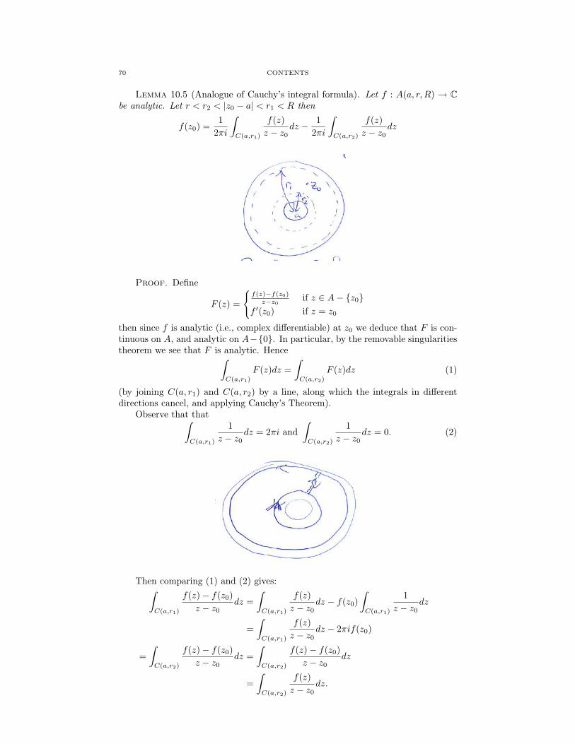
70 CONTENTS
Lemma 10.5 (Analogue of Cauchy’s integral formula). Let f : A(a, r,R) → Cbe analytic. Let r < r2 < |z0 − a| < r1 < R then
f(z0) =1
2πi
∫C(a,r1)
f(z)z − z0
dz − 12πi
∫C(a,r2)
f(z)z − z0
dz
Proof. Define
F (z) =
f(z)−f(z0)
z−z0 if z ∈ A− z0f ′(z0) if z = z0
then since f is analytic (i.e., complex differentiable) at z0 we deduce that F is con-tinuous on A, and analytic on A−0. In particular, by the removable singularitiestheorem we see that F is analytic. Hence∫
C(a,r1)
F (z)dz =∫C(a,r2)
F (z)dz (1)
(by joining C(a, r1) and C(a, r2) by a line, along which the integrals in differentdirections cancel, and applying Cauchy’s Theorem).
Observe that that∫C(a,r1)
1z − z0
dz = 2πi and∫C(a,r2)
1z − z0
dz = 0. (2)
Then comparing (1) and (2) gives:∫C(a,r1)
f(z)− f(z0)z − z0
dz =∫C(a,r1)
f(z)z − z0
dz − f(z0)∫C(a,r1)
1z − z0
dz
=∫C(a,r1)
f(z)z − z0
dz − 2πif(z0)
=∫C(a,r2)
f(z)− f(z0)z − z0
dz =∫C(a,r2)
f(z)− f(z0)z − z0
dz
=∫C(a,r2)
f(z)z − z0
dz.
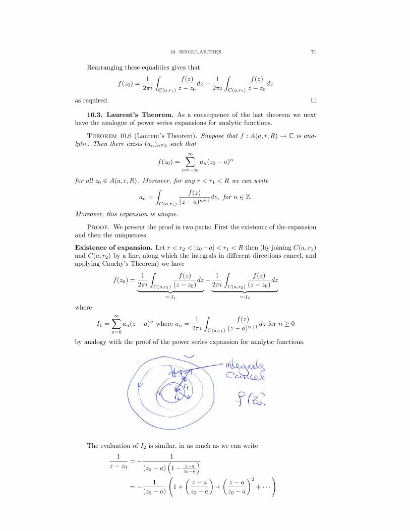
10. SINGULARITIES 71
Rearranging these equalities gives that
f(z0) =1
2πi
∫C(a,r1)
f(z)z − z0
dz − 12πi
∫C(a,r2)
f(z)z − z0
dz
as required.
10.3. Laurent’s Theorem. As a consequence of the last theorem we nexthave the analogue of power series expansions for analytic functions.
Theorem 10.6 (Laurent’s Theorem). Suppose that f : A(a, r,R) → C is ana-lytic. Then there exists (an)n∈Z such that
f(z0) =∞∑
n=−∞an(z0 − a)n
for all z0 ∈ A(a, r, R). Moreover, for any r < r1 < R we can write
an =∫C(a,r1)
f(z)(z − a)n+1
dz, for n ∈ Z.
Moreover, this expansion is unique.
Proof. We present the proof in two parts: First the existence of the expansionand then the uniqueness.
Existence of expansion. Let r < r2 < |z0−a| < r1 < R then (by joining C(a, r1)and C(a, r2) by a line, along which the integrals in different directions cancel, andapplying Cauchy’s Theorem) we have
f(z0) =1
2πi
∫C(a,r1)
f(z)(z − z0)
dz︸ ︷︷ ︸=:I1
− 12πi
∫C(a,r2)
f(z)(z − z0)
dz︸ ︷︷ ︸=:I2
where
I1 =∞∑n=0
an(z − a)n where an =1
2πi
∫C(a,r1)
f(z)(z − a)n+1
dz for n ≥ 0
by analogy with the proof of the power series expansion for analytic functions.
The evaluation of I2 is similar, in as much as we can write
1z − z0
= − 1
(z0 − a)(
1− z−az0−a
)= − 1
(z0 − a)
(1 +
(z − az0 − a
)+(z − az0 − a
)2
+ · · ·
)
72 CONTENTS
for |z − a| = r2 < |z0 − a|. Thus
I2 =1
2πi
∫C(a,r2)
f(z)(z − z0)
dz =∞∑n=1
a−n(z0 − a)−n
where
a−n =1
2πi
∫C(a,r2)
f(z)(z − a)n−1dz =1
2πi
∫C(a,r1)
f(z)(z − a)n−1dz
since (z−a)n−1f(z) is analytic, which is justified by by the the uniform convergenceof the geometric series and integration. Hence
f(z0) = I1 − I2 =∞∑
n=−∞an(z0 − a)n
where an is as given. 1
Uniqueness of expansion. To see the uniqueness of the coefficients, supposef(z) =
∑∞n=−∞ bn(z − a)n then dividing by (z − a)k+1 and integrating around a
circle C with radius between r and R, i.e.,
12πi
∫C
f(z)(z − a)k+1
dz =∞∑
n=−∞bn
(1
2πi
∫C
(z − a)n−k−1dz
)= bk
showing uniqueness.
Example 10.7. We can consider the function
f(z) =1
(z − 1)(z − 2)=
1(z − 2)
− 1(z − 1)
on various domains. Observe that we can expand
1z − 1
=
−∑∞n=0 z
n if |z| < 1∑∞n=1 z
−n if |z| > 1
and1
z − 2=
−∑∞n=0 2−n−1zn if |z| < 2∑∞
n=1 2n−1z−n if |z| > 2.
Case I: For z ∈ D(0, 1) we have an expansion
f(z) = −∞∑n=0
(1− 2−n−1)zn.
This is a power series which is analytic (and with no negative powers involved),
Case II: For z ∈ A(0, 1, 2) we have a Laurent series expansion
f(z) =∞∑n=0
z−n −∞∑n=0
2−n−1zn.
Case III: For z ∈ A(0, 2,∞) (i.e., |z| > 2) we have a Laurent series expansion
f(z) =∞∑n=0
z−n −∞∑n=0
(2n−1 − 1)zn
This brings us to the following estimate.
1The integrals around C(a, r1) and C(a, r2) can now be replaced by integrals around any
circle of radius between r and R (by connecting the circles C(a, r1) and C(a, r2) by line segmentsand integrating in both directions (so that these integrals will cancel).

10. SINGULARITIES 73
Corollary 10.8. Let f : A(0, r, R)→ C be analytic and have a Laurent series
f(z) =∞∑
n=−∞an(z − a)n
then for any r < r1 < R we can bound |an| ≤ M(r1)rn1
where M(r) = sup|z−a|=r1 |f(z)|.
Proof. Since
an =1
2πi
∫C(a,r1)
f(z)(z − a)n+1
dz
we have that
|an| ≤2πr2π
M(r)rn+11
=M(r1)rn1
.
10.4. Classification of singularities. We can now classify the different typesof singularities. Consider f : P (a,R)→ C be analytic in a punctured disk P (a,R)centred at a singularity a and let
f(z) =∞∑
n=−∞an(z − a)n
be its Laurent series on a punctured disk P (a,R) = A(a, 0, R) (where R > 0).
Definition 10.9. If a−n 6= 0 for infinitely many positive n then a is calledan essential singularity. If a−n = 0 for only many positive n then a and the leastinteger −n such that a−n 6= 0 is negative then a is called a pole of order n. In theparticular case that a−1 6= 0 and ak = 0 for k ≤ −2 we call a a simple pole.
Remark 10.10. If the least integer n such that an 6= 0 is non-negative is non-negative then a is called a removable singularity for in this case
f(z) = an(z − a)n + an+1(z − a)n+1 + · · ·
for 0 < |z − a| < R and n ≥ 0. There fore we can define (or extend) f to a by
f(a) = limz→a
=
0 if n > 0a0 if n = 0
And with this value we can define f : D(a,R) → C and it is analytic. We shallalways adopt the convention of removing singularities, in the future.
Example 10.11. Let f(z) = sin(z)/z = 1 − z2/3! + z4/5! − · · · then we canremove the singularity at z = 0 by setting f(0) = 1.
Definition 10.12. If the least n such that that an is strictly positive then f(z)is said to have a zero at a of order n.
The order of a function at a is defined by
Ord(f, a) =
−∞ if a is an essential singularity−n > 0 if a is a pole of order n0 if a is a removable singularity and f(a) 6= 0n if a is a zero of order n
Definition 10.13. A function is said to be meromorphic if it is analytic in adomain U except at a set of points which are poles (with no essential singularity).

74 CONTENTS
10.5. Behaviour at singularities. We can consider the behaviour of a func-tion near a zero or pole
Theorem 10.14. Ord(f, a) = n where n is finite if and only if ∃α, β, δ > 0 suchthat
α|z − a|n ≤ |f(z)| ≤ β|z − a|n
whenever 0 < |z − a| < δ
Proof. Assume that Ord(f, a) = n, then we can write
f(z) = an(z − a)n + an+1(z − a)n+1 + · · · = (an + g(z))(z − a)n
where an 6= 0. Moreover, g(z)→ 0 as z 7→ a and thus given 0 < ε < 1 we can write|g(z)| < ε|an| provided |z − a| < δ, provided δ is small enough. In particular, wecan write
f(z)(z − a)−n = an + g(z).and thus
|an|(1− ε) ≤ |f(z)(z − a)−n| ≤ |an|(1 + ε)if δ is small enough, giving the required bound.
Conversely, suppose
α|z − a|n ≤ |f(z)| ≤ β|z − a|n
when |z − a| is small enough then f(z)(z − a)−n is bounded in a punctured neigh-bourhood of a and hence a is a removable singularity. In particular,
f(z)(z − a)−n = an + an+1(z − a) + an+2(z − a)2 + · · ·in a punctured neighbourhood P (a, δ) of a (since f(z)(z − a)−n is analytic at a bythe removable singularity). We want to show that an 6= 0. But from the left handinequality |f(z)(z − a)−n| is bounded below since α > 0, which would not be thecase where an is equal to zero. Hence an 6= 0 and Ord(f, a) = n.
The previous result gives a rough idea of the behaviour of f near a pole (whenn is negative). The next result describes the behaviour near an essential singularity(i.e., f(P (a, δ)) ⊂ C is dense).
Theorem 10.15 (Casorati-Weierstrass). Let f have an essential singularity ata. Then for any b ∈ C and every ε, δ > 0 there exists z such that 0 < |z − a| < δsuch that |f(z)− b| < ε.
Proof. Assume for a contradiction that there exist b, ε, δ such that for all zsuch that 0 < |z − a| < δ and |f(z)− b| ≥ ε. Consider the function g : P (a, δ)→ Cdefined by
g(z) =1
f(z)− b, (1)
which, by assumption, is bounded by 1/ε in P (a, δ). Then g has a removablesingularity at a (and thus is bounded). In particular, we can write
g(z) = an(z − a)n + an+1(z − a)n+1 + · · ·where an 6= 0 and thus
g(z) = (z − a)nh(z) (2)for an analytic function h : B(a, δ) → C with h(a) 6= 0. Thus comparing (1) and(2) gives
f(z)− b =1
(z − a)nh(z). (3)
Moreover, 1/h(z) is analytic in a neighbourhood of a (since h does not vanish in aneighbourhood of a by continuity and the fact h(a) 6= 0). But (3) shows that f hasa pole at a of order n, contradicting the hypothesis of an essential singularity.
10. SINGULARITIES 75
Remark 10.16 (Picard’s Big Theorem). The following is am improvement onthe WeierstrassCasorati theorem.
Theorem 10.17 (Picard’s Big Theorem). If an analytic function f(z) has anessential singularity at a, then on any punctured disk B(a, δ the function f(z) takeson all possible complex values, with at most a single exception, infinitely often.
.
1. Show that the following series define a meromorphic function on C and determinethe set of poles and their orders
(1)∑∞n=0
(−1)n
n!(n+z)
(2)∑∞n=0
1z2+n2
(3)∑∞n=0
1(n+z)2
(4) 1z +
∑n∈Z−0
(1
z−n + 1n
)(5)
∑∞n=0
(−1)n
n!(n+z)
2. Show that
f(z) =∞∑n=1
z2
n2z2 + 8
is defined and continuous for the real values of z. Determine the region of hecomplex plane in which this function is analytic. Determine its poles.
3. Let f : C → C be a non-constant entire function. Show that the image of f isdense in C.
4. Show that the order of a pole is invariant under analytic bijections (i.e., iff : U → C has a pole at z0 of order n and φ : V → U is an analytic bijection withφ(w) = z then w is a pole for f φ : V → C of order n.
5. Let f : C → C be a meromorphic function with lim|z|→+∞ |f(z)| = ∞. Provethat f(z) is a rational function (i.e., the ratio of two polynomials).
6. Show that the Laurent series of a function on an annulus can be differentiatedterm by term to give the derivative of the function on the annulus.
7. Find the Laurent series for the following functions:(1) z/(z + 2) for |z| > 2,(2) sin(1/z) for z 6= 0,(3) cos(1/z) for z 6= 0,(4) 1/(z − 3) for |z| > 3.
8. Prove the following expansions:(1) ez = e+ e
∑∞n=1
1n! (z − 1)n,
(2) 1/z =∑∞n=0(−1)n(z − 1)n for |z − 1| < 1
(3) 1/z2 = 1 +∑∞n=1(n+ 1)(z + 1)n for |z + 1| < 1
9. Let f(z) be analytic on the annulus 0 < r ≤ |z| ≤ R. Prove that there is afunction f1(z) analytic on |z| ≤ R and f2(z) analytic on |z| ≥ r and
f = f1 + f2
on the annulus.

76 CONTENTS
11. Entire functions, their order and their zeros
11.1. Growth of entire functions. Let f : C→ C be an entire function.
Definition 11.1. We say that f(z) is of finite order if there exists a > 0 andr > 0 such that
|f(z)| ≤ e|z|a
for |z| > r
The least such a (i.e the largest lower bound) is called the order of the entirefunction.
Example 11.2. (1) Any polynomial is of order 0.(2) The function f(z) = sin(z) is of order 1.(3) The function f(z) = sin(z2) is of order 2.
We can denoteMf (r) = max
|z|=r|f(z)|.
This function conveys a lot of information about the zeros of the entire function.
Lemma 11.3. Let f : C→ C be an entire function. If N ∈ Z+ and
lim infr→+∞
Mf (r)rN
< +∞
then f(z) is a polynomial of degree at most N + 1.
Proof. Assume that f(z) has a power series expansion (about z = 0)
f(z) =∞∑n=0
anzn
and consider the associated polynomial P (z) =∑Nn=0 anz
n. The function g : C→ Cdefined by
g(z) := z−N−1(f(z)− P (z)) = aN+1 + aN+2z + aN+3z2 + · · · .
is analytic and not identically zero. Assume that r−Nn Mf (rn) is bounded for somesequence rn → +∞ then
Mf (rn)rN+1n
→ 0 and thus Mg(rn)→ 0
as n tends to infinity. In particular, we can choose R > 0 such that
supMg(r) : 0 ≤ r ≤ R > R.
By the maximum modulus principle applied to g(z) the disk B(0, R) we deducethat g(z) is constant (i.e., g(z) = aN+1) and that f(z) = P (z) + aN+1z
N+1 is apolynomial.
There is also a close connection between Mf (r) and the of zeros of f(z).
Definition 11.4. We denote by n(r)the number of zeros of f(z) in the ballB(0, r) (i.e., n(z) = Cardz ∈ B(0, r) : f(z) = 0).
Lemma 11.5. Let f : C→ C be an entire function with f(0) = 1. Then
n(r) ≤ Mf (2r)log 2
for all r > 0.
Proof. We can apply Jensen’s formula to the function F (z) := f(z/2r), say,on the unit disk D to write
0 = log |f(0)| = −n(2r)∑k=1
log(
2r|ai|
)+
12π
∫ 2π
0
log |f(2reiθ
)|dθ (1)

11. ENTIRE FUNCTIONS, THEIR ORDER AND THEIR ZEROS 77
where a1, · · · , an(2r) are the zeros of f(z) with |ai| < 2r (and a1, · · · , an(r) are thezeros of f(z) with |ai| < r). In particular,
n(r) log 2 ≤n(r)∑k=1
log
2r
|ai|︸︷︷︸≤1
≤n(2r)∑k=1
log
2r
|ai|︸ ︷︷ ︸≤1
=
12π
∫ 2π
0
log |f(2reiθ
)|dθ︸ ︷︷ ︸
by (1)≤ logMf (2r)
As a corollary, we have the following relationship between all the zeros and theorder.
Lemma 11.6. Let f : C→ C be an entire function of order a with f(0) = 1. If(ai)∞i=1 are the zeros for f(z) ordered by modulus, i.e.,
|a1| ≤ |a2| ≤ |a3| ≤ · · · ≤ |an| ≤ · · ·then
∞∑n=1
1|an|a
< +∞.
Proof. Let ε > 0, then for r > 0 sufficiently large we have that
M(r) ≤ exp(ra+ε).
Thus by the previous theorem
n(r)r−(r−2ε) ≤ r−(a−ε)
log 2M(2r) ≤ r−(a−ε)
log 22ra+ε → 0 as r → +∞.
In particular, there exists r0 such that providing r > r0 have n(r) ≤ Cra+2ε. Thussince n ≤ n(|a|n) ≤ |an|a+2ε we have that
1|an|a+1
≤(
1n
) a+1a+2ε
.
Providing 0 < ε < 12 we have that
∞∑n=1
1|an|a+1
≤∞∑n=1
(1n
) a+1a+2ε
< +∞.
11.2. Factorization of entire functions. One of the most important appli-cations of entire functions of finite order is their representation as infinite products.This can be thought of as a generalization of the simple representation of a polyno-mial P (z) = anz
n + · · ·+ a1z + a0 in terms of a finite product
P (z) = (ana0)n∏i=1
(1− z
αi
)
78 CONTENTS
where α1, · · · , αn are zeros of P (z).
Definition 11.7. We can define the elementary entire functions
Ep(z) = (1− z) exp(z +
z2
2+ · · ·+ zp
p
)We have the following bound.
Lemma 11.8. If z ∈ D then |Ep(z)− 1| ≤ |z|p+1.
Proof. We leave the proof as an exercise. It requires showing that Ep(z) hasa power series expansion
Ep(z) = 1 +∞∑
n=p+1
bnzn
where bn ≤ 0. Then since 0 = Ep(1) = 1+∑∞n=p+1 bn we have that 1 =
∑∞n=p+1 |bn|
and then
|Ep(z)− 1| = |∞∑
n=p+1
bnzn| ≤ |z|p+1
∞∑n=p+1
|bn|︸ ︷︷ ︸=1
.
This leads to the following.
Lemma 11.9 (Weierstrass). If an occur with multiplicity pn then
f0(z) :=∞∏n=1
Epn(z
|an|)
is an entire function with zeros an having multiplicity pn.
Proof. Let r > 0 then there exists N such that for n ≥ N we have that|an| > r. We can then use the previous lemma to bound
|1− Epn(z
|an|)| ≤ | 1
an|pn+1
and thus∞∑n=N
∣∣∣∣Epn(z
|an|− 1)
∣∣∣∣ < +∞.
In particular,∞∏n=1
Epn(z
|an|) =
∞∏n=1
(1 +
(Epn(
z
|an|)− 1
))which is enough to guarantee convergence.
This brings us to the statement of the main result.
Theorem 11.10 (Hadamard Factorization). If f(z) is an entire function oforder a and with zeros (an) then we can write
f(z) = eQ(z)∞∏n=1
Epn(z
|an|)
where Q(z) is a polynomial of degree at most a.
12. PRIME NUMBER THEOREM 79
Proof. The detailed proof is omitted. However, we will sketch the outline.The idea is that given f(z) we can consider its zeros and thus construct the functionf0(z). Moreover eg(z) := f(z)/f0(z) will be an entire function.
Let r > 0 and let a1, · · · , an be the zeros for f(z) with |ai| < r. We can applythe Poisson formula to log |f(z)| to write
log |f(z)| =n∑i=1
− log∣∣∣∣ r2 − aizr(z − ai)
∣∣∣∣+1
2π
∫ 2π
0
Re
(reiθ + z
reiθ − z
)log |f(reiθ)dθ (1)
We can apply ∂∂x − i
∂∂y to (1) to get that
f ′(z)f(z)
= −∑i
1z − ai
+∑i
airr − aiz
+1
2π
∫ 2π
0
(2reiθ
(reiθ − z)2
)log |f(reiθ)dθ
We can then differentiate this a times with respect to z to get
−∑i
a!(z − ai)a+1
+∑i
a!aia+1
r2 − aiz+
(h+ 1)!2π
∫ 2π
0
(2reiθ
(reiθ − z)a+2
)log |f(reiθ)dθ
We want to let r → +∞ and it is possible to show that this becomes
−∑i
a!(z − ai)a+1
. (2)
In particular, we have that
ga+1(z) = Da
(f ′
f
)(z)−Da
(f ′0f0
)(z)
The second term on the Right Hand Side of (2) is precisely (2). We deduce thatga+1 = 0 and thus g(z) is a polynomial of degree a.
Example 11.11. We can consider sin(z) which is entire, of order 1, and zerosat πn, where n ∈ Z. Thus
sin(z) = C∏n∈Z
(1− z
πn
).
(The function g(z) = az+ b must be constant by the periodicity under z 7→ z+ 2π.
12. Prime number theorem
Perhaps one of the most interesting applications of complex analysis to anotherdiscipline is the proof of the prime number theorem in number theory.
Theorem 12.1. Let π(x) denote the number of prime numbers less than x thenπ(x) ∼ x
log x as x→ +∞, i.e., limx→+∞π(x)x/ log x = 1.
Example 12.2. We can compute: π(10) = 4, π(100) = 25, π(1, 000) = 168,π(1, 000, 000) = 78, 498 and π(1, 000, 000, 000) = 50, 847, 534.
In 1808 Legrendre conjecture that π(x) ∼ xlog(x)−1.08366 . The correct form was
proved independently by Hadamard and de la Valle-Poussin in 1896, using complexanalysis and the zeta function introduced by Riemann in 1859.
There are proofs which do not use complex analysis, including the ”elementary”proof of Selberg and Erd?s from 1949, but these are even more difficult.
80 CONTENTS
12.1. Riemann zeta function. Recall that the Riemann zeta function isdefined by ζ(s) =
∑∞n=1 n
−s, provided Re(s) > 1.
Lemma 12.3. ζ(s)− 1s−1 is analytic for Re(s) > 0.
Proof. For Re(s) > 1 we can write
ζ(s)− 1s− 1
=∞∑n=1
1ns−∫ ∞
1
1xsdx =
∞∑n=1
∫ n+1
n
(1ns− 1xs
)dx
and bound ∣∣∣∣ 1ns− 1xs
∣∣∣∣ =∣∣∣∣s∫ x
n
1us+1
du
∣∣∣∣ ≤ |s|nRe(s)+1
.
This leads to the result.
Remark 12.4. The zeta function ζ(s) − 1s−1 actually extends to an entire
function. The extension to Re(s) > 0 is given at the end.
Lemma 12.5. We can write
ζ(s) =∏p
(1− p−s
)−1 for Re(s) > 1
where the product is over all primes p.
Proof. This follows from the prime factorization of natural numbers.
12.2. A related complex function. We define
Φ(s) =∑p
log pps
for Re(s) > 1
where the sum is over all primes p.
Lemma 12.6. Φ(s)− 1s−1 is meromorphic for Re(s) > 1/2. Moreover, the poles
occur at the zeros of ζ(s) in this region.
Proof. For Re(s) > 1 we have that
−ζ′(s)ζ(s)︸ ︷︷ ︸
meromorphic for Re(s) > 0
=∂
∂slog ζ(s)
=∂
∂s
(∑p
log(1− p−s)
)
=∑p
log p(ps − 1)
=∑p
log pps︸ ︷︷ ︸
=:Φ(s)
+∑p
log pps(ps − 1)︸ ︷︷ ︸
converges for Re(s) > 1/2
Lemma 12.7. ζ(s) has no zeros on Re(s) = 1. (In particular, Φ(s) is analyticon Re(s) = 1).
12. PRIME NUMBER THEOREM 81
Proof. We can write for s = σ + it
ζ(σ)3|ζ(σ + it)|4|ζ(σ + 2it)|
= exp
∑p
∞∑m=1
1mpmσ
3 + 4 cos(mt log p) + cos(2mt log p)︸ ︷︷ ︸≥0
≥ 1(1)
(since 3 + 4 cos θ + cos(2θ) = 2(1 + cos θ)2 ≥ 0). Assume for a contradiction that1 + it0 is a zero for ζ(s). Since s = 1 is a simple pole for ζ(s) we see that
limσ→1
ζ(σ)3|ζ(σ + it0)|4|ζ(σ + 2it0)| = 0
giving the contradiction to (1).
12.3. A related counting function. We denote
Θ(x) =∑p≤x
log p for x > 0
Lemma 12.8. We can bound Θ(x) ≤ (8 log 2)x
Proof. Using the binomal expansion we can bound
22n = (1 + 1)2n ≥(
2nn
)≥
∏n<p≤2n
p = exp
∑n<p≤2n
log p
= eΘ(2n)−Θ(n).
i.e., Θ(2n)−Θ(n) ≤ n(2 log 2). If 2k < x ≤ 2k+1, for some k > 0, then we can nowbound
Θ(x) ≤ Θ(2k+1) ≤k∑
m=0
(Θ(2m+1)−Θ(2m)
)︸ ︷︷ ︸≤2m(2 log 2)
≤
(k∑
m=0
2m)
2 log 2
= 2(2k+1 − 1)2 log 2
≤ (8 log 2)x
12.4. Finiteness of integrals. The core of the proof is a finite integral, usingCauchy’s theorem.
Lemma 12.9. The following integral os finite:
limy→+∞
∫ y
1
Θ(x)− xx2
dx =∫ ∞
1
Θ(x)− xx2
dx < +∞
Proof. We break the poof up into simpler steps.
Step 1 (Relating the integral to Φ(s)): For Re(s) > 1 we have
Φ(s) =∑p
log pps
= s
∫ ∞1
Θ(x)xs+1
dx. (1)
Moreover, by a change of variables (x = et) we can write∫ ∞1
Θ(x)xs+1
dx =∫ ∞
0
e−stΘ(et)dt and1s
=∫ ∞
1
1xs+1
dx =∫ ∞
0
e−stdt. (2)
Let us denote f(t) := Θ(et)e−t − 1 then by combining (1) and (2) we have that
g(s) :=∫ ∞
0
f(t)e−stdt =Φ(s+ 1)(s+ 1)
− 1s
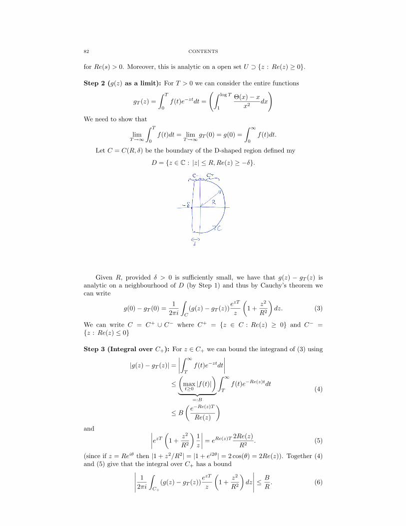
82 CONTENTS
for Re(s) > 0. Moreover, this is analytic on a open set U ⊃ z : Re(z) ≥ 0.
Step 2 (g(z) as a limit): For T > 0 we can consider the entire functions
gT (z) =∫ T
0
f(t)e−ztdt =
(∫ log T
1
Θ(x)− xx2
dx
)We need to show that
limT→∞
∫ T
0
f(t)dt = limT→∞
gT (0) = g(0) =∫ ∞
0
f(t)dt.
Let C = C(R, δ) be the boundary of the D-shaped region defined my
D = z ∈ C : |z| ≤ R,Re(z) ≥ −δ.
Given R, provided δ > 0 is sufficiently small, we have that g(z) − gT (z) isanalytic on a neighbourhood of D (by Step 1) and thus by Cauchy’s theorem wecan write
g(0)− gT (0) =1
2πi
∫C
(g(z)− gT (z))ezT
z
(1 +
z2
R2
)dz. (3)
We can write C = C+ ∪ C− where C+ = z ∈ C : Re(z) ≥ 0 and C− =z : Re(z) ≤ 0
Step 3 (Integral over C+): For z ∈ C+ we can bound the integrand of (3) using
|g(z)− gT (z)| =∣∣∣∣∫ ∞T
f(t)e−ztdt∣∣∣∣
≤(
maxt≥0|f(t)|
)︸ ︷︷ ︸
=:B
∫ ∞T
f(t)e−Re(z)tdt
≤ B(e−Re(z)T
Re(z)
)(4)
and ∣∣∣∣ezT (1 +z2
R2
)1z
∣∣∣∣ = eRe(z)T2Re(z)R2
. (5)
(since if z = Reiθ then |1 + z2/R2| = |1 + ei2θ| = 2 cos(θ) = 2Re(z)). Together (4)and (5) give that the integral over C+ has a bound∣∣∣∣∣ 1
2πi
∫C+
(g(z)− gT (z))ezT
z
(1 +
z2
R2
)dz
∣∣∣∣∣ ≤ B
R. (6)
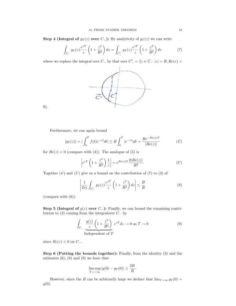
12. PRIME NUMBER THEOREM 83
Step 4 (Integral of gT (z) over C−): By analyticity of gT (z) we can write∫C−
gT (z)ezT
z
(1 +
z2
R2
)dz =
∫C′−
gT (z)ezT
z
(1 +
z2
R2
)dz (7)
where we replace the integral over C− by that over C ′− = z ∈ C : |z| = R,Re(z) <
0.
Furthermore, we can again bound
|gT (z)| = |∫ T
0
f(t)e−ztdt| ≤ B∫ T
0
|e−zt|dt =Be−Re(z)T
|Re(z)|(4′)
for Re(z) < 0 (compare with (4)). The analogue of (5) is∣∣∣∣ezT (1 +z2
R2
)1z
∣∣∣∣ = eRe(z)T2|Re(z)|R2
. (5′)
Together (4’) and (5’) give us a bound on the contribution of (7) to (3) of∣∣∣∣∣ 12πi
∫C′−
gT (z)ezT
z
(1 +
z2
R2
)dz
∣∣∣∣∣ ≤ B
R(8)
(compare with (6)).
Step 5 (Integral of g(z) over C−): Finally, we can bound the remaining contri-bution to (3) coming from the integralover C− by∫
C−
g(z)z
(1 +
z2
R2
)︸ ︷︷ ︸
Independent of T
ezT dz → 0 as T → 0 (9)
since Re(z) < 0 on C−.
Step 6 (Putting the bounds together): Finally, from the identity (3) and theestimates (6), (8) and (9) we have that
lim supT→+∞
|g(0)− gT (0)| ≤ 2BR.
However, since the R can be arbitrarily large we deduce that limT→∞ gT (0) =g(0).
84 CONTENTS
12.5. Proof of the Prime Number Theorem. It is actually easier to firstshow the following.
Lemma 12.10. Θ(x) ∼ x as x→ +∞
Proof. Assume that λ > 1 we can find xn → +∞ such that Θ(xn) ≥ λxn.Since Θ(x) is monotone increasing:∫ ∞
1
Θ(x)− xx2
dx ≥∞∑k=1
(λxk
∫ λxk
xk
1x2dx−
∫ λxk
xk
1xdx
)
=∞∑k=1
(∫ λ
1
1x2dx−
∫ λ
1
1xdx
)︸ ︷︷ ︸(By change of variables)
=∞∑k=1
((1− 1
λ
)− log λ
)︸ ︷︷ ︸
>0
= +∞.
This contradicts the integral converging.On the other hand, assume that λ < 1 we can find xn → +∞ such that
θ(xn) ≤ λxn we again show that the integral doesn’t converge.Either way, we see that Θ(x) ∼ x as x→ +∞.
This leads to the final result.
Theorem 12.11 (Prime Number Theorem).
π(x) ∼ x
log xas x→ +∞.
Proof. We can bound
Θ(x) =∑p≤x
log p
≤∑p≤x
log x = π(x) log x
For any ε > 0,
Θ(x) ≥∑
x1−ε≤p≤x
log p
≥ (1− ε) log x∑
x1−ε≤p≤x
1
≥ (1− ε) log x
π(x)− π(x1−ε)︸ ︷︷ ︸≤x1−ε
Since ε > 0 is arbitrary, together these show that π(x) ∼ x
log x .
Application 12.12 (More on the Riemann zeta function). Recall that we definethe Riemann zeta function by
ζ(s) =∞∑n=1
1ns
It is possible to show that this has an extension to C. We can write
Γ(s) =∫ ∞
0
xs−1e−xdx
13. FURTHER TOPICS 85
for σ = Re(s) and then
n−sΓ(s) =∫ ∞
0
xs−1e−nxdx.
Thus summing over n we have
ζ(s)Γ(s) =
( ∞∑n=1
1ns
)Γ(s) =
∫ ∞0
xs−1
ex − 1dx.
Lemma 12.13. For σ = Re(s) > 1,
ζ(s) = −Γ(1− s)2πi
∫C
(−z)s−1
ez − 1dz
where C runs from ∞ to 0, an infinitesimal circle about 0, followed by 0 to ∞.
Proof. We can write the integral as
−Γ(1− s)2πi
∫ ∞0
xs−1e−(s−1)πi
ee−(s−1)πi − 1dx+
Γ(1− s)2πi
∫ ∞0
xs−1e(s−1)πi
ee−(s−1)πi − 1dx
which is equal to 2i sin((s−1)πζ(s)Γ(s)) (using that Γ(s)Γ(1−s) = π/ sin(πs)).
In particular, the Right Hand Side of the formula is meromorphic for all s. Theintegral is entire in s. Moreover, Γ(1−s) is meromorphic with poles at s = 1, 2, · · · .(The poles at n ≥ 2 must actually cancel with the zeros of the integral since wealready know that ζ(s) is analytic there. However, the integral at s = 1 has value1.
Corollary 12.14. ζ(s)(s − 1) is an entire function (i.e., ζ(s) has a simplezero at s = 1).
13. Further Topics
There are a number of topics which would have fitted nicely into the coursewith more time.
13.1. Weierstrass’s elliptic function. If ω1, ω2 ∈ C such that Im(ω1/ω2)then we can consider the set of points
L = 2n1ω1 + 2n2ω2 : n1, n2 ∈ Z ⊂ C
Definition 13.1. We can define the Weierstrass elliptic functions are definedby
P (z) =1z2
+∑ω∈L
1z − w2
− 1w2
In particular, we have that P (z + 2ωi) = P (z) for i = 1, 2..
Theorem 13.2. This has a Laurent series expansion
P (z) =1z2
+120g2z
2 +128g3z
4 +O(z6).
where
g2(ω1, ω2) = 60∑
ω∈L−0
1w4
and g3(ω1, ω2) = 60∑
ω∈L−0
1w6
The coefficients satisfy g2(λω1, λω2) = λ−4g2(ω1, ω2) and g3(λω1, λω2) = λ−6g3(ω1, ω2),for λ > 0.
We can let τ = ω1/ω2 with Im(τ) > 0 be the period ratio and consider g2(τ) =g2(1, ω2/ω1) and g3(τ) = g3(1, ω2/ω1).
86 CONTENTS
Definition 13.3. The modular discriminant ∆ is defined as
∆(τ) = g32 − 27g2
3
This is studied in its own right, as a cusp form, in modular form theory (thatis, as a function of the period lattice).
Theorem 13.4. The discriminant is a modular form of weight 12. That is,under the action of the modular group, it transforms as
∆(zτ + b
cτ + d
)= (cτ + d)12∆(τ)
with a, b, c, d being integers, with ad− bc = 1.
13.2. Picard’s Little theorem. These describe the values of entire functions.
Theorem 13.5 (Picard’s Little Theorem). A non-constant entire function takesevery value , except at most one.
13.3. Runge’s theorem. This deals with approximations on compact sets.
Theorem 13.6 (Runge). Let U be a (simply-connected) domain. Then anyfunction analytic in U can be approximated uniformly on compact sets K ⊂ U bypolynomials, i.e., for each ε > 0 there is a polynomial p(z) with complex coefficientssuch that |f(z)− p(z)| < ε for all z ∈ K.
13.4. Conformality: Property of analytic maps. Any complex numberz = reiθ where r = |z| and θ = arg(z) is defined up to a multiple of 2π.
Let f : U → C be analytic and let γ be a smooth contour in U represented bta parameterization z : [a, b]→ C and let a < t0 < b be such that z′(t0) 6= 0.
Definition 13.7. Let U be an open neighbourhood. We say that f : U → Cis conformal on U if for each z0 ∈ U the function f is complex differentiable at z0
and f ′(z0) 6= 0 exists.
This has a more natural interpretation.
Lemma 13.8. f is conformal if and only if it preserves angles, i.e., given twosmooth paths γ1, γ2 : [0, 1]→ C with γ1(0) = γ2(0) we have that
arg (γ′1(0)− γ′2(0)) = arg ((f γ1)′(0)− (f γ2)′(0)) .
Proof. We can write γj(t) = xj(t) + iyj(t) and denote z0 = γ1(0) = γ2(0).Let f(z) = f(x+ iy) = u(x, y)+ iv(x, y). Suppose that γ′1(0) = γ′2(0). We can write(f γj)′(0) = f ′(γj(0).γj(0) for j = 1, 2. Thus
arg((f γj)′(0)) = arg(f ′(γj(0)) + arg(γj(0))
up to a multiple of 2π. We can then write
arg((f γ1)′(0))− arg((f γ2)′(0)) = arg(γ′1(0))− arg(γ′2(0))
up to a multiple of 2π.
Theorem 13.9. Analytic maps are conformal at all points at all points z0 suchthat f ′(z0) 6= 0
Method I: This can be illustrated by considering two two orthogonal familiesfamilies of contours such as the vertical lines and horizontal lines (or concentriccircles and radial lines). Let f(z) = u(x, y) + iv(x, y) with vertical lines x = α andhorizontal lines y = β.
Consider the the image of 2 perpendicular curves passing through z0, i.e., z0 =α + iβ. The image of the line x = α is now z = u(α, y) + iv(α, y) for y ∈ R. Theimage of the line y = β is now z = u(x, β) + iv(x, β). for x ∈ R.
14. PROBLEMS 87
Method II: Consider the so-called level curves of f(z) = u(z) + iv(z), i.e.,u(x, y) = α and v(x, y) = β. In particular, these curves are the ones mappedto the straight lines u = α and β = v.
Provided f ′(z0) 6= 0 we have that the angle between these preimages is θ = π/2.
Example 13.10 (Method I). Let f(z) = ez then f ′(z) = ez 6= 0 everywhere.Writing z = x+ iy gives f(z) = ex(cos θ + i sin θ).
If x = α then u = eα cos y and v = eα cos y with y ∈ R a parameter, i.e.,u2 + v2 = e2α which describes a circle.
If y = α then u+ iv = ex(cosβ + i sinβ). Thus uv = tan(β), i.e., a straight line
through the origin at angle β.
Example 13.11 (Method II). Let f(z) = z2 then f ′(z) = 2z =6= 0 except atz = 0. Writing f(z) = u + iv, the preimage of u = α are those x + iy such thatu(x, y) = α and the preimage of v = β are those x+ iy such that v(x, y) = β.
If x = α then u = eα cos y and v = eα cos y with y ∈ R a parameter, i.e.,u2 + v2 = e2α which describes a circle.
If y = α then u+ iv = ex(cosβ + i sinβ). Thus uv = tan(β), i.e., a straight line
through the origin at angle β.Thus z2 = (x+iy)2 = (x2−y2)+i2xy. The level sets correspond to x2−y2 = α
or 2xy = β.
Remark 13.12. In practise, it can be difficult to find the appropriate constantsfor these mappings. This involves numerical evaluation of elliptic integrals.
13.5. Functions of several complex variables. We can consider analyticfunctions f : U → C, where U ⊂ C2 is an open set. We can define analytic-ity in terms of the convergence of power series in two variables (on poly disksB(z0, w0, ε1, ε2) = (z, w) ∈ C2 : |z − z0| < ε1, |w − w0| < ε2) upon which we canapply the Cauchy theorem twice to write
f(z, w) = − 14π2
∫C(z0,ε1
∫C(z0,ε1
f(z, w)(z − z0)(w − w0)
dzdw
There are two particularly interesting theorems: The Bochner Tube Theorem andHartog’s Theorem
Theorem 13.13 (Bochner Tube theorem). Let Ω ⊂ R2 be a connected open setand let
co(Ω) = λx+ (1− λ)y : x, y ∈ Ω, 0 ≤ λ ≤ 1be the convex hull. If f : Ω + iR2 → C is analytic then f : co(Ω) + iR2 → C
Theorem 13.14 (Hartog Theorem). Assume that f : B(z0, w0, ε1/2, ε2/2)→ Cis analytic in two variables and f(·, w) : B(z0, r1) → C is analytic in one variablefor each w ∈ B(w0, r2). Then f : B(z0, w0, ε1/2, ε2/2)→ C is also analytic.
14. Problems
14.1. Problems 1. .
1. Show that the preimage of a circle or a straight line in C is a circle on theRiemann sphere under stereographic projection.
2. Show that the metric on C coming from the stereographic projection of the usualEuclidean metric is given as follows: If z := π((x1, x2, x3)) and w := π((x′1, x
′2, x′3))
then
d(z, w) = d ((x1, x2, x3), (x′1, x′2, x′3)) =
|z − w|√(1 + |z|2)(1 + |w|2)
88 CONTENTS
whenever (x1, x2, x3), (x′1, x′2, x′3) 6= (0, 0, 1) (i.e., z, w 6=∞) and
d(z,∞) := d((x1, x2, x3), (0, 0, 1)) =2√
1 + |z|2
whenever (x1, x2, x3) 6= (0, 0, 1) (i.e., z 6=∞)
3. Given a complex matrix M =(a bc d
)we can associate a Mobius map TM :
C→ C of the form TM (z) = az+bcz+d . Given two Mobius maps, relate MT1T2 to MT1
and MT2 .
4. Find the Mobius transformation that takes:(1) The points −i,−1, i to the points −i, 0, i, respectively;(2) The points −1 + i, 0, 1− i to the points −1,−i, i, respectively;(3) The points 0, 1 + i, 1− i to the points 1,−i, i, respectively.
5. What is the image of the unit disk D = z ∈ C : |z| < 1 under the followingMobius maps:
(1) T (z) = z+iz−i ;
(2) T (z) = iz−1i−z ;
(3) T (z) = (1+i)z+(i−1)iz+1 ;
(4) T (z) = 2z−1z−2 ;
(5) T (z) =√
2z−1+i√2z+1−i ;
(6) T (z) = (1+i)z−1−iz+1 .
6. The cross ratio of four points z0, z1, z2, z3 ∈ C is given by
(z0, z1, z2, z3) =(z0 − z2)(z1 − z3)(z0 − z3)(z1 − z2)
.
If λ = (z0, z1, z2, z3) show that different permutations of the four numbers givescross-ratios with the values
λ, 1− λ, 1− 1λ,
11− λ
,λ
1− λ.
Show that these are all possible values.
Apollation circle packing
1. Show that if E is a circle of radius k then:(1) if we reflect in E a circle C of radius r whose centres are separated by
d > r + k then the image f(C) is a circle with radius k2r/(d2 − r2).(2) if we reflect in E a straight line at a distance b > k from the centre of E
then the image f(C) is a circle of radius k2/2b.
2. If a Mobius map f(z) = az+bcz+d takes real numbers to real numbers (i.e., t ∈ R =⇒
f(t) ∈ R) then show that a, b, c, d are all real numbers.
Classification of Mobius maps
3. Show that any Mobius map other than the identity must fix at least one pointand at most two.
14. PROBLEMS 89
4. Since we are assuming ad − bc = 1 show that we can write (a − d)2 + 4bc =(a− d)2 + 4ad− 4 = 0
5. Let f : C→ C be a Mobius map. Show that(1) If f(∞) =∞ then f(z) = αz + β, for some α, β ∈ C.(2) If f(∞) =∞ and f(0) = 0 then f(z) = αz, for some α ∈ C.
6. We say that two linear fractional transformations f1, f2 are conjugate if f2 =g−1f1g for some linear fractional map g. We can associate to the Mobius mapf(z) = az+b
cz+d the value tr(f) := a + d. Show that the value tr(f) is preserved byconjugacy, i.e., if f1, f2 are conjugate then tr(f1) = tr(f2).
7. Let f : C → C be a Mobius transformation. The non-identity Mobius transfor-mations are commonly classified into three types:
(1) parabolic (conjugate to z 7→ z + β with a single fixed point ∞);(2) elliptic (conjugate to z 7→ αz with |α| = 1 with two points 0,∞); and(3) loxodromic (everything else).
Show that:(1) Elliptic Mobius transformations correspond to tr(f)2 ∈ [0, 4);(2) Parabolic Mobius transformations correspond to tr(f)2 = 4;(3) Hyperbolic Mobius transformations (i.e., conjugate to z 7→ λz with 0 <
λ < 1 or λ ∈ (1,∞)) correspond to tr(f)2 ∈ (4,∞).
14.2. Problems 2. .
Here <z and =z stand for real and imaginary parts of the complex number z,respectively.
0. Let f(z) : C→ C be a continuous function. Is it true that(1) <f(z) and =f(z)(2) |f(z)| and (f(z))
are continuous functions?
1. Show that if f : U → C is analytic and there exist a ∈ C and a convergentsequence zn → z with zn, z ∈ U such that f(zn) = a then f |U= a. What happensif z 6∈ U?
2. Show that the equivalence of parameterizations of curves is an equivalence rela-tion.
3. Show that∫−γ f(w)dw = −
∫γf(z)dz for any closed curve γ.
4. Show that if R = [a, b]× [c, d] is a rectangle then(1) We can evaluate
∫∂Rdz = 0;
(2) We can evaluate∫∂R
(z − z0)dz = 0.
5. Write the Cauchy-Riemann equations in polar coordinares.
6. Let f : D → C be a function well-defined in the unit disc, such that partialderivatives exist everywhere and Cauchy-Riemann equations hold true. Is it truethat f is complex differentiable everywhere in the unit disc? Hint: consider f(z) =exp(−z−4).
90 CONTENTS
8. Find all holomorphic functions that map the unit disc to the real line.
9. Find domains of complex differentiablity of the following functions(1) f1(z) = |z|;(2) f2(z) = zz;(3) f3(z) = z.
14.3. Problems 3. .
1. Define the Bernoulli numbers by the series zez−1 =
∑∞n=0
Bnn! z
n. Prove that
B0
n!0!+
B1
(n− 1)!1!+ · · ·+ Bn−1
1!(n− 1)!=
1 if n = 10 if n > 1.
2. Compute∫γzez
2dz where:
(1) γ = [i,−i+ 2]; and(2) γ = x+ ix2 : 0 ≤ x ≤ 1.
3. Compute∫γ
sin(z)dz where γ = x+ ix : 0 ≤ x ≤ 1.
4. Let f : D→ D be an analytic map which is injective (i.e., f(z1) = f(z2) impliesz1 = z2) of the form f(z) =
∑∞n=1 anz
n. Show that the image has area:
Area(f(D)) = π
∞∑n=1
n2|an|2.
5. Let f : D× D→ C be a continuous function such that(1) for w ∈ D the map D 3 z 7→ f(z, w) ∈ C is analytic; and(2) for z ∈ D the map D 3 zw 7→ f(z, w) ∈ C is analytic.
Show that we can write f(z, w) =∑∞n=0
∑∞m=0 anmz
nwm, which converges abso-lutely for z, w ∈ D.
6. Use Cauchy’s theorem to evaluate∫C(0,1)
(z − az − b
)2
dz
where b < 1 and C(0, 1) = z ∈ C : |z| = 1.
7. Let f : U → C be an analytic function. Let z0 ∈ U with f ′(z0) 6= 0. Let C be asufficiently small circle centred at z0 then show
2πif ′(z0)
=∫
dz
f(z)− f(z0)
8. If f is analytic in U and z0 ∈ U define
g(z) =
f(z)−f(z0)
z−z0 if z 6= z0
f ′(z0) if z = z0.
Show that this is analytic.
9. Use Rouche’s theorem to show that :(1) z7 − 4z3 + z − 1 = 0 has three zeros inside the unit circle;(2) z7 + 5z3 − z − 2 = 0 has three zeros inside the unit circle.

14. PROBLEMS 91
10. Use Rouche’s theorem to show that z87 + 36z57 + 71z4 + z3 − z + 1(1) has 4 zeros inside the unit circle.(2) has 87 zeros inside the circle z ∈ C : |z| = 2.
14.4. Problems 4. .
1. If |a| > e then show that ez = azn has n roots in the unit disk D = z ∈ C : |z| <1.
2. Consider the following polynomials:(1) How many zeros of z7 − 2z5 + 6z3 − z + 1 are in the unit disk D;(2) How many zeros of z4 − 6z + 3 are in the annulus z ∈ C : 1 < |z| < 2;(3) How many zeros of z4−4z3+6z2−4z+3 are in the set z ∈ C : |z−1| < 1.
3. Let h be analytic in the unit disk D and assume that
|h(z)− h(w)| < |z − w|for all z, w ∈ D. Show that the function f : D → C defined by f(z) = h(z) + z isone-to-one.
4. Let a > 0. Show that if f : C → C is analytic and satisfies |f(z)| < |z|a then fis a polynomial of degree at most [a].
5. Show that if f : C→ C is analytic and satisfies |f(z)| > 1 whenever |z| > 1 thenf is a polynomial.
6. Show that if f : C → C is analytic, non-constant and has no zeros then theremust exist a sequence of points |zn| → ∞ such that f(zn)→ 0.
7. Let f : D → C be analytic and continuous on the closed unit disk D = z ∈C : |z| ≤ 1. Moreover, assume that:
(1) |f(z)| ≤M whenever |z| = 1 and Im(z) ≥ 0; and(2) |f(z)| ≤ N whenever |z| = 1 and Im(z) < 0.
Then show that |f(0)| ≤√NM .
8. Show that if f : C→ C is analytic and Im(f(z)) 6= 0 whenever |z| 6= 1 then f isconstant.
9. Show that if f is a polynomial and z ∈ C then either fn(z)→∞ as n→ +∞ orfk(z) : k ≥ 0 is a bounded set.
14.5. Problems 5. 1. Consider the family of functions fn : D → C definedby fn(z) = zn, n ≥ 1. Show that for all z ∈ D = z ∈ C : |z| < 1 we have thatfn(z) → 0 as n → ∞ and that the convergence is uniform on compact sets, butthat it is not uniform on D.
2. Give an example of a family of analytic functions fn : D → C, n ≥ 1, for whichfn(z) has precisely one zero, but fn converges uniformly on D to the function f = 0(i.e., the function which is identically zero).
3. Give an example of a family of analytic functions fn : C → C, n ≥ 1 suchthat fn → ∞ uniformly on C (i.e., for all compact sets K ⊂ C and M > 0 wehave that infz∈K |fn(z)| ≥M for sufficiently large n) but for which the derivativesf ′n : C→ C, n ≥ 1, neither tend to ∞ nor form a normal family.
92 CONTENTS
4. Given two domains U1, U2 and two points z1 ∈ U1 and z2 ∈ U2 show that thereexists an analytic bijection f : U1 → U2 such that f(z1) = z2. [Hint: Use theRiemann Mapping Theorem].
5. Find the image of the unit disk D with respect to the map z 7→ z + 1z . Find the
image of the upper half plane H with respect to the map z 7→√z2 − 1
6. Find an analytic bijection between the following domains:(1) R× (0, π) and H = z ∈ C : Im(z) > 0;(2) H− [0, ir] and H;(3) D and C− (−∞,− 1
4 ];(4) (R× (0, 2))− ((i−∞, i− ε] ∪ [i+ ε, i+∞)) and H;(5) H and the equilateral triangle.
7. Let U ⊂ C be defined by
z ∈ C : 0 < Re(z) < 1, 0 < Im(z) < 1 −∞⋃n=1
[12n,
12n
+ i12
].
(1) Show that U is (path) connected;(2) Show that U is simply connected;(3) Show that 0 ∈ ∂U in the boundary cannot be reached by a continuous
path from any point in U ;(4) Show that any analytic bijection f : U → D cannot extend to a continuous
map from the boundary ∂U (of U) to the unit circle ∂D.
8. Let U ⊂ C be defined by
z ∈ C : Im(z) > 0 and |z| < 1 −⋃
p/q∈Q
[0,
1qeiπp/q
].
Show that every point in the boundary ∂U can be reached by a continuous pathfrom any point in U . However, show that any analytic bijection f : U → D cannotextend to a continuous map from the boundary ∂U of U to the unit circle ∂D.
9. Consider an analytic bijection f : U → D that satisfies that for z0 ∈ U ∩ R wehave that f(z0) = 0 and f ′(z0) > 0. Show that if U is symmetric about the realaxis then f(z) = f(z).
10. Show that there is no analytic bijection between D and C.
14.6. Problems 6. .
1. Let f : U → D be an analytic bijection. Fix z0 ∈ U . Show that if f(z0) = 0 andf ′(z0) > 0 then f is uniquely determined (i.e., uniqueness in the Riemann MappingTheorem).
2. Let x1 < x2 < · · · < xn be on the real line. Let 0 < α1, · · · , αn < 2. Let
F (z) =C
(z − x1)1−αn · · · (z − xn)1−αn.
Show that if xi−1 < t < xi then
Arg(F (t)) = Arg(C)− (αi + αi+1 + · · ·+ αn).
Deduce that the image of R with respect to the map f(z) =∫ zz0F (w)dw is a
piecewise linear curve. Is this a closed curve?
14. PROBLEMS 93
3. Let f : P→ D be continuous. Assume that f extends to a bijection f : ∂P→ ∂Don the boundary. Show that f : P→ D is surjective.
4. Let g : U → C be analytic. Let D ⊂ U be a closed region whose boundary curveγ = ∂D is simple. Assume that g : γ → g(γ) is one-to-one. Show that g : D → g(D)is one-to-one. (This is Darboux’s theorem). [Hint: Use the Argument Principle]
5. Do questions 2 – 4 give another proof that the Schwartz-Christoffel formula givesan analytic bijection f : H→ P for a polygon P?
6. Consider the semi-infinite strip
S = x+ iy : − a < x < a and y > 0for a > 0. Use the Schwarz-Christoffel theorem to find the analytic bijection f :H→ S which extends to f(±1) = ±a and f(∞) =∞.
7. Consider the triangle ∆ in C with vertices at −1, 0 and i. Use the Schwarz-Christoffel theorem to find the analytic bijection f : H → ∆ which extends tof(−1) = i, f(1) = −1 and f(∞) = 0.
8. Derive the version of the Schwarz-Christoffel theorem for an analytic bijectionf : D→ P from the unit disk to a polygon.
9. Describe the image of the unit disk D under the map f(z) =∫ z
0(1− ξn)−2/ndξ,
for n ≥ 3.
10. Describe the image of the unit disk D under the map f(z) =∫ z
0(1− ξ4)−1(1 +
ξ4)−1/2dξ.
14.7. Problems 8. .
1. Let f : U → C be analytic. Assume that f never vanishes. If there is a pointz0 ∈ U such that |f(z0)| ≤ |f(z)|, for all z ∈ U then f is a constant.
2. Suppose that both f(z) and g(z) are analytic on D with |f(z)| = |g(z)| for|z| = 1. Show that if neither f(z) nor g(z) vanishes in D then there exists λ ∈ Cwith |λ| = 1 such that f = λg.
3. Suppose that f(z) is analytic on D and for 0 ≤ r < 1 defineA(r) = max|z|=r Ref(z).Show that unless f is a constant, A(r) is a strictly increasing function of r.
4. Does there exist an analytic function f : D→ D with f( 12 ) = 3
4 and f ′( 12 ) = 3
4?
5. Let f(z) = (z + 1)2 on U = z = x + iy : 0 ≤ x ≤ 2 and 0 ≤ y ≤ 1. Wheredoes |f(z)| have its maximum and minimum values?
6. Show that the function w(x, y) = ex sin(y) is harmonic.
7. Let f : U → C be analytic and non-zero. Show that log |f(z)| is harmonic.
8. Show Harnack’s principle: Let u1 ≤ u2 ≤ · · · be harmonic functions on an openset U . Then either uj → ∞ uniformly on compacts sets or there is a harmonicfunction u on U such that uj → u uniformly on compact sets. [Hint: Use Harnack’sInequality].
9. Find the harmonic conjugate of u(x, y) = y3 − 3x2y.

94 CONTENTS
10. Describe suitable domains for the following harmonic functions, and find theirharmonic conjugates of the following functions:
(i) 2x(1− y);(ii) 2x− x3 + 3xy2;(iii) sinh(x) sin(y);(iv) y/(x2 + y2).
11. Show that if v1, v2 are both harmonic conjugates of u then v1−v2 is a constant.
![STOCHASTIC STABILITY OF POLLICOTT{RUELLE RESONANCESzworski/damped.pdf · STOCHASTIC STABILITY OF POLLICOTT{RUELLE RESONANCES ... {Liverani [BKL], ... stability of Pollicott{Ruelle](https://img.pdfslide.net/doc/110x75/5c658aac09d3f28c6e8cee03/stochastic-stability-of-pollicottruelle-resonances-zworskidampedpdf-stochastic.jpg)