Embed Size (px)
Citation preview

DRAFT 1
Lectures on Kinetic Theory andMagnetohydrodynamics of Plasmas
(Oxford MMathPhys/MSc in Mathematical and Theoretical Physics)
Alexander A. Schekochihin†The Rudolf Peierls Centre for Theoretical Physics, University of Oxford, Oxford OX1 3NP, UK
Merton College, Oxford OX1 4JD, UK
(compiled on 11 May 2019)
These are the notes for my lectures on Kinetic Theory of Plasmas and on Magnetohy-drodynamics, taught since 2014 as part of the MMathPhys programme at Oxford. PartI contains the lectures on plasma kinetics that formed part of the course on KineticTheory, taught jointly with Paul Dellar and James Binney. Part II is an introduction tomagnetohydrodynamics, which was part of the course on Advanced Fluid Dynamics,taught jointly with Paul Dellar. These notes have evolved from two earlier courses:“Advanced Plasma Theory,” taught as a graduate course at Imperial College in 2008,and “Magnetohydrodynamics and Turbulence,” taught as a Mathematics Part III courseat Cambridge in 2005-06. I will be grateful for any feedback from students, tutors orsympathisers.
CONTENTS
Part I. Kinetic Theory of Plasmas 61. Kinetic Description of a Plasma 6
1.1. Quasineutrality 61.2. Weak Interactions 61.3. Debye Shielding 61.4. Micro- and Macroscopic Fields 81.5. Maxwell’s Equations 91.6. Vlasov–Landau Equation 101.7. Collision Operator 101.8. Klimontovich’s Version of BBGKY 111.9. So What’s New and What Now? 13
2. Equilibrium and Fluctuations 142.1. Plasma Frequency 142.2. Slow vs. Fast 152.3. Multiscale Dynamics 162.4. Hierarchy of Approximations 17
2.4.1. Linear Theory 172.4.2. Quasilinear Theory (QLT) 182.4.3. Weak-Turbulence Theory 182.4.4. Strong-Turbulence Theory 19
3. Linear Theory: Plasma Waves, Landau Damping and Kinetic Instablities 193.1. Initial-Value Problem 193.2. Calculating the Dielectric Function: the “Landau Prescription” 23
† E-mail: [email protected]
2 A. A. Schekochihin
3.3. Solving the Dispersion Relation: Slow-Damping/Growth Limit 253.4. Langmuir Waves 263.5. Landau Damping and Kinetic Instabilities 273.6. Physical Picture of Landau Damping 293.7. Hot and Cold Beams 313.8. Ion-Acoustic Waves 333.9. Damping of Ion-Acoustic Waves and Ion-Acoustic Instability 353.10. Ion Langmuir Waves 363.11. Summary of Electrostatic (Longitudinal) Plasma Waves 363.12. Plasma Dispersion Function: Putting Linear Theory on Industrial Basis 37
3.12.1. Some Properties of Z(ζ) 383.12.2. Asymptotics of Z(ζ) 38
3.13. Alternatives to Landau’s Formalism 394. Energy, Entropy, Free Energy, Heating, Irreversibility and Phase Mixing 39
4.1. Energy Conservation and Heating 404.2. Entropy and Free Energy 424.3. Structure of Perturbed Distribution Function 444.4. Landau Damping Is Phase Mixing 464.5. Role of Collisions 474.6. Further Analysis of δf : the Case–van Kampen Mode 484.7. Free-Energy Conservation for a Landau-Damped Solution 50
5. General Kinetic Stability Theory 515.1. Linear Stability: Nyquist’s Method 51
5.1.1. Stability of Monotonically Decreasing Distributions 535.1.2. Penrose’s Instability Criterion 545.1.3. Bumps, Beams, Streams and Flows 565.1.4. Anisotropies 57
5.2. Nonlinear Stability: Thermodynamic Method 585.2.1. Gardner’s Theorem 605.2.2. Small Perturbations 615.2.3. Finite Perturbations 615.2.4. Anisotropic Equilibria 62
6. Nonlinear Theory: Two Pretty Nuggets 636.1. Nonlinear Landau Damping 636.2. Plasma Echo 63
7. Quasilinear Theory 637.1. General Scheme of QLT 637.2. Conservation Laws 65
7.2.1. Energy Conservation 667.2.2. Momentum Conservation 66
7.3. Quasilinear Equations for the Bump-on-Tail Instability in 1D 667.4. Resonant Region: QL Plateau and Spectrum 687.5. Energy of Resonant Particles 697.6. Heating of Non-Resonant Particles 707.7. Momentum Conservation 717.8. Validity of QLT 727.9. QLT in the Language of Quasiparticles 72
7.9.1. Plasmon Distribution 747.9.2. Electron Distribution 75

Oxford MMathPhys Lectures: Plasma Kinetics and MHD 3
8. Collisionless Relaxation 76
8.1. QLT and Beyond 76
8.2. QL Relaxation and Effective Collisionality 76
8.2.1. Lenard–Balescu Collision Integral 76
8.2.2. Kadomtsev–Pogutse Collision Integral 76
8.3. Quasinonlinear Theory a la Dupree 77
8.4. Stochastic Echo and Phase-Space Turbulence 779. Weak Turbulence 77
9.1. WT in the Language of Quasiparticles 77
9.2. General Scheme for Calculating Probabilities in WT 7710. Langmuir Turbulence 77
10.1. Electrons and Ions Must Talk to Each Other 77
10.2. Zakharov’s Equations 77
10.3. Derivation of Zakharov’s Equations 77
10.3.1. Scale Separations 77
10.3.2. Electron kinetics and ordering 77
10.3.3. Ponderomotive response 79
10.3.4. Electron fluid dynamics 80
10.3.5. Ion kinetics 81
10.3.6. Ion fluid dynamics 81
10.4. Secondary Instability of a Langmuir Wave 82
10.4.1. Decay Instability 82
10.4.2. Modulational Instability 82
10.5. Weak Langmuir Turbulence 82
10.6. Langmuir Collapse 82
10.7. Solitons and Cavitons 82
10.8. Kingsep–Rudakov–Sudan Turbulence 82
10.9. Pelletier’s Equilibrium Ensemble 82
10.10. Theories Galore 82Plasma Kinetics Problem Set 83Part II. Magnetohydrodynamics 9511. MHD Equations 95
11.1. Conservation of Mass 95
11.2. Conservation of Momentum 96
11.3. Electromagnetic Fields and Forces 97
11.4. Maxwell Stress and Magnetic Forces 98
11.5. Evolution of Magnetic Field 99
11.6. Magnetic Reynolds Number 99
11.7. Lundquist Theorem 100
11.8. Flux Freezing 101
11.9. Amplification of Magnetic Field by Fluid Flow 103
11.10. MHD Dynamo 104
11.11. Conservation of Energy 105
11.11.1. Kinetic Energy 106
11.11.2. Magnetic Energy 107
11.11.3. Thermal Energy 107
11.12. Virial Theorem 108
11.13. Lagrangian MHD 108

4 A. A. Schekochihin
12. MHD in a Straight Magnetic Field 10812.1. MHD Waves 108
12.1.1. Alfven Waves 11212.1.2. Magnetosonic Waves 11212.1.3. Parallel Propagation 11312.1.4. Perpendicular Propagation 11312.1.5. Anisotropic Perturbations: k‖ k⊥ 11412.1.6. High-β Limit: cs vA 115
12.2. Subsonic Ordering 11712.2.1. Ordering of Alfvenic Perturbations 11812.2.2. Ordering of Slow-Wave-Like Perturbations 11912.2.3. Ordering of Time Scales 11912.2.4. Summary of Subsonic Ordering 12012.2.5. Incompressible MHD Equations 12012.2.6. Elsasser MHD 12112.2.7. Cross-Helicity 12212.2.8. Stratified MHD 123
12.3. Reduced MHD 12512.3.1. Alfvenic Perturbations 12612.3.2. Compressive Perturbations 12712.3.3. Elsasser Fields and the Energetics of RMHD 12812.3.4. Entropy Mode 12912.3.5. Discussion 130
12.4. MHD Turbulence 13013. MHD Relaxation 130
13.1. Static MHD Equilibria 13113.1.1. MHD Equilibria in Cylindrical Geometry 13113.1.2. Force-Free Equilibria 133
13.2. Helicity 13413.2.1. Helicity Is Well Defined 13413.2.2. Helicity Is Conserved 13513.2.3. Helicity Is a Topological Invariant 136
13.3. J. B. Taylor Relaxation 13713.4. Relaxed Force-Free State of a Cylindrical Pinch 13813.5. Parker’s Problem and Topological MHD 139
14. MHD Stability and Instabilities 14014.1. Energy Principle 140
14.1.1. Properties of the Force Operator F [ξ] 14114.1.2. Proof of the Energy Principle (14.8) 142
14.2. Explicit Calculation of δW2 14314.2.1. Linearised MHD Equations 14314.2.2. Energy Perturbation 144
14.3. Interchange Instabilities 14514.3.1. Formal Derivation of the Schwarzschild Criterion 14514.3.2. Physical Picture 14614.3.3. Intuitive Rederivation of the Schwarzschild Criterion 146
14.4. Instabilities of a Pinch 14714.4.1. Sausage Instability 14914.4.2. Kink Instability 150

Oxford MMathPhys Lectures: Plasma Kinetics and MHD 5
15. Further Reading 15215.1. MHD Instabilities 15215.2. Resistive MHD 15215.3. Dynamo Theory and MHD Turbulence 15315.4. Hall MHD, Electron MHD, Braginskii MHD 15315.5. Double-Adiabatic MHD and Onwards to Kinetics 153
Magnetohydrodynamics Problem Set 155Appendix A. Kolmogorov Turbulence 162
A.1. Dimensional Theory of the Kolmogorov Cascade 162A.2. Exact Laws 162A.3. Intermittency 162A.4. Turbulent Mixing 162

6 A. A. Schekochihin
PART I
Kinetic Theory of Plasmas
1. Kinetic Description of a Plasma
We shall study a gas consisting of charged particles—ions and electrons. In general,there may be many different species of ions, with different masses and charges, and, ofcourse, only one type of electrons.
I shall index particle species by α (α = e for electrons, α = i for ions). Each ischaracterised by its mass mα and charge qα = Zαe, where e is the magnitude of theelectron charge and Zα is a positive or negative integer (e.g., Ze = −1).
1.1. Quasineutrality
We shall always assume that plasma is neutral overall:∑α
qαNα = eV∑α
Zαnα = 0, (1.1)
where Nα is the number of the particles of species α, nα = Nα/V is their mean numberdensity and V the volume of the plasma. This condition is known as quasineutrality.
1.2. Weak Interactions
Interaction between charged particles is governed by the Coulomb potential:
Φ(|r(α)i − r(α′)
j |)
= − qαqα′
|r(α)i − r(α′)
j |, (1.2)
where by r(α)i I mean the position of the i-th particle of species α. We can safely
anticipate that we will only be able to have a nice closed kinetic description if the gas isapproximately ideal, i.e., if particles interact weakly, viz.,
kBT Φ ∼ e2
∆r∼ e2n1/3, (1.3)
where kB is the Boltzmann constant, which will henceforth be absobed into the tem-perature T , and ∆r ∼ n−1/3 is the typical interparticle distance. Let us see what thiscondition means and implies physically.
1.3. Debye Shielding
Let us consider a plasma in thermodynamic equilibrium (as one does in statisticalmechanics, I will refuse to discuss, for the time being, how exactly it got there). Take oneparticular particle, of species α. It creates an electric field around itself, E = −∇ϕ; allother particles are sitting in this field (Fig. 1)—and, indeed, also affecting it, as we willsee below. In equilibrium, the densities of these particles ought to satisfy Boltzmann’sformula:
nα′(r) = nα′ e−qα′ϕ(r)/T ≈ nα′ −
nα′qα′ϕ
T, (1.4)
where nα′ is the mean density of particles of species α′ and ϕ(r) is the electrostaticpotential, which depends on the distance r from our “central” particle. As r →∞, ϕ→ 0and nα′ → nα′ . The exponential can be Taylor-expanded provided the weak-interactioncondition (1.3) is satisfied (eϕ T ).

Oxford MMathPhys Lectures: Plasma Kinetics and MHD 7
Figure 1. A particle amongst particles and its Debye sphere.
By the Gauss–Poisson law, we have
∇ ·E = −∇2ϕ = 4πqαδ(r) + 4π∑α′
qα′nα′
≈ 4πqαδ(r) + 4π∑α′
qα′ nα′︸ ︷︷ ︸= 0 by
quasineutral-ity
−
(∑α′
4πnα′q2α′
T
)︸ ︷︷ ︸
≡ 1/λ2D
ϕ. (1.5)
In the first line of this equation, the first term on the right-hand side is the chargedensity associated with the “central” particle and the second term the charge densityof the rest of the particles. In the second line, I used the Taylor-expanded Boltzmannexpression (1.4) for the particle densities and then the quasineutrality (1.1) to establishthe vanishing of the second term. The combination that has arisen in the last term asa prefactor of ϕ has dimensions of inverse square length, so we define the Debye lengthto be
λD ≡
(∑α
4πnαq2α
T
)−1/2
. (1.6)
Using also the obvious fact that the solution of (1.5) must be spherically symmetric, werecast this equation as follows
1
r2
∂
∂rr2 ∂ϕ
∂r− 1
λ2D
ϕ = −4πqαδ(r). (1.7)
The solution to this that asymptotes to the Coulomb potential ϕ → qα/r as r → 0 andto zero as r →∞ is
ϕ =qαre−r/λD . (1.8)
Thus, in a quasineutral plasma, charges are shielded on typical distances ∼ λD.Obviously, this calculation only makes sense if the “Debye sphere” has many particles
in it, viz., if
nλ3D 1. (1.9)
Let us check that this is the case: indeed,
nλ3D ∼ n
(T
ne2
)3/2
=
(T
n1/3e2
)3/2
1, (1.10)

8 A. A. Schekochihin
provided the weak-interaction condition (1.3) is satisfied. The quantity nλ3D is called the
plasma parameter.
1.4. Micro- and Macroscopic Fields
This calculation tells us something very important about electromagnetic fields in aplasma. Let E(micro)(r, t) and B(micro)(r, t) be the exact microscopic fields at a givenlocation r and time t. These fields are responsible for interactions between particles. Ondistances l λD, these will be essentially just two-particle interactions—binary collisionsbetween particles in a vacuum, just like in a neutral gas (except the interparticle potentialis a Coulomb potential). In contrast, on distances l & λD, individual particles’ fields areshielded and what remains are fields due to collective influence of large numbers ofparticles—macroscopic fields:
E(micro) = 〈E(micro)〉︸ ︷︷ ︸≡ E
+δE, B(micro) = 〈B(micro)〉︸ ︷︷ ︸≡ B
+δB, (1.11)
where the macroscopic fields E and B are averages over some intermediate scale l suchthat
∆r ∼ n−1/3 l λD. (1.12)
Such averaging is made possible by the condition (1.9).
Thus, plasma has a new feature compared to neutral gas: because the Coulombpotential is long-range (∝ 1/r), the fields decay on a length scale that is long comparedto the interparticle distances [λD ∆r ∼ n−1/3 according to (1.9)] and so, besidesinteractions between individual particles, there are also collective effects: interaction ofparticles with mean macroscopic fields due to all other particles.
Before I use this approach to construct a description of the plasma as a continuum (onscales & λD), let us check that particles travel sufficiently long distances between collisionsin order to feel the macroscopic fields, viz., that their mean free paths λmfp λD. Themean free path can be estimated in terms of the collision cross-section σ:
λmfp ∼1
nσ∼ T 2
ne4(1.13)
because σ ∼ d2 and the effective distance d by which the particles have to approacheach other in order to have significant Coulomb interaction is inferred by balancing theCoulomb potential energy with the particle temperature, e2/d ∼ T . Using (1.13) and(1.6), we find
λmfp
λD∼ T 2
ne4
(ne2
T
)1/2
∼ nλ3D 1, q.e.d. (1.14)
Thus, it makes sense to talk about a particle travelling long distances experiencing themacroscopic fields exerted by the rest of the plasma collectively before being deflectedby a much larger, but also much shorter-range, microscopic field of another individualparticle.

Oxford MMathPhys Lectures: Plasma Kinetics and MHD 9
1.5. Maxwell’s Equations
The exact microscopic fields satisfy Maxwell’s equations and, as Maxwell’s equationsare linear, so do the macroscopic fields: by direct averaging,
∇ · 〈E(micro)〉 = 4π〈σ(micro)〉, (1.15)
∇ · 〈B(micro)〉 = 0, (1.16)
∇× 〈E(micro)〉+1
c
∂〈B(micro)〉∂t
= 0, (1.17)
∇× 〈B(micro)〉 − 1
c
∂〈E(micro)〉∂t
=4π
c〈j(micro)〉. (1.18)
The new quantities here are the averages of the microscopic charge density σ(micro) andthe microscopic current density j(micro). How do we calculate them?
Clearly, they depend on where all the particles are at any given time and how fastthese particles move. We can assemble all this information in one function:
Fα(r,v, t) =
Nα∑i=1
δ3(r − r(α)
i (t))δ3(v − v(α)
i (t)), (1.19)
where r(α)i (t) and v
(α)i (t) are the exact phase-space coordinates of particle i of species
α at time t, i.e., these are the solutions of the exact equations of motion for all theseparticles moving in microscopic fields E(micro)(t, r) and B(micro)(t, r). The function Fαis called the Klimontovich distribution function. It is a random object (i.e., it fluctuateson scales λD) because it depends on the exact particle trajectories, which depend onthe exact microscopic fields. In terms of this distribution function,
σ(micro)(r, t) =∑α
qα
∫d3v Fα(r,v, t), (1.20)
j(micro)(r, t) =∑α
qα
∫d3v vFα(r,v, t). (1.21)
We now need to average these quantities for use in (1.15) and (1.18). We shall assumethat the average over microscales (1.12) and the ensemble average (i.e., average overmany different initial conditions) are the same. The ensemble average of Fα is an objectfamiliar from the kinetic theory of gases, the so-called one-particle distribution function:
〈Fα〉 = f1α(r,v, t) (1.22)
(I shall henceforth omit the subscript 1). If we learn how to compute fα, then we canaverage (1.20) and (1.21), substitute into (1.15) and (1.18), and have the following set ofmacroscopic Maxwell’s equations:
∇ ·E = 4π∑α
qα
∫d3v fα(r,v, t), (1.23)
∇ ·B = 0, (1.24)
∇×E +1
c
∂B
∂t= 0, (1.25)
∇×B − 1
c
∂E
∂t=
4π
c
∑α
qα
∫d3v vfα(r,v, t). (1.26)

10 A. A. Schekochihin
1.6. Vlasov–Landau Equation
We now need an evolution equation for fα(r,v, t), hopefully in terms of the macroscopicfields E(r, t) andB(r, t), so we can couple it to (1.23–1.26) and thus have a closed systemof equations describing our plasma.
The process of deriving it starts with Liouville’s theorem and is a direct generalisationof the BBGKY procedure familiar from gas kinetics (e.g., Dellar 2015)1 to the somewhatmore cumbersome case of a plasma:
—many species α;—Coulomb potential for interparticle collisions (with some attendant complications to
do with its long-range nature: in brief, use Rutherford’s cross section and cut off long-range interactions at λD; this is described in many textbooks and plasma-physics courses,e.g., Parra 2018a);
—presence of forces due to the macroscopic fields E and B.The result of this derivation is
∂fα∂t
+ fα, H1α =
(∂fα∂t
)c
. (1.27)
The Poisson bracket contains H1α, the Hamiltonian for a single particle of species αmoving in the macroscopic electromagnetic field—all the microscopic fields δE2 are goneinto the collision operator on the right-hand side, of which more will be said shortly (§1.7).
Technically speaking, we ought to be working with canonical variables, but dealingwith canonical momenta is an unnecessary complication and so I shall stick to the (r,v)representation of the phase space. Then (1.27) takes the form of Liouville’s equation, butwith microscopic fields hidden inside the collision operator:
∂fα∂t
+∂
∂r·(rfα
)+
∂
∂v·(vfα
)=
(∂fα∂t
)c
, (1.28)
where
r = v, v =qαmα
(E +
v ×Bc
). (1.29)
This gives us the Vlasov–Landau equation:
∂fα∂t
+ v ·∇fα +qαmα
(E +
v ×Bc
)· ∂fα∂v
=
(∂fα∂t
)c
. (1.30)
Any other macroscopic force that the plasma might be subject to (e.g., gravity) canbe added to the Lorentz force in the third term on the left-hand side, as long as itsdivergence in velocity space is (∂/∂v) · force = 0. Equation (1.30) is closed by Maxwell’sequations (1.23–1.26).
1.7. Collision Operator
Finally, a few words about the plasma collision operator, originally due to Landau(1936) (the same considerations apply to the the more general Lenard–Balescu operator;see Balescu 1963 and §8.2.1). It describes two-particle collisions both within the species αand with other species α′ and so depends both on fα and on all other fα′ . Its derivation isleft to you as an exercise in BBGKY’ing, calculating cross sections and velocity integrals(or in googling; shortcut: see Parra 2018a). In these Lectures, I shall largely focus on
1In §1.8, I will sketch Klimontovich’s version of this procedure (Klimontovich 1967).2δB turns out to be irrelevant as long as the particle motion is non-relativistic, v/c 1.

Oxford MMathPhys Lectures: Plasma Kinetics and MHD 11
collisionless aspects of plasma kinetics. Whenever we find ourselves in need of invokingthe collision operator, the important things about it for us will be its properties:• conservation of particles, ∫
d3v
(∂fα∂t
)c
= 0 (1.31)
(within each species α);• conservation of momentum,∑
α
∫d3vmαv
(∂fα∂t
)c
= 0 (1.32)
(same-species collisions conserve momentum, whereas different-species collisions conserveit only after summation over species—there is friction of one species against another; forexample, the friction of electrons against the ions is the Ohmic resistivity of the plasma);• conservation of energy, ∑
α
∫d3v
mαv2
2
(∂fα∂t
)c
= 0; (1.33)
• Boltzmann’s H-theorem: the kinetic entropy
S = −∑α
∫d3r
∫d3v fα ln fα (1.34)
cannot decrease, and, as S is conserved by all the collisionless terms in (1.30), the collisionoperator must have the property that
dS
dt= −
∑α
∫d3r
∫d3v
(∂fα∂t
)c
ln fα > 0, (1.35)
with equality obtained if and only if fα is a local Maxwellian;• unlike the Boltzmann operator for neutral gases, the Landau operator expresses
the cumulative effect of many glancing (rather than “head-on”) collisions (due to thelong-range nature of the Coulomb interaction) and so it is a Fokker–Planck operator:3(
∂fα∂t
)c
=∑α′
∂
∂vi
(A
(αα′)i [fα′ ] +
∂
∂vjD
(αα′)ij [fα′ ]
)fα, (1.36)
where the drag A(αα′)i [fα′ ] and diffusion D
(αα′)ij [fα′ ] coefficients are integral (in v space)
functionals of fα′ . The Fokker–Planck form (1.36) of the Landau operator means that itdescribes diffusion in velocity space and so will erase sharp gradients in fα with respectto v—a property that we will find very important in §4.
1.8. Klimontovich’s Version of BBGKY
By way of a technical digression, let me outline the (beginning of the) derivation of (1.30) dueto Klimontovich (1967). Consider the Klimontovich distribution function (1.19) and calculate
3The simplest example that I can think of in which the collision operator is a velocity-spacediffusion opeartor of this kind is the gas of Brownian particles [each with velocity described byLangevin’s equation (10.61)]. This is treated in detail in §6.9 of Schekochihin (2018).

12 A. A. Schekochihin
its time derivative: by the chain rule,
∂Fα∂t
=−∑i
dr(α)i (t)
dt·[∂
∂rδ3(r − r(α)i (t)
)δ3(v − v(α)
i (t))]
−∑i
dv(α)i (t)
dt·[∂
∂vδ3(r − r(α)i (t)
)δ3(v − v(α)
i (t))]. (1.37)
First, because r(α)i (t) and v
(α)i (t) obviously do not depend on the phase-space variables r and
v, the derivatives ∂/∂r and ∂/∂v can be pulled outside, so the right-hand side of (1.37) can bewritten as a divergence in phase space. Secondly, the particle equations of motion give us
dr(α)i (t)
dt= v
(α)i (t), (1.38)
dv(α)i (t)
dt=
qαmα
[E(micro)(r(α)i (t), t
)+v(α)i (t)×B(micro)
(r(α)i (t), t
)c
], (1.39)
which we substitute into the right-hand side of (1.37)—after it is written in the divergence form.
As the time derivatives of r(α)i (t) and v
(α)i (t) inside the divergence multiply delta functions
identifying r(α)i (t) with r and v
(α)i (t) with v, we may replace r
(α)i (t) by r and v
(α)i (t) by v in
the right-hand sides of (1.38) and (1.39) when they go into (1.37). This gives (wrapping all thesums of delta functions back into Fα)
∂Fα∂t
= −∇ · (vFα)− ∂
∂v·[qαmα
(E(micro)(r, t) +
v ×B(micro)(r, t)
c
)Fα
]. (1.40)
Finally, because r and v are independent variables and the Lorentz force has zero divergence inv space, we find that Fα satisfies exactly
∂Fα∂t
+ v ·∇Fα +qαmα
(E(micro) +
v ×B(micro)
c
)· ∂Fα∂v
= 0 . (1.41)
This is the Klimontovich equation. There is no collision integral here because microscopic fieldsare explicitly present. The equation is closed by the microscopic Maxwell’s equations:
∇ ·E(micro) = 4π∑α
qα
∫d3v Fα(r,v, t), (1.42)
∇ ·B(micro) = 0, (1.43)
∇×E(micro) +1
c
∂B(micro)
∂t= 0, (1.44)
∇×B(micro) − 1
c
∂E(micro)
∂t=
4π
c
∑α
qα
∫d3v vFα(r,v, t). (1.45)
Now we separate the microscopic fields into mean (macroscopic) and fluctuating parts ac-cording to (1.11); also
Fα = 〈Fα〉︸︷︷︸≡ fα
+ δFα. (1.46)
Maxwell’s equations are linear, so averaging them gives the same equations for E and B interms of fα [see (1.23–1.26)] and for δE and δB in terms of δFα. Averaging the Klimontovichequation (1.41) gives the Vlasov–Landau equation:
∂fα∂t
+ v ·∇fα +qαmα
(E +
v ×Bc
)· ∂fα∂v
= − qαmα
⟨(δE +
v × δBc
)· ∂δFα∂v
⟩≡(∂fα∂t
)c
. (1.47)

Oxford MMathPhys Lectures: Plasma Kinetics and MHD 13
The macroscopic fields in the left-hand side satisfy the macroscopic Maxwell’s equations (1.23–1.26). The microscopic fluctuating fields δE and δB inside the average in the right-hand sidesatisfy microscopic Maxwell’s equations with fluctuating charge and current densities expressedin terms of δFα. Thus, the right-hand side is quadratic in δFα. In order to close this equation, weneed an expression for the correlation function 〈δFαδFα′〉 in terms of fα and fα′ . This is basicallywhat the BBGKY procedure plus truncation of velocity integrals based on an expansion in 1/nλ3
D
achieve. The result is the Landau collision operator (or the more precise Lenard–Balescu one;see Balescu 1963 and §8.2.1).
Further details are complicated (see Klimontovich 1967), but my aim here was just to showhow the fields are split into macroscopic and microscopic ones, with the former appearingexplicitly in the kinetic equation and the latter wrapped up inside the collision operator. Thepresence of the macroscopic fields and the consequent necessity for coupling the kinetic equationwith Maxwell’s equations for these fields is the main mathematical difference between the kineticsof neutral gases and the kinetics of plasmas.
1.9. So What’s New and What Now?
Let me summarise the new features that have appeared in the kinetic description of aplasma compared to that of a neutral gas.
• First, particles are charged, so they interact via Coulomb potential. The collisionoperator is, therefore, different: the cross-section is the Rutherford cross-section, mostcollisions are glancing (with interaction on distances up to the Debye length), leading todiffusion of the particle distribution function in velocity space. Mathematically, this ismanifested in the collision operator in (1.30) having the Fokker–Planck structure (1.36).
One can spin out of the Vlasov–Landau equation (1.30) a theory that is analogousto what is done with Boltzmann’s equation in gas kinetics (Dellar 2015): derivefluid equations, calculate viscosity, thermal conductivity, Ohmic resistivity, etc., of acollisionally dominated plasma, i.e., of a plasma in which the collision frequency of theparticles is much greater than all other relevant time scales. This is done in the sameway as in gas kinetics, but now applying the Chapman–Enskog procedure to the Landaucollision operator. This is quite a lot of work—and constitutes core textbook plasma-physics material (see Parra 2018a). In magnetised plasmas especially, the resulting fluiddynamics of the plasma are quite interesting and quite different from neutral fluids—weshall see some of this in Part II of these Lectures, while the classic treatment of thetransport theory can be found in Braginskii (1965); a great textbook on this is Helander& Sigmar (2005).4
• Secondly, Coulomb potential is long-range, so the electric and magnetic fields have amacroscopic (mean) part on scales longer than the Debye length—a particle experiencingthese fields is not undergoing a collision in the sense of bouncing off another particle,but is, rather, interacting, via the fields, with the collective of all the other particles.Mathematically, this manifests itself as a Lorentz-force term appearing in the right-handside of the Vlasov–Landau kinetic equation (1.30). The macroscopic E and B fields thatfigure in it are determined by the particles via their mean charge and current densitiesthat enter the macroscopic Maxwell’s equations (1.23–1.26).
In the case of neutral gas, all the interesting kinetic physics is in the collision operator,hence the focus on transport theory in gas-kinetic literature (see, e.g., the classic mono-graph by Chapman & Cowling 1991 if you want an overdose of this). In the collisionless
4See Krommes (2018) for a modernist approach.

14 A. A. Schekochihin
limit, the kinetic equation for a neutral gas,
∂f
∂t+ v ·∇f = 0, (1.48)
simply describes particles with some initial distribution ballistically flying in straightlines along their initial directions of travel. In contrast, for a plasma, even the collisionlesskinetics (and, indeed, especially the collisionless—or weakly collisional—kinetics) areinteresting and nontrivial because, as the initial distribution starts to evolve, it givesrise to charge densities and currents, which modify E and B, which modify fα, etc. Thisopens up a whole new conceptual world and it is on these effects involving interactionsbetween particles and fields that I shall focus here, in pursuit of maximum novelty.5
I shall also be in pursuit of maximum simplicity (well, “as simple as possible, but notsimpler”!) and so will mostly restrict my considerations to the “electrostatic approxima-tion”:
B = 0, E = −∇ϕ. (1.49)
This, of course, eliminates a huge number of interesting and important phenomenawithout which plasma physics would not be the voluminous subject that it is, but wecannot do them justice in just a few lectures (so see Parra 2018b for a course mostlydevoted to collisionless magnetised plasmas).
Thus, we shall henceforth focus on a simplified kinetic system, called the Vlasov–Poisson system:
∂fα∂t
+ v ·∇fα −qαmα
(∇ϕ) · ∂fα∂v
= 0, (1.50)
−∇2ϕ = 4π∑α
qα
∫d3v fα. (1.51)
Formally, considering a collisionless plasma6 would appear to be legitimate as long asthe collision frequency is small compared to the characteristic frequencies of any otherevolution that might be going on. What are the characteristic time scales (and lengthscales) in a plasma and what phenomena occur on these scales? These questions bringus to our next theme.
2. Equilibrium and Fluctuations
2.1. Plasma Frequency
Consider a plasma in equilibrium, in a happy quasineutral state. Suppose a populationof electrons strays from this equilibrium and upsets quasineutrality a bit (Fig. 2). If they
5Similarly interesting things happen when the field tying the particles together is gravity—aneven more complicated situation because, while the potential is long-range, rather like theCoulomb potential, gravity is not shielded and so all particles feel each other at all distances.This gives rise to remarkably interesting theory (Binney 2016).6Or, I stress again, a weakly collisional plasma. The collision operator is dropped in (1.50), butlet us not forget about it entirely even if the collision frequency is small; it will make a comeback in §4.

Oxford MMathPhys Lectures: Plasma Kinetics and MHD 15
Figure 2. A displaced population of electrons will set up a quasineutrality-restoring electricfield, leading to plasma oscillations.
have shifted by distance δx, the restoring force on each electron will be
meδx = −eE = −4πe2neδx ⇒ δx = − 4πe2neme︸ ︷︷ ︸≡ ω2
pe
δx, (2.1)
so there will be oscillations at what is known as the (electron) plasma frequency :
ωpe =
√4πe2neme
. (2.2)
Thus, we expect fluctuations of electric field in a plasma with characteristic frequenciesω ∼ ωpe (these are Langmuir waves; I will derive their dispersion relation rigorously in§3.4). These fluctuations are due to collective motions of the particles—so they are stillmacroscopic fields in the nomenclature of §1.4.
The time scale associated with ωpe is the scale of restoration of quasineutrality. Thedistance an electron can travel over this time scale before the restoring force kicks in,i.e., the distance over which quasineutrality can be violated, is (using the thermal speedvthe ∼
√T/me to estimate the electron’s velocity)
vthe
ωpe∼√
T
me
√me
e2ne=
√T
e2ne∼ λD, (2.3)
the Debye length (1.6)—not surprising, as this is, indeed, the scale on which microscopicfields are shielded and plasma is quasineutral (§1.3).
Finally, let us check that the plasma oscillations happen on collisionless time scales.The collision frequency of the electrons is
νe ∼vthe
λmfp=vthe
ωpe
ωpe
λmfp∼ λD
λmfpωpe ωpe, q.e.d., (2.4)
using (2.3) and (1.14).
2.2. Slow vs. Fast
The plasma frequency ωpe is only one of the characteristic frequencies (the largest)of the fluctuations that can occur in plasmas. We will think of the scales of all thesefluctuations as short and of the associated variation in time and space as fast. They occur

16 A. A. Schekochihin
against the background of some equilibrium state,7 which is either constant or variesslowly in time and space. The slow evolution and spatial variation of the equilibriumstate can be due to slowly changing, large-scale external conditions that gave rise to thisstate or, as we will discover soon, it can be due to the average effect of a sea of smallfluctuations.
Formally, what we are embarking on is an attempt to set up a mean-field theory,separating slow (large-scale) and fast (small-scale) parts of the distribution function:
f(r,v, t) = f0(εar,v, εt) + δf(r,v, t), (2.5)
where ε is some small parameter characterising the scale separation between fast andslow variation (note that this separation need not be the same for spatial and timescales, hence εa). To avoid clutter, I shall drop the species index where this does not leadto ambiguity.
For simplicity, I will drop the spatial dependence of the equilibrium distributionaltogether and consider homogeneous systems:
f0 = f0(v, εt), (2.6)
which also means E0 = 0 (there is no equilibrium electric field). Equivalently, we restrictall our considerations to scales much smaller than the characteristic system size. Formally,this equilibrium distribution can be defined as the average of the exact distribution overthe volume of space that we are considering and over time scales intermediate betweenthe fast and the slow ones:8
f0(v, t) = 〈f(r,v, t)〉 ≡ 1
∆t
∫ t+∆t/2
t−∆t/2dt′∫
d3r
Vf(r,v, t′), (2.7)
where ω−1 ∆t teq, where teq is the equilibrium time scale.
2.3. Multiscale Dynamics
We will find it convenient to work in Fourier space:
ϕ(r, t) =∑k
eik·rϕk(t), f(r,v, t) = f0(v, t) +∑k
eik·rδfk(v, t). (2.8)
Then the Poisson equation (1.51) becomes
ϕk =4π
k2
∑α
qα
∫d3v δfkα (2.9)
and the Vlasov equation (1.50) written for k = 0 (i.e., the spatial average of theequation) is
∂f0
∂t+∂δfk=0
∂t= − q
m
∑k
ϕ−kik ·∂δfk∂v
, (2.10)
7Or even just an initial state that is slow to change.8I use anglular brackets to denote this average, but it should be clear that this is not the samething as the average (1.11) that allowed us to separate macroscopic fields from microscopic ones.The latter was over sub-Debye scales, whereas our new average is over scales that are largerthan fluctuation scales but smaller than the system scales; both fluctuations and equilibriumare “macroscopic” in the language of §1.4.

Oxford MMathPhys Lectures: Plasma Kinetics and MHD 17
where we can replace ϕ−k = ϕ∗k because ϕ(r, t) must be real. Averaging over timeaccording to (2.7) eliminates fast variation and gives us
∂f0
∂t= − q
m
∑k
⟨ϕ∗kik ·
∂δfk∂v
⟩. (2.11)
The right-hand side of (2.11) gives us the slow evolution of the equilibrium (mean)distribution due to the effect of fluctuations (§§7, 8). In practice, the main question isoften how the equilibrium evolves and so we need a closed equation for the evolution of f0.This should be obtainable at least in principle because the fluctuating fields appearingin the right-hand side of (2.11) themselves depend on f0: indeed, writing the Vlasovequation (1.50) for the k 6= 0 modes, we find the following evolution equation for thefluctuations:
∂δfk∂t
+ ik · v δfk︸ ︷︷ ︸particle
streaming(phasemixing)
=q
mϕkik ·
∂f0
∂v︸ ︷︷ ︸wave-particleinteraction
(linear)
+q
m
∑k′
ϕk′ik′ · ∂δfk−k
′
∂v︸ ︷︷ ︸nonlinear
interactions
. (2.12)
The three terms that control the evolution of the perturbed distribution function in (2.12)represent the three physical effects that I shall focus on in these Lectures. The secondterm on the left-hand side represents free ballistic motion of particles (“streaming”). Itwill give rise to the phenomenon of phase mixing (§4) and, in its interplay with plasmawaves, to Landau damping and kinetic instabilities (§§3, 5.1). The first term on the right-hand side contains the interaction of the electric-field perturbations (waves) with theequilibrium particle distribution (§§3, 7). The second term on the right-hand side of (2.12)has nonlinear interactions between fluctuating fields and the perturbed distribution—itis negligible when fluctuation amplitudes are small enough (which, sadly, they rarelyare) and responsible for plasma turbulence (§§8–10) and other nonlinear phenomena (§6)when they are not.
The programme for determining the slow evolution of the equilibrium is “simple”:solve (2.12) together with (2.9), calculate the correlation function of the fluctuations,〈ϕ∗kδfk〉, as a functional of f0, and use it to close (2.11); then proceed to solve the latter.Obviously, this is impossible to do in most cases. But it is possible to construct a hierarchyof approximations to the answer and learn much interesting physics in the process.
2.4. Hierarchy of Approximations
2.4.1. Linear Theory
Consider first infinitesimal perturbations of the equilibrium. All nonlinear terms canthen be ignored, (2.11) turns into f0 = const and (2.12) becomes
∂δfk∂t
+ ik · v δfk =q
mϕkik ·
∂f0
∂v, (2.13)
the linearised kinetic equation. Solving this together with (2.9) allows one to find oscillat-ing and/or growing/decaying9 perturbations of a particular equilibrium f0. The theory
9We shall see (§4) that growing/decaying linear solutions imply the equilibrium distributiongiving/receiving energy to/from the fluctuations.

18 A. A. Schekochihin
for doing this is very well developed and contains some of the core ideas that give plasmaphysics its intellectual shape (§§3, 5.1).
Physically, the linear solutions will describe what happens over short term, viz., ontimes t such that
ω−1 t teq or tnl, (2.14)
where ω is the characteristic frequency of the perturbations, teq is the time after which theequilibrium starts getting modified by the perturbations [which depends on the amplitudeto which they can grow: see the right-hand side of (2.11); if perturbations do grow, i.e.,the equilibrium is unstable, they can modify the equilibrium by this mechanism so asto render it stable], and tnl is the time at which perturbation amplitudes become largeenough for nonlinear interactions between individual modes to matter [second term onthe right-hand side of (2.12); if perturbations grow, they can saturate by this mechanism].
2.4.2. Quasilinear Theory (QLT)
Suppose
teq tnl, (2.15)
i.e., growing perturbations start modifying the equilibrium before they saturate nonlinearly.Then the strategy is to solve (2.13) [together with (2.9)] for the perturbations, use theresult to calculate their correlation function needed in the right-hand side of (2.11), thenwork out how the equilibrium therefore evolves and hence how large the perturbationsmust grow in order for this evolution to turn the equilibrium from one causing theinstability to a stable one. This is a classic piece of theory, important conceptually—Iwill describe it in detail and do one example in §7 and another in Q9. In reality, however,it happens relatively rarely that unstable perturbations saturate at amplitudes smallenough for the nonlinear interactions not to matter (i.e., for tnl teq).
2.4.3. Weak-Turbulence Theory
Sometimes, one is not lucky enough to get away with QLT (so tnl . teq), but is luckyenough to have perturbations saturating nonlinearly at a small amplitude such that10
tnl ω−1, (2.16)
i.e., perturbations oscillate faster than they interact (this can happen for example becausepropagating wave packets do not stay together long enough to break up completely inone encounter). In this case, one can do perturbation theory treating the nonlinear termin (2.12) as small and expanding in the small parameter (ωtnl)
−1.Because waves are fast compared to nonlinear evolution in this approximation, it is
possible to “quantise” them (as indeed it is already possible to do in QLT), i.e., to treata nonlinear turbulent state of the plasma as a cocktail consisting of both “true” particles(ions and electrons) and “quasiparticles” representing electromagnetic excitations (§§7.9and 9.1).
Note that because the nonlinear term couples perturbations at different k’s (scales),this theory will lead to broad (power-law) fluctuation spectra.
We will not have sufficient time for this: it is a pity as the weak (or “wave”) turbulencetheory is quite an analytical tour de force—but it is a lot of work to do it properly! I willprovide an introduction to WT in §9. Classic texts on this are Kadomtsev (1965) (earlybut lucid) and Zakharov et al. (1992) (mathematically definitive); a recent textbook
10Note that the nonlinear time scale is typically inversely proportional to the amplitude;see (2.12).

Oxford MMathPhys Lectures: Plasma Kinetics and MHD 19
in Zakharov’s tradition is Nazarenko (2011), while the quasiparticle approach (withFeynman diagrams and all that) can be learned from Tsytovich (1995) or Kingsep (2004).Specifically on weak turbulence of Langmuir waves, there is a long, mushy review byMusher et al. (1995).
2.4.4. Strong-Turbulence Theory
If perturbations manage to grow to a level at which
tnl ∼ ω−1, (2.17)
we are a facing strong turbulence. This is actually what mostly happens. Theory of suchregimes tends to be of phenomenological/scaling kind, often in the spirit of the classicKolmogorov (1941) theory of hydrodynamic turbulence.11 Here are two examples, notnecessarily the best or most relevant, just mine: Schekochihin et al. (2009, 2016). No onereally knows how to do much beyond this sort of approach—and not for lack of trying(a recent but historically aware review is Krommes 2015). I will, nevertheless, try againin §§8 and 10.
3. Linear Theory: Plasma Waves, Landau Damping and KineticInstablities
Enough idle chatter, let us calculate! In this section, we are concerned with thelinearised Vlasov–Poisson system, (2.13) and (2.9):
∂δfkα∂t
+ ik · v δfkα =qαmα
ϕkik ·∂f0α
∂v, (3.1)
ϕk =4π
k2
∑α
qα
∫d3v δfkα. (3.2)
For compactness of notation, I will drop both the species index α and the wave numberk in the subscripts, unless they are necessary for understanding.
We will discover that electrostatic perturbations in a plasma described by (3.1) and(3.2) oscillate, can pass their energy to particles (damp) or even grow, sucking energyfrom the particles. We will also discover that it is useful to know some complex analysis.
3.1. Initial-Value Problem
We shall follow Landau’s original paper (Landau 1946) in considering an initial-valueproblem—because, as we will see, perturbations can be damped or grow, so it is notappropriate to think of them over t ∈ [−∞,+∞] (and—NB!!!—the damped perturbationsare not pure eignenmodes; see §4.3). So we look for δf(v, t) satisfying (3.1) with the initialcondition
δf(v, t = 0) = g(v). (3.3)
11A kind of exception is a very special case of strong Langmuir turbulence, which was extremelypopular in the 1970s and 80s. The founding documents on this are Zakharov (1972) and Kingsepet al. (1973), but there is a huge and sophisticated literature that followed. There is, alas, noparticularly good review, but see Thornhill & ter Haar (1978), Rudakov & Tsytovich (1978),Goldman (1984), Zakharov et al. (1985) and Robinson (1997) (I find the first of these the mostreadable of the lot). I will give an introduction to this topic in §10. Another, distinct, intellectualstrand is the “quasinonlinear” approach usually associated with the name of Dupree (1972), butreally due to Kadomtsev & Pogutse (1970, 1971), of which I will attempt to make some sensein §8 (based on Adkins 2018).

20 A. A. Schekochihin
(a) (b)
Figure 3. Lev Landau (1908-1968), great Soviet physicist, quintessential theoretician, authorof the Book, cult figure. It is a minor feature of his scientific biography that he wrote the twomost important plasma-physics papers of all time (Landau 1936, 1946). He also got a NobelPrize (1962), but not for plasma physics. (a) Cartoon by A. A. Yuzefovich (from Landau &Lifshitz 1976); the caption says “[And] Dau spake. . . ” (. . . unto the students, also depicted).(b) Landau’s mugshot from NKVD prison (1938), where he ended up for seditious talk and fromwhence he was released in 1939 after Kapitsa’s personal appeal to Stalin.
It is, therefore, appropriate to use Laplace transform to solve (3.1):
δf(p) =
∫ ∞0
dt e−ptδf(t) . (3.4)
It is a mathematical certainty that if there exists a real number σ > 0 such that
|δf(t)| < eσt as t→∞, (3.5)
then the integral (3.4) exists (i.e., is finite) for all values of p such that Re p > σ. Theinverse Laplace transform, giving us back our distribution function as a function of time,is then
δf(t) =1
2πi
∫ i∞+σ
−i∞+σ
dp eptδf(p), (3.6)
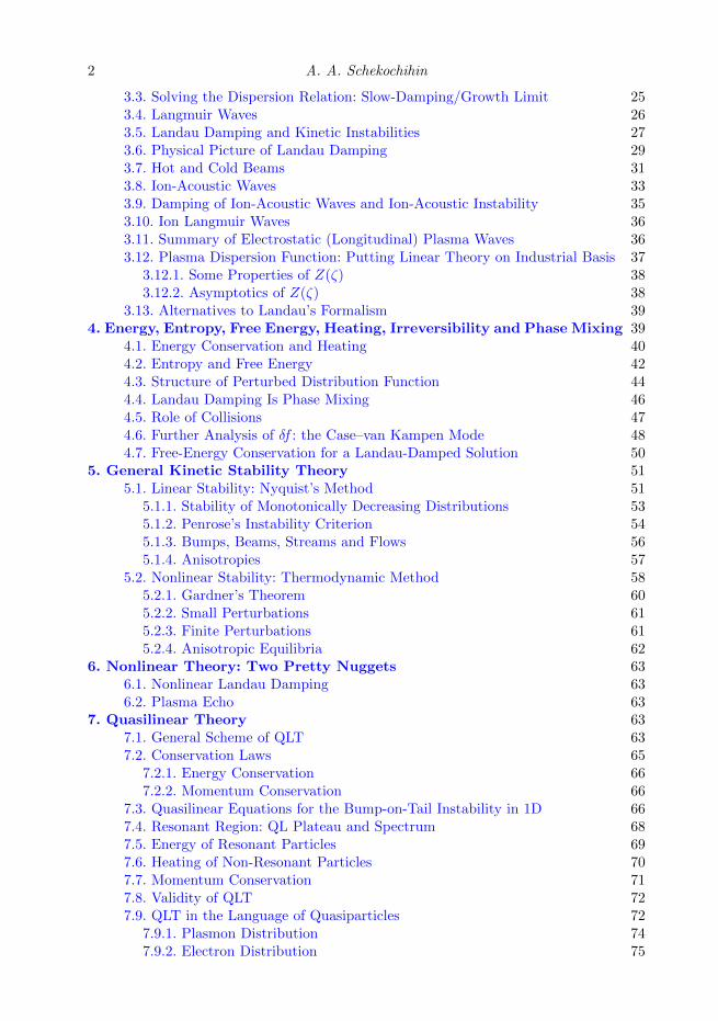
where the integral is along a straight line in the complex plane parallel to the imaginaryaxis and intersecting the real axis at Re p = σ (Fig. 4).
Since we expect to be able to recover our desired time-dependent function δf(v, t)from its Laplace transform, it is worth knowing the latter. To find it, we Laplace-transform (3.1):
l.h.s. =
∫ ∞0
dt e−pt∂δf
∂t=[e−ptδf
]∞0
+ p
∫ ∞0
dt e−ptδf = −g + p δf ,
r.h.s. = −ik · v δf +q
mϕ ik · ∂f0
∂v. (3.7)
Equating these two expressions, we find the solution:
δf(p) =1
p+ ik · v
[iq
mϕ(p)k · ∂f0
∂v+ g
]. (3.8)
Oxford MMathPhys Lectures: Plasma Kinetics and MHD 21
Figure 4. Layout of the complex-p plane: δf(p) is analytic for Re p > σ. At Re p < σ, δf(p)may have singularities (poles).
The Laplace transform of the potential, ϕ(p), itself depends on δf via (3.2):
ϕ(p) =
∫ ∞0
dt e−pt ϕ(t) =4π
k2
∑α
qα
∫d3v δfα(p)
=4π
k2
∑α
qα
∫d3v
1
p+ ik · v
[iqαmα
ϕ(p)k · ∂f0α
∂v+ gα
]. (3.9)
This is an algebraic equation for ϕ(p). Collecting terms, we get[1−
∑α
4πq2α
k2mαi
∫d3v
1
p+ ik · vk · ∂f0α
∂v
]︸ ︷︷ ︸
≡ ε(p,k)
ϕ(p) =4π
k2
∑α
qα
∫d3v
gαp+ ik · v
. (3.10)
The prefactor in the left-hand side, which I denote ε(p,k), is called the dielectric function,because it encodes all the self-consistent charge-density perturbations that plasma setsup in response to an electric field. This is going to be an important function, so let uswrite it out beautifully:
ε(p,k) = 1−∑α
ω2pα
k2
i
nα
∫d3v
1
p+ ik · vk · ∂f0α
∂v, (3.11)
where the plasma frequency of species α is defined by [cf. (2.2)]
ω2pα =
4πq2αnαmα
. (3.12)
The solution of (3.10) is
ϕ(p) =4π
k2ε(p,k)
∑α
qα
∫d3v
gαp+ ik · v
. (3.13)

22 A. A. Schekochihin
Figure 5. New contour for the inverse Laplace transform.
To calculate ϕ(t), we need to inverse-Laplace-transform ϕ: similarly to (3.6),
ϕ(t) =1
2πi
∫ i∞+σ
−i∞+σ
dp eptϕ(p). (3.14)
How do we do this integral? Recall that δf and, therefore, ϕ only exists (i.e., is finite)for Re p > σ, whereas at Re p < σ, it can have singularities, i.e., poles—let us call thempi, indexed by i. If we analytically continue ϕ(p) everywhere to Re p < σ except thosepoles, the result must have the form
ϕ(p) =∑i
cip− pi
+A(p), (3.15)
where ci are some coefficients (residues) and A(p) is the analytic part of the solution. Theintegration contour in (3.14) can be shifted to Re p → −∞ but with the proviso that itcannot cross the poles, as shown in Fig. 5 (this is proven by making a closed loop out ofthe old and the new contours, joining them at ±i∞, and noting that this loop encloses nopoles). Then the contributions to the integral from the vertical segments of the contourare exponentially small,12 the contributions from the segments leading towards and awayfrom the poles cancel, and the contributions from the circles around the poles can, byCauchy’s formula, be expressed in terms of the poles and residues:
ϕ(t) =∑i
ciepit . (3.16)
Thus, in the long-time limit, perturbations of the potential will evolve ∝ epit, where piare poles of ϕ(p). In general, pi = −iωi + γi, where ωi is a real frequency (giving wave-like behaviour of perturbations), γi < 0 represents damping and γi > 0 growth of theperturbations (instability).
12They are exponentially small in time as t → ∞ because the integrand of the inverse Laplace
transform (3.14) contains a factor of eRe pt, which decays faster than any of the “modes” in (3.16).If ϕ(p) does not grow too fast at large p, the integral along the vertical part of the contour mayalso vanish at any finite t, but that is not guaranteed in general: indeed, looking ahead to theexplicit expression (3.27) for ϕ(p), with the Landau prescription for analytic continuation toRe p < 0 analogous to (3.20), we see that ϕ(p) will contain a term ∝ Gα(ip/k), which can belarge at large Re p, e.g., if Gα(vz) is a Maxwellian.

Oxford MMathPhys Lectures: Plasma Kinetics and MHD 23
Going back to (3.13), we realise that the poles of ϕ(p) are zeros of the dielectricfunction:
ε(pi,k) = 0 ⇒ pi = pi(k) = −iωi(k) + γi(k). (3.17)
To find the wave frequencies ωi and the damping/growth rates γi, we must solve thisequation, which is called the plasma dispersion relation.
We are not particularly interested in what ci’s are, but they can be computed from the initialconditions, also via (3.13). The reason we are not particularly interested is that if we set upan initial perturbation with a given k and then wait long enough, only the fastest-growing or,failing growth, the slowest-damped mode will survive, with all others having exponentially smallamplitudes. Thus, a typical outcome of the linear theory is ϕ(t) oscillating at some frequencyand growing or decaying at some rate. Since this is a solution of a linear equation, the prefactorin front of the exponential can be scaled arbitrarily and so does not matter.
3.2. Calculating the Dielectric Function: the “Landau Prescription”
In order to be able to solve ε(p,k) = 0, we must learn how to calculate ε(p,k) for anygiven p and k. Before I wrote (3.15), I said that ϕ, given by (3.13), had to be analyticallycontinued to the entire complex plane from the area where its analyticity was guaranteed(Re p > σ), but I did not explain how this was to be done. In order to do it, we mustlearn how to calculate the velocity integral in (3.11)—if we want ε(p,k) and, therefore,its zeros pi—and also how to calculate the similar integral in (3.13) containing gα if wealso want the coefficients ci in (3.16).
First of all, let us turn these integrals into a 1D form. Given k, we can always choosethe z axis to be along k.13 Then∫
d3v1
p+ ik · vk · ∂f0
∂v=
∫dvz
1
p+ ikvzk
∂
∂vz
∫dvx
∫dvy f0(vx, vy, vz)︸ ︷︷ ︸≡ F (vz)
= −i∫ +∞
−∞dvz
F ′(vz)
vz − ip/k. (3.18)
Assuming, reasonably, that F ′(vz) is a nice (analytic) function everywhere, the integrandin (3.18) has one pole, vz = ip/k. When Re p > σ > 0, this pole is harmless because, inthe complex plane associated with the vz variable, it lies above the integration contour,which is the real axis, vz ∈ (−∞,+∞). We can think of analytically continuing the aboveintegral to Re p < σ as moving the pole vz = ip/k down, towards and below the realaxis. As long as Re p > 0, this can be done with impunity, in the sense that the polestays above the integration contour, and so the analytic continuation is simply the sameintegral (3.18), still along the real axis. However, if the pole moves so far down thatRe p = 0 or Re p < 0, we must deform the contour of integration in such a way as to keepthe pole always above it, as shown in Fig. 6. This is called the Landau prescription andthe contour thus deformed is called the Landau contour, CL.
Let us prove that this is indeed an analytic continuation, i.e., that the integral (3.18), adjustedto be along CL, is analytic for all values of p. Let us cut the Landau contour at vz = ±R andclose it in the upper half-plane with a semicircle CR of radius R such that R > σ/k (Fig. 7).Then, with integration running along the truncated CL and counterclockwise along CR, we get,
13NB: This means that in what follows, k > 0 by definition.

24 A. A. Schekochihin
(a) Re p > 0 (b) Re p = 0 (c) Re p < 0
Figure 6. The Landau prescription for the contour of integration in (3.18).
Figure 7. Proof of Landau’s prescription [see (3.19)].
by Cauchy’s formula,∫CL
dvzF ′(vz)
vz − ip/k+
∫CR
dvzF ′(vz)
vz − ip/k= 2πi F ′
(ip
k
). (3.19)
Since analyticity is guaranteed for Re p > σ, the integral along CR is analytic. The right-handside is also analytic, by assumption. Therefore, the integral along CL is analytic—this is theintegral along the Landau contour if we take R→∞.
With the Landau prescription, our integral is calculated as follows:
∫CL
dvzF ′(vz)
vz − ip/k=
∫ +∞
−∞dvz
F ′(vz)
vz − ip/kif Re p > 0,
P∫ +∞
−∞dvz
F ′(vz)
vz − ip/k+ iπF ′
(ip
k
)if Re p = 0,
∫ +∞
−∞dvz
F ′(vz)
vz − ip/k+ i2πF ′
(ip
k
)if Re p < 0,
(3.20)
where the integrals are again over the real axis and the imaginary bits come from thecontour making a half (when Re p = 0) or a full (when Re p < 0) circle around the pole.In the case of Re p = 0, or ip = ω, the integral along the real axis is formally divergentand so we take its principal value, defined as
P∫ +∞
−∞dvz
F ′(vz)
vz − ω/k= limε→0
[∫ ω/k−ε
−∞+
∫ +∞
ω/k+ε
]dvz
F ′(vz)
vz − ω/k. (3.21)

Oxford MMathPhys Lectures: Plasma Kinetics and MHD 25
The difference between (3.21) and the usual Lebesgue definition of an integral is that the latterwould be ∫ +∞
−∞dvz
F ′(vz)
vz − ω/k=
[limε1→0
∫ ω/k−ε1
−∞+ limε2→0
∫ +∞
ω/k+ε2
]dvz
F ′(vz)
vz − ω/k, (3.22)
and this, with, in general, ε1 6= ε2, diverges logarithmically, whereas in (3.21), the divergencesneatly cancel.
The Re p = 0 case in (3.20),∫CL
dvzF ′(vz)
vz − ω/k= P
∫ +∞
−∞dvz
F ′(vz)
vz − ω/k+ iπF ′
(ωk
), (3.23)
which tends to be of most use in analytical theory, is a particular instance of Plemelj’s formula:for a real ζ and a well-behaved function f (no poles on or near the real axis),
limε→+0
∫ +∞
−∞dx
f(x)
x− ζ ∓ iε = P∫ +∞
−∞dx
f(x)
x− ζ ± iπf(ζ), (3.24)
also sometimes written as
limε→+0
1
x− ζ ∓ iε = P 1
x− ζ ± iπδ(x− ζ), (3.25)
Finally, armed with Landau’s prescription, we are ready to calculate. The dielectricfunction (3.11) becomes
ε(p,k) = 1−∑α
ω2pα
k2
1
nα
∫CL
dvzF ′α(vz)
vz − ip/k(3.26)
and, analogously, our Laplace-transformed solution (3.13) becomes
ϕ(p) = − 4πi
k3ε(p,k)
∑α
qα
∫CL
dvzGα(vz)
vz − ip/k, (3.27)
where Gα(vz) =∫
dvx∫
dvy gα(vx, vy, vz).
3.3. Solving the Dispersion Relation: Slow-Damping/Growth Limit
A particularly analytically solvable and physically interesting case is one in which, forp = −iω + γ, γ ω (or, if ω = 0, γ kvthα), i.e., the case of slow damping or growth.In this limit, the dispersion relation (3.17) is
ε(p,k) ≈ ε(−iω,k) + iγ∂
∂ωε(−iω,k) = 0. (3.28)
Setting the imaginary part of (3.28) to zero gives us the growth/damping rate in termsof the real frequency:
γ = −Im ε(−iω,k)
[∂
∂ωRe ε(−iω,k)
]−1
. (3.29)
Setting the real part of (3.28) to zero gives the equation for the real frequency:
Re ε(−iω,k) = 0 . (3.30)
26 A. A. Schekochihin
Thus, we now only need ε(p,k) with p = −iω. Using (3.23), we get
Re ε = 1−∑α
ω2pα
k2
1
nαP∫
dvzF ′α(vz)
vz − ω/k, (3.31)
Im ε = −∑α
ω2pα
k2
π
nαF ′α
(ωk
). (3.32)
Let us consider a two-species plasma, consisting of electrons and a single species ofions. There will be two interesting limits:• “High-frequency” electron waves: ω kvthe, where vthe =
√2Te/me is the “thermal
speed” of the electrons;14 this limit will give us Langmuir waves (§3.4), slowly dampedor growing (§3.5).• “Low-frequency” ion waves: a particularly tractable limit will be that of “hot”
electrons and “cold” ions, viz., kvthe ω kvthi, where vthi =√
2Ti/mi is the “thermalspeed” of the ions; this limit will give us the sound (“ion-acoustic waves”; §3.8), whichalso can be damped or growing (§3.9).
3.4. Langmuir Waves
Consider the limitω
k vthe, (3.33)
i.e., the phase velocity of the waves is much greater than the typical velocity of a particlefrom the “thermal bulk” of the distribution. This means that in (3.31), we can expand invz ∼ vthe being small compared to ω/k (higher values of vz are cut off by the equilibriumdistribution function). Note that ω kvthe also implies ω kvthi because
vthi
vthe=
√TiTe
me
mi 1 (3.34)
as long as Ti/Te is not huge.15 Thus, (3.31) becomes
Re ε = 1 +∑α
ω2pα
k2
1
nα
k
ωP∫
dvz F′α(vz)
[1 +
kvzω
+
(kvzω
)2
+
(kvzω
)3
+ . . .
]
= 1 +∑α
ω2pα
kω
[1
nα
∫dvz F
′α(vz)︸ ︷︷ ︸
= 0
− kω
1
nα
∫dvz Fα(vz)︸ ︷︷ ︸= 1
− 2k2
ω2
1
nα
∫dvz vzFα(vz)︸ ︷︷ ︸
= 0
−3k3
ω3
1
nα
∫dvz v
2zFα(vz)︸ ︷︷ ︸
= v2thα/2
+ . . .
]
= 1−∑α
ω2pα
ω2
[1 +
3
2
k2v2thα
ω2+ . . .
], (3.35)
14This is a standard well-defined quantity for a Maxwellian equilibrium distribution
Fe(vz) = (ne/√π vthe) exp(−v2z/v2the), but if we wish to consider a non-Maxwellian Fe, let vthe be
a typical speed characterising the width of the equilibrium distribution, defined by, e.g., (3.36).15For hydrogen plasma,
√mi/me ≈ 42, the answer to the Ultimate Question of Life, Universe
and Everything (Adams 1979).

Oxford MMathPhys Lectures: Plasma Kinetics and MHD 27
where we have integrated by parts everywhere, assumed that there are no mean flows,〈vz〉 = 0, and, in the last term, used
〈v2z〉 =
v2thα
2, (3.36)
which is indeed the case for a Maxwellian Fα or, if Fα is not a Maxwellian, can be viewedas the definition of vthα.
The ion contribution to (3.35) is small because
ω2pi
ω2pe
=Zme
mi 1, (3.37)
so ions do not participate in this dynamics at all. Therefore, to lowest order, the dispersionrelation Re ε = 0 becomes
1−ω2
pe
ω2= 0 ⇒ ω2 = ω2
pe =4πe2neme
, (3.38)
the Tonks & Langmuir (1929) dispersion relation for what is known as Langmuir, orplasma, oscillations. This is the formal derivation of the result that we already had, onphysical grounds, in §2.1.
We can do a little better if we retain the (small) k-dependent term in (3.35):
Re ε ≈ 1−ω2
pe
ω2
(1 +
3
2
k2v2the
ω2︸ ︷︷ ︸use
ω2 ≈ ω2pe
)= 0 ⇒ ω2 ≈ ω2
pe(1 + 3k2λ2De) , (3.39)
where λDe = vthe/√
2ωpe =√Te/4πe2ne is the “electron Debye length” [cf. (1.6)].
Equation (3.39) is the Bohm & Gross (1949a) dispersion relation, describing an upgradeof the Langmuir oscillations to dispersive Langmuir waves, which have a non-zero groupvelocity (this effect is due to electron pressure: see Exercise 3.1).
Note that all this is only valid for ω kvthe, which we now see is equivalent to
kλDe 1. (3.40)
Exercise 3.1. Langmuir hydrodynamics.16 Starting from the linearised kinetic equationfor electrons and ignoring perturbations of the ion distribution function completely, work outthe fluid equations for electrons (i.e., the evolution equations for the electron density ne andvelocity ue) and show that you can recover the Langmuir waves (3.39) if you assume thatelectrons behave as a 1D adiabatic fluid (i.e., have the equation of state pen
−γe = const with
γ = 3). You can prove that they indeed do this by calculating their density and pressure directlyfrom the Landau solution for the perturbed distribution function (see §§4.3 and 4.6), ignoringresonant particles. The “hydrodynamic” description of Langmuir waves will reappear in §10.
3.5. Landau Damping and Kinetic Instabilities
Now let us calculate the damping rate of Langmuir waves using (3.29), (3.32)and (3.39):
∂Re ε
∂ω≈
2ω2pe
ω3, Im ε ≈ −
ω2pe
k2
π
neF ′e
(ωk
)⇒ γ ≈ π
2
ω3
k2
1
neF ′e
(ωk
), (3.41)
16This is based on the 2017 exam question.

28 A. A. Schekochihin
(a) ωF ′(ω/k) < 0: Landau damping (b) ωF ′(ω/k) > 0: instability
Figure 8. The Landau resonance (particle velocities equalling phase speed of the wave vz = ω/k)leads to damping of the wave if more particles lag just behind than overtake the wave and toinstability in the opposite case.
where ω is given by (3.39). Provided ωF ′(ω/k) < 0 (as would be the case, e.g., forany distribution monotonically decreasing with |vz|; see Fig. 8a), γ < 0 and so this isindeed a damping rate, the celebrated Landau damping (Landau 1946; it was confirmedexperimentally two decades later, by Malmberg & Wharton 1964).
The same theory also describes a class of kinetic instabilities: if ωF ′(ω/k) > 0, thenγ > 0, so perturbations grow exponentially with time. An iconic example is the bump-on-tail instability (Fig. 8b), which arises when a high-energy (vz vthe) electron beamis injected into a plasma17 and which we will study in great detail in §7.
We see that the damping or growth of plasma waves occurs via their interaction withthe particles whose velocities coincide with the phase velocity of the wave (“Landauresonance”). Because such particles are moving in phase with the wave, its electric fieldis stationary in their reference frame and so can do work on these particles, giving itsenergy to them (damping) or receiving energy from them (instability). In contrast, other,out-of-phase, particles experience no mean energy change over time because the fieldthat they “see” is oscillating. It turns out (§3.6) that the process works in the spirit ofsocialist redistrbution: the particles slightly lagging behind the wave will, on average,receive energy from it, damping the wave, whereas those overtaking the wave will havesome of their energy taken away, amplifying the wave. The condition ωF ′(ω/k) < 0corresponds to the stragglers being more numerous than the strivers, leading to netdamping; ωF ′(ω/k) > 0 implies the opposite, leading to an instability (which then leadsto flattening of the distribution; see §7).
Let us note again that these results are quantitatively valid only in the limit (3.33),or, equivalently, (3.40). It makes sense that damping should be slow (γ ω) in thelimit where the waves propagate much faster than the majority of the electrons (ω/k vthe) and so can interact only with a small number of particularly fast particles (for a
Maxwellian equilibrium distribution, it is an exponentially small number ∼ e−ω2/k2v2the).If, on the other hand, ω/k ∼ vthe, the waves interact with the majority population andthe damping should be strong: a priori, we might expect γ ∼ kvthe.
Landau damping became a cause celebre in the mathematics community and in the wider science
17Here we are dealing with the case of a “warm beam” (meaning that it has a finite width). Itturns out that there exists also another instability, leading to growth of perturbations with ω/kto the right of the bump’s peak, due to a different, “fluid” kind of resonance and possible evenfor “cold beams” (i.e., beams of particles that all have the same velocity): see §3.7.
Oxford MMathPhys Lectures: Plasma Kinetics and MHD 29
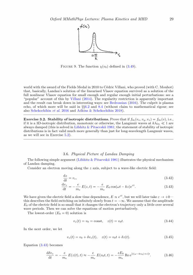
Figure 9. The function χ(v0) defined in (3.49).
world with the award of the Fields Medal in 2010 to Cedric Villani, who proved (with C. Mouhot)that, basically, Landau’s solution of the linearised Vlasov equation survived as a solution of thefull nonlinear Vlasov equation for small enough and regular enough initial perturbations: see a“popular” account of this by Villani (2014). The regularity restriction is apparently importantand the result can break down in interesting ways: see Bedrossian (2016). The culprit is plasmaecho, of which more will be said in §§6.2 and 8.4 (without claim to mathematical rigour; seealso Schekochihin et al. 2016 and Adkins & Schekochihin 2018).
Exercise 3.2. Stability of isotropic distributions. Prove that if f0e(vx, vy, vz) = f0e(v), i.e.,if it is a 3D-isotropic distribution, monotonic or otherwise, the Langmuir waves at kλDe 1 arealways damped (this is solved in Lifshitz & Pitaevskii 1981; the statement of stability of isotropicdistributions is in fact valid much more generally than just for long-wavelength Langmuir waves,as we will see in Exercise 5.2).
3.6. Physical Picture of Landau Damping
The following simple argument (Lifshitz & Pitaevskii 1981) illustrates the physical mechanismof Landau damping.
Consider an electron moving along the z axis, subject to a wave-like electric field:
dz
dt= vz, (3.42)
dvzdt
= − e
meE(z, t) = − e
meE0 cos(ωt− kz)eεt. (3.43)
We have given the electric field a slow time dependence, E ∝ eεt, but we will later take ε→ +0—this describes the field switching on infinitely slowly from t = −∞. We assume that the amplitudeE0 of the electric field is so small that it changes the electron’s trajectory only a little over severalwave periods. Then we can solve the equations of motion perturbatively.
The lowest-order (E0 = 0) solution is
vz(t) = v0 = const, z(t) = v0t. (3.44)
In the next order, we let
vz(t) = v0 + δvz(t), z(t) = v0t+ δz(t). (3.45)
Equation (3.43) becomes
dδvzdt
= − e
meE(z(t), t) ≈ − e
meE(v0t, t) = −eE0
meRe e[i(ω−kv0)+ε]t. (3.46)

30 A. A. Schekochihin
Integrating this gives
δvz(t) = −eE0
me
∫ t
0
dt′Re e[i(ω−kv0)+ε]t′
= −eE0
meRe
e[i(ω−kv0)+ε]t − 1
i(ω − kv0) + ε
= −eE0
me
εeεt cos[(ω − kv0)t]− ε+ (ω − kv0)eεt sin[(ω − kv0)t]
(ω − kv0)2 + ε2. (3.47)
Integrating again, we get
δz(t) =
∫ t
0
dt′ δvz(t′)
= −eE0
me
∫ t
0
dt′ Ree[i(ω−kv0)+ε]t
′− 1
i(ω − kv0) + ε
= −eE0
me
Re
e[i(ω−kv0)+ε]t − 1
[i(ω − kv0) + ε]2− εt
(ω − kv0)2 + ε2
= −eE0
me
[ε2 − (ω − kv0)2
] eεt cos[(ω − kv0)t]− 1
+ 2ε(ω − kv0)eεt sin[(ω − kv0)t]
[(ω − kv0)2 + ε2]2
− εt
(ω − kv0)2 + ε2
. (3.48)
The work done by the field on the electron per unit time, averaged over time, is the power gainedby the electron:
δP (v0) = −e 〈E(z(t), t)vz(t)〉
≈ −e⟨[E(v0t, t) + δz(t)
∂E
∂z(v0t, t)
][v0 + δvz(t)]
⟩= −eE0e
εt
⟨v0 cos[(ω − kv0)t]︸ ︷︷ ︸
vanishesunder
averaging
+ δvz(t) cos[(ω − kv0)t]︸ ︷︷ ︸only cos termfrom (3.47)
survivesaveraging
+ v0δz(t)k sin[(ω − kv0)t]︸ ︷︷ ︸only sin termfrom (3.48)
survivesaveraging
⟩
=e2E2
0
2mee2εt
ε
(ω − kv0)2 + ε2+
2kv0ε(ω − kv0)
[(ω − kv0)2 + ε2]2
=e2E2
0
2mee2εt
d
dv0
εv0(ω − kv0)2 + ε2︸ ︷︷ ︸≡ χ(v0)
. (3.49)
We see (Fig. 9) that—if the electron is lagging behind the wave, v0 . ω/k, then χ′(v0) > 0 ⇒ δP (v0) > 0, soenergy goes from the field to the electron (the wave is damped);—if the electron is overtaking the wave, v0 & ω/k, then χ′(v0) < 0 ⇒ δP (v0) < 0, so energygoes from the electron to the field (the wave is amplified).
Now remember that we have a whole distribution of these electrons, F (vz). So the total powerper unit volume going into (or out of) them is
P =
∫dvz F (vz)δP (vz) =
e2E20e
2εt
2me
∫dvz F (vz)χ
′(vz)
= −e2E2
0e2εt
2me
∫dvz F
′(vz)χ(vz). (3.50)

Oxford MMathPhys Lectures: Plasma Kinetics and MHD 31
Figure 10. Electron distribution with a cold beam; see (3.54).
Noticing that, by Plemelj’s formula (3.25), in the limit ε→ +0,
χ(vz) =εvz
(ω − kvz)2 + ε2= − ivz
2
(1
kvz − ω − iε− 1
kvz − ω + iε
)→ π
ω
k2δ(vz −
ω
k
), (3.51)
we conclude
P = − e2E20
2mek2πωF ′
(ωk
). (3.52)
As in §3.5, we find damping if ωF ′(ω/k) < 0 and instability if ωF ′(ω/k) > 0.Thus, around the wave-particle resonance vz = ω/k, the particles just lagging behind the
wave receive energy from the wave and those just overtaking it give up energy to it. Therefore,qualitatively, damping occurs if the former particles are more numerous than the latter. We seethat Landau’s mathematics in §§3.1–3.5 led us to a result that makes physical sense.
3.7. Hot and Cold Beams
Let us return to the unstable situation, when a high-energy beam produces a bump on thetail of the distribution function and thus electrostatic perturbations can suck energy out of thebeam and grow in the region of wave numbers where v0 < ω/k < ub. Here v0 is the point of theminimum of the distribution in Fig. 8(b) and ub is the point of the maximum of the bump, whichis the velocity of the beam; we are assuming that ub vthe. In view of (3.41), the instabilitywill have a greater growth rate if the bump’s slope is steeper, i.e., if the beam is colder (narrowerin vz space).
Imagine modelling the beam with a little Maxwellian distribution with mean velocity ub,tucked onto the bulk distribution:18
Fe(vz) =ne − nb√π vthe
exp
(− v2zv2the
)+
nb√π vb
exp
[− (vz − ub)2
v2b
], (3.53)
where nb is the density of the beam, vb is its width, and so Tb = mev2b/2 is its “temperature”,
just like Te = mev2the/2 is the temperature of the thermal bulk. A colder beam will have less
of a thermal spread around ub. It turns out that if the width of the beam is sufficiently small,another instability appears, whose origin is hydrodynamic rather than kinetic. In the interest ofhaving a full picture, let us work it out.
Consider a very simple limiting case of the distribution (3.53): let vb → 0 and nb ne. Then(Fig. 10)
Fe(vz) = FM(vz) + nbδ(vz − ub), (3.54)
where FM is the bulk Maxwellian from (3.53) (with density ≈ ne, neglecting nb in comparison).Let us substitute the distribution (3.54) into the dielectric function (3.26), seek solutions withp/k vthe, expand the part containing FM in the same way as we did in §3.4,19 neglect the
18The fact that we are working in 1D means that we are restricting our consideration toperturbations whose wave numbers k are parallel to the beam’s velocity. In general, allowingtransverse wave numbers brings into play the transverse (electromagnetic) part of the dielectrictensor (see Q2). However, for non-relativistic beams, the fastest-growing modes will still be thelongitudinal, electrostatic ones (see, e.g., Alexandrov et al. 1984, §32).19We can treat the Landau contour as simply running along the real axis because we are

32 A. A. Schekochihin
Figure 11. Sketch of the growth rate of the hydrodynamic and kinetic beam instabilities: see(3.57) for k < ωpe/ub, (3.58) for k = ωpe/ub, and (3.41) for ωpe/ub < k < ωpe/v0, where v0 isthe point of the minimum of the distribution in Fig. 8(b) and ub is the point of the maximumof the bump.
ion contribution for the same reason as we did there, and deal with the term in the dielectricfunction containing δ′(vz − ub) by integrating by parts. The resulting dispersion relation is
ε ≈ 1 +ω2pe
p2− nb
ne
ω2pe
(kub − ip)2= 0. (3.55)
Since nb ne, the last term can only matter for those perturbations that are close to resonancewith the beam (this is called the Cherenkov resonance):
p = −ikub + γ, γ kub. (3.56)
This turns (3.55) into
1−ω2pe
k2u2b
+nb
ne
ω2pe
γ2= 0 ⇒ γ = ±
√nb
ne
(1
k2u2b
− 1
ω2pe
)−1/2
. (3.57)
The expression under the square root is positive and so there is indeed a growing mode only ifk < ωpe/ub. This is in contrast to the case of a hot (or warm) beam in §3.5: there, having a kineticinstability required ωF ′e(ω/k) > 0, which was only possible at k > ωpe/ub (the phase speed ofthe perturbations had to be to the left of the bump’s maximum). The new instability thatwe have found—the hydrodynamic beam instability—has the largest growth rate at kub = ωpe,i.e., when the beam and the plasma oscillations are in resonance, in which case, to resolve thesingularity, we need to retain γ in the second term in (3.55). Doing so and expanding in γ,we get
ε ≈ 1−ω2pe
(ωpe + iγ)2+nb
ne
ω2pe
γ2≈ 2iγ
ωpe+nb
ne
ω2pe
γ2= 0 ⇒ γ =
(±√
3 + i
2,−i)(
nb
2ne
)1/3
ωpe .
(3.58)The unstable root (Re γ > 0) is the interesting one. The growth rate of the combined beaminstability, hydrodynamic and kinetic, is sketched in Fig. 11.
Exercise 3.3. This instability is called “hydrodynamic” because it can be derived from fluidequations (cf. Exercise 3.1) describing cold electrons (vthe = 0) and a cold beam (vb = 0).Convince yourself that this is the case.
Exercise 3.4. Using the model distribution (3.53), work out the conditions on vb and nb thatmust be satisfied in order for our derivation of the hydrodynamic beam instability to be valid,i.e., for (3.55) to be a good approximation to the true dispersion relation. What is the effect of
expecting to find a solution with Re p > 0 [see (3.20)], for reasons independent of the Landauresonance.

Oxford MMathPhys Lectures: Plasma Kinetics and MHD 33
(a) Cold streams: see (3.59) (b) Hot streams: see (5.16) and Q4
Figure 12. Two streams.
finite vb on the hydrodynamic instability? Sketch the growth rate of unstable perturbations asa function of k, taking into account both the hydrodynamic instability and the kinetic one, aswell as the Landau damping.
Exercise 3.5. Two-stream instability. This is a popular instability20 that arises, e.g., ina situation where the plasma consists of two cold counterstreams of electrons propagatingagainst a quasineutrality-enforcing background of effectively immobile ions (Fig. 12a). Modelthe corresponding electron distribution by
Fe(vz) =ne2
[δ(vz − ub) + δ(vz + ub)] (3.59)
and solve the resulting dispersion relation (where the ion terms can be neglected for thesame reason as in §3.4). Find the wave number at which perturbations grow fastest and thecorresponding growth rate. Find also the maximum wave number at which perturbations cangrow. If you want to know what happens when the two streams are warm (have a finite thermalspread vb; Fig. 12b), a nice fully tractable quantitative model of such a situation is the double-Lorentzian distribution (5.16). The dispersion relation for it can be solved exactly: this is donein Q4. You will again find a hydrodynamic instability, but is there also a kinetic one (due toLandau resonance)? It is an interesting and non-trivial question why not.
3.8. Ion-Acoustic Waves
Let us now see what happens at lower frequencies,
vthe ω
k vthi, (3.60)
i.e., when the waves propagate slower than the bulk of the electron distribution butfaster than the bulk of the ion one (Fig. 13). This is another regime in which we mightexpect to find weakly damped waves: they are out of phase with the majority of the ions,so F ′i (ω/k) might be small because Fi(ω/k) is small, while as far as the electrons areconcerned, the phase speed of the waves is deep in the core of the distribution, perhapsclose to its maximum at vz = 0 (if that is where its maximum is) and so F ′e(ω/k) mightturn out to be small because Fe(vz) changes slowly in that region.
To make this more specific, let us consider Maxwellian electrons:
Fe(vz) =ne√π vthe
exp
[− (vz − ue)2
v2the
], (3.61)
20It was discovered by engineers (Haeff 1949; Pierce & Hebenstreit 1949) and quickly adoptedby physicists (Bohm & Gross 1949b). Buneman (1958) realised that a case with an electron andan ion stream (i.e., with plasma carrying a current) is unstable in an analogous way. The kineticversion of the latter situation is the ion-acoustic instability derived in §3.9. In §5.1.3, we willdiscuss in a more general way the stability of distributions featuring streams.

34 A. A. Schekochihin
where we are, in general, allowing the electrons to have a mean flow (current). We willassume that ue vthe but allow ue ∼ ω/k. We can anticipate that this will give us aninteresting new effect. Indeed,
F ′e(vz) = −2(vz − ue)v2
the
Fe(vz). (3.62)
For resonant particles, vz = ω/k, the prefactor will be small, so we can hope for γ ω,as anticipated above, but note that its sign will depend on the relative size of ue andω/k and so we might (we will!) get an instability (§3.9).
But let us not get ahead of ourselves: we must first calculate the real frequency ω(k)of these waves, from (3.30) and (3.31):
Re ε = 1−ω2
pe
k2
1
neP∫
dvzF ′e(vz)
vz − ω/k−ω2
pi
k2
1
niP∫
dvzF ′i (vz)
vz − ω/k︸ ︷︷ ︸≈ω2pi
ω2
(1 + 3k2λ2
Di
)= 0. (3.63)
The last (ion) term in this equation can be expanded in kvz/ω 1 in exactly the sameway as it was done in (3.35). The expansion is valid provided
kλDi 1, (3.64)
and we will retain only the lowest-order term, dropping the k2λ2Di correction. The second
(electron) term in (3.63) is subject to the opposite limit, vz ω/k, so, using (3.62),
ω2pe
k2
1
neP∫
dvzF ′e(vz)
vz − ω/k≈ −
ω2pe
k2
1
neP∫
dvz2(vz − ue)v2
thevzFe(vz) ≈ −
2ω2pe
k2v2the
= − 1
k2λ2De
,
(3.65)where we have neglected ue vz because this integral is over the thermal bulk of theelectron distribution.
With all these approximations, (3.63) becomes
Re ε = 1 +1
k2λ2De
−ω2
pi
ω2= 0. (3.66)
The dispersion relation is then
ω2 =ω2
pi
1 + 1/k2λ2De
=k2c2s
1 + k2λ2De
, (3.67)
where
cs = ωpiλDe =
√ZTemi
(3.68)
is the sound speed, called that because, if we take kλDe 1, (3.67) describes a wave thatis very obviously a sound, or ion-acoustic, wave:
ω = ±kcs . (3.69)
The phase speed of this wave is the sound speed, ω/k = cs. That the expression (3.68)for cs combines electron temperature and ion mass is a hint as to the underlying physicsof sound propagation in plasma: ions provide the inertia, electrons the pressure (seeExercise 3.6).

Oxford MMathPhys Lectures: Plasma Kinetics and MHD 35
Figure 13. Ion-acoustic resonance: damping (cs > ue) or instability (cs < ue). Ion Landaudamping is weak because cs vthi, so in the tail of Fi(vz); electron damping/instability is alsoweak because ue, cs vthe, so close to the peak Fe(vz).
We can now check under what circumstances the condition (3.60) is indeed satisfied:
csvthe
=
√Zme
mi 1,
csvthi
=
√ZTeTi 1, (3.70)
with the latter condition requiring that the ions should be colder than the electrons.
Exercise 3.6. Hydrodynamics of sound waves. Starting from the linearised kinetic equa-tions for ions and electrons, work out the fluid equations for the plasma (i.e., the evolutionequations for its mass density and mass flow velocity). Assuming mi me and Ti Te, showthat the sound waves (3.69) with cs given by (3.68) are recovered if electrons have the equationof state of an isothermal fluid. Why should this be the case physically? Why is the equation ofstate for electrons different in a sound wave than in a Langmuir wave (see Exercise 3.1)? Wewill revisit ion hydrodynamics in §10.
3.9. Damping of Ion-Acoustic Waves and Ion-Acoustic Instability
Are ion acoustic waves damped? Can they grow? We have a standard protocol foranswering this question: calculate Re ε and Im ε and substitute into (3.29). Using (3.66)and (3.32), we find
∂Re ε
∂ω=
2ω2pi
ω3, Im ε = −
ω2pe
k2
π
neF ′e
(ωk
)−ω2
pi
k2
π
niF ′i
(ωk
). (3.71)
The two terms in Im ε represent the interaction between the waves and, respectively,electrons and ions. The ion term is small both on account of ωpi ωpe and, assumingMaxwellian ions, of the exponential smallness of Fi(ω/k) ∝ exp[−(ω/kvthi)
2]. We arethen left with
γ = − Im ε
∂(Re ε)/∂ω= −√π
ω3
k2v3the
mi
Zme
(ωk− ue
), (3.72)

36 A. A. Schekochihin
where we have used (3.62). In the long-wavelength limit, kλDe 1, we have ω = ±kcs,and so, for the “+” mode,
γ = −√πZme
8mik (cs − ue) . (3.73)
If the electron flow is subsonic, ue < cs, this describes the Landau damping of ion acousticwaves on hot electrons. If, on the other hand, the electron flow is supersonic, the signof γ reverses21 and we discover the ion-acoustic instability: excitation of ion acousticwaves by a fast electron current. The instability belongs to the same general class as,e.g., the bump-on-tail instability (§3.5) in that it involves waves sucking energy fromparticles, but the new conceptual feature here is that such energy conversion can resultfrom a collaboration between different particle species (electrons supplying the energy,ions carrying the wave).
There is a host of related instabilities involving various combinations of electron andion beams, currents, streams and counterstreams—excellent treatments of them can befound in the textbooks by Krall & Trivelpiece (1973) and by Alexandrov et al. (1984) orin the review by Davidson (1983). I shall return to this topic in §5.1.3.
Exercise 3.7. Damping of sound waves on ions.22 Find the ion contribution to the dampingof ion-acoustic waves. Under what conditions does it become comparable to, or larger than, theelectron contribution?
3.10. Ion Langmuir Waves
Note that since
λDe
λDi=vtheωpi
vthiωpe=
√ZTeTi
, (3.74)
the condition (3.64) need not entail kλDe 1 in the limit of cold ions [see (3.70)]—in thiscase, the size of the Debye sphere (1.6) is set by the ions, rather than by the electrons,and so we can have perfectly macroscopic (in the language of §1.4) perturbations onscales both larger and smaller than λDe. At larger scales, we have found sound waves(3.69). At smaller scales, kλDe 1, the dispersion relation (3.67) gives us ion Langmuiroscillations:
ω2 = ω2pi =
4πZ2e2nimi
, (3.75)
which are analogous to the electron Langmuir oscillations (3.38) and, like them, turn intodispersive ion Langmuir waves if the small k2λ2
Di correction in (3.63) is retained, leadingto the Bohm–Gross dispersion relation (3.39), but with ion quantities this time.
Exercise 3.8. Derive the dispersion relation for ion Langmuir waves. Investigate their damp-ing/instability.
3.11. Summary of Electrostatic (Longitudinal) Plasma Waves
We have achieved what turns out to be a basically complete characterisation ofelectrostatic (also known as “longitudinal”, in the sense that k ‖ E) waves in anunmagnetised plasma. These are summarised in Fig. 14. In the limit of short wavelengths,
21Recall that k > 0 by the choice of the z axis.22The 2016 exam question was loosely based on this.

Oxford MMathPhys Lectures: Plasma Kinetics and MHD 37
Figure 14. Electrostatic (longitudinal) plasma waves.
kλDe 1 and kλDi 1, the electron and ion branches, respectively, becomes dispersive,their damping rates increase and eventually stop being small. This corresponds to waveshaving phase speeds that are comparable to the speeds of the particles in the thermalbulk of their distributions, so a great number of particles are available to have Landauresonance with the waves and absorb their energy—the damping becomes strong.
Note that if the cold-ion condition Ti Te is not satisfied, the sound speed iscomparable to the ion thermal speed cs ∼ vthi, and so the ion-acoustic waves are stronglydamped at all wave numbers—it is well-nigh impossible to propagate sound through acollisionless hot plasma (no one will hear you scream)!
3.12. Plasma Dispersion Function: Putting Linear Theory on Industrial Basis
Clearly, we have entered the realm of practical calculation—it is now easy to imagine anindustry of solving the plasma dispersion relation
ε(p,k) = 1−∑α
ω2pα
k21
nα
∫CL
dvzF ′α(vz)
vz − ip/k= 0 (3.76)
and similar dispersion relations arising from, e.g., considering electromagnetic perturbations (seeQ2), magnetised plasmas (see Parra 2018b), different equilibria Fα (see Q3), etc.
A Maxwellian equilibrium is obviously an extremely important special case because that is,after all, the distribution towards which plasma is pushed by collisions on long time scales:
f0α(v) =nα
(πv2thα)3/2e−v
2/v2thα ⇒ Fα(vz) =nα√πvthα
e−v2z/v
2thα . (3.77)
For this case, we would like to introduce a new “special function” that would incorporate theLandau prescription for calculating the velocity integral in (3.76) and that we could in somesense “tabulate” once and for all.23
23In the olden days, one would literally tabulate it (Fried & Conte 1961). In the 21st century,we could just teach a computer to compute it [see (3.86)] and make an app.
38 A. A. Schekochihin
Taking Fα to be a Maxwellian and letting u = vz/vthα and ζα = ip/kvthα, we can rewrite thevelocity integral in (3.76) as follows
1
nα
∫CL
dvzF ′α(vz)
vz − ip/k= − 2√
π v2thα
∫CL
duu e−u
2
u− ζα= − 2
v2thα[1 + ζαZ(ζα)] , (3.78)
where the plasma dispersion function is defined to be
Z(ζ) =1√π
∫du
e−u2
u− ζ . (3.79)
In these terms, the plasma dispersion relation (3.76) becomes
ε = 1 +∑α
1 + ζαZ(ζα)
k2λ2Dα
= 0 . (3.80)
Note that if the Maxwellian distribution (3.77) has a mean flow, as it did, e.g., in (3.61), thisamounts to a shift by some mean velocity uα and all one needs to do to adjust the above resultsis to shift the argument of Z accordingly:
ζα → ζα −uαvthα
. (3.81)
3.12.1. Some Properties of Z(ζ)
It is not hard to see that
Z′(ζ) = − 1√π
∫du e−u
2 ∂
∂u
1
u− ζ = − 2√π
∫du
u e−u2
u− ζ = −2 [1 + ζZ(ζ)] . (3.82)
Let us treat this identity as a differential equation: the integrating factor is eζ2
, so
eζ2
Z(ζ) = −2
∫ ζ
0
dt et2
+ Z(0). (3.83)
We know the boundary condition at ζ = 0 from (3.23): for real ζ,
1√π
∫du
e−u2
u− ζ =1√πP∫ +∞
−∞du
e−u2
u− ζ︸ ︷︷ ︸= 0 for ζ = 0
becauseintegrand is
odd
+ i√π e−ζ
2
⇒ Z(0) = i√π. (3.84)
Using this in (3.83) and changing the integration variable t = −ix, we find
Z(ζ) = e−ζ2(i√π + 2i
∫ iζ
0
dx e−x2)
= 2i e−ζ2∫ iζ
−∞dx e−x
2
. (3.85)
This turns out to be a uniformly valid expression for Z(ζ): our function is simply a complex erf!Here is a Mathematica script for calculating it:
Z[zeta ] := I Sqrt[Pi] Exp[−zeta2](1 + I Erfi[zeta]). (3.86)
You can use this to code up (3.80) and explore, e.g., the strongly damped solutions (ζ ∼ 1,γ ∼ ω).
3.12.2. Asymptotics of Z(ζ)
If you believe in preserving the ancient art of asymptotic theory, you will find most useful(as, effectively, we did in §§3.4–3.9) various limiting forms of Z(ζ). At small argument |ζ| 1,

Oxford MMathPhys Lectures: Plasma Kinetics and MHD 39
the Taylor series is
Z(ζ) = i√π e−ζ
2
− 2ζ
(1− 2ζ2
3+
4ζ4
15− 8ζ6
105+ . . .
). (3.87)
At large argument, |ζ| 1, |Re ζ| |Im ζ|, the asymptotic series is
Z(ζ) = i√π e−ζ
2
− 1
ζ
(1 +
1
2ζ2+
3
4ζ4+
15
8ζ6+ . . .
). (3.88)
All the results (for a Maxwellian equilibrium) that I derived in §§3.4–3.10 can be readily obtainedfrom (3.80) by using the above limiting cases (see Q1). It is, indeed, a general practical strategyfor studying this and similar plasma dispersion relations to look for solutions in the limitsζα → 0 or ζα →∞, then check under what physical conditions the solutions thus obtained arevalid (i.e., that they indeed satisfy |ζα| 1 or |ζα| 1, |Re ζ| |Im ζ|), and then fill in thenon-asymptotic blanks in the same way that an experienced hunter espying antlers sticking outabove the shrubbery can reconstruct, in contour outline, the rest of the hiding deer.
Exercise 3.9. Work out the Taylor series (3.87). A useful step might be to prove this interestingformula (which also turns out to be handy in other calculations; see, e.g., Q8):
dmZ
dζm=
(−1)m√π
∫CL
duHm(u) e−u
2
u− ζ , (3.89)
where Hm(u) are Hermite polynomials [defined in (10.70)].
Exercise 3.10. Work out the asymptotic series (3.88) using the Landau prescription (3.20) andexpanding the principal-value integral similarly to the way it was done in (3.35). Work out also(or look up; e.g., Fried & Conte 1961) other asymptotic forms of Z(ζ), relaxing the condition|Re ζ| |Im ζ|.
3.13. Alternatives to Landau’s Formalism
Landau’s method of working out waves and damping in collisionless plasmas has a way elicitinga degree of dissatisfaction in the minds of some mathematically inclined people, and/or motivatesa search for alternatives. Perhaps the earliest and best known such alternative is the formalismdue to van Kampen. His objective was more mathematical rigour—but even if this is of limitedappeal to you, the book by van Kampen & Felderhof (1967) is still a good read and a goodchance to question and re-examine your understanding of how it all works.
Blithely skipping half a century of literature and focussing on the present, let me mentiona recent paper by Heninger & Morrison (2018), which, following up on Morrison (1994, 2000),recasts van Kampen’s scheme in terms of using a clever alternative transform, instead of theLaplace transform, to solve Landau’s initial-value problem.
You might find further enlightenment in another very recent paper, by Ramos & White (2018),where the Landau problem is recast as a proper eigenvalue problem—and it is shown, amongstother mathematical delights, that if one fiddles cleverly with initial conditions, one can obtainsolutions that do not decay at the Landau rate and, in fact, can have any time evolution thatone cares to specify!
4. Energy, Entropy, Free Energy, Heating, Irreversibility and PhaseMixing
While we are done with the “calculational” part of linear theory (calculating the ratesat which field perturbations oscillate, damp or grow), we are not yet done with the“conceptual” part: what exactly is going on, mathematically and physically? The planof addressing this question in this section is as follows.• I will show that Landau damping of perturbations of a plasma in thermal equilibrium

40 A. A. Schekochihin
leads to the heating of this equilibrium—basically, that energy is conserved. This is nota surprise, but it is useful to see explicitly how this works (§4.1).• I will then ask how it is possible to have heating (an irreversible process) in a plasma
that was assumed collisionless and must conserve entropy. In other words, why, physically,is Landau damping a damping? This will lead us to consider entropy evolution in oursystem and to introduce an important concept of free energy (§4.2).• In the above context, we will examine (§§4.3 and 4.6) the Laplace-transform solu-
tion (3.8) for the perturbed distribution function and establish the phenomenon of phasemixing—emergence of fine structure in velocity (phase) space. This will allow collisionsand, therefore, irreversiblity back in (§4.5). We will also see that the Landau-dampedsolutions are not eigenmodes (while growing solutions can be), and so conclude that itmade sense to insist on using an initial-value-problem formalism.
4.1. Energy Conservation and Heating
Let us go back to the full, nonlinear Vlasov–Poisson system, where we now restore thecollision term:
∂fα∂t
+ v ·∇fα −qαmα
(∇ϕ) · ∂fα∂v
=
(∂fα∂t
)c
, (4.1)
−∇2ϕ = 4π∑α
qα
∫d3v fα. (4.2)
Let us calculate the rate of change of the electric energy:
d
dt
∫d3r
E2
8π=
∫d3r
∇ϕ
4π· ∂(∇ϕ)
∂t︸ ︷︷ ︸by parts
= −∫
d3rϕ
4π
∂
∂t∇2ϕ︸ ︷︷ ︸
use (4.2)
=∑α
qα
∫∫d3r d3v ϕ
∂fα∂t︸ ︷︷ ︸
use (4.1)
=∑α
qα
∫∫d3r d3v ϕ
[−v ·∇fα︸ ︷︷ ︸by parts
+qαmα
(∇ϕ) · ∂f∂v︸ ︷︷ ︸
vanishesbecause
f(±∞) = 0
+
(∂fα∂t
)c︸ ︷︷ ︸
vanishesbecause
number ofparticles isconserved
]
=∑α
qα
∫∫d3r d3v fαv ·∇ϕ = −
∫d3rE · j, (4.3)
where j is the current density. So the rate of change of the electric field is minus the rateat which electric field does work on the charges, a.k.a. Joule heating—not a surprisingresult. The energy goes into accelerating particles, of course: the rate of change of their

Oxford MMathPhys Lectures: Plasma Kinetics and MHD 41
kinetic energy is
dK
dt=∑α
∫∫d3r d3v
mαv2
2
∂fα∂t︸ ︷︷ ︸
use (4.1)
=∑α
∫∫d3r d3v
m2α
2
[−v ·∇fα︸ ︷︷ ︸vanishesbecause
fulldivergence
+qαmα
(∇ϕ) · ∂fα∂v︸ ︷︷ ︸
by parts in v
+
(∂fα∂t
)c︸ ︷︷ ︸
vanishesbecauseenergy isconserved
]
= −∑α
qα
∫∫d3r d3v fαv ·∇ϕ =
∫d3rE · j. (4.4)
Combining (4.3) and (4.4) gives us the law of energy conservation:
d
dt
(K +
∫d3r
E2
8π
)= 0 . (4.5)
Exercise 4.1. Demonstrate energy conservation for the more general case in which magnetic-field perturbations are also allowed.
Thus, if the perturbations are damped, the energy of the particles must increase—thisis usually called heating. Strictly speaking, heating is a slow increase in the mean tem-perature of the thermal equilibrium. Let us make this statement quantitative. Considera Maxwellian plasma, homogeneous in space but possibly with some slow dependence ontime (cf. §2):
f0α =nα
(πv2thα)3/2
e−v2/v2thα = nα
(mα
2πTα
)3/2
e−mαv2/2Tα . (4.6)
In a homogeneous system with a fixed volume, the density nα is constant in timebecause the number of particles is constant: d(V nα)/dt = 0. We allow, however, that thetemperature may change: Tα = Tα(t). The total kinetic energy of the particles is
K = V∑α
∫d3v
mαv2
2f0α︸ ︷︷ ︸
=3
2nαTα
+∑α
∫∫d3r d3v
mαv2
2δfα. (4.7)
Let us average this over time, as per (2.7): the perturbed part vanishes and we have
〈K〉 = V∑α
3
2nαTα. (4.8)
Averaging also (4.5) and using (4.8), we get∑α
3
2nα
dTαdt
= − d
dt
1
V
∫d3r〈E2〉8π
, (4.9)
so the heating rate of the equilibrium equals the rate of decrease of the mean energy ofthe perturbations.

42 A. A. Schekochihin
We saw that the perturbations evolve according to (3.16). If we wait for a while, onlythe slowest-damped mode will matter, with all others exponentially small in comparison.Let us call its frequency and its damping rate ωk and γk < 0, respectively, so Ek ∝e−iωkt+γkt. If we assume that |γk| ωk, we may define the time average (2.7) in such away that ω−1
k ∆t |γk|−1. Then (4.9) becomes∑α
3
2nα
dTαdt
= −∑k
2γk|Ek|2
8π> 0 if γk < 0. (4.10)
The Landau damping rate of the electric-field perturbations is the heating rate of theequilibrium.24
This result, while at first glance utterly obvious, might, on reflection, appear to beparadoxical: surely, the heating of the equilibrium implies increasing entropy—but thedamping that is leading to the heating is collisionless and, in a collisionless system, inview of the H theorem, how can the entropy change?
4.2. Entropy and Free Energy
The kinetic entropy for each species of particles is defined to be
Sα = −∫∫
d3r d3v fα ln fα. (4.11)
This quantity [or, indeed, the full-phase-space integral of any quantity that is a functiononly of fα; see (5.26)] can only be changed by collisions and, furthermore, the plasma-physics version of Boltzmann’s H theorem says that
d
dt
∑α
Sα = −∑α
∫∫d3r d3v
(∂fα∂t
)c
ln fα > 0, (4.12)
where equality is achieved iff all fα are Maxwellian with the same temperature Tα = T .Thus, if collisions are ignored, the total entropy stays constant and everything that
happens is, in principle, reversible. So how can there be net damping of waves and,worse still, net heating of the equilibrium particle distribution?! Presumably, any dampingsolution can be turned into a growing solution by reversing all particle trajectories—soshould the overall perturbation level not stay constant?
As I already noted in §4.1, strictly speaking, heating is the increase of the equilibriumtemperature—and, therefore, of the equilibrium entropy. Indeed, for each species, theequilibrium entropy is
S0 = −∫∫
d3r d3v f0 ln f0 = −∫∫
d3r d3v f0
ln
[n(m
2π
)3/2]− 3
2lnT − mv2
2T
= V
[−n lnn
(m2π
)3/2
+3
2n lnT +
3
2n
], (4.13)
where we have used∫
d3v (mv2/2)f0 = (3/2)nT . Since n = const,
TdS0
dt= V
3
2n
dT
dt, (4.14)
so heating is indeed associated with the increase of S0.Since, according to (4.10), this can be successfully accomplished by collisionless damp-
ing and since entropy overall can only increase due to collisions, we must search for the
24Obviously, the damping of waves on particles of species α increases only the temperature ofthat species.

Oxford MMathPhys Lectures: Plasma Kinetics and MHD 43
“missing entropy” (or, rather, for the missing decrease of entropy) in the perturbed partof the distribution. The mean entropy associated with the perturbed distribution is
〈δS〉 = 〈S − S0〉 = −∫∫
d3r d3v 〈(f0 + δf) ln(f0 + δf)− f0 ln f0〉
= −∫∫
d3r d3v
⟨(f0 + δf)
[ln f0 +
δf
f0− δf2
2f20
+ . . .
]− f0 ln f0
⟩≈ −
∫∫d3r d3v
〈δf2〉2f0
, (4.15)
after expanding to second order in small δf/f0 and using 〈δf〉 = 0. The total entropy ofeach species, S = S0 + δS, can only by changed by collisions, so, if collisions are ignored,any heating of a given species, i.e., any increase in its S0 [see (4.14)] must be compensatedby a decrease in its δS. The latter can only be achieved by increasing 〈δf2〉: indeed, using(4.14) and (4.15), we find25
T
(dS0
dt+
d〈δS〉dt
)= V
3
2n
dT
dt− d
dt
∫∫d3r d3v
T 〈δf2〉2f0
= −∫∫
d3r d3v T
⟨(∂f
∂t
)c
ln f
⟩. (4.16)
If the right-hand side is ignored, T can only increase if 〈δf2〉 increases too.
It is useful to work out the collision term in (4.16) in terms of f0 and δf : using the fact that〈δf〉 = 0 by definition and that the number of particles is conserved by the collision operator,we get∫∫
d3r d3v T
⟨(∂f
∂t
)c
ln f
⟩≈∫∫
d3r d3v
[T
(∂f0∂t
)c
ln f0 +
⟨Tδf
f0
(∂δf
∂t
)c
⟩]= V
∫d3v
mv2
2
(∂f0∂t
)c
+
∫∫d3r d3v
⟨Tδf
f0
(∂δf
∂t
)c
⟩. (4.17)
The second term is the collisional damping of δf , of which more will be said soon. The first term isthe collisional energy exchange between the equilibrium distributions of different species (intra-species collisions conserve energy, but inter-species ones do not because there is friction betweenspecies). If the species under consideration is α, this energy exchange can be represented as∑α′ ναα′(Tα−Tα′) (see, e.g., Helander & Sigmar 2005) and will act to equilibrate temperatures
between species as the system strives toward thermal equilibrium. If the collision frequenciesναα′ are small, this will be a slow effect. Due to overall energy conservation, the energy-exchangeterms vanish exactly if (4.17) is summed over species.
Finally, let us sum (4.16) over species and use (4.9) to relate the total heating to the rateof change of the electric-perturbation energy:
d
dt
[∑α
∫∫d3r d3v
Tα〈δf2α〉
2f0α+
∫d3r〈E2〉8π
]︸ ︷︷ ︸
≡W
=∑α
∫∫d3r d3v
⟨Tαδfαf0α
(∂δfα∂t
)c
⟩6 0 ,
(4.18)where we used (4.17) in the right-hand side (with the total equilibrium collisional energy-exchange terms vanishing upon summation over species). The right-hand side must benon-positive-definite because collisions cannot decrease entropy [see (4.12)].
25In the second term, T can be brought inside the time derivative because 〈δf2〉/f0 f0.

44 A. A. Schekochihin
Equation (4.18) is a way to express the idea that, except for the effect of collisions, thechange in the electric-perturbation energy (= −heating) must be compensated by thechange in 〈δf2〉, in terms of a conservation law of a quadratic positive-definite quantity,W , that measures the total amount of perturbation in the system (a quadratic norm ofthe perturbed solution).26 It is not hard to realise that this quantity is the free energy ofthe perturbed state, comprising the entropy of the perturbed distribution and the energyof the electric field:
W = E −∑α
Tα〈δSα〉, E =
∫d3r〈E2〉8π
. (4.19)
It is quite a typical situation in non-equilibrium systems that there is an energy-like (quadratic inthe relevant fields and positive definite) quantity, which is conserved except for dissipation. Forexample, in hydrodynamics, the motions of a fluid are governed by the Navier–Stokes equation:
ρ
(∂u
∂t+ u ·∇u
)= −∇p+ µ∆u, (4.20)
where u is velocity, ρ mass density (ρ = const for an incompressible fluid), p pressure and µ thedynamical viscosity of the fluid. The conservation law is
d
dt
∫d3r
ρu2
2= −µ
∫d3r |∇u|2 6 0. (4.21)
The conserved quadratic quantity is kinetic energy and the negative-definite dissipation (leadingto net entropy production) is due to viscosity.27
Thus, as the electric perturbations decay via Landau damping, the perturbed distri-bution function must grow. This calls for going back to our solution for it (§3.1) andanalysing carefully the behaviour of δf .
4.3. Structure of Perturbed Distribution Function
Start with our solution (3.8) for δf(p) and substitute into it the solution (3.15) for ϕ(p):
δf(p) =1
p+ ik · v︸ ︷︷ ︸“kinetic”(ballistic)
pole
iq
m
[∑i
cip− pi︸ ︷︷ ︸
polesrepresenting
linearmodes, see
(3.17)
+ A(p)
]k · ∂f0
∂v+ g
. (4.22)
To compute the inverse Laplace transform (3.6), we adopt the same method as in §3.1(Fig. 5), viz., shift the integration contour to large negative Re p as shown in Fig. 15 and
26Note that the existence of such a quantity implies that the Maxwellian equilibrium is stable: if aquadratic norm of the perturbed solution cannot grow, clearly there cannot be any exponentiallygrowing solutions. This is known as Newcomb’s theorem, first communicated to the worldin the paper by Bernstein (1958, Appendix I). A generalisation of this principle to isotropicdistributions is the subject of Q6(c) and of §5.2.2, where the conserved quantity W will reemergein a different way, confirming its status as a Platonic entity that cannot be avoided.27You will find a similar conservation law for incompressible MHD if, in §11.11, you work out
the time evolution of∫
d3r (ρu2/2 +B2/8π) assuming ρ = const and ∇ · u = 0.

Oxford MMathPhys Lectures: Plasma Kinetics and MHD 45
Figure 15. Shifting the integration contour in (4.23). This is analogous to Fig. 5 but note theadditional “kinetic” pole.
use Cauchy’s formula:28
δf(t) =1
2πi
∫ i∞+σ
−i∞+σ
dp eptδf(p) = iq
m
∑i
ciepit
pi + ik · vk · ∂f0
∂v︸ ︷︷ ︸eigenmode-like
solution, comes fromthe poles of ϕ(p)
+ e−ik·vt
g − i q
m
[∑i
cipi + ik · v
+A(−ik · v)
]k · ∂f0
∂v
︸ ︷︷ ︸
ballistic response,comes fromp = −ik · v
. (4.23)
The solution (4.23) teaches us two important things.
1) First, the Landau-damped solution is not an eigenmode. Even though the evolutionof the potential, given by (3.16), does look like a sum of damped eigenmodes of the formϕ ∝ epit, Re pi < 0, the full solution of the Vlasov–Poisson system does not decay: thereis a part of δf(t), the “ballistic response” ∝ e−ik·vt, that oscillates without decaying—in fact, we shall see in §4.6 that δf even has a growing part! It is this part that isresponsible for keeping free energy conserved, as per (4.18) without collisions. Thus,you may think of Landau damping as a process of transferring (free) energy from theelectric-field perturbations to the perturbations of the distribution function.
28A perceptive reader has spotted that that this formula does not seem to satisfy δf(t = 0) = gunless A(−ik · v) = 0. This is because, as explained in fotnote 12, the method for calculatingthe inverse Laplace transform that involves discarding the integral along the vertical part ofthe shifted contour in Fig. 15 only works in the limit of long times. It is an amusing exercisein complex analysis to show that, in the (overly restrictive) case of ϕ(p) decaying quickly atRe p→ −∞, the solution (4.23) is also valid at finite t and, accordingly, A(−ik · v) = 0 (i.e., Avanishes for any purely imaginary p).

46 A. A. Schekochihin
Figure 16. Shearing of δf in phase space.
In contrast to the case of damping, a growing solution (Re pi > 0) can be viewed as an eigenmodebecause, after a few growth times, the first term in (4.23) will be exponentially larger than theballistic term. This will allow us to ignore the latter in our treatment of QLT (§7.1)—a handy,although not necessary (see Q9), simplification. Note that reversibility is not an issue for thegrowing solutions: so, there may be (and often are) damped solutions as well, so what? We onlycare about the growing modes because they will be all that is left if we wait long enough.
2) Secondly, the δf perturbations have fine structure in velocity (phase) space. Thisstructure gets finer with time: roughly speaking, if δf ∝ e−ikvt, then
1
δf
∂δf
∂v∼ ikt→∞ as t→∞. (4.24)
This phenomenon is called phase mixing. You can think of the basic mechanism respon-sible for it as a shearing in phase space: the homogeneous part of the linearised kineticequation,
∂δf
∂t+ v
∂δf
∂z= . . . , (4.25)
describes advection of δf by a linear shear flow in the the (z, v) plane. This turns any δfstructure in this plane into long thin filaments, with large gradients in v (Fig. 16).
4.4. Landau Damping Is Phase Mixing
Phase mixing helps us make sense of the notion that, even though ϕ is the velocityintegral of δf , the former can be decaying while the latter is not:
ϕ =4π
k2
∑α
qα
∫d3v δfα︸ ︷︷ ︸fine
structurecancels
∝ e−γt → 0. (4.26)
The velocity integral over the fine structure increasingly cancels as time goes on—aperturbation initially “visible” as ϕ phase-mixes away, disappearing into the negativeentropy associated with the fine velocity dependence of δf [see (4.15)].
More generally speaking, one can similarly argue that the refinement of velocitydependence of δf causes lower velocity moments of δf (density, flow velocity, pressure,heat flux, and so on) to decrease with time, transferring free energy to higher moments(ever higher as time goes on). One way to formalise this statement neatly is in termsof Hermite moments: since Hermite polynomials are orthogonal, the free energy of theperturbed distribution can be written as a sum of “energies” of the Hermite moments[see (10.73)]. It is then possible to represent the Landau-damped perturbations as havinga broad spectrum in Hermite space, with the majority of the free energy residing in
Oxford MMathPhys Lectures: Plasma Kinetics and MHD 47
high-order moments—infinitely high in the formal limit of zero collisionality and infinitetime (see Q8 and Kanekar et al. 2015).
Since the mth-order Hermite moment can, for m 1, be asymptotically represented as a cosinefunction in v space oscillating with the “frequency”
√2m/vth [see (10.74)], (4.24) implies that
the typical order of the moment in which the free energy resides grows with time as m ∼ (kvtht)2.
Taking Hermite (or other kind of) moments of the kinetic equation is essentially theprocedure for deriving “fluid” equations for the plasma—or, rather, plasma becomes afluid if this procedure can be stopped after a few moments (e.g., in the limit of strongcollisionality, this happens at the third moment; see Dellar 2015 and Parra 2018a). SinceLandau damping is a long-time effect of this phase-mixing process, it cannot be capturedby any fluid approximation to the kinetic system involving a truncation of the hierarchyof moment equations at some finite-order moment—it is an essentially kinetic effect“beyond all orders”.29
4.5. Role of Collisions
As ever larger velocity-space gradients emerge, it becomes inevitable that at some pointthey will become so large that collisions can no longer be ignored. Indeed, the Landaucollision operator is a Fokker–Planck (diffusion) operator in velocity space [see (1.36)]and so it will eventually wipe out the fine structure in v, however small is the collisionfrequency ν. Let us estimate how long this takes.
The size of the velocity-space gradients of δf due to ballistic response is given by (4.24).Then the collision term is(
∂δf
∂t
)c
∼ νv2th
∂2δf
∂v2∼ −νv2
thk2t2δf. (4.27)
Solving for the time evolution of the perturbed distribution function due to collisions,we get
∂δf
∂t∼ −ν(kvtht)
2δf ⇒ δf ∼ exp
(−1
3νk2v2
tht3
)≡ e−(t/tc)3 . (4.28)
Therefore, the characteristic collisional decay time is
tc ∼1
ν1/3(kvth)2/3. (4.29)
Note that tc ν−1 provided ν kvth, i.e., tc is within the range of times over which our“collisionless” theory is valid. After time tc, “collisionless” damping becomes irreversiblebecause the part of δf that is fast-varying in velocity space is lost (entropy has grown)and so it is no longer possible, even in principle, to invert all particle trajectories,have the system retrace back its steps, “phase-unmix” and thus “undamp” the dampedperturbation.
In a sufficiently collisionless system, phase unmixing is, in fact, possible if nonlinearity is
29One useful way to see this is by examining the structure of Langmuir hydrodynamics,which was the subject of Exercise 3.1. The moment hierarchy can be truncated by assumingkvthe/ω 1, but one can never capture Landau damping however many moments onekeeps: indeed, the Landau damping rate (3.41) for, say, a Maxwellian plasma will beγ ∝ exp(−ω2/k2v2the), all coefficients in the Taylor expansion of which in powers of kvthe/ωare zero.

48 A. A. Schekochihin
Figure 17. Coarse graining of the distribution function.
allowed—giving rise to the beautiful phenomenon of plasma echo, in which perturbations can firstappear to be damped away but then come back from phase space (§6.2). This effect is a source ofmuch preoccupation to pure mathematicians (Villani 2014; Bedrossian 2016): indeed the validityof the linearised Vlasov equation (3.1) as a sensible approximation to the full nonlinear one(2.12) is in question if the velocity derivative ∂δf/∂v in the last term of the latter starts growinguncontrollably. Phase unmixing has also recently turned out to have interesting consequencesfor the role of Landau damping in plasma turbulence (Schekochihin et al. 2016; Adkins &Schekochihin 2018).
Some rather purist theoreticians sometimes choose to replace collisional estimates of the typediscussed above by a stipulation that δf(v) must be “coarse-grained” beyond some suitablychosen scale in v (Fig. 17)—this is equivalent to saying that the formation of the fine-structuredphase-space part of δf constitutes a loss of information and so leads to growth of entropy (i.e.,the loss of negative entropy associated with 〈δf2〉). Somewhat non-rigorously, this means that wecan just consider the ballistic term in (4.23) to have been wiped out and use the coarse-grained(i.e., velocity-space-averaged) version of δf :30
δf = iq
m
∑i
ciepit
pi + ik · v k ·∂f0∂v
. (4.30)
We can check that the correct solution (3.16) for the potential can be recovered from this:
ϕ =4π
k2
∑α
qα
∫d3v δfα
=∑i
ciepit
[∑α
i4πq2αmαk2
∫d3v
1
pi + ik · v k ·∂f0α∂v− 1︸ ︷︷ ︸
= −ε(pi,k) = 0 by definition of pi
+1
]=∑i
ciepit. (4.31)
If you are wondering how this works without the coarse-graining kludge, read on.
4.6. Further Analysis of δf : the Case–van Kampen Mode
Having given a rather qualitative analysis of the structure and consequences of thesolution (4.23), I anticipate a degree of dissatisfaction from a perceptive reader. Yes,there is a non-decaying piece of δf . But conservation of free energy in a collisionlesssystem in the face of Landau damping in fact requires 〈δf2〉 to grow, not just to fail todecay [see (4.18)]. How do we see that this does indeed happen? The analysis that followsaddresses this question. These considerations are not really necessary for most practical
30With an understanding that any integral involving the resonant denominator must be takenalong the Landau contour (see Q9). If you adopt this shorthand, you can, nonrigorously butoften expeditiously, use Fourier transforms into frequency space, rather than Laplace transforms.

Oxford MMathPhys Lectures: Plasma Kinetics and MHD 49
Figure 18. Emergence of the Case–van Kampen mode.
plasma-physics calculations (see, however, Q9), but it may be necessary for your pieceof mind and comfort with this whole conceptual framework.
Let us rearrange the solution (4.23) as follows:
δf(t) = iq
m
∑i
ciepit − e−ik·vt
pi + ik · vk · ∂f0
∂v+ (g + . . . )e−ik·vt . (4.32)
The second term is the ballistic evolution of perturbations (particles flying apart instraight lines at different velocities)—a homogeneous solution of the kinetic equation(3.1). This develops a lot of fine-scale velocity-space structure, but obviously doesnot grow. The first term, a particular solution arising from the (linear) wave-particleinteraction, is more interesting, especially around the resonances Re pi + k · v = 0.
Consider one of the modes, pi = −iω + γ, and assume γ k · v ∼ ω. This allows usto introduce “intermediate” times:
1
k · v t 1
γ. (4.33)
This means that the wave has had time to oscillate, phase mixing has got underway,but the perturbation has not yet been damped away completely. We have then, for therelevant piece of the perturbed distribution (4.32),
δf ∝ epit − e−ik·vt
pi + ik · v= −ie−iωt e
γt − e−i(k·v−ω)t
k · v − ω − iγ≈ −ie−iωt 1− e
−i(k·v−ω)t
k · v − ω, (4.34)
with the last, approximate, expression valid at the intermediate times (4.33), assumingalso that, even though we might be close to the resonance, we shall not come closer thanγ, viz., |k · v − ω| γ. Respecting this ordering, but taking |k · v − ω| 1/t, we find
δf ∝ t e−iωt. (4.35)
Thus, δf has a peak that grows with time, emerging from the sea of fine-scale but constant-amplitude structures (Fig. 18). The width of this peak is obviously |k · v − ω| ∼ 1/t andso δf around the resonance develops a sharp structure, which, in the formal limit t→∞(but respecting γt 1, i.e., with infinitesimal damping), tends to a delta function:
δf ∝ −ie−iωt 1− e−i(k·v−ω)t
k · v − ω→ e−iωtπδ(k · v − ω) as t→∞. (4.36)

50 A. A. Schekochihin
Here is a “formal” proof:
1− e−ixt
x=
1− cosxt
x︸ ︷︷ ︸finite ast→∞,even atx = 0
+ isinxt
x︸ ︷︷ ︸= it atx = 0,
so dom-inant
≈ eixt − e−ixt
2x=i
2
∫ t
−tdt′eixt
′→ iπδ(x) as t→∞.
(4.37)The delta-function solution (4.36) is an instance of a Case–van Kampen mode (van Kam-pen 1955; Case 1959)—an object that belongs to the mathematical realms briefly alludedto in §3.13. Note that writing the solution in the vicinity of the resonance in this formis tantamount to stipulating that any integral taken with respect to v (or k) andinvolving δf must always be done along the Landau contour, circumventing the polefrom below [cf. (3.23)]. We will find the representation (4.36) of δf useful in working outthe quasilinear theory of Landau damping (in Q9).
If we restore finite damping, all this goes on until t ∼ 1/γ, with the delta functionreaching the height ∝ 1/γ and width ∝ γ. In the limit t 1/γ, the damped part of thesolution decays, eγt → 0, and we are left with just the ballistic part, the second termin (4.23).
4.7. Free-Energy Conservation for a Landau-Damped Solution
Finally, let us convince ourselves that, if we ignore collisions, we can recover (4.18) with a zeroright-hand side from the full collisionless Landau-damped solution given by (3.16) and (4.32).For simplicity, let us consider the case of electron Langmuir waves and prove that
d
dt
∫d3v
T |δfk|2
2f0= − d
dt
|Ek|2
8π= −2γk
|Ek|2
8π. (4.38)
Ignoring the term in (4.32) that involves g as it obviously cannot give us a growing amplitude,letting the relevant root of the dispersion relation be pi = −iωpe + γk, where γk is givenby Eq. (3.41), and assuming a Maxwellian f0, we may write the solution (4.32) for electrons(q = −e) as
δfk ≈e
mecie
pit︸ ︷︷ ︸= ϕk
1− e−i(k·v−ipi)t
k · v − ipi2k · vv2the
f0 ≈eϕk
Tk · v 1− e−i(k·v−ωpe)t
k · v − ωpe︸ ︷︷ ︸≈ iπδ(k ·v−ωpe)
f0. (4.39)
We are going to have to compute |δfk|2 and squaring delta functions is a dangerous gamebelonging to the class of games that one must play veeery carefully. Here is how:
∂
∂t
∣∣∣∣1− e−ixtx
∣∣∣∣2 =∂
∂t
4
x2sin2 xt
2=
2 sinxt
x−−−→t→∞
2πδ(x) ⇒∣∣∣∣1− e−ixtx
∣∣∣∣2 −−−→t→∞2πtδ(x).
(4.40)Using this prescription,∫
d3vT |δfk|2
2f0=
∫d3v
e2|ϕk|2
mev2the(k · v)22πtδ(k · v − ωpe)f0
= 2tk2|ϕk|2
8π
ω4pe
k3π
nev2theF(ωpe
k
)︸ ︷︷ ︸
= −γk > 0; see (3.41)
= −2γkt|Ek|2
8π. (4.41)
Thus, the entropic part of the free energy grows secularly with time and its time derivativesatisfies (4.38), q.e.d.

Oxford MMathPhys Lectures: Plasma Kinetics and MHD 51
5. General Kinetic Stability TheoryIn §3, we learned how to perturb some given equilibrium distribution f0α infinitesimally and
find the evolution of the perturbation: damping, growth, oscillation (as well as the interestingphase-space happenings that came to light in §4). Let us now pose the question in a more generalway. In a collisionless plasma, there can be infinitely many possible equilibria, including quitecomplicated ones. If we set one up, will it persist, i.e., is it stable? If it is not stable, whatmodification do we expect it to undergo in order to become stable? Other than solving thedispersion relation (3.17) to answer the first question and developing various types of nonlineartheories to answer the second (along the lines advertised in §2.4 and developed in §7 andsubsequent sections), both of which can be quite complicated and often intractable technicalchallenges, do we have at our disposal any general principles that allow us to pronounce onstability, linear or otherwise? Is there a general insight that we can cultivate as to what sort ofdistributions are likely to be stable or unstable and to what sorts of perturbations?
We have had glimpses of such general principles already. For example, in §3.5, we ascertained,by explicit calculation, that we could encounter a situation with a (small) growth rate if theequilibrium distribution had a positive derivative somewhere along the direction (z) of the wavenumber of the perturbation, viz., vzF
′e(vz) > 0. We developed this further in §3.7, finding
that not only hot but also cold beams and streams triggered instabities. In Exercise 3.2, Idropped a hint that general statements could perhaps be made about certain general classes ofdistributions: 3D-isotropic equilibria are stable (we shall prove this shortly). In Q6, we found thatisotropic, monotonically decreasing equilibria are stable not just against infinitesimal (linear),electrostatic perturbations, but also against small but finite electromagnetic ones, giving us ataste of a powerful nonlinear constraint. How general are these statements? Are they sufficientor also necessary criteria? Is there a universal stability litmus test? Let us attack the problemof kinetic stability with an aspiration to generality (although still, for now, for electrostaticperturbations only).
5.1. Linear Stability: Nyquist’s Method
We start with the relatively modest ambition to determine linear stability of generic equilibria,i.e., their stability against infinitesimal perturbations. This comes down to the question ofwhether the dispersion relation (3.17) has any unstable solutions: roots with growth ratesγi(k) > 0.
It is going to be useful to write the dielectric function (3.26) as follows
ε(p,k) = 1−ω2pe
k2
∫CL
dvzF ′(vz)
vz − ip/k, (5.1)
F =1
ne
∑α
Z2αme
mαFα =
Fene
+Zme
mi
Fini, (5.2)
where the last expression in (5.2) is for the case of a two-species plasma. Thus, the distributionfunctions of different species come into the linear problem additively, weighted by their species’charges and (inverse) masses.
Let us develop a method (due to Nyquist 1932) for counting zeros of ε(p) (we will henceforthsuppress k in the argument) in the half-plane Re p > 0 (the unstable roots of the dispersionrelation). We observe that ε(p) is analytic (be virtue of our efforts in §3.2 to make it so) andthat if p = pi is its zero of order Ni, then in its vicinity,
ε(p) = const (p− pi)Ni + . . . ⇒ ∂ ln ε(p)
∂p=
Nip− pi
+ . . . , (5.3)
so zeros of ε are poles of ∂ ln ε(p)/∂p; the latter function has no other poles because ε is analytic.If we now integrate this function over a closed contour CR running along the imaginary axis(and just to the right of it: p = −iω+ 0) in the complex p plane from iR to −iR and then alonga semicircle of radius R back to iR (Fig. 19), we will, in the limit R → ∞, capture all these

52 A. A. Schekochihin
Figure 19. Integration contour for (5.4).
poles:
limR→∞
∫CR
dp∂ ln ε(p)
∂p= 2πi
∑i
Ni = 2πiN, (5.4)
where N is the total number of zeros of ε(p) in the half-plane Re p > 0. It turns out (as we shallprove in a moment) that the contribution to the integral over CR from the semicircle vanishesat R→∞ and so we need only integrate along the imaginary axis:
2πiN =
∫ −i∞+0
+i∞+0
dp∂ ln ε(p)
∂p= ln
ε(−i∞)
ε(+i∞). (5.5)
Proof. All we need to show is that
|p|∂ ln ε(p)
∂p→ 0 as |p| → ∞, Re p > 0. (5.6)
Indeed, using (5.1) and the Landau integration rule (3.20), we have in this limit:
ε(p) = 1−ω2pe
k2
∫ +∞
−∞dvz F
′(vz)ik
p
(1− ikvz
p+ . . .
)≈ 1 +
1
p2
∑α
ω2pα, (5.7)
where we have integrated by parts and used∫
dvz Fα = nα. Manifestly, the condition (5.6) issatisfied.
Note that, along the imaginary axis p = −iω, by the same expansion and using also thePlemelj formula (3.23), we have
ε(−iω) ≈ 1− 1
ω2
∑α
ω2pα − iπ
ω2pe
k2F ′(ωk
)→ 1∓ i0 as ω → ∓∞. (5.8)
This is going to be useful shortly.
In view of (5.8) and of our newly proven formula (5.5), as the function ε(−iω) runs along thereal line in ω, it changes from
ε(i∞) = 1− i0 at ω = −∞, (5.9)
where we have arbitrarily fixed its phase, to
ε(−i∞) = e2πiN + i0 at ω = +∞, (5.10)
where N is the number of times the function
ε(−iω) = 1−ω2pe
k2
[P∫ +∞
−∞dvz
F ′(vz)
vz − ω/k+ iπF ′
(ωk
)](5.11)

Oxford MMathPhys Lectures: Plasma Kinetics and MHD 53
(a) Single-maximum, stable equilibrium (b) Strange but stable equilibrium
Figure 20. Two examples of Nyquist diagrams showing stability (because failing to circle zero):(a) the case of a monotonically decreasing distribution (§5.1.1, Fig. 21a); (b) another stable case,even though very complicated (it also illustrates the argument in §5.1.2).
circles around the origin in the complex ε plane. Since N is also the number of unstable rootsof the dispersion relation, this gives us a way to count these roots by sketching ε(−iω)—thissketch is called the Nyquist diagram. Two examples of Nyquist diagrams implying stability aregiven in Fig. 20: the curve ε(−iω) departs from 1− i0 and comes back to 1 + i0 via a path that,however complicated, never makes a full circle around zero. Two examples of unstable situationsappear in Fig. 22(b,d): in these cases, zero is circumnavigated, implying that the equilibriumdistribution F is unstable (at a given value of k).
In order to work out whether the Nyquist curve circles zero (and how many times), all oneneeds to do is find Re ε(−iω) at all points ω where Im ε(−iω) = 0, i.e., where the curve intersectsthe real line, and hence sketch the Nyquist diagram. We shall see in a moment, with the aid ofsome important examples, how this is done, but let us do a little bit of preparatory work first.
It follows immediately from (5.11) that these crossings happen whenever ω/k = v∗ is a velocityat which F (vz) has an extremum, F ′(v∗) = 0. At these points, the dielectric function (5.11) isreal and can be expressed so:
ε(−ikv∗) = 1 +ω2pe
k2P (v∗) . (5.12)
Here P (v∗) is (minus) the principal-value integral in (5.11), which can be manipulated as follows:
P (v∗) = −P∫ +∞
−∞dvz
F ′(vz)
vz − v∗= −P
∫ +∞
−∞dvz
1
vz − v∗∂
∂vz
[F (vz)− F (v∗)
]=
∫ +∞
−∞dvz
F (v∗)− F (vz)
(vz − v∗)2, (5.13)
where we have integrated by parts; the additional term F (v∗) was inserted under the derivativein order to eliminate the boundary terms arising in this integration by parts around the polevz = v∗.
31
Now we are ready to analyse particular (and, as we shall see, also generic) equilibriumdistributions F (vz).
5.1.1. Stability of Monotonically Decreasing Distributions
Consider first a distribution function that has a single maximum at vz = v0 and monotonicallydecays in both directions away from it (Fig. 21a): F ′(v0) = 0, F ′′(v0) < 0. This means that,
31Note that in the final expression in (5.13), there is no longer a need for principal-value
integration because, v∗ being a point of extremum of F , the numerator of the integrand isquadratic in vz − v∗ in the vicinity of v∗.
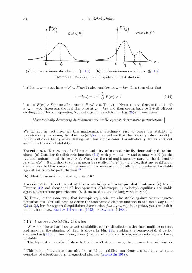
54 A. A. Schekochihin
(a) Single-maximum distribution (§5.1.1) (b) Single-minimum distribution (§5.1.2)
Figure 21. Two examples of equilibrium distributions.
besides at ω = ∓∞, Im ε(−iω) ∝ F ′(ω/k) also vanishes at ω = kv0. It is then clear that
ε(−ikv0) = 1 +ω2pe
k2P (v0) > 1 (5.14)
because F (v0) > F (v) for all vz and so P (v0) > 0. Thus, the Nyquist curve departs from 1− i0at ω = −∞, intersects the real line once at ω = kv0 and then comes back to 1 + i0 withoutcircling zero; the corresponding Nyquist digram is sketched in Fig. 20(a). Conclusion:
Monotonically decreasing distributions are stable against electrostatic perturbations.
We do not in fact need all this mathematical machinery just to prove the stability ofmonotonically decreasing distributions (in §5.2.1, we will see that this is a very robust result)—but it will come handy when dealing with less simple cases. Parenthetically, let us work outsome direct proofs of stability.
Exercise 5.1. Direct proof of linear stability of monotonically decreasing distribu-tions. (a) Consider the dielectric function (5.1) with p = −iω + γ and assume γ > 0 (so theLandau contour is just the real axis). Work out the real and imaginary parts of the dispersionrelation ε(p) = 0 and show that it can never be satisfied if vzF
′(vz) 6 0, i.e., that any equilibriumdistribution that has a maximum at zero and decreases monotonically on both sides of it is stableagainst electrostatic perturbations.32
(b) What if the maximum is at vz = v0 6= 0?
Exercise 5.2. Direct proof of linear stability of isotropic distributions. (a) RecallExercise 3.2 and show that all homogeneous, 3D-isotropic (in velocity) equilibria are stableagainst electrostatic perturbations (with no need to assume long wave lengths).
(b) Prove, in the same way, that isotropic equilibria are also stable against electromagneticperturbations. You will need to derive the transverse dielectric function in the same way as inQ2 or Q3, but for a general equilibrium distribution f0α(vx, vy, vz); failing that, you can look itup in a book, e.g., Krall & Trivelpiece (1973) or Davidson (1983).
5.1.2. Penrose’s Instability Criterion
We would like to learn how to test for stability generic distributions that have multiple minimaand maxima: the simplest of them is shown in Fig. 21b, evoking the bump-on-tail situationdiscussed in §3.5 and thus posing a risk (but, as we are about to see, not a certainty!) of beingunstable.
The Nyquist curve ε(−iω) departs from 1 − i0 at ω = −∞, then crosses the real line for
32This kind of argument can also be useful in stability considerations applying to morecomplicated situations, e.g., magnetised plasmas (Bernstein 1958).

Oxford MMathPhys Lectures: Plasma Kinetics and MHD 55
(a) (b)
(c) (d)
Figure 22. Various possible forms of the Nyquist diagram for a single-minimum distributionsketched in Fig. 21b: (a) ε(−ikv0) > 1, stable; (b) ε(−ikv0) < 0, ε(−ikv2) > 1, unstable;(c) ε(−ikv0) < ε(−ikv2) < 0, stable; (d) ε(−ikv0) < 0 < ε(−ikv2) < 1, unstable.
the first time at ω = kv1, corresponding to the leftmost maximum of F .33 This crossing isupwards, from the lower to the upper half-plane, and it is not hard to see that a maximum willalways correspond to such an upward crossing and a minimum to a downward one, from theupper to the lower half-plane: this follows directly from the change of sign of Im ε in Eq. (5.11)because F ′(ω/k) goes from positive to negative at any point of maximum and vice versa at anyminimum. After a few crossings back and forth, corresponding to local minima and maxima(if any), the Nyquist curve will come to the the downward crossing corresponding to the globalminimum (other than at vz = ±∞) of the distribution function at, say, ω = kv0. If at this pointP (v0) > 0, then ε(−ikv0) > 1 and the same is true at all other crossing points v∗ because v0is the global minimum of F and so P (v∗) > P (v0) > 0 for all other extrema. In this situation,illustrated in Fig. 22(a), the Nyquist curve never circumnavigates zero and, therefore, P (v0) > 0is a sufficient condition of stability. It is also the necessary one, which is proved in the followingway.
Suppose P (v0) < 0. Then, in (5.12), we can always find a range of k that are small enoughthat ε(−ikv0) < 0, so the downward crossing at v0 happens on the negative side of zero inthe ε plane. After this downward crossing, the Nyquist curve will make more crossings, until itfinally comes to rest at 1 + i0 as ω = +∞. Let us denote by v2 > v0 the point of extremumfor which the corresponding crossing occurs at a point on the Re ε axis that is closest to (butalways will be to the right of) ε(−ikv0) < 0. If ε(−ikv2) > 0, then there is no way back, zerohas been fully circumnavigated and so there must be at least one unstable root (see Fig. 22b,d).If ε(−ikv2) < 0, there is in principle some wiggle room for the Nyquist curve to avoid circlingzero (see Fig. 22c for a single-minimum distribution of Fig. 21b—or Fig. 20b for some seriouswiggles). However, since P (v2) > P (v0) for any v2 (because v0 is the global minimum of F ), wecan always increase k in (5.12) just enough so ε(−ikv2) > 0 even though ε(−ikv0) < 0 still (this
33For the distribution sketched in Fig. 21(b), this maximum is global, so P (v1) > 0 and,therefore, ε(−ikv1) > 1. This is the rightmost such crossing when v1 is the global maximum.

56 A. A. Schekochihin
corresponds to turning Fig. 22c into Fig. 22d). Thus, if P (v0) < 0, there will always be somerange of k inside which there is an instability.
We have obtained a sufficient and necessary condition of instability of an equilibrium F (vz)against electrostatic perturbations: if v0 is the point of global minimum of F ,34
P (v0) =
∫ +∞
−∞dvz
F (v0)− F (vz)
(vz − v0)2< 0 ⇔ F is unstable . (5.15)
This is the famous Penrose’s instability criterion (the famous criterion, not the famous Penrose;it was proved by Oliver Penrose 1960, in a stylistically somewhat different way than I did it here).Note that considerations of the kind presented above can be used to work out the wave-numberintervals, corresponding to various troughs in F , in which instabilities exist.
Intuitively, the criterion (5.15) says that, in order for a distribution to be unstable, it needs tohave a trough and this trough must be deep enough. Thus, if F (v0) = 0, i.e., if the distributionhas a “hole”, it is always unstable (an extreme example of this is the two-stream instability;see Exercise 3.5). Another corollary is that you cannot stablise a distribution by just addingsome particles in a narrow interval around v0, as this would create two minima nearby, which,the filled interval being narrow, are still going to render the system unstable. To change that,you must fill the trough substantially with particles—hence the tendency to flatten bumps intoplateaux, which we will discover in §7 (this answers, albeit in very broad strokes, the questionposed at the beginning of §5 about the types of stable distributions towards which the unstableones will be pushed as the instabilities saturate).
Exercise 5.3. Consider a single-minimum distribution like the one in Fig. 21(b), but withthe global maximum on the right and the lesser maximum on the left of the minimum.Draw various possible Nyquist diagrams and convince yourself that Penrose’s criterion works.If you enjoy this, think of a distribution that would give rise to the Nyquist diagram in Fig. 20(b).
Exercise 5.4. What happens if the distribution function F has an inflection point, i.e.,F (v0) = 0, F ′(v0) = 0, F ′′(v0) = 0?
Exercise 5.5. What happens if the distribution function has a trough with a flat bottom (i.e.,a flat minimum over some interval of velocities)?
5.1.3. Bumps, Beams, Streams and Flows
An elementary example of the use of Penrose’s criterion is the two-stream instability, firstintroduced in Exercise 3.5. The case of two cold streams, represented by (3.59) and Fig. 12(a),is obviously unstable because there is a gaping hole in this distribution. What if we now givethese streams some thermal width? This can be modeled by the double-Lorentzian distribution(Fig. 12b)
Fe(vz) =nevb2π
[1
(vz − ub)2 + v2b+
1
(vz + ub)2 + v2b
], (5.16)
which is particularly easy to handle analytically. For the moment, we will consider the ions tobe infinitely heavy, so F = Fe.
Since the distribution (5.16) is symmetric, it can only have its minimum at v0 = 0. Askingthat it should indeed be a minimum, rather than a maximum, i.e., F ′(0) > 0, we find that thecondition for this is
ub >vb√
3. (5.17)
Otherwise, the two streams are too wide (in velocity space) and the distribution is monotonicallydecreasing, so, according to §5.1.1, it is stable.
If the condition (5.17) is satisfied, the distribution has two bumps, but is this enough to make
34Another way of putting this is: a distribution F is unstable iff it has a minimum at some v0for which P (v0) < 0. Obviously, if P (v0) < 0 at some minimum, it is also negative at the globalminimum.

Oxford MMathPhys Lectures: Plasma Kinetics and MHD 57
Figure 23. Combined distribution (5.2) for cold ions and hot electrons (cf. Fig. 13).
it unstable? Substituting this distribution into Penrose’s criterion (5.15) and doing the integralexactly,35 we get the necessary and sufficient instability condition:
P (0) = − u2b − v2b
(u2b + v2b)2
< 0 ⇔ ub > vb . (5.18)
Thus, if the streams are sufficiently fast and/or their thermal spread is sufficiently narrow, aninstability will occur, but it is not quite enough just to have a little trough. Note that Pen-rose’s criterion does not differentiate between hydrodynamic (cold) and kinetic (hot) instabilitymechanisms (§3.7).
Exercise 5.6. Use Nyquist’s method to work out the range of wave numbers at which perturba-tions will grow for the two-stream instability (you will find the answer in Jackson 1960—yes, thatJackson). Convince yourself that this is all in accord with the explicit solution of the dispersionrelation that you might have already obtained in Q4.
It is obvious how these considerations can be generalised to more complicated situations, e.g.,to cases where the streams have different velocities, where one of them is, in fact, the thermalbulk of the distribution and the other is a little bump on its tail (§3.7), where there are more thantwo streams, etc. The streams also need not be composed of the particles of the same species:indeed, as we saw in (5.1), in the linear theory, the distributions of all species are additivelycombined into F with weights that are inversely proportional to their masses [see (5.2)]. Thus,the ion-acoustic instability (§3.9) is also just a kind of of two-stream—or, if you like, bump-on-tail—instability, with the entire hot and mighty electron distribution making up a magnificentbump on the tail of the cold, me/mi-weighted ion one (Fig. 23).36 When the streams/beamshave thermal spreads, they are more commonly thought of as mean flows—or currents, if theelectron flows are not compensated by ion ones.
Exercise 5.7. Construct an equilibrium distribution to model your favorite plasma systemwith flows and/or beams and investigate its stability: find the growth rate as a function of wavenumber, instability conditions, etc.
5.1.4. Anisotropies
So we have found that various holes, bumps, streams, beams, flows, currents and othersuch nonmonotonic features in the (combined, multispecies) equilibrium distribution presentan instability risk, unless they are sufficiently small, shallow, wide and/or close enough to
35The easiest way to do it is to turn the integration path along the real axis into a loop bycompleting it with a semicircle at positive or negative complex infinity, where the integrandvanishes, and use Cauchy’s formula.36In fact, when the two species’ temperatures are the same, there is still an instability, whosecriterion can again be obtained by the Nyquist-Penrose method: see Jackson (1960).

58 A. A. Schekochihin
the thermal bulk. All of these are, of course, anisotropic features—indeed, as we saw in Exer-cise 5.2, 3D-isotropic distributions are harmless, instability-wise. It turns out that anisotropiesof the distribution function in velocity space are dangerous even when the distribution decaysmonotonically in all directions.37 However, the instabilities that occur in such situations areelectromagnetic, rather than electrostatic, and so require an investigation into the properties ofthe transverse dielectric function of the kind derived in Q2 or Q3, but for a general equilibrium.The corresponding instability criterion is derived in Q5, by a somewhat adjusted version ofNyquist’s method. A nice treatment of anisotropy-driven instabilities can be found in Krall &Trivelpiece (1973) and an even more thorough one in Davidson (1983). In §5.2.4, we will showin quite a simple way that, at least in principle, there is energy to be extracted from anisotropicdistributions.
5.2. Nonlinear Stability: Thermodynamic Method
Let me now change tack completely and ask the stability question while forbidding myself anyrecourse to linear theory. The general idea is to find, for a given initial equilibrium distributionf0, an upper bound on the amount of energy that might be transferred into electromagneticperturbations (not necessarily small). If that bound is zero, the system is stable; if it is notzero but is sharp enough to be nontrivial, it gives us a constraint on the amplitude of theperturbations in the saturated state.
Here is how it is done.38 Let us introduce some function
H =
∫d3r
E2 +B2
8π︸ ︷︷ ︸≡ E
+
∫∫d3r d3v [A(r,v, f)−A(r,v, f∗)]︸ ︷︷ ︸
≡ A[f, f∗]
= E +A[f, f∗], (5.19)
where f∗ is some trial distribution, which will represent our best guess about the propertiesof the stable distribution towards which the system will want to evolve and/or in the generalvicinity of which we are interested in investigating stability. The function A(r,v, f) is chosen insuch way that for any f ,
A[f, f∗] > 0. (5.20)
If it is also chosen so that H is conserved by the (collisionless) Vlasov–Maxwell equations, thenH(t) = H(0) and the inequality (5.20) gives us the following bound on the field energy at time t:
E(t)− E(0) = A[f0, f∗]−A[f(t), f∗] 6 A[f0, f∗] , (5.21)
where f0 is the initial (t = 0) equilibrium that is under investigation.The bound (5.21) implies stability if A[f0, f∗] = 0,39 i.e., certainly for f0 = f∗. This guarantees
stability of any f∗ for which a functional A[f, f∗] satisfying (5.20) and giving a conserved H canbe produced.
Physically, the above construction is nontrivial if our bound on the energy is smaller than the
37In Q3, you have an opportunity to derive the most famous of all instabilities triggered byanisotropy.38These ideas appear to have crystallised in the papers by T. K. Fowler in early 1960s (see hisreview, Fowler 1968; his reminiscences and speculations on the subject 50 years later can befound in Fowler 2016), although a number of founding fathers of plasma physics were thinkingalong these lines around the same time (references are given in opportune places below).39This statement is based on the assumption that if the total electromagnetic enegy decreases,that corresponds to initial perturbations decaying. You might wonder what happens if E(0)contains some equilibrium magnetic field and if that equilibrium is unstable: can the equilibriumfield’s energy be tapped and transferred partially into unstable perturbations of kinetic energy insuch a way that E(t) < E(0) even though the system is unstable? I do not know how to prove thatthis is impossible or indeed whether this is impossible (you may wish to think about this question;§14 might help). To avoid this problem, we may restrict applicability of all considerations inthis section to unmagnetised equilibria.

Oxford MMathPhys Lectures: Plasma Kinetics and MHD 59
total initial kinetic energy of the particles:
A[f0, f∗] <∑α
∫∫d3r d3v
mαv2
2f0α ≡ K(0). (5.22)
It is obvious that one cannot extract from a distribution more energy than K(0), but the abovetells us that, in fact, one can extract less. Thus, A[f0, f∗] can be thought of as an upper boundon the available energy of the distribution f0. The sharper it can be made, the closer we are tolearning something useful. Thus, the idea is to identify some suitable functional A[f, f∗] for whichH is conserved and some class of trial distributions f∗ for which (5.20) holds, then minimiseA[f0, f∗] within that class, subject to whatever physical constraints one can reasonably expectto hold: e.g., conservation of particles, momentum, any other (possibly approximate) invariantsthat the system might possess (e.g., its adiabatic invariants; see Helander 2017).40
To make some steps towards a practical implementation of this programme, let us investigatehow to choose A in such way as to ensure conservation of H:
dH
dt=
dEdt
+∑α
∫∫d3r d3v
∂A∂fα
∂fα∂t
=∑α
∫∫d3r d3v
(∂A∂fα− mαv
2
2
)∂fα∂t
= 0. (5.23)
The second equality was obtained by using the conservation of total energy,
d
dt(E +K) = 0, K =
∑α
∫∫d3r d3v
mαv2
2fα, (5.24)
where K is the kinetic energy of the particles. Now (5.23) tells us how to choose A:
A(r,v, f) =∑α
[mαv
2
2fα +Gα(fα)
], (5.25)
where Gα(fα) are arbitrary functions of fα. These can be added here because Vlasov’s equationhas an infinite number of invariants: for any (sufficiently smooth) Gα(fα),
d
dt
∫∫d3r d3vGα(fα) = 0. (5.26)
This follows from the fact that, in the absence of collisions, the kinetic equation (1.30) expressesthe conservation of phase volume in (r,v) space (the flow in this phase space is divergence-free).
Exercise 5.8. Prove the conservation law (5.26), assuming that the system is isolated.
The existence of an infinite number of conservation laws suggests that the evolution of acollisionless system in phase space is much more constrained than that of a collisional one.In the latter case, the evolution is constrained only by conservation of particles, momentumand energy and the requirement that entropy must not decrease. I shall return shortly to thequestion of how available energy might be related to entropy.
A quick sanity check is to choose Gα(fα) = 0. The inequality (5.20) is then certainly satisfiedfor f∗ ∝ δ(v) and the bound (5.21) becomes
E(t)− E(0) 6 K(0), (5.27)
i.e., one cannot extract any more energy than the total energy contained in the distribution—indeed, one cannot. Let us now move on to more nontrivial results.
40Krall & Trivelpiece (1973) comment with a slight air of resignation that, with the rules of thegame much vaguer than in linear theory, the thermodynamical approach to stability is “moreart than science”. In the Russian translation of their textbook, this statement provokes a sternfootnote from the scientific editor (A. M. Dykhne), observing that the right way to put it wouldbe “more art than craft”.

60 A. A. Schekochihin
Figure 24. Gardner’s rearrangement of the distribution, conserving phase-space volume.
5.2.1. Gardner’s Theorem
Gardner (1963), in a classic two-page paper, proved that if the equilibrium distributions of allspecies are isotropic and decrease monotonically as functions of the particle energy εα = mαv
2/2,the system is stable41:
∂f0α∂εα
< 0 ⇒ stability . (5.28)
Proof. For every species (suppressing species indices), let us again take G(f) = 0 in (5.25), butconstruct a nontrivial f∗ that satisfies (5.20) with f(t) at any time t since the beginning of itsevolution from the initial distribution f0.
For any given f0, let me define f∗ to be a monotonically decreasing function of v2 (i.e., energy)such that for any Λ > 0, the volume of the region in the phase space (r,v) where f∗ > Λ is thesame as the volume of the phase-space region where f0 > Λ. Then f∗ is the distribution withthe smallest kinetic energy [see (5.24)], denoted here by K∗, that can be reached from f0 whilepreserving phase-space volume:
K(t) > K∗. (5.29)
Indeed, while the phase-space volume occupied by any given value of the probability densityis the same for f0 and for f∗, the corresponding energy is always lower for f∗ than for f0 orfor any other f that can evolve from it, because in f∗, the values of the probability density arerearranged in such a way as to put the largest of them at the lowest values of v2, thus minimisingthe velocity integral in (5.24).
A vivid analogy is to think of the evolution of f under the collisionless kinetic equation (1.28)as the evolution of a mixture of “fluids” of different densities (values of f) advected in a 6Dphase-space (r,v) by a divergence-free flow (r, v). The lowest-energy state is the one in whichthese fluids are arranged in layers of density decreasing with increasing v2, the heaviest at thebottom, the lightest at the top (Fig. 24).
In view of (5.29) and since A is given by (5.25) with G(f) = 0,
A[f, f∗] = K(t)−K∗ > 0, (5.30)
so (5.20) holds and the bound (5.21) follows. When f0 = f∗, i.e., the equilibrium distributionsatisfies (5.28), the system is stable, q.e.d.
Note that the condition (5.28) is sufficient, but not necessary, as we already know from, e.g.,Exercise 5.2.
41The stability of Maxwellian equlibria against small perturbations was first proved byW. Newcomb, whose argument was published as Appendix I of Bernstein (1958) (and followedby Fowler 1963, who proved stability against large perturbations). Gardner (1963) attributes thefirst appearance of the stability condition (5.28) to an obscure 1960 report by M. N. Rosenbluth,although the same condition was derived also by Kruskal & Oberman (1958), more or less in themanner described in §5.2.2. Many great minds were clearly thinking alike in those glory days ofplasma physics.

Oxford MMathPhys Lectures: Plasma Kinetics and MHD 61
In a recent paper, Helander (2017) developed a beautiful scheme for calculating “ground states”(the states of minimum energy) of Vlasov’s equation, i.e., for determining f∗ and then calculatingK∗ to work out specific values of the available energy implied by the upper bound (5.21),A[f0, f∗] = K(0)−K∗.
5.2.2. Small Perturbations
There is a neat development (due, it seems, to Kruskal & Oberman 1958 and Fowler 1963)of the formalism presented at the beginning of this section that leads again to Gardner’s result(5.28), but puts us in contact with some familiar themes from §4.
Let us investigate the stability of isotropic distributions with respect to small (but notnecessarily infinitesimal) perturbations, i.e., we take f(t) = f0 + δf , δf f0, and also f∗ = f0,so the bound (5.21) will imply stability if we can find G(f) such that (5.20) holds.
In (5.25), we expand
G(f) = G(f0) +G′(f0)δf +G′′(f0)δf2
2+ . . . (5.31)
and use this to obtain, keeping terms up to second order,
A[f(t), f0] =∑α
∫∫d3r d3v
[mαv
2
2+G′α(f0α)
]δfα +G′′α(f0α)
δf2α
2
. (5.32)
Suppose we contrive to pick Gα(f0α) in such a way that
G′α(f0α) = −mαv2
2≡ −εα, (5.33)
obliterating the first-order term in (5.32). Then, since f0α = f0α(εα) by assumption (it isisotropic), differentiating the above condition with respect to f0α gives
G′′α(f0α) = − 1
∂f0α/∂εα⇒ A[f(t), f0] =
∑α
∫∫d3r d3v
δf2α
2(−∂f0α/∂εα). (5.34)
We see that A[f(t), f0] > 0 and, therefore, (5.21) with f∗ = f0 implies stability if, again, f0α(εα)is monotonically decreasing for all species.
Besides stability, we have also found an interesting quadratic conserved quantity for oursystem:
H = E +A[f, f0] =
∫d3r
E2 +B2
8π+∑α
∫∫d3r d3v
δf2α
2(−∂f0α/∂εα). (5.35)
The condition (5.28) makes H positive definite and so no wonder the system is stable: perturba-tions around f0 have a conserved norm! For a Maxwellian equilibrium, −∂f0α/∂εα = f0α/Tα, sothis H is none other than W , (the electromagnetic version of) our free energy (4.19), and so it istempting to think of (5.35) as providing a natural generalisation of free energy to non-Maxwellianplasmas.
In Q6, the results of this section are obtained in a more straightforward way, directly from theVlasov–Maxwell equations.
This style of thinking has been having a revival lately: see, e.g., the discussion of firehose andmirror stability of a magnetised plasma in Kunz et al. (2015). Generalised energy invariants likeH are important not just for stability calculations, but also for theories of kinetic turbulence inweakly collisional environments, e.g., the solar wind (see, e.g., Schekochihin et al. 2009).
5.2.3. Finite Perturbations
One might wonder at this point whether the condition (5.33) is fulfillable and also whetheranything can be done without assuming small perturbations. An answer to both questions isprovided by the following argument.
The realisation in §5.2.2 that our conserved quantity H is a generalisation of free energy

62 A. A. Schekochihin
nudges us in the direction of a particular choice of functions Gα(fα) and trial equilibria f∗α,fully inspired by conventional thermodynamics. Namely, in (5.25), let
Gα(fα) = Tαfα
(lnfαCα− 1
), f∗α = Cα exp
(−mαv
2
2Tα
), (5.36)
where Cα and Tα are constants independent of space. It is then certainly true that G′α(f∗α) =−εα. It is also straightforward to show that the inequality (5.20) is always satisfied: essen-tially, this follows from the fact that the Maxwellian distribution f∗α maximises entropy,−∫∫
d3r d3v fα ln fα, subject to fixed energy, 1/Tα being the corresponding Lagrange multiplier.
Exercise 5.9. Prove that if Gα and f∗α are given by (5.36), then
A[f, f∗] =∑α
∫∫d3r d3v
[mαv
2
2(fα − f∗α) +Gα(fα)−Gα(f∗α)
]> 0 (5.37)
for any values of Cα and Tα.
Thus, Eq. (5.21) provides an upper bound on the energy of any electromagnetic fields thatcan be extracted from any given initial distribution f0α. In order to make this bound as sharp aspossible, one picks the constants Cα and Tα (and, therefore, determines f∗α) so as to minimiseA[f0, f∗] subject to constraints that cannot change: e.g., the number of particles of each species:
Cα =
(mα
2πTα
)3/21
V
∫∫d3r d3v f0α. (5.38)
5.2.4. Anisotropic Equilibria
Let me give an example of the use of this scheme for deriving an upper bound on the energyof unstable perturabtions for a case of an anisotropic initial distribution—the case that, at theend of §5.1, I had to relegate to Q5 as it needed substantial extra work if it were to be handledby the method developed there.
Consider a bi-Maxwellian distribution, a useful and certainly the simplest model for anisotropicequilibria:
f0α = nα(mα
2π
)3/2 1
T⊥αT1/2
‖α
exp
(−mαv
2⊥
2T⊥α−mαv
2‖
2T‖α
), (5.39)
where T⊥α and T‖α are the “temperatures” of particle motion perpendicular and parallel tosome special direction. Is this distribution unstable? (Yes: see Q3.) To obtain an upper boundon the energy available for extraction from it, we substitute the distribution function (5.39) into(5.36), use also (5.38), and find
A[f0, f∗] = V∑α
nα
(Tα ln
T3/2α
T⊥αT1/2
‖α
+ T⊥α +T‖α2− 3
2Tα
). (5.40)
This is minimised by Tα = T2/3⊥α T
1/3
‖α , resulting in the following estimate of the available energy:42
E(t)− E(0) 6 minTα
A[f0, f∗] =3
2V∑α
nα
(2
3T⊥α +
1
3T‖α − T 2/3
⊥α T1/3
‖α
). (5.41)
The bound is zero when T⊥α = T‖α and is always positive otherwise because it is the differencebetween an arithmetic and a geometric mean of the two temperatures. We do not, of course, haveany way of knowing how good an approximation this is to the true saturated level of whatever
42Helander (2017) shows that Gardner’s minimum-energy distribution f∗α for this case is aMaxwellian (which, in general, it need not be) and so this estimate of the avaialble energycoincides with Gardner’s K(0) − K∗ bound. This is an interesting, if perhaps somewhatanomalous, example of a system “wanting” to go to a Maxwellian equilibrium even in theabsence of collisions.
Oxford MMathPhys Lectures: Plasma Kinetics and MHD 63
instability might exist here in any particular physical regime (if any),43 but this does hint rathersuggestively that temperature anisotropy is a source of free energy.
Further examples of such calculations can be found in Krall & Trivelpiece (1973, §9.14) andFowler (1968). A certain further development of the methodology discussed above allows oneto derive upper bounds not just on the energy of perturbations but also on their growth rates(Fowler 1964, 1968).
6. Nonlinear Theory: Two Pretty NuggetsNonlinear theory of anything is, of course, hard—indeed, in most cases, intractable. These
days, an impatient researcher’s answer to being faced with a hard question is to outsource it toa computer. This sometimes leads to spectacular successes, but also, somewhat more frequently,to spectacular confusion about how to interpret the output. In dealing with a steady stream ofdata produced by ever more powerful machines, one is sometimes helped by the residual memoryof analytical results obtained in the prehistoric era when computation was harder than theoryand plasma physicists had to find ingenious ways to solve nonlinear problems “by hand”—which usually required finding ingenious ways of posing problems that were solvable. Thesecould be separated into two broad categories: interesting particular cases of nonlinear behaviourinvolving usually just a few interacting waves and systems of very many waves amenable to someapproximate statistical treatment.44 Here I will give two very pretty examples of the former,before moving on to an extended presentation of the latter in §7 and onwards.
6.1. Nonlinear Landau Damping
Coming soon. See O’Neil (1965); Mazitov (1965).
6.2. Plasma Echo
Coming soon. See Gould et al. (1967); Malmberg et al. (1968).
7. Quasilinear Theory
7.1. General Scheme of QLT
In §§3 and 4, we discussed at length the structure of the linear solution corresponding toa Landau-damped initial perturbation. This could be adequately done for a Maxwellianplasma and we have found that, after some interesting transient time-dependent phase-space dynamics, perturbations damp away and their energy turns into heat, increasingsomewhat the temperature of the equilibrium (see, however, Q9).
We now consider a different problem: an unstable (and so decidedly non-Maxwellian)equilibrium distribution giving rise to exponentially growing perturbations. The specificexample on which we shall focus is the bump-on-tail instability, which involves generationof unstable Langmuir waves with phase velocities corresponding to instances of positivederivative of the equilibrium distribution function (Fig. 25). The energy of the wavesgrows exponentially:
∂|Ek|2
∂t= 2γk|Ek|2, γk =
π
2
ω3pe
k2
1
neF ′(ωpe
k
), (7.1)
43Nominally, this calculation applies with equal validity to many different instabilities that canbe triggered by temperature anisotropy in both unmagnetised and magnetised plasmas—andindeed also to some anisotropic distributions that can, in fact, be proved stable (which is commonin magnetised plasmas where the externally imposed magnetic field is sufficiently large).44The third kind is asking for general criteria of certain kinds of behaviour, such as stability orotherwise—we dabbled in this type of nonlinear theory in §5.2.

64 A. A. Schekochihin
Figure 25. An unstable distribution with a bump on its tail.
where F (vz) =∫
dvx∫
dvy f0(v) [see (3.41)]. In the absence of collisions, the only wayfor the system to achieve a nontrivial steady state (i.e., such that |Ek|2 is not just zeroeverywhere) is by adjusting the equilibrium distribution so that
γk = 0 ⇔ F ′(ωpe
k
)= 0 (7.2)
at all k where |Ek|2 6= 0, say, k ∈ [k2, k1]. If we translate this range into velocities,v = ωpe/k, we see that the equilibrium must develop a flat spot:
F ′(v) = 0 for v ∈ [v1, v2] =
[ωpe
k1,ωpe
k2
]. (7.3)
This is called a quasilinear plateau (§7.4). Obviously, the rest of the equilibrium distri-bution may (and will) also be modified in some, to be determined, way (§§7.6, 7.7).
These modifications of the original (initial) equilibrium distribution can be accom-plished by the growing fluctuations via the feedback mechanism already discussed in§2.3, namely, the equilibrium distribution will evolve slowly according to (2.11):
∂f0
∂t= − q
m
∑k
⟨ϕ∗kik ·
∂δfk∂v
⟩. (7.4)
The time averaging here [see (2.7)] is over ω−1pe ∆t γ−1
k .The general scheme of QLT is:
• start with an unstable equilibrium f0,• use the linearised equations (3.1) and (3.2) to work out the linear solution for the
growing perturbations ϕk and δfk in terms of f0,• use this solution in (7.4) to evolve f0, leading, if everything works as it is supposed
to, to an ever less unstable equilibrium.
We keep only the fastest growing mode (all others are exponentially small after awhile), and so the solution (3.16) for the electric perturbations is
ϕk = cke(−iωk+γk)t. (7.5)
In the solution (4.23) for the perturbed distribution function, we may ignore the ballisticterm because the exponentially growing piece (the first term) will eventually leave all

Oxford MMathPhys Lectures: Plasma Kinetics and MHD 65
this velocity-space structure behind,45 so
δfk = iq
m
cke(−iωk+γk)t
−iωk + γk + ik · vk · ∂f0
∂v=
q
m
ϕkk · v − ωk − iγk
k · ∂f0
∂v. (7.6)
Substituting the solution (7.6) into (7.4), we get
∂f0
∂t= − q2
m2
∑k
|ϕk|2ik ·∂
∂v
1
k · v − ωk − iγkk · ∂f0
∂v=
∂
∂v· D(v) · ∂f0
∂v. (7.7)
This is a diffusion equation in velocity space, with a velocity-dependent diffusion matrix
D(v) = − q2
m2
∑k
ikk|ϕk|21
k · v − ωk − iγk
= − q2
m2
∑k
ikk|ϕk|21
2
(1
k · v − ωk − iγk+
1
−k · v − ω−k − iγ−k︸ ︷︷ ︸here we changedvariables k→ −k
)
= − q2
m2
∑k
kk
k2|Ek|2
i
2
(1
k · v − ωk − iγk− 1
k · v − ωk + iγk
)=
q2
m2
∑k
kk
k2|Ek|2 Im
1
k · v − ωk − iγk
=q2
m2
∑k
kk
k2|Ek|2
γk(k · v − ωk)2 + γ2
k
. (7.8)
To obtain these expressions, we used the fact that the wave-number sum could just aswell be over −k instead of k and that ω−k = −ωk, γ−k = γk [because ϕ−k = ϕ∗k, whereϕk is given by (7.5)]. The matrix D is manifestly positive definite—this adds credence toour a priori expectation that a plateau will form: diffusion will smooth the bump in theequilibrium distribution function.
The question of validity of the QL approximation is quite nontrivial and rife with subtle issues,all of which I have swept under the carpet. They mostly have to do with whether couplingbetween waves [the last term in (2.12)] will truly remain unimportant throughout the quasilinearevolution, especially as the plateau regime is approached and the growth rate of the wavesbecomes infinitesimally small. If you wish to investigate further—and in the process gain a finerappreciation of nonlinear plasma theory,—the article by Besse et al. (2011) (as far as I know,the most recent substantial contribution to the topic) is a good starting point, from which youcan follow the paper trail backwards in time and decide for yourself whether you trust the QLT.I will revisit this topic in §7.8.
7.2. Conservation Laws
When we get to the stage of solving a specific problem (§7.3), we shall see that paying attentionto energy and momentum budgets leads one to important discoveries about the QL evolution ofthe particle distribution. With this prospect in mind, as well as by way of a consistency check,let us show that the quasilinear kinetic equation (7.7) conserves energy and momentum.
45See, however, Q9 on how to avoid having to wait for this to happen: in fact, the results beloware valid for γkt . 1 as well.

66 A. A. Schekochihin
7.2.1. Energy Conservation
The rate of change of the particle energy associated with the equilibrium distribution is
dK
dt≡ d
dt
∑α
∫∫d3r d3v
mαv2
2f0α =
∑α
∫∫d3r d3v
mαv2
2
∂
∂v· Dα(v) · ∂f0α
∂v
= −∑α
∫∫d3r d3vmαv · Dα(v) · ∂f0α
∂v
= −V∑α
q2αmα
∑k
|Ek|2
k2
∫d3v Im
k · vk · v − ωk − iγk︸ ︷︷ ︸
add and substractωk + iγk in the
numerator
k · ∂f0α∂v
= −V∑k
|Ek|2
4πIm
[(ωk + iγk)
∑α
ω2pα
k21
nα
∫d3v
1
k · v − ωk − iγkk · ∂f0α
∂v︸ ︷︷ ︸= 1− ε(−iωk + γk,k) = 1
because −iωk + iγk is a solution ofdispersion relation ε = 0
]
= −V∑k
2γk|Ek|2
8π= − d
dt
∫d3r
E2
8π, q.e.d., (7.9)
viz., the total energy K +∫
d3rE2/8π = const. This will motivate §7.6.
7.2.2. Momentum Conservation
Since unstable distributions like the one with a bump on its tail can carry net momentum, itis useful to calculate its rate of change:
dPdt≡ d
dt
∑α
∫∫d3r d3vmαvf0α =
∑α
∫∫d3r d3vmαv
∂
∂v· Dα(v) · ∂f0α
∂v
= −∑α
∫∫d3r d3vmαDα(v) · ∂f0α
∂v
= −V∑α
q2αmα
∑k
k|Ek|2
k2
∫d3v Im
1
k · v − ωk − iγkk · ∂f0α
∂v
= −V∑k
k|Ek|2
4πIm∑α
ω2pα
k21
nα
∫d3v
1
k · v − ωk − iγkk · ∂f0α
∂v︸ ︷︷ ︸= 1− ε(−iωk + γk,k) = 1
= 0, q.e.d., (7.10)
so momentum can only be redistributed between particles. This will motivate §7.7.
7.3. Quasilinear Equations for the Bump-on-Tail Instability in 1D
What follows is the iconic QL calculation due to Vedenov et al. (1962) and Drummond& Pines (1962).
These two papers, published in the same year, are a spectacular example of the “great mindsthink alike” principle. They both appeared in the Proceedings of the 1961 IAEA conference inSalzburg, one of those early international gatherings in which the Soviets (grudgingly allowedout) and the Westerners (eager to meet them) were telling each other about their achievementsin the recently declassified controlled-nuclear-fusion research. The entire Proceedings are nowonline (http://www-naweb.iaea.org/napc/physics/FEC/1961.pdf)—a remarkable historicaldocument and a great read, containing, besides the papers (in three languages), a record ofthe discussions that were held. The Vedenov et al. (1962) paper is in Russian, but you will

Oxford MMathPhys Lectures: Plasma Kinetics and MHD 67
Figure 26. Quasilinear plateau.
find a very similar exposition in English in the review by Vedenov (1963) published shortlythereafter. Two other lucid accounts of quasilinear theory belonging to the same period are inthe books by Kadomtsev (1965) and by Sagdeev & Galeev (1969).
As promised in §7.1, we shall consider electron Langmuir oscillations in 1D, triggeredby the bump-on-tail instability, so k = kz, ωk = ωpe, γk is given by (7.1), and the QLdiffusion equation (7.7) becomes
∂F
∂t=
∂
∂vD(v)
∂F
∂v, (7.11)
where F (v) is the 1D version of the distribution function, v = vz and the diffusioncoefficient, now a scalar, is given by
D(v) =e2
m2e
∑k
|Ek|2 Im1
kv − ωpe − iγk. (7.12)
As we explained when discussing (7.1), if the fluctuation field has reached a steadystate, it must be the case that
∂|Ek|2
∂t= 2γk|Ek|2 = 0 ⇔ |Ek|2 = 0 or γk = 0, (7.13)
i.e., either there are no fluctuations or there is no growth (or damping) rate. The resultis a non-zero spectrum of fluctuations in the interval k ∈ [k2, k1] and a plateau in thedistribution function in the corresponding velocity interval v ∈ [v1, v2] = [ωpe/k1, ωpe/k2][see (7.3) and Fig. 26]. The particles in this interval are resonant with Langmuir waves;those in the (“thermal”) bulk of the distribution outside this interval are non-resonant.We will have solved the problem completely if we find
• F plateau, the value of the distribution function in the interval [v1, v2],• the extent of the plateau [v1, v2],• the functional form of the spectrum |Ek|2 in the interval [k2, k1],• any modifications of the distribution function F (v) of the nonresonant particles.

68 A. A. Schekochihin
7.4. Resonant Region: QL Plateau and Spectrum
Consider first the velocities v ∈ [v1, v2] for which |Ek=ωpe/v|2 6= 0. If L is the linear sizeof the system, the wave-number sum in (7.12) can be replaced by an integral according to∑
k
=∑k
∆k
2π/L=
L
2π
∫dk. (7.14)
Defining the continuous energy spectrum of the Langmuir waves46
W (k) =L
2π
|Ek|2
4π, (7.15)
we rewrite the QL diffusion coefficient (7.12) in the following form:
D(v) =e2
m2e
1
vIm
∫dk
4πW (k)
k − ωpe/v − iγk/v=
e2
m2e
4π2
vW(ωpe
v
). (7.16)
The last expression is obtained by applying Plemelj’s formula (3.25) to the wave-numberintegral taken in the limit γk/v → +0.47 Substituting now this expression into (7.11) andusing also (7.1) to express
γk =π
2
ω3pe
k2
1
neF ′(ωpe
k
)⇒ ∂F
∂v=
[2
π
k2
ω3pe
neγk
]k=ωpe/v
, (7.17)
we get
∂F
∂t=
∂
∂v
e2
m2e
4π2
vW(ωpe
v
)[ 2
π
k2
ω3pe
neγk
]k=ωpe/v
=∂
∂v
ωpe
mev32γωpe/vW
(ωpe
v
)︸ ︷︷ ︸
= ∂W/∂t
. (7.18)
Rearranging, we arrive at
∂
∂t
[F − ∂
∂v
ωpe
mev3W(ωpe
v
)]= 0. (7.19)
Thus, during QL evolution, the expression in the square brackets stays constant in time.Since at t = 0, there are no waves, W = 0, we find
F (t, v) = F (0, v) +∂
∂v
ωpe
mev3W(t,ωpe
v
)→ F plateau as t→∞. (7.20)
In the saturated state (t → ∞), W (ωpe/v) = 0 outside the interval v ∈ [v1, v2].Therefore, (7.20) gives us two implicit equations for v1 and v2:
F (0, v1) = F (0, v2) = F plateau (7.21)
and, after integration over velocities, also an equation for F plateau:48∫ v2
v1
dv[F plateau − F (0, v)
]= 0 ⇒ F plateau =
1
v2 − v1
∫ v2
v1
dv F (0, v) . (7.22)
46Why the prefactor is 1/4π, rather than 1/8π, will become clear at the end of §7.5.47In fact, the wave-number integral must be taken along the Landau contour (i.e., keeping thecontour below the pole) regardless of the sign of γk: see Q9, where we work out the QL theoryfor Landau-damped, rather than growing, perturbations.48This is somewhat reminiscent of the “Maxwell construction” in thermodynamics of real gases:the plateau sits at such a level that the integral under it, i.e., the number of particles involved,stays the same as it was for the same velocities in the initial state; see Fig. 25.

Oxford MMathPhys Lectures: Plasma Kinetics and MHD 69
Figure 27. Quasilinear spectrum.
Finally, integrating (7.20) with respect to v and using the boundary conditionW (ωpe/v1) = 0, we get, at t→∞,
W(ωpe
v
)=mev
3
ωpe
∫ v
v1
dv′[F plateau − F (0, v′)
]. (7.23)
Hence the spectrum is
W (k) =meω
2pe
k3
∫ ωpe/k
v1
dv[F plateau − F (0, v)
]for k ∈
[ωpe
v2,ωpe
v1
](7.24)
and W (k) = 0 everywhere else (Fig. 27).Thus, we have completed the first three items of the programme formulated at the
end of §7.3. What about the particle distribution outside the resonant region? How isit modified by the quasilinear evolution? Is it modified at all? The following calculationshows that it must be.
7.5. Energy of Resonant Particles
Since feeding the instability requires extracting energy from the resonant particles,their energy must change. We calculate this change by taking the mev
2/2 momentof (7.20):
Kres(∞)−Kres(0) =
∫ v2
v1
dvmev
2
2
[F plateau − F (0, v)
]=
∫ v2
v1
dvmev
2
2
∂
∂v
ωpe
mev3W(ωpe
v
)= −ωpe
∫ v2
v1
dv1
v2W(ωpe
v
)= −
∫ ωpe/v1
ωpe/v2
dkW (k) = −2∑k
|Ek|2
8π≡ −2 E(∞). (7.25)
Thus, only half of the energy lost by the resonant particles goes into the electric-fieldenergy of the waves,
E(∞) =Kres(0)−Kres(∞)
2. (7.26)
Since the energy must be conserved overall [see (7.9)], we must account for the missinghalf: this is easy to do physically, as, obviously, the electric energy of the waves is theirpotential energy, which is half of their total energy—the other half being the kinetic

70 A. A. Schekochihin
energy of the oscillatory plasma motions associated with the wave (Exercise 3.1 will helpyou make this explicit). These oscillations are enabled by the non-resonant, “thermal-bulk” particles, and so we must be able to show that, as a result of QL evolution, theseparticles pick up the total of E(∞) of energy—one might say that the plasma is heated.49
7.6. Heating of Non-Resonant Particles
Consider the thermal bulk of the distribution, v v1 (assuming that the bump isindeed far out in the tail of the distribution). The QL diffusion coefficient (7.12) becomes,assuming now γk, kv ωpe and using the last expression in Eq. (7.8),
D(v) =e2
m2e
∑k
|Ek|2γk
(kv − ωpe)2 + γ2k
≈ e2
m2e
∑k
|Ek|2γkω2
pe
=e2
m2eω
2pe
∑k
1
2
∂|Ek|2
∂t=
4πe2
m2eω
2pe
d
dt
∑k
|Ek|2
8π=
1
mene
dEdt, (7.27)
independent of v. The QL evolution equation (7.11) for the bulk distribution is then50
∂F
∂t=
1
mene
dEdt
∂2F
∂v2. (7.28)
Equation (7.28) describes slow diffusion of the bulk distribution, i.e., as the wave fieldgrows, the bulk distribution gets a little broader (which is what heating is). Namely, the“thermal” energy satisfies
dKth
dt=
d
dt
∫dv
mev2
2F =
1
mene
dEdt
∫dv
mev2
2
∂2F
∂v2︸ ︷︷ ︸= mene
(by parts twice)
=dEdt. (7.29)
Integrating this with respect to time, we find that the missing half of the energy lost bythe resonant particles indeed goes into the heating of the thermal bulk:
Kth(∞)−Kth(0) = E(∞) =Kres(0)−Kres(∞)
2. (7.30)
Overall, the energy is, of course, conserved:
Kth(∞) +Kres(∞) + E(∞) = Kth(0) +Kres(0), (7.31)
as it shoud be, in accordance with (7.9).
Equation (7.28) can be explicitly solved: changing the time variable to τ = E(t)/mene turns itinto a simple diffusion equation
∂F
∂τ=∂2F
∂v2. (7.32)
49This is slightly loose language. Technically speaking, since there are no collisions, this isnot really heating, i.e., the exact total entropy does not increase. The “thermal” energy thatincreases is the energy of plasma oscillations, which are mean “fluid” motions of the plasma,whereas “true” heating would involve an increase in the energy of particle motions around themean.50Note that this implies d
∫dvF (v)/dt = 0, so the number of these particles is conserved, there
is no exchange between the non-resonant and resonant populations.

Oxford MMathPhys Lectures: Plasma Kinetics and MHD 71
Figure 28. The initial distribution and the final outcome of the QL evolution: its bulk hotterand shifted towards the plateau in the tail.
Letting the initial distribution be a Maxwellian and ignoring the bump on its tail, the solution is
F (τ, v) =
∫dv′F (0, v′)
e−(v−v′)2/4τ√
4πτ=
∫dv′
ne√πv2the4πτ
exp
[− v′2
v2the− (v − v′)2
4τ
]=
ne√π(v2the + 4τ)
exp
[− v2
v2the + 4τ
]. (7.33)
Since
v2the + 4τ =2Teme
+4E(t)
mene=
2
me
[Te +
2E(t)
ne
], (7.34)
one concludes that an initially Maxwellian bulk stays Maxwellian but its temperature grows asthe wave energy grows, reaching in saturation
Te(∞) = Te(0) +2E(∞)
ne. (7.35)
7.7. Momentum Conservation
The bump-on-tail configuration is in general asymmetric in v and so the particles inthe bump carry a net mean momentum. Let us find out whether this momentum changes.Taking the mev moment of (7.20), we calculate the total momentum lost by the resonantparticles:
Pres(∞)− Pres(0) =
∫ v2
v1
dvmev[F plateau − F (0, v)
]=
∫ v2
v1
dvmev∂
∂v
ωpe
mev3W(ωpe
v
)= −ωpe
∫ v2
v1
dv1
v3W(ωpe
v
)= −
∫ ωpe/v1
ωpe/v2
dkkW (k)
ωpe< 0. (7.36)
This is negative, so momentum is indeed lost. Since it cannot go into electric field [see(7.10)], it must all get transferred to the thermal particles. Let us confirm this.
Going back to the QL diffusion equation (7.28) for the non-resonant particles, at firstglance, we have a problem: the diffusion coefficient is independent of v and so momentumis conserved. However, one should never take zero for an answer when dealing with

72 A. A. Schekochihin
asymptotic expansions—indeed, it turns out here that we ought to work to higher orderin our calculation of D(v). Keeping next-order terms in (7.27), we get
D(v) =e2
m2e
∑k
|Ek|2γk
(kv − ωpe)2 + γ2k
=e2
m2e
∑k
|Ek|2γkω2
pe
(1 +
2kv
ωpe+ . . .
)
≈ 4πe2
m2eω
2pe
d
dt
[∑k
|Ek|2
8π+ v
∑k
k|Ek|2
4πωpe
]=
1
mene
d
dt
[E + v
∫dk
kW (k)
ωpe
]. (7.37)
Thus, there is a wave-induced drag term in the QL diffusion equation (7.11), whichindeed turns out to impart to the thermal particles the small additional momentumthat, according to (7.36), the resonant particles lose when rearranging themselves toproduce the QL plateau:
dPth
dt=
d
dt
∫dvmevF =
∫dvmev
∂
∂vD(v)
∂F
∂v= −me
∫dv D(v)
∂F
∂v
= −[
d
dt
∫dk
kW (k)
ωpe
]1
ne
∫dv v
∂F
∂v=
d
dt
∫dk
kW (k)
ωpe, (7.38)
whence, integrating and comparing with (7.36),
Pth(∞)− Pth(0) =
∫dk
kW (k)
ωpe= Pres(0)− Pres(∞) . (7.39)
This means that the thermal bulk of the final distribution is not only slightly broader(hotter) than that of the initial one (§7.6), but it is also slightly shifted towards theplateau (Fig. 28).
In a collisionless plasma, this is the steady state. However, as this steady state isapproached, γk → 0, so the QL evolution becomes ever slower and even a very smallcollision frequency can become important. Eventually, collisions will erode the plateauand return the plasma to a global Maxwellian equilibrium—which is the fate of all things.
7.8. Validity of QLT
Coming soon. . .
7.9. QLT in the Language of Quasiparticles
I would like to outline here a neat way of reformulating the QL theory, which bothsheds some light on the meaning of what we have calculated and opens up promisingavenues for theorising about nonlinear plasma states.
Let us reimagine our system of particles and waves as a mixture of two interactinggases: “true” particles (electrons) and quasiparticles, or plasmons, which will be the“quantised” version of Langmuir waves. If each of these plasmons has momentum ~kand energy ~ωk, we can declare
Nk =V |Ek|2/4π
~ωk(7.40)
to be the mean occupation number of plasmons with wave number k (in a box of

Oxford MMathPhys Lectures: Plasma Kinetics and MHD 73
volume V ). The total energy of the plasmons is then
∑k
~ωkNk = V∑k
|Ek|2
4π, (7.41)
twice the total electric energy in the system (twice because it includes the energy of themean oscillatory motion of electrons within a wave; see discussion at the end of §7.5).Similarly, the total momentum of the plasmons is
∑k
~kNk = V∑k
k|Ek|2
4πωk. (7.42)
This is indeed in line with our previous calculations [see (7.39)]. Note that the role of ~here is simply to define a splitting of wave energy into individual plasmons—this can bedone in an arbitrary way, provided ~ is small enough to ensure Nk 1. Since there isnothing quantum-mechanical about our system, all our results will in the end have to beindependent of ~, so we will use ~ as an arbitrarily small parmeter, in which it will beconvenient to expand, expecting it eventually to cancel out in all physically meaningfulrelationships.
We may now think of the QL evolution (or indeed generally of the nonlinear evolution)of our plasma in terms of interactions between plasmons and electrons. These areresonant electrons; the thermal bulk only participates via its supporting role of enablingoscillatory plasma motions associated with plasmons. The electrons are described bytheir distribution function f0(v), which we can, to make our formalism nicely uniform,recast in terms of occupation numbers: if the wave number corresponding to velocity vis p = mev/~, then its occupation number is
np =
(2π~me
)3
f0(v) ⇒∑p
np =V
(2π)3
∫d3pnp = V
∫d3v f0(v) = V ne. (7.43)
It is understood that np 1 (our electron gas is non-degenerate).
The QL evolution of the plasmon and electron distributions is controlled by twoprocesses: absorption or emission of a plasmon by an electron (known as Cherenkovabsorption/emission). Diagrammatically, these can be depicted as shown in Fig. 29. Aswe know from §7.2, they are subject to momentum conservation, p = k + (p − k), andenergy conservation:
0 = εep − εlk − εep−k =~2p2
2me− ~ωk −
~2|p− k|2
2me= ~
(−ωk +
~p · kme
− ~k2
2me
)= ~(k · v − ωk) +O(~2). (7.44)
This is the familiar resonance condition k · v − ωk = 0. The superscripts e and l standfor electrons and (Langmuir) plasmons.

74 A. A. Schekochihin
(a) absorption of a plasmon by an electron (b) emission of a plasmon by an electron
Figure 29. Diagrams for (7.45).
7.9.1. Plasmon Distribution
We may now write an equation for the evolution of the plasmon occupation number:
∂Nk∂t
=−∑p
w(p− k,k→ p)δ(εep−k + εlk − εep)np−kNk︸ ︷︷ ︸Fig. 29(a)
+∑p
w(p→ k,p− k)δ(εep − εlk − εep−k)np(Nk + 1),︸ ︷︷ ︸Fig. 29(b)
(7.45)
where w are the probabilities of absorption and emission and must be equal:
w(p− k,k→ p) = w(p→ k,p− k) ≡ w(p,k). (7.46)
The first term in the right-hand side of (7.45) describes the absorption of one of(indistinguishable) Nk plasmons by one of np−k electrons, the second term desribesthe emission by one of np electrons of one of Nk + 1 plasmons. The +1 is, of course,a small correction to Nk 1 and can be neglected, although sometimes, in analogousbut more complicated calculations, it has to be kept because lowest-order terms cancel.Using (7.46), (7.44) and (7.43), we find
∂Nk∂t≈∑p
w(p,k)δ(εep − εlk − εep−k)(np − np−k)Nk
= V
∫d3vw
(mev
~,k)δ(~(k · v − ωk)
) [f0(v)− f0
(v − ~k
me
)]Nk
≈ V∫
d3vw(mev
~,k) 1
~δ(k · v − ωk)
~mek · ∂f0
∂vNk
=V
mew(meωpe
~k, k)F ′(ωpe
k
)︸ ︷︷ ︸
= 2γk
Nk. (7.47)
Note that ~ has disappeared from our equations, after being used as an expansionparameter.
Since Nk ∝ |Ek|2 [see (7.40)], the prefactor in (7.47) is clearly just the (twice) growthor damping rate of the waves. Comparing with (7.1), we read off the expression for theabsorption/emission probability:
w(meωpe
~k, k)
=πmeω
3pe
V nek2. (7.48)

Oxford MMathPhys Lectures: Plasma Kinetics and MHD 75
(a) emission of a plasmon by an electron (b) absorption of a plasmon by an electron
Figure 30. Additional diagrams for (7.49).
Thus, our calculation of Landau damping could be thought of as a calculation of thisprobability. Whether there is damping or an instability is decided by whether it isabsorption or emission of plasmons that occurs more frequently—and that depends onwhether, for any given k, there are more electrons that are slightly slower or slightlyfaster than the plasmons with wave number k. Note that getting the correct sign of thedamping rate is automatic in this approach, since the probability w must obviously bepositive.
7.9.2. Electron Distribution
The evolution equation for the occupation number of electrons can be derived in asimilar fashion, if we itemise the processes that lead to an electron ending up in a statewith a given wave number p = mev/~ or moving from this state to one with a differentwave number. The four relevant diagrams are the two in Fig. 29 and the additional twoshown in Fig. 30. The absorption and emission probabilities are the same as before andso are the energy conservation conditions. We have
∂np∂t
=∑k
w(p− k,k→ p)δ(εep−k + εlk − εep)np−kNk︸ ︷︷ ︸Fig. 29(a)
+∑k
w(p+ k→ k,p)δ(εep+k − εlk − εep)np+k(Nk + 1)︸ ︷︷ ︸Fig. 30(a)
−∑k
w(p,k→ p+ k)δ(εep + εlk − εep+k)npNk︸ ︷︷ ︸Fig. 30(b)
−∑k
w(p→ k,p− k)δ(εep − εlk − εep−k)np(Nk + 1)︸ ︷︷ ︸Fig. 29(b)
≈∑k
w(p+ k,k)δ(εep+k − εlk − εep)(np+k − np)Nk
−∑k
w(p,k)δ(εep − εlk − εep−k)(np − np−k)Nk
≈∑k
k · ∂∂p
w(p,k)δ(εep − εlk − εep−k)k · ∂np∂p
Nk, (7.49)
76 A. A. Schekochihin
where we have expanded twice in small k (i.e., in ~). This is a diffusion equation in p(or, equivalently, v = ~p/me) space. In view of (7.43), (7.49) has the same form as (7.7),viz.,
∂f0
∂t=
∂
∂v· D(v) · ∂f0
∂v, (7.50)
where the diffusion matrix is
D(v) =∑k
kk~Nkm2e
w(mev
~,k)δ(k · v − ωk) =
e2
m2e
∑k
kk
k2|Ek|2πδ(k · v − ωk). (7.51)
The last expression is identical to the resonant form of the QL diffusion matrix (7.8)[cf. (7.16) and (10.86)]. To derive it, we used the definition (7.40) of Nk and theabsorption/emission probability (7.46), already known from linear theory.
Thus, we are able to recover the (resonant part of the) QL theory from our newelectron-plasmon interaction approach. There is more to this approach than a pretty“field-theoretic” reformulation of already-derived earlier results. The diagram techniqueand the interpretation of the nonlinear state of the plasma as arising from interactionsbetween particles and quasiparticles can be readily generalised to situations in whichthe nonlinear interactions in (2.12) cannot be neglected and/or more than one type ofwaves is present. In this new language, the nonlinear interactions would be manifestedas interactions between plasmons (rather than only between plasmons and electrons)contributing to the rate of change of Nk. There are many possibilities: four-plasmoninteractions, interactions between plasmons and phonons (sound waves), as well asbetween the latter and electrons and/or ions, etc. Some of these will be further exploredin §9 and onwards. A comprehensive monograph on this subject is Tsytovich (1995) (seealso Kingsep 2004, which is a much more human-scale exposition, although it is onlyavailable in the original Russian).
I have introduced the language of kinetics of quasiparticles and their interactions with “true”particles as a reformulation of QLT for plasmas. The method is much more general and originates,as far as I know, from condensed-matter physics, the classic problem being the kinetics ofelectrons and phonons in metals—the founding texts on this subject are Peierls (1955) andZiman (1960).
This is a good place to stop these lectures, although it is not, of course, the end of plasmakinetics: weak and strong turbulence theory, magnetised plasma waves, “drift kinetics”and “gyrokinetics”—there are vast expanses of interesting physics and interesting theoryto explore beyond this basic introduction. Some of these topics are covered by Parra(2018b) and others call for further reading, e.g., some good reads on gyrokinetics areHowes et al. (2006), Abel et al. (2013); on turbulence: Kadomtsev (1965), Sagdeev &Galeev (1969), Krommes (2015)—or read on!
8. Collisionless Relaxation
8.1. QLT and Beyond
8.2. QL Relaxation and Effective Collisionality
8.2.1. Lenard–Balescu Collision Integral
See Adkins (2018)
8.2.2. Kadomtsev–Pogutse Collision Integral
See Kadomtsev & Pogutse (1970); Adkins (2018)
Oxford MMathPhys Lectures: Plasma Kinetics and MHD 77
8.3. Quasinonlinear Theory a la Dupree
See Kadomtsev & Pogutse (1971); Dupree (1972); Diamond et al. (2010); Adkins (2018)
8.4. Stochastic Echo and Phase-Space Turbulence
See Adkins & Schekochihin (2018).
9. Weak Turbulence
9.1. WT in the Language of Quasiparticles
Work in progress. See books by Zakharov et al. (1992); Tsytovich (1995); Kingsep(2004); Nazarenko (2011).
9.2. General Scheme for Calculating Probabilities in WT
10. Langmuir Turbulence
10.1. Electrons and Ions Must Talk to Each Other
10.2. Zakharov’s Equations
10.3. Derivation of Zakharov’s Equations
Here I provide a systematic perturbative derivation of the Zakharov (1972) equations, whichis surprisingly difficult to find in the literature.
10.3.1. Scale Separations
The problem has four characteristic timescales: the plasma oscillation frequency, the electronstreaming rate, the ion sound frequency and the ion streaming rate:
ωpe kvthe kcs ∼ kvthi, (10.1)
where vthα = (2Tα/mα)1/2 and cs = (Te/mi)1/2. The relative size of these frequencies is
controlled by the following three independent parameters:
kvtheωpe
∼ kλDe 1,kcskvthe
∼√me
mi 1,
kvthikcs
∼√TiTe∼ 1. (10.2)
The scale separation between ions and electrons is non-negotiable as the mass ratio is alwayssmall. As long as kλDe 1, which we will assume here, the electron Landau damping isexponentially small and the electrons will be fluid (as we will see shortly; it is no surprise, givenwhat we know from §3.5). Ions too behave as a fluid if they are cold (Ti Te; cf. §3.8), whichis the limit most often considered in the context of Zakharov’s equations, if not necessarily onethat is most relevant physically.
10.3.2. Electron kinetics and ordering
We split the electron distribution function and the electrostatic potential into two parts: thetime-averaged (“slow”, denoted by overbars) and fluctuating (“fast”, denoted by overtildes):
fe = fe + fe, ϕ = ϕ+ ϕ. (10.3)
The time average is taken over time scales longer than both ω−1pe and (kvthe)
−1 but shorter
than (kcs)−1 or (kvthi)
−1, i.e., fe and ϕ are the electron distribution and potential that the ionswill “see”. The slow part of the electron distribution is assumed to consist of a homogeneousMaxwellian equlibrium (4.6) and a perturbation:
fe = f0e + δfe. (10.4)
The slow and fast distribution functions satisfy the following equations, which are obtained

78 A. A. Schekochihin
by time averaging the Vlasov equation (1.50) for electrons (α = e, qα = −e) and subtractingthe average from the exact equation:
v ·∇δfe +e
me(∇ϕ) · ∂fe
∂v+
e
me(∇ϕ) · ∂fe
∂v= 0, (10.5)
∂fe∂t
+ v ·∇fe +e
me(∇ϕ) · ∂fe
∂v+
e
me(∇ϕ) · ∂fe
∂v+
e
me
˜(∇ϕ) · ∂fe
∂v= 0, (10.6)
where all time evolution on ion scales is neglected. The slow and fast parts of the Poissonequation (1.51) are
−∇2ϕ = 4πe(Zδni − δne) = 4πe
(Z
∫d3v δfi −
∫d3v δfe
), (10.7)
−∇2ϕ = −4πene = −4πe
∫d3v fe, (10.8)
where δfi is the perturbed ion distribution function and δni its density. We shall solve (10.6)
and (10.8) for ϕ and fe, use that to calculate the last term in (10.5), which will give rise to anaverage effect of the fast oscillations known as the poderomotive force, then solve (10.5) for fein terms of ϕ, and finally use that solution in (10.7) to get an expression for ϕ in terms of fi.The latter can then be coupled with the ion Vlasov–Landau equation (4.1) (α = i, qα = Ze),giving rise to a closed “hybrid” system for kinetic ions and “fluid” electrons.
In order to implement this plan, we carry out a perturbation expansion of the above equationsin the small parameter
ε = kλDe. (10.9)
The algebra becomes more compact if we first make the following ansatz, designed to removethe third (the largest, as we will see) term in (10.6)51:
fe = −u · ∂fe∂v
+ h, (10.10)
where u is, by definition, the velocity associated with the plasma oscillation:
∂u
∂t=
e
me∇ϕ. (10.11)
Then (10.6) becomes
∂h
∂t= v ·∇
(u · ∂fe
∂v
)︸ ︷︷ ︸
ε2
− v ·∇h︸ ︷︷ ︸ε3
+e
me(∇ϕ) · ∂
∂vu · ∂fe
∂v︸ ︷︷ ︸ε4
− e
me(∇ϕ) · ∂h
∂v︸ ︷︷ ︸ε5
+˜e
me(∇ϕ) · ∂
∂vu · ∂fe
∂v︸ ︷︷ ︸ε2
− e
me
˜(∇ϕ) · ∂h
∂v︸ ︷︷ ︸ε3
, (10.12)
where we have indicated the ordering of each term in the small parameter (10.9), based on thefollowing assumptions. The plasma-oscillation velocity (10.11) is
u
vthe∼ keϕ
mevtheωpe∼ kλDe
eϕ
Te∼ ε, (10.13)
if, in general,
eϕ
Te∼ 1. (10.14)
51This is equivalent to splitting the electron distribution function into fast and slow parts using
as the velocity variable of fe the peculiar velocity of the particle around a centre oscillating withvelocity u (cf. DuBois et al. 1995): namely, set fe = fe(r,v−u(t, r)) + h(t, r,v) and expand insmall u.

Oxford MMathPhys Lectures: Plasma Kinetics and MHD 79
Anticipating that the ponderomotive “potential” will enter on equal footing with the slowpotential and that the slow perturbed electron distribution will express the Boltzmann responseto the latter modified by the former, we mandate the ordering
δfef0e∼ eϕ
Te∼ e2E2
meω2peTe
∼ (kλDe)2
(eϕ
Te
)2
∼ ε2. (10.15)
Since the inhomogeneous terms in (10.12) are, thus, O(ε2), it follows that h ∼ ε2f0e and, sincethe first term in (10.10) has no density moment, ne ∼ ε2n0e.
From (10.12), to lowest order,
∂h(2)
∂t= v ·∇u · ∂f0e
∂v+
˜∂u
∂t· ∂∂vu · ∂f0e
∂v
= − 2
v2the
[vivj∂iuj +
(δij −
2vivjv2the
)∂ui∂t
uj
]f0e, (10.16)
where we have used (10.11) and the fact that f0e is a Maxwellian.
10.3.3. Ponderomotive response
With (10.16) in hand, we are now in a position to calculate the last term in (10.5). First,using (10.10) and (10.11) and keeping terms of order ε2 and ε3,
e
me(∇ϕ) · ∂fe
∂v=∂u
∂t· ∂∂v
(−u · f0e
∂v+ h(2)
)=
2
v2the
(δij −
2vivjv2the
)∂ui∂t
ujf0e +∂u
∂t· ∂h
(2)
∂v
=∂
∂t
2
v2the
[u2
2− (u · v)2
v2the
]f0e + u · ∂h
(2)
∂v
− u · ∂
∂v
∂h(2)
∂t. (10.17)
The first term is a full time derivative and so vanishes under averaging, whereas the second termcan be calculated using (10.16):
−u · ∂∂v
∂h(2)
∂t=
2
v2the
[vjul∂luj + viul∂iul −
2vivjvlv2the
ul∂iuj
− 2
v2the
(vlul
∂ui∂t
ui + vjul∂ul∂t
uj + viul∂ui∂t
ul −2vivjvlv2the
ul∂ui∂t
uj
)]f0e
=2
v2the
u ·∇u · v + v ·∇
[u2
2− (u · v)2
v2the
]
− 2
v2the
∂
∂t
[u2u · v − 2(u · v)3
3v2the
]f0e
= 2v ·∇[u2
v2the− (u · v)2
v4the
]f0e. (10.18)
The last expression was obtained after noticing that any full time derivative vanishes underaveraging and that, u defined by (10.11) being a potential field, we could rewrite u ·∇u =∇|u|2/2.
Note that (10.18) is O(ε3), as are the other two terms in (10.5). Inserting (10.18) into (10.5),we obtain the following solution for the slow part of the perturbed elecron distribution:
δfe =
eϕ
Te− 2
[u2
v2the− (u · v)2
v4the
]f0e. (10.19)
The first term is the Boltzmann response, the second the ponderomotive one. The resulting
80 A. A. Schekochihin
electron density perturbation is
δnen0e
=eϕ
Te− u2
v2the. (10.20)
10.3.4. Electron fluid dynamics
In order to obtain the evolution equation for ϕ, we will need to solve (10.12), coupled to (10.8),to higher order than the lowest, namely, up to ε4. Rather than solving the kinetic equation (10.12)order by order, it turns out to be a faster procedure to take moments of it exactly and thenclose the resulting hierarchy by calculating the second moment using h(2) given by (10.16).
The zeroth (density) moment of (10.12) is
∂ne∂t
+ ∇ · (neu) + ∇ ·∫
d3v vh = 0, (10.21)
the continuity equation. The first moment is
∂
∂t
∫d3v vh = −∇ ·
∫d3v(uv + vu)fe −∇ ·
∫d3v vvh+
e
mene∇ϕ+
e
me
˜ne∇ϕ. (10.22)
The first term on the right-hand side is zero to all orders up to at least ε4 because, accordingto (10.19), fe is even in v up to second order. The remaining terms are O(ε3), except thepenultimate one, which is O(ε5) and can be safely dropped. Combining (10.21) with (10.22) andusing (10.11), we have
∂2ne∂t2
+ ∇ ·(e
mene∇ϕ
)−∇∇ :
∫d3v vvh+ ∇ ·
(e
me
˜ne∇ϕ
)= 0. (10.23)
This equation is valid up to and including terms of order ε4.Note that, in order to maintain this level of precision, we need to keep the lowest-order
contribution to h in the second velocity moment. This satisfies (10.16), which it is now convenientto rewrite as
∂h(2)
∂t= − 2
v2the
[vivj∂iuj +
∂
∂t
(u2
2− uiujvivj
v2the
)]f0e. (10.24)
The stress tensor satisfies
∂
∂t
∫d3v vivjh = −n0ev
2the
2(∂iuj + ∂jui + δij∇ · u) +
∂
∂tn0euiuj . (10.25)
Therefore,
∂
∂t
(∇∇ :
∫d3v vvh
)= −3
2v2the∇2∇ · (n0eu) +
∂
∂tn0e∇∇ : uu. (10.26)
From (10.21), to lowest order, ∇·(n0eu) = −∂ne/∂t and so the above equation can be integratedin time:
∇∇ :
∫d3v vvh =
3
2v2the∇2ne + n0e∇∇ : uu. (10.27)
Inserting (10.27) into (10.23) and using also (10.8) to express ne via ϕ, we obtain
∂2
∂t2∇2ϕ+ ∇ ·
(ω2penen0e
∇ϕ
)− 3
2v2the∇4ϕ = 4πen0e∇∇ : uu−∇ ·
[e
me
˜(∇2ϕ)∇ϕ
]. (10.28)
The left-hand side of this equation manifestly describes Langmuir waves with the usual disper-sion relation ω2 = ω2
pe+3k2v2the/2 [see (3.39)]. Note that, since ne = n0e+δne, the second term onthe left-hand side contains the nonlinear “modulational interaction”: the Langmuir waves havethe plasma frequency that is locally modified by the slow variation of electron density, given by(10.20) (which depends on the mean energy of the Langmuir waves themselves and also bringsin ion dynamics). The terms on the right-hand side of (10.28) are nonlinear interactions betweenLangmuir waves, which will disappear in a moment.
There are manifestly two frequency scales in (10.28): ωpe and kvthe ∼ εωpe. These can now

Oxford MMathPhys Lectures: Plasma Kinetics and MHD 81
separated in the following way. Let
ϕ =1
2
(ψe−iωpet + ψ∗eiωpet
), (10.29)
where ψ varies on the time scale (kvthe)−1. From (10.11), to lowest order in ε,
u = ie
2meωpe∇(ψe−iωpet − ψ∗eiωpet
). (10.30)
Substituting these expressions into (10.28), neglecting ∂2t ψ iωpe∂tψ, dividing through by
−ωpee−iωpet and averaging out the oscillatory terms with frequencies ωpe and 2ωpe, we obtain
Zakharov’s first equation:
∇2
(iω−1
pe∂ψ
∂t+
3
2λ2De∇2ψ
)=
1
2∇ ·
(δnen0e
∇ψ
). (10.31)
Finally, substituting (10.30) into (10.20), we have, for the slow density perturbation,
δnen0e
=eϕ
Te− |∇ψ|2
16πn0eTe. (10.32)
To get ϕ, we need to bring in the ions.
10.3.5. Ion kinetics
Since the left-hand side of the slow Poisson equation (10.7) is O(ε4), while the right-hand sideis O(ε2), (10.7) predictably turns into the quasineutrality equation
δne = Zδni. (10.33)
Combined with (10.32), this becomes
eϕ
Te=|∇ψ|2
16πn0eTe+
1
n0i
∫d3v δfi, (10.34)
where ψ obeys (10.31). The ion distribution function fi = f0i+δfi is found from the ion Vlasov–Landau equation (4.1) with the slow potential ϕ:
∂fi∂t
+ v ·∇fi −Ze
mi(∇ϕ) · ∂fi
∂v=
(∂fi∂t
)c
. (10.35)
Together with (10.31), (10.35) and (10.34) make up a closed hybrid system describing kinetic ionsand fluid electrons. The electrons affect the ions via the ponderomotive nonlinearity in (10.34),while the ions modulate the plasma frequency and thereby the dynamics of the electrons.
10.3.6. Ion fluid dynamics
For completeness, let us show how ions can become fluid, giving rise to the second equationin the classic Zakharov (1972) system.
The zeroth and first moments of (10.35) are
∂δni∂t
+ ∇ ·∫
d3v vδfi = 0, (10.36)
∂
∂t
∫d3v vδfi + ∇ ·
∫d3v vvδfi = −Ze
mini∇ϕ = −c2sni∇
(δnin0i
+|∇ψ|2
16πn0eTe
), (10.37)
where cs = (ZTe/mi)1/2 is the sound speed and the last expression was obtained with the aid
of (10.34). Combining these two equations and keeping only the lowest-order terms, both in εand in Ti/Te, which is now assumed small so as to allow us to neglect the ion pressure (stress)tensor in the left-hand side of (10.37), we get(
∂2
∂t2− c2s∇2
)δnen0e
= c2s∇2 |∇ψ|216πn0eTe
. (10.38)
This is Zakharov’s second equation, describing sound waves excited by the ponderomotive force.

82 A. A. Schekochihin
We have replaced δni/n0i with δne/n0e (by quasineutrality) to emphasise that the Zakahrovequations (10.31) and (10.38) are a closed system.
When the ions are not cold (Ti/Te not small), (10.38) regains the ion pressure term, via whichit couples to the rest of the moments of δfi. This is a dissipation channel for the sound waves,via Landau damping, at a typical rate ∼ kvthi.
10.4. Secondary Instability of a Langmuir Wave
See Thornhill & ter Haar (1978), §3.
10.4.1. Decay Instability
10.4.2. Modulational Instability
10.5. Weak Langmuir Turbulence
See Zakharov (1972); Kingsep (2004).
10.6. Langmuir Collapse
See Zakharov (1972).
10.7. Solitons and Cavitons
See Thornhill & ter Haar (1978).
10.8. Kingsep–Rudakov–Sudan Turbulence
See Kingsep et al. (1973).
10.9. Pelletier’s Equilibrium Ensemble
See Pelletier (1980).
10.10. Theories Galore

Oxford MMathPhys Lectures: Plasma Kinetics and MHD 83
Plasma Kinetics Problem Set
1. Industrialised linear theory with the Z function. Consider a two-species plasmaclose to Maxwellian equilibrium. Rederive all the results obtained in §§3.4, 3.5, 3.8, 3.9,3.10 (including the exercises) starting from (3.80) and using the asymptotic expansions(3.87) and (3.88) of the plasma dispersion function.
Namely, consider the limits ζe 1 or ζe 1 and ζi 1, find solutions in theselimits and establish the conditions on the wave number of the perturbations and on theequilibrium parameters under which these solutions are valid.
In particular, for the case of ζe 1 and ζi 1, obtain general expressions for thewave frequency and damping without assuming kλDe to be either small or large. Recoverfrom your solution the cases considered in §§3.8–3.9 and §3.10.
Find also the ion contribution to the damping of the ion acoustic and Langmuir wavesand comment on the circumstances in which it might be important to know what it is.
Convince yourself that you believe the sketch of longitudinal plasma waves in Fig. 14. Ifyou feel computationally inclined, solve the plasma dispersion relation (3.80) numerically[using, e.g., (3.86)] and see if you can reproduce Fig. 14.
You may wish to check your results against some textbook: e.g., Krall & Trivelpiece(1973) and Alexandrov et al. (1984) give very thorough treatments of the linear theory(although in rather different styles than I did).
2. Transverse plasma waves. Go back to the Vlasov–Maxwell, rather then Vlasov–Poisson, system and consider electromagnetic perturbations in a Maxwellian unmagne-tised plasma (unmagnetised in the sense that in equilibrium, B0 = 0):
∂δfα∂t
+ ik · v δfα +qαmα
(E +
v ×Bc
)· ∂f0α
∂v= 0, (10.39)
where E and B satisfy Maxwell’s equations (1.23–1.26) with charge and current densitiesdetermined by the perturbed distribution function δfα.
(a) Consider an initial-value problem for such perturbations and show that the equationfor the Laplace transform of E can be written in the form52
ε(p,k) · E(p) =
(terms associated with initial
perturbations of δfα, E and B
), (10.40)
where the dielectric tensor ε(p,k) is, in tensor notation,
εij(p,k) =
(δij −
kikjk2
)εTT(p, k) +
kikjk2
εLL(p, k) (10.41)
and the longitudinal dielectric function εLL(p, k) is the familiar electrostatic one, givenby (3.80), while the transverse dielectric function is
εTT(p, k) = 1 +1
p2
[k2c2 −
∑α
ω2pαζαZ(ζα)
]. (10.42)
52In Q3, dealing with the Weibel instability, you will have to do essentially the same calculation,but with a non-Maxwellian equilibrium. To avoid doing the work twice, you could do thatquestion first and then specialise to a Maxwellian f0α. However, the algebra is a bit hairier forthe non-Maxwellian case, so it may be useful to do the simpler case first, to train your hand—andalso to have a way to cross-check the later calculation.

84 A. A. Schekochihin
(b) Hence solve the transverse dispersion relation, εTT(p, k) = 0, and show that, inthe high-frequency limit (|ζe| 1), the resulting waves are simply the light waves,which, at long wave lengths, turn into plasma oscillations. What is the wave lengthabove which light can “feel” that it is propagating through plasma?—this is called theplasma (electron) skin depth, de. Are these waves damped?
(c) In the low-frequency limit (|ζe| 1), show that perturbations are aperiodic (havezero frequency) and damped. Find their damping rate and show that this result is valid forperturbations with wave lengths longer than the plasma skin depth (kde 1). Explainphysically why these perturbations fail to propagate.
Do either Q3 or Q4.
3. Weibel instability. Weibel (1958) realised that transverse plasma perturbations cango unstable if the equilibrium distribution is anisotropic with respect to some specialdirection n, namely if f0α = f0α(v⊥, v‖), where v‖ = v · n, v⊥ = |v⊥| and v⊥ =v−v‖n. The anisotropy can be due to some beam or stream of particles injected into theplasma, it also arises in collisionless shocks or, generically, when plasma is sheared or non-isotropically compressed by some external force. The simplest model for an anisotropicdistribution of the required type is a bi-Maxwellian53:
f0α =nα
π3/2v2th⊥αvth‖α
exp
(− v2
⊥v2
th⊥α−
v2‖
v2th‖α
), (10.43)
where, formally, vth⊥α =√
2T⊥α/mα and vth‖α =√
2T‖α/mα are the two “thermalspeeds” in a plasma characterised by two effective temperatures T⊥α and T‖α (for eachspecies).
(a) Using exactly the same method as in Q2, consider electromagnetic perturbationsin a bi-Maxwellian plasma, assuming their wave vectors to be parallel to the directionof anisotropy, k ‖ n. Show that the dielectric tensor again has the form (10.41) andthe longitudial dielectric function is again given by (3.80), while the transverse dielectricfunction is
εTT(p, k) = 1 +1
p2
[k2c2 +
∑α
ω2pα
(1− T⊥α
T‖α[1 + ζαZ(ζα)]
)]. (10.44)
(b) Show that in one of the tractable asymptotic limits, this dispersion relation has azero-frequency, purely growing solution with the growth rate
γ =kvth‖e√
π
T‖e
T⊥e
(∆e − k2d2
e
), (10.45)
where ∆e = T⊥e/T‖e−1 is the fractional temperature anisotropy, which must be positivein order for the instability to occur. Find the maximum growth rate and the correspondingwave number. Under what condition(s) is the asymptotic limit in which you workedindeed a valid approximation for this solution?
53In Q5, you will need the dielectric tensor in terms of a general equilibrium distributionf0α(vx, vy, vz). If you are planning to do that question, it may save time (at the price of avery slight increase in algebra) to do the derivation with a general f0α and then specialise tothe bi-Maxwellian (10.43). You can check your algebra by looking up the result in Krall &Trivelpiece (1973) or in Davidson (1983).

Oxford MMathPhys Lectures: Plasma Kinetics and MHD 85
(c) Are there any other unstable solutions? (cf. Weibel 1958)
(d) What happens if the electrons are isotropic but ions are not?
(e∗∗) If you want a challenge and a test of stamina, work out the case of perturbationswhose wave number is not necessarily in the direction of the anisotropy (k× n 6= 0). Arethe k ‖ n or some oblique perturbations the fastest growing? This is a lot of algebra,so only do it if you enjoy this sort of thing. The dispersion relation for this general caseappears to be in the Appendix of Ruyer et al. (2015), but they only solve it numerically;no one seems to have looked at asymptotic limits. This could be the start of a dissertation.
4. Two-stream instability.54 Consider one-dimensional, electrostatic perturbations ina two-species (electron-ion) plasma. Let the electron distribution function with respectto velocities in the direction (z) of the spatial variation of perturbations be a “doubleLorentzian” consisting of two counterpropagating beams with velocity ub and width vb,viz.,
Fe(vz) =nevb
2π
[1
(vz − ub)2 + v2b
+1
(vz + ub)2 + v2b
](10.46)
(see Fig. 12b), while the ions are Maxwellian with thermal speed vthi ub. Assume alsothat the phase velocity (p/k) will be of the same order as ub and hence that the ioncontribution to the dielectric function (3.26) is negligible.
(a) By integrating by parts and then choosing the integration contour judiciously, orotherwise, calculate the dielectric function ε(p, k) for this plasma and hence show thatthe dispersion relation is
σ4 + (2u2b + v2
p)σ2 + u2b(u2
b − v2p) = 0, (10.47)
where σ = vb + p/k and vp = ωpe/k.
(b) In the long-wavelength limit, viz., k ωpe/ub, find the condition for an instabilityto exist and calculate the growth rate of this instability. Is the nature of this instabilitykinetic (due to Landau resonance) or hydrodynamic?
(c) Consider the case of cold beams, vb = 0. Without making any a priori assumptionsabout k, calculate the maximum growth rate of the instability. Sketch the growth rateas a function of k.
(d) Allowing warm beams, vb > 0, show that the system is unstable provided
ub > vb and k < ωpe
√u2
b − v2b
u2b + v2
b
. (10.48)
What is the effect that a finite beam width has on the stability of the system and on thekind of perturbations that can grow?
In §5.1.3, you might find it instructive to compare the results that you have just obtained bysolving the dispersion relation (10.47) directly with what can be inferred via Penrose’s criterionand Nyquist’s method.
5.∗ Criterion of instability of anisotropic distributions. This is an independent-study topic. Consider linear stability of general distribution functions to electromagneticperturbations and work out the stability criterion in the spirit of §5.1. You should discover
54This is based on the 2019 exam question.

86 A. A. Schekochihin
that anisotropic distributions such as (10.43) tend to be unstable. Krall & Trivelpiece(1973, §9.10) would be a good place to read about it, but do range beyond.
6. Free energy and stability. (a) Starting from the linearised Vlasov–Poisson systemand assuming a Maxwellian equilibrium, show by direct calculation from the equations,rather then via expansion of the entropy function and the use of energy conservation (aswas done in §4.2), that free energy is conserved:
d
dt
∫d3r
[∑α
∫d3v
Tαδf2α
2f0α+|∇ϕ|2
8π
]= 0. (10.49)
This is an exercise in integrating by parts.
(b) Now consider the full Vlasov–Maxwell equations and prove, again for a Maxwellianplasma plus small perturbations,
d
dt
∫d3r
[∑α
∫d3v
Tαδf2α
2f0α+|E|2 + |B|2
8π
]= 0 . (10.50)
(c) Consider the same problem, this time with an equilibrium that is not Maxwellian,but merely isotropic, i.e., f0α = f0α(v), or, in what will prove to be a more convenientform,
f0α = f0α(εα), (10.51)
where εα = mαv2/2 is the particle energy. Find an integral quantity quadratic in
perturbed fields and distributions that is conserved by the Vlasov–Maxwell system underthese circumstances and that turns into the free energy (10.50) in the case of a Maxwellianequilibrium (if in difficulty, you will find the answer in, e.g., Davidson 1983 or in Kruskal& Oberman 1958, which appears to be the original source). Argue that
∂f0α
∂εα< 0 (10.52)
is a sufficient condition for stability of small (δfα f0α, but not necessarily infinitesimal)perturbations in such a plasma.
7. Fluctuation-dissipation relation for a collisionless plasma. Let us consider alinear kinetic system in which perturbations are stirred up by an external force, which wecan think of as an imposed (time-dependent) electric field Eext = −∇χ. The perturbeddistribution function then satisfies
∂δfα∂t
+ v ·∇δfα −qαmα
(∇ϕtot) ·∂f0α
∂v= 0, (10.53)
where ϕtot = ϕ+ χ is the total potential, whose self-consistent part, ϕ, obeys the usualPoisson equation
−∇2ϕ = 4π∑α
qα
∫d3v δfα (10.54)
and the equilibrium f0α is assumed to be Maxwellian.
(a) By considering an initial-value problem for (10.53) and (10.54) with zero initialperturbation, show that the Laplace transforms of ϕtot and χ are related by
ϕtot(p) =χ(p)
ε(p), (10.55)
Oxford MMathPhys Lectures: Plasma Kinetics and MHD 87
where ε(p) is the dielectric function given by (3.80).
(b) Consider a time-periodic external force,
χ(t) = χ0e−iω0t. (10.56)
Working out the relevant Laplace transforms and their inverses [see (3.14)], show that,after transients have decayed, the total electric field in the system will oscillate at thesame frequency as the external force and be given by
ϕtot(t) =χ0 e
−iω0t
ε(−iω0). (10.57)
(c) Now consider the plasma-kinetic Langevin problem: assume the external force tobe a white noise, i.e., a random process with the time-correlation function
〈χ(t)χ∗(t′)〉 = 2D δ(t− t′). (10.58)
Show that the resulting steady-state mean-square fluctuation level in the plasma will be
〈|ϕtot(t)|2〉 =D
π
∫ +∞
−∞
dω
|ε(−iω)|2. (10.59)
This is a kinetic fluctuation-dissipation relation: given a certain level of external stirring,parametrised by D, this formula predicts the fluctuation energy in terms of D and of theinternal dissipative properties of the plasma, encoded by its dielectric function.
(d) For a system in which the Landau damping is weak, |γ| kvthα, calculate theintegral (10.59) using Plemelj’s formula (3.25) to show that
〈|ϕtot(t)|2〉 = D∑i
1
|γi|
[∂ Re ε(−iω)
∂ω
]−2
ω=ωi
, (10.60)
where pi = −iωi + γi are the weak-damping roots of the dispersion relation.
Here is a reminder of how the standard Langevin problem can be solved using Laplace transforms.The Langevin equation is
∂ϕ
∂t+ γϕ = χ(t) , (10.61)
where ϕ describes some quantity, e.g., the velocity of a Brownian particle, subject to a dampingrate γ and an external force χ. In the case of a Brownian particle, χ is assumed to be a whitenoise, as per (10.58). Assuming ϕ(t = 0) = 0, the Laplace-trasform solution of (10.61) is
ϕ(p) =χ(p)
p+ γ. (10.62)
Considering first a non-random oscillatory force (10.56), we have
χ(p) =
∫ ∞0
dt e−ptχ(t) =χ0
p+ iω0⇒ ϕ(p) =
χ0
(p+ γ)(p+ iω0). (10.63)
The inverse Laplace transform of ϕ is calculated by shifting the integration contour to largenegative Re p while not allowing it to cross the two poles, p = −γ and p = −iω0, in a manneranalogous to that explained in §3.1 (Fig. 5) and shown in Fig. 31. The integral is then dominatedby the contributions from the poles:
ϕ(t) =1
2πi
∫ i∞+σ
−i∞+σ
dp eptϕ(p) = χ0
(e−iω0t
−iω0 + γ+
e−γt
−γ + iω0
)→ χ0 e
−iω0t
−iω0 + γas t→∞,
(10.64)

88 A. A. Schekochihin
Figure 31. Shifting the integration contour in (10.64).
which is quite obviously the right solution of (10.61) with a periodic force (the second term inthe brackets is the decaying transient needed to enforce the zero initial condition).
In the more complicated case of a white-noise force [see (10.58)],
〈|ϕ(t)|2〉 =1
(2π)2
⟨∣∣∣∣∫ i∞+σ
−i∞+σ
dp eptχ(p)
p+ γ
∣∣∣∣2⟩
=1
(2π)2
∫ +∞
−∞dω
∫ +∞
−∞dω′e[−i(ω−ω
′)+2σ]t 〈χ(−iω + σ)χ∗(−iω′ + σ)〉(−iω + σ + γ)(iω′ + σ + γ)
, (10.65)
where we have changed variables p = −iω + σ and similarly for the second integral. Thecorrelation function of the Laplace-transformed force is, using (10.58),⟨
χ(p)χ∗(p′)⟩
=
∫ ∞0
dt
∫ ∞0
dt′e−pt−p′∗t′ ⟨χ(t)χ∗(t′)
⟩= 2D
∫ ∞0
dt e−(p+p′∗)t =2D
p+ p′∗,
(10.66)provided Re p > 0 and Re p′ > 0. Then (10.65) becomes
〈|ϕ(t)|2〉 =D
2π2
∫ +∞
−∞dω
∫ +∞
−∞dω′
e[−i(ω−ω′)+2σ]t
[−i(ω − ω′) + 2σ] (−iω + σ + γ)(iω′ + σ + γ)
=D
π
∫ +∞
−∞dω′
e(iω′+σ)t
(iω′ + σ + γ)
1
2πi
∫ i∞+σ
−i∞+σ
dpept
(p+ iω′ + σ)(p+ γ)
=D
π
∫ +∞
−∞dω′
e(iω′+σ)t
(iω′ + σ + γ)
[e−(iω′+σ)t
−iω′ − σ + γ+
e−γt
γ + iω′ + σ
], (10.67)
where we have reverted to the p variable in one of the integrals and then performed theintegration by the same manipulation of the contour as in (10.64). We now note that, sincethere are no exponentially growing solutions in this system, σ > 0 can be chosen arbitrarilysmall. Taking σ → +0 and neglecting the decaying transient in (10.67), we get, in the limitt→∞,
〈|ϕ(t)|2〉 =D
π
∫ +∞
−∞
dω′
| − iω′ + γ|2 =D
π
∫ +∞
−∞
dω′
ω′2 + γ2=D
γ. (10.68)
Note that, while the integral in (10.68) is doable exactly, it can, for the case of weak damping,also be computed via Plemelj’s formula.
Equation (10.68) is the standard Langevin fluctuation-dissipation relation. It can also beobtained without Laplace transforms, either by directly integrating (10.61) and correlating ϕ(t)with itself or by noticing that
∂
∂t
〈ϕ2〉2
+ γ〈ϕ2〉 = 〈χ(t)ϕ(t)〉 =
⟨χ(t)
∫ t
0
dt′[−γϕ(t′) + χ(t′)
]⟩= D, (10.69)
where we have used (10.58) and the fact that 〈χ(t)ϕ(t′)〉 = 0 for t′ 6 t, by causality.Equation (10.68) is the steady-state solution to the above, but (10.69) also teaches us that,if we interpret 〈ϕ2〉/2 as energy, D is the power that is injected into the system by the externalforce. Thus, fluctuation-dissipation relations such as (10.68) tells us what fluctuation energy willpersist in a dissipative system if a certain amount of power is pumped in.
Oxford MMathPhys Lectures: Plasma Kinetics and MHD 89
8.∗ Phase-mixing spectrum. Here we study the velocity-space structure of the per-turbed distribution function δf derived in Q7.
In order to do this, we need to review the Hermite transform:
δfm =1
n
∫dvz
Hm(u)δf(vz)√2mm!
, u =vzvth
, Hm(u) = (−1)meu2 dm
dume−u
2
, (10.70)
where Hm is the Hermite polynomial of (integer) order m. We are only concerned with the vzdependence of δf (where z, as always, is along the wave number of the perturbations—in thiscase set by the wave number of the force); all vx and vy dependence is Maxwellian and can beintegrated out. The inverse transform is given by
δf(vz) =
∞∑m=0
Hm(u)F (vz)√2mm!
δfm, F (vz) =n√π vth
e−u2
. (10.71)
Because Hm(u) are orthogonal polynomials, viz.,
1
n
∫dvzHm(u)Hm′(u)F (vz) = 2mm! δmm′ , (10.72)
they have a Parseval theorem and so the contribution of the perturbed distribution function tothe free energy [see (4.18)] can be written as∫
d3vT |δf |2
2f0=nT
2
∑m
|δfm|2. (10.73)
In a plasma where perturbations are constantly stirred up by a force, Landau damping mustbe operating all the time, removing energy from ϕ to provide “dissipation” of the injectedpower. The process of phase mixing that accompanies Landau damping must then lead toa certain fluctuation level 〈|δfm|2〉 in the Hermite moments of δf . Lower m’s correspond to“fluid” quantities: density (m = 0), flow velocity (m = 1), temperature (m = 2). Higher m’scorrespond to finer structure in velocity space: indeed, for m 1, the Hermite polynomials canbe approximated by trigonometric functions,
Hm(u) ≈√
2
(2m
e
)m/2cos(√
2mu− πm
2
)eu
2/2, (10.74)
and so the Hermite transform is somewhat analogous to a Fourier transform in velocity spacewith “frequency”
√2m/vth.
(a) Show that in the kinetic Langevin problem described in Q7(c), the mean squarefluctuation level of the m-th Hermite moment of the perturbed distribution function isgiven by ⟨
|δfm(t)|2⟩
=q2D
T 2π2mm!
∫ +∞
−∞dω
∣∣∣∣ζZ(m)(ζ)
ε(−iω)
∣∣∣∣2 , ζ =ω
kvth, (10.75)
where Z(m)(ζ) is the m-th derivative of the plasma dispersion function [note (3.89)].
(b∗∗) Show that, assuming m 1 and ζ √
2m,
Z(m)(ζ) ≈√
2π im+1
(2m
e
)m/2eiζ√
2m−ζ2/2 (10.76)
and, therefore, that ⟨|δfm(t)|2
⟩≈ const√
m. (10.77)
90 A. A. Schekochihin
Thus, the Hermite spectrum of the free energy is shallow and, in particular, the totalfree energy diverges—it has to be regularised by collisions. This is a manifestation of acopious amount of fine-scale structure in velocity space (note also how this shows thatLandau-damped perturbations involve all Hermite moments, not just the “fluid” ones).
Deriving (10.76) is a (reasonably hard) mathematical exercise: it involves using (3.89) and (10.74)and manipulating contours in the complex plane. This is a treat for those who like this sort ofthing. Getting to (10.77) will also require the use of Stirling’s formula.
The Hermite order at which the spectrum (10.77) must be cut off due to collisions can be quicklydeduced as follows. We saw in §4.5 that the typical velocity derivative of δf can be estimatedaccording to (4.24) and the time it takes for this perturbation to be wiped out by collisions isgiven by (4.29). But, in view of (10.74), the velocity gradients probed by the Hermite moment
m are of order√
2m/vth. The collisional cut off mc in Hermite space can then be estimated so:
mc ∼ v2th∂2
∂v2∼ (kvthtc)
2 ∼(kvthν
)2/3
. (10.78)
Therefore, the total free energy stored in phase space diverges: using (10.73) and (10.77),
1
n
∫d3v
δf2
2f0=
1
2
∑m
⟨|δfm|2
⟩∼∫ mc
dmconst√m∝ ν−1/3 →∞ as ν → +0. (10.79)
In contrast, the total free-energy dissipation rate is finite, however small is the collision frequency:estimating the right-hand side of (4.18), we get
1
n
∫d3v
δf
f0
(∂δf
∂t
)c
∼ −ν∑m
m⟨|δfm|2
⟩∝ ν
∫ mc
dm√m ∼ kvth. (10.80)
Thus, the kinetic system can collisionally produce entropy at a rate that is entirely independentof the collision frequency.
If you find phase-space turbulence and generally life in Hermite space as fascinating as Ido, you can learn more from Kanekar et al. (2015) (on fluctuation-dissipation relations andHermite spectra) and from Schekochihin et al. (2016) and Adkins & Schekochihin (2018) (onwhat happens when nonlinearity strikes).
Do one of Q9, Q10 or Q11.
9. Quasilinear theory of Landau damping. In §7, we discussed the QL theory ofan unstable system, in which, whatever the size of the initial electric perturbations, theyeventually grow large enough to affect the equilibrium distribution and modify it soas to suppress further growth. In a stable equilibrium, any initial perturbations will beLandau-damped, but, if they are sufficiently large to start with, they can also affect f0
quasilinearly in a way that will slow down this damping.Consider, in 1D, an initial spectrum W (0, k) of plasma oscillations (waves) excited in
the wave-number range [k2, k1] = [ωpe/v2, ωpe/v1] λ−1De , with total electric energy E(0).
Modify the QL theory of §7 to show the following.
(a) A steady state can be achieved in which the distribution develops a plateau inthe velocity interval [v1, v2] (Fig. 32). Find F plateau in terms of v1, v2 and the initialdistribution F (0, v). What is the energy of the waves in this steady state? What is thelower bound on initial electric energy E(0) below which the perturbations would justdecay without forming a fully-fledged plateau?
(b) Derive the evolution equation for the thermal (nonresonant) bulk of the distributionand show that it cools during the QL evolution, with the total thermal energy declining

Oxford MMathPhys Lectures: Plasma Kinetics and MHD 91
Figure 32. Initial stable equilibrium distribution and the final outcome of the QL evolution ofa system with Landau-damped electric perturbations.
by the same amount as the electric energy of the waves:
Kth(t)−Kth(0) = − [E(0)− E(t)] . (10.81)
Identify where all the energy lost by the thermal particles and the waves goes and thusconfirm that the total energy in the system is conserved. Why, physically, do thermalparticles lose energy?
(c) Show that we must have
E(0)
neTe γk
ωpe
δv
v(10.82)
in order for the wave energy to change only by a small fraction before saturating and
E(0)
neTe γk
ωpe
(δv
v
)31
(kλDe)2(10.83)
in order for the QL evolution to be faster than the damping. Here δv = v2 − v1 andv ∼ v1 ∼ v2.
This question requires some nuance in handling the calculation of the QL diffusion coefficient.In §7.1, we used the expression (7.6) for δfk in which only the eigenmode-like part was retained,while the phase-mixing terms were dropped on the grounds that we could always just waitlong enough for them to be eclipsed by the term containing an exponentially growing factoreγkt. When we are dealing with damped perturbations, there is no point in waiting becausethe exponential term is getting smaller, while the phase-mixing terms do not decay (except bycollisions, see §§4.3 and 4.5, but we are not prepared to wait for that).
Let us, therefore, bite the bullet and use the full expression (4.23) for the perturbed distribu-tion function, where we single out the slowest-damped mode and assume that all others, if any,will be damped fast enough never to produce significant QL effects:
δfk =q
mϕk
1− e−i(k·v−ωk)t−γkt
k · v − ωk − iγkk · ∂f0
∂v+ e−ik·vt (gk + . . .) , (10.84)
where “. . . ” stand for any possible undamped, phase-mixing remnants of other modes. Whenthe solution (10.84) is substituted into (7.4), where it is multiplied by ϕ∗k and time averaged[according to (2.7)], the second term vanishes because, for resonant particles (k · v ≈ ωk),it contains no resonant denominators and so is smaller than the first term, whereas for thenonresonant particles, it is removed by time averaging (check that this works at least for |γk|t . 1and indeed beyond that). Keeping only the first term in the expression (10.84), substituting itinto (7.4) and going through a calculation analogous to that given in (7.8), we find that the

92 A. A. Schekochihin
diffusion matrix is (check this)
D(v) =q2
m2
∑k
kk
k2|Ek|2Im
⟨1− e−i(k·v−ωk)t−γkt
k · v − ωk − iγk
⟩, (10.85)
which is a generalisation of the penultimate line of (7.8). For nonresonant particles, the phase-mixing term is eliminated by time averaging and we end up with the old result: the last lineof (7.8). For resonant particles, assuming |γk| |k · v − ωk| ωk ∼ k · v and |γk|t 1, wemay adopt the approximation (4.37), which we have previously used to analyse the structureof δf . This gives us
D(v) =q2
m2
∑k
kk
k2|Ek|2πδ(k · v − ωk), (10.86)
which is the same result as (7.16)—including, importantly, the sign, which we would havegotten wrong had we just mechanically applied Plemelj’s formula to (7.12) with γk < 0. Thisis equivalent to saying that the k integral in (7.16) should be taken along the Landau contour,rather than simply along the real line.
Note that the above construction was done assuming |γk|t 1, i.e., all the QL action has tooccur before the initial perturbations decay away (which is reasonable). Note also that there isnothing above that would not apply to the case of unstable perturbations (γk > 0) and so weconclude that results of §7, derived formally for γkt 1, in fact also hold on shorter time scales(γkt 1, but, obviously, still ωkt 1).
10. Quasilinear theory of Weibel instability. (a) Starting from the Vlasov equa-tions including magnetic perturbations, show that the slow evolution of the equilibriumdistribution function is described by the following diffusion equation:
∂f0
∂t=
∂
∂v· D(v) · ∂f0
∂v, (10.87)
where the QL diffusion matrix is
D(v) =q2
m2
∑k
1
i(k · v − ωk) + γk
(E∗k +
v ×B∗kc
)(Ek +
v ×Bkc
)(10.88)
and ωk and γk are the frequency and the growth rate, respectively, of the fastest-growingmode.
(b) Consider the example of the low-frequency electron Weibel instability with wavenumbers k parallel to the anisotropy direction [see (10.45)]. Take k = kz and Bk = Bkyand, denoting Ωk = eBk/mec (the Larmor frequency associated with the perturbedmagnetic field), show that (10.87) becomes
∂f0
∂t=
∂
∂vx
(Dxx
∂f0
∂vx+Dxz
∂f0
∂vz
)+
∂
∂vzDzz
∂f0
∂vz, (10.89)
where the coefficients of the QL diffusion tensor are
Dxx =∑k
γkk2|Ωk|2, Dxz = −
∑k
2γkvxvzk2v2
z + γ2k
|Ωk|2, Dzz =∑k
γkv2x
k2v2z + γ2
k
|Ωk|2.
(10.90)
(c) Suppose the electron distribution function f0 is initially the bi-Maxwellian (10.43)with 0 < T⊥/T‖ − 1 1 (as should be the case for this instability to work). As QLevolution starts, we may define the temperatures of the evolving distribution according to
T⊥ =1
n
∫d3v
m(v2x + v2
y)
2f0, T‖ =
1
n
∫d3vmv2
zf0. (10.91)

Oxford MMathPhys Lectures: Plasma Kinetics and MHD 93
Show that initially, viz., before f0 has time to change shape significantly so as no longerto be representable as a bi-Maxwellian, the two temperatures will evolve approximately(using γk kvth) according to
∂T⊥∂t
= −λT⊥,∂T‖
∂t= 2λT⊥ , where λ(T⊥, T‖) =
∑k
2γk|Ωk|2
k2v2th‖
. (10.92)
Thus, QL evolution will lead, at least initially, to the reduction of the temperatureanisotropy, thus weaking the instability (these equations should not be used to traceT⊥/T‖ − 1 all the way to zero because there is no reason why the QL evolution shouldpreserve the bi-Maxwellian shape of f0).
Note that, even modulo the caveat about the bi-Maxwellian not being a long-term solution,this does not give us a way to estimate (or even guess) what the saturated fluctuation levelwill be. The standard Weibel lore is that saturation occurs when the approximations that wereused to derive the linear theory (Q3) break down, namely, when magnetic field becomes strongenough to magnetise the plasma, rendering the Larmor scale ρe = vthe/Ωk associated with thefluctuations small enough to be comparable to the latter’s wavelengths ∼ k−1. Using the typicalvalues of k from (10.45), we can write this condition as follows
Ωk ∼ kvthe ∼√∆e
vthede
⇔ 1
βe≡ B2/8π
neTe∼ ∆e . (10.93)
Thus, Weibel instability will produce fluctuations the ratio of whose magnetic-energy densityto the electron-thermal-energy density (customarily referred to as the inverse of “plasma beta,”1/βe) is comparable to the electron pressure anisotropy ∆e. Because at that point the fluctu-ations will be relaxing this pressure anisotropy at the same rate as they can grow in the firstplace [in (10.92), λ ∼ γk], the QL approach is not valid anymore.
These considerations are, however, usually assumed to be qualitatively sound and lead peopleto believe that, even in collisionless plasmas, the anisotropy of the electron distribution must belargely self-regulating, with unstable Weibel fluctuations engendered by the anisotropy quicklyacting to isotropise the plasma (or at least the electrons).
This is all currently very topical in the part of the plasma-astrophysics world preoccupiedwith collisionless shocks, origin of the cosmic magnetism, hot weakly collisional environmentssuch as the intergalactic medium (in galaxy clusters) or accretion flows around black holes andmany other interesting subjects.
(d) Equations (10.92) say that the total mean kinetic energy,∫d3v
mv2
2f0 = n
(T⊥ +
T‖
2
), (10.94)
does not change. But fluctuations are generated and grow at the rate γk! Without muchfurther algebra, can you tell whether you should therefore doubt the result (10.92)?
11. Quasilinear theory of stochastic acceleration.55 Consider a population ofparticles of charge q and mass m. Assume that collisions are entirely negligible. Assumefurther that an electrostatic fluctuation field E = −∇ϕ (with zero spatial mean) ispresent and that this field is given and externally determined, i.e., it is unaffected bythe particles that are under consideration. This might happen physically if, for example,the particles are a low-density admixture in a plasma consisting of some more numerousspecies of ions and electrons, which dominate the plasma’s dielectric response.
As usual, we assume that the distribution function can be represented as f = f0(t,v)+δf(t, r,v), where f0 is spatially homogeneous and changes slowly in time compared to the
55Except for part (d), this is based on the 2018 exam question.

94 A. A. Schekochihin
perturbed distribution δf f0. Its evolution is described by (2.11), where angle bracketsagain denote the time average over the fast variation of the fluctuation field.
(a) Assume that ϕ is sufficiently small for it to be possible to determine δf from thelinearised kinetic equation. Let δf = 0 at t = 0. Show that f0 satisfies a QL diffusionequation with the diffusion matrix
D(v) =q2
m2
∑k
kk1
2πi
∫dp
1
p+ ik · v
∫ t
−∞dτ epτCk(τ), (10.95)
where the p integration is along a contour appropriate for an inverse Laplace transformand Ck(t− t′) = 〈ϕ∗k(t)ϕk(t′)〉 is the correlation function of the fluctuation field (whichis taken to be statistically stationary, so Ck depends only on the time difference t− t′).
(b) Let the correlation function have the form
Ck(τ) = Ake−γk|τ |, (10.96)
i.e., γ−1k is the correlation time of the fluctuation field and Ak its spectrum; assume
γ−k = γk. Do the integrals in (10.95) and show that, at t γ−1k ,
D(v) =q2
m2
∑k
kkγkAk
γ2k + (k · v)2
. (10.97)
(c) Restrict consideration to 1D in space and to the limit in which γk kv for typicalwave numbers of the fluctuations and typical particle velocities (i.e., the fluctuation fieldis short-time correlated). Assuming that f0 at t = 0 is a Maxwellian with temperatureT0, predict the evolution of f0 with time. Discuss what physically is happening to theparticles. Discuss the validity of the short-correlation-time approximation and of theassumption of slow evolution of f0. What is, roughly, the condition on the amplitude andthe correlation time of the fluctuation field that makes these assumptions compatible?
(d) When the distribution “heats up” sufficiently, the short-correlation-time approxi-mation will be broken. Staying in 1D, consider the opposite limit, γk kv. Show thatthe resulting QL equation admits a subdiffusive solution, with
f0(t, v) ∝ e−v4/αt
t1/4, α = 16
q2
m2
∑k
γkAk. (10.98)
In view of this result and of (c), discuss qualitatively how an initially “cold” particledistribution would evolve with time.
The original, classic paper on stochastic acceleration is Sturrock (1966). Note that the velocitydependence of the diffusion matrix (10.97) is determined by the functional form of Ck(τ), sointeresting τ dependences of the latter can lead to all kinds of interesting distributions f0 of theaccelerated particles.
IUCUNDI ACTI LABORES.

Oxford MMathPhys Lectures: Plasma Kinetics and MHD 95
PART II
Magnetohydrodynamics
11. MHD Equations
Like hydrodynamics from gas kinetics, MHD can be derived systematically from theVlasov–Maxwell–Landau equations for a plasma in the limit of large collisionality + anumber of additional assumptions (see, e.g., Goedbloed & Poedts 2004; Parra 2018a).Here I will adopt a purely fluid approach—partly to make these lectures self-consistentand partly because there is a certain beauty in it: we need to know relatively little aboutthe properties of the constituent substance in order to spin out a very sophisticated andcomplete theory about the way in which it flows. This approach is also more generallyapplicable because the substance that we will be dealing with need not be gaseous, likeplasma—you may also think of liquid metals, various conducting solutions, etc.
So, let us declare an interest in the flow of a conducting fluid and attempt to be guidedin our description of it by the very basic things: conservation laws of mass, momentumand energy plus Maxwell’s equations for the electric and magnetic fields. This will provesufficient for most of our purposes. So we consider a fluid characterised by the followingquantities:
ρ—mass density,
u—flow velocity,
p—pressure,
σ—charge density,
j—current density,
E—electric field,
B—magnetic field.
Our immediate objective is to find a set of closed equations that would allow us todetermine all of these quantities as functions of time and space within the fluid.
11.1. Conservation of Mass
This is the most standard of all arguments in fluid dynamics (Fig. 33):
d
dt
∫V
d3r ρ︸ ︷︷ ︸mass inside a
volume offluid
= −∫∂V
(ρu) · dS︸ ︷︷ ︸mass flux
in/out
= −∫V
d3r∇ · (ρu). (11.1)
As this equation holds for any V , however small, it can be converted into a differentialrelation
∂ρ
∂t+ ∇ · (ρu) = 0 . (11.2)
This is the continuity equation.

96 A. A. Schekochihin
Figure 33. Stuff flowing in and out of a volume V enclosed by surface ∂V .
11.2. Conservation of Momentum
A similar approach:
d
dt
∫V
d3r ρu︸ ︷︷ ︸momentum
inside avolume of
fluid
= −∫∂V
(ρuu)︸ ︷︷ ︸Reynolds
stress
· dS
︸ ︷︷ ︸momentum flux
through boundary(fluid flow carryingits own momentum)
−∫∂V
p dS︸ ︷︷ ︸pressure onboundary
(momentumflux due to
internalmotion)
−∫∂V
Π · dS︸ ︷︷ ︸viscous stress
+
∫V
d3r F︸ ︷︷ ︸all other
forces (E&Mwill come in
here)
=
∫V
d3r [−∇ · (ρuu)−∇p−∇ ·Π + F ] . (11.3)
In differential form, this becomes
∂
∂tρu︸ ︷︷ ︸
= ρ∂u
∂t+ u
∂ρ
∂t
= ρ∂u
∂t−
u∇ · (ρu)
= −∇ · (ρuu)︸ ︷︷ ︸−ρu ·∇u−
u∇ · (ρu)
−∇p−∇ ·Π + F , (11.4)
and so, finally,
ρ
(∂u
∂t+ u ·∇u
)︸ ︷︷ ︸
≡ du
dtconvectivederivative
= −∇p−∇ ·Π + F . (11.5)
This is the momentum equation.
One part of this equation does have to be calculated from some knowledge of the microscopicproperties of the constituent fluid or gas—the viscous stress. For a gas, it is done in kinetictheory (e.g., Lifshitz & Pitaevskii 1981; Dellar 2015; Schekochihin 2018):
Π = −ρν[∇u+ (∇u)T − 2
3∇ · u I
], (11.6)
where ν is the kinematic (Newtonian) viscosity. In what follows, we will never require the explicitform of Π (except perhaps in §11.10).
In a magnetised plasma (i.e., such that its collision frequency Larmor frequency of thegyrating charges), the viscous stress is much more complicated and anisotropic with respect tothe direction of the magnetic field: because of their Larmor motion, charged particles diffuse

Oxford MMathPhys Lectures: Plasma Kinetics and MHD 97
differently across and along the field. This gives rise to the so-called Braginskii (1965) stress(see, e.g., Helander & Sigmar 2005; Parra 2018a).
11.3. Electromagnetic Fields and Forces
The fact that the fluid is conducting means that it can have distributed charges (σ)and currents (j) and so the electric (E) and magnetic (B) fields will exert body forceson the fluid. Indeed, for one particle of charge q, the Lorentz force is
fL = q
(E +
v ×Bc
), (11.7)
and if we sum this over all particles (or, to be precise, average over their distribution andsum over species), we will get
F = σE +j ×Bc
. (11.8)
This body force (force density) goes into (11.5) and so we must know E, B, σ and j inorder to compute the fluid flow u.
Clearly it is a good idea to bring in Maxwell’s equations:
∇ ·E = 4πσ (Gauss), (11.9)
∇ ·B = 0, (11.10)
∂B
∂t= −c∇×E (Faraday), (11.11)
∇×B =4π
cj +
1
c
∂E
∂t(Ampere–Maxwell). (11.12)
To these, we must append Ohm’s law in its simplest form: The electric field in the frameof a fluid element moving with velocity u is
E′ = E +u×Bc
= ηj, (11.13)
where E is the electric field in the laboratory frame and η is the Ohmic resistivity.
Normally, the resistivity, like viscosity, has to be computed from kinetic theory (see, e.g.,Helander & Sigmar 2005; Parra 2018a) or tabulated by assidiuous experimentalists. In amagnetised plasma, the simple form (11.13) of Ohm’s law is only valid at spatial scales longerthan the Larmor radii and time scales longer than the Larmor periods of the particles (see, e.g.,Goedbloed & Poedts 2004; Parra 2018b).
Equations (11.9–11.13) can be reduced somewhat if we assume (quite reasonably formost applications) that our fluid flow is non-relativistic. Let us stipulate that all fieldsevolve on time scales ∼ τ , have spatial scales ∼ ` and that the flow velocity is
u ∼ `
τ c. (11.14)
Then, from Ohm’s law (11.13),
E ∼ u
cB B, (11.15)
so electric fields are small compared to magnetic fields.
98 A. A. Schekochihin
In Ampere–Maxwell’s law (11.12),∣∣∣∣1c ∂E∂t∣∣∣∣
|∇×B| ∼
1
c
1
τ
u
cB
1
`B
∼ u2
c2 1, (11.16)
so the displacement current is negligible (note that at this point we have ordered outlight waves; see Q2 in Kinetic Theory). This allows us to revert to the pre-Maxwell formof Ampere’s law:
j =c
4π∇×B . (11.17)
Thus, the current is no longer an independent field, there is a one-to-one correspondencej ↔ B.
Finally, comparing the electric and magnetic parts of the Lorentz force (11.8), andusing Gauss’s law (11.9) to estimate σ ∼ E/`, we get
|σE|∣∣∣∣1c j ×B∣∣∣∣ ∼
1
`E2
1
c
c
`B2∼ E2
B2∼ u2
c2 1. (11.18)
Thus, the MHD body force is
F =j ×Bc
=(∇×B)×B
4π. (11.19)
This goes into (11.5) and we note with relief that σ, j and E have all fallen out of themomentum equation—we only need to know B.
11.4. Maxwell Stress and Magnetic Forces
Let us take a break from formal derivations to consider what (11.19) teaches us aboutthe sort of new dynamics that our fluid will experience as a result of being conducting.To see this, it is useful to play with the expression (11.19) in a few different ways.
By simple vector algebra,
F =B ·∇B
4π︸ ︷︷ ︸“magnetictension”
− ∇B2
8π︸ ︷︷ ︸“magneticpressure”
= −∇ ·(B2
8πI− BB
4π
)︸ ︷︷ ︸
“Maxwellstress”
, (11.20)
where the last expression was obtained with the aid of ∇ ·B = 0. Thus, the action ofthe Lorentz force in a conducting fluid amounts to a new form of stress. Mathematically,this “Maxwell stress” is somewhat similar to the kind of stress that would arise from asuspension in the fluid of elongated molecules—e.g., polymer chains, or other kinds of“balls on springs” (see, e.g., Dellar 2017; the analogy can be made rigorous: see Ogilvie& Proctor 2003). Thus, we expect that the magnetic field threading the fluid will impartto it a degree of “elasticity.”
Exactly what this means dynamically becomes obvious if we rewrite the magnetictension and pressure forces in (11.20) in the following way. Let b = B/B be the unitvector in the direction of B (the unit tangent to the field line). Then
B ·∇B = Bb ·∇(Bb) = B2b ·∇b+ bb ·∇B2
2(11.21)

Oxford MMathPhys Lectures: Plasma Kinetics and MHD 99
(a) Curvature force (b) Magnetic pressure
Figure 34. Magnetic forces.
and, putting this back into (11.20), we get
F =B2
4πb ·∇b︸ ︷︷ ︸
“curvatureforce”
− (I− bb) ·∇︸ ︷︷ ︸≡∇⊥
B2
8π︸ ︷︷ ︸magnetic
pressure force
. (11.22)
Thus, we learn that the Lorentz force consists of two distinct parts (Fig. 34):
• curvature force, so called because b ·∇b is the vector curvature of the magnetic fieldline—the implication being that field lines, if bent, will want to straighten up;• magnetic pressure, whose presence implies that field lines will resist compression or
rarefication (the field wants to be uniform in strength).
Note that both forces act perpendicularly to B, as they must, since magnetic field neverexerts a force along itself on a charged particle [see (11.7)].
So this is the effect of the field on the fluid. What is the effect of the fluid on the field?
11.5. Evolution of Magnetic Field
Returning to deriving MHD equations, we use Ohm’s law (11.13) to express E in termsof u, B and j in the right-hand side of Faraday’s law (11.11). We then use Ampere’s law(11.17) to express j in terms of B. The result is
∂B
∂t= ∇×
(u×B − c2η
4π∇×B
). (11.23)
After using also ∇ ·B = 0 to get ∇× (∇×B) = −∇2B and renaming c2η/4π → η, themagnetic diffusivity, we arrive at the magnetic induction equation (due to Hertz):
∂B
∂t= ∇× (u×B)︸ ︷︷ ︸
advection
+ η∇2B︸ ︷︷ ︸diffusion
. (11.24)
Note that if ∇ ·B = 0 is satisfied initially, any solution of (11.24) will remain divergence-free at all times.
11.6. Magnetic Reynolds Number
The relative importance of the diffusion term (it is obvious what this does) and theadvection term (to be discussed in the next few sections) in (11.24) is measured by a

100 A. A. Schekochihin
dimensionless number:
|∇× (u×B)||η∇2B|
∼
u
`B
η
`2B
=u`
η≡ Rm, (11.25)
called the magnetic Reynolds number. In nature, it can take a very broad range of values:
liquid metals in idustrial contexts (metallurgy): Rm ∼ 10−3 . . . 10−1,planet interiors: Rm ∼ 100 . . . 300,
solar convective zone: Rm ∼ 106 . . . 109,interstellar medium (“warm” phase): Rm ∼ 1018,
intergalactic medium (cores of galaxy clusters): Rm ∼ 1029,laboratory “dynamo” (§11.10) experiments: Rm ∼ 1 . . . 102 (and growing).
Generally speaking, when flow velocities are large/distances are large/resistivities arelow, Rm 1 and it makes sense to consider “ideal MHD,” i.e., the limit η → 0. In fact,η often needs to be brought back in to deal with instances of large ∇B, which arisenaturally from solutions of ideal MHD equations (see §11.10, §15.2 and Parra 2018a),but let us consider the ideal case for now to understand what the advective part of theinduction equation does to B.
11.7. Lundquist Theorem
The ideal (η = 0) version of the induction equation (11.24),
∂B
∂t= ∇× (u×B), (11.26)
implies that fluid elements that lie on a field line initially will remain on this field line,i.e., “the magnetic field moves with the flow.”
Proof. Unpacking the double vector product in (11.26),
∂B
∂t= −u ·∇B +B ·∇u−B∇ · u+ u∇ ·B , (11.27)
or, using the notation for the “convective derivative” [see (11.5)],
dB
dt≡(∂
∂t+ u ·∇
)B = B ·∇u−B∇ · u. (11.28)
The continuity equation (11.2) can be rewritten in a somewhat similar-looking form
dρ
dt≡(∂
∂t+ u ·∇
)ρ = −ρ∇ · u ⇒ ∇ · u = −1
ρ
dρ
dt. (11.29)
The last expression is now used for ∇ · u in (11.28):
dB
dt= B ·∇u+
B
ρ
dρ
dt. (11.30)
Multiplying this equation by 1/ρ and noting that
1
ρ
dB
dt− Bρ2
dρ
dt=
d
dt
B
ρ, (11.31)
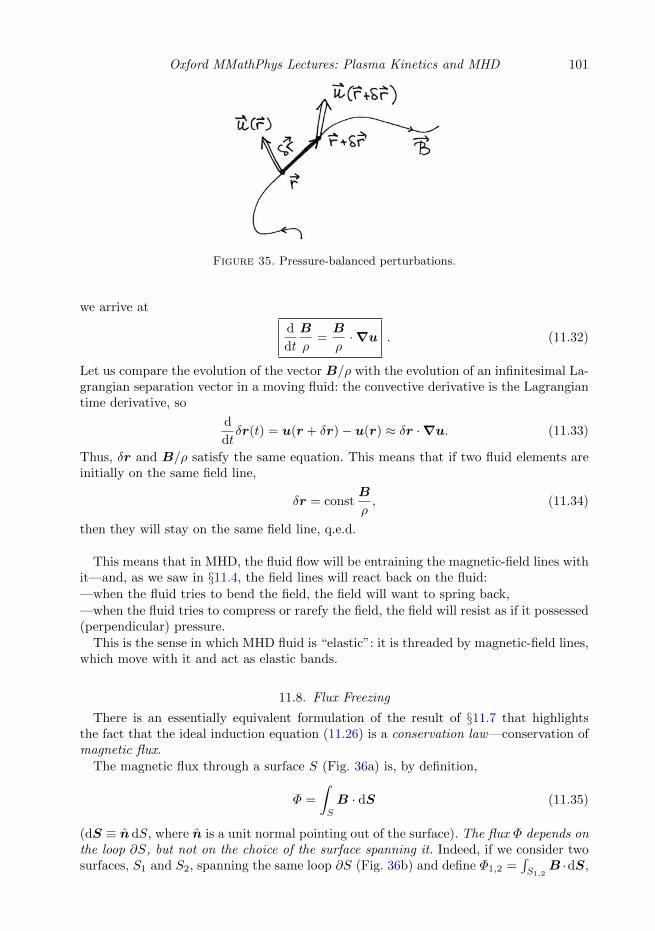
Oxford MMathPhys Lectures: Plasma Kinetics and MHD 101
Figure 35. Pressure-balanced perturbations.
we arrive at
d
dt
B
ρ=B
ρ·∇u . (11.32)
Let us compare the evolution of the vector B/ρ with the evolution of an infinitesimal La-grangian separation vector in a moving fluid: the convective derivative is the Lagrangiantime derivative, so
d
dtδr(t) = u(r + δr)− u(r) ≈ δr ·∇u. (11.33)
Thus, δr and B/ρ satisfy the same equation. This means that if two fluid elements areinitially on the same field line,
δr = constB
ρ, (11.34)
then they will stay on the same field line, q.e.d.
This means that in MHD, the fluid flow will be entraining the magnetic-field lines withit—and, as we saw in §11.4, the field lines will react back on the fluid:—when the fluid tries to bend the field, the field will want to spring back,—when the fluid tries to compress or rarefy the field, the field will resist as if it possessed(perpendicular) pressure.
This is the sense in which MHD fluid is “elastic”: it is threaded by magnetic-field lines,which move with it and act as elastic bands.
11.8. Flux Freezing
There is an essentially equivalent formulation of the result of §11.7 that highlightsthe fact that the ideal induction equation (11.26) is a conservation law—conservation ofmagnetic flux.
The magnetic flux through a surface S (Fig. 36a) is, by definition,
Φ =
∫S
B · dS (11.35)
(dS ≡ ndS, where n is a unit normal pointing out of the surface). The flux Φ depends onthe loop ∂S, but not on the choice of the surface spanning it. Indeed, if we consider twosurfaces, S1 and S2, spanning the same loop ∂S (Fig. 36b) and define Φ1,2 =
∫S1,2
B ·dS,

102 A. A. Schekochihin
(a) (b)
Figure 36. Magnetic flux through a loop ∂S (a) is independent of the surface spanning theloop (b).
Figure 37. A loop moving with the fluid.
then the flux out of the volume V enclosed by S1 ∪ S2 = ∂V is
Φ2 − Φ1 =
∫∂V
B · dS =
∫V
d3r∇ ·B = 0, q.e.d. (11.36)
Alfven’s Theorem. Flux through any loop moving with the fluid is conserved.
Proof. Let S(t) be a surface spanning the loop at time t. If the loop moves with thefluid (Fig. 37), at the slightly later time t+ dt it is spanned (for example) by the surface
S(t+ dt) = S(t) ∪ ribbon traced by the loopas it moves over time dt.
(11.37)
Then the flux at time t is
Φ(t) =
∫S(t)
B(t) · dS (11.38)

Oxford MMathPhys Lectures: Plasma Kinetics and MHD 103
Figure 38. Flux tube.
and at the later time,
Φ(t+ dt) =
∫S(t+dt)
B(t+ dt) · dS
=
∫S(t)
B(t+ dt) · dS︸ ︷︷ ︸=
∫S(t)
B(t) · dS︸ ︷︷ ︸= Φ(t)
+ dt
∫S(t)
∂B
∂t·dS
+
∫ribbon
B(t+ dt) · dS︸︷︷︸= udt×dl︸ ︷︷ ︸
= dt
∫∂S(t)
B(t) · (u× dl)
= −dt
∫∂S(t)
(u×B) · dl
= −dt
∫S(t)
[∇× (u×B)] · dS.
(11.39)
Therefore,
dΦ
dt=Φ(t+ dt)− Φ(t)
dt=
∫S(t)
[∂B
∂t−∇× (u×B)
]︸ ︷︷ ︸
ideal inductionequation (11.26)
·dS = 0, q.e.d. (11.40)
This result means that field lines are frozen into the flow. Indeed, consider a flux tubeenclosing a field line (Fig. 38). As the tube deforms, the field line stays inside it becausefluxes through the ends and sides of the tube cannot change.
Note that Ohmic diffusion breaks flux freezing, as is obvious from (11.40) if in theintegrand one uses the induction equation (11.24) keeping the resistive term.
11.9. Amplification of Magnetic Field by Fluid Flow
An interesting physical consequence of these results is that flows of conducting fluid canamplify magnetic fields. For example, consider a flow that stretches an initial cylindricaltube of length l1 and cross section S1 into a long thin spaghetto of length l2 and crosssection S2 (Fig. 39). By conservation of flux,
B1S1 = B2S2. (11.41)
By conservation of mass,
ρ1l1S1 = ρ2l2S2. (11.42)

104 A. A. Schekochihin
Figure 39. Amplification of magnetic field by stretching.
Therefore,
B2
ρ2l2=
B1
ρ1l1⇒ B2
B1=ρ2l2ρ1l1
. (11.43)
In an incompressible fluid, ρ2 = ρ1, and the field is amplified by a factor l2/l1. In acompressible fluid, the field can also be amplified by compression.
Going back to the induction equation in the form (11.27),
∂B
∂t+ u ·∇B︸ ︷︷ ︸
advection
= B ·∇u︸ ︷︷ ︸stretching
− B∇ · u︸ ︷︷ ︸compression
, (11.44)
the three terms in it are responsible for, in order, advection of the field by the flow (i.e.,the flow carrying the field around with it), “stretching” (amplification) of the field byvelocity gradients that make fluid elements longer and, finally, compression or rareficationof the field by convergent or divergent flows (unless ∇·u = 0, as it is in an incompressiblefluid).
Hence arises the famous problem of MHD dynamo: are there fluid flows that lead tosustained amplification of the magnetic fields? The answer is yes—but the flow must be3D (the absence of dynamo action in 2D is a theorem, the simplest version of which is dueto Zeldovich 1956; see Q4). Magnetic fields of planets, stars, galaxies, etc. are all believedto owe their origin and persistence to this effect. This topic requires (and merits) a moredetailed treatment (§11.10), but for now let us flag two important aspects:• resistivity, however small, turns out to be impossible to neglect because large
gradients of B appear as the field is advected by the flow;• the amplification of the field is checked by the Lorentz force once the field is strong
enough that it can act back on the flow, viz., when their energy densities becomecomparable:
B2
8π∼ ρu2
2. (11.45)
11.10. MHD Dynamo
I will fill this in at some point. You will find a (somewhat outdated) preview in myhandwritten lecture notes available here: http://www-thphys.physics.ox.ac.uk/people/AlexanderSchekochihin/notes/leshouches07.pdf.
A very short printed review is Schekochihin & Cowley (2007, §3). Another decent one is Tobiaset al. (2012). A classic (and mostly timeless) text on the mean-field dynamo theory (amplificationof large-scale magnetic fields by small-scale turbulence) is Moffatt (1978).

Oxford MMathPhys Lectures: Plasma Kinetics and MHD 105
11.11. Conservation of Energy
Let us summarise the equations that we have derived so far, namely (11.2), (11.5) and(11.24), expressing conservation of
mass∂ρ
∂t+ ∇ · (ρu) = 0, (11.46)
momentum ρ
(∂u
∂t+ u ·∇u
)= −∇p−∇ ·Π +
(∇×B)×B4π
= −∇ ·[(p+
B2
8π
)I− BB
4π+Π
]︸ ︷︷ ︸
total stress
, (11.47)
and flux∂B
∂t= ∇× (u×B) + η∇2B. (11.48)
To complete the system, we need an equation for p, which has to come from the oneconservation law that we have not yet utilised: conservation of energy.
The total energy density is
ε =ρu2
2︸︷︷︸kinetic
+p
γ − 1︸ ︷︷ ︸internal
+E2
8π︸︷︷︸electric
+B2
8π︸︷︷︸magnetic
, (11.49)
where the electric energy can (and, for consistency with §11.3, must) be neglected becauseE2/B2 ∼ u2/c2 1. We follow the same logic as we did in §§11.1 and 11.2:
d
dt
∫V
d3r ε︸ ︷︷ ︸energy insidea volume of
fluid
= −∫∂V
(ρu2
2+
p
γ − 1
)u · dS︸ ︷︷ ︸
fluid flow carrying itskinetic and internal energy
through boundary
−∫∂V
[(p I +Π) · u] · dS︸ ︷︷ ︸work done on boundaryby pressure and viscous
stress
−∫∂V
q · dS︸ ︷︷ ︸heat flux
−∫∂V
c
4π(E ×B) · dS︸ ︷︷ ︸
Poynting flux
. (11.50)
Like the viscous stress Π, the heat flux q must be calculated kinetically (in a plasma) ortabulated (in an arbitrary complicated substance). In a gas, q = −κ∇T , but it is morecomplicated in a magnetised plasma (see, e.g., Braginskii 1965; Helander & Sigmar 2005;Parra 2018a).
Note that the magnetic energy and the work done by the Lorentz force are not includedin the first two terms on the right-hand side of (11.50) because all of that must alreadybe correctly acounted for by the Poynting flux. Indeed, since cE = −u ×B + η∇ ×B
106 A. A. Schekochihin
[this is (11.13), with η renamed as in (11.24)], we have
∫∂V
c
4π(E ×B) · dS =
∫∂V
B2
8πu · dS︸ ︷︷ ︸
magnetic energyflow
+
∫∂V
[(B2
8πI− BB
4π
)· u]· dS︸ ︷︷ ︸
work done by Maxwell stress
+
∫∂V
η(∇×B)×B
4π· dS︸ ︷︷ ︸
resistive slippage accountingfor field not being precisely
frozen into flow
. (11.51)
After application of Gauss’s theorem and shrinking of the volume V to infinitesimality,we get the differential form of (11.50):
∂
∂t
(ρu2
2+
p
γ − 1+B2
8π
)=−∇ ·
[ρu2
2u+
γ
γ − 1pu+Π · u+ q
+B2I−BB
4π· u+ η
(∇×B)×B4π
]. (11.52)
It remains to separate the evolution equation for p by using the fact that we know theequations for ρ, u and B and so can deduce the rates of change of the kinetic andmagnetic energies.
11.11.1. Kinetic Energy
Using (11.46) and (11.47),
∂
∂t
ρu2
2=u2
2
∂ρ
∂t+ ρu · ∂u
∂t
= −u2
2∇ · (ρu)− ρu ·∇u2
2− u ·
∇ ·
[(p+
B2
8π
)I− BB
4π+Π
]= −∇ ·
[ρu2
2u +pu +
(B2
8πI− BB
4π
)· u +Π · u
]
+ p∇ · u︸ ︷︷ ︸compressional
work
+
(B2
8πI− BB
4π
): ∇u︸ ︷︷ ︸
energy exchangewith magnetic field
+ Π : ∇u︸ ︷︷ ︸viscous
dissipation
. (11.53)
The flux terms (energy flows and work by stresses on boundaries) that have been crossedout cancel with corresponding terms in (11.52) once (11.53) is subtracted from it.

Oxford MMathPhys Lectures: Plasma Kinetics and MHD 107
11.11.2. Magnetic Energy
Using the induction equation (11.48),
∂
∂t
B2
8π=B
4π·[−u ·∇B +B ·∇u−B∇ · u+ η∇2B
]= −∇ ·
[B2
8πu +
η
(∇×B)×B4π
]−(B2
8πI− BB
4π
): ∇u︸ ︷︷ ︸
energy exchangewith velocity field
− η|∇×B|2
4π︸ ︷︷ ︸Ohmic
dissipation
.
(11.54)
Again, the crossed out flux terms will cancel with corresponding terms in (11.52). Themetamorphosis of the resistive term into a flux term and an Ohmic dissipation term is apiece of vector algebra best checked by expanding the divergence of the flux term. Finally,the u-to-B energy exchange term (penultimate on the right-hand side) correspondsprecisely to the B-to-u exchange term in (11.53) and cancels with it if we add (11.53)and (11.54).
11.11.3. Thermal Energy
Subtracting (11.53) and (11.54) from (11.52), consummating the promised cancella-tions, and mopping up the remaining ∇ · (pu) and p∇ · u terms, we end up with thedesired evolution equation for the thermal (internal) energy:
d
dt
p
γ − 1︸ ︷︷ ︸advection of
internalenergy
= −∇ · q︸ ︷︷ ︸heat flux
− γ
γ − 1p∇ · u︸ ︷︷ ︸
compressionalheating
− Π : ∇u︸ ︷︷ ︸viscousheating
+ η|∇×B|2
4π︸ ︷︷ ︸Ohmicheating
. (11.55)
A further rearrangement and the use of the continuity equation (11.46) to express ∇·u =−d ln ρ/dt turn (11.55) into
d
dtln
p
ργ=γ − 1
p
(−∇ · q −Π : ∇u+ η
|∇×B|2
4π
). (11.56)
This form of the thermal-energy equation has very clear physical content: the left-handside represents advection of the entropy of the MHD fluid by the flow—each fluid elementbehaves adiabatically, except for the sundry non-adiabatic effects on the right-hand side.The latter are the heat flux in/out of the fluid element and the dissipative (viscousand resistive) heating, leading to entropy production. Note that the form of the viscousstress Π ensures that the viscous heating is always positive [see, e.g., (11.6)]. In theseLectures, we will, for the most part, focus on ideal MHD and so use the adiabatic versionof (11.56), with the right-hand side set to zero.

108 A. A. Schekochihin
Let us reiterate the equations of ideal MHD, now complete:
∂ρ
∂t+ ∇ · (ρu) = 0, (11.57)
ρ
(∂u
∂t+ u ·∇u
)= −∇p+
(∇×B)×B4π
, (11.58)
∂B
∂t= ∇× (u×B) , (11.59)(
∂
∂t+ u ·∇
)p
ργ= 0. (11.60)
In what follows, we shall study various solutions and symptotic regimes of these rathernice equations.
11.12. Virial Theorem
Are there self-confined states? Coming soon. . .
11.13. Lagrangian MHD
There is a mathematically attractive Lagrangian formulation of MHD, on which there is anexcellent classic paper by Newcomb (1962). Read it while this section remains unwritten.
This formalism, besides shedding some conceptual light, turns out to give us some usefulanalytical tools, e.g., for the treatment of explosive MHD instabilities (Pfirsch & Sudan 1993;Cowley & Artun 1997).
12. MHD in a Straight Magnetic Field
Equations (11.57–11.60) have a very simple static, uniform equilibrium solution:
ρ0 = const, p0 = const, u0 = 0, B0 = B0z = const. (12.1)
We will turn to more nontrivial equilibria in due course, but first we shall study this onecarefully—because it is very generic in the sense that many other, more complicated,equilibria locally look just like this.
12.1. MHD Waves
If you have an equilibrium solution of any set of equations, your first reflex ought tobe to perturb it and see what happens: the system might support waves, instabilities,possibly interesting nonlinear behaviour of small perturbations (e.g., §§7–10).
So we now seek solutions to the MHD equations (11.57–11.60) in the form
ρ = ρ0 + δρ, p = p0 + δp, u =∂ξ
∂t, B = B0z + δB, (12.2)
where we have introduced the fluid displacement field ξ.56 To start with, we consider all
56Thinking in terms of displacements makes sense in MHD but not so much in (homogeneous)hydrodynamics because in the latter case, just displacing a fluid element produces no backreaction, whereas in MHD, because magnetic fields are frozen into the fluid and are elastic,displacing fluid elements causes magnetic restoring forces to switch on. In other words, an(ideal) MHD fluid “remembers” the state from which it has been displaced, whereas neutral(Newtonian) fluids only “know” about velocities at which they flow.

Oxford MMathPhys Lectures: Plasma Kinetics and MHD 109
(a) Perpendicular perturbations, (b) Parallel perturbations,δb = δB⊥/B0 δB‖ = δB
Figure 40. Magnetic perturbations.
perturbations to be infinitesimal and so linearise the MHD equations (11.57–11.60) asfollows. (
∂
∂t+ u ·∇
)ρ = −ρ∇ · u ⇒ ∂δρ
∂t= −ρ0∇ ·
∂ξ
∂t
⇒ δρ
ρ0= −∇ · ξ , (12.3)(
∂
∂t+ u ·∇
)p
ργ= 0 ⇒ ∂
∂t
δp
p0= γ
∂
∂t
δρ
ρ0
⇒ δp
p0= −γ∇ · ξ , (12.4)(
∂
∂t+ u ·∇
)B = B ·∇u−B∇ · u ⇒ ∂δB
∂t= B0∇‖
∂ξ
∂t− zB0∇ ·
∂ξ
∂t
⇒ δB
B0= ∇‖ξ − z∇ · ξ = ∇‖ξ⊥ − z∇⊥ · ξ⊥
⇒ δB⊥B0
= ∇‖ξ⊥ ,δB‖
B0= −∇⊥ · ξ⊥ ,
(12.5)
where ‖ and ⊥ denote projections onto the direction (z) of B0 and onto the plane (x, y)perpendicular to it, respectively. Equations (12.5) tell us that parallel displacementsproduce no perturbation of the magnetic field—obviously not, because the magneticfield is carried with the fluid flow and nothing will happen if you displace a straightuniform field parallel to itself.
The physics of magnetic-field perturbations becomes clearer if we observe that
δB
B0=δ(Bb)
B0= δb+ z
δB
B0. (12.6)
The perturbed field-direction vector δb must be perpendicular to z (otherwise the fielddirection is unperturbed; formally this is shown by perturbing the equation b2 = 1).Therefore, the perpendicular and parallel perturbations of the magnetic field are theperturbations of its direction and strength, respectively (Fig. 40):
δB⊥B0
= δb,δB‖
B0=δB
B0. (12.7)

110 A. A. Schekochihin
Figure 41. Coordinate system for the treatment of MHD waves.
Finally, linearising (11.58) gives us
ρ
(∂u
∂t+ u ·∇u
)︸ ︷︷ ︸
= ρ0∂2ξ
∂t2
= −∇p︸ ︷︷ ︸= −∇δp
= γp0∇∇ · ξ,from (12.4)
−∇B2
8π︸ ︷︷ ︸= −B
20
4π∇ δB
B0
+B ·∇B
4π︸ ︷︷ ︸=B2
0
4π∇‖(δb+ z
δB
B0
).
︸ ︷︷ ︸=B2
0
4π
(−∇⊥
δB
B0+∇‖δb
)=
B20
4π
(∇⊥∇⊥ · ξ⊥ +∇2
‖ξ⊥),
from (12.7) and (12.5)
(12.8)
Assembling all this, we get
∂2ξ
∂t2= c2s∇∇ · ξ + v2
A
(∇⊥∇⊥ · ξ⊥ +∇2
‖ξ⊥), (12.9)
where two special velocities have emerged:
cs =
√γp0
ρ0, vA =
B0√4πρ0
, (12.10)
the sound speed and the Alfven speed, respectively. The former is familiar from fluiddynamics, while the latter is another speed, arising in MHD, at which perturbations cantravel. We shall see momentarily how this happens.
Let us seek wave-like solutions of (12.9), ξ ∝ exp(−iωt+ik ·r). For such perturbations,
ω2ξ = c2skk · ξ + v2A
(k⊥k⊥ · ξ⊥ + k2
‖ξ⊥). (12.11)
Without loss of generality, let k = (k⊥, 0, k‖) (i.e., by definition, x is the direction of k⊥;see Fig. 41). Then (12.11) becomes
ω2ξx = c2sk⊥(k⊥ξx + k‖ξ‖) + v2Ak
2ξx, (12.12)
ω2ξy = v2Ak
2‖ξy, (12.13)
ω2ξ‖ = c2sk‖(k⊥ξx + k‖ξ‖). (12.14)

Oxford MMathPhys Lectures: Plasma Kinetics and MHD 111
Figure 42. Hannes Olof Gosta Alfven (1908-1995), Swedish electrical engineer and plasmaphysicist. He was the father of MHD, distrusted religion, computers and Big Bang theory, andgot a Nobel Prize “for fundamental work and discoveries in magnetohydrodynamics with fruitfulapplications in different parts of plasma physics” (1970). In this picture, he is receiving it fromKing Gustaf VI Adolf of Sweden.
(a) (b) k⊥ 6= 0
Figure 43. Alfven waves.
The perturbations of the rest of the fields are
δρ
ρ0= −ik · ξ = −i(k⊥ξx + k‖ξ‖), (12.15)
δp
p0= γ
δρ
ρ0, (12.16)
δb = ik‖ξ⊥ = ik‖
ξxξy0
, (12.17)
δB
B0= −ik⊥ξx. (12.18)
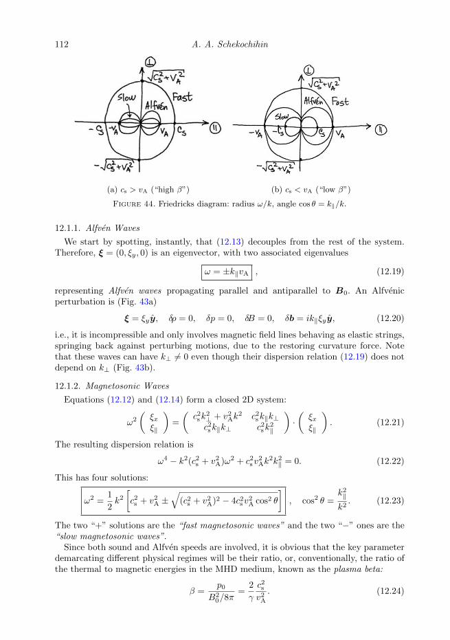
112 A. A. Schekochihin
(a) cs > vA (“high β”) (b) cs < vA (“low β”)
Figure 44. Friedricks diagram: radius ω/k, angle cos θ = k‖/k.
12.1.1. Alfven Waves
We start by spotting, instantly, that (12.13) decouples from the rest of the system.Therefore, ξ = (0, ξy, 0) is an eigenvector, with two associated eigenvalues
ω = ±k‖vA , (12.19)
representing Alfven waves propagating parallel and antiparallel to B0. An Alfvenicperturbation is (Fig. 43a)
ξ = ξyy, δρ = 0, δp = 0, δB = 0, δb = ik‖ξyy, (12.20)
i.e., it is incompressible and only involves magnetic field lines behaving as elastic strings,springing back against perturbing motions, due to the restoring curvature force. Notethat these waves can have k⊥ 6= 0 even though their dispersion relation (12.19) does notdepend on k⊥ (Fig. 43b).
12.1.2. Magnetosonic Waves
Equations (12.12) and (12.14) form a closed 2D system:
ω2
(ξxξ‖
)=
(c2sk
2⊥ + v2
Ak2 c2sk‖k⊥
c2sk‖k⊥ c2sk2‖
)·(ξxξ‖
). (12.21)
The resulting dispersion relation is
ω4 − k2(c2s + v2A)ω2 + c2sv
2Ak
2k2‖ = 0. (12.22)
This has four solutions:
ω2 =1
2k2
[c2s + v2
A ±√
(c2s + v2A)2 − 4c2sv
2A cos2 θ
], cos2 θ =
k2‖
k2. (12.23)
The two “+” solutions are the “fast magnetosonic waves” and the two “−” ones are the“slow magnetosonic waves”.
Since both sound and Alfven speeds are involved, it is obvious that the key parameterdemarcating different physical regimes will be their ratio, or, conventionally, the ratio ofthe thermal to magnetic energies in the MHD medium, known as the plasma beta:
β =p0
B20/8π
=2
γ
c2sv2
A
. (12.24)
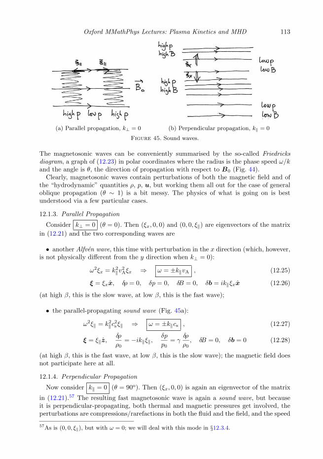
Oxford MMathPhys Lectures: Plasma Kinetics and MHD 113
(a) Parallel propagation, k⊥ = 0 (b) Perpendicular propagation, k‖ = 0
Figure 45. Sound waves.
The magnetosonic waves can be conveniently summarised by the so-called Friedricksdiagram, a graph of (12.23) in polar coordinates where the radius is the phase speed ω/kand the angle is θ, the direction of propagation with respect to B0 (Fig. 44).
Clearly, magnetosonic waves contain perturbations of both the magnetic field and ofthe “hydrodynamic” quantities ρ, p, u, but working them all out for the case of generaloblique propagation (θ ∼ 1) is a bit messy. The physics of what is going on is bestunderstood via a few particular cases.
12.1.3. Parallel Propagation
Consider k⊥ = 0 (θ = 0). Then (ξx, 0, 0) and (0, 0, ξ‖) are eigenvectors of the matrix
in (12.21) and the two corresponding waves are
• another Alfven wave, this time with perturbation in the x direction (which, however,is not physically different from the y direction when k⊥ = 0):
ω2ξx = k2‖v
2Aξx ⇒ ω = ±k‖vA , (12.25)
ξ = ξxx, δρ = 0, δp = 0, δB = 0, δb = ik‖ξxx (12.26)
(at high β, this is the slow wave, at low β, this is the fast wave);
• the parallel-propagating sound wave (Fig. 45a):
ω2ξ‖ = k2‖c
2s ξ‖ ⇒ ω = ±k‖cs , (12.27)
ξ = ξ‖z,δρ
ρ0= −ik‖ξ‖,
δp
p0= γ
δρ
ρ0, δB = 0, δb = 0 (12.28)
(at high β, this is the fast wave, at low β, this is the slow wave); the magnetic field doesnot participate here at all.
12.1.4. Perpendicular Propagation
Now consider k‖ = 0 (θ = 90o). Then (ξx, 0, 0) is again an eigenvector of the matrix
in (12.21).57 The resulting fast magnetosonic wave is again a sound wave, but becauseit is perpendicular-propagating, both thermal and magnetic pressures get involved, theperturbations are compressions/rarefactions in both the fluid and the field, and the speed
57As is (0, 0, ξ‖), but with ω = 0; we will deal with this mode in §12.3.4.
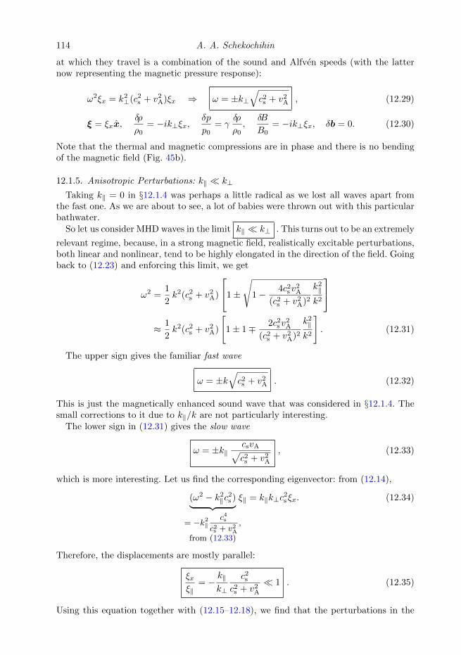
114 A. A. Schekochihin
at which they travel is a combination of the sound and Alfven speeds (with the latternow representing the magnetic pressure response):
ω2ξx = k2⊥(c2s + v2
A)ξx ⇒ ω = ±k⊥√c2s + v2
A , (12.29)
ξ = ξxx,δρ
ρ0= −ik⊥ξx,
δp
p0= γ
δρ
ρ0,
δB
B0= −ik⊥ξx, δb = 0. (12.30)
Note that the thermal and magnetic compressions are in phase and there is no bendingof the magnetic field (Fig. 45b).
12.1.5. Anisotropic Perturbations: k‖ k⊥
Taking k‖ = 0 in §12.1.4 was perhaps a little radical as we lost all waves apart fromthe fast one. As we are about to see, a lot of babies were thrown out with this particularbathwater.
So let us consider MHD waves in the limit k‖ k⊥ . This turns out to be an extremely
relevant regime, because, in a strong magnetic field, realistically excitable perturbations,both linear and nonlinear, tend to be highly elongated in the direction of the field. Goingback to (12.23) and enforcing this limit, we get
ω2 =1
2k2(c2s + v2
A)
1±
√1−
4c2sv2A
(c2s + v2A)2
k2‖
k2
≈ 1
2k2(c2s + v2
A)
[1± 1∓ 2c2sv
2A
(c2s + v2A)2
k2‖
k2
]. (12.31)
The upper sign gives the familiar fast wave
ω = ±k√c2s + v2
A . (12.32)
This is just the magnetically enhanced sound wave that was considered in §12.1.4. Thesmall corrections to it due to k‖/k are not particularly interesting.
The lower sign in (12.31) gives the slow wave
ω = ±k‖csvA√c2s + v2
A
, (12.33)
which is more interesting. Let us find the corresponding eigenvector: from (12.14),
(ω2 − k2‖c
2s )︸ ︷︷ ︸
= −k2‖c4s
c2s + v2A,
from (12.33)
ξ‖ = k‖k⊥c2s ξx. (12.34)
Therefore, the displacements are mostly parallel:
ξxξ‖
= −k‖
k⊥
c2sc2s + v2
A
1 . (12.35)
Using this equation together with (12.15–12.18), we find that the perturbations in the

Oxford MMathPhys Lectures: Plasma Kinetics and MHD 115
Figure 46. Slow wave in the anistropic limit k‖ k⊥: pressure balanced, ξx ξ‖.
remaining fields are
δρ
ρ0= −i(k⊥ξx + k‖ξ‖) = −i v2
A
c2s + v2A
k‖ξ‖, (12.36)
δp
p0= γ
δρ
ρ0, (12.37)
δb = ik‖ξxx = −ik‖
k⊥
c2sc2s + v2
A
k‖ξ‖x→ 0, (12.38)
δB
B0= −ik⊥ξx = i
c2sc2s + v2
A
k‖ξ‖. (12.39)
Thus, to lowest order in k‖/k⊥, this wave involves no bending of the magnetic field,but has a pressure/density perturbation and a magnetic-field-strength perturbation—thelatter in counter-phase to the former (Fig. 46). To be precise, the slow-wave perturbationsare pressure balanced:
δ
(p+
B2
8π
)= p0
δp
p0+B2
0
4π
δB
B0= ρ0
(c2sδρ
ρ0+ v2
A
δB
B0
)= 0. (12.40)
The same is, of course, already obvious from the momentum equation (12.8), where, inthe limit k‖ k⊥ and ω kcs (“incompressible” perturbations; see §12.2), the dominantbalance is
∇⊥(p+
B2
8π
)= 0. (12.41)
Finally, the Alfven waves in the limit of anisotropic propagation are just the sameas ever (§12.1.1)—they are unaffected by k⊥, while being perfectly capable of havingperpendicular variation (Fig. 43b).
12.1.6. High-β Limit: cs vA
Another limit in which high-frequency acoustic response (fast waves) and low-frequency, pressure-balanced Alfvenic response (slow and Alfven waves) are separatedis β 1 ⇔ cs vA.58 In this limit, the approxmate expression (12.31) for themagnetosonic frequencies is still valid, but because vA/cs, rather than k‖/k, is small.
58This limit is astrophysically very interesting because magnetic fields locally produced byplasma motions in various astrophysical environments (e.g., interstellar and intergalactic media)
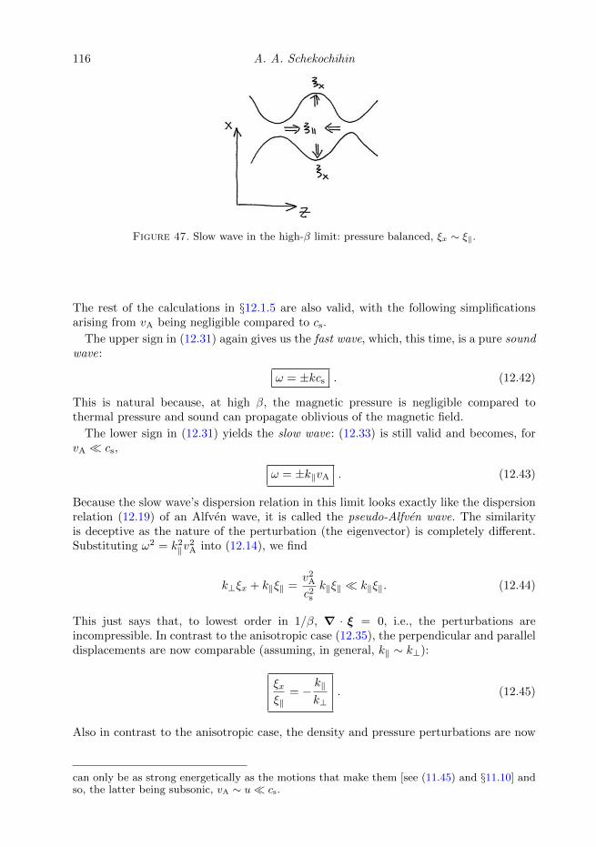
116 A. A. Schekochihin
Figure 47. Slow wave in the high-β limit: pressure balanced, ξx ∼ ξ‖.
The rest of the calculations in §12.1.5 are also valid, with the following simplificationsarising from vA being negligible compared to cs.
The upper sign in (12.31) again gives us the fast wave, which, this time, is a pure soundwave:
ω = ±kcs . (12.42)
This is natural because, at high β, the magnetic pressure is negligible compared tothermal pressure and sound can propagate oblivious of the magnetic field.
The lower sign in (12.31) yields the slow wave: (12.33) is still valid and becomes, forvA cs,
ω = ±k‖vA . (12.43)
Because the slow wave’s dispersion relation in this limit looks exactly like the dispersionrelation (12.19) of an Alfven wave, it is called the pseudo-Alfven wave. The similarityis deceptive as the nature of the perturbation (the eigenvector) is completely different.Substituting ω2 = k2
‖v2A into (12.14), we find
k⊥ξx + k‖ξ‖ =v2
A
c2sk‖ξ‖ k‖ξ‖. (12.44)
This just says that, to lowest order in 1/β, ∇ · ξ = 0, i.e., the perturbations areincompressible. In contrast to the anisotropic case (12.35), the perpendicular and paralleldisplacements are now comparable (assuming, in general, k‖ ∼ k⊥):
ξxξ‖
= −k‖
k⊥. (12.45)
Also in contrast to the anisotropic case, the density and pressure perturbations are now
can only be as strong energetically as the motions that make them [see (11.45) and §11.10] andso, the latter being subsonic, vA ∼ u cs.
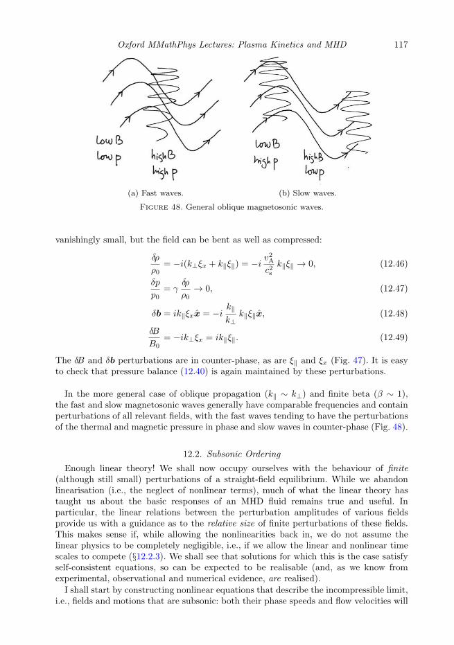
Oxford MMathPhys Lectures: Plasma Kinetics and MHD 117
(a) Fast waves. (b) Slow waves.
Figure 48. General oblique magnetosonic waves.
vanishingly small, but the field can be bent as well as compressed:
δρ
ρ0= −i(k⊥ξx + k‖ξ‖) = −i v
2A
c2sk‖ξ‖ → 0, (12.46)
δp
p0= γ
δρ
ρ0→ 0, (12.47)
δb = ik‖ξxx = −ik‖
k⊥k‖ξ‖x, (12.48)
δB
B0= −ik⊥ξx = ik‖ξ‖. (12.49)
The δB and δb perturbations are in counter-phase, as are ξ‖ and ξx (Fig. 47). It is easyto check that pressure balance (12.40) is again maintained by these perturbations.
In the more general case of oblique propagation (k‖ ∼ k⊥) and finite beta (β ∼ 1),the fast and slow magnetosonic waves generally have comparable frequencies and containperturbations of all relevant fields, with the fast waves tending to have the perturbationsof the thermal and magnetic pressure in phase and slow waves in counter-phase (Fig. 48).
12.2. Subsonic Ordering
Enough linear theory! We shall now occupy ourselves with the behaviour of finite(although still small) perturbations of a straight-field equilibrium. While we abandonlinearisation (i.e., the neglect of nonlinear terms), much of what the linear theory hastaught us about the basic responses of an MHD fluid remains true and useful. Inparticular, the linear relations between the perturbation amplitudes of various fieldsprovide us with a guidance as to the relative size of finite perturbations of these fields.This makes sense if, while allowing the nonlinearities back in, we do not assume thelinear physics to be completely negligible, i.e., if we allow the linear and nonlinear timescales to compete (§12.2.3). We shall see that solutions for which this is the case satisfyself-consistent equations, so can be expected to be realisable (and, as we know fromexperimental, observational and numerical evidence, are realised).
I shall start by constructing nonlinear equations that describe the incompressible limit,i.e., fields and motions that are subsonic: both their phase speeds and flow velocities will
118 A. A. Schekochihin
be assumed small compared to the speed of sound:
ω/k√c2s + v2
A
1, Ma ≡ u√c2s + v2
A
1. (12.50)
In this limit, we expect all fast-wave-like perturbations to disappear (in a similar wayto the sound waves disappearing in the incompressible Navier–Stokes hydrodynamics)and for the MHD dynamics to contain only Alfvenic and slow-wave-like perturbations.We saw in §§12.1.5 and 12.1.6 that, linearly, fast and slow waves are well separatedeither in the limit of k‖/k⊥ 1 or in the limit of β 1. Indeed, comparing the Alfvenfrequency (12.19) and slow-wave frequency (12.33) to the sound (fast-wave) frequency(12.32), we get
ωAlfven
ωfast∼
k‖vA
k√c2s + v2
A
∼k‖
k
1√1 + β
,ωslow
ωfast∼
k‖csvA
k(c2s + v2A)∼k‖
k
√β
1 + β, (12.51)
both of which are small in either of the two limits, satisfying the first of the conditions(12.50).
The second condition (12.50) involves the “magnetic Mach number” Ma (generalisedto compare the flow velocity to the speed of sound in a magnetised fluid), which measuresthe size of the perturbations themselves—in the linear theory, this was arbitrarily small,but now we will need to relate it to our other small parameter(s), k‖/k or 1/β. Thismeans that we would like to construct an asymptotic ordering in which there will besome prescription as to how small, or otherwise, various (relative) perturbations andsmall parameters are—not by themselves, i.e., compared to 1, but compared to eachother (compared to 1, the small parameters can all formally be taken to be as small aswe desire).
The general strategy for ordering perturbations with respect to each other will be touse the linear relations obtained in the two incompressible limits (k‖/k 1 or β 1).If we do not specifically expect one perturbation to be larger or smaller than another onsome physical grounds (like the properties of the linear response), we must order themthe same; this does not stop us later from constructing subsidiary expansions in whichthey might be different. For example, MHD equations themselves were an expansiona number of small parameters, in particular u/c [see (11.14)]. However, at the time ofderiving them, we did not want to rule out sonic or supersonic motions and so, effectively,we ordered Ma ∼ 1, k‖/k ∼ 1 and β ∼ 1, as far as the u/c expansion was concerned, i.e.,Ma, k‖/k, 1/β u/c. Now we are constructing a subsidiary expansion in these otherparameters, keeping in mind that they are allowed to be small but not as small as thesmall parameter already used in the derivation of the MHD equations.59
12.2.1. Ordering of Alfvenic Perturbations
Since the Alfvenic perturbations decouple completely from the rest (§12.1.1), lineartheory does not give us a way to relate uy to u‖, so we will exercise the no-prejudiceprinciple stated above and assume
uy ∼ u‖, (12.52)
59In principle, you should always feel a little paranoid about the question of whether such“nested” asymptotic expansions commute, i.e., whether it matters in which order they are done.They usually do commute, but you ought to check if you want to be sure. Another formallyjustified mathematical worry is whether asymptotic solutions of exact equations are the same asexact solutions of asymptotic equations. This will lead you into the world of proofs of existenceand uniqueness—where I wish you an enjoyable stay.
Oxford MMathPhys Lectures: Plasma Kinetics and MHD 119
i.e., the Mach numbers for the Alfvenic and slow-wave-like motions are comparable. Wecan, however, relate uy to δb, via the curvature-force response (12.20):
|δb| ∼ k‖ξy ∼k‖uy
ω∼ uyvA∼ Ma
√1 + β. (12.53)
12.2.2. Ordering of Slow-Wave-Like Perturbations
For slow-wave-like perturbations, in either the anisotropic or the high-β limit, from(12.14) and (12.33),
∇ · u ∼ ω(k⊥ξx + k‖ξ‖) ∼ω2
k‖c2sωξ‖ ∼
v2A
c2s + v2A
k‖u‖ ∼k‖u‖
1 + β. (12.54)
Thus, the divergence of the flow velocity is small (the dynamics are incompressible) inall three of our (potentially) small parameters:
∇ · uk√c2s + v2
A
∼k‖
k
1
1 + βMa. (12.55)
From this, we can immediately obtain an ordering for the density and pressure pertur-bations: using (12.3), (12.4), (12.33) and (12.54) [cf. (12.36) and (12.46)],
δρ
ρ0∼ δp
p0∼∇ · ξ ∼ ∇ · u
ω∼ Ma√
β. (12.56)
The magnetic-field-strength (magnetic-pressure) perturbation is, using (12.39) and(12.33) [cf. (12.49)],
δB
B0∼ k⊥ξx ∼
c2sc2s + v2
A
k‖u‖
ω∼√βMa, (12.57)
or, perhaps more straightforwardly, from pressure balance (12.40) and using (12.56),
δB
B0= −β
2
δp
p0∼√βMa. (12.58)
Finally, in a similar fashion, using (12.17) and (12.57) [cf. (12.38) and (12.48)], we find
|δb| ∼ k‖ξx ∼k‖
k⊥
√βMa (12.59)
for slow-wave-like perturbations. Note that in all interesting limits this is superceded bythe Alfvenic ordering (12.53).
12.2.3. Ordering of Time Scales
Let us recall that our motivation for using linear relations between perturbations todetermine their relative sizes in a nonlinear regime was that linear response will loseits exclusive sway but remain non-negligible. In formal terms, this means that we mustorder the linear and nonlinear time scales to be comparable.60 The nonlinearities in MHDequations are advective, i.e., they are of the form u ·∇(stuff) and similar, so the rateof nonlinear interaction is ∼ ku (in the case of anisotropic perturbations, ∼ k⊥u⊥).Ordering this to be comparable to the frequencies of the Alfven and slow waves [see
60In the context of MHD turbulence theory, this principle, applied at each scale, is known asthe critical balance (see §12.4).
120 A. A. Schekochihin
(12.51)] gives us
ωAlfven ∼ ku ⇒ Ma ∼k‖
k
1√1 + β
, (12.60)
ωslow ∼ ku ⇒ Ma ∼k‖
k
√β
1 + β. (12.61)
Note that the first of these relations supersedes the second in all interesting limits.
12.2.4. Summary of Subsonic Ordering
Thus, the ordering of the time scales determines the size of the perturbationsvia (12.60). Using this restriction on Ma, we may summarise our subsonic ordering asfollows61
Ma ≡ u√c2s + v2
A
∼ |δb|√1 + β
∼ 1√β
δB
B∼√βδρ
ρ0∼√βδp
p0∼k‖
k
1√1 + β
1 (12.62)
and ω ∼ ku. The ordering can be achieved either in the limit of k‖/k 1 or 1/β 1,or both. Note that if one of these parameters is small, the other can be order unity oreven large (as long as it is not larger than the inverse of the small one).
The case of anisotropic perturbations and arbitrary β applies in a broad range ofplasmas, from magnetically confined fusion ones (tokamaks, stellarators) to space (e.g.,the solar corona or the solar wind). We shall consider the implications of this orderingin §12.3.
The case of high β applies, e.g., to high-energy galactic and extragalactic plasmas.It is the direct generalisation to MHD of incompressible Navier–Stokes hydrodynamics,i.e., in this case, all one needs to do is solve MHD equations assuming ρ = const and∇ · u = 0. We shall consider this case now.
12.2.5. Incompressible MHD Equations
Assuming β 1, our ordering becomes
u
cs∼ ω
kcs∼ 1√
β∼ Ma, |δb| ∼ δB
B0∼√βMa ∼ 1,
δρ
ρ0∼ δp
p0∼ Ma√
β∼ Ma2 .
(12.63)Thus, the density and pressure perturbations are minuscule, while magnetic perturbationsare order unity—magnetic fields are relatively easy to bend (i.e., subsonic motions cantangle the field substantially in this regime). Because of this, it will not make sense tosplit B into B0 and δB explicitly, we will treat the magnetic field as a single field, withno need for a strong mean component.
Let us examine the MHD equations (11.57–11.60) under the ordering (12.63).Since ω ∼ ku, the convective derivative d/dt = ∂/∂t + u ·∇ survives intact in all
equations, allowing the advective nonlinearity to enter.The continuity equation (11.57) simply reiterates our earlier statement that the velocity
field is divergenceless to lowest order:
∇ · u = −1
ρ
dρ
dt∼ ω δρ
ρ0∼ Ma3kcs → 0. (12.64)
61Note that it is not absolutely necessary to work out the detailed linear theory of a set ofequations in order to be able to construct such orderings: it is often enough to know roughlywhere you are going and simply balance terms representing the physics that you wish to keep(or expect to have to keep). An example of this approach is given in §12.2.8.
Oxford MMathPhys Lectures: Plasma Kinetics and MHD 121
The momentum equation (11.58) becomes(1 +δρ
ρ0
)(∂u
∂t+ u ·∇u
)= −∇
(c2sγ
δp
p0+
B2
8πρ0
)︸ ︷︷ ︸
≡ p
+B ·∇B
4πρ0. (12.65)
The density perturbation in the left-hand side is ∼ Ma2 and so negligible compared tounity. The remaining terms in this equation are all the same order (∼ Ma2kc2s ) and sothey must all be kept. The total “pressure” p is determined by enforcing ∇ · u = 0 [see(12.64)]. Namely, our equations are
∂u
∂t+ u ·∇u = −∇p+B ·∇B , (12.66)
where
∇2p = −∇∇ : (uu−BB) (12.67)
and we have rescaled the magnetic field to velocity units, B/√
4πρ0 → B.In the induction equation, best written in the form (11.27), all terms are the same
order ∼ kuB ∼ Ma kcsB except the one containing ∇ · u, which is ∼ Ma3kcsB and somust be neglected. We are left with
∂B
∂t+ u ·∇B = B ·∇u . (12.68)
Finally, the internal-energy equation (11.60), which, keeping only the lowest-orderterms, becomes (
∂
∂t+ u ·∇
)(δp
p0− γ δρ
ρ0
)= 0, (12.69)
can be used to find δρ/ρ0, once δp/p0 = γ(p − B2/2)/c2s is calculated from the solutionof (12.66–12.68). Note that δρ/ρ0 is merely a spectator quantity, not required to solve(12.66–12.68), which form a closed set.
Equations (12.66–12.68) are the equations of incompressible MHD (let us call itiMHD). Note that while they have been obtained in the limit of β 1, all β dependencehas disappeared from them—basically, they describe subsonic dynamics on top of aninfinite heat bath. This is how it should be: formally, in any good asymptotic theory,it must be possible to make the small parameter artbitrarily small without changinganything in the equations.
Exercise 12.1. Show that iMHD conserves the sum of kinetic and magnetic energies,
d
dt
∫d3r
(u2
2+B2
2
)= 0. (12.70)
Exercise 12.2. Check that you can obtain the right waves, viz., Alfven (§12.1.1) and pseudo-Alfven (§12.1.6), directly from iMHD.
12.2.6. Elsasser MHD
The iMHD equations possess a remarkable symmetry. Let us introduce Elsasser (1950)fields
Z± = u±B (12.71)

122 A. A. Schekochihin
and rewrite (12.66) and (12.68) as evolution equations for Z±: after trivial algebra,
∂Z±
∂t+Z∓ ·∇Z± = −∇p (12.72)
and, since ∇ ·Z± = 0,
∇2p = −∇∇ : Z+Z−. (12.73)
Thus, one can think of iMHD as representing the evolution of two incompressible “velocityfields” advecting each other.
Let us restore the separation of the magnetic field into its mean and perturbed parts,B = B0 + δB = vAz + δB (recall that B is in velocity units). Then
Z± = ±vAz + δZ± (12.74)
and (12.72) becomes
∂δZ±
∂t∓ vA∇‖δZ± + δZ∓ ·∇δZ± = −∇p . (12.75)
Thus, δZ± are finite, counter-propagating (at the Alfven speed vA) perturbations—andthey interact nonlinearly only with each other, not with themselves. If we let, say, δZ− =0⇔ u = δB, then δZ+ satisfies
∂δZ+
∂t− vA∇‖δZ+ = 0, (12.76)
and similarly for δZ− (propagting at −vA) if δZ+ = 0. Therefore,
δZ± = f(r ± vAtz), δZ∓ = 0, (12.77)
where f is an arbitrary function, are exact nonlinear solutions of iMHD. They are calledElsasser states. Physically, they are isolated Alfven-wave packets that propagate alongthe guide field and never interact (because they all travel at the same speed and so cannever catch up with or overtake one another). In order to have any interesting nonlineardynamics, the system must have counter-propagating Alfven-wave packets (see §12.4).
12.2.7. Cross-Helicity
Equations (12.72) manifestly support two conservation laws:
d
dt
∫d3r|Z±|2
2= 0, (12.78)
i.e., the energy of each Elsasser field is individually conserved. This can be reformulatedas conservation of the total energy,
d
dt
∫d3r
1
2
(|Z+|2
2+|Z−|2
2
)=
d
dt
∫d3r
(u2
2+B2
2
)= 0, (12.79)
and of a new quantity, known as the cross-helicity:
d
dt
∫d3r
1
2
(|Z+|2
2− |Z
−|2
2
)=
d
dt
∫d3r u ·B = 0 . (12.80)

Oxford MMathPhys Lectures: Plasma Kinetics and MHD 123
In the Elsasser formulation, the cross-helicity is a measure of energy imbalace betweenthe two Elssasser fields62—this is observed, for example, in the solar wind, where thereis significantly more energy in the Alfvenic fluctuations propagating away from the Sunthan towards it (see, e.g., Wicks et al. 2013).
Exercise 12.3. To see why we needed incompressibility to get this new conservation law, workout the time evolution equation for
∫d3r u ·B from the general (compressible) MHD equations
and hence the condition under which the cross-helicity is conserved.
12.2.8. Stratified MHD
It is quite instructive to consider a very simple example of non-uniform MHD equilibrium:the case of a stratified atmosphere. Let us introduce gravity into MHD equations, viz., themomentum equation (11.58) becomes
ρdu
dt= −∇
(p+
B2
8π
)+B ·∇B
4π− ρgz (12.81)
(uniform gravitational acceleration pointing downward, against the z direction). We wish toconsider a static equilibrium inhomogeneous in the z direction and threaded by a uniformmagnetic field (which may be zero):
ρ0 = ρ0(z), p0 = p0(z), u0 = 0, B0 = B0b0 = const, (12.82)
where b0 is at some general angle to z and p0(z) and ρ0(z) are constrained by the vertical forcebalance:
dp0dz
= −ρ0g ⇒ g = −p0ρ0
d ln p0dz
=c2sγ
1
Hp, (12.83)
where it has been opportune to define the pressure scale height Hp. We shall now seek time-dependent solutions of the MHD equations for which
ρ = ρ0(z) + δρ,δρ
ρ0 1, p = p0(z) + δp,
δp
p0 1, (12.84)
and the spatial variation of all pertubations occurs on scales that are small compared to thepressure scale height Hp or the analogously defined density scale height Hρ = −(d ln ρ0/dz)
−1
(for ordering purposes, we denote them both H):
kH 1 . (12.85)
After the equilibrium pressure balance is subtracted from (12.81), this equation becomes,under any ordering in which δρ ρ0,
ρ0du
dt= −∇
(δp+
B2
8π
)+B ·∇B
4π− δρgz . (12.86)
The last term is the buoyancy (Archimedes) force. In order for this new feature to give rise toany nontrivial new physics, it must be ordered comparable to all the other terms in the equation:using (12.83) to express g ∼ p0/ρ0H, we find
δρg ∼ kδp ⇒ δρ
ρ0∼ kH δp
p0 δp
p0, (12.87)
δρg ∼ kB2
4π⇒ δρ
ρ0∼ kH
β 1 ⇒ β kH 1. (12.88)
So we learn that the density perturbations must now be much larger than the pressure pertur-bations, but, in order for the former to remain small and for the magnetic field to be in the
62Cross-helicity can also be interpreted as a topological invariant, counting the linkages betweenflux tubes and vortex tubes analogously to what magnetic helicity does for the flux tubes alone(see §13.2).

124 A. A. Schekochihin
game, β must be high (it is in anticipation of this that we did not split B into B0 and δB,expecting them to be of the same order).
Let us now expand the internal-energy equation (11.60) in small density and pressure pertur-bations. Denoting s = p/ργ = s0(z) + δs (entropy density) and introducing the entropy scaleheight
1
Hs≡ d ln s0
dz= − 1
Hp+
γ
Hρ(12.89)
(assumed positive), we find63
d
dt
δs
s0= − uz
Hs,
δs
s0=δp
p0− γ δρ
ρ0≈ −γ δρ
ρ0. (12.90)
The last, approximate, expression follows from the smallness of pressure perturbations [see(12.87)]. This then gives us
d
dt
δρ
ρ0=
uzγHs
. (12.91)
But, on the other hand, the continuity equation (11.57) is
d
dt
δρ
ρ0= −∇ · u+
uzHρ
⇒ ∇ · u = uz
(1
Hρ− 1
γHs
)=
uzγHp
⇒ ∇ · uku
∼ 1
kH 1.
(12.92)Thus, the dynamics are incompressible again and the role of the continuity equation is to tellus that we must find δp from the momentum equation (12.86) by enforcing ∇ · u = 0 to lowestorder. The difference with iMHD (§12.2.5) is that δρ/ρ now participates in the dynamics via thebuoyancy force and must be found self-consistently from (12.91).
Finally, we rewrite our newly found simplified system of equations for a stratified, high-βatmosphere, in the following neat way:
∂u
∂t+ u ·∇u = −∇p+B ·∇B + az, (12.93)
∇2p = −∇∇ : (uu−BB) +∂a
∂z, (12.94)
∂a
∂t+ u ·∇a = −N2uz, N =
cs
γ√HsHp
, (12.95)
∂B
∂t+ u ·∇B = B ·∇u, (12.96)
where we have rescaled B/√
4πρ0 → B and denoted the Archimedes acceleration
a = − δρρ0g = − δρ
ρ0
c2sγHp
, (12.97)
a quantity also known as the buoyancy of the fluid. We shall call (12.93–12.96) the equations ofstratified MHD (SMHD).
A new frequency N , known as the Brunt–Vaisala frequency, has appeared in our equations.64
In order for all the linear and nonlinear time scales that are present in our equations to coexistlegitimately within our ordering, we must demand that the Alfven, Brunt–Vaisala and nonlineartime scales all be comparable:
kvA ∼ N ∼ ku ⇒ 1√β∼ 1
kH∼ Ma . (12.98)
This gives us a relative ordering between all the small parameters that have appeared so far,
63We are able to take equilibrium quantities in and out of spatial derivatives because kH 1and the perturbations are small.64N is real because we assumed Hs > 0 (a “stably stratified atmosphere”), otherwisethe atmosphere becomes convectively unstable—this happens when the equilibrium entropydecreases upwards (cf. §14.3, Q9 and Q5c).

Oxford MMathPhys Lectures: Plasma Kinetics and MHD 125
including the new one, 1/kH. Using (12.91) and recalling (12.87), let us summarise the orderingof the perturbations:
u
cs∼ δρ
ρ0∼ Ma,
δp
p0∼ Ma2, |δb| ∼ δB
B0∼ 1. (12.99)
The difference with the iMHD high-β ordering (12.63) is that the density perturbations havenow been promoted to dynamical relevance, thankfully without jeopardising incompressibility(i.e., still ordering out the sonic perturbations). The ordering (12.99) can be thought of as ageneralisation to MHD of the Boussinesq approximation in hydrodynamics.
Further investigations of the SMHD equations are undertaken in Q5.
12.3. Reduced MHD
We now turn to the anisotropic ordering, k‖/k 1 (while β ∼ 1, in general), for whichwe studied the linear theory in §12.1.5. Specialising to this case from our general ordering(12.62), we have
Ma ∼ u⊥cs∼u‖
cs∼ |δb| ∼ δB
B0∼ δρ
ρ0∼ δp
p0∼ ω
k⊥cs∼k‖
k⊥ 1 . (12.100)
Starting again with the continuity equation (11.57), dividing through by ρ0 andordering all terms, we get(
∂
∂t︸︷︷︸Ma
+u⊥ ·∇⊥︸ ︷︷ ︸Ma
+
u‖ · ∇‖︸ ︷︷ ︸Ma2
)δρ
ρ0︸︷︷︸Ma︸ ︷︷ ︸
Ma2
= −(
1 +δρ
ρ0︸︷︷︸Ma
)(∇⊥ · u⊥︸ ︷︷ ︸
Ma
+∇‖u‖︸ ︷︷ ︸Ma2
)︸ ︷︷ ︸
Ma
. (12.101)
Thus, to lowest order, the perpendicular velocity field is 2D-incompressible:
O(Ma) : ∇⊥ · u⊥ = 0 . (12.102)
In the next order (which we will need in §12.3.2),
O(Ma2) : (∇ · u)2 = −(∂
∂t+ u⊥ ·∇⊥
)δρ
ρ0= − d
dt
δρ
ρ0, (12.103)
where, to leading order, the convective derivative now involves only perpendicular ad-vection.
Equation (12.102) implies that u⊥ can be written in terms of a stream function:
u⊥ = z ×∇⊥Φ . (12.104)
Similarly, for the magnetic field, we have
0 = ∇ ·B = ∇⊥ · δB⊥︸ ︷︷ ︸Ma
+∇‖δB‖︸ ︷︷ ︸
Ma2
≈∇⊥ · δB⊥, (12.105)
so δB⊥ is also 2D-solenoidal and can be written in terms of a flux function:
δB⊥√4πρ0
= z ×∇⊥Ψ . (12.106)
Note that Ψ = −A‖/√
4πρ0, the parallel component of the vector potential.Thus, Alfvenically polarised perturbations, u⊥ and δB⊥ (see §12.1.1), can be described
by two scalar functions, Φ and Ψ . Let us work out the evolution equations for them.
126 A. A. Schekochihin
12.3.1. Alfvenic Perturbations
We start with the induction equation, again most useful in the form (11.27). Dividingthrough by B0, we have
d
dt
δB
B0= b ·∇u− b∇ · u. (12.107)
Throwing out the obviously subdominant δb contribution in the last term on the right-hand side (i.e., approximating b ≈ z in that term), then taking the perpendicular partof the remaining equation, we get
d
dt
δB⊥B0
= b ·∇u⊥. (12.108)
As we saw above, the convective derivative is with respect to the perpendicular velocityonly and, in view of the stream-function representation (12.104) of the latter, for anyfunction f , we have, to leading order,
df
dt=∂f
∂t+ u⊥ ·∇⊥f =
∂f
∂t+ z · (∇⊥Φ×∇⊥f) =
∂f
∂t+ Φ, f, (12.109)
where the “Poisson bracket” is
Φ, f =∂Φ
∂x
∂f
∂y− ∂Φ
∂y
∂f
∂x. (12.110)
Similarly, to leading order,
b ·∇f =∂f
∂z+ δb ·∇⊥f =
∂f
∂z+
1
vAz · (∇⊥Ψ ×∇⊥f) =
∂f
∂z+
1
vAΨ, f. (12.111)
Finally, using (12.109) and (12.111) in (12.108) and expressing δB⊥ in terms of Ψ [see(12.106)] and u⊥ in terms of Φ [see (12.104)], it is a straightforward exercise to show,after “uncurling” (12.108), that65
∂Ψ
∂t+ Φ, Ψ = vA
∂Φ
∂z. (12.112)
Turning now to the momentum equation (11.58), taking its perpendicular part anddividing through by ρ ≈ ρ0, we get
du⊥dt︸ ︷︷ ︸Ma2
=1
ρ0
[−∇⊥
(p+
B2
8π
)+B ·∇δB⊥
4π
]= −∇⊥
(c2sγ
δp
p0+ v2
A
δB
B0
)︸ ︷︷ ︸
Ma
+ v2Ab ·∇
δB⊥B0︸ ︷︷ ︸
Ma2
.
(12.113)To lowest order,
O(Ma) : ∇⊥(c2sγ
δp
p0+ v2
A
δB
B0
)= 0 ⇒ δp
p0= −γ v
2A
c2s
δB
B0. (12.114)
This is a statement of pressure balance, which is physically what has been expected [see(12.41)] and which will be useful in §12.3.2. In the next order, (12.113) contains theperpendicular gradient of the second-order contribution to the total pressure. To avoid
65Another easy route to this equation is to start from the induction equation in the form (11.59),let B = ∇×A, “uncurl” (11.59) and take the z component of the resulting evolution equationfor A.

Oxford MMathPhys Lectures: Plasma Kinetics and MHD 127
having to calculate it, we take the curl of (12.113) and thus obtain
O(Ma2) : ∇⊥ ×du⊥dt
= v2A∇⊥ ×
(b ·∇δB⊥
B0
). (12.115)
Finally, using again (12.104), (12.106), (12.109) and (12.111) in (12.115), some slightlytedious algebra leads us to
∂
∂t∇2⊥Φ+ Φ,∇2
⊥Φ = vA∂
∂z∇2⊥Ψ + Ψ,∇2
⊥Ψ . (12.116)
Note that ∇2⊥Φ is the vorticity of the flow u⊥ and so the above equation is the MHD
generalisation of the 2D Euler equation.To summarise the equations (12.116) and (12.112) in their most compact form, we
have
d
dt∇2⊥Φ = vAb ·∇∇2
⊥Ψ, (12.117)
dΨ
dt= vA
∂Φ
∂z, (12.118)
where the convective time derivative d/dt and the parallel spatial derivative b·∇ are givenby (12.109) and (12.111), respectively. Beautifully, these nonlinear equations describingAlfvenic perturbations have decoupled completely from everything else: we do not needto know δρ, δp, u‖ or δB in order to solve for u⊥ and δB⊥. Alfvenic dynamics are self-contained.
Equations (12.117) and (12.118) are called the Equations of Reduced MHD (RMHD).They were originally derived in the context of tokamak plasmas (Kadomtsev & Pogutse1974; Strauss 1976) and are extremely popular as a simple paradigm for MHD is a strongguide field—not just in tokamaks, but also in space.66
12.3.2. Compressive Perturbations
What about the rest of our fields—in the linear language, the slow-wave-like pertur-bations (§12.1.5)? While we do not need them to compute the Alfvenic perturbations,we might still wish to know them for their own sake.
Returning to the induction equation (12.107) and taking its z component, we get
d
dt
δB‖
B0= b ·∇u‖ −∇ · u ⇒ d
dt
(δB
B0− δρ
ρ0
)= b ·∇u‖ , (12.119)
where all terms are O(Ma2), δB‖ ≈ δB to leading order and we used (12.103) to express∇ ·u. The derivatives d/dt and b ·∇ contain the nonlinearities involving Φ and Ψ , whichwe already know from (12.117) and (12.118).
To find an equation for u‖, we take the z component of the momentum equation(11.58):
du‖
dt︸︷︷︸Ma2
=1
ρ0
[−
∂
∂z
(p+
B2
8π
)︸ ︷︷ ︸
Ma3
+B ·∇δB‖
4π︸ ︷︷ ︸Ma2
]⇒
du‖
dt= v2
Ab ·∇δB
B0. (12.120)
66In the latter context, they are used most prominently as a description of Alfvenic turbulenceat small scales (see §12.4), for which the RMHD equations can be shown to be the correctdescription even if the plasma is collisionless and in general requires kinetic treatment(Schekochihin et al. 2009; Kunz et al. 2015, 2018).

128 A. A. Schekochihin
The parallel pressure gradient is O(Ma3) because there is pressure balance (12.114) tolowest order.
Finally, let us bring in the energy equation (11.60), as yet unused. To leading order,it is
d
dt
δs
s0=
d
dt
(δp
p0− γ δρ
ρ0
)= 0 ⇒ d
dt
(δρ
ρ0+v2
A
c2s
δB
B0
)= 0 , (12.121)
where, to obtain the final version of the equation, we substituted (12.114) for δp/p0.Equations (12.119–12.121) are a complete set of equations for δB, u‖ and δρ, given Φ
and Ψ . These equations are linear in the Lagrangian frame associated with the Alfvenicperturbations, provided the parallel distances are measured along perturbed field lines.Physically, they tell us that slow waves propagate along perturbed field lines and arepassively (i.e., without acting back) advected by the perpendicular Alfvenic flows.
Exercise 12.4. Check that the linear relationships between various perturbations in a slowwave derived in §12.1.5 are manifest in (12.119–12.121).
In what follows, when we refer to RMHD, we will mean all five equations (12.117–12.118) and (12.119–12.121).
Exercise 12.5. Show that RMHD equations possess the following exact symmetry: ∀ ε and a,one can simultaneously scale all perturbation amplitudes by ε, perpendicular distances by a,parallel distances and times by a/ε. This means that parallel and perpendicular distances inRMHD are effectively measured in different units. It also means that the small parameter Main RMHD can be made arbitrarily small, without any change in the form of the equations, soRMHD is a bona fide asymptotic theory (see remark at the end of §12.2.5).
12.3.3. Elsasser Fields and the Energetics of RMHD
The Elsasser approach (§12.2.6) can be adapted to the RMHD system. DefiningElsasser potentials
ζ± = Φ± Ψ ⇔ δZ±⊥ = u⊥ ±δB⊥√4πρ0
= z ×∇⊥ζ±, (12.122)
it is a straighforward exercise to show that the “vorticities” of the the two Elsasser fields,
ω± = z · (∇⊥ × δZ±⊥) = ∇2⊥ζ± (12.123)
(fluid vorticities ± electric currents), satisfy the following evolution equation
∂ω±
∂t∓ vA
∂ω±
∂z+ ζ∓, ω± = ∂jζ±, ∂jζ∓ , (12.124)
where summation over the repeated index j is implied. The main corrolary of thisequation is the same as in §12.2.6, although here it applies to perpendicular perturbationsonly: only counter-propagting Alfvenic perturbations can interact and any finite-amplitudeperturbation composed of just one Elsasser field is a nonlinear solution.
Some light is perhaps shed on the nature of the interaction between Elasser fields if we noticethat the left-hand side of (12.124) tells us that the Elsasser vorticity ω± is propagated alongthe mean field at the speed vA and advected across the field by the Elsasser field δZ∓⊥. Theright-hand side of (12.124) is a kind of vortex-stretching term, implying a tendency for vorticesand current layers to be produced in the (x, y) plane. There is a preference for current layers,as it turns out. The term in the right-hand side of (12.124) has opposite signs for the twoElsasser fields. Therefore, arguably, nonlinear dynamics favour ω+ω− < 0, i.e., |∇2
⊥Ψ |2 > |∇2⊥Φ|2
Oxford MMathPhys Lectures: Plasma Kinetics and MHD 129
(larger currents than vorticities). This is, indeed, what is seen in numerical simulations of MHDturbulence (see Zhdankin et al. 2016 and §12.4).
The energies of the two Elsasser fields are individually conserved (cf. §12.2.7),
d
dt
∫d3r |∇⊥ζ±|2 =
d
dt
∫d3r |δZ±⊥|
2 = 0, (12.125)
i.e., when the two fields do interact, they scatter each other nonlinearly, but do notexchange energy.
There is an Elsasser-like formulation for the slow waves as well:67
δZ±‖ = u‖ ±δB√4πρ0
√1 +
v2A
c2s. (12.126)
Then, from (12.119–12.121), one gets, after more algebra,
∂δZ±‖
∂t∓ csvA√
c2s + v2A
∂δZ±‖
∂z=
− 1
2
[(1∓ 1√
1 + v2A/c
2s
)ζ+, δZ±‖ +
(1± 1√
1 + v2A/c
2s
)ζ−, δZ±‖
].
(12.127)
Note the (expected) appearance of the slow-wave phase speed [cf. (12.33)] in the left-handside. Thus, slow waves interact only with Alfvenic perturbations—when vA cs, onlywith the counterpropagating ones, but at finite β, because the slow waves are slower, aco-propagating Alfvenic perturbation can catch up with a slow one, have its way with itin passing and speed on (it’s a tough world).
There is no energy exchange in these interactions: the “+” and “−” slow-wave energiesare individually conserved:
d
dt
∫d3r |δZ±‖ |
2 = 0. (12.128)
12.3.4. Entropy Mode
There are only two equations in (12.127), whereas we had three equations (12.119–12.121) for our three compressive fields δB, u‖ and δρ. The third equation, (12.121), wasin fact for the entropy perturbation:
dδs
dt= 0 ,
δs
s0= −γ
(δρ
ρ0+v2
A
c2s
δB
B0
). (12.129)
We see that δs is a decoupled variable, independent from ζ± or δZ±‖ (because it is the
only one that involves δρ/ρ0). Equation (12.129) says that δs is a passive scalar field,simply carried around by the Alfvenic velocity u⊥ (via d/dt). At high β, this is just adensity perturbation.
The associated linear mode is not a wave: its dispersion relation is
ω = 0 . (12.130)
This is the (famously often forgotten) 7th MHD mode, known as the entropy mode (there
67At high β, vA cs, so we recover from (12.126) and (12.122) the Elsasser fields as defined foriMHD in (12.71).
130 A. A. Schekochihin
are 7 equations in MHD, so there must be 7 linear modes: two fast waves, two Alfvenwaves, two slow waves and one entropy mode).
Exercise 12.6. Go back to §12.1 and find where we overlooked this mode.
Since the entropy mode is decoupled, its “energy” (variance) is individually conserved:
d
dt
∫d3r |δs|2 = 0. (12.131)
Thus, in RMHD, the (nonlinear) evolution of all perturbations is constrained by 5 separateconservation laws:
∫d3r |δZ±⊥|2,
∫d3r |δZ±‖ |
2 and∫
d3r |δs|2 are all invariants.
12.3.5. Discussion
Such are the simplifications allowed by anisotropy. Besides greater mathematicalsimplicity, what is the moral of this story, physically? Let me leave you with twoobservations.
• In a strong magnetic field, linear propagation is a parallel effect, whilst nonlinearityis a perpendicular effect (advection by u⊥, adjustment of propagation direction byδB⊥). RMHD equations express the idea that linear and nonlinear physics play equallyimportant role—this becomes the fundamental guiding principle in the theory of MHDturbulence (§12.4). The idea is that complicated nonlinear dynamics that emerge in theperpendicular plane get teased out along the field because propagating waves enforce adegree of parallel spatial coherence. The distances over which this happens are determinedby equating linear and nonlinear time scales, k‖vA ∼ k⊥u⊥. Dynamics cannot stay
coherent over distances longer than ∼ k−1‖ determined by this balance because of
causality: points separated by longer parallel distances cannot exchange informationquickly enough to catch up with perpendicular nonlinearities acting locally at each ofthese points. This principle is called critical balance.
• Restricting the size of perturbations to be small made the RMHD system, in acertain sense, “less nonlinear” than the full MHD (or than iMHD, where δB/B0 ∼ 1 wasallowed). This led to the system’s dynamics being constrained by more invariants: theMHD energy invariant got split into 5 individually conserved quadratic quantities.
Exercise 12.7. You might find it an interesting excercise to think about properties of theRMHD system in 2D, in the light of the two observations above. How many invariants are there?In what kind of physical circumstances can we use 2D RMHD without necessarily expectingparallel coherence of the system to break down by the causality argument?
12.4. MHD Turbulence
RMHD is a good starting point for developing the theory of MHD turbulence—a phenomenonobserved with great precision in the solar wind and believed ubiquitous in the Universe. I amwriting a tutorial review of this topic—a reasonably advanced draft can be found here: http://www-thphys.physics.ox.ac.uk/research/plasma/JPP/papers17/schekochihin2a.pdf.
13. MHD Relaxation
So far, we have only considered MHD in a straight field against the background ofconstant density and pressure (except in §12.2.8, where this was generalised slightly). Asany more complicated (static) equilibrium will locally look like this, what we have done
Oxford MMathPhys Lectures: Plasma Kinetics and MHD 131
has considerable universal significance. Now we shall occupy ourselves with a somewhatless universal (i.e., dependent on the circumstances of a particular problem) and more“large-scale” (compared to the dynamics of wavy perturbations) question: what kind of(static) equilibrium states are there and into which of those states will an MHD fluidnormally relax?
13.1. Static MHD Equilibria
Let us go back to the MHD equations (11.57–11.60) and seek static equilibria, i.e., setu = 0 and ∂/∂t = 0. The remaining equations are
−∇p+j ×Bc
= 0, j =c
4π∇×B, ∇ ·B = 0 (13.1)
(the force balance, Ampere’s law and the solenoidality-of-B constraint). These are 7equations for 7 unknowns (p, B, j), so a complete set. Density is irrelevant becausenothing moves and so inertia does not matter.
The force-balance equation has two immediate general consequences:
B ·∇p = 0, (13.2)
so magnetic surfaces are surfaces of constant pressure, and
j ·∇p = 0, (13.3)
so currents flow along those surfaces.Equation (13.2) implies that if magnetic field lines are stochastic and fill the volume
of the system, then p = const across the system and so the force balance becomes
j ×B = 0. (13.4)
Such equilibria are called force-free and turn out to be very interesting, as we shalldiscover soon (from §13.1.2 onwards).
13.1.1. MHD Equilibria in Cylindrical Geometry
As the simplest example of an inhomogeneous equilibrium, let us consider the case ofcylindrical and axial symmetry:
∂
∂θ= 0,
∂
∂z= 0. (13.5)
Solenoidality of the magnetic field then rules out it having a radial component:
∇ ·B =1
r
∂
∂rrBr = 0 ⇒ rBr = const ⇒ Br = 0. (13.6)
Ampere’s law tells us that currents do not flow radially either:
j =c
4π∇×B ⇒
jr = 0,
jθ = − c
4π
∂Bz∂r
,
jz =c
4π
1
r
∂
∂rrBθ.
(13.7)

132 A. A. Schekochihin
(a) (b) Plasma is confined.
Figure 49. z pinch.
Finally, the radial pressure balance gives us
∂p
∂r=
(j ×B)rc
=jθBz − jzBθ
c=
1
4π
(−Bz
∂Bz∂r− Bθ
r
∂
∂rrBθ
)= − ∂
∂r
B2z
8π− B2
θ
4πr− ∂
∂r
B2θ
8π⇒ ∂
∂r
(p+
B2
8π
)= − B
2θ
4πr. (13.8)
This simply says that the total pressure gradient is balanced by the tension force. Ageneral equilibrium for which this is satisfied is called a screw pinch.
One simple particular case of this is the z pinch (Fig. 49a). This is achieved by lettinga current flow along the z axis, giving rise to an azimuthal field:
jθ = 0, jz =c
4π
1
r
∂
∂rrBθ ⇒ Bθ =
4π
c
1
r
∫ r
0
dr′r′jz(r′), Bz = 0. (13.9)
Equation (13.8) becomes
∂p
∂r= −1
cjzBθ . (13.10)
The “pinch” comes from magnetic loops and is due to the curvature force: the loopswant to contract inwards, the pressure gradient opposes this and so plasma is confined(Fig. 49b). This configuration will, however, prove to be very badly unstable (§14.4)—which does not stop it from being a popular laboratory set up for short-term confinementexperiments (see, e.g., review by Haines 2011).
Another simple particular case is the θ pinch (Fig. 50a). This is achieved by imposinga straight but radially non-uniform magnetic field in the z direction and, therefore,azimuthal currents:
Bθ = 0, jz = 0, jθ = − c
4π
∂Bz∂r
. (13.11)
Equation (13.8) is then just a pressure balance, pure and simple:
∂
∂r
(p+
B2z
8π
)= 0 . (13.12)
In this configuration, we can confine the plasma (Fig. 50c) or the magnetic flux (Fig. 50d).The latter is what happens, for example, in flux tubes that link sunspots (Fig. 50b). Theθ pinch is a stable configuration (Q10).
The more general case of a screw pinch (13.8) is a superposition of z and θ pinches, withboth magnetic fields and currents wrapping themselves around cylindrical flux surfaces.

Oxford MMathPhys Lectures: Plasma Kinetics and MHD 133
(a) (b) Coronal loop.
(c) Plasma is confined. (d) Magnetic field is confined.
Figure 50. θ pinch.
The next step in complexity is to assume axial, but not cylindrical symmetry (∂/∂θ = 0,∂/∂z 6= 0). This is explored in Q8.
For a much more thorough treatment of MHD equilibria, the classic textbook is Freidberg (2014).
13.1.2. Force-Free Equilibria
Another interesting and elegant class of equilibria arises if we consider situations inwhich ∇p is negligible and can be completely omitted from the force balance. This canhappen in two possible sets of circumstances:
—pressure is the same across the system, e.g., because the field lines are stochastic[a previously mentioned consequence of (13.2)];
—β = p/(B2/8π) 1, so thermal energy is negligible compared to magnetic energy andso p is irrelevant.
A good example of the latter situation is the solar corona, where β ∼ 1−10−6 (assumingn ∼ 109 cm−3, T ∼ 102 eV and B ∼ 1 − 103 G, the lower value applying in thephotosphere, the upper one in the coronal loops; see Fig. 50b)
In such situations, the equilibrium is purely magnetic, i.e., the magnetic field is “force-free,” which implies that the current must be parallel to the magnetic field:
j ×B = 0 ⇒ j ‖ B ⇒ 4π
cj = ∇×B = α(r)B, (13.13)
where α(r) is an arbitrary scalar function. Taking the divergence of the last equationtells us that
B ·∇α = 0, (13.14)
so the function α(r) is constant on magnetic surfaces. If B is chaotic and volume-filling,then α = const across the system.
The case of α = const is called the linear force-free field. In this case, taking the curl

134 A. A. Schekochihin
of (13.13) and then iterating it once gives us
−∇2B = α∇×B = α2B ⇒(∇2 + α2
)B = 0 , (13.15)
so the magnetic field satisfies a Helmholtz equation (to solve which, one must, of course,specify some boundary conditions).
Thus, there is, potentially, a large zoo of MHD equilibria. Some of them are stable,some are not, and, therefore, some are more interesting and/or more relevant than others.How does one tell? A good question to ask is as follows. Suppose we set up some initialconfiguration of magnetic field (by, say, switching on some current-carrying coils, drivingcurrents inside plasma, etc.)—to what (stable) equilibrium will this system eventuallyrelax?
In general, any initially arranged magnetic configuration will exert forces on theplasma, these will drive flows, which in turn will move the magnetic fields around;eventually, everything will settle into some static equilibrium. We expect that, normally,some amount of the energy contained in the initial field will be lost in such a relaxationprocess because the flows will be dissipating, the fields diffusing and/or reconnecting,etc.—the losses occur due to the resistive and viscous terms in the non-ideal MHDequations derived in §11. Thus, one expects that the final relaxed static state will be aminimum-energy state and so we must be able to find it by minimising magnetic energy:∫
d3rB2
8π→ min . (13.16)
Clearly, if the relaxation occured without any constraints, the solution would just beB = 0. In fact, there are constraints. These constraints are topological: if you thinkof magnetic field lines as a tangled mess, you will realise that, while you can changethis tangle by moving field lines around, you cannot easily undo linkages, knots, etc.—anything that, to be undone, would require the field lines to have “ends”. This intuitioncan be turned into a quantitative theory once we discover that the induction equation(11.59) has an invariant that involves the magnetic field only and is, in a certain sense,“better conserved” than energy.
13.2. Helicity
Magnetic helicity in a volume V is defined as
H =
∫V
d3rA ·B , (13.17)
where A is the vector potential, ∇×A = B.
13.2.1. Helicity Is Well Defined
This is not obvious because A is not unique: a gauge transformation
A→ A+ ∇χ, (13.18)
with χ an arbitrary scalar function, leaves B unchanged and so does not affect physics.Under this transformation, helicity stays invariant:
H → H +
∫V
d3rB ·∇χ = H +
∫∂V
dS ·B χ = H, (13.19)
provided B at the boundary is parallel to the boundary, i.e., provided the volume Vencloses the field (nothing sticks out).

Oxford MMathPhys Lectures: Plasma Kinetics and MHD 135
13.2.2. Helicity Is Conserved
Let us go back to the induction equation (11.23) (in which we retain resistivity to keeptrack of non-ideal effects, i.e., of the breaking of flux conservation):
∂B
∂t= ∇× (u×B − η∇×B) . (13.20)
“Uncurling” this equation, we get
∂A
∂t= u×B − η∇×B + ∇χ. (13.21)
Using (13.20) and (13.21), we have
∂
∂tA ·B = B · (u×B − η∇×B + ∇χ) +A · [∇× (u×B − η∇×B)]
= −ηB · (∇×B) + ∇ · (Bχ)
−∇ · [A× (u×B − η∇×B)] + (u×B − η∇×B) · (∇×A)︸ ︷︷ ︸
= B
= ∇ · [Bχ− uA ·B +BA · u+ ηA× (∇×B)]− 2ηB · (∇×B). (13.22)
Integrating this and using Gauss’s theorem, we get
∂
∂t
∫V
d3rA ·B =
∫∂V
dS · [Bχ− uA ·B +BA · u+ ηA× (∇×B)]
− 2η
∫V
d3rB · (∇×B). (13.23)
The surface integral vanishes provided both u and B are parallel to the boundary (nofields stick out and no flows cross). The resistive term in the surface integral can alsobe ignored either by arranging V appropriately or simply by taking it large enough soB → 0 on ∂V , or, indeed, by taking η → +0. Thus,
dH
dt= −2η
∫d3rB · (∇×B) , (13.24)
magnetic helicity is conserved in ideal MHD.68
Furthermore, it turns out that even in resistive MHD, helicity is “better conserved”than energy, in the following sense. As we saw in §11.11.2, the magnetic energy evolvesaccording to
d
dt
∫d3r
B2
8π=
(energy exchange terms
and fluxes
)− 2η
∫d3r |∇×B|2. (13.25)
The first term on the right-hand side contains various fluxes and energy exchanges withthe velocity field [see (11.54)], all of which eventually decay as the system relaxes (flowsdecay by viscosity). The second term represents Ohmic heating. If η is small but theOhmic heating is finite, it is finite because magnetic field develops fine-scale gradients:∇ ∼ η−1/2, so
− 2η
∫d3r |∇×B|2 → const as η → +0. (13.26)
68The resistive term in the right-hand side of (13.24) is ∝∫
d3rB · j, a quantity known as thecurrent helicity.

136 A. A. Schekochihin
Figure 51. Linked flux tubes.
But then the right-hand side of (13.24) is
− 2η
∫d3rB · (∇×B) = O(η1/2)→ 0 as η → +0. (13.27)
Thus, as an initial magnetic configuration relaxes, while its energy can change quickly(on dynamical times), its helicity changes only very slowly in the limit of small η. Theconstancy of H (as η → +0) provides us with the constraint subject to which the energywill need to be minimised.
Before we use this idea, let us discuss what the conservation of helicity means physically,or, rather, topologically.
13.2.3. Helicity Is a Topological Invariant
Consider two linked flux tubes, T1 and T2 (Fig. 51). The helicity of T1 is the productof the fluxes through T1 and T2:
H1 =
∫T1
d3rA ·B =
∫T1
dl︸︷︷︸bdl
· dS︸︷︷︸bdS
A ·B︸ ︷︷ ︸A · bB
=
∫T1
A · bdl Bb · bdS =
∫T1
A · dlB · dS = Φ1
∫T1
A · dl︸ ︷︷ ︸=∫S1B · dS
= Φthrough hole in T1
= Φ1Φ2. (13.28)
By the same token, in general, in a system of many linked tubes, the helicity of tube i is
Hi = ΦiΦthrough hole in tube i = Φi∑j
ΦjNij , (13.29)
where Nij is the number of times tube j passes through the hole in tube i. The totalhelicity of the this entire assemblage of flux tubes is then
H =∑ij
ΦiΦjNij . (13.30)
Thus, H is the number of linkages of the flux tubes weighted by the field strength inthem. It is in this sense that helicity is a topological invariant.
Note that the cross-helicity∫
d3r u · B (§12.2.7) can similarly be interpreted as counting the
linkages between flux tubes (B) and vortex tubes (ω = ∇×u). The current helicity∫
d3rB · j

Oxford MMathPhys Lectures: Plasma Kinetics and MHD 137
Figure 52. John Bryan Taylor (born 1929), one of the founding fathers of modern plasmaphysics, author of the Taylor relaxation (§13.3), Taylor constraint (in dynamo theory),Chirikov–Taylor map (in chaos theory), the ballooning theory (in tokamak MHD), and manyother clever things, including the design of the UK’s first hydrogen bomb (1957). This picturewas taken in 2012 at the Wolfgang Pauli Institute in Vienna.
[appearing in the right-hand side of (13.24)] counts the number of linkages between currentloops. The latter is not an MHD invariant though.
13.3. J. B. Taylor Relaxation
Let us now work out the equilibrium to which an MHD system will relax by minimisingmagnetic energy subject to constant helicity:
δ
∫V
d3r(B2 − αA ·B
)= 0, (13.31)
where α is the Lagrange multiplier introduced to enforce the constant-helicity constraint.Let us work out the two terms:
δ
∫V
d3rB2 = 2
∫V
d3rB · δB = 2
∫V
d3rB · (∇× δA)
= 2
∫V
d3r [−∇ · (B × δA) + (∇×B) · δA]
= −2
∫∂V
dS · (B × δA) + 2
∫V
d3r (∇×B) · δA, (13.32)
δH = δ
∫V
d3rA ·B =
∫V
d3r (B · δA+A · δB) =
∫V
d3r [B · δA+A · (∇× δA)]
=
∫V
d3[B · δA−∇ · (A× δA) + (∇×A)︸ ︷︷ ︸
= B
·δA]
= −∫∂V
dS · (A× δA) + 2
∫V
d3rB · δA. (13.33)
Now, since
∂δB
∂t= ∇× (u×B) = ∇×
(∂ξ
∂t×B
)(13.34)

138 A. A. Schekochihin
for small displacements, we have δA = ξ ×B, whence
B × δA = B2ξ −B · ξB, (13.35)
A× δA = A ·B ξ −A · ξB. (13.36)
Therefore, the surface terms in (13.32) and (13.33) vanish if B and ξ are parallel tothe boundary ∂V , i.e., if the volume V encloses both B and the plasma—there are nodisplacements through the boundary.
This leaves us with
δ
∫V
d3r(B2 − αA ·B
)= 2
∫V
d3r (∇×B − αB) · δA = 0, (13.37)
which instantly implies that B is a linear force-free field:
∇×B = αB ⇒ ∇2B = −α2B . (13.38)
Thus, our system will relax to a linear force-free state determined by (13.38) andsystem-specific boundary conditions. Here α = α(H) depends on the (fixed by initialconditions) value of H via the equation
H(α) =
∫d3rA ·B =
1
α
∫d3rB2, (13.39)
where B is the solution of (13.38) (since ∇×B = αB = α∇×A, we have B = αA+∇χand the χ term vanishes under volume integration).
Thus, the prescription for finding force-free equilibria is
—solve (13.38), get B = B(α), parametrically dependent on α,—calculate H(α) according to (13.39),—set H(α) = H0, where H0 is the initial value of helicity, hence calculate α = α(H0)
and complete the solution by using this α in B = B(α).
Note that it is possible for this procedure to return multiple solutions. In that case, thesolution with the smallest energy must be the right one (if a system relaxed to a localminimum, one can always imagine it being knocked out of it by some perturbation andfalling to a lower energy).
Exercise 13.1. Force-free fields in 2D. Show that for MHD confined to the 2D plane (x, y),the quantity
∫d2rA2
z is conserved. Work out the 2D version of J. B. Taylor relaxation and showthat the resulting equilibrium field is a linear force-free field.
13.4. Relaxed Force-Free State of a Cylindrical Pinch
Let us illustrate how the procedure derived in §13.3 works by considering again thecase of cylindrical and axial symmetry [see (13.5)]. The z component of (13.38) gives usthe following equation for Bz(r):
B′′z +1
rB′z + α2Bz = 0. (13.40)
This is a Bessel equation, whose solution, subject to Bz(0) = B0 and Bz(∞) = 0, is
Bz(r) = B0J0(αr) . (13.41)

Oxford MMathPhys Lectures: Plasma Kinetics and MHD 139
Figure 53. Relaxed cylindrical pinch.
We can now calculate the azimuthal field as follows
αBθ = (∇×B)θ = −B′z ⇒ Bθ(r) = B0J1(αr) . (13.42)
This gives us an interesting twisted field (Fig. 53), able to maintain itself in equilibriumwithout help from pressure gradients.
Finally, we calculate its helicity according to (13.39): assuming that the length of thecylinder is L, its radius R and so its volume V = πR2L, we have
H =1
α
∫d3rB2 =
2πLB20
α
∫ R
0
drr[J2
0 (αr) + J21 (αr)
]=B2
0V
α2
[J2
0 (αR) + 2J21 (αR) + J2
2 (αR)− 2
αRJ1(αR)J2(αR)
]. (13.43)
If we solve this for α = α(H), our solution is complete.
Exercise 13.2. Work out what happens in the general case of ∂/∂θ 6= 0 and ∂/∂z 6= 0 andwhether the simple symmetric solution obtained above is the correct relaxed, minimum-energystate (not always, it turns out). This is not a trivial exercise. The solution is in Taylor & Newton(2015, §9), where you will also find much more on the subject of J. B. Taylor relaxation, relaxedstates and much besides—all from the original source.
There are other useful variational principles—other in the sense that the constraints that areimposed are different from helicity conservation. The need for them arises when one considersmagnetic equilibria in domains that do not completely enclose the field lines, i.e., when dS·B 6= 0at the boundary. One example of such a variational principle, also yielding a force-free field(although not necessarily a linear one), is given in Q1(e). A specific example of such a fieldarises in Q8(f).
13.5. Parker’s Problem and Topological MHD
Coming soon. . . On topology in MHD, a very mathematically minded student might enjoythe book by Arnold & Khesin (1999).

140 A. A. Schekochihin
14. MHD Stability and Instabilities
We now wish to take a more general view of the MHD stability problem: given somestatic69 equilibrium (some ρ0, p0, B0 and u0 = 0), will this equilibrium be stable tosmall perturbations of it, i.e., will these perturbations grow or decay?
There are two ways to answer this question:
1) Carry out the normal-mode analysis, i.e., linearise the MHD equations around thegiven equilibrium, just as we did when we studied MHD waves in §12.1, and see if anyof the frequencies (solutions of the dispersion relation) turn out to be complex, withpositive imaginary parts (growth rates). This approach has the advantage of being directand also of yielding specific information about rates of growth or decay, the character ofthe growing and decaying modes, etc. However, for spatially complicated equilibria, thisis often quite difficult to do and one might be willing to settle for less: just being ableto prove that some configuration is stable or that certain types of perturbations mightgrow. Hence the the second approach:
2) Check whether, for a given equilibrium, all possible perturbations will lead to theenergy of the system increasing. If so, then the equilibrium is stable—this is called theenergy principle and we shall prove it shortly. If, on the other hand, certain perturbationslead to the energy decreasing, that equilibrium is unstable. The advantage of this secondapproach is that we do not need to solve the (linearised) MHD equations in order topronounce on stability, just to examine the properties of the perturbed energy functional.
It should be already quite clear how to do the normal-mode analysis, at least concep-tually, so I shall focus on the second approach.
14.1. Energy Principle
Recall what the total energy in MHD is (§11.11)
E =
∫d3r
(ρu2
2+B2
8π+
p
γ − 1
)≡∫
d3rρu2
2+W. (14.1)
As we saw in §12.1, all perturbations of an MHD system away from equilibrium can beexpressed in terms of small displacements ξ—we will work this out shortly for a generalequilibrium, but for now, let us accept that this will be true.70 As u = ∂ξ/∂t by definitionof ξ, we have
E =
∫d3r
1
2ρ0
∣∣∣∣∂ξ∂t∣∣∣∣2 +W0 + δW1[ξ] + δW2[ξ, ξ] + . . . , (14.2)
where we have kept terms up to second order in ξ and so W0 is the equilibrium part ofW (i.e., its value for ξ = 0), δW1[ξ] is linear in ξ, δW2[ξ, ξ] is bilinear (quadratic), etc.Energy must be conserved to all orders, so
dEdt
=
∫d3r ρ0
∂2ξ
∂t2︸ ︷︷ ︸≡ F [ξ]
·∂ξ∂t
+ δW1
[∂ξ
∂t
]+ δW2
[∂ξ
∂t, ξ
]+ δW2
[ξ,∂ξ
∂t
]+ · · · = 0. (14.3)
69A treatment of the more general case of a dynamic equilibrium, u0 6= 0, can be found in theexcellent textbook by Davidson (2016).70In fact, also the fully nonlinear dynamics can be completely expressed in terms of displacementsif the MHD equations are written in Lagrangian coordinates (see §11.13).

Oxford MMathPhys Lectures: Plasma Kinetics and MHD 141
This must be true at all times, including at t = 0, when ξ and ∂ξ/∂t can be chosen inde-pendently (MHD equations are second-order in time if written in terms of displacements).Therefore, for arbitrary functions ξ and η,∫
d3r η · F [ξ] + δW1[η] + δW2[η, ξ] + δW2[ξ,η] + · · · = 0. (14.4)
In the first order, this tells us that
δW1[η] = 0, (14.5)
which is good to know because it means that δW1 disappears from (14.2) (there are nofirst-order energy perturbations). In the second order, we get∫
d3r η · F [ξ] = −δW2[η, ξ]− δW2[ξ,η]. (14.6)
Let η = ξ. Then (14.6) implies
δW2[ξ, ξ] = −1
2
∫d3r ξ · F [ξ] . (14.7)
This is the part of the perturbed energy in (14.2) that can be both positive and negative.The Energy Principle is
δW2[ξ, ξ] > 0 for any ξ ⇔ equilibrium is stable (14.8)
(Bernstein et al. 1958). Before we are in a position to prove this, we must do somepreparatory work.
14.1.1. Properties of the Force Operator F [ξ]
Since the right-hand side of (14.6) is symmetric with respect to swapping ξ ↔ η, somust be the left-hand side: ∫
d3r η · F [ξ] =
∫d3r ξ · F [η]. (14.9)
Therefore, operator F [ξ] is self-adjoint. Since, by definition,
F [ξ] = ρ0∂2ξ
∂t2, (14.10)
the eigenmodes of this operator satisfy
ξ(t, r) = ξn(r)e−iωnt ⇒ F [ξn] = −ρ0ω2nξn. (14.11)
As always for self-adjoint operators, we can prove a number of useful statements.
1) The eigenvalues ω2n are real.
Proof. If (14.11) holds, so must
F [ξ∗n] = −ρ0(ω2n)∗ξ∗n, (14.12)
provided F has no complex coefficients (we shall confirm this explicitly in §14.2.1). Takingthe full scalar products (including integarting over space) of (14.11) with ξ∗n and of (14.12)

142 A. A. Schekochihin
(a) Instability. (b) “Overstability” (does not happen in MHD).
Figure 54. MHD instabilities.
with ξn and subtracting one from the other, we get
−[ω2n − (ω2
n)∗] ∫
d3r ρ0|ξn|2︸ ︷︷ ︸> 0
=
∫d3r ξ∗n · F [ξn]−
∫d3r ξn · F [ξ∗n] = 0
⇒ ω2n = (ω2
n)∗ , q.e.d. (14.13)
This result implies that, if any MHD equilibrium is unstable, at least one of the eigenvaluesmust be ω2
n < 0 and, since it is guaranteed to be real, any MHD instability will give riseto purely growing modes (Fig. 54a), rather than growing oscillations (also known as“overstabilities”; see Fig. 54b).
2) The eigenmodes ξn are orthogonal.
Proof. Taking the full scalar products of (14.11) with ξm (assuming m 6= n andnon-degeneracy of ω2
m,n), and of the analogous equation
F [ξm] = −ρ0ω2mξm (14.14)
with ξn and subtracting them, we get71
− (ω2n − ω2
m)︸ ︷︷ ︸6= 0
∫d3r ρ0ξn · ξm =
∫d3r ξm · F [ξn]−
∫d3r ξn · F [ξm] = 0
⇒∫
d3r ρ0ξn · ξm = δnm
∫d3r ρ0|ξn|2 , q.e.d.
(14.15)
14.1.2. Proof of the Energy Principle (14.8)
Let us assume completeness of the set of eigenmodes ξn (not, in fact, an indispensableassumption, but we shall not worry about this nuance here; see Kulsrud 2005, §7.2). Thenany displacement at any given time t can be decomposed as
ξ(t, r) =∑n
an(t)ξn(r). (14.16)
71Note that in view of (14.13), we can take ξn to be real.

Oxford MMathPhys Lectures: Plasma Kinetics and MHD 143
The energy perturbation (14.7) is
δW2[ξ, ξ] = −1
2
∫d3r ξ · F [ξ] = −1
2
∑nm
anam
∫d3r ξn · F [ξm]
=1
2
∑nm
anamω2m
∫d3r ρ0ξn · ξm︸ ︷︷ ︸use (14.15)
=1
2
∑n
a2nω
2n
∫d3r ρ0|ξn|2. (14.17)
By the same token,
K[ξ, ξ] ≡ 1
2
∫d3r ρ0|ξ|2 =
1
2
∑n
a2n
∫d3r ρ0|ξn|2. (14.18)
Then, if we arrange ω21 6 ω2
2 6 . . . , the smallest eigenvalue is
ω21 = min
ξ
δW2[ξ, ξ]
K[ξ, ξ]. (14.19)
Therefore,• condition (14.8) is sufficient for stability because, if δW2[ξ, ξ] > 0 for all possible ξ,
then the smallest eigenvalue ω21 > 0, and so all eigenvalues are positive, ω2
n > ω21 > 0;
• condition (14.8) is necessary for stability because, if the equilibrium is stable, thenall eigenvalues are positive, ω2
n > 0, whence δW2[ξ, ξ] > 0 in view of (14.17), q.e.d.
14.2. Explicit Calculation of δW2
Now that we know that we need the sign of δW2 to ascertain stability (or otherwise),it is worth working out δW2 as an explicit function of ξ. It is a second-order quantity, but(14.7) tells us that all we need to calculate is F [ξ] to first order in ξ, i.e., we just needto linearise the MHD equations around an arbitrary static equilibrium. The procedure isthe same as in §12.1, but without assuming ρ0, p0 and B0 to be spatially homogeneous.
14.2.1. Linearised MHD Equations
Thus, generalising somewhat the procedure adopted in (12.3–12.5), we have
∂ρ
∂t+ ∇ · (ρu) = 0 ⇒ ∂δρ
∂t= −∇ ·
(ρ0∂ξ
∂t
)⇒ δρ = −∇ · (ρ0ξ) , (14.20)(
∂
∂t+ u ·∇
)p = −γp∇ · u ⇒ ∂δp
∂t= −∂ξ
∂t·∇p0 − γp0∇ ·
∂ξ
∂t
⇒ δp = −ξ ·∇p0 − γp0∇ · ξ , (14.21)
∂B
∂t= ∇× (u×B) ⇒ ∂δB
∂t= ∇×
(∂ξ
∂t×B0
)⇒ δB = ∇× (ξ ×B0) . (14.22)
Note that again δρ, δp and δB are all expressed as linear operators on ξ—and so δW =δ∫
d3r[B2/8π + p/(γ − 1)
]must also be some operator involving ξ and its gradients
but not ∂ξ/∂t (as we assumed in §14.1).Finally, we deal with the momentum equation (to which we add gravity as this will

144 A. A. Schekochihin
give some interesting instabilities):
ρ
(∂u
∂t+ u ·∇u
)= −∇p+
(∇×B)×B4π
+ ρg. (14.23)
This gives us
F [ξ] = ρ0∂2ξ
∂t2= −∇δp+
(∇×B0)× δB4π
+(∇× δB)×B0
4π+ δρ g
= ∇ (ξ ·∇p0 + γp0∇ · ξ)− g∇ · (ρ0ξ) +j0 × δB
c+
(∇× δB)×B0
4π, (14.24)
where j0 = c(∇×B0)/4π, we have used (14.20) and (14.21) for δρ and δp, respectively,and δB is given by (14.22).
14.2.2. Energy Perturbation
Now we can use (14.24) in (14.7) to calculate explicitly
δW2 =1
2
∫d3r
[−ξ ·∇ (ξ ·∇p0 + γp0∇ · ξ)︸ ︷︷ ︸= (ξ ·∇p0)∇·ξ+γp0(∇·ξ)2
after integration by parts
+ (g · ξ)∇ · (ρ0ξ)
− (j0 × δB) · ξc︸ ︷︷ ︸
=j0 · (ξ × δB)
c
− (∇× δB)×B0
4π· ξ︸ ︷︷ ︸
=(∇× δB) · (ξ ×B0)
4πby parts
=(δB ×∇) · (ξ ×B0)
4π
=δB · [∇× (ξ ×B0)]
4π
=|δB|2
4π, using (14.22)
]. (14.25)
Thus, we have arrived at a standard textbook (e.g., Kulsrud 2005) expression forthe energy perturbation (this expression is non-unique because one can do variousintegrations by parts):
δW2 =1
2
∫d3r
[(ξ ·∇p0)∇ · ξ + γp0(∇ · ξ)2 + (g · ξ)∇ · (ρ0ξ)
+j0 · (ξ × δB)
c+|δB|2
4π
], (14.26)
where δB = ∇ × (ξ ×B0). Note that two of the terms inside the integral (the secondand the fifth) are positive-definite and so always stabilising. The terms that are not sign-definite and so potentially destabilising involve equilibrium gradients of pressure, densityand magnetic field (currents). It is perhaps not a surprise to learn that Nature, withits fundamental yearning for thermal equilibrium, might dislike gradients—while it is ofcourse not a rule that all such inhomogeneities render the system unstable, we will seethat they often do, usually when gradients exceed certain critical thresholds.
All we need to do now is calculate δW2 according to (14.26) for any equilibrium that

Oxford MMathPhys Lectures: Plasma Kinetics and MHD 145
interests us and see if it can be negative for any class of perturbations (or show that itis positive for all perturbations).
14.3. Interchange Instabilities
As the first and simplest example of how one does stability calculations using theEnergy Principle, we will (perhaps disappointingly) consider a purely hydrodynamicsituation: the stability of a simple hydrostatic equilibrium describing a generic stratifiedatmosphere:
ρ0 = ρ0(z) and p0 = p0(z) satisfyingdp0
dz= −ρ0g (14.27)
(gravity acts downward, against the z direction, g = −gz).
14.3.1. Formal Derivation of the Schwarzschild Criterion
With B0 = 0 and the hydrostatic equilibrium (14.27), (14.26) becomes
δW2 =1
2
∫d3r
[ξzp′0∇ · ξ + γp0(∇ · ξ)2 − gξz(ρ′0ξz + ρ0∇ · ξ)
]=
1
2
∫d3r
[2p′0ξz∇ · ξ + γp0(∇ · ξ)2 − ρ′0gξ2
z
], (14.28)
where we have used ρ0g = −p′0. We see that δW2 depends on ξz and ∇ · ξ. Let us treatthem as independent variables and minimise δW2 with respect to them (i.e., seek themost unstable possible situation):
∂
∂(∇ · ξ)
[integrandof (14.28)
]= 2p′0ξz + 2γp0(∇ · ξ) = 0 ⇒ ∇ · ξ = − p′0
γp0ξz. (14.29)
Substituting this back into (14.28), we get
δW2 =1
2
∫d3r
(− p′20γp0− ρ′0g
)ξ2z =
1
2
∫d3r
ρ0g
γ
(p′0p0− γ ρ
′0
ρ0
)︸ ︷︷ ︸
=d
dzlnp0ργ0
ξ2z . (14.30)
By the Energy Principle, the system is stable iff
δW2 > 0 ⇔ d ln s0
dz> 0 , (14.31)
where s0 = p0/ργ0 is the entropy function. The inequality (14.31) is the Schwarzschild
criterion for convective stability.72 If this criterion is broken, there will be an instability,called the interchange instability.
This calculation illustrates both the power and the weakness of the method:—on the one hand, we have obtained a stability criterion quite quickly and without
having to solve the underlying equations,—on the other hand, while we have established the condition for instability, we have
as yet absolutely no idea what is going on physically.
72We studied perturbations of a stably stratified atmosphere in §12.2.8 and Q5, where we sawthat these perturbations indeed did not grow provided the entropy scale length 1/Hs = d ln s0/dzwas positive.

146 A. A. Schekochihin
Figure 55. Interchange instability.
14.3.2. Physical Picture
We can remedy the latter problem by examining what type of displacements give riseto δW2 < 0 when the Schwarzschild criterion is broken. Recalling (14.20) and (14.21) andspecialising to the displacements given by (14.29) (as they are the ones that minimiseδW2), we get
δp
p0= −ξ ·∇p0
p0− γ∇ · ξ = −p
′0
p0ξz − γ∇ · ξ = 0, (14.32)
δρ
ρ0= − 1
ρ0∇ · (ρ0ξ) = −ρ
′0
ρ0ξz −∇ · ξ =
1
γ
(−γ ρ
′0
ρ0+p′0p0
)=
1
γ
d ln s0
dz︸ ︷︷ ︸< 0
(unstable)
ξz. (14.33)
Thus, the offending perturbations maintain themselves in pressure balance (i.e., theyare not sound waves) and locally increase or decrease density for blobs of fluid that fall(ξz < 0) or rise (ξz > 0), respectively.
This gives us some handle on the situation: if we imagine a blob of fluid slowly rising(slowly, so δp = 0) from the denser nether regions of the atmosphere to the less denseupper ones, then we can ask whether staying in pressure balance with its surroundingswill require the blob to expand (δρ < 0) or contract (δρ > 0). If it is the latter, it will fallback down, pulled by gravity; if the former, then it will keep rising (buoyantly) and thesystem will be unstable. The direction of the entropy gradient determines which of thesetwo scenarios is realised.
14.3.3. Intuitive Rederivation of the Schwarzschild Criterion
We can use this physical intuition to derive the Schwarzschild criterion directly.Consider two blobs, at two different vertical locations, lower (1) and upper (2), where theequilibrium densities and pressures are ρ01, p01 and ρ02, p02. Now interchange these twoblobs (Fig. 55). Inside the blobs, the new densities and pressures are ρ1, p1 and ρ2, p2.
Requiring the blobs to stay in pressure balance with their local surroundings gives
p1 = p02, p2 = p01. (14.34)
Requiring the blobs to rise or fall adiabatically, i.e., to satisfy p/ργ = const, and thenusing pressure balance (14.34) gives
p01
ργ01
=p1
ργ1=p02
ργ1⇒ ρ1
ρ01=
(p02
p01
)1/γ
. (14.35)

Oxford MMathPhys Lectures: Plasma Kinetics and MHD 147
Requiring that the buoyancy of the rising blob overcome gravity, i.e., that the weightof the displaced fluid be larger than the weight of the blob,
ρ02g > ρ1g, (14.36)
gives the condition for instability:
ρ1 < ρ02 ⇔ ρ1
ρ02=ρ01
ρ02
(p02
p01
)1/γ
< 1 ⇔ p02
ργ02
<p01
ργ01
. (14.37)
This is exactly the same as the Schwarzschild condition (14.31) for the interchangeinstability (and this is why the instability is called that).
Note that, while this is of course a much simpler and more intuitive agrument thanthe application of the Energy Principle, it only gives us a particular example of thekind of perturbation that would be unstable under particular conditions, not any generalcriterion of what equilibria might be guaranteed to be stable.
In Q9, we will explore how the above considerations can be generalised to an equilibrium thatalso features a non-zero magnetic field.
14.4. Instabilities of a Pinch
As our second (also classic) example, we consider the stability of a z-pinch equilibrium(§13.1.1, Fig. 49):
B0 = B0(r)θ, j0 = j0(r)z =c
4πr(rB0)′z, p′0(r) = −1
cj0B0 = −B0(rB0)′
4πr. (14.38)
Since we are going to have to work in cylindrical coordinates, we must first write all

148 A. A. Schekochihin
the terms in (14.26) in these coordinates and with the equilibrium (14.38):
(ξ ·∇p0)(∇ · ξ) = ξrp′0
(1
r
∂
∂rrξr +
@@@
1
r
∂ξθ∂θ
+∂ξz∂z
)
= p′0ξ2r
r+ p′0ξr
(∂ξr∂r
+∂ξz∂z
), (14.39)
γp0(∇ · ξ)2 = γp0
(1
r
∂
∂rrξr +
1
r
∂ξθ∂θ
+∂ξz∂z
)2
, (14.40)
δB = ∇× (ξ ×B0) = r
(1
r
∂
∂θξrB0
)+ θ
(− ∂
∂zξzB0 −
∂
∂rξrB0
)+ z
(1
r
∂
∂θξzB0
),
(14.41)
j0 · (ξ × δB)
c=
j0c︸︷︷︸
= − p′0
B0
(ξrδBθ − ξθδBr) = p′0
[ξr
(∂ξz∂z
+∂ξr∂r
+ ξrB′0B0
)+Z
ZZZ
ξθ1
r
∂ξr∂θ
],
= p′0ξr
(∂ξz∂z
+∂ξr∂r
)+p′0B
′0
B0ξ2r , (14.42)
|δB|2
4π=
B20
4πr2
[(∂ξr∂θ
)2
+
(∂ξz∂θ
)2]
+B2
0
4π
(∂ξz∂z
+∂ξr∂r
+ ξrB′0B0
)2
︸ ︷︷ ︸=B2
0
4π
(∂ξz∂z
+∂ξr∂r
)2
+
2B0B′0
4πξr
(∂ξz∂z
+∂ξr∂r
)+B′204π
ξ2r
. (14.43)
The terms that are crossed out have been dropped because they combine into a fullderivative with respect to θ and so, upon substitution into (14.26), vanish under integra-tion. Assembling all this together, we have
δW2 =1
2
∫d3r
(p′0 +
p′0rB′0
B0+rB′204π
)︸ ︷︷ ︸
= 2p′0 +B2
0
4πr
ξ2r
r+ 2
(p′0 +
B0B′0
4π
)︸ ︷︷ ︸
= − B20
4πr
ξr
(∂ξz∂z
+∂ξr∂r
)
+ γp0(∇ · ξ)2 +B2
0
4πr2
[(∂ξr∂θ
)2
+
(∂ξz∂θ
)2]
+B2
0
4π
(∂ξz∂z
+∂ξr∂r
)2
=1
2
∫d3r
2p′0
ξ2r
r+B2
0
4π
(∂ξz∂z
+∂ξr∂r− ξr
r
)2
+ γp0(∇ · ξ)2 +B2
0
4πr2
[(∂ξr∂θ
)2
+
(∂ξz∂θ
)2]
, (14.44)
where, in simplifying the first two terms in the integrand, we used the equilibriumequation (14.38):
p′0 = − B20
4πr− B0B
′0
4π⇒ rB′20
4π= −p
′0rB
′0
B0− B0B
′0
4π= −p
′0rB
′0
B0+ p′0 +
B20
4πr. (14.45)

Oxford MMathPhys Lectures: Plasma Kinetics and MHD 149
Figure 56. Sausage instability.
Finally, after a little further tiding up,
δW2 =1
2
∫d3r
2p′0
ξ2r
r+B2
0
4π
(r∂
∂r
ξrr
+∂ξz∂z
)2
+ γp0
(1
r
∂
∂rrξr +
1
r
∂ξθ∂θ
+∂ξz∂z
)2
+B2
0
4πr2
[(∂ξr∂θ
)2
+
(∂ξz∂θ
)2]
. (14.46)
14.4.1. Sausage Instability
Let us first consider axisymmetric perturbations: ∂/∂θ = 0. Then δW2 depends on twovariables only:
ξr and η ≡ ∂ξr∂r
+∂ξz∂z
. (14.47)
Indeed, unpacking all the r derivatives in (14.46), we get
δW2 =1
2
∫d3r
[2p′0
ξ2r
r+B2
0
4π
(η − ξr
r
)2
+ γp0
(η +
ξrr
)2]. (14.48)
We shall treat ξr and η as independent variables and minimise δW2 with respect to η:
∂
∂η
[integrandof (14.48)
]= 2
B20
4π
(η − ξr
r
)+ 2γp0
(η +
ξrr
)= 0 ⇒ η =
1− γβ/21 + γβ/2
ξrr,
(14.49)where, as usual, β = 8πp0/B
20 . Putting this back into (14.48), we get
δW2 =
∫d3r p0
[rp′0p0
+1
β
(γβ
1 + γβ/2
)2
+γ
2
(2
1 + γβ/2
)2]ξ2r
r2
=
∫d3r p0
(r
d ln p0
dr+
2γ
1 + γβ/2
)ξ2r
r2. (14.50)
There will be an instability (δW2 < 0) if (but not only if, because we are considering therestricted set of axisymmetric displacements)
−r d ln p0
dr>
2γ
1 + γβ/2, (14.51)
i.e., when the pressure gradient is too steep, the equilibrium is unstable.What sort of instability is this? Recall that the perturbations that we have identified

150 A. A. Schekochihin
as making δW2 < 0 are axisymmetric, have some radial and axial displacements and arecompressible: from (14.49),
∇ · ξ = η +ξrr
=2
1 + γβ/2
ξrr. (14.52)
They are illustrated in Fig. 56. The mechanism of this aptly named sausage instabilityis clear: squeezing the flux surfaces inwards increases the curvature of the azimuthalfield lines, this exerts stronger curvature force, leading to further squeezing; conversely,expanding outwards weakens curvature and the plasma can expand further.
Exercise 14.1. Convince yourself that the displacements that have been identified causemagnetic perturbations that are consistent with the cartoon in Fig. 56.
14.4.2. Kink Instability
Now consider non-axisymmetric perturbations (∂/∂θ 6= 0) to see what other insta-bilities might be there. First of all, since we now have θ variation, δW2 depends onξθ. However, in (14.46), ξθ only appears in the third term, where it is part of ∇ · ξ,which enters quadratically and with a positive coefficient γp0. We can treat ∇ · ξ asan independent variable, alongside ξr and ξz, and minimise δW2 with respect to it.Obviously, the energy perturbation is minimal when
∇ · ξ = 0, (14.53)
i.e., the most dangerous non-axisymmetric perturbations are incompressible (unlike forthe case of the axisymmetric sausage mode in §14.4.1: there we could not—and did not—have such incompressible perturbations because we did not have ξθ at our disposal, tobe chosen in such a way as to enforce incompressibility).
To carry out further minimisation of δW2, it is convenient to Fourier transform ourdisplacements in the θ and z directions—both are directions of symmetry (i.e., theequilibrium profiles do not vary in these directions), so this can be done with impunity:
ξ =∑m,k
ξmk(r) ei(mθ+kz). (14.54)
Then (14.46) (with ∇ · ξ = 0) becomes, by Parseval’s theorem (the operator F [ξ] beingself-adjoint; see §14.1.1),
δW2 =1
2
∑m,k
2πLz
∫ ∞0
dr r
2p′0|ξr|2
r+B2
0
4π
[∣∣∣∣r ∂
∂r
ξrr
+ ikξz
∣∣∣∣2 +m2
r2
(|ξr|2 + |ξz|2
)].
(14.55)
As ξz and ξ∗z only appear algebraically in (14.55) (no r derivatives), it is easy tominimise δW2 with respect to them: setting the derivative of the integrand with respectto either ξz or ξ∗z to zero, we get
− ik(r∂
∂r
ξrr
+ ikξz
)+m2
r2ξz = 0 ⇒ ξz =
ikr3
m2 + k2r2
∂
∂r
ξrr. (14.56)

Oxford MMathPhys Lectures: Plasma Kinetics and MHD 151
Figure 57. Kink instability.
Putting this back into (14.55) and assembling terms, we get
δW2 =∑m,k
πLz
∫ ∞0
dr r
2p0
(rp′0p0
+m2
β
)|ξr|2
r2
+B2
0
4π
[(1− k2r2
m2 + k2r2
)2
+m2k2r2
(m2 + k2r2)2
]︸ ︷︷ ︸
=m2
m2 + k2r2
∣∣∣∣r ∂
∂r
ξrr
∣∣∣∣2. (14.57)
The second term here is always stabilising. The most unstable modes will be ones withk → ∞, for which the stabilising term is as small as possible. The remaining term willallow δW2 < 0 and, therefore, an instability, if
−r d ln p0
dr>m2
β. (14.58)
Again, the equilibrium is unstable if the pressure gradient is too steep. The most unstablemodes are ones with the smallest m, viz., m = 1.
Note that another way of writing the instability condition (14.58) is
− rp′0 =B2
0
4π+rB0B
′0
4π> m2B
20
8π⇒ r
d lnB0
dr>m2
2− 1 , (14.59)
where we have used the equilibrium equation (14.38).
What does this instability look like? The unstable perturbations are incompressible:
∇ · ξ = 0 ⇒ 1
r
∂
∂rrξr +
im
rξθ + ikξz = 0. (14.60)
Setting m = 1 and using (14.56), we find
iξθ = − ∂
∂rrξr +
k2r4
m2 + k2r2︸ ︷︷ ︸≈ r2
as k →∞
∂
∂r
ξrr≈ −2ξr and ξz ξr. (14.61)
The basic cartoon (Fig. 57) is as follows: the flux surfaces are bent, with a twist (to

152 A. A. Schekochihin
remain uncompressed). The bending pushes the magnetic loops closer together and thusincreases magnetic pressure in concave parts and, conversely, decreases it in the convexones. Plasma is pushed from the areas of higher B to those with lower B, thermal pressurein the latter (convex) areas becomes uncompensated, the field lines open up further, etc.This is called the kink instability.
Similar methodology can be used to show that, unlike the z pinch, the θ pinch (§13.1.1, Fig. 50)is always stable: see Q10.
15. Further Reading
What follows is not a literature survey, but rather just a few pointers for the keen andthe curious.
15.1. MHD Instabilities
There are very many of these, easily a whole course’s worth. They are an interestingtopic. A founding text is the old, classic, super-meticulous monograph by Chandrasekhar(2003). In the context of toroidal (fusion) plasmas, you want to learn the so-calledballooning theory, a tour de force of theoretical plasma physics, which, like therelaxation theory, is associated with J. B. Taylor’s name (so his lectures, Taylor & Newton2015, are a good starting point; the original paper on the subject is Connor et al. 1979). Inthe unlikely event that you have an appetite for more energy-principle calculations inthe style of §14.4, the book by Freidberg (2014) will teach you more than you ever wantedto know. In astrophysics, MHD instabilities have been a hot topic since the early 1990s,not least due the realisation by Balbus & Hawley (1991) that the magnetorotationalinstability (MRI) is responsible for triggering turbulence and, therefore, maintainingmomentum transport in accretion flows—so the lecture notes by Balbus (2015) are anexcellent place to start learning about this subject (this is also an opportunity to learnhow to handle equilibria that are not static,e.g., most interestingly, featuring rotatingand shear flows).73
As with everything in physics, the frontier in this subject is nonlinear phenomena.One very attractive theoretical topic has been the theory of explosive instabilitiesand erupting flux tubes by S. C. Cowley and his co-workers: the founding (quitepedagogically written) paper was Cowley & Artun (1997), the key recent one is Cowleyet al. (2015); follow the paper trail from there for various refinements and applications(from space to tokamaks).
15.2. Resistive MHD
Most of our discussion revolved around properties of ideal MHD equations. It is, infact, quite essential to study resistive effects, even when resistivity is very small, becausemany ideal solutions have a natural tendency to develop ever smaller spatial gradients,which can only be regularised by resistivity (we touched on this, e.g., in §13.2.2). Thekey linear result here is the tearing mode, a resistive instability associated with thepropensity of magnetic-field lines to reconnect—change their topology in such a way asto release some of their energy. This is covered in the lectures by Parra (2018a); othergood places to read about it are Taylor & Newton (2015) again, the original paper byFurth et al. (1963), or standard textbooks (e.g., Sturrock 1994, §17).
73Another excellent set of lecture notes on astrophysical fluid dynamics is Ogilvie (2016),this one originating from Cambridge Part III.

Oxford MMathPhys Lectures: Plasma Kinetics and MHD 153
Here again the frontier is nonlinear: the theory of magnetic reconnection: tearingmodes, in their nonlinear stage, tend to lead to formation of current sheets (whichis, in fact, a general tendency of X-point solutions in MHD), and how reconnectionhappens after that has been a subject of active research since mid-20th century. Magneticreconnection is believed to be a key player in a host of plasma phenomena, from solarflares to the so-called “sawtooth crash” in tokamaks, to MHD turbulence. Kulsrud (2005,§14) has a good introduction to the history and the basics of the subject from a livewitness and key contributor. There has been much going on in it in the last decade,many of the advances occurring on the collisionless reconnection front requiring kinetictheory (some key names to search for in the extensive recent literature are W. Daughton,J. Drake, J. Egedal), but even within MHD, the discovery of the plasmoid instability(amounting to the realisation that current sheets are tearing unstable; see Loureiro et al.2007) has led to a new theory of resistive MHD reconnection (Uzdensky et al. 2010), adevelopment that I (obviously) find important.
Even more recently, magnetic reconnection became intimately intertwined with thetheory of MHD turbulence (§12.4)—you will find an account of this in my (hopefullypedagogical) review, a draft of which is here: http://www-thphys.physics.ox.ac.uk/research/plasma/JPP/papers17/schekochihin2a.pdf. Appendix C of this documentalso contains a “reconnection primer” covering tearing modes, current sheets and relatedtopics in the most straightforward non-rigorous way that I could manage.
15.3. Dynamo Theory and MHD Turbulence
These are topics of active research, which one can have full access to with the educationprovided by these notes, and indeed it is to an extent with these topics in mind (or, atany rate, on my mind) that some of these notes were written. Hence §§11.10 and 12.4,where further pointers are provided.
15.4. Hall MHD, Electron MHD, Braginskii MHD
These and other “two-fluid” approximations of plasma dynamics have to do withwith (i) what happens at scales where different species (ions and electrons) cannotbe considered to move together (Hall/Electron MHD; see, e.g., Q6) and (ii) howmomentum transport (viscosity) and energy transport (heat conduction) operate in amagnetised plasma, i.e., a plasma where the Larmor motion of particles dominates overtheir Coulomb collisions, even though the latter might be faster than the fluid motions(Braginskii 1965 MHD). In general, this is a kinetic subject, although certain limitscan be treated by fluid approximations. An introduction to these topics is given in Parra(2018b) and Parra (2018a) (see also Goedbloed & Poedts 2004, §3 and the excellentmonograph by Helander & Sigmar 2005).
15.5. Double-Adiabatic MHD and Onwards to Kinetics
A conceptually interesting and important paradigm is the so-called double-adiabaticMHD (or CGL equations, after the orginal authors Chew et al. 1956; see also Kulsrud1983). This deals with a situation in a magnetised plasma (in the sense defined in §15.4)when pressure becomes anisotropic, with pressures perpendicular and parallel to the localdirection of the magnetic field evolving each according to its own, separate equation,replacing the adiabatic law (11.60) and based on the conservation of the adiabaticinvariants of the Larmor-gyrating particles. The dynamics of pressure-anisotropicplasma, based on CGL equations or, which is usually more correct physically, on thefull kinetic description (and its reduced versions, e.g., Kinetic MHD; see Parra 2018b,
154 A. A. Schekochihin
also Kulsrud 1983), are another current frontier, with applications to weakly collisionalastrophysical plasmas (from interplanetary to intergalactic). A key feature that makesthis topic both interesting and difficult is that pressure anisotropies in high-β plasmastrigger small-scale instabilities (in particular, the Alfven wave becomes unstable—the so-called firehose instability), which break the fluid approximation and leave us without agood mean-field theory for the description of macroscopic motions in such environments(for a short introduction to these issues, see Schekochihin et al. 2010, although this subjectis developing so fast that anything written 10 years ago is at least partially obsolete; youcan read Squire et al. 2017 for a taste of how hairy things become in what concerns evensuch staples as Alfven waves).

Oxford MMathPhys Lectures: Plasma Kinetics and MHD 155
Magnetohydrodynamics Problem Set
1. Clebsch Coordinates. As ∇·B = 0, it is always possible to find two scalar functionsα(r) and β(r) such that
B = ∇α×∇β. (15.1)
(a) Argue that any magnetic field line can be described by the equations
α = const, β = const. (15.2)
This means that (α, β, `), where ` is the distance (arc length) along the field line, are agood set of curvilinear coordinates, known as the Clebsch coordinates.
(b) Show that the magnetic flux through any area S in the (x, y) plane is
Φ =
∫S
dα dβ, (15.3)
where S is the area S in new coordinates after transforming (x, y)→ (α(x, y, 0), β(x, y, 0)).
(c) Show that if (15.1) holds at time t = 0 and α and β are evolved in time according to
dα
dt= 0,
dβ
dt= 0, (15.4)
where d/dt is the convective derivative, then (15.1) correctly describes the magnetic fieldat all t > 0.
(d) Argue from the above that magnetic flux is frozen into the flow and magnetic fieldlines move with the flow.
(e) Show that the field that minimises the magnetic energy within some domain subjectto the constraint that the values of α and β are fixed at the boundary of this domain(i.e., that the “footpoints” of the field lines are fixed) is a force-free field.74
A prototypical example of the kind of fields that arise from the variational principle in (e) isthe “arcade” fields describing magnetic loops sticking out of the Sun’s surface, with footpointsanchored at the surface. One such field will be considered in Q8(f) and more can be found inSturrock (1994, §13).
2. Uniform Collapse. A simple model of star formation envisions a sphere of galacticplasma with number density ngal = 1 cm−3 undergoing a gravitational collapse to aspherical star with number density nstar = 1026 cm−3. The magnetic field in the galacticplasma is Bgal ∼ 3 × 10⁻⁶ G. Assuming that flux is frozen, estimate the magnetic fieldin a star. Find out if this is a good estimate. If not, how, in your view, could we accountfor the discrepancy?
3. Flux Concentration. Consider a simple 2D model of incompressible convectivemotion (Fig. 58):
u = U(− sin
πx
Lcos
πz
L, 0, cos
πx
Lsin
πz
L
). (15.5)
(a) In the neighbourhood of the stagnation point (0, 0, 0), linearise the flow, assumevertical magnetic field, B = (0, 0, B(t, x)) and derive an evolution equation for B(t, x),
74This is based on the 2017 exam question.

156 A. A. Schekochihin
Figure 58. Convective cells from Q3.
including both advection by the flow and Ohmic diffusion. Suppose the field is initiallyuniform, B(t = 0, x) = B0 = const. It should be clear to you from your equation thatmagnetic field is being swept towards x = 0. What is the time scale of this sweeping?Given the magnetic Reynolds number Rm = UL/η 1, show that flux conservationholds on this time scale.
(b) Find the steady-state solution of your equation. Assume B(x) = B(−x) and useflux conservation to determine the constants of integration (in terms of B0 and Rm).What is the width of the region around x = 0 where the flux is concentrated? What isthe magnitude of the field there?
(c∗) Obtain the time-dependent solution of your equation for B and confirm that itindeed converges to your steady-state solution. Find the time scale on which this happens.
Hint. The following changes of variables may prove useful: ξ =√πRmx/L, τ = πUt/L,
X = ξeτ , s = (e2τ − 1)/2.
(d) Can you think of a quick heuristic argument based on the induction equation thatwould tell you that all these answers were to be expected?
4. Zeldovich’s Antidynamo Theorem. Consider an arbitrary 2D velocity field: u =(ux, uy, 0). Assume incompressibility. Show that, in a finite system (i.e., in a system thatcan be enclosed within some volume outside which there are no fields or flows), thisvelocity field cannot be a dynamo, i.e., any initial magnetic field will always eventuallydecay.
Hint. Consider separately the evolution equations for Bz and for the magnetic field inthe (x, y)-plane. Show that Bz decays by working out the time evolution of the volumeintegral of B2
z . Then write Bx, By in terms of one scalar function (which must be possiblebecause ∂Bx/∂x+ ∂By/∂y = 0) and show that it decays as well.
5. MHD Waves in a Stratified Atmosphere. The generalisation of iMHD to the caseof a stratified atmosphere is explained in §12.2.8. Convince yourself that you understandhow the SMHD equations and the SMHD ordering arise and then study them as follows.
(a) Work out all SMHD waves (both their frequencies and the corresponding eigenvec-tors). It is convenient to choose the coordinate system in such a way that k = (kx, 0, kz),where z is the vertical direction (the direction of gravity). The mean magnetic fieldB0 = B0b0 is assumed to be straight and uniform, at a general angle to z. We continuereferring to the projection of the wave number onto the magnetic-field direction ask‖ = k · b0 = kxb0x + kzb0z. Note that in the case of B0 = 0, you are dealing with

Oxford MMathPhys Lectures: Plasma Kinetics and MHD 157
stratified hydrodynamics, not MHD—the waves that you obtain in this case are the wellknown gravity waves, or “g-modes”.
(b) Explain the physical nature of the perturbations (what makes the fluid oscillate)in the special cases (i) kz = 0 and b0 = z, (ii) kz = 0 and b0 = x, (iii) kx = 0, (iv)kz 6= 0, kx 6= 0 and b0 = z.
(c) Under what conditions are the perturbations you have found unstable? What is thephysical mechanism for the instability? What role does the magnetic field play (stabilisingor destabilising) and why? Cross-check your answers with §14.3 and Q9.
(d) Find the conserved energy (a quadratic quantity whose integral over space staysconstant) for the full nonlinear SMHD equations (12.93–12.96). Give a physical interpre-tation of the quantity that you have obtained—why should it be conserved?
Do either Q6 or Q7.
6. Electron MHD. In certain physical regimes (roughly realised, for example, in thesolar-wind and other kinds of astrophysical turbulence at scales smaller than the ionLarmor radius; see Schekochihin et al. 2009, Boldyrev et al. 2013), plasma turbulencecan be described by an approximation in which the magnetic field is frozen into theelectron flow ue, while ions are considered motionless, ui = 0. In this approximation,Ohm’s law becomes75
E = −ue ×Bc
. (15.6)
Here ue can be expressed directly in terms of B because the current density in a plasmaconsisting of motionless hydrogen ions (ni = ne) and moving electrons is
j = ene(ui − ue) = −eneue, (15.7)
but, on the other hand, j is known via Ampere’s law. Here ne is the electron numberdensity and e the electron charge.
(a) Using this and Faraday’s law, show that the evolution equation for the magneticfield in this approximation is
∂B
∂t= −di∇× [(∇×B)×B] , (15.8)
where the magnetic field has been rescaled to Alfvenic velocity units, B/√
4πmini →B, and di = c/ωpi is the ion inertial scale (“ion skin depth”), ωpi =
√4πe2ni/mi.
Equation (15.8) is the equation of Electron MHD (EMHD), completely self-consistentfor B.
(b) Show that magnetic energy is conserved by (15.8). Is magnetic helicity conserved?Does J. B. Taylor relaxation work and what kind of field will be featured in the relaxedstate? Is it obvious that this field is a good steady-state solution of (15.8)?
(c) Consider infinitesimal perturbations of a straight-field equilibrium, B = B0z+ δB,
75Strictly speaking, the generalised Ohm’s law in this approximation also contains anelectron-pressure gradient (see, e.g., Goedbloed & Poedts 2004), but that vanishes uponsubstitution of E into Faraday’s law.

158 A. A. Schekochihin
and show that they are helical waves with the dispersion relation
ω = ±k‖vAkdi . (15.9)
These are called Kinetic Alfven Waves (KAW).
(d) Now consider finite perturbations and argue that the appropriate ordering in whichlinear and nonlinear physics can coexist while perturbations remain small is
|δb| ∼ δB
B∼k‖
k 1. (15.10)
Under this ordering, show that the magnetic field can be represented as
δB
B0=
1
vAz ×∇⊥Ψ + z
δB
B(15.11)
and the evolution equations for Ψ and δB/B0 are
∂Ψ
∂t= v2
Adib ·∇δB
B0,
∂
∂t
δB
B0= −dib ·∇∇2
⊥Ψ , (15.12)
where b ·∇ is given by (12.111). These are the equations of Reduced Electron MHD.
(e) Check that the conservation of magnetic energy and the KAW dispersion relation(15.9) are recovered from (15.12). Is there any other conservation law?
7. Hydrodynamics of Rotating Fluid.76 Most of this question is not on MHD, butdeals with equations describing a somewhat analogous system: also embedded into anexternal field and supporting anisotropic wave-like perturbations. It is an incompressiblefluid rotating at angular velocity Ω = Ωz, where z is the unit vector in the direction ofthe z axis. The velocity field u in such a fluid satisfies the following equation
∂u
∂t+ u ·∇u = −∇p+ 2u×Ω, (15.13)
where pressure p is found from the incompressibility condition ∇ · u = 0, the last termon the right-hand side is the Coriolis force, the centrifugal force has been absorbed intop, and viscosity has been ignored.
(a) Consider infinitesimal perturbations of a static (u0 = 0), homogeneous equilibriumof (15.13). Show that the system supports waves with the dispersion relation
ω = ±2Ωk‖
k. (15.14)
These are called inertial waves. Here k = (k⊥, 0, k‖) (without loss of generality); thesubscripts refer to directions perpendicular and parallel to the axis of rotation.
(b) In the case k‖ k⊥, determine the direction of propagation of the inertialwaves. Determine also the relationship between the components of the velocity vector uassociated with the wave. Comment on the polarisation of the wave.
(c) When rotation is strong, i.e., when Ω ku, perturbations in a rotating systemare anisotropic with ε = k‖/k⊥ 1. Order the linear and nonlinear time scales to besimilar to each other and work out the ordering of all relevant quantities, namely, u⊥
76This is based on the 2018 exam question.
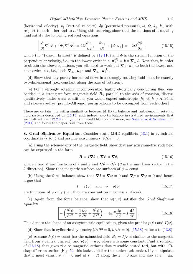
Oxford MMathPhys Lectures: Plasma Kinetics and MHD 159
(horizontal velocity), u‖ (vertical velocity), δp (perturbed pressure), ω, Ω, k‖, k⊥ withrespect to each other and to ε. Using this ordering, show that the motions of a rotatingfluid satisfy the following reduced equations
∂
∂t∇2⊥Φ+
Φ,∇2
⊥Φ
= 2Ω∂u‖
∂z,
∂u‖
∂t+Φ, u‖
= −2Ω
∂Φ
∂z, (15.15)
where the “Poisson bracket” is defined by (12.110) and Φ is the stream function of the
perpendicular velocity, i.e., to the lowest order in ε, u(0)⊥ = z×∇⊥Φ. Note that, in order
to obtain the above equations, you will need to work out ∇⊥ ·u⊥ to both the lowest and
next order in ε, i.e., both ∇⊥ · u(0)⊥ and ∇⊥ · u(1)
⊥ .
(d) Show that any purely horizontal flows in a strongly rotating fluid must be exactlytwo-dimensional (i.e., constant along the axis of rotation).
(e) For a strongly rotating, incompressible, highly electrically conducting fluid em-bedded in a strong uniform magnetic field B0 parallel to the axis of rotation, discussqualitatively under what conditions you would expect anisotropic (k‖ k⊥) Alfvenicand slow-wave-like (pseudo-Alfvenic) perturbations to be decoupled from each other?
There are certain interesting similarities between MHD turbulence and turbulence in rotatingfluid systems described by (15.15) and, indeed, also turbulence in stratified environments thatwe dealt with in §12.2.8 and Q5. If you would like to know more, see Nazarenko & Schekochihin(2011) and follow the paper trail from there.
8. Grad–Shafranov Equation. Consider static MHD equilibria (13.1) in cylindricalcoordinates (r, θ, z) and assume axisymmetry, ∂/∂θ = 0.
(a) Using the solenoidality of the magnetic field, show that any axisymmetric such fieldcan be expressed in the form
B = I∇θ + ∇ψ ×∇θ, (15.16)
where I and ψ are functions of r and z and ∇θ = θ/r (θ is the unit basis vector in theθ direction). Show that magnetic surfaces are surfaces of ψ = const.
(b) Using the force balance, show that ∇I ×∇ψ = 0 and ∇p ×∇ψ = 0 and henceargue that
I = I(ψ) and p = p(ψ) (15.17)
are functions of ψ only (i.e., they are constant on magnetic surfaces).
(c) Again from the force balance, show that ψ(r, z) satisfies the Grad–Shafranovequation
−(∂2ψ
∂r2− 1
r
∂ψ
∂r+∂2ψ
∂z2
)= 4πr2 dp
dψ+ I
dI
dψ. (15.18)
This defines the shape of an axisymmetric equilibrium, given the profiles p(ψ) and I(ψ).
(d) Show that in cylindrical symmetry (∂/∂θ = 0, ∂/∂z = 0), (15.18) reduces to (13.8).
(e) Assume I(ψ) = const (so the azimuthal field Bθ = I/r is similar to the magneticfield from a central current) and p(ψ) = aψ, where a is some constant. Find a solutionof (15.18) that gives rise to magnetic surfaces that resemble nested tori, but with “D-shaped” cross section (Fig. 59; this looks a bit like the modern tokamaks). If you stipulatethat p must vanish at r = 0 and at r = R along the z = 0 axis and also at z = ±L
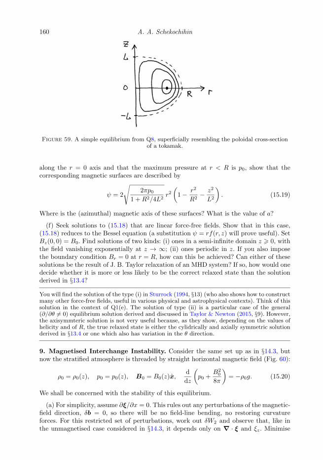
160 A. A. Schekochihin
Figure 59. A simple equilibrium from Q8, superficially resembling the poloidal cross-sectionof a tokamak.
along the r = 0 axis and that the maximum pressure at r < R is p0, show that thecorresponding magnetic surfaces are described by
ψ = 2
√2πp0
1 +R2/4L2r2
(1− r2
R2− z2
L2
). (15.19)
Where is the (azimuthal) magnetic axis of these surfaces? What is the value of a?
(f) Seek solutions to (15.18) that are linear force-free fields. Show that in this case,(15.18) reduces to the Bessel equation (a substitution ψ = rf(r, z) will prove useful). SetBz(0, 0) = B0. Find solutions of two kinds: (i) ones in a semi-infinite domain z > 0, withthe field vanishing exponentially at z → ∞; (ii) ones periodic in z. If you also imposethe boundary condition Br = 0 at r = R, how can this be achieved? Can either of thesesolutions be the result of J. B. Taylor relaxation of an MHD system? If so, how would onedecide whether it is more or less likely to be the correct relaxed state than the solutionderived in §13.4?
You will find the solution of the type (i) in Sturrock (1994, §13) (who also shows how to constructmany other force-free fields, useful in various physical and astrophysical contexts). Think of thissolution in the context of Q1(e). The solution of type (ii) is a particular case of the general(∂/∂θ 6= 0) equilibrium solution derived and discussed in Taylor & Newton (2015, §9). However,the axisymmteric solution is not very useful because, as they show, depending on the values ofhelicity and of R, the true relaxed state is either the cylidrically and axially symmetric solutionderived in §13.4 or one which also has variation in the θ direction.
9. Magnetised Interchange Instability. Consider the same set up as in §14.3, butnow the stratified atmosphere is threaded by straight horizontal magnetic field (Fig. 60):
ρ0 = ρ0(z), p0 = p0(z), B0 = B0(z)x,d
dz
(p0 +
B20
8π
)= −ρ0g. (15.20)
We shall be concerned with the stability of this equilibrium.
(a) For simplicity, assume ∂ξ/∂x = 0. This rules out any perturbations of the magnetic-field direction, δb = 0, so there will be no field-line bending, no restoring curvatureforces. For this restricted set of perturbations, work out δW2 and observe that, like inthe unmagnetised case considered in §14.3, it depends only on ∇ · ξ and ξz. Minimise
Oxford MMathPhys Lectures: Plasma Kinetics and MHD 161
Figure 60. Magnetised atmosphere.
δW2 with respect to ∇ · ξ and show that
d
dzlnp0
ργ0+
2
β
d
dzlnB0
ρ0< 0 (15.21)
is a sufficient condition for instability (the magnetised interchange instability). Wouldyou be justified in expecting stability if the condition (15.21) were not satisfied?
(b) Explain how this instability operates and rederive the condition for instability byconsidering interchanging blobs (or, rather, flux tubes), in the spirit of §14.3.3.
If field-line bending is allowed (∂ξ/∂x 6= 0), another instability emerges, the Parker (1966)instability. Do investigate.
10. Stability of the θ Pinch. Consider the following cylindrically and axially symmet-ric equilibrium:
B0 = B0(r)z, j0 = j0(r)θ = − c
4πB′0(r)θ,
d
dr
(p0 +
B20
8π
)= 0 (15.22)
(a θ pinch; see §13.1.1, Fig. 50). Consider general displacements of the form
ξ = ξmk(r)eimθ+ikz. (15.23)
Show that the θ pinch is always stable. Specifically, you should be able to show that
δW2 = πLz
∫ ∞0
dr r
γp0|∇ · ξ|2 +
B20
4π
[k2(|ξr|2 + |ξθ|2
)+
∣∣∣∣ξrr +∂ξr∂r
+imξθr
∣∣∣∣2]
> 0,
(15.24)where Lz is the length of the cylinder.
162 A. A. Schekochihin
Acknowledgments
I am grateful to many at Oxford who have given advice, commented, pointed outerrors, asked challenging questions and generally helped me get a grip. Particular thanksto Andre Lukas and Fabian Essler, who were comrades in arms in the creation ofthe MMathPhys programme, to Paul Dellar and James Binney, with whom I havecollaborated on teaching Kinetic Theory and MHD, and to Felix Parra and Peter Norreys,who have helped design a coherent sequence of courses on plasma physics.
I am also grateful to M. Kunz and to the students who took the course, amongst themT. Adkins, R. Cooper, J. Graham, C. Hamilton, M. Hardman, M. Hawes, D. Hosking,P. Ivanov and G. Wagner, for critical comments and spotting lapses in these notes. Morebroadly, I am in debt to the students who have soldiered on through these lectures and,sometimes verbally, sometimes not, projected back at me some sense of whether I wassucceeding in communicating what I wanted to communicate.
My exposition was greatly influenced by the Princeton lectures by Russell Kulsrud(on MHD; now published: Kulsrud 2005) and the UCLA ones by Steve Cowley (Cowley2004), as well as by the excellent books of Kadomtsev (1965), Krall & Trivelpiece (1973),Alexandrov et al. (1984) and Kingsep (2004).
Section 5 appeared as a result of G. Lesur’s invitation to lecture on plasma stabilityat the 2017 Les Houches School on Plasma Physics—forcing me to face the challengeof teaching something fundamental, beautiful, but not readily available in every plasmacourse. I owe §8 to Toby Adkins, who sorted much of it out in his MMathPhys dissertation(Adkins 2018).
Appendix A. Kolmogorov Turbulence
When I fill up this section, it will be an updated version of my lectures that, inhandwritten form, can be found here: http://www-thphys.physics.ox.ac.uk/people/AlexanderSchekochihin/notes/SummerSchool07/. In the meanwhile, §§33-34 of Lan-dau & Lifshitz (1987) contain almost everything you need to know, but if you want toknow more, books by Frisch (1995) and Davidson (2004) are modern classics that onecannot go wrong by reading.
In a somewhat lateral way, the scientific biography of Robert Kraichnan by Eyink &Frisch (2010) is an excellent read about turbulence, putting the subject (or at least itsantecedents) in a broader context of theoretical physics and containing very many relevantreferences (especially early ones). These authors are not, however, quite as broad-mindedor (in my view) up to date as I would have liked on the subject of intermittency, evenin their contextual referencing. My favorite intermittency (in MHD) paper is, obviously,Mallet & Schekochihin (2017), whence you can follow the references back in time (or lookinstead at the last of the 5 lectures linked above).
A.1. Dimensional Theory of the Kolmogorov Cascade
A.2. Exact Laws
A.3. Intermittency
A.4. Turbulent Mixing
REFERENCES
Abel, I. G., Plunk, G. G., Wang, E., Barnes, M., Cowley, S. C., Dorland, W.

Oxford MMathPhys Lectures: Plasma Kinetics and MHD 163
& Schekochihin, A. A. 2013 Multiscale gyrokinetics for rotating tokamak plasmas:fluctuations, transport and energy flows. Rep. Prog. Phys. 76, 116201.
Adams, D. 1979 The Hitch-Hiker’s Guide to the Galaxy . London: Pan Books.
Adkins, T. 2018 Relaxation and nonlinearity: the phase-space dynamics of Vlasov-kineticplasmas. MMathPhys Thesis. University of Oxford.
Adkins, T. & Schekochihin, A. A. 2018 A solvable model of Vlasov-kinetic plasma turbulencein Fourier-Hermite phase space. J. Plasma Phys. 84, 905840107.
Alexandrov, A. F., Bogdankevich, L. S. & Rukhadze, A. A. 1984 Principles of PlasmaElectrodynamics. Berlin: Springer.
Arnold, V. I. & Khesin, B. A. 1999 Topological Methods in Hydrodynamics. Berlin: Springer.
Balbus, S. A. 2015 Astrophysical Fluid Dynamics. Lecture Notes for the Oxford MMathPhyscourse; URL: https://www2.physics.ox.ac.uk/contacts/people/balbus.
Balbus, S. A. & Hawley, J. F. 1991 A powerful local shear instability in weakly magnetizeddisks. I. Linear analysis. Astrophys. J. 376, 214.
Balescu, R. 1963 Statistical Mechanics of Charged Particles. New York: Interscience Press.
Bedrossian, J. 2016 Nonlinear echoes and Landau damping with insufficient regularity.arXiv:1605.06841.
Bernstein, I. B. 1958 Waves in a plasma in a magnetic field. Phys. Rev. 109, 10.
Bernstein, I. B., Frieman, E. A., Kruskal, M. D. & Kulsrud, R. M. 1958 An energyprinciple for hydromagnetic stability problems. Proc. R. Soc. London A 244, 17.
Besse, N., Elskens, Y., Escande, D. F. & Bertrand, P. 2011 Validity of quasilinear theory:refutations and new numerical confirmation. Plasma Phys. Control. Fusion 53, 025012.
Binney, J. J. 2016 Kinetic Theory of Self-Gravitating Systems. Lecture Notes for the OxfordMMathPhys course on Kinetic Theory; URL: http://www-thphys.physics.ox.ac.uk/user/JamesBinney/kt.pdf.
Bohm, D. & Gross, E. P. 1949a Theory of plasma oscillations. A. Origin of medium-likebehavior. Phys. Rev. 75, 1851.
Bohm, D. & Gross, E. P. 1949b Theory of plasma oscillations. B. Excitation and damping ofoscillations. Phys. Rev. 75, 1864.
Boldyrev, S., Horaites, K., Xia, Q. & Perez, J. C. 2013 Toward a theory of astrophysicalplasma turbulence at subproton scales. Astrophys. J. 777, 41.
Braginskii, S. I. 1965 Transport processes in a plasma. Rev. Plasma Phys. 1, 205.
Buneman, O. 1958 Instability, turbulence, and conductivity in current-carrying plasma. Phys.Rev. Lett. 1, 8.
Case, K. M. 1959 Plasma oscillations. Ann. Phys. (N.Y.) 7, 349.
Chandrasekhar, S. 2003 Hydrodynamic and Hydromagnetic Stability . Dover.
Chapman, S. & Cowling, T. G. 1991 The Mathematical Theory of Non-Uniform Gases.Cambridge: Cambridge University Press, 3rd Edition.
Chew, G. F., Goldberger, M. L. & Low, F. E. 1956 The Boltzmann equation and the one-fluid hydromagnetic equations in the absence of particle collisions. Proc. R. Soc. London A236, 112.
Connor, J. W., Hastie, R. J. & Taylor, J. B. 1979 High mode number stability of anaxisymmetric toroidal plasma. Proc. R. Soc. London A 365, 1.
Cowley, S. C. 2004 Plasma Physics. Lecture Notes for the UCLA course; URL: http://www-thphys.physics.ox.ac.uk/research/plasma/CowleyLectures/.
Cowley, S. C. & Artun, M. 1997 Explosive instabilities and detonation inmagnetohydrodynamics. Phys. Rep. 283, 185.
Cowley, S. C., Cowley, B., Henneberg, S. A. & Wilson, H. R. 2015 Explosive instabilityand erupting flux tubes in a magnetized plasma. Proc. R. Soc. London A 471, 20140913.
Davidson, P. A. 2004 Turbulence: An Introduction for Scientists and Engineers. Oxford: OxfordUniversity Press.
Davidson, P. A. 2016 Introduction to Magnetohydrodynamics (2nd edition). Cambridge:Cambridge University Press.
Davidson, R. C. 1983 Kinetic waves and instabilities in a uniform plasma. In Handbook ofPlasma Physics, Volume 1 (ed. A. A. Galeev & R. N. Sudan), p. 519. Amsterdam: North-Holland.

164 A. A. Schekochihin
Dellar, P. J. 2015 Kinetic Theory of Gases. Lecture Notes for the Oxford MMathPhys courseon Kinetic Theory; URL: http://people.maths.ox.ac.uk/dellar/MMPkinetic.html.
Dellar, P. J. 2017 Hydrodynamics of Complex Fluids. Lecture Notes for the OxfordMMathPhys course on Advanced Fluid Dynamics; URL: http://people.maths.ox.ac.uk/dellar/MMP_Non_Newt_fluids.html.
Diamond, P. H., Itoh, S.-I. & Itoh, K. 2010 Modern Plasma Physics. Volume 1: PhysicalKinetics of Turbulent Plasmas. Cambridge: Cambridge University Press.
Drummond, W. E. & Pines, D. 1962 Nonlinear stability of plasma oscillations. Nucl. FusionSuppl., Part 3 p. 1049.
DuBois, D. F., Russell, D. & Rose, H. A. 1995 Reduced description of strong Langmuirturbulence from kinetic theory. Phys. Plasmas 2, 76.
Dupree, T. H. 1972 Theory of phase space density granulation in plasma. Phys. Fluids 15,334.
Elsasser, W. M. 1950 The hydromagnetic equations. Phys. Rev. 79, 183.
Eyink, G. & Frisch, U. 2010 Robert H. Kraichnan. arXiv:1011.2383.
Fowler, T. K. 1963 Lyapunov’s stability criteria for plasmas. J. Math. Phys. 4, 559.
Fowler, T. K. 1964 Bounds on plasma instability growth rates. Phys. Fluids 7, 249.
Fowler, T. K. 1968 Thermodynamics of unstable plasmas. In Advances in Plasma Physics(ed. A. Simon & W. B. Thompson), , vol. 1, p. 201. New York: Interscience Press.
Fowler, T. K. 2016 Speculations about plasma free energy, 50 years later. J. Plasma Phys.82, 925820501.
Freidberg, J. 2014 Ideal MHD . Cambridge: Cambridge University Press.
Fried, B. D. & Conte, S. D. 1961 The Plasma Dispersion Function. New York: AcademicPress.
Frisch, U. 1995 Turbulence: The Legacy of A. N. Kolmogorov . Cambridge: CambridgeUniversity Press.
Furth, H. P., Killeen, J. & Rosenbluth, M. N. 1963 Finite-resistivity instabilities of asheet pinch. Phys. Fluids 6, 459.
Gardner, C. S. 1963 Bound on the energy available from a plasma. Phys. Fluids 6, 839.
Goedbloed, H. & Poedts, S. 2004 Principles of Magnetohydrodynamics. Cambridge:Cambridge University Press.
Goldman, M. V. 1984 Strong turbulence of plasma waves. Rev. Mod. Phys. 56, 709.
Gould, R. W., O’Neil, T. M. & Malmberg, J. H. 1967 Plasma wave echo. Phys. Rev. Lett.19, 219.
Haeff, A. 1949 The electron-wave tube—a novel method of generation and amplification ofmicrowave energy. Proc. IRE 37, 4.
Haines, M. G. 2011 A review of the dense Z-pinch. Plasma Phys. Control. Fusion 53, 093001.
Helander, P. 2017 Available energy and ground states of collisionless plasmas. J. Plasma Phys.83, 715830401.
Helander, P. & Sigmar, D. J. 2005 Collisional Transport in Magnetized Plasmas. Cambridge:Cambridge University Press.
Heninger, J. M. & Morrison, P. J. 2018 An integral transform technique for kinetic systemswith collisions. Phys. Plasmas 25, 082118.
Howes, G. G., Cowley, S. C., Dorland, W., Hammett, G. W., Quataert, E. &Schekochihin, A. A. 2006 Astrophysical gyrokinetics: basic equations and linear theory.Astrophys. J. 651, 590.
Jackson, J. D. 1960 Longitudinal plasma oscillations. J. Nuclear Energy C 1, 171.
Kadomtsev, B. B. 1965 Plasma Turbulence. Academic Press.
Kadomtsev, B. B. & Pogutse, O. P. 1970 Collisionless relaxation in systems with Coulombinteractions. Phys. Rev. Lett. 25, 1155.
Kadomtsev, B. B. & Pogutse, O. P. 1971 Theory of beam-plasma interaction. Phys. Fluids14, 2470.
Kadomtsev, B. B. & Pogutse, O. P. 1974 Nonlinear helical perturbations of a plasma in thetokamak. Sov. Phys.–JETP 38, 575.
Kanekar, A., Schekochihin, A. A., Dorland, W. & Loureiro, N. F. 2015 Fluctuation-

Oxford MMathPhys Lectures: Plasma Kinetics and MHD 165
dissipation relations for a plasma-kinetic Langevin equation. J. Plasma Phys. 81,305810104.
Kingsep, A. S. 2004 Introduction to Nonlinear Plasma Physics. Moscow: MZ Press (in Russian).
Kingsep, A. S., Rudakov, L. I. & Sudan, R. N. 1973 Spectra of strong Langmuir turbulence.Phys. Rev. Lett. 31, 1482.
Klimontovich, Yu. L. 1967 The Statistical Theory of Non-Equilibrium Processes in a Plasma.MIT Press.
Kolmogorov, A. N. 1941 The local structure of turbulence in incompressible viscous fluid atvery large Reynolds numbers. Dokl. Acad. Nauk SSSR 30, 299.
Krall, N. A. & Trivelpiece, A. W. 1973 Principles of Plasma Physics. New York: McGraw-Hill.
Krommes, J. A. 2015 A tutorial introduction to the statistical theory of turbulent plasmas, ahalf-century after Kadomtsev’s Plasma Turbulence and the resonance-broadening theoryof Dupree and Weinstock. J. Plasma Phys. 81, 205810601.
Krommes, J. A. 2018 Projection-operator methods for classical transport in magnetizedplasmas. Part I. Linear response, the Braginskii equations and fluctuating hydrodynamics.J. Plasma Phys. 84, 925840401.
Kruskal, M. D. & Oberman, C. R. 1958 On the stability of plasma in static equilibrium.Phys. Fluids 1, 275.
Kulsrud, R. M. 1983 MHD description of plasma. In Handbook of Plasma Physics, Volume 1(ed. A. A. Galeev & R. N. Sudan), p. 1. Amsterdam: North-Holland.
Kulsrud, R. M. 2005 Plasma Physics for Astrophysics. Princeton: Princeton University Press.
Kunz, M. W., Abel, I. G., Klein, K. G. & Schekochihin, A. A. 2018 Astrophysicalgyrokinetics: turbulence in pressure-anisotropic plasmas at ion scales and beyond.J. Plasma Phys., in press; E-print arXiv:1712.02269.
Kunz, M. W., Schekochihin, A. A., Chen, C. H. K., Abel, I. G. & Cowley, S. C. 2015Inertial-range kinetic turbulence in pressure-anisotropic astrophysical plasmas. J. PlasmaPhys. 81, 325810501.
Landau, L. 1936 Transport equation in the case of Coulomb interaction. Zh. Eksp. Teor. Fiz.7, 203.
Landau, L. 1946 On the vibration of the electronic plasma. Zh. Eksp. Teor. Fiz. 16, 574, Englishtranslation: J. Phys. USSR 10, 25 (1946).
Landau, L. D. & Lifshitz, E. M. 1976 Mechanics (L. D. Landau and E. M. Lifshitz’s Courseof Theoretical Physics, Volume 1). Butterworth–Heinemann.
Landau, L. D. & Lifshitz, E. M. 1987 Fluid Mechanics (L. D. Landau and E. M. Lifshitz’sCourse of Theoretical Physics, Volume 6). Oxford: Pergamon Press.
Lifshitz, E. M. & Pitaevskii, L. P. 1981 Physical Kinetics (L. D. Landau and E. M. Lifshitz’sCourse of Theoretical Physics, Volume 10). Elsevier.
Loureiro, N. F., Schekochihin, A. A. & Cowley, S. C. 2007 Instability of current sheetsand formation of plasmoid chains. Phys. Plasmas 14, 100703.
Mallet, A. & Schekochihin, A. A. 2017 A statistical model of three-dimensional anisotropyand intermittency in strong Alfvenic turbulence. Mon. Not. R. Astron. Soc. 466, 3918.
Malmberg, J. H. & Wharton, C. B. 1964 Collisionless damping of electrostatic plasma waves.Phys. Rev. Lett. 13, 184.
Malmberg, J. H., Wharton, C. B., Gould, R. W. & O’Neil, T. M. 1968 Plasma waveecho experiment. Phys. Rev. Lett. 20, 95.
Mazitov, R. K. 1965 Damping of plasma waves. J. Appl. Mech. Tech. Phys. 6, 22.
Moffatt, H. K. 1978 Magnetic Field Generation in Electrically Conducting Fluids. Cambridge:Cambridge University Press.
Morrison, P. 2000 Hamiltonian description of Vlasov dynamics: Action-angle variables for thecontinuous spectrum. Transport Theory Stat. Phys. 29, 397.
Morrison, P. J. 1994 The energy of perturbations for Vlasov plasmas. Phys. Plasmas 1, 1447.
Musher, S. L., Rubenchik, A. M. & Zakharov, V. E. 1995 Weak Langmuir turbulence.Phys. Rep. 252, 177.
Nazarenko, S. 2011 Wave Turbulence. Berlin: Springer.
Nazarenko, S. V. & Schekochihin, A. A. 2011 Critical balance in magnetohydrodynamic,

166 A. A. Schekochihin
rotating and stratified turbulence: towards a universal scaling conjecture. J. Fluid Mech.677, 134.
Newcomb, W. A. 1962 Lagrangian and Hamiltonian methods in magnetohydrodynamics.Nuclear Fusion: Supplement, Part 2 p. 451.
Nyquist, H. 1932 Regeneration theory. Bell Syst. Tech. J. 11, 126.Ogilvie, G. I. 2016 Astrophysical fluid dynamics. J. Plasma Phys. 82, 205820301.Ogilvie, G. I. & Proctor, M. R. E. 2003 On the relation between viscoelastic and
magnetohydrodynamic flows and their instabilities. J. Fluid Mech. 476, 389.O’Neil, T. 1965 Collisionless damping of nonlinear plasma oscillations. Phys. Fluids 8, 2255.Parker, E. N. 1966 The dynamical state of the interstellar gas and field. Astrophys. J. 145,
811.Parra, F. I. 2018a Collisional Plasma Physics. Lecture Notes for an Oxford
MMathPhys course; URL: http://www-thphys.physics.ox.ac.uk/people/FelixParra/\CollisionalPlasmaPhysics/CollisionalPlasmaPhysics.html.
Parra, F. I. 2018b Collisionless Plasma Physics. Lecture Notes for an OxfordMMathPhys course; URL: http://www-thphys.physics.ox.ac.uk/people/FelixParra/\CollisionlessPlasmaPhysics/CollisionlessPlasmaPhysics.html.
Peierls, R. E. 1955 Quantum Theory of Solids. Oxford: Clarendon Press.Pelletier, G. 1980 Langmuir turbulence as a critical phenomenon. Part 1. Destruction of the
statistical equilibrium of an interacting-modes ensemble. J. Plasma Phys. 24, 287.Penrose, O. 1960 Electrostatic instabilities of a uniform non-Maxwellian plasma. Phys. Fluids
3, 258.Pfirsch, D. & Sudan, R. N. 1993 Nonlinear ideal magnetohydrodynamics instabilities. Phys.
Fluids B 5, 2052.Pierce, J. R. & Hebenstreit, W. B. 1949 A new type of high-frequency amplifier. Bell Syst.
Tech. J. 28, 33.Ramos, J. J. & White, R. L. 2018 Normal-mode-based analysis of electron plasma waves with
second-order Hermitian formalism. Phys. Plasmas 25, 034501.Robinson, P. A. 1997 Nonlinear wave collapse and strong turbulence. Rev. Mod. Phys. 69, 507.Rudakov, L. I. & Tsytovich, V. N. 1978 Strong Langmuir turbulence. Phys. Rep. 40, 1.Ruyer, C., Gremillet, L., Debayle, A. & Bonnaud, G. 2015 Nonlinear dynamics of the
ion Weibel-filamentation instability: An analytical model for the evolution of the plasmaand spectral properties. Phys. Plasmas 22, 032102.
Sagdeev, R. Z. & Galeev, A. A. 1969 Nonlinear Plasma Theory . W. A. Benjamin.Schekochihin, A. A. 2018 Kinetic Theory and Statistical Physics. Lecture Notes for the
Oxford Physics course, Paper A1; URL: http://www-thphys.physics.ox.ac.uk/people/AlexanderSchekochihin/A1/2014/A1LectureNotes.pdf.
Schekochihin, A. A. & Cowley, S. C. 2007 Turbulence and magnetic fields in astrophysicalplasmas. In Magnetohydrodynamics: Historical Evolution and Trends (ed. S. Molokov,R. Moreau & H. K. Moffatt), p. 85. Berlin: Springer, reprint: URL: http://www-thphys.physics.ox.ac.uk/people/AlexanderSchekochihin/mhdbook.pdf.
Schekochihin, A. A., Cowley, S. C., Dorland, W., Hammett, G. W., Howes, G. G.,Quataert, E. & Tatsuno, T. 2009 Astrophysical gyrokinetics: kinetic and fluidturbulent cascades in magnetized weakly collisional plasmas. Astrophys. J. Suppl. 182,310.
Schekochihin, A. A., Cowley, S. C., Rincon, F. & Rosin, M. S. 2010 Magnetofluiddynamics of magnetized cosmic plasma: firehose and gyrothermal instabilities. Mon. Not.R. Astron. Soc. 405, 291.
Schekochihin, A. A., Parker, J. T., Highcock, E. G., Dellar, P. J., Dorland, W. &Hammett, G. W. 2016 Phase mixing versus nonlinear advection in drift-kinetic plasmaturbulence. J. Plasma Phys. 82, 905820212.
Squire, J., Schekochihin, A. A. & Quataert, E. 2017 Amplitude limits and nonlineardamping of shear-Alfven waves in high-beta low-collisionality plasmas. New J. Phys., inpress [arXiv:1701.03175].
Strauss, H. R. 1976 Nonlinear, three-dimensional magnetohydrodynamics of noncirculartokamaks. Phys. Fluids 19, 134.
Sturrock, P. A. 1966 Stochastic acceleration. Phys. Rev. 141, 186.

Oxford MMathPhys Lectures: Plasma Kinetics and MHD 167
Sturrock, P. A. 1994 Plasma Physics. An Introduction to the Theory of Astrophysical,Geophysical and Laboratory Plasmas. Cambridge: Cambridge University Press.
Taylor, J. B. & Newton, S. L. 2015 Special topics in plasma confinement. J. Plasma Phys.81, 205810501.
Thornhill, S. G. & ter Haar, D. 1978 Langmuir turbulence and modulational instability.Phys. Rep. 43, 43.
Tobias, S. M., Cattaneo, F. & Boldyrev, S. 2012 MHD dynamos and turbulence. In TenChapters in Turbulence (ed. P. A. Davidson, Y. Kaneda & K. R. Sreenivasan), p. 351.Cambridge University Press, e-print arXiv:1103.3138.
Tonks, L. & Langmuir, I. 1929 Oscillations in ionized gases. Phys. Rev. 33, 195.Tsytovich, V. N. 1995 Lectures on Non-linear Plasma Kinetics. Berlin: Springer.Uzdensky, D. A., Loureiro, N. F. & Schekochihin, A. A. 2010 Fast magnetic reconnection
in the plasmoid-dominated regime. Phys. Rev. Lett. 105, 235002.van Kampen, N. G. 1955 On the theory of stationary waves in plasmas. Physica 9, 949.van Kampen, N. G. & Felderhof, B. U. 1967 Theoretical Methods in Plasma Physics.
Amsterdam: North-Holland.Vedenov, A. A. 1963 Quasilinear plasma theory (theory of a weakly turbulent plasma). Plasma
Phys. (J. Nucl. Energy C) 5, 169.Vedenov, A. A., Velikhov, E. P. & Sagdeev, R. Z. 1962 Quasilinear theory of plasma
oscillations. Nucl. Fusion Suppl., Part 2 p. 465 (in Russian).Villani, C. 2014 Particle systems and nonlinear Landau damping. Phys. Plasmas 21, 030901.Weibel, E. S 1958 Spontaneously growing transverse waves in a plasma due to an anisotropic
velocity distribution. Phys. Rev. Lett. 2, 83.Wicks, R. T., Roberts, D. A., Mallet, A., Schekochihin, A. A., Horbury, T. S. &
Chen, C. H. K. 2013 Correlations at large scales and the onset of turbulence in the fastsolar wind. Astrophys. J. 778, 177.
Zakharov, V. E. 1972 Collapse of Langmuir waves. Sov. Phys.–JETP 35, 908.Zakharov, V. E., Lvov, V. S. & Falkovich, G. 1992 Kolmogorov Spectra of Turbulence I:
Wave Turbulence. Berlin: Springer (updated online version URL: https://www.weizmann.ac.il/chemphys/lvov/research/springer-series-nonlinear-dynamics).
Zakharov, V. E., Musher, S. L. & Rubenchik, A. M. 1985 Hamiltonian approach to thedescription of non-linear plasma phenomena. Phys. Rep. 129, 285.
Zeldovich, Ya. B. 1956 The magnetic field in the two-dimensional motion of a conductingturbulent liquid. Zh. Eksp. Teor. Fiz. 31, 154, English translation: Sov. Phys. JETP 4,460 (1957).
Zhdankin, V., Boldyrev, S. & Uzdensky, D. A. 2016 Scalings of intermittent structures inmagnetohydrodynamic turbulence. Phys. Plasmas 23, 055705.
Ziman, J. M. 1960 Electrons and Phonons: The Theory of Transport Phenomena in Solids.Oxford: Clarendon Press.