Embed Size (px)
Citation preview

LED Light Control for use in
Visible Light Communications
A Degree Thesis
Submitted to the Faculty of the
Escola Tècnica d'Enginyeria de Telecomunicació de
Barcelona
Universitat Politècnica de Catalunya
by
Carlos Labella
In partial fulfilment
of the requirements for the degree in
ELECTRONICS SYSTEM ENGINEERING
Advisor: Prof. Josep Paradells Aspas
Barcelona, May 2017


Abstract
This project describes the implementation of a custom LED driver based on the Texas
Instruments TPS92641 integrated circuit. The main contribution of this project is to show
how a generic driver for LED luminaires can obtain a data communication rate of up to 133
kbps when placed up to 3 meters away from the corresponding receiver. This document
provides both an evaluation of the data converter, based on a MAX79356 modem designed
for Power Line Communications, and the corresponding throughput evaluations when
employing this chip for Visual Light Communication (VLC) purposes.

Resum
L’objecte d’investigació d’aquest projecte és la implementació d'un controlador per
lluminàries LED comercials basat en un circuit integrat TPS92641 de Texas Instruments.
La principal contribució d’aquest estudi rau en demostrar que, fent ús d'un controlador
genèric per lluminàries LED, és possible obtenir una comunicació de dades de fins a 133
kbps a una distància de 3 metres. L'estudi se centra en avaluar el comportament del
convertidor i la realització de demostracions de rendiment. Entre d'altres, s'avalua l'ús del
component MAX79356, un mòdem per a Power Line Communications, i es demostra com
es pot emprar satisfactòriament per a comunicacions per llum visible (VLC).

Resumen
El objeto de investigación de este proyecto es la implementación de un controlador basado
en un circuito integrado TPS92641 de Texas Instruments para luminarias LED comerciales.
La principal contribución de este proyecto es demostrar que, haciendo uso de un
controlador genérico para luminarias LED, es posible obtener una tasa de transferencia de
133 kbps a una distancia de 3 metros. El estudio se centra en evaluar el comportamiento
del convertidor y en la realización de demostraciones de rendimiento. Entre otros, se
evalúa el uso del componente MAX79356, un modem para Power Line Communications
(PLC) y se demuestra su uso satisfactorio en el campo de las comunicaciones por luz
visible (VLC).

I am grateful to, my father, Luis Manuel, for being a reference for me along my life, both in personal and professional fields, my mother, Maria, for making easier everyday task and encourage my academic career, my brothers, Daniel and Juan Luis, for their unconditional support and help in different stages of the project.
Especially, I thank my girlfriend, Gisela, for being able to show me the good side of things.
This project is so mine as your.
Agradezco, a mi padre, Luis Manuel, por haber sido una referencia para mí a lo largo de mi vida, tanto en el ámbito personal como profesional, a mi madre, María, por facilitarme tareas del día a día y la dedicación a los estudios, a mis hermanos, Daniel y Juan Luis, por su apoyo incondicional y su ayuda en varias etapas del proyecto.
De manera especial, agradezco a mi pareja, Gisela, por ser capaz de mostrarme el lado bueno de las cosas.
Este proyecto es tan mío como vuestro.

Acknowledgements
I thank my Thesis’ advisor, Dr. Josep Paradells, his invaluable help along this project. Also,
I thank Dr. Joaquim Oller, for his help in different stages of the development.


Revision history and approval record
Revision Date Purpose
0 14/04/2017 Document creation
1 17/04/2017 Document revision
2 23/04/2017 Document revision
3 25/04/2017 Document revision
4 29/04/2017 Document revision
5 1/05/2017 Document revision
6 3/05/2017 Document revision
7 8/05/2017 Document revision
8 11/05/2017 Document revision
9 14/05/2017 Document revision
DOCUMENT DISTRIBUTION LIST
Name e-mail
Carlos Labella [email protected]
Josep Paradells [email protected]
Written by: Reviewed and approved by:
Date 14/04/2017 Date 15/05/2017
Name Carlos Labella Name Josep Paradells
Position Project Author Position Project Supervisor


Table of contents
Abstract ............................................................................................................................ 2
Resum .............................................................................................................................. 3
Resumen .......................................................................................................................... 4
Acknowledgements .......................................................................................................... 6
Revision history and approval record ................................................................................ 8
Table of contents ............................................................................................................ 10
List of Figures ................................................................................................................. 12
List of Tables .................................................................................................................. 16
1. Introduction ................................................................................................................ 1
1.1. Statement of purpose ......................................................................................... 1
1.2. Requirements and specification .......................................................................... 2
1.3. Methods and procedures .................................................................................... 3
1.4. Work plan ........................................................................................................... 3
1.5. Deviations from initial plan .................................................................................. 4
2. State of the Art .......................................................................................................... 6
2.1. White LED vs RGB LED ..................................................................................... 7
2.2. Buck converter control topologies ....................................................................... 9
2.2.1. Voltage mode control ................................................................................... 9
2.2.2. Current mode control ................................................................................. 10
2.2.3. Hysteresis (ripple) control .......................................................................... 10
3. Project development: ............................................................................................... 12
3.1. Buck converter for LED driver selection ............................................................ 12
3.2. TPS92641 specification .................................................................................... 14
3.3. TPS92641EVM mods ....................................................................................... 14
3.4. Hands-on experience with TPS92641EVM ....................................................... 17
3.4.1. Bandwidth measurement ........................................................................... 18
3.4.2. Commercial lamps compatibility test .......................................................... 24
4. Applications ............................................................................................................. 26
4.1. Baseband Audio over VLC ............................................................................... 26
4.1.1. LED driver control input adaption for baseband audio signal. .................... 26
4.1.2. Baseband Audio over VLC receiver ........................................................... 29
4.1.3. Conclusions of implemented application .................................................... 33
4.2. FM Audio over VLC .......................................................................................... 33

4.2.1. Frequency modulation implementation ...................................................... 34
4.2.2. Frequency demodulation implementation .................................................. 37
4.2.2.1. VLC receiver ........................................................................................... 37
4.2.3. CD4046B configuration for FM demodulation ............................................ 43
4.2.4. Conclusions of implemented application .................................................... 45
4.3. OFDM VLC based system evaluation ............................................................... 46
4.3.1. G3-PLC technology ................................................................................... 46
4.3.2. MAX79356 ................................................................................................ 47
4.3.2.1. Simple MAC firmware evaluation ............................................................. 52
4.3.2.2. Full MAC firmware ................................................................................... 58
4.3.2.3. Transparent UART firmware .................................................................... 59
4.4. Custom modulation evaluation.......................................................................... 59
4.4.1. Custom modulation transmitter design....................................................... 60
4.4.2. Custom modulation receiver design ........................................................... 64
4.4.3. Conclusions of implemented application .................................................... 70
5. Budget ..................................................................................................................... 71
5.1. VLC LED driver ................................................................................................ 71
5.2. VLC Receiver ................................................................................................... 72
5.3. Baseband Audio VLC application ..................................................................... 73
5.4. FM Audio VLC application ................................................................................ 74
5.5. PLC VLC application ........................................................................................ 75
5.6. Custom modulation application ......................................................................... 76
5.7. Summary of total human resource dedication and cost .................................... 77
6. Conclusions and Future Work .................................................................................. 78
Bibliography .................................................................................................................... 81
Appendices ..................................................................................................................... 83
Glossary ....................................................................................................................... 103

List of Figures
Figure 1. Project scheduling Gantt diagram. ..................................................................... 4
Figure 2. Visible spectrum wavelength distribution [4]. ...................................................... 7
Figure 3. Spectrum of a white LED showing blue light directly emitted by the GaN-based
LED (peak at about 465 nm) and the more broadband Stokes-shifted light emitted by the
Ce3+:YAG phosphor, which emits at roughly 500–700 nm [3]. ......................................... 8
Figure 4. Typical color-filtered transmission spectrums illustrate how the RGB-LED
spectrum has peaks for red, green and blue. .................................................................... 8
Figure 5. Simple schematic of buck converter [10]. ........................................................... 9
Figure 6. Voltage Model Control simplified description [10]. ............................................ 10
Figure 7. Current Mode Control simplified description [10]. ............................................. 10
Figure 8. Hysteresis control illustration [10]. ................................................................... 11
Figure 9. Hysteresis Control, simplified description [10]. ................................................. 11
Figure 10. STEVAL-ILL066V1 board. ............................................................................. 13
Figure 11. TPS92641EVM board. ................................................................................... 13
Figure 12. TPS92641EVM Schematic. ........................................................................... 16
Figure 13. TPS92641EVM AC response measurement connexion diagram. .................. 18
Figure 14. TPS92641 AC Response with Ccomp = 470 nF. ........................................... 18
Figure 15. TPS92641 AC response with CCOMP = 470 nF (black) and CCOMP = 100 nF (red).
....................................................................................................................................... 20
Figure 16. TPS92641 AC response Ccomp = 470 nF (black), Ccomp = 100 nF (red), Ccomp
=1 nF (blue). ................................................................................................................... 21
Figure 17. Oscilloscope screenshot with Vin = 200 mV@100 kHz using Figure 13
equipment configuration AC-coupled. ............................................................................. 22
Figure 18. Oscilloscope screenshot with Vin = 200 mV@100 kHz using Figure 13
equipment configuration DC-coupled. ............................................................................. 22
Figure 19. Oscilloscope screenshot with FFT representation of indirect LED current
measurement through RCS. Marker “S” is placed at 96 kHz and marker “E” at 846 kHz. . 23
Figure 20. Oscilloscope screenshot with FFT representation of indirect LED current
measurement through RCS. Marker “S” is placed at 744 kHz and marker “E” at 945 kHz.24
Figure 21. LED driver control input adaptation for audio signal. ...................................... 26
Figure 22. Frequency response of control adaption design for audio signals. ................. 27
Figure 23. LED driver control input adaptation for audio signal with prefiltering stage added,
fc@200 Hz. ..................................................................................................................... 28
Figure 24. Frequency response of control adaption design for audio signals with no
prefiltering (black line) and with it at fc@200Hz (red line). .............................................. 28

Figure 25. TPS92641EVM with control adaption circuit (prototype board at bottom-left
corner of the image)........................................................................................................ 29
Figure 26. Photovoltaic cell used in this project AC response. ........................................ 30
Figure 27. Audio over visible light receiver scheme. ....................................................... 30
Figure 28. Complete Baseband Audio over VLC system Frequency response. .............. 31
Figure 29. Audio over visible light reception scheme with Twin-T Notch filter.................. 31
Figure 30. Twin-T Notch filter, configuration implemented in Figure 29 , with center
frequency at 100 Hz AC response. ................................................................................. 32
Figure 31. Oscilloscope screenshot measuring fluorescent interference, CH1 received
signal on photovoltaic cell, CH2 notch filter output. ......................................................... 32
Figure 32. Audio over visible light receiver prototype. ..................................................... 33
Figure 33. CD4046B internal block diagram. .................................................................. 34
Figure 34. CD4046B diagram for audio FM modulation. ................................................. 35
Figure 35. Equipment configuration for FM application measurement. ............................ 36
Figure 36. Oscilloscope screenshot, CH1 FM signal, CH2 led current measured through
Rcs. ................................................................................................................................ 36
Figure 37. FM implementation and integrated with TPS92641EVM. ............................... 37
Figure 38. Left, OPT101 block diagram. Right, spectral responsivity. ............................. 38
Figure 39. OPT101 AC response with Rext=100 kΩ. ...................................................... 38
Figure 40. Oscilloscope screenshot, CH1 LED driver control input signal, CH2 OPT101
output signal. .................................................................................................................. 39
Figure 41. MAX9814 simplified block diagram. ............................................................... 39
Figure 42. VLC receiver diagram based and OPT101 and MAX9814. ............................ 40
Figure 43. PCB design preview image. ........................................................................... 41
Figure 44. VLC receiver based on OPT101 and MAX9814 prototype. ............................ 41
Figure 45. Equipment configuration for receiver evaluation............................................. 42
Figure 46. Oscilloscope screenshot, CH1 LED driver control input signal, CH2 Light
receiver output signal. ..................................................................................................... 42
Figure 47. FFT representation of received signal, Figure 46 CH2, Marker “S” is placed at
35 kHz, and “E” at 100 kHz. ............................................................................................ 43
Figure 48. CD4046B diagram for audio FM demodulation. ............................................. 44
Figure 49. FM audio through light system AC response. ................................................. 45
Figure 50. Left, VLC receiver prototype. Right, FM audio demodulation prototype. ......... 45
Figure 51. MAX79356 typical configuration. .................................................................... 48
Figure 52. Transmitter diagram with minimum configuration based on MAX79356. ........ 49
Figure 53. Receiver diagram with minimum configuration based on MAX79356. ............ 50

Figure 54. Implemented MAX79356 based transmitter. .................................................. 51
Figure 55. Implemented MAX79356 based receiver. ...................................................... 51
Figure 56. Devices configuration for evaluate Transmitter-Receiver system based on
MAX79356. ..................................................................................................................... 52
Figure 57. ZENO Simple Connect software main window. .............................................. 53
Figure 58. ZENO Simple Connect software screenshot with both transmitter, right side of
image, and receiver, left side of image, showing the highest transfer rate achieved. ...... 55
Figure 59. Oscilloscope screenshot, CH1 LED driver signal input, CH2 Light receiver output.
....................................................................................................................................... 57
Figure 60. FFT representation of PLC transmission signal at Figure 59. Marker “S” and “E”
are placed at first carrier, 35 kHz and last carrier, 90 kHz. .............................................. 57
Figure 61. First start of G3 “PLC connect” application screenshot. ................................. 58
Figure 62. G3 PLC Connect software screenshot after correctly receiving several packets
from transmitter. ............................................................................................................. 59
Figure 63. Custom modulation transmitter flow diagram. ................................................ 61
Figure 64. 8 bit R2R ladder DAC converter diagram. ...................................................... 62
Figure 65. PCB layout of implemented R2R ladder based DAC. ..................................... 62
Figure 66. Oscilloscope screenshot measuring R2R ladder based DAC output with the 4
different symbols generated. ........................................................................................... 63
Figure 67. Oscilloscope screenshot with CH1 LED driver control input, CH2 Light receiver
output. ............................................................................................................................ 63
Figure 68. TMS320f28027 transmitter based implementation with R2R ladder and
TPS92641 LED driver. .................................................................................................... 64
Figure 69. Oscilloscope screenshot, CH1 Received signal, CH2 comparator output, and
cursors show the voltatge threshold and hysteresis. ....................................................... 65
Figure 70. Oscilloscope screenshot, CH1 received signal, CH2 comparator output for
amplitude detection, cursor show the threshold configuration. ........................................ 65
Figure 71. Custom modulation receiver flow diagram ..................................................... 66
Figure 72. Oscilloscope screenshot CH1 received signal, CH2 zero-crossing detector
output. Between “S” and “E” cursors 0x3C byte is transmitted in 60 us. Red markers
corresponds to: T1=5.4us, T2=3.4us T3=6.2us T4=8.4us ............................................... 68
Figure 73. Oscilloscope screenshot, CH1 received signal, CH2 amplitude detector output.
....................................................................................................................................... 69
Figure 74. TMS320f28027 recevier based implementation with VLC receiver designed in
FM Audio over VLC application ...................................................................................... 70
Figure 75 The RIAA equalization curve for playback of vinyl records. The recording curve
performs the inverse function, reducing low frequencies and boosting high frequencies [14].
....................................................................................................................................... 79

Figure 76 Capture sequence for Delta Mode Time-Stamp With Rising and Falling Edge
Detect. .......................................................................................................................... 102

List of Tables
Table 1. Project task schedule table. ................................................................................ 3
Table 2. Available colours with wavelength range, voltage drop, and material [3]. ............ 6
Table 3. TPS92641EVM Electrical and Performance Specifications. .............................. 13
Table 4. Frequency mod involved components. .............................................................. 15
Table 5 Basic LED specification ..................................................................................... 17
Table 6. MAX79356 frequency bands standard supported.............................................. 46
Table 7. Maximum speed obtained in function of used modulation. ................................ 56
Table 8. Symbol codification table. ................................................................................. 60
Table 9. Possible transitions with associated time values, being T1 the time equivalent to
half period symbol. ......................................................................................................... 67
Table 10. VLC LED driver material cost. ......................................................................... 71
Table 11. VLC LED driver distributed task time and estimated cost. ............................... 71
Table 12. VLC Receiver material cost. ............................................................................ 72
Table 13. VLC Receiver distributed task time and estimated cost. .................................. 72
Table 14. Baseband Audio VLC application material cost. .............................................. 73
Table 15. Baseband Audio VLC application distributed task time and estimated cost. .... 73
Table 16. FM Audio VLC application material cost. ......................................................... 74
Table 17. FM Audio VLC application distributed task time and estimated cost. ............... 74
Table 18. PLC VLC application material cost. ................................................................. 75
Table 19. PLC VLC application distributed task time and estimated cost. ....................... 75
Table 20. Custom Modulation application material cost. ................................................. 76
Table 21. Custom Modulation application distributed task time and estimated cost. ....... 76
Table 22. Total human resource time dedication and estimated cost .............................. 77


1
1. Introduction
When we talk about data communication, its basic steps include the composition of the
message, the encoding of the message, the usage of a medium or channel, the signal
transmission, the signal reception, the correspondent decoding of the message and finally,
the interpretation of the message by the receiver.
Such communication, indeed, can be carried out in a large amount of different ways.
Nowadays’ technologies such as Wi-Fi, Bluetooth, GSM, LoRa, ADSL, among many others,
allow communications everybody is used to. The decision about which one to choose, shall
be given by different factors such as the distance between the transmitter and the receiver,
channel, message, etc.
This document focuses on a novel, different Visible Light Communication (VLC) technology.
This type of communication as an early example was firstly employed by navy vessels,
which used light reflectors to manage Morse code.
Recently, LED technology has replaced incandescent lamps by offering a greater energy
efficiency and life time. LED luminaires have other properties that make them perfect for
data communication. VLC can be efficiently implemented by such commercial LED
luminaries. Because of the ubiquity of such elements, VLC appears as an interesting
candidate for home and industrial data communications and, as of 2017, has great interest
among the scientific community, where it is frequently mentioned and discussed in
numerous R&D studies, papers and projects.
The rest of this document is structured as follows: Section 0 includes requirements,
purpose and methods for this project. Section 2 contains information about the current
state-of-the-art of VLC technology and some control methods for LED drivers. Next,
Section 3 introduces the integrated circuits which are used in Section 4, which contains
several implementations of prototypes and applications. Finally, Section 5 considers the
cost of implementing each of these applications in a realistic manner. Section 6 concludes
the document by stating several ideas for future developments.
1.1. Statement of purpose
To accomplish the development of a driver for LED light control for use in VLC, the project’s
main goals are:
1. Operate the LED driver by following an analog signal at an AC frequency of 100
kHz.
2. Demonstrate that LED driver can support an OFDM modulation (1 - 100 kHz BW).
3. Make the whole system compatible with as many lamps types as possible for it to
be applicable to real-life cases outside the laboratory.

2
1.2. Requirements and specification
Once established project main goals, project requirements and project specification are as
follow.
Project requirements:
- 1 W to 100 W LED lamp support.
There are plenty of lamp types available in market. LED lamps are often made by
a set of small LEDs in series. Normally, the number and type of LEDs determinates
the voltage and power of the lamps. To support as many lights as possible, it is
needed to have a big range in power requirement. 1 W to 100 W is enough to
support 80% of lamps present in market.
- 7 V to 60 V input voltage support.
In the most frequent use case, lamps come with its own converter, so the idea is to
do not deploy a custom one, and make possible to work with it.
- Analog modulation support.
A modulation is needed to employ light for communication purposes. On-Off-Keying
is an easy one to implement by adding an external switch that turns on and off the
LED, but also the one offering the lowest channel performance. Quadrature Phase-
Shift Keying (QPSK), an analog modulation, is more difficult to implement, but in
turn offers a better channel performance.
- 100:1 dimming ratio.
A good dimming ratio allows adjusting light intensity to different places or scenarios.
With a 100:1 ratio, there are 100 possible brightness steps between the brightest
and the darkest level.
In order to develop the project with the previous requirements, commercial parts are used
and their specifications are:
- TPS92641 led driver IC.
This integrated circuit is a synchronous buck controller for precision dimming LED
driver. It allows handling high power lamps with a voltage input range from 7 V to
85 V. Analog and digital dimming inputs are intended to be used as modulation
control signals.
- MAX79356 PLC modem.
ZENO (MAX79356) is a programmable narrowband orthogonal frequency division
multiplexing (OFDM)-based PLC modem system-on-chip (SoC) device that
provides secured power line communication in a small package.
- Power supply.
All the above elements need a voltage/current source. Both power supplies types,
one provided by LED manufacturer and one generic are employed in our tests.
Other design parts operate with battery power.

3
1.3. Methods and procedures
This project is based on a previous one made at university. The previous project consisted
in bidirectional visible light communication for a single LED lamp model, using OOK
modulation. There was a need to update and re-design the hardware so a much wider
range of LED lamps could be used as VLC transmitters and support analog modulations.
The current project aims to achieve such design and even improve the throughput of the
previous work.
1.4. Work plan
The planning of this project has been done on weekdays, with an average of 4 hours per
day. The Table 1 shows the breakdown of tasks and duration grouped by work packages.
Table 1. Project task schedule table.

4
Figure 1 shows the project scheduling Gantt diagram.
Figure 1. Project scheduling Gantt diagram.
1.5. Deviations from initial plan
The initial objectives of the project included the implementation, evaluation and
demonstration of an On-Off Keying modulation (OOK), and the full implementation of a
transmission/reception OFDM-based system.
OOK modulation performance was already studied in a previous project so this project
focused on the evaluation of analog modulations. Such modulations were expected to
provide better performance.
First, there was a need for theoretical study of the project. After such stage, some materials
were required and they had to be tested at a hardware-level to establish an initial
performance baseline.

5
By February 2017, one month later that the schedule because of the complexity of the task,
a communication system based on OFDM was completed. Such system provides good
performance, much better than OOK. According to the project’s objectives, a demonstration
is performed to quantify such improvement.

6
2. State of the Art
For a project like this, an initial comprehensive background review of the literature is
required. There are many investigations carried out on VLC. Recent research articles
published show transfer rates of 2.5 Gbps based on OOK modulation (12 meters distance)
[1] or 9 Gbps 64 QAM-OFDM based link (5 meters distance) [2]. However, both previous
articles make use of a laser diode as light source, given its higher intrinsic bandwidth. Such
hardware is intrinsically different than the one employed in this project, which targets
commercial and home systems.
Belonging to the material which LEDs are made, low-cost commercial white LEDs are often
composed by the base of a blue diode LED with a phosphorus layer that complements
chromatic radiation, which results in a perception of white colour for the human eye. Table
2 shows the different characteristics, such as wavelength radiation, voltage drop or
bandwidth, which define LED bands. LED bandwidth specification depends mostly on the
semiconductor material used.
Color Wavelength [nm] Voltage drop [ΔV] Semiconductor material
Red 610 < λ < 760 1.63 < ΔV < 2.03
Aluminium gallium arsenide (AlGaAs) Gallium arsenide phosphide (GaAsP) Aluminium gallium indium phosphide (AlGaInP) Gallium(III) phosphide (GaP)
Yellow 570 < λ < 590 2.10 < ΔV < 2.18 Gallium arsenide phosphide (GaAsP) Aluminium gallium indium phosphide (AlGaInP) Gallium(III) phosphide (GaP)
Green 500 < λ < 570 1.9[76] < ΔV < 4.0
Traditional green: Gallium(III) phosphide (GaP) Aluminium gallium indium phosphide (AlGaInP) Aluminium gallium phosphide (AlGaP) Pure green: Indium gallium nitride (InGaN) / Gallium(III) nitride (GaN)
Blue 450 < λ < 500 2.48 < ΔV < 3.7
Zinc selenide (ZnSe) Indium gallium nitride (InGaN) Silicon carbide (SiC) as substrate Silicon (Si) as substrate—under development
White Broad spectrum 2.8 < ΔV < 4.2 Cool / Pure White: Blue/UV diode with yellow phosphor Warm White: Blue diode with orange phosphor
Table 2. Available colours with wavelength range, voltage drop, and material [3].
Experiments in the previously cited articles make use of 1 to 8 W LED. The current project
aims to use commercial luminaires in the range of 10 to 100 W, so we focus on obtaining
a kbps transfer rate which, differently to the mentioned research articles, requires the use
of fast DC-DC converters for handling such power.
A splitting of the internal structure of the hardware employed in this project shows a closed
loop DC-DC converter. For control purposes, it accepts a Pulse Width Modulation (PWM)
modulation, based on the error obtained with respect control signal, which acts directly on
the dynamics of the converter. Then, the own control of the converter can be used to
perform analog modulations and unify the power supply of the LED and control for VLC.

7
Buck converters are often placed inside commercial lamps for mains voltage conversion.
As the required voltage for the LEDs, it exists a wide variety of configurations from 3 V to
100 V. Due to possible variations in the nominal voltage of the LED during the fabrication
process, a converter is commonly included which operates in constant current mode to
mitigate this issue.
2.1. White LED vs RGB LED
The white LED is the most used for replacement of incandescent lamps. It is largely
produced because of its low cost. Figure 3 shows LED spectral radiation.
Figure 2. Visible spectrum wavelength distribution [4].
As shown in the Figure 3, there is a more selective radiation environment belonging to the
blue wavelength, and a more dispersed for the rest wavelengths. To generate white colour
such as the employed in this project, there are two methods: RGB and the “Phosphor
method”. The latter method features better white quality by combining only the blue
wavelength with yellow phosphor coating and also less complexity.

8
Figure 3. Spectrum of a white LED showing blue light directly emitted by the GaN-based LED (peak at about 465 nm) and the more broadband Stokes-shifted light emitted by the Ce3+:YAG phosphor, which emits at
roughly 500–700 nm [3].
The RGB LED’s spectral response is represented in Figure 4. Due to the human nature of
the eye, the addition of red green and blue components with the same intensity does not
give as a result a pure white, so it must be normalized with the human eye response.
Figure 4. Typical color-filtered transmission spectrums illustrate how the RGB-LED spectrum has peaks for red, green and blue.
Experiments carried out in [7] show a bandwidth of 2 MHz for a generic white LED and 10
MHz for a red LED. In turn, in [6] bandwidths around 5-12 MHz are achieved using different
manufacturers LEDs. As said before, bandwidth specification depends on LED
semiconductor material, being phosphor the one offering less bandwidth.
OOK modulation allows directly relating bandwidth to bit-rate. Thus, in the case of white
LED, data rate of 4 Mbps is possible without making use of optical filtering. Adding optical

9
filtering, so only the blue associated wavelengths arrive to receiver, could be possible to
reach 20 Mbps.
Using a RGB LED as a transmitter element of VLC could be possible to reach OOK-
modulated transfer rates of 20 Mbps without the need for additional optical filters, and up
to 60 Mbps when employing them for independent colour transmission.
On the other hand, RGB LED is more complex and expensive, so they are not usually
considered as the replacement of incandescent lamps.
2.2. Buck converter control topologies
For handling high power LED lamps, different configurations based on DC-DC converters
can be used. Buck converter allows an easy implementation using few components, with
its associated low size and cost. They also offer high efficiency, about 90 %, and large line
voltage variation tolerance.
Figure 5 shows a DC/DC buck conversion that converts DC voltage denoted VIN by time-
division switching and smoothing the output by means an LC filter.
Figure 5. Simple schematic of buck converter [10].
DC/DC converters switches DC to AC, smooths it and reconverts to DC. In terms of PWM,
if VIN is 10V, for S1=ON/S2=OFF for 25% and S1=OFF/S2=ON for the rest, Vo will be 25%,
or 2.5V.
For Buck topology, several control types are possible. They are listed in the following
subsections.
2.2.1. Voltage mode control
Voltage mode control (Figure 6) represents the most basic method, in which only the output
voltage is returned through a feedback loop. The differential voltage, which is obtained to
compare the output voltage with the reference voltage by an error amp, is compared with
triangular waves by a PWM generator. As a result, the pulse width of the PWM signal is
determined to control the output voltage. Advantages of this method are its relative
simplicity based on the use of a feedback loop consisting solely of voltages, the ability to
control shorter on-time, and high noise tolerance. Possible drawbacks are the complexity
of the phase compensation circuit and a cumbersome design process.

10
Figure 6. Voltage Model Control simplified description [10].
2.2.2. Current mode control
The current mode control in Figure 7 is a modification of voltage mode control, where the
inductor current in the circuit is used instead of the triangular waveforms used previously.
Since the current mode has two types of feedback loops: voltage loop and current loop,
the control is relatively complex. However, the current mode is simpler from the design
point of view and presents highly stable feedback loop and a faster load transient response
than the voltage control approach. In turn, a drawback is low-noise tolerance due to the
high sensitivity of current detection
Figure 7. Current Mode Control simplified description [10].
2.2.3. Hysteresis (ripple) control
The hysteresis control method, also known as ripple control and shown in Figure 8 and
Figure 9, was developed to meet the power requirements of even faster load transient
response of load elements, such as the CPU and FPGA. When detecting that the output
voltage has exceeded or fallen below a set threshold level, the comparator directly turns
the switch on/off.

11
Figure 8. Hysteresis control illustration [10].
This method features extremely fast transient responses due to the direct control exerted
by a comparator and the elimination of the need for phase compensation. The method
suffers from issues like variable switching frequencies, large jitter, and the need for an
output capacitor with a relatively large equivalent series resistor (ESR) for output ripple
detection. Indeed, innovations in these areas have advanced, and more and more ICs are
incorporating this method.
Figure 9. Hysteresis Control, simplified description [10].
Once the state-of-the-art of the current methods have been presented, Section 3 describes
the hardware analysis of the integrated circuits employed to implement the prototypes
designed in this project.

12
3. Project development:
The use of a DC-DC converter is essential for the realization of this project. Since
developing a DC-DC converter from scratch is unviable in terms of time, the project features
a commercial converter as a base.
3.1. Buck converter for LED driver selection
The criterion to select a Buck converter to implement the LED driver is based on the
supported supply voltage range, the maximum power that can handle, the possibility of
analog dimming control and a fast control mode.
For the range of supply voltage, we seek the maximum possible, even if it is possible direct
connection to 220 V mains.
In terms of maximum power the driver should be able to handle a maximum of 100 W.
The design also requires that the controller supports analog dimming input and, if possible,
PWM dimming, too.
Finally, control type determines in some way speed response, so we are looking for the
fastest one.
Upon applying all the previous search criteria over the “online search tool” of the main
manufacturers, two options outstand:
1- STLUX385 from ST:
This controller enables a wide variety of configurations as well as programming of specific functions using a ST programming environment. Taking as example the development kit STEVAL-ILL066V1 [11] in Figure 10, its key features are:
- STLUX385A based. - High efficiency (92%). - Primary side controlled. - Up to 100 W (100 V at 1 A or 200 V at 0.5 A). - Single isolated output suitable for LED connection. - Wide input voltage range: 90 V to 265 V AC. - Adjustable LED current and dimming. - Output resolution: 11-bit equivalent. - IDLE mode power consumption: < 200 mW. - Real-time fault detection and protection (e. g.: short- or open circuit). - Remote control via 0 - 10 V UART.

13
Figure 10. STEVAL-ILL066V1 board.
2- TPS92641 from Texas Instruments:
The TPS92641 is a high-voltage, synchronous NFET controllers for buck-current
regulators. Output current regulation is based on valley current-mode operation
using a quasi-hysteretic controlled on-time architecture.
Taking as a base TPS92641EVM [12] evaluation kit (Figure 11), it can be
configured as a LED power solution providing a single-channel regulated current
output to drive 10 LEDs connected in series running at 1 A. This EVM accepts logic
level PWM dimming as shown in Table 3. A high-efficiency single-inductor
synchronous step-down (buck) converter topology is used.
Table 3. TPS92641EVM Electrical and Performance Specifications.
Figure 11. TPS92641EVM board.

14
3.2. TPS92641 specification
Choosing the TPS92641 driver since it allows an easy evaluation from a not very advanced
theoretical framework. Also, its documentation seems to be of higher quality than the ST
option.
The TPS92641 is a high voltage synchronous NFET controller for buck regulators. Output
current regulation is based on valley current-mode operation using a controlled on-time
architecture. This control method eases the design of loop compensation while maintaining
nearly constant switching frequency. The TPS92641 device includes a high-voltage start-
up regulator that operates over a wide input range of 7 V to 85 V. The PWM controller is
designed for high speed capability, including an oscillator frequency range up to 1 MHz.
The TPS92641 device accepts both analog and PWM input signals, resulting in exceptional
dimming control range. Linear response characteristic between input command and LED
current is achieved with true zero LED current using low-offset error amplifier and
proprietary PWM dimming logic.
The rest of its features are:
Vin range from 7 V to 85 V.
Wide dimming range:
- 500:1 Analog Dimming.
- 2500:1 Standard PWM Dimming.
- 20000:1 Shunt Fet Dimming.
Adjustable LED current sense voltage.
2-Ω 1-Apeak MOSFET Gate Drivers.
Shunt Dimming Gate Driver.
Programmable Switching frequency.
Precision voltage reference 3 V ±2%.
Input UVLO (UnderVoltage LockOut) and Output OVP (OverVoltage Protection).
Low power shutdown mode and thermal shutdown.
For the purposes of this project, the main features of this driver are the Vin range, which
allows for a wide variety of lamps, the analog dimming providing 500 possible levels of
adjustable brightness, the 2-Ω 1-A MOSFET Gate Drivers, which enables working with
power transistors, and the Programmable Switching frequency to adjust the speed of the
control loop.
3.3. TPS92641EVM mods
Figure 12 shows the scheme of the TPS92641EVM evaluation board. For this project, the
EVM requires some modifications “mods”, listed next.
- System frequency mod: Configure the frequency of the system to the maximum
established by the manufacturer, 1 MHz, by evaluating the components involved in
this parameter as in the datasheet formula (eq. 1).

15
𝑓𝑆𝑊 =(𝑅𝑉𝑂𝑈𝑇1+𝑅𝑉𝑂𝑈𝑇2)
𝑅𝑉𝑂𝑈𝑇2×
1
𝑅𝑂𝑁×𝐶𝑂𝑁 (eq. 1)
Datasheet
reference
Schematic
reference
Component
value
RVOUT1 R8 340 kΩ
RVOUT2 R7 22 kΩ
RON R1 32.4 kΩ
CON C6 1000 pF
Table 4. Frequency mod involved components.
𝑓𝑆𝑊 =(340 𝑘Ω+22 𝑘Ω)
22 𝑘Ω×
1
32.4 𝑘Ω×1000 𝑝𝐹= 507.86 𝑘𝐻𝑧 (eq. 2)
For the frequency of 1 MHz, we have the option of modifying RON or CON, in this
case we modify CON because the ease of find a generic value. 500 pF which leads
us to a 470 pF standard value. We re-do the calculation in eq. 3:
𝑓𝑆𝑊 =(340 𝑘Ω+22 𝑘Ω)
22 𝑘Ω×
1
32.4 𝑘Ω×470 𝑝𝐹= 1.080 𝑀𝐻𝑧 (eq. 3)

16
Figure 12. TPS92641EVM Schematic.

17
- IADJ control mod: Evaluation board comes by default configured for a fixed
current LED operation which is set by a reference voltage from a resistive divider.
To carry out the current control of the LED from an external signal, it is necessary
to remove R5 resistor.
- COMP capacitor mod: Based on the TPS92641 datasheet, compensation
capacitor, corresponding to C8 in the TPS92641EVM, determines control loop
response, so we replace default value of 470 nF for the minimum recommended by
the manufacturer, 100 nF. Loop response is not characterized by manufacturer, so
characterization will be made empirically.
- MOSFET replacement mod: In order to maximize the input voltage range
according to the TPS92641 specification, and given that the transistors in the
evaluation board have a Vds specification of 60 V (NTD3055-150T4G), we replace
these for alternative ones with Vds specification of 100 V (FQD19N10L). The rest
of external components to the TPS92641 place in the evaluation board which are
directly dependent on Vin, supports 100 V nominal voltage.
3.4. Hands-on experience with TPS92641EVM
Firstly, referring to VIADJ pin as the control input, default control to output bandwidth is
evaluated. Voltage limitations of the control signal are given by component datasheet,
being 2.54 V the maximum voltage value, and having a relationship with the LED current
given by eq. 4 and eq. 5:
𝐼𝐿𝐸𝐷 =𝑉𝐶𝑆
𝑅𝐶𝑆 (eq. 4)
𝑉𝐶𝑆 =𝑉𝐼𝐴𝐷𝐽
10 (eq. 5)
RCS corresponds to R10 in the schematic shown in Figure 12 and its value is 0.2 Ω.
Therefore, the maximum current of output is given by eq. 6:
𝐼𝐿𝐸𝐷_𝑀𝐴𝑋 =𝑉𝐼𝐴𝐷𝐽_𝑀𝐴𝑋
10×0.2=
2.54
2= 1.27 𝐴 (eq. 6)
According to this specification, and in order not to modify the value of RCS, we use an LED
lamp with the specifications shown in Table 4.
Vf – Forward Voltage 32-36 V
If – Forward Current 1 A
Power Rating 36 W
Table 5 Basic LED specification

18
3.4.1. Bandwidth measurement
To evaluate the frequency response of the control loop, we make a sweep frequency from
100 Hz to 100 kHz on control input. To imitate the extreme conditions of maximum light
level, control signal is established at level corresponding to the 90% average LED current
value of the maximum specified in LED specification (table 4), and AC component is
configured with an amplitude corresponding to 10% of the maximum current.
Since forward LED current is 1 A, DC component of generated signal is set to 1.8 V and
AC component to 200 mV.
Figure 13 shows the configuration of measure equipment. Figure 14 the default response
obtained.
Figure 13. TPS92641EVM AC response measurement connexion diagram.
Figure 14. TPS92641 AC Response with Ccomp = 470 nF.
-50,00
-45,00
-40,00
-35,00
-30,00
-25,00
-20,00
-15,00
-10,00
-5,00
0,00
10 100 1000 10000 100000
Gai
n (
dB
)
Frequency (Hz)
TPS92641EVM AC Response

19
Figure 14 suggests that the - 3 dB bandwidth is 200 Hz, and we observed an attenuation
of 20dB per decade, indicating the presence of a dominant pole over this frequency.
As a first approximation for passband edge frequency (Wp) , we can set the parameters of
the associated pole frequency from a generic RC expression:
𝜔𝑝 =1
𝑅×𝐶 (eq. 7)
Being ωp the value of -3 dB cut-off frequency in rad/s.
𝜔𝑝 = 2 × 𝜋 × 𝑓𝑐 = 2 × 𝜋 × 200 𝐻𝑧 = 1256.6 𝑟𝑎𝑑/𝑠 (eq. 8)
In previous equation, ωp value is replaced to obtain R:
𝑅 =1
𝜔𝑝×𝐶=
1
1256.6𝑟𝑎𝑑
𝑠×470 𝑛𝐹
= 1693.1 Ω (eq. 9)
From obtained R value, a first approximation is given with CCOMP = 100 nF:
𝜔𝑝 =1
𝑅×𝐶𝐶𝑂𝑀𝑃=
1
1693.1 Ω×100 𝑛𝐹= 5906.2
𝑟𝑎𝑑
𝑠 (eq. 10)
𝑓𝑐 =𝜔𝑝
2×𝜋=
5906.2𝑟𝑎𝑑
𝑠
2×𝜋= 940 𝐻𝑧 (eq. 11)
At this point, we carry out the modification of the compensation capacitor by replacing the
470 nF for a 100 nF one, to the minimum recommended by the manufacturer.
To observe the error magnitude of the approximation just performed, we measure and plot
again the bandwidth with CCOMP = 100 nF. Figure 15 shows the results obtained, as well as
its comparison to CCOMP = 470 nF from Figure 14.

20
Figure 15. TPS92641 AC response with CCOMP = 470 nF (black) and CCOMP = 100 nF (red).
The achieved -3 dB bandwidth with CCOMP = 100 nF is 1 kHz, so the new approximation
offers a good characterization in this case. Again, there is 20 dB/dec attenuation, which
means this pole stills dominates.
Even if this represents an important improvement, the goal of this project is 100 kHz
bandwidth. By recalculating, required CCOMP is 1 nF, a value well below the minimum
established by the manufacturer.
In this case, is consulted through the Texas Instruments forum if it is possible to use lower
CCOMP values than those listed in component datasheet. The answer was that, in case PWM
dimming is not used, this value may be below the 100 nF [15]. Figure 16 shows the
corresponding bandwidth measurement for CCOMP = 1 nF.
-50,00
-45,00
-40,00
-35,00
-30,00
-25,00
-20,00
-15,00
-10,00
-5,00
0,00
10 100 1000 10000 100000
Gai
n (
dB
)
Frequency (Hz)
TPS92641 AC Response
Ccomp=470nF Ccomp=100nF

21
Figure 16. TPS92641 AC response Ccomp = 470 nF (black), Ccomp = 100 nF (red), Ccomp =1 nF (blue).
Finally, with CCOMP = 1 nF, we obtain a 100 kHz bandwidth. In this case, it is not possible
to assess with certainty the attenuation per decade, since the magnitude of the signal
begins to be of the same order as the LED ripple current, by which we cannot determine if
the continuous pole being dominant, and thus the stability of the system.
Figure 17 and Figure 18 show LED driver input and output signal using AC and DC coupling
respectively.
-50,00
-45,00
-40,00
-35,00
-30,00
-25,00
-20,00
-15,00
-10,00
-5,00
0,00
10 100 1000 10000 100000 1000000
Gai
n (
dB
)
Frequency (Hz)
TPS92641 AC Response
Ccomp=470nF Ccomp=100nF Ccomp=1nF

22
Figure 17. Oscilloscope screenshot with Vin = 200 mV@100 kHz using Figure 13 equipment configuration AC-coupled.
Figure 18. Oscilloscope screenshot with Vin = 200 mV@100 kHz using Figure 13 equipment configuration DC-coupled.
In Figure 17, channel 2 represents indirect LED current measurement through RCS. Useful
signal (lower frequency) and the LED ripple current due to the switching system are mixed.

23
The separation between both frequencies is enough to properly filter the useful signal as
can be shown in Figure 19.
Figure 18 illustrates the relationship given by the manufacturer (eq. 4 and eq. 5) in
datasheet respect to the LED current measured indirectly through RCS (ILED) in function of
the control signal (VIADJ).
Figure 19. Oscilloscope screenshot with FFT representation of indirect LED current measurement through RCS. Marker “S” is placed at 96 kHz and marker “E” at 846 kHz.
Figure 19 shows frequency representation of LED current, indirectly measured through RCS,
the 96 kHz spike is related to the control input signal, and 846 kHz to the converter system
frequency. Separation between both signals is 750 kHz, related to such frequencies also a
decade, so with a passive RC filter should be possible to filter useful signal and attenuate
the converter switching frequency at receiver side.
At Figure 19, it is also possible to distinguish two more significant spikes around 846 kHz.
In Figure 20, markers are placed over this spikes, 744 kHz and 945 kHz. These frequencies
are related to the switching frequency ± control signal frequency. This phenomenon can be
explained from sampling theorem terms, taking the system frequency as the sampling
frequency. In fact, the converter works with On-Off switch states, and some kind of analog
to digital conversion is performed from the control input signal.

24
Figure 20. Oscilloscope screenshot with FFT representation of indirect LED current measurement through RCS. Marker “S” is placed at 744 kHz and marker “E” at 945 kHz.
3.4.2. Commercial lamps compatibility test
Along this project, different LED lamp types with different nominal voltage (12 V, 23 V and
48 V) have been tested when operating with the designed LED driver. For such purpose,
there is a need to modify certain components on the development kit and make use of a
separate power supply. In function of the specific characteristics of the LED lamp, the
design criteria followed the following rules:
- Rated voltage LED lamp: Nominal lamp voltage sets a minimum of supply voltage.
Given the buck topology of the converter, which does not have a 100% efficiency,
the power supply voltage will need to be greater than that specified for LED lamp.
Datasheet assumes 90% efficiency, which means the minimum voltage must be
10% higher than the LED lamp nominal voltage.
It is a good practice to choose a supply voltage between 30% - 40% higher than the
nominal voltage of the LED, since in this way the dynamics of control has more
room for manoeuvre respect to duty cycle.
The rated voltage of the components, mainly capacitors connected to the power
supply and transistors, must be 20 % greater in terms of voltage specification than
the supply voltage. In this case, the evaluation board together with the modifications
contemplates the possibility of work with the maximum power supply supported by
the TPS92641.

25
For the correct operation of the converter several external components to the
TPS92641 must be configured:
o It requires a voltage of approximately 2.5 V at the VOUT pin, scaled output
voltage feedback, by what you will have to modify the components that
affect this parameter, which are RVOUT1 and RVOUT2, to meet eq. 12.
2.5 𝑉 =𝑅𝑉𝑂𝑈𝑇1+𝑅𝑉𝑂𝑈𝑇2
𝑅𝑉𝑂𝑈𝑇2× 𝑉𝑂𝑈𝑇 (eq. 12)
The value of RVOUT1 and RVOUT2 also affects the frequency of the system so
collateral effects need to be considered.
o The value of the inductor also is affected by changes in the voltage,
specifically regarding VIN – VOUT relation, so if we maintain this factor
constant, we need to calculate the current maximum ripple. The inductance
value is obtained from eq. 13.
𝐿 =(𝑉𝐼𝑁−𝑉𝑂𝑈𝑇)×
𝑉𝑂𝑈𝑇0.9×𝑉𝐼𝑁
∆𝐼𝐿−𝑃𝑃×𝑓𝑆𝑊 (eq. 13)
- Current rated LED lamp: By default, the evaluation board is designed to work with
a maximum current of 1.27 A. In case of having less current rating, current
regulation dynamic margin is decreased. In case of higher currents, control
mechanisms limit the maximum value to 1.27 A.
o In this case, we must check that the maximum current of the transistors and
the inductor are at least 20 % higher than nominal LED rated current. Next,
we set up the current sense resistor RCS to maximize the current control
dynamic range, from eq. 14.
𝑅𝐶𝑆 =𝐼𝐿𝐸𝐷
200 𝑚𝑉 (eq.14)
Once the operation of the integrated circuits employed in this project has been presented,
Section 4 contains the applications developed to test their performance when deployed for
VLC purposes.

26
4. Applications
Several applications are developed to evaluate the technology and components developed
in this project. This section enumerates and describes each one of them. One of the main
requisites is, of course, not altering the original purpose of a lamp, which is being a trustable
source of light.
4.1. Baseband Audio over VLC
To have a direct perception of the bandwidth performance of the LED driver designed for
this project, an application consisting of transmitting an audio signal through VLC is
developed.
4.1.1. LED driver control input adaption for baseband audio signal.
The bandwidth of audio signals (20 Hz - 20 kHz) is in the range of the designed LED driver
bandwidth (100 kHz). However, to employ audio signal as LED dimming control input, still
some modifications need to be done in LED driver control input. Figure 21 shows the
diagram of the required control line adaption.
Figure 21. LED driver control input adaptation for audio signal.
Potentiometer P1 adjusts the DC offset voltage, between 0 V and 3 V, corresponding to
the LED current mean value (light intensity), and through C1 capacitor audio signal is
coupled to the DC offset value.
Potentiometer P1 value is set by considering the TPS92641 reference voltage
specifications, which allows you to supply a maximum current of 2 mA. In this case, given
that is a reference signal, it is approximately set by considering a 100 µA current value in
eq. 15.
𝑅𝑃1 =𝑉𝑅𝐸𝐹
𝐼𝑃1=
3 𝑉
100 𝜇𝐴= 30 𝑘Ω (eq. 15)

27
We set potentiometer value higher than obtained in eq. 15, concretely 47 kΩ, and the
equation is re-evaluated in eq. 16:
𝐼𝑃1 =𝑉𝑅𝐹𝐹
𝑅𝑃1=
3 𝑉
47 𝑘Ω= 63.8 𝜇𝐴 (eq. 16)
The pair formed by adjusted potentiometer value and capacitor behaves as a high-pass
filter, and in function of the potentiometer adjustment, the cut-off frequency is modified.
We assume a minimum adjustment value of 10 kΩ, corresponding to 20% light intensity
approximately. With this parameter fixed, the capacitor value is computed using RC filter
general expression for a cut-off frequency of 10 Hz in eq. 17.
𝐶1 =1
2×𝜋×𝑓𝑐×𝑅𝑃1=
1
2×𝜋×10 𝐻𝑧×10 𝑘Ω= 1.59 𝜇𝐹 (eq. 17)
Capacitor C1 value is set to a common commercial value of 1 µF.
The frequency response of the circuit in Figure 21 at a potentiometer value of 10 kΩ is
shown in Figure 22:
Figure 22. Frequency response of control adaption design for audio signals.
From Figure 22, 20 Hz cut-off frequency is obtained approximately.
-16
-14
-12
-10
-8
-6
-4
-2
0
10 100 1000 10000 100000
Gai
n (
dB
)
Frequency (Hz)
Control adaption for audio AC Response

28
As a first test result, in the range of 20 Hz to 50 Hz light flickering is noticeable. A high-pass
pre-filtering stage (C2, R1 in Figure 23) is added to take care of this behaviour with
established cut-off frequency at 200 Hz to have enough attenuation on the frequencies that
generate noticeable light flickering:
Figure 23. LED driver control input adaptation for audio signal with prefiltering stage added, fc@200 Hz.
Frequency response with the new settings is re-evaluated and the result is shown in Figure
24, which conveniently includes again the previous modification from Figure 23.
Figure 24. Frequency response of control adaption design for audio signals with no prefiltering (black line) and with it at fc@200Hz (red line).
-40
-35
-30
-25
-20
-15
-10
-5
0
10 100 1000 10000 100000
Gai
n (
dB
)
Frequency (Hz)
Control adaption for audio AC Response
fc=16 Hz fc=200 Hz

29
Attenuation of approx. 20 dB for frequency of 50 Hz is obtained, which is the maximum
flickering frequency noticeable value. When including implemented pre-filtering stage, light
flickering is not noticeable anymore in the 20 Hz to 50 Hz frequency range.
Figure 25 shows the TPS92641EVM modified with this control input adaption.
Figure 25. TPS92641EVM with control adaption circuit (prototype board at bottom-left corner of the image).
4.1.2. Baseband Audio over VLC receiver
The receiver is implemented making use of a photovoltaic cell and a generic purpose audio
amplifier. The photovoltaic cell frequency is chosen due to its photosensitive behaviour and
large sensitive surface. Its frequency response is characterized by an AC sweep from 10
Hz to 100 kHz on control input of implemented LED driver. Such frequency response is
shown in Figure 26.

30
Figure 26. Photovoltaic cell used in this project AC response.
Evaluating the results from Figure 26, a 2 kHz bandwidth is defined for the photovoltaic cell.
While such value may seem limited for working with audio signals, for the evaluation of this
system is enough to work with mid-band audio frequencies.
Receiver is implemented using the solar cell in combination with an audio amplifier as
shown in Figure 27.
Figure 27. Audio over visible light receiver scheme.
First tests show that the perception of the received audio is clear, although it lacks the low
frequencies due to the filtering to avoid light flickering and high frequencies because of the
bandwidth offered by the photovoltaic cell as shown in complete system frequency
response from Figure 28.
-50
-45
-40
-35
-30
-25
-20
-15
-10
-5
0
10 100 1000 10000 100000
Mag
nit
ud
e (d
B)
Frequency (Hz)
Photovoltaic cell AC Response

31
Figure 28. Complete Baseband Audio over VLC system Frequency response.
These tests are performed in a laboratory with interferences from fluorescent lights. Such
interferences fluctuate at twice the frequency of the mains voltage and generate a 100 Hz
interfering signal which can be clearly noticed in the received audio. Such interference must
be further filtered at the receiver.
For such purpose, we use a Twin-T Notch filter configuration with 100 Hz centre frequency,
designed using a web application for this purpose [13]. Figure 29 shows the schematic of
such filter, while Figure 30 shows its response. Finally, Figure 31 shows its real waveform
once captured in the oscilloscope.
Figure 29. Audio over visible light reception scheme with Twin-T Notch filter.
-40
-35
-30
-25
-20
-15
-10
-5
0
10 100 1000 10000 100000
Mag
nit
ud
e (d
B)
Frequency (Hz)
Baseband Audio over VLC system AC Response

32
Figure 30. Twin-T Notch filter, configuration implemented in Figure 29 , with center frequency at 100 Hz AC response.
Figure 31. Oscilloscope screenshot measuring fluorescent interference, CH1 received signal on photovoltaic cell, CH2 notch filter output.
Figure 31 shows the aspect of the interfering signal generated by the fluorescents (CH1).
It is not a pure sinusoidal waveform as expected from the mains voltage frequency, in fact
-35
-30
-25
-20
-15
-10
-5
0
10 100 1000 10000 100000
Mag
nit
ud
e (d
B)
Frequency (Hz)
Notch filter AC Response

33
it has the aspect of a full rectified waveform. This is because fluorescents, or incandescent
lamps, work with both positive and negative half-cycles in the same way. Therefore, a
signal rich in harmonics is obtained. Consequently, the result of filtering (CH2) has a
peculiar aspect, not being exactly the interfering signal attenuated.
To evaluate the application’s throughput, a complete prototype of the system is
implemented by using 2 AAA type batteries and shown in the Figure 32.
Figure 32. Audio over visible light receiver prototype.
4.1.3. Conclusions of implemented application
The results are satisfactory, the quality of the sound being equivalent to the one offered by
a telephone conversation, as indicated by several test subjects. It is possible to distinguish
the received audio signal up to a 5-meter distance. Obviously, for this system, the greater
is the distance, the less is the amplitude of the received signal. In the following application,
we solve this issue by including Frequency Modulation.
4.2. FM Audio over VLC
To improve the performance of the previous implementation of baseband audio over VLC,
modulating audio as in FM is considered as a possible improvement. This should make the
system more independent of the distance between the transmitter and the receiver.
Since we have a bandwidth of 100 kHz, the idea is to have a central frequency of 50 kHz,
and a deviation of ±20 kHz. A generic purpose Phase-Locked Loop (PLL) allows to
implement the modulator and demodulator parts.
A PLL is a control system that generates an output signal whose phase is related to the
phase of an input signal. The simplest is an electronic circuit consisting of a variable
frequency oscillator and a phase detector in a feedback loop. The oscillator generates a
periodic signal, and the phase detector compares the phase of that signal with the phase
of the input periodic signal, adjusting the oscillator to keep the phases matched.

34
In this application, we make use of the CD4046B chip for the modulator and demodulator
side. Figure 33 shows different internal blocks of the CD4046B. In this application, we will
use the Voltage Controlled Oscillator (VCO) block for FM modulation implementation and
phase I detector in combination with VCO for the demodulation.
Figure 33. CD4046B internal block diagram.
4.2.1. Frequency modulation implementation
The settings for the FM implementation are as shown in Figure 34.

35
Figure 34. CD4046B diagram for audio FM modulation.
As indicated in the datasheet, the VCO can work at a supply voltage of 3 V. Given its
consumption is less than 1 mA, we can make use of the reference voltage provided by the
TPS92641 as a voltage source. R1 and C1 set the frequency range of the VCO and they
are adjusted to work at 50 kHz when the input voltage of the VCO is half the supply voltage.
R3 and R4 sets the half supply voltage at VCO input by which we define R3 = R4 = 100
kΩ.
Datasheet does not provide a formula to obtain the values of R1 and C1, but these are
extrapolated apart from a provided graph. After testing several values, we define the value
of C1 = 470 pF and R1 = 68 kΩ.
The capacitor C2 allows to couple the audio signal on the mean value of VCO input. A
value of 10 µF is more than enough for the RC network formed by R3, R4 and C2 has less
than 10 Hz cut-off frequency. Finally, P1 allows us to adjust the amplitude of the FM signal
to adapt it for the LED driver’s control input.
We make use of the adaptation circuit implemented in previous application, Figure 23, to
interconnect FM modulator and the LED driver.
In order to evaluate the FM modulator behaviour, we make use of equipment configuration
shown in Figure 35. The corresponding oscilloscope capture is shown in Figure 36.

36
Figure 35. Equipment configuration for FM application measurement.
Figure 36. Oscilloscope screenshot, CH1 FM signal, CH2 led current measured through Rcs.
It can be seen in Figure 36, that the measured LED current indirectly from Rcs cannot follow
exactly FM signal, due to the high frequencies components of the square-wave signal and
its fast rise and fall times. Figure 37 shows the final prototype implementation and the
integration with LED driver made for this application.

37
Figure 37. FM implementation and integrated with TPS92641EVM.
4.2.2. Frequency demodulation implementation
For this application, we again need a receiver side capable of managing a bandwidth
according to the signals generated by the transmitter. Given the previous analysis of the
photovoltaic cell in Section 4.1.2, we discard this component as a possible receiver
because it does not provide the necessary bandwidth.
4.2.2.1. VLC receiver
To achieve 100 kHz bandwidth, we opted for the use of a photodiode as a receiver. The
OPT101 chip from Texas Instruments is chosen for such purpose.
The OPT101 is a monolithic photodiode with on-chip transimpedance amplifier (TIA). The
integrated combination of photodiode and TIA on a single chip eliminates the problems
commonly encountered in discrete designs, such as leakage current errors, noise pick-up,
and gain peaking due to straight capacitance. Figure 38 shows OPT101 internal block
diagram and spectral responsivity.

38
Figure 38. Left, OPT101 block diagram. Right, spectral responsivity.
As seen in Figure 38, the photodiode has a wide spectral response with a maximum peak
in the infrared spectrum, and a useable range from 300 nm to 1100 nm. In our case, we
want sensitivity over white LED associated wavelength, around 600 nm. The block diagram
in Figure 38 shows the mentioned operational amplifier configuration.
The dynamic response of the OPT101 is dominated by the feedback network and op amp
combination. Using an internal 1-MΩ resistor, the dynamic response of the photodiode and
op amp combination can be modelled as a simple RC circuit with a –3 dB cut-off frequency
of approximately 14 kHz. To further improve the frequency response, an external resistor
of 100 kΩ is used.
The LED driver is used to characterize the response of OPT101 making an AC sweep from
10 Hz to 100 kHz at control input. The result is shown in Figure 39.
Figure 39. OPT101 AC response with Rext=100 kΩ.
-3
-2,5
-2
-1,5
-1
-0,5
0
10 100 1000 10000 100000
Mag
nit
ud
e (d
B)
Frequency (Hz)
OPT101 AC Response

39
In Figure 39, a 100 kHz bandwidth is achieved successfully. However, as shown in Figure
40, the output voltage level is about 20 mV, not enough to work with. For the demodulator,
a second amplification stage is needed.
Figure 40. Oscilloscope screenshot, CH1 LED driver control input signal, CH2 OPT101 output signal.
For the second amplification stage, the MAX9814 is used because of featuring an
Automatic Gain Control (AGC) to keep the same output level for any distance between
transmitter and receiver. The MAX9814 is a low-cost, high-quality microphone amplifier
with automatic gain control (AGC) and low-noise microphone bias. The device features a
low-noise preamplifier, variable gain amplifier (VGA), output amplifier, microphone-bias-
voltage generator, and AGC control circuitry. Figure 41 shows a simplified block diagram
of the MAX9814.
Figure 41. MAX9814 simplified block diagram.
The low-noise preamplifier has a fixed 12 dB gain, while the VGA gain automatically adjusts
from 20 dB to 0 dB, depending on the output voltage and the AGC threshold. The output

40
amplifier offers selectable gains of 8 dB, 18 dB, and 28 dB. With no compression, the
cascade of the amplifiers results in an overall gain of 40 dB, 50 dB, or 60 dB. A trilevel
digital input programs the output amplifier gain. An external resistive divider controls the
AGC threshold and a single capacitor programs the attack/release times. A trilevel digital
input programs the ratio of attack-to-release time. The hold time of the AGC is fixed at 30
ms.
The manufacturer doesn’t specify a full bandwidth response, so we decide to give it a try.
The design criteria for the use of MAX9814 is to configure the overall gain and the
attack/release time. For this application, don't have any specific requirement that relates
on the attack and release time, which has a direct impact on the AGC stage, so we set a
value of 1 ms for the attack time, and 1:4000 attack/release ratio, since we believe that the
amplitude of the signal is constant and receiver is placed over a stable surface.
Overall gain is set to 40 dB, 100x gain, so a 2 V output signal amplitude is obtained given
a 20 mV input signal amplitude. AGC threshold is set to 1 V to have a good adjustment
range.
The figure shows the resulting diagram from the combination of the OPT101 and the
MAX9814.
Figure 42. VLC receiver diagram based and OPT101 and MAX9814.
Due to the only available package for MAX9814 is in SMD, a custom PCB design (Figure
43, Figure 44) is made to implement the VLC receiver.

41
Figure 43. PCB design preview image.
Figure 44. VLC receiver based on OPT101 and MAX9814 prototype.
Tests done at laboratory using the equipment configuration in Figure 45 show that
MAX9814 doesn’t limit the bandwidth. Thus, 100 kHz bandwidth is defined for this light
receiver.

42
Figure 45. Equipment configuration for receiver evaluation.
Figure 46 shows an oscilloscope screenshot of a measurement with a 100 kHz signal and
Figure 47 its FFT representation.
Figure 46. Oscilloscope screenshot, CH1 LED driver control input signal, CH2 Light receiver output signal.

43
Figure 47. FFT representation of received signal, Figure 46 CH2, Marker “S” is placed at 35 kHz, and “E” at 100 kHz.
The received signal FFT representation from Figure 47 shows frequency components not
noticeable at Figure 46 time domain representation. Spike at 100 kHz is due to the LED
signal (marker E), and the one at 35 kHz is due to the ambient light, in this case based on
LED technology. Because of most ambient light is given by non-modulated LEDs, marker
“E” should indicate the switching system frequency of these.
Once the receiver is implemented, we proceed with FM demodulation description.
4.2.3. CD4046B configuration for FM demodulation
Figure 48 shows the diagram of the CD4046B configuration for FM audio signal
demodulation.

44
Figure 48. CD4046B diagram for audio FM demodulation.
For the FM demodulation, we used phase comparator I and VCO with feedback loop
between both to keep the VCO output locked at input frequency.
In the same way that in the modulator, the centre frequency is configured at 50 kHz, but
given that the supply voltage is 5V, the values of R1 and C1 changes respect to the
modulator, now being C1 = 1 nF and R1 = 100 kΩ.
The RC network formed by R3 and C3 sets the dynamics of the input frequency tracking
control. Since we work with audio signals, we want to allow the loop follows 20 kHz signal.
This parameter is called the frequency capture. Starting from the formula that it provides
the manufacturer, R3 and C3 are defined:
𝑓𝑐 =1
2×𝜋√
2×𝜋×𝑓𝑜
𝑅3×𝐶3 (eq. 18)
Where fo is the central frequency, in this case 50 kHz.
R3 = 47 kΩ and C3 = 470 pF gives a close value to frequency capture of 20 kHz:
𝑓𝑐 =1
2×𝜋√
2×𝜋×50 𝑘𝐻𝑧
47 𝑘Ω×470 𝑝𝐹= 18980 𝐻𝑧 (eq. 19)
Whole system is evaluated. Figure 49 shows the resulting AC response.

45
Figure 49. FM audio through light system AC response.
As shown in the Figure 49, the bandwidth is less than 20 kHz, although use case tests
carried out give a good result in terms of sound quality. Figure 50 shows the prototype of
the receiver next to the one done for the demodulation of FM signal.
Figure 50. Left, VLC receiver prototype. Right, FM audio demodulation prototype.
4.2.4. Conclusions of implemented application
In relation to the previous implementation of Baseband Audio over VLC, the sound quality
improves since it incorporates both the low and high audio frequency components. On the
other hand, to achieve a good sound quality it is required that the environment does not
have interfering light.
-8
-7
-6
-5
-4
-3
-2
-1
0
10 100 1000 10000 100000
Mag
nit
ud
e (d
B)
Frequency (Hz)
FM CD4046B based AC Response

46
As a curiosity, testing of the earlier application with VLC receiver implemented gives good
results improving high frequency band sound quality.
4.3. OFDM VLC based system evaluation
This application focuses on evaluating data transmission. We want to check that the LED
driver is capable of transmitting signals from analog modulations, specifically ones based
on OFDM signals. The idea is to use a commercial OFDM-based modem that works in the
range of frequencies that designed VLC LED driver supports. In the search, we find G3-
PLC technology and motivation is to combine both technologies, VLC and PLC.
4.3.1. G3-PLC technology
In 2011, several companies including distribution network operators (ERDF, Enexis), meter
vendors (Sagemcom, Landis&Gyr) and chip vendors (Maxim Integrated, Texas
Instruments, STMicroelectronics) founded the G3-PLC Alliance to promote G3-PLC
technology. G3-PLC is the low layer protocol to enable large scale infrastructure on the
electrical grid. G3-PLC may operate on CENELEC A band (35 kHz to 91 kHz) or CENELEC
B band (98 kHz to 122 kHz) in Europe, on ARIB band (155 kHz to 403 kHz) in Japan and
on FCC (155 kHz to 487 kHz) for the US and the rest of the world.
The technology used is OFDM sampled at 400 kHz with adaptive modulation and tone
mapping. The required media access control is taken from IEEE 802.15.4, a radio standard.
In the protocol, 6LoWPAN has been chosen to adapt IPv6 an internet network layer to
constrained environments which is PLC.
G3-PLC has been designed for extremely robust communication based on reliable and
highly secured connections between devices, including crossing Medium Voltage to Low
Voltage transformers. In December 2011, G3 PLC technology was recognised as an
international standard at ITU in Geneva where it is referenced as “G.9903. Narrowband
orthogonal frequency division multiplexing power line communication transceivers for G3-
PLC networks”.
Table 6 shows the different standards for G3-PLC technology along with the range of
frequencies to operate. It can be seen the CENELEC A standard fits into the frequency
range supported both by transmitter and receiver.
Band Number of carriers First carrier (kHz) Last carrier (kHz)
CENELEC A 36 35.9375 90.625
CENELEC B 16 98.4375 121.875
FCC 72 154.6875 487.5
ARIB 54 154.6875 403.125
Table 6. MAX79356 frequency bands standard supported.

47
There are several commercial options to implement this system. We opted for the use of
the MAX79356 chip because is the only one that integrates analog front end block by only
requiring few outside components to work with a minimal configuration.
4.3.2. MAX79356
ZENO™ (MAX79356) is a programmable narrowband orthogonal frequency division
multiplexing (OFDM)-based PLC modem system-on-chip (SoC) device that provides
standards compliant high performance and secured powerline communication in a small
package. ZENO integrates two pipelined 32-bit RISC processors to offer high performance
and future-proof flexibility which perform dedicated PHY signal processing functions and
MAC layer functionality. Figure 51 shows the typical configuration for the MAX79356.

48
Figure 51. MAX79356 typical configuration.

49
MAXIM has a Development Board, MAX79356CAEVK1, with the configuration shown in
the Figure 51. However, its price (1500 €) is well above the budget allocated for this project.
Failing that, we decided to buy the discrete component and make an adaptation board to
fit it into a protoboard.
Figure 52 and Figure 53 shows the minimum configuration diagram for the transmitter and
receiver respectively.
Figure 52. Transmitter diagram with minimum configuration based on MAX79356.

50
Figure 53. Receiver diagram with minimum configuration based on MAX79356.
Both transmitter and receiver are implemented in hardware as shown in Figure 54 and
Figure 55.

51
Figure 54. Implemented MAX79356 based transmitter.
Figure 55. Implemented MAX79356 based receiver.
The MAX97356 purchased by default comes without software, and MAXIM only provides
the documentation and necessary files for programming with development kit. After several
research and e-mail exchanging with the team in charge of this product, we managed to
obtain such documentation and software, and proceed to test the performance of the chip.
The MAX79356 has three different versions of firmware available for use:

52
- SimpleMAC Firmware and GUI: used for testing the PHY and channel in a point-
to-point setup. You can select modulation type, packet size, band etc in TX on the
evaluation board and check the error rate in RX. The interface to this firmware is
through the GUI supplied with the EVKit and you should not use it for your own
product.
- FullMAC Firmware: G3-standard firmware supporting all features of G3. There are
3 separate certified firmwares for 3 bands plus our latest universal band firmware
supporting all bands (recommended). The interface to this firmware is using UART
and through a set of primitives described in “G3 PLC Modem Interface Specification
Rev 4.3”, available from our FTP site.
- Transparent UART Master and Slave: This firmware is very easy to integrate into
a solution. It broadcasts all data received in UART of Master to all Slaves. It unicasts
all data in UART of each slave to Master only. This can be used in a similar way to
RS485. Unlike #2, this firmware only supports point-to-point communication
between Master and Slaves and does not including forwarding.
4.3.2.1. Simple MAC firmware evaluation
SimpleMAC is a test FW/GUI that can be used to demonstrate primarily functionality of
PHY. Different parameters such as modulation, band, frame length, tone map, among
others, can be quickly changed and FER can be measured. To evaluate the Simple MAC
firmware performance, we make use of the software provided by maxim, ZENO Simple
Connect with the configuration shown in Figure 56.
Figure 56. Devices configuration for evaluate Transmitter-Receiver system based on MAX79356.
If the board is properly connected and powered, ZENO Simple Connect software main
window should look like Figure 57.

53
Figure 57. ZENO Simple Connect software main window.
Transmitter configuration
Select the instance of Simple Connect associated with the evaluation board that is intended
to the transmitter. The following items may be configured via drop-down windows or text
windows:
- Standard: The “Standard” drop-down selects the frequency band to be used
(CENELEC-A, FCC, or ARIB)
- DIFF/COH: Selects differential or coherent modulation
- Op Mode: Selects transmit or receive operation. The Simple Connect software only
supports one-way communications.
- Modulation: Selects the type of modulation to be use by the transmitter. ROBO,
BPSK, QPSK, 8PSK modulation schemes are available.
- # Packets: Selects the maximum number of packets to be transmitted when the
“Start” button is clicked.
- Packet size: Selects the number of bytes per packet. The minimum is 3
bytes/packet

54
- Ack: Enables or disables ACK/NACK handshaking between transmitter and
receiver
- Tone Map: Allows enabling or disabling specific tones within the tone map defined
for the frequency band. Setting a bit to 1 in the hexadecimal value enables the tone
in the bitmap corresponding to the position of the bit in the mask value, and clearing
a bit disables the corresponding tone. The default setting is that all tones are
enabled.
Receiver configuration
To select and configure the receiver modem, it is only necessary to select an Op Mode of
RX and to select the frequency band selected for the transmitter.
To start communication between the two boards, it is only necessary to click the “Start”
button for each instance of the Simple Connect software. The transmitter instance will
display the number of transmitted frames in the status window.
The receiver instance will display a running count of the number of frames received, the
cumulative number of Frame Check CRC (FCHCRC err) errors and packet CRC (CRC err)
along with an average data rate (RX Rate).
There are several tests carried out by varying the settings in the transmitter to try to obtain
the maximum transfer rate. The configuration with which we get the highest transfer rate,
40000 bps, is:
Standard: CENELEC-A
DIFF/COH: Differential
Modulation: 8 PSK
Packet size: 200
Ack: disable
Tone Map: 3F
Figure 58 shows the result of the performed test.

55
Figure 58. ZENO Simple Connect software screenshot with both transmitter, right side of image, and receiver, left side of image, showing the highest transfer rate achieved.

56
By observing the transfer rate, we can conclude the main factor that defines it is the used
modulation. The Table 7 shows the maximum speed obtained in function of the modulation.
Noteworthy is the robustness of the system. Even if the sensor is out of vision line, it
continues to operate, this is due to the G3-PLC technology robustness.
Modulation scheme Data rate
ROBO 5148 bps
BPSK 18952 bps
QPSK 32680 bps
8PSK 43008 bps
Table 7. Maximum speed obtained in function of used modulation.
It must be considered that this data rates contemplates error detection and correction
mechanism, such Forward Error Correction (FEC), and it means redundancy is added in
transmitted data.
Figure 59 shows an oscilloscope screenshot of the signal transmitted and received, using
similar configuration as in Figure 45.

57
Figure 59. Oscilloscope screenshot, CH1 LED driver signal input, CH2 Light receiver output.
Figure 60. FFT representation of PLC transmission signal at Figure 59. Marker “S” and “E” are placed at first carrier, 35 kHz and last carrier, 90 kHz.

58
As shown in Figure 60, is represented the FFT of the generated PLC transmission signals.
Markers position match with the CENELEC-A frequency specification shown at Table 6,
also is possible to distinguish individually each carrier, and the sum of them is 36.
Simple Mac firmware allows to evaluate the physical layer of this component but does not
allow the sending of specific data. Full Mac firmware allows a wide range of options, and
we focus on the transmission of packets in broadcast mode.
4.3.2.2. Full MAC firmware
For Full Mac firmware version, we make use of a different software from the previous one,
also provided by maxim, G3 PLC connect. Such software includes all the possibilities of
the G3-PLC technology, and thus a wide variety of configurations. After installing the
software, Figure 61 shows the aspect of the first program execution.
Figure 61. First start of G3 “PLC connect” application screenshot.
We want to evaluate the performance of the system making use of the application layer,
and the way is to configure the device for broadcast transmission. At receiver side, is
configured to receive such broadcast packets.
For achieve a valid configuration, G3 Modem interface specification has been deeply
studied. Using Figure 56 scenario, after setting up the transmitter and receiver, we can
establish the communication. The transfer rate decreases down until 1.3 kbps. This is due
to the added data by application layer. The simpleMAC firmware shows PHY throughput
and does not include overhead of MAC and 6LoWPAN header, segmentation, interframe
gap, CSMA, etc.

59
Figure 62 shows the capture of the software with used configuration after receiving several
packets from the transmitter.
Figure 62. G3 PLC Connect software screenshot after correctly receiving several packets from transmitter.
It is possible to replace the program provided by maxim for another platform as MCU’s or
Single Board Computers, the only requisite is that they have a serial interface. From here,
it is necessary to well known the G3-PLC standard to handle communication correctly.
4.3.2.3. Transparent UART firmware
The Transparent UART firmware cannot be evaluated with the designed
transmitter/receiver system, since this requires a two-way channel so it is skipped in this
study and considered as a candidate for future work.
4.4. Custom modulation evaluation
Finally, an application aiming to improve the data throughput of the previous application is
implemented in a system based on microcontrollers. We want to evaluate transmission
performance, in terms of transfer rate, without incorporating error detection/correction
mechanism. For this, a custom transmission / reception topology is developed in this
application.

60
4.4.1. Custom modulation transmitter design
The main idea is to get an improved channel performance when compared to FSK or OOK
modulation which only can encode 1 bit per symbol. This is carried out setting a symbol
table able to encode 2 bits in a single symbol. Table 8 shows our proposed data encoding.
Data Symbol Image
00 0
01 1
10 2
11 3
Table 8. Symbol codification table.
Full period sinusoidal signal is used as a symbol, since the average value of this signal is
zero, which ensure no visible light flickering. As the Table 8 shows, the coding consists in
modify the phase and amplitude of the sinusoidal signal so that a unique period can encode
2 bits.
Knowing that designed LED driver can work with 100 kHz signals, resulting transmission
speed would be over 200 kbps. The transmitter implementation based on the previous
coding and according to the previous bit-rate calculation is developed. Figure 63 shows the
flow diagram of transmitter operation (see appendix A. for source code).

61
Figure 63. Custom modulation transmitter flow diagram.
Figure 63 flow diagram is implemented in an evaluation board based on the Texas
Instruments TMS320F28027 microcontroller unit. Given that this MCU does not include a
digital to analog converter able to generate a sinusoidal signal, an 8-bit R2R Ladder DAC
as shown in Figure 64 and Figure 65 is implemented. This configuration allows a direct
conversion, using only a set of resistors and an operational amplifier.

62
Figure 64. 8 bit R2R ladder DAC converter diagram.
Figure 65. PCB layout of implemented R2R ladder based DAC.
To generate the sine wave signal, a Look Up Table containing 20 evenly samples of a
single sine period and with 8-bit resolution for each sample is employed. Each 8-bit sample
is generated by the corresponding number of bits from GPIOs of a MCU.

63
Figure 66 shows the generated signal corresponding to the 4 different symbols defined in Table 8, making use of the MCU and the R2R Ladder based DAC.
Figure 66. Oscilloscope screenshot measuring R2R ladder based DAC output with the 4 different symbols generated.
To check the integrity of transmitted signal through the LED lamp, we make use of the VLC
receiver previously designed for FM Audio over VLC application (Figure 44).
Figure 67 shows both transmitted and received signals.
Figure 67. Oscilloscope screenshot with CH1 LED driver control input, CH2 Light receiver output.

64
We can see in Figure 61 the received signal (CH2) is similar to the transmitted one.
Although, the converter cannot follow the abrupt changes in the case of 90º phase symbol
due to bandwidth limitations. Figure 68 shows the hardware modulation transmitter
implementation.
Figure 68. TMS320f28027 transmitter based implementation with R2R ladder and TPS92641 LED driver.
4.4.2. Custom modulation receiver design
On the receiver, we work on time analysis between signal zero-crossing, and setting a
threshold for the detection of two possible amplitude levels. In this case, the zero-crossing
allows us to both synchronize the receipt of data in respect to the transmitter as well as
discretized the phase component. The received signal, goes directly to two comparators
inputs, where through a manual adjustment thresholds are set for zero-crossing detection
and high level amplitude detection. Figure 69 shows the manual threshold set for zero-
crossing detection:

65
Figure 69. Oscilloscope screenshot, CH1 Received signal, CH2 comparator output, and cursors show the voltatge threshold and hysteresis.
As shown in Figure 69, zero crossing threshold setting is set to 120 mV above the average
signal value to mitigate false triggers. When performing pulse time analysis, signal above
mean value must be equal for all symbols, but distributed in a different way, such in a Pulse
Position Modulation. Figure 70 shows comparator threshold setting for the high-level
amplitude detection.
Figure 70. Oscilloscope screenshot, CH1 received signal, CH2 comparator output for amplitude detection, cursor show the threshold configuration.

66
As shown in Figure 70, for high level amplitude detection, the threshold is established on
the negative half-cycle because the difference is clearer. The comparator outputs provide
necessary information for different symbols detection, from the duration of generated zero-
crossing detection pulses, and the presence or absence of these in the high-level amplitude
detection.
The receiver operation follows flow diagram of Figure 71 (see appendix B for source code).
Figure 71. Custom modulation receiver flow diagram

67
A peripheral inside MCU TMS320f28027 is perfect for our purposes since it enables us to
perform pulse duration measurements with 16 ns resolution (appendix C).
To be able to distinguish the different symbols, and since various symbol transitions can
generate overlapping pulses, the first symbol is referenced, and once processed its zero-
crossing detection pulse after stop time.
The pulses generated by the following symbols are decoded in terms of the previous
symbol. Table 9 shows the relation of time in function of the transition between symbols,
being T1 time of half period symbol:
Transition T value
Silence to Symbol 0 or 2 ( 0º ) T1
Silence to Symbol 1 or 3 ( 90º ) T1/2
Symbol 0 or 2 (0 º) to Symbol 0 or 2 (0 º) T1
Symbol 0 or 2 (0º) to Symbol 1 or 3 (90º) T1/2
Symbol 1 or 3 (90º) to Symbol 0 or 2 (0º) 3T1/2
Symbol 1 or 3 (90º) to Symbol 1 or 3 (90º) T1
Table 9. Possible transitions with associated time values, being T1 the time equivalent to half period symbol.
From data shown in Table 9 we can deduce a distance between symbols of T1/2, that
translated into the numeric value computed in the MCU@60 MHz, establishing T1 = 5.7 µs,
equals 342 clock cycles, a value that allows setting a decision threshold of 171 units.
Figure 72 shows received signal of one byte transmission, with 0x3C value, between “S”
and “E” cursors.

68
Figure 72. Oscilloscope screenshot CH1 received signal, CH2 zero-crossing detector output. Between “S” and “E” cursors 0x3C byte is transmitted in 60 us. Red markers corresponds to: T1=5.4us, T2=3.4us
T3=6.2us T4=8.4us
From time measurement between the “S” and “E” cursors, 60 µs, you get 8-bit transmission
time. Achieved transfer rate is 133.3 kbps, lower than expected, since some meta-data
such as the initial stop bit were initially not considered. Thus, the frequency signal is 87
kHz instead of 100 kHz.
In order to analyse received signal from Figure 72, 0x3C is passed to binary notation,
0b00111100, and the symbol sequence generated by parsing 8-bit data into 2 bits is as
follows:
symbol 0 symbol 3 symbol 3 symbol 0
Looking at Figure 72, it is not possible distinguish visually the fourth symbol in the sequence,
but from pulse time analysis is possible to do it correctly.
For example, we analyse third symbol detection case from Figure 72 with its corresponding
pulse time, T3 = 6.2 µs. Given that analysis takes previous symbol as reference, we
assume that it is known and is symbol 1.
Based on this information, the decision thresholds from Table 9 allow to decide:
Condition for symbol 0 and 1:
T3 > (3T1/2 - T1/4) && T3 < (3T1/2 + T1/4)
Condition is evaluated with given times from Figure 72:
6.2 µs > (8.55 µs – 1.42 µs) && 6.2µs < (8.55 µs + 1.42 µs) ?
6.2 µs ≯ 7.13 µs && 6.2 µs < 9.97 µs
Does not meet symbol 0 and 2 condition.

69
We confirm that meets condition for symbol 1 and 3.
Symbol 1 and 3 condition:
T3 > (T1 - T1/4) && T3 < (T1 + T1/4)
Condition is evaluated with given times from Figure 72:
6.2 µs > (5.7 µs – 1.42 µs) y 6.2 µs < (5.7 µs + 1.42 µs) ?
6.2 µs > 4.28 µs && 6.2 µs < 7.12 µs
Condition for symbol 1 and 3 is met.
The rest of the symbols can be correctly decoded using Figure 72 pulse times values and
Table 9 transition times.
Once a symbol is detected in terms of its phase, symbol high level amplitude detection sets
the last parameter to finally decode the symbol.
Figure 73 shows the previous 0x3C byte transmission, but in this case with high level
amplitude detection signal.
Figure 73. Oscilloscope screenshot, CH1 received signal, CH2 amplitude detector output.
At Figure 73 is seen that only high level amplitude symbols generate a pulse. Figure 74
shows the custom modulation receiver implementation.

70
Figure 74. TMS320f28027 recevier based implementation with VLC receiver designed in FM Audio over VLC application
4.4.3. Conclusions of implemented application
The implementation in this section demonstrates transmission speeds of 133 kbps without
requiring expensive resources. However, the system’s immunity from interference or
receiver position changes is low, and requires resetting zero-crossing and high level
amplitude detection thresholds.
Dedication in this application has been greater respect to the former, since have been
worked from scratch with the TMS320F28027 MCU, and the configuration of this to perform
the aforementioned operations and also the programming environment is not trivial.
We are currently working in an enhanced version of this system which tries to address
these issues in a simple manner.

71
5. Budget
We prepare independent assessment of costs for the development of the VLC LED driver, VLC receiver and the different applications.
For the human resource estimated cost, is supposed a junior engineering hour price of 30 € accounting tax, employer share and indirect costs.
5.1. VLC LED driver
Table 10 shows the corresponding VLC LED driver material cost list. Table 11 shows the
required tasks as well as their associated time duration and approximate cost estimation.
For more detailed information, see Table 1.
Product name Short description Unitary Price Units Total
TPS92641EVM LED Driver IC Evaluation Module 46,64 € 1 46,64 €
FQD19N10L Power MOSFET 0,73 € 2 1,46 €
48 V 100 W PS LED Power Supply 13,82 € 1 13,82 €
Discrete components Resistors and capacitors 5,14 € 1 5,14 €
Subtotal 67,06 €
TAX 21% 14,08 €
Total 81,14 € Table 10. VLC LED driver material cost.
Human resources Hours
DC-DC converters and VLC technology research 36
VLC compatible LED driver Design 24
VLC compatible LED driver implementation 72
VLC compatible LED driver evaluation 60
Total 192 Hours
Junior engineer approximate cost 5.760 € Table 11. VLC LED driver distributed task time and estimated cost.

72
5.2. VLC Receiver
Table 12 shows the corresponding VLC Receiver material cost list. Table 13 shows the
required tasks with associated time duration and approximate cost estimation. For more
detailed information, see Table 1.
Product name Short description Unitary price Units Total
OPT101 Photodiode with op-amp 10,33 € 1 10,33 €
MAX9814 Microphone amplifier with AGC 1,39 € 1 1,39 €
Discrete components Resistors and capacitors 2,58 € 1 2,58 €
Subtotal 14,30 €
TAX 21% 3,00 €
Total 17,30 € Table 12. VLC Receiver material cost.
Human resources Hours
VLC receiver design 4
VLC receiver implementation 10
VLC receiver evaluation 3
Total 17
Junior engineer approximate cost 510 € Table 13. VLC Receiver distributed task time and estimated cost.

73
5.3. Baseband Audio VLC application
Table 14 shows the corresponding Baseband Audio VLC application cost, including the
designed VLC LED driver as a single unit just considering the material cost. Table 15 shows
the required tasks with associated time duration and approximate cost estimation. For more
detailed information, see Table 1.
Product name Short description Unitary price Units Total
VLC LED driver Compatible VLC LED driver 67,06 € 1 67,06 €
30W-LED-DOWNLIGHT 30 W white LED lamp 39,95 € 1 39,95 €
PAM8403 Audio IC Class-D amplifier 0,91 € 1 0,91 €
SC3726I-8-1 Indoor 3 cm x 2 cm Solar cell 3,17 € 1 3,17 €
AAA battery 1,5 V standard AAA battery 0,72 € 2 1,44 €
Discrete components Resistors and capacitors 3,42 € 1 3,42 €
Subtotal 115,95 €
TAX 21% 24,35 €
Total 140,30 € Table 14. Baseband Audio VLC application material cost.
Human resources Hours
Baseband Audio VLC design 12
Baseband Audio VLC implementation 16
Baseband Audio VLC evaluation 8
Total 36
Junior engineer approximate cost 1.080 € Table 15. Baseband Audio VLC application distributed task time and estimated cost.

74
5.4. FM Audio VLC application
Table 16 shows the corresponding FM Audio VLC application cost, including the designed
VLC LED driver and VLC Receiver as a separate single unit considering only the material
cost. Table 17 shows the required tasks with associated time duration and approximate
cost estimation. For more detailed information, see Table 1.
Product name Short description Unitary price Units Total
VLC LED Driver Compatible VLC LED driver 67,06 € 1 67,06 €
30W-LED-DOWNLIGHT 30 W white LED lamp 39,95 € 1 39,95 €
VLC receiver Compatible VLC receiver 14,30 € 1 14,30 €
CD4046B PLL integrated circuit 0,46 € 2 0,92 €
5 V Battery General purpose battery 3,15 € 1 3,15 €
Discrete components Resistors and capacitors 6,73 € 1 6,73 €
Subtotal 132,11 €
TAX 21% 27,74 €
Total 159,85 € Table 16. FM Audio VLC application material cost.
Human resources Hours
FM Audio VLC design 18
FM audio VLC implementation 16
FM Audio evaluation 8
Total 42
Junior engineer approximate cost 1.260 € Table 17. FM Audio VLC application distributed task time and estimated cost.

75
5.5. PLC VLC application
Table 18 shows the corresponding PLC VLC application cost, including the designed VLC
LED driver and VLC Receiver as a separate single unit considering only the material cost.
Table 19 shows the required tasks with associated time duration and approximate cost
estimation. For more detailed information, see Table 1.
Product name Short description Unitary price Units Total
VLC LED Driver Compatible VLC LED driver 67,06 € 1 67,06 €
30W-LED-DOWNLIGHT 30 W white LED lamp 39,95 € 1 39,95 €
VLC receiver Compatible VLC receiver 14,30 € 1 14,30 €
MAX79356 PLC based IC 12,56 € 2 25,12 €
FT232 USB to Serial converter 4,58 € 2 9,16 €
Discrete components Resistors and capacitors 1,76 € 1 1,76 €
Subtotal 157,35 €
TAX 21% 33,04 €
Total 190,39 € Table 18. PLC VLC application material cost.
Human resources Hours
PLC over VLC design 82
PLC over VLC implementation 24
PLC over VLC evaluation 32
Total 138
Junior engineer approximate cost 4.140 € Table 19. PLC VLC application distributed task time and estimated cost.

76
5.6. Custom modulation application
Table 20 shows the corresponding Custom Modulation application cost, including the
designed VLC LED driver and VLC Receiver as a separate single unit considering only the
material cost. Table 21 shows the required tasks with associated time duration and
approximate cost estimation. For more detailed information, see Table 1.
Product name Short description Unitary price Units Total
VLC LED Driver Compatible VLC LED driver 67,06 € 1 67,06 €
30W-LED-DOWNLIGHT 30 W white LED lamp 39,95 € 1 39,95 €
VLC receiver Compatible VLC receiver 14,30 € 1 14,30 €
TMS320F28027 Launchpad Texas Instrument MCU 17 € 2 34 €
TLV2471 Low-Power op amp 2,67 € 1 2,67 €
LM339 General purpose quad comparator 0,68 € 1 0,68 €
Discrete components Resistors and capacitors 9,32 € 1 9,32 €
Subtotal 167,98 €
TAX 21% 35,28 €
Total 203,26 € Table 20. Custom Modulation application material cost.
Human resources Hours
Custom modulation design 54
Custom modulation implementation 48
Custom modulation evaluation 30
Total 132
Junior engineer approximate cost 3.960 € Table 21. Custom Modulation application distributed task time and estimated cost.

77
5.7. Summary of total human resource dedication and cost
Human resouces Hours
VLC LED driver 192
Baseband Audio over VLC 36
VLC receiver 17
FM Audio over VLC 42
PLC over VLC 138
Custom modulation 132
Total 557
Junior engineer approximate cost 16.710 € Table 22. Total human resource time dedication and estimated cost

78
6. Conclusions and Future Work
VLC technology is currently emerging and few commercial options at user-level are
available. The absence of commercial products related to this technology gives to
understand that it is in a development phase.
This document proposes several proof-of-concept applications requiring low-cost materials
which help in having an initial assessment of the VLC technology and its associated
benefits and possibilities. This required a considerable amount of laboratory hours for
testing and empirically evaluating the performance of different components involved in VLC.
Along the project, special care has been taken with LED driver modifications, given that a
minimum fault may cause irreparable damage to the design. It is satisfactory how the
project has been successfully finalized with a single LED driver evaluation board.
In general, the obtained results are more than satisfactory. At the personal level, this work
allowed to self-evaluate acquired knowledge during previous years and take it to the limit.
As future development, we list next some possibilities:
VLC LED driver
Increase converter control to output signal bandwidth is the main improvement for VLC
LED driver.
A future development would be focused on optimizing the dynamic response of the
converter by performing faster control topologies or increasing the system’s operational
frequency.
There is a trade-off increasing system frequency, because that entails a greater power
dissipation over switching elements, since it is in state transitions which produces. On the
other hand, working with high system frequencies also implies certain restrictions in the
LED driver design.
Baseband Audio VLC application
To achieve better sound quality, the use of implemented VLC Receiver already provides
improvements respect to the one made in the first instance with the solar cell, although
only in the mid-high frequencies reception.
Making use of technics used for turntable audio playback, the RIAA correction [14], should
be possible to improve the sound quality of this application by boosting the low frequency
audio components. The equalizer curve of the RIAA correction for playback/recording is
shown in Figure 75.

79
Figure 75 The RIAA equalization curve for playback of vinyl records. The recording curve performs the inverse function, reducing low frequencies and boosting high frequencies [14].
VLC Receiver application
For VLC receiver, achieved bandwidth is 100 kHz, but for high speed communications this
number should be greater. The main improvement would be increasing bandwidth and
visible light wavelength sensibility.
Both, bandwidth and sensibility, are intrinsic sensor parameters, in this case of the used
photodiode. There are available commercial photodiodes that offer better performance
than the one used in this project (OPT101). Given that the used photodiode fulfilled with
maximum specifications provided by VLC LED driver, a better performance photodiode has
not been evaluated in this project.
FM Audio application
The results in relation to the sound quality in this application are satisfactory comparable
to any standard music player, not so much in the robustness of the complete system. Future
work would intend to work in the received signal filtering to improve this aspect.
Also, even at the cost of reducing sound quality, would be to expand the number of
transmitted audio signals, as a generic radio stations transmission system, and take
advantage of the whole bandwidth offered by VLC LED driver. This can be implemented
using several FM modulators with different carrier frequency forming a single FM signal. At
receiver side, a filtering stage should allow to select the proper carrier frequency to
demodulate it and obtain its associated audio signal.
PLC VLC application
In this application, maximum transfer rate specified in G3-PLC technology is achieved
along with a very good immunity from external interference.
A good improvement for the PLC VLC application would be to elaborate a complete
(transmitter / receiver) point to point communication system, from a device connected to
the mains and VLC receiver placed near a lamp connected to the same mains. To
implement this improvement, would be necessary to implement the typical configuration

80
shown in Figure 51, for both, transmitter and receiver, and properly configure software
device.
Custom modulation application
Plenty of improvements are possible in this application. Existing transmission/reception
technics offers excellent performance, such as OFDM, but its implementation is complex.
The optimal improvement would be to develop a transmission/reception system based on
an existing configuration that offers best performance than the one presented in this
application.

81
Bibliography
[1] B. Fahs, A. J. Chowdhury and M. M. Hella, "A 12-m 2.5-Gb/s Lighting Compatible Integrated Receiver for OOK Visible Light Communication Links," in Journal of Lightwave Technology, vol. 34, no. 16, pp. 3768-3775, Aug.15, 15 2016. doi: 10.1109/JLT.2016.2587598
[2] Y. Chi, D. Hsieh, C. Tsai, H. Chen, H. Kuo, and G. Lin, "450-nm GaN laser diode enables high-speed visible light communication with 9-Gbps QAM-OFDM," Opt. Express 23, 13051-13059 (2015).
[3] Light-emitting diode. (2017, May 8). In Wikipedia, The Free Encyclopedia. Retrieved May 14, 2017, from https://en.wikipedia.org/w/index.php?title=Light-emitting_diode&oldid=779331550
[4] Wavelenght of Visible Light Spectrum. (2016,August 6). In Buzzle. Retrieved MAY 14, 2017, from
http://www.buzzle.com/articles/wavelength-of-visible-light-spectrum.html
[5] Java Science “LED Frequency Response” [Online] Available: http://www.jensign.com/Discovery/LEDFrequencyResponse/ [Accessed: 16 April 2017].
[6] Y. Pei, S. Zhu, H. Yang, L. Zhao, X. Yi, J. Junxi Wang and J. Li, "LED Modulation Characteristics in a Visible-Light Communication System," Optics and Photonics Journal, Vol. 3 No. 2B, 2013, pp. 139-142.
doi: 10.4236/opj.2013.32B034.
[7] F. Che, L. Wu, B. Hussain, X. Li and C. P. Yue, "A Fully Integrated IEEE 802.15.7 Visible Light Communication Transmitter With On-Chip 8-W 85% Efficiency Boost LED Driver," in Journal of Lightwave Technology, vol. 34, no. 10, pp. 2419-2430, May15, 15. doi: 10.1109/JLT.2016.2535319
[8] Y. Zhou, J. Zhao, M. Zhang, J. Shi and N. Chi, "2.32 Gbit/s phosphorescent white LED visible light communication aided by two-staged linear software equalizer," 2016 10th International Symposium on Communication Systems, Networks and Digital Signal Processing (CSNDSP), Prague, 2016, pp. 1-4. doi: 10.1109/CSNDSP.2016.7573913
[9] Z. Yu, A. J. Redfern and G. T. Zhou, "Using delta-sigma modulators in visible light OFDM systems," 2014 23rd Wireless and Optical Communication Conference (WOCC), Newark, NJ, 2014, pp. 1-5. doi: 10.1109/WOCC.2014.6839942
[10] Tech Web “Switching Regulator Basics” [Online] Available: http://micro.rohm.com/en/techweb/knowledge/dcdc/s-dcdc/02-s-dcdc/97 [Accessed: 14 May 2017].
[11] STEVAL-ILL066V1 Data brief “100 W LED street lighting evaluation board using STLUX385A” [Online] Available: http://www.st.com/content/ccc/resource/technical/document/data_brief/9e/6c/4f/ff/ee/18/4f/24/DM00113865.pdf/files/DM00113865.pdf/jcr:content/translations/en.DM00113865.pdf [Accessed 14 May 2017].
[12] TPS92641EVM User´s Guide [Online] http://www.ti.com/lit/ug/slvu823/slvu823.pdf [Accessed: 14 May 2017].
[13] Twin-T Notch Filter Design Tool [Online] http://sim.okawa-denshi.jp/en/TwinTCRkeisan.htm [Accessed 14 May 2017].
[14] RIAA equalization. (2017, April 5). In Wikipedia, The Free Encyclopedia. Retrieved 16:34, May 10, 2017,
from https://en.wikipedia.org/w/index.php?title=RIAA_equalization&oldid=773898256
[15] TI E2E Community, “Improving TPS92641 analog dimming AC response” [Online] http://e2e.ti.com/support/power_management/led_driver/f/192/p/557104/2040452#2040452 [Accesed 14 May 2017]

82

83
Appendices
A. Custom modulation transmitter source code
//############################################################################# // // File: VLC_transmitter.c // // Title: VLC custom modulation transmitter. // //! //! This application adapt the serial data received through SCI module //! to be transmitted over VLC //! // //############################################################################# // // Included Files // #include "DSP28x_Project.h" // Device Headerfile #include "common/include/clk.h" #include "common/include/flash.h" #include "common/include/gpio.h" #include "common/include/pie.h" #include "common/include/pll.h" #include "common/include/wdog.h" #include "common/include/sci.h" //global variables //40 samples of single sine period with phase 0 an 90 const uint8_t sine_0[2][40]= 0x80,0x93,0xa7,0xb9,0xca,0xda,0xe7,0xf1,0xf9,0xfd,0xff,0xfd,0xf9,0xf1,0xe7,0xda,0xca,0xb9,0xa7, 0x93,0x80,0x6c,0x58,0x46,0x35,0x25,0x18,0xe,0x6,0x2,0x0,0x2,0x6,0xe,0x18,0x25,0x35,0x46,0x58,0x6c, 0x81,0x8b,0x94,0x9e,0xa6,0xae,0xb5,0xba,0xbe,0xc0,0xc1,0xc0,0xbe,0xba,0xb5,0xae,0xa6,0x9e,0x94,0x8b, 0x81,0x76,0x6d,0x63,0x5b,0x53,0x4c,0x47,0x43,0x41,0x40,0x41,0x43,0x47,0x4c,0x53,0x5b,0x63,0x6d,0x76; const uint8_t sine_90[2][40]= 0xff,0xfd,0xf9,0xf1,0xe7,0xda,0xca,0xb9,0xa7,0x93,0x80,0x6c,0x58,0x46,0x35,0x25,0x18,0xe,0x6,0x2,0x0, 0x2,0x6,0xe,0x18,0x25,0x35,0x46,0x58,0x6c,0x80,0x93,0xa7,0xb9,0xca,0xda,0xe7,0xf1,0xf9,0xfd, 0xc1,0xc0,0xbe,0xba,0xb5,0xae,0xa6,0x9e,0x94,0x8b,0x81,0x76,0x6d,0x63,0x5b,0x53,0x4c,0x47,0x43,0x41, 0x40,0x41,0x43,0x47,0x4c,0x53,0x5b,0x63,0x6d,0x76,0x81,0x8b,0x94,0x9e,0xa6,0xae,0xb5,0xba,0xbe,0xc0;

84
// // Function Prototypes // void delay_loop(void); void Gpio_config(void); void Sine_Gen(uint8_t, uint8_t); void Send_Byte(uint8_t); void scia_echoback_init(void); void scia_fifo_init(void); void scia_xmit(int a); void scia_msg(char *msg); #pragma CODE_SECTION(Send_Byte, "ramfuncs"); #pragma CODE_SECTION(Sine_Gen, "ramfuncs"); CLK_Handle myClk; FLASH_Handle myFlash; GPIO_Handle myGpio; PIE_Handle myPie; SCI_Handle mySci; // // Main // void main(void) uint16_t ReceivedChar; char *msg; CPU_Handle myCpu; PLL_Handle myPll; WDOG_Handle myWDog; // // Initialize all the handles needed for this application // myClk = CLK_init((void *)CLK_BASE_ADDR, sizeof(CLK_Obj)); myCpu = CPU_init((void *)NULL, sizeof(CPU_Obj)); myFlash = FLASH_init((void *)FLASH_BASE_ADDR, sizeof(FLASH_Obj)); myGpio = GPIO_init((void *)GPIO_BASE_ADDR, sizeof(GPIO_Obj)); myPie = PIE_init((void *)PIE_BASE_ADDR, sizeof(PIE_Obj)); myPll = PLL_init((void *)PLL_BASE_ADDR, sizeof(PLL_Obj)); mySci = SCI_init((void *)SCIA_BASE_ADDR, sizeof(SCI_Obj)); myWDog = WDOG_init((void *)WDOG_BASE_ADDR, sizeof(WDOG_Obj)); // // Perform basic system initialization // WDOG_disable(myWDog); CLK_enableAdcClock(myClk); (*Device_cal)(); // // Select the internal oscillator 1 as the clock source // CLK_setOscSrc(myClk, CLK_OscSrc_Internal); //

85
// Setup the PLL for x10 /2 which will yield 50Mhz = 10Mhz * 10 / 2 // PLL_setup(myPll, PLL_Multiplier_12, PLL_DivideSelect_ClkIn_by_2); // // Disable the PIE and all interrupts // PIE_disable(myPie); PIE_disableAllInts(myPie); CPU_disableGlobalInts(myCpu); CPU_clearIntFlags(myCpu); // // If running from flash copy RAM only functions to RAM // #ifdef _FLASH memcpy(&RamfuncsRunStart, &RamfuncsLoadStart, (size_t)&RamfuncsLoadSize); FLASH_setup(myFlash); #endif // // For this application use the following gpio configuration: // Gpio_config(); // // Setup a debug vector table and enable the PIE // PIE_setDebugIntVectorTable(myPie); PIE_enable(myPie); scia_echoback_init(); // Initialize SCI for echoback scia_fifo_init(); // Initialize the SCI FIFO msg = "\r\n\n\nHello World!\0"; scia_msg(msg); msg = "\r\nYou will enter a character, and the DSP will echo it \ back! \n\0"; scia_msg(msg); // // Application loop // for(;;) msg = "\r\nEnter a character: \0"; scia_msg(msg); // // Wait for inc character // while(SCI_getRxFifoStatus(mySci) < SCI_FifoStatus_1_Word) if (GPIO_getData(myGpio, GPIO_Number_12)==1)

86
// // Get character // ReceivedChar = SCI_getData(mySci); // //Send character throug VLC // Send_Byte(ReceivedChar); // // Echo character back // msg = " You sent: \0"; scia_msg(msg); scia_xmit(ReceivedChar); // // Send byte: Encodes 2 bit data in a single symbol and // generates output signal. // void Send_Byte(uint8_t data) uint8_t i=0; for(i=0;i<4;i++) switch ( data&0x03 ) case 0: Sine_Gen(1,0); break; case 1: Sine_Gen(1,1); break; case 2: Sine_Gen(0,0); break; case 3: Sine_Gen(0,1); break; data=data>>2; ((GPIO_Obj *)myGpio)->GPADAT = 0x000000FF & 0x40; DELAY_US(2); ((GPIO_Obj *)myGpio)->GPADAT = 0x000000FF & 0x80;

87
DELAY_US(3); // // Sine_Gen: Generates the proper GPIO signals in order to obtain a // sine wave signal, with 2 phase and amplitude possibilities. // phase = 0 corresponds to 0º // phase = 1 corresponds to 90º // amp = 0 corresponds to high amplitude // amp = 1 corresponds to low amplitude // void Sine_Gen(uint8_t amp, uint8_t phase) uint8_t i=0; switch (phase) case 0 : for(i=0;i<40;i++) ((GPIO_Obj *)myGpio)->GPADAT = 0x000000FF & sine_0[amp][i]; i++; break; case 1 : for(i=0;i<40;i++) ((GPIO_Obj *)myGpio)->GPADAT = 0x000000FF & sine_90[amp][i]; i++; break; // // Gpio_config - // void Gpio_config(void) // set the gpios used for DAC as output EALLOW; ((GPIO_Obj *)myGpio)->GPAMUX1 = 0x00000000; ((GPIO_Obj *)myGpio)->GPAMUX2 = 0x00000000; ((GPIO_Obj *)myGpio)->GPBMUX1 = 0x00000000; ((GPIO_Obj *)myGpio)->GPADIR = 0x000000FF; ((GPIO_Obj *)myGpio)->GPBDIR = 0x0000000F; EDIS; //GPIO config for PushButton GPIO_setPullUp(myGpio, GPIO_Number_12, GPIO_PullUp_Disable); GPIO_setMode(myGpio, GPIO_Number_12, GPIO_12_Mode_GeneralPurpose); GPIO_setDirection(myGpio,GPIO_Number_12,GPIO_Direction_Input); GPIO_setPullUp(myGpio, GPIO_Number_28, GPIO_PullUp_Enable); GPIO_setPullUp(myGpio, GPIO_Number_29, GPIO_PullUp_Disable);

88
//GPIO config for SCI module GPIO_setQualification(myGpio, GPIO_Number_28, GPIO_Qual_ASync); GPIO_setMode(myGpio, GPIO_Number_28, GPIO_28_Mode_SCIRXDA); GPIO_setMode(myGpio, GPIO_Number_29, GPIO_29_Mode_SCITXDA); // // scia_echoback_init - Test 1, SCIA DLB, 8-bit word, baud rate 0x000F, // default, 1 STOP bit, no parity // void scia_echoback_init() CLK_enableSciaClock(myClk); // // 1 stop bit, No loopback, No parity,8 char bits, async mode, // idle-line protocol // SCI_disableParity(mySci); SCI_setNumStopBits(mySci, SCI_NumStopBits_One); SCI_setCharLength(mySci, SCI_CharLength_8_Bits); SCI_enableTx(mySci); SCI_enableRx(mySci); SCI_enableTxInt(mySci); SCI_enableRxInt(mySci); //SCI BRR = LSPCLK/(SCI BAUDx8) - 1 #if (CPU_FRQ_60MHZ) SCI_setBaudRate(mySci, (SCI_BaudRate_e)15); #elif (CPU_FRQ_50MHZ) SCI_setBaudRate(mySci, (SCI_BaudRate_e)162); #elif (CPU_FRQ_40MHZ) SCI_setBaudRate(mySci, (SCI_BaudRate_e)129); #endif SCI_enable(mySci); return; // // scia_xmit - Transmit a character from the SCI // void scia_xmit(int a) while(SCI_getTxFifoStatus(mySci) != SCI_FifoStatus_Empty) SCI_putDataBlocking(mySci, a); //

89
// scia_msg - // void scia_msg(char * msg) int i; i = 0; while(msg[i] != '\0') scia_xmit(msg[i]); i++; // // scia_fifo_init - Initialize the SCI FIFO // void scia_fifo_init() SCI_enableFifoEnh(mySci); SCI_resetTxFifo(mySci); SCI_clearTxFifoInt(mySci); SCI_resetChannels(mySci); SCI_setTxFifoIntLevel(mySci, SCI_FifoLevel_Empty); SCI_resetRxFifo(mySci); SCI_clearRxFifoInt(mySci); SCI_setRxFifoIntLevel(mySci, SCI_FifoLevel_4_Words); return;
// // End of File
//
B. Custom modulation receiver source code
//############################################################################# // // File: VLC_receiver.c // // Title: VLC receiver. // //! //! This application enables VLC reception and received data is shown through //! SCI module. //! //! eCAP1 is configured to capture the time between rising //! and falling edge. // //#############################################################################

90
// // Included Files // #include "DSP28x_Project.h" // Device Headerfile and Examples Include File #include "common/include/clk.h" #include "common/include/adc.h" #include "common/include/flash.h" #include "common/include/gpio.h" #include "common/include/pie.h" #include "common/include/pll.h" #include "common/include/pwm.h" #include "common/include/cap.h" #include "common/include/sci.h" #include "common/include/comp.h" #include "common/include/wdog.h" // // Function Prototypes // __interrupt void ecap1_isr(void); void InitECapture(void); uint8_t DecodeSymbol(uint8_t, uint8_t,uint16_t); void SetSymbolTiming(uint32_t *); void scia_echoback_init(void); void scia_fifo_init(void); void scia_xmit(int a); void scia_msg(char *msg); void Adc_Config(void); void Fail(void); // // Globals // uint32_t ECap1IntCount; uint32_t ECap1PassCount; uint32_t EPwm3TimerDirection; uint16_t DacRef; uint8_t frame_init; uint8_t new_symbol; uint32_t count_buff; uint8_t tTrue=1; volatile struct SymbolTimings uint32_t Tran_0_To_0; uint32_t Tran_0_To_90; uint32_t Tran_90_To_0; uint32_t Tran_90_To_90; uint32_t Error_Offset; uint32_t Stop_Bit_Time; ; CAP_Handle myCap; ADC_Handle myAdc;

91
CLK_Handle myClk; FLASH_Handle myFlash; GPIO_Handle myGpio; PIE_Handle myPie; SCI_Handle mySci; // // Main // void main(void) CPU_Handle myCpu; PLL_Handle myPll; WDOG_Handle myWDog; // // Initialize all the handles needed for this application // myCap = CAP_init((void *)CAPA_BASE_ADDR, sizeof(CAP_Obj)); myAdc = ADC_init((void *)ADC_BASE_ADDR, sizeof(ADC_Obj)); myClk = CLK_init((void *)CLK_BASE_ADDR, sizeof(CLK_Obj)); myCpu = CPU_init((void *)NULL, sizeof(CPU_Obj)); myFlash = FLASH_init((void *)FLASH_BASE_ADDR, sizeof(FLASH_Obj)); myGpio = GPIO_init((void *)GPIO_BASE_ADDR, sizeof(GPIO_Obj)); myPie = PIE_init((void *)PIE_BASE_ADDR, sizeof(PIE_Obj)); myPll = PLL_init((void *)PLL_BASE_ADDR, sizeof(PLL_Obj)); mySci = SCI_init((void *)SCIA_BASE_ADDR, sizeof(SCI_Obj)); myWDog = WDOG_init((void *)WDOG_BASE_ADDR, sizeof(WDOG_Obj)); // // Perform basic system initialization // WDOG_disable(myWDog); CLK_enableAdcClock(myClk); (*Device_cal)(); //CLK_disableAdcClock(myClk); // // Select the internal oscillator 1 as the clock source // CLK_setOscSrc(myClk, CLK_OscSrc_Internal); // // Setup the PLL for x12 /2 which will yield 60Mhz = 10Mhz * 12 / 2 // PLL_setup(myPll, PLL_Multiplier_12, PLL_DivideSelect_ClkIn_by_2); // // Disable the PIE and all interrupts // PIE_disable(myPie); PIE_disableAllInts(myPie); CPU_disableGlobalInts(myCpu); CPU_clearIntFlags(myCpu); //

92
// If running from flash copy RAM only functions to RAM // #ifdef _FLASH memcpy(&RamfuncsRunStart, &RamfuncsLoadStart, (size_t)&RamfuncsLoadSize); //FLASH_setup(myFlash); #endif // // Initialize GPIO // //Led0 GPIO_setPullUp(myGpio, GPIO_Number_0, GPIO_PullUp_Enable); GPIO_setMode(myGpio, GPIO_Number_0, GPIO_0_Mode_GeneralPurpose); GPIO_setDirection(myGpio,GPIO_Number_0,GPIO_Direction_Output); //Led1 GPIO_setPullUp(myGpio, GPIO_Number_1, GPIO_PullUp_Enable); GPIO_setMode(myGpio, GPIO_Number_1, GPIO_1_Mode_GeneralPurpose); GPIO_setDirection(myGpio,GPIO_Number_1,GPIO_Direction_Output); //Led2 GPIO_setPullUp(myGpio, GPIO_Number_2, GPIO_PullUp_Enable); GPIO_setMode(myGpio, GPIO_Number_2, GPIO_2_Mode_GeneralPurpose); GPIO_setDirection(myGpio,GPIO_Number_2,GPIO_Direction_Output); //Led3 GPIO_setPullUp(myGpio, GPIO_Number_3, GPIO_PullUp_Enable); GPIO_setMode(myGpio, GPIO_Number_3, GPIO_3_Mode_GeneralPurpose); GPIO_setDirection(myGpio,GPIO_Number_3,GPIO_Direction_Output); //PushButton GPIO_setPullUp(myGpio, GPIO_Number_12, GPIO_PullUp_Disable); GPIO_setMode(myGpio, GPIO_Number_12, GPIO_12_Mode_GeneralPurpose); GPIO_setDirection(myGpio,GPIO_Number_12,GPIO_Direction_Input); //eCAP GPIO_setPullUp(myGpio, GPIO_Number_5, GPIO_PullUp_Enable); GPIO_setQualification(myGpio, GPIO_Number_5, GPIO_Qual_Sync); GPIO_setMode(myGpio, GPIO_Number_5, GPIO_5_Mode_ECAP1); //SCI GPIO_setPullUp(myGpio, GPIO_Number_28, GPIO_PullUp_Enable); GPIO_setPullUp(myGpio, GPIO_Number_29, GPIO_PullUp_Disable); GPIO_setQualification(myGpio, GPIO_Number_28, GPIO_Qual_ASync); GPIO_setMode(myGpio, GPIO_Number_28, GPIO_28_Mode_SCIRXDA); GPIO_setMode(myGpio, GPIO_Number_29, GPIO_29_Mode_SCITXDA); // // Setup a debug vector table and enable the PIE // PIE_setDebugIntVectorTable(myPie); PIE_enable(myPie); // // Register interrupt handlers in the PIE vector table // PIE_registerPieIntHandler(myPie, PIE_GroupNumber_4, PIE_SubGroupNumber_1, (intVec_t)&ecap1_isr); // // Setup peripherals used in this application //

93
InitECapture(); scia_echoback_init(); // Initialize SCI for echoback scia_fifo_init(); // Initialize the SCI FIFO Adc_Config(); // // Initialize global vars // frame_init=0; new_symbol=0; // //create local vars // uint8_t timing_cal_mode; uint8_t prev_symbol; uint8_t symbol; uint8_t sym_pos_offset; uint32_t timings[8]; uint8_t t; uint8_t decoded_data; uint32_t debug_timings[8]; uint8_t debug_symbols[8]; uint16_t voltage=0; uint16_t voltage_1=0; uint16_t fvoltage=0; uint16_t fvoltage_1=0; uint16_t delta_volt[8]; uint8_t in_frame; char *msg; // //initialize local vars // timing_cal_mode=1; prev_symbol=0; symbol=0; sym_pos_offset=0; t=0; in_frame=0; uint8_t i; for (i=0;i<8;i++) timings[i]=0; debug_symbols[i]=0; debug_timings[i]=0; delta_volt[i]=0; // // Enable CPU INT4 which is connected to ECAP1-4 INT // CPU_enableInt(myCpu, CPU_IntNumber_4); // // Enable eCAP INTn in the PIE: Group 3 interrupt 1-6 //

94
PIE_enableCaptureInt(myPie); // // Enable global Interrupts and higher priority real-time debug events // CPU_enableGlobalInts(myCpu); CPU_enableDebugInt(myCpu); msg = "\r\n\n\nHello World!\0"; scia_msg(msg); msg = "\r\nVLC Receiver Test \n\0"; scia_msg(msg); //check for pushbutton to enter calibration mode if (GPIO_getData(myGpio, GPIO_Number_12)==0) timing_cal_mode=1; // Phase | t // ------------ // 0 | 1 // 0 | 2 // 90 | 3 // 90 | 4 // 0 | 5 if(timing_cal_mode==1) while(frame_init!=tTrue) __asm(" NOP"); frame_init=0; while(frame_init!=tTrue) __asm(" NOP"); frame_init=0; for (i=0;i<5;i++) while(new_symbol!=tTrue); timings[i]=CAP_getCap2(myCap); new_symbol=0; SetSymbolTiming(timings); msg = "\r\nCalibration done! \n\0"; scia_msg(msg); for(;;) if (new_symbol==tTrue) //Is there a new symbol available?

95
if(frame_init==tTrue) // if there is a new symbol, is the first symbol of the frame? prev_symbol=0xFF; //set the previos symbol to a known value for setup correct timings sym_pos_offset=0; //reset the cursor position to the first 2 bits decoded_data=0; frame_init=0; //clear the frame_init flag t=0; new_symbol=0; in_frame=1; while(ADC_getIntStatus(myAdc, ADC_IntNumber_1)==0); fvoltage = ADC_readResult(myAdc, ADC_ResultNumber_1); // // Clear ADCINT1 flag reinitialize for next SOC // ADC_clearIntFlag(myAdc, ADC_IntNumber_1); else if (in_frame==1) while(ADC_getIntStatus(myAdc, ADC_IntNumber_1)==0); voltage = ADC_readResult(myAdc, ADC_ResultNumber_1); // // Clear ADCINT1 flag reinitialize for next SOC // ADC_clearIntFlag(myAdc, ADC_IntNumber_1); symbol=DecodeSymbol(prev_symbol,CAP_getCap2(myCap), voltage); prev_symbol=symbol; //set debug variables debug_timings[t]=CAP_getCap2(myCap); debug_symbols[t]=symbol; delta_volt[t]=voltage; t++; if (symbol==0xFF) i++; if(sym_pos_offset<6) //Is not the last symbol to complete a byte? decoded_data|=symbol<<(sym_pos_offset); //Make insertion to the data byte sym_pos_offset=sym_pos_offset+2; //update the new cursor position else //affirmation, is the last symbol to complete a byte decoded_data|=symbol<<(sym_pos_offset); //make insertion of the last 2 bits

96
scia_xmit(decoded_data); //send via SCI decoded data. // reset transmission variables sym_pos_offset=0; t=0; in_frame=0; new_symbol=0; //clear the new_symbol flag // // InitECapture - // void InitECapture() CLK_enableEcap1Clock(myClk); CAP_disableInt(myCap, CAP_Int_Type_All); // Disable all capture interrupts CAP_clearInt(myCap, CAP_Int_Type_All); // Clear all CAP interrupt flags CAP_disableCaptureLoad(myCap); // Disable CAP1-CAP4 register loads CAP_disableTimestampCounter(myCap); // Make sure the counter is stopped // // Configure peripheral registers // CAP_setCapOneShot(myCap); // One-shot CAP_setStopWrap(myCap, CAP_Stop_Wrap_CEVT2); // Stop at 2 events // // Rising edge // CAP_setCapEvtPolarity(myCap, CAP_Event_1, CAP_Polarity_Falling); // // Falling edge // CAP_setCapEvtPolarity(myCap, CAP_Event_2, CAP_Polarity_Rising); // // Difference operation // CAP_setCapEvtReset(myCap, CAP_Event_1, CAP_Reset_Enable); // // Difference operation // CAP_setCapEvtReset(myCap, CAP_Event_2, CAP_Reset_Enable); CAP_enableSyncIn(myCap); // Enable sync in CAP_setSyncOut(myCap, CAP_SyncOut_SyncIn); // Pass through

97
CAP_enableCaptureLoad(myCap); CAP_enableTimestampCounter(myCap); // Start Counter CAP_rearm(myCap); // arm one-shot CAP_enableCaptureLoad(myCap); // Enable CAP1-CAP4 register loads // // 2 events = interrupt // CAP_enableInt(myCap, CAP_Int_Type_CEVT2); void SetSymbolTiming(uint32_t t_value[]) symbol_timings.Tran_0_To_0 = t_value[1]; symbol_timings.Tran_0_To_90 = t_value[2]; symbol_timings.Tran_90_To_0 = t_value[4]; symbol_timings.Tran_90_To_90 = t_value[3]; symbol_timings.Error_Offset = (symbol_timings.Tran_0_To_0 - symbol_timings.Tran_0_To_90) / 2 ; symbol_timings.Stop_Bit_Time = symbol_timings.Tran_0_To_0 + symbol_timings.Tran_0_To_0; uint8_t DecodeSymbol(uint8_t prev_symbol, uint8_t timing, uint16_t volt) uint8_t symbol_buff=0xFF; if (prev_symbol==0xFF) if ( timing > (symbol_timings.Tran_0_To_0 - symbol_timings.Error_Offset) && timing < (symbol_timings.Tran_0_To_0 + symbol_timings.Error_Offset)) symbol_buff=0x00; else if (timing > (symbol_timings.Tran_0_To_90 - symbol_timings.Error_Offset) && timing < (symbol_timings.Tran_0_To_90 + symbol_timings.Error_Offset)) symbol_buff=0x01; else if(prev_symbol==0x00 || prev_symbol==0x02) if ( timing > (symbol_timings.Tran_0_To_0 - symbol_timings.Error_Offset) && timing < (symbol_timings.Tran_0_To_0 + symbol_timings.Error_Offset)) symbol_buff=0x00; else if (timing > (symbol_timings.Tran_0_To_90 - symbol_timings.Error_Offset) && timing < (symbol_timings.Tran_0_To_90 + symbol_timings.Error_Offset)) symbol_buff=0x01; else if (prev_symbol==0x01 || prev_symbol==0x03) if ( timing > (symbol_timings.Tran_90_To_0 - symbol_timings.Error_Offset) &&
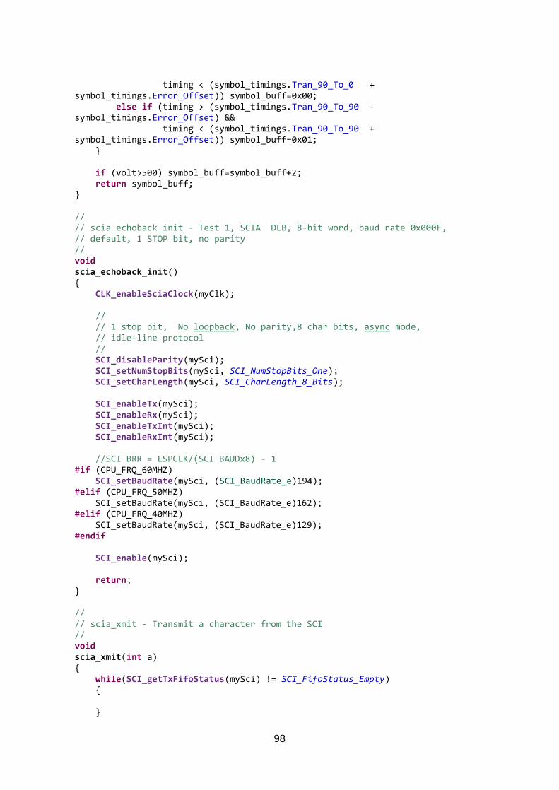
98
timing < (symbol_timings.Tran_90_To_0 + symbol_timings.Error_Offset)) symbol_buff=0x00; else if (timing > (symbol_timings.Tran_90_To_90 - symbol_timings.Error_Offset) && timing < (symbol_timings.Tran_90_To_90 + symbol_timings.Error_Offset)) symbol_buff=0x01; if (volt>500) symbol_buff=symbol_buff+2; return symbol_buff; // // scia_echoback_init - Test 1, SCIA DLB, 8-bit word, baud rate 0x000F, // default, 1 STOP bit, no parity // void scia_echoback_init() CLK_enableSciaClock(myClk); // // 1 stop bit, No loopback, No parity,8 char bits, async mode, // idle-line protocol // SCI_disableParity(mySci); SCI_setNumStopBits(mySci, SCI_NumStopBits_One); SCI_setCharLength(mySci, SCI_CharLength_8_Bits); SCI_enableTx(mySci); SCI_enableRx(mySci); SCI_enableTxInt(mySci); SCI_enableRxInt(mySci); //SCI BRR = LSPCLK/(SCI BAUDx8) - 1 #if (CPU_FRQ_60MHZ) SCI_setBaudRate(mySci, (SCI_BaudRate_e)194); #elif (CPU_FRQ_50MHZ) SCI_setBaudRate(mySci, (SCI_BaudRate_e)162); #elif (CPU_FRQ_40MHZ) SCI_setBaudRate(mySci, (SCI_BaudRate_e)129); #endif SCI_enable(mySci); return; // // scia_xmit - Transmit a character from the SCI // void scia_xmit(int a) while(SCI_getTxFifoStatus(mySci) != SCI_FifoStatus_Empty)

99
SCI_putDataBlocking(mySci, a); // // scia_msg - // void scia_msg(char * msg) int i; i = 0; while(msg[i] != '\0') scia_xmit(msg[i]); i++; // // scia_fifo_init - Initialize the SCI FIFO // void scia_fifo_init() SCI_enableFifoEnh(mySci); SCI_resetTxFifo(mySci); SCI_clearTxFifoInt(mySci); SCI_resetChannels(mySci); SCI_setTxFifoIntLevel(mySci, SCI_FifoLevel_Empty); SCI_resetRxFifo(mySci); SCI_clearRxFifoInt(mySci); SCI_setRxFifoIntLevel(mySci, SCI_FifoLevel_4_Words); return; void Adc_Config() // // Initialize the ADC // ADC_enableBandGap(myAdc); ADC_enableRefBuffers(myAdc); ADC_powerUp(myAdc); ADC_enable(myAdc); ADC_setVoltRefSrc(myAdc, ADC_VoltageRefSrc_Int); // // Enable ADCINT1 in PIE // PIE_enableAdcInt(myPie, ADC_IntNumber_1); // // ADCINT1 trips after AdcResults latch // ADC_setIntPulseGenMode(myAdc, ADC_IntPulseGenMode_Prior);

100
ADC_enableInt(myAdc, ADC_IntNumber_1); // Enabled ADCINT1 // // Disable ADCINT1 Continuous mode // ADC_setIntMode(myAdc, ADC_IntNumber_1, ADC_IntMode_ClearFlag); // // setup EOC2 to trigger ADCINT1 to fire // ADC_setIntSrc(myAdc, ADC_IntNumber_1, ADC_IntSrc_EOC1); // // set SOC0 channel select to ADCINA4 // ADC_setSocChanNumber (myAdc, ADC_SocNumber_1, ADC_SocChanNumber_A2); // // set SOC0 S/H Window to 14 ADC Clock Cycles, (13 ACQPS plus 1) // ADC_setSocSampleWindow(myAdc, ADC_SocNumber_1, ADC_SocSampleWindow_64_cycles); ADC_setSocTrigSrc(myAdc, ADC_SocNumber_1, ADC_SocTrigSrc_Sw); // // ecap1_isr - // __interrupt void ecap1_isr(void) //Clear interrupts for let CEVT1 reset de timestamptimer CAP_clearInt(myCap, CAP_Int_Type_CEVT2); CAP_clearInt(myCap, CAP_Int_Type_Global); // // Acknowledge this interrupt to receive more interrupts from group 4 // PIE_clearInt(myPie, PIE_GroupNumber_4); // // get capture regisers values // count_buff=CAP_getCap2(myCap); uint32_t stop_time = CAP_getCap1(myCap); // // compare capture 1 register, which contains // high level signal time, with stop time // if(stop_time > symbol_timings.Stop_Bit_Time && count_buff > (400) && frame_init==0)

101
frame_init=1; // set new symbol flag new_symbol=1; ADC_forceConversion(myAdc, ADC_SocNumber_1); CAP_rearm(myCap); // // End of File
//
C. TMS320F28027 eCAP module
The enhanced capture (eCAP) module is used in systems where accurate timing of
external events is important.
The so-called eCAP module features the following characteristics:
• Dedicated input capture pin.
• 32-bit time base (counter).
• 4 x 32-bit time-stamp capture registers (CAP1-CAP4).
• 4-stage sequencer (Modulo4 counter) that is synchronized to external
events, ECAP pin rising/falling edges.
• Independent edge polarity (rising/falling edge) selection for all 4 events.
• Input capture signal prescaling (from 2-62)
• One-shot compare register (2 bits) to freeze captures after 1 to 4 time-
stamp events.
• Control for continuous time-stamp captures using a 4-deep circular buffer
(CAP1-CAP4) scheme.
• Interrupt capabilities on any of the 4 capture events.
Figure 76 shows used configuration operation for capture zero-crossing detection
pulses in the receiver, called “Time difference (delta) operation Rising and falling
edge trigger”.

102
Figure 76 Capture sequence for Delta Mode Time-Stamp With Rising and Falling Edge Detect.

103
Glossary
AC Alternating Current
ACK Acknowledgement Packet
AGC Automatic Gain Control
BPSK Binary Phase Shift Keying
CPU Central Processing Unit
CRC Cyclic Redundancy Check
CSMA Carrier Sense Multiple Access
DAC Digital to Analog Converter
DC Direct Current
ESR Equivalent Series Resistance
EVM Evaluation Module
FEC Forward Error Correction
FER Frame Error Rate
FFT Fast Fourier Transform
FM Frequency Modulation
FPGA Field Programmable Gate Array
FSK Frequency Shift Keying
FW Firmware
GPIO General Purpose Input Output
GUI Graphical User Interface
IC Integrated Circuit
LED Light Emitting Diode
MAC Media Access Control
MCU Micro Controller Unit
MOSFET Metal Oxide Substrate Field Effect Transistor
NACK Negative Acknowledgement Packet
NFET Negative channel Field Effect Transistor
OFDM Orthogonal Frequency-Division Multiplexing
OOK On-Off Keying
PHY Physical layer
PLC Power Line Communication
PLL Phase Locked-Loop
PWM Pulse Width Modulation

104
QAM Quadrature Amplitude Modulation
QPSK Quadrature Phase Shift Keying
RGB Red Green Blue
RISC Reduced Instruction Set Computer
SMD Surface Mount Device
SoC System On Chip
UART Universal Asynchronous Receiver-Transmitter
VCO Voltage Controlled Oscillator
VGA Variable Gain Amplifier
VLC Visible Light Communication


![Indoor MIMO Visible Light Communications: Novel Angle ... MIMO Visible Light... · technology [6]. Besides, VLC uses the visible light spectrum which is unregulated and license-free](https://img.pdfslide.net/doc/110x75/5fd68c11806b8407245ac1b8/indoor-mimo-visible-light-communications-novel-angle-mimo-visible-light.jpg)