Embed Size (px)
DESCRIPTION
lll
Citation preview
COMPUTATIONAL GEOMETRIC MECHANICS AND CONTROLOF RIGID BODIES
by
Taeyoung Lee
A dissertation submitted in partial fulfillmentof the requirements for the degree of
Doctor of Philosophy(Aerospace Engineering)
in The University of Michigan2008
Doctoral Committee:
Professor N. Harris McClamroch, Co-ChairAssistant Professor Melvin Leok, Purdue University, Co-ChairProfessor Anthony M. BlochProfessor Jessy W. GrizzleProfessor Daniel J. Scheeres, University of Colorado

c© Taeyoung Lee
2008

ACKNOWLEDGEMENTS
It has been a blessing to me that I could do what I really like to do under encouragements and
supports from my family and friends. As everybody says, a graduation implies a new challenge,
which makes me excited and thrilled. But, before setting out on my new journey of academia, I
would like to express my gratitude to who have influenced on me.
From the very beginning, my parents have inspired me with courage: when I made any decision,
they always supported me and deduced several reasons that made the decision more appropriate.
Now, I understand a little bit about raising a child with absolute trust, instead of having expectations
or concerning about him. It is easy to tell an instructive story to a child, but it requires a tremendous
effort to teach a child by showing a real model of what he ought to be. My parents have been doing
it for me ever since I was born, and I am really proud of my parents.
I have had another exclusive privilege of being advised by Professor N. Harris McClamroch and
Professor Melvin Leok. It has been an honor to have an academic guidance, instruction, encourage-
ment, and insight from both of them, throughout my doctoral study. I am aware that, in some cases,
the relationship between an advisor and a graduate student is similar to that of an employer and an
employee. My relationship with them can be described as the exact opposite: they have treated me
with respect, as an old colleague rather than a student, and they always let me make an important
academic decision by myself. In addition to the technical materials required for this dissertation,
more importantly, I have learned what I can do after my graduation and how I should live my life
as a researcher while enjoying it. Their support and friendship, which also have been from Ms.
Margaret McClamroch, are gratefully acknowledged.
I would like to thank Professor Youdan Kim, whose enthusiasm for control systems engineering
has motivated me from my undergraduate studies. I decided to study aerospace engineering by
myself, but I chose control systems engineering due to his academic excellence and goodness. I
also thank my dissertation committee members, Professor Scheeres, Professor Bloch, and Professor
Grizzle for providing valuable suggestions to improve the quality of my dissertation.
I was also lucky to have been interacting with Eugene Fahnestock, whose sincerity and continu-
ous effort have stimulated my research. It has been a great pleasure to be with the ksag.ae members
and families. In particular, I would like to thank Dr. Chandeok Park, Dr. Kyungjin Lee and Haewon
Lee for their valuable suggestions and for all of the memorable time that we spent together.
Without the constant support of my wife, Heylim, I could not have written a single page of this
dissertation. Being a wife of an international student implies a sacrifice that any other people cannot
fully understand. I am also deeply indebted to her parents. Her contribution to this dissertation
cannot be compared with any others, and this dissertation is gratefully dedicated to her. I would like
to thank Heylim for being with me, and I would like to say to her, “I love you, and I will always.”
ii

TABLE OF CONTENTS
ACKNOWLEDGEMENTS . . . . . . . . . . . . . . . . . . . . . . . . . . . . . . . . ii
LIST OF FIGURES . . . . . . . . . . . . . . . . . . . . . . . . . . . . . . . . . . . . vi
ABSTRACT . . . . . . . . . . . . . . . . . . . . . . . . . . . . . . . . . . . . . . . . . viii
CHAPTER
1. INTRODUCTION . . . . . . . . . . . . . . . . . . . . . . . . . . . . . . . . . . 11.1 Motivation and Goal . . . . . . . . . . . . . . . . . . . . . . . . . . . . . 1
1.1.1 Fundamental Geometric Properties of Rigid Body Dynamics . . 11.1.2 Computational Geometric Mechanics and Control . . . . . . . . 2
1.2 Literature Review . . . . . . . . . . . . . . . . . . . . . . . . . . . . . . 31.2.1 Geometric Numerical Integration . . . . . . . . . . . . . . . . 31.2.2 Geometric Optimal Control . . . . . . . . . . . . . . . . . . . 4
1.3 Outline of Dissertation . . . . . . . . . . . . . . . . . . . . . . . . . . . . 51.4 Contributions . . . . . . . . . . . . . . . . . . . . . . . . . . . . . . . . 7
1.4.1 Summary of Contributions . . . . . . . . . . . . . . . . . . . . 71.4.2 Publications . . . . . . . . . . . . . . . . . . . . . . . . . . . . 9
2. GEOMETRIC MECHANICS FOR RIGID BODIES ON A LIE GROUP . . . 112.1 Lagrangian Mechanics on a Lie Group . . . . . . . . . . . . . . . . . . . 12
2.1.1 Preliminaries on a Lie Group . . . . . . . . . . . . . . . . . . . 122.1.2 Euler-Lagrange Equations . . . . . . . . . . . . . . . . . . . . 132.1.3 Legendre Transformation . . . . . . . . . . . . . . . . . . . . . 162.1.4 Properties of the Lagrangian Flow . . . . . . . . . . . . . . . . 172.1.5 Reduction and Reconstruction . . . . . . . . . . . . . . . . . . 19
2.2 Lagrangian Mechanics on Two-Spheres . . . . . . . . . . . . . . . . . . . 192.2.1 Euler-Lagrange equations . . . . . . . . . . . . . . . . . . . . 202.2.2 Legendre Transformation . . . . . . . . . . . . . . . . . . . . . 24
2.3 Examples of Mechanical Systems on a Lie Group . . . . . . . . . . . . . 262.3.1 Planar Pendulum . . . . . . . . . . . . . . . . . . . . . . . . . 262.3.2 3D Pendulum . . . . . . . . . . . . . . . . . . . . . . . . . . . 272.3.3 3D Pendulum with an Internal Degree of Freedom . . . . . . . 332.3.4 3D Pendulum on a Cart . . . . . . . . . . . . . . . . . . . . . . 362.3.5 Single Rigid Body . . . . . . . . . . . . . . . . . . . . . . . . 382.3.6 Full Body Problem . . . . . . . . . . . . . . . . . . . . . . . . 402.3.7 Two Rigid Bodies Connected by a Ball Joint . . . . . . . . . . 42
2.4 Examples of Mechanical Systems on Two-Spheres . . . . . . . . . . . . . 442.4.1 Double Spherical Pendulum . . . . . . . . . . . . . . . . . . . 442.4.2 n-body Problem on a Sphere . . . . . . . . . . . . . . . . . . . 452.4.3 Interconnection of Spherical Pendula . . . . . . . . . . . . . . 46
iii

2.4.4 Pure Bending of an Elastic Rod . . . . . . . . . . . . . . . . . 462.4.5 Spatial Array of Magnetic Dipoles . . . . . . . . . . . . . . . . 482.4.6 Molecular Dynamics on a Sphere . . . . . . . . . . . . . . . . 49
2.5 Conclusions . . . . . . . . . . . . . . . . . . . . . . . . . . . . . . . . . 503. COMPUTATIONAL GEOMETRIC MECHANICS FOR RIGID BODIES ON
A LIE GROUP . . . . . . . . . . . . . . . . . . . . . . . . . . . . . . . . . . . 513.1 Lie Group Variational Integrator . . . . . . . . . . . . . . . . . . . . . . 52
3.1.1 Discrete-time Euler-Lagrange Equations . . . . . . . . . . . . . 533.1.2 Discrete Legendre Transformation . . . . . . . . . . . . . . . . 563.1.3 Properties of the Discrete-time Lagrangian Flow . . . . . . . . 573.1.4 Discrete Reduction and Reconstruction . . . . . . . . . . . . . 59
3.2 Lie Homogeneous Variational Integrator on Two-Spheres . . . . . . . . . 603.2.1 Discrete-time Euler-Lagrange Equations . . . . . . . . . . . . . 603.2.2 Discrete Legendre Transformation . . . . . . . . . . . . . . . . 63
3.3 Examples of Mechanical Systems on a Lie Group . . . . . . . . . . . . . 673.3.1 Planar Pendulum . . . . . . . . . . . . . . . . . . . . . . . . . 673.3.2 3D Pendulum . . . . . . . . . . . . . . . . . . . . . . . . . . . 693.3.3 3D Pendulum with an Internal Degree of Freedom . . . . . . . 763.3.4 3D Pendulum on a Cart . . . . . . . . . . . . . . . . . . . . . . 793.3.5 Single Rigid Body . . . . . . . . . . . . . . . . . . . . . . . . 843.3.6 Full Body Problem . . . . . . . . . . . . . . . . . . . . . . . . 883.3.7 Two Rigid Bodies Connected by a Ball Joint . . . . . . . . . . 923.3.8 Computational Approach . . . . . . . . . . . . . . . . . . . . . 963.3.9 Summary of Computational Properties . . . . . . . . . . . . . . 99
3.4 Examples of Mechanical Systems on Two-Spheres . . . . . . . . . . . . . 1013.4.1 Double Spherical Pendulum . . . . . . . . . . . . . . . . . . . 1013.4.2 n-body Problem on a Sphere . . . . . . . . . . . . . . . . . . . 1023.4.3 Interconnection of Spherical Pendula . . . . . . . . . . . . . . 1043.4.4 Pure Bending of Elastic Rod . . . . . . . . . . . . . . . . . . . 1053.4.5 Spatial Array of Magnetic Dipoles . . . . . . . . . . . . . . . . 1063.4.6 Molecular Dynamics on a Sphere . . . . . . . . . . . . . . . . 1073.4.7 Computational Approach . . . . . . . . . . . . . . . . . . . . . 1083.4.8 Summary of Computational Properties . . . . . . . . . . . . . . 110
3.5 Conclusions . . . . . . . . . . . . . . . . . . . . . . . . . . . . . . . . . 1114. GEOMETRIC OPTIMAL CONTROL OF RIGID BODIES ON A LIE GROUP112
4.1 Geometric Optimal Control on a Lie Group . . . . . . . . . . . . . . . . . 1124.1.1 Forced Euler-Lagrange Equations on a Lie Group . . . . . . . . 1134.1.2 Optimal Control Problem Formulation . . . . . . . . . . . . . . 1154.1.3 Necessary Conditions for Optimality . . . . . . . . . . . . . . . 115
4.2 Examples of Optimal Control of Rigid Bodies . . . . . . . . . . . . . . . 1194.2.1 Fuel Optimal Attitude Control of a Spacecraft on a Circular Orbit 1194.2.2 Time Optimal Attitude Control of a Free Rigid Body . . . . . . 1224.2.3 Fuel Optimal Attitude Control of a 3D Pendulum with Symmetry 1244.2.4 Fuel Optimal Control of a Rigid Body . . . . . . . . . . . . . . 127
4.3 Conclusions . . . . . . . . . . . . . . . . . . . . . . . . . . . . . . . . . 1295. COMPUTATIONAL GEOMETRIC OPTIMAL CONTROL OF RIGID BOD-
IES ON A LIE GROUP . . . . . . . . . . . . . . . . . . . . . . . . . . . . . . . 1305.1 Computational Geometric Optimal Control on a Lie Group . . . . . . . . 131
iv

5.1.1 Lie Group Variational Integrator with Generalized Forces . . . . 1325.1.2 Discrete-time Optimal Control Problem Formulation . . . . . . 1345.1.3 Discrete-time Necessary Conditions for Optimality . . . . . . . 1345.1.4 Computational Approach for Discrete-time Necessary Conditions 1385.1.5 Direct Optimal Control Approach . . . . . . . . . . . . . . . . 139
5.2 Examples of Optimal Control of Rigid Bodies . . . . . . . . . . . . . . . 1415.2.1 Fuel Optimal Attitude Control of a Spacecraft on a Circular Orbit 1415.2.2 Time Optimal Attitude Control of a Free Rigid Body . . . . . . 1465.2.3 Fuel Optimal Attitude Control of a 3D Pendulum with Symmetry 1505.2.4 Fuel Optimal Control of a Rigid Body . . . . . . . . . . . . . . 1585.2.5 Combinatorial Optimal Control of Spacecraft Formation Recon-
figuration . . . . . . . . . . . . . . . . . . . . . . . . . . . . . 1615.2.6 Fuel Optimal Control of a 3D Pendulum on a Cart . . . . . . . 1685.2.7 Fuel Optimal Control of Two Rigid Bodies Connected by a Ball
Joint with Symmetry . . . . . . . . . . . . . . . . . . . . . . . 1735.3 Conclusions . . . . . . . . . . . . . . . . . . . . . . . . . . . . . . . . . 178
6. CONCLUSIONS . . . . . . . . . . . . . . . . . . . . . . . . . . . . . . . . . . 1796.1 Conclusions . . . . . . . . . . . . . . . . . . . . . . . . . . . . . . . . . 1796.2 Future Work . . . . . . . . . . . . . . . . . . . . . . . . . . . . . . . . . 180
APPENDIX . . . . . . . . . . . . . . . . . . . . . . . . . . . . . . . . . . . . . . . . . 183
BIBLIOGRAPHY . . . . . . . . . . . . . . . . . . . . . . . . . . . . . . . . . . . . . 199
v

LIST OF FIGURES
1.1 Outline of dissertation . . . . . . . . . . . . . . . . . . . . . . . . . . . . . . . . 6
2.1 Procedures to derive Euler-Lagrange equations . . . . . . . . . . . . . . . . . . . 132.2 3D Pendulum . . . . . . . . . . . . . . . . . . . . . . . . . . . . . . . . . . . . 282.3 3D Pendulum with an internal degree of freedom . . . . . . . . . . . . . . . . . . 342.4 3D Pendulum on a cart . . . . . . . . . . . . . . . . . . . . . . . . . . . . . . . 362.5 Two rigid bodies connected by a ball joint . . . . . . . . . . . . . . . . . . . . . 432.6 Examples of mechanical systems on two-spheres . . . . . . . . . . . . . . . . . . 47
3.1 Procedures to derive the continuous/discrete Euler-Lagrange equations . . . . . . 533.2 Numerical simulation for a planar pendulum . . . . . . . . . . . . . . . . . . . . 693.3 Numerical simulation for a 3D pendulum . . . . . . . . . . . . . . . . . . . . . . 753.4 Numerical simulation for a 3D pendulum with an internal degree of freedom . . . 793.5 Numerical simulation for a 3D pendulum on a cart . . . . . . . . . . . . . . . . . 833.6 Numerical simulation for a single rigid body . . . . . . . . . . . . . . . . . . . . 873.7 Numerical simulation for a full two body problem . . . . . . . . . . . . . . . . . 913.8 Numerical simulation for two rigid bodies connect by a ball joint . . . . . . . . . 953.9 Numerical simulation for a double spherical pendulum . . . . . . . . . . . . . . . 1023.10 Numerical simulation for a 3-body problem on sphere . . . . . . . . . . . . . . . 1033.11 Numerical simulation for an interconnection of 4 spherical pendula . . . . . . . . 1043.12 Numerical simulation for an elastic rod . . . . . . . . . . . . . . . . . . . . . . . 1053.13 Numerical simulation for an array of magnetic dipoles . . . . . . . . . . . . . . . 1073.14 Numerical simulation for molecular dynamics on a sphere . . . . . . . . . . . . . 1083.15 Numerical simulation for molecular dynamics on a sphere: kinetic energy distri-
butions over time . . . . . . . . . . . . . . . . . . . . . . . . . . . . . . . . . . 108
4.1 Spacecraft on a circular orbit . . . . . . . . . . . . . . . . . . . . . . . . . . . . 119
5.1 Optimal attitude control of a spacecraft: case 1 . . . . . . . . . . . . . . . . . . . 1455.2 Optimal attitude control of a spacecraft: case 2 . . . . . . . . . . . . . . . . . . . 1455.3 Time optimal attitude control of a free rigid body . . . . . . . . . . . . . . . . . . 1495.4 Two types of the 3D pendulum body . . . . . . . . . . . . . . . . . . . . . . . . 1545.5 Optimal control of a 3D pendulum: case 1 . . . . . . . . . . . . . . . . . . . . . 1565.6 Optimal control of a 3D pendulum: case 2 . . . . . . . . . . . . . . . . . . . . . 1575.7 Optimal orbit transfer of a dumbbell spacecraft: case 1 . . . . . . . . . . . . . . . 1605.8 Optimal orbit transfer of a dumbbell spacecraft: case 2 . . . . . . . . . . . . . . . 1605.9 The initial formation and the desired terminal formation of spacecraft . . . . . . . 1665.10 Optimal spacecraft formation reconfiguration maneuver . . . . . . . . . . . . . . 1675.11 Distribution of the total costs before and after optimization . . . . . . . . . . . . 1675.12 Optimal control of a 3D pendulum on a cart: case 1 . . . . . . . . . . . . . . . . 1715.13 Optimal control of a 3D pendulum on a cart: case 2 . . . . . . . . . . . . . . . . 172
vi

5.14 Falling cat problem . . . . . . . . . . . . . . . . . . . . . . . . . . . . . . . . . 1735.15 Optimal control of two connected rigid bodies: case 1 . . . . . . . . . . . . . . . 1765.16 Optimal control of two connected rigid bodies: case 2 . . . . . . . . . . . . . . . 177
vii

ABSTRACT
COMPUTATIONAL GEOMETRIC MECHANICS AND CONTROLOF RIGID BODIES
by
Taeyoung Lee
This dissertation studies the dynamics and optimal control of rigid bodies from two complemen-
tary perspectives, by providing theoretical analyses that respect the fundamental geometric charac-
teristics of rigid body dynamics and by developing computational algorithms that preserve those
geometric features. This dissertation is focused on developing analytical theory and computational
algorithms that are intrinsic and applicable to a wide class of multibody systems.
A geometric numerical integrator, referred to as a Lie group variational integrator, is devel-
oped for rigid body dynamics. Discrete-time Lagrangian and Hamiltonian mechanics and Lie group
methods are unified to obtain a systematic method for constructing numerical integrators that pre-
serve the geometric properties of the dynamics as well as the structure of a Lie group. It is shown
that Lie group variational integrators have substantial computational advantages over integrators
that preserve either one of none of these properties. This approach is also extended to mechanical
systems evolving on the product of two-spheres.
A computational geometric approach is developed for optimal control of rigid bodies on a Lie
group. An optimal control problem is discretized at the problem formulation stage by using a
Lie group variational integrator, and discrete-time necessary conditions for optimality are derived
using the calculus of variations. The discrete-time necessary conditions inherit the desirable com-
putational properties of the Lie group variational integrator, as they are derived from a symplectic
discrete flow. They do not exhibit the numerical dissipation introduced by conventional numerical
integration schemes, and consequently, we can efficiently obtain optimal controls that respect the
geometric features of the optimality conditions.
The approach that combines computational geometric mechanics and optimal control is illus-
trated by various examples of rigid body dynamics, which include a rigid body pendulum on a
cart, pure bending of an elastic rod, and two rigid bodies connected by a ball joint. Since all of
the analytical and computational results developed in this dissertation are coordinate-free, they are
independent of a specific choice of local coordinates, and they completely avoid any singularity,
ambiguity, and complexity associated with local coordinates. This provides insight into the global
dynamics of rigid bodies.
viii

CHAPTER 1
INTRODUCTION
1.1 Motivation and Goal
This dissertation studies dynamics and optimal control problems for rigid bodies from two com-
plementary perspectives, by providing theoretical analyses that respect the fundamental geometric
characteristics of rigid body dynamics and by developing computational algorithms that preserve
those geometric characteristics.
In control systems engineering, the underlying geometric features of a dynamic system are often
not considered carefully. For example, many control systems are developed for the standard form
of ordinary differential equations, namely x = f(x, u), where the state and the control input are
denoted by x and u, respectively (see, for example, Khalil 2002; Nijmeijer and van der Schaft 1990).
It is assumed that the state and the control input lie in Euclidean spaces, and the system equations
are defined in terms of smooth functions between Euclidean spaces. However, for many interesting
mechanical systems, the configuration space cannot be expressed globally as a Euclidean space. In
addition, general purpose numerical algorithms may not accurately respect fundamental geometric
properties (see Hairer et al. 2000; Leimkuhler and Reich 2004).
In this dissertation, dynamics and optimal control problems for rigid bodies are studied, in-
corporating careful consideration of their geometric features. We explicitly consider the following
research questions: what are the geometric properties of dynamics of rigid bodies, how should
the configuration of rigid bodies be described, how are the geometric properties utilized in control
system analysis and design, and how can the geometric characteristics be preserved in numerical
computations. The goal of this dissertation is to develop both analytical tools and computational
algorithms for rigid body dynamics and control that respect the fundamental geometric features.
1.1.1 Fundamental Geometric Properties of Rigid Body Dynamics
Lie Group Configuration Manifold. The configuration of a rigid body can be described by the
location of its mass center and the orientation of the rigid body in a three-dimensional space. The
location of the rigid body can be expressed in Euclidean space, but the attitude evolves in a nonlinear
space that has a certain geometry.
More precisely, the attitude of a rigid body is defined as the direction of a body-fixed frame
with respect to a reference frame, considered as a linear transformation on the vector space R3;
the attitude can be represented mathematically by a 3 × 3 orthonormal matrix. We require that its
1

determinant is positive in order to preserve the ordering of the orthonormal axes according to the
right-hand rule. The set of 3 × 3 orthonormal matrices with positive determinant is a manifold as
it is locally diffeomorphic to a Euclidean space, and it also has a group structure with the group
action of matrix multiplication. A smooth manifold with a group structure is referred to as a Lie
group; the Lie group of 3 × 3 orthonormal matrices with positive determinant is referred to as the
special orthogonal group, SO(3) (see, for example, Murray et al. 1993; Varadarajan 1984). The
configuration manifold for the combined translational and rotational motion of a rigid body is the
special Euclidean group SE(3), which is a semidirect product SE(3) = SO(3) s©R3. A direct
product of the Lie groups SE(3), SO(3), and Rn can represent the configuration of multiple rigid
bodies, and it is also a Lie group since a product of Lie groups is also a Lie group. Therefore, the
configuration manifold of an interconnection of rigid bodies is also a Lie group.
Lagrangian/Hamiltonian System. Mechanics studies the dynamics of physical bodies acting un-
der forces and potential fields (see Arnold 1989; Goldstein et al. 2001; Meirovitch 2004). In La-
grangian mechanics, the trajectories are obtained by finding the paths that minimize the integral of a
Lagrangian over time, called the action integral. In classical problems, the Lagrangian is chosen as
the difference between kinetic energy and potential energy. The Legendre transformation provides
an alternative description, referred to as Hamiltonian mechanics.
Rigid body dynamics are characterized by Lagrangian/Hamiltonian dynamics. The dynamics of
a Lagrangian or Hamiltonian system has unique geometric properties; the Hamiltonian flow is sym-
plectic, the total energy is conserved in the absence of non-conservative forces, and the momentum
map associated with a symmetry of the system is preserved. By quotienting out the symmetry, a
reduced Lagrangian/Hamiltonian system can be developed (see Marsden 1992).
1.1.2 Computational Geometric Mechanics and Control
Geometric mechanics is a modern description of classical mechanics from the perspective of dif-
ferential geometry (see, for example, Abraham and Marsden 1978; Bloch 2003a; Bullo and Lewis
2005; Jurdjevic 1997; Marsden and Ratiu 1999). It explores the geometric structure of a Lagrangian
or Hamiltonian system through the concept of vector fields, symplectic geometry, and symmetry
techniques. Geometric mechanics provides fundamental insights into mechanics and yields use-
ful tools for dynamics and control theory. For example, geometric mechanics led to the energy-
momentum method in Simo et al. (1990), reduction/reconstruction in Marsden et al. (1990, 2000),
and the controlled Lagrangian method in Bloch et al. (2000, 2001).
The goal of computational geometric mechanics is to construct computational algorithms that
preserve the geometric properties (see Leok 2004). It applies the fundamental principles of geo-
metric mechanics to discrete-time mechanical system to construct geometric structure-preserving
numerical schemes. Since the computational algorithms are developed from discrete-time ana-
logues of physical principles, the geometric properties of the dynamics are preserved naturally.
This is in contrast with the perspective that considers a numerical method as an approximation to a
2

continuous-time equation.
In summary, this dissertation is focused on computational geometric mechanics and control of
rigid bodies. We develop computational methods for rigid bodies, that preserve the underlying
Lagrangian/Hamiltonian system structure of rigid body dynamics as well as the Lie group struc-
ture of the configurations. These methods are applied to numerical integration and optimal control
problems. Prior work related to computational geometric mechanics and control of rigid bodies is
summarized below, followed by an outline and the contributions of this dissertation.
1.2 Literature Review
1.2.1 Geometric Numerical Integration
Geometric numerical integration deals with numerical integration methods that preserve geometric
properties of the flow of a differential equation, such as invariants, symplecticity, and the configura-
tion manifold (see Hairer et al. 2000; Leimkuhler and Reich 2004; McLachlan and Quispel 2001).
Numerical methods that conserve energy and momentum for mechanical systems are referred
to as energy-momentum integrators (see LaBudde and Greenspan 1976; Simo et al. 1992). In these
methods, a free parameter is selected to maintain constant angular momentum; energy conservation
is typically enforced by a momentum-preserving projection onto the manifold of constant energy.
Numerical integration methods that preserve the symplecticity of a Hamiltonian system have
been studied in Lasagni (1988); Sanz-Serna (1992, 1988). Qualitative properties of symplectic in-
tegrators are given in Gonzalez and Simo (1996); Gonzalez et al. (1990), and long-time behavior of
symplectic methods is addressed in Benettin and Giorgilli (1994); Hairer (1994); Hairer and Lubich
(2000). Coefficients of certain Runge-Kutta methods can be chosen to satisfy a symplecticity crite-
rion and order conditions to obtain symplectic Runge-Kutta methods. However, it can be difficult
to construct such integrators, and it is not guaranteed that other invariants of the system, such as a
momentum map, are preserved.
Alternatively, variational integrators are constructed by discretizing Hamilton’s principle, rather
than discretizing the continuous Euler-Lagrange equations (see Marsden and West 2001). This
approach provides a systematic method to develop geometric numerical integrators for Lagrangian /
Hamiltonian systems. The resulting integrators have the desirable property that they are symplectic
and momentum preserving, and they exhibit good energy behavior for exponentially long times.
The idea of developing a discrete-time mechanical system that conserves the constants of motion
appears in the work by Greenspan (1981, 1972); LaBudde and Greenspan (1974), and a discrete-
time mechanical system has been developed according to Hamilton’s principle by Moser and Veselov
(1991); Veselov (1988). The variational view of discrete-time mechanics is further developed
by Kane et al. (1999, 2000); Wendlandt and Marsden (1997), and an intrinsic form of discrete-time
variational principles is established by Marsden and West (2001).
Geometric integrators that preserve the manifold or Lie group structure have been studied (see,
3

for example, Budd and Iserles 1999; Hairer and Wanner 1996; Iserles et al. 2000). A natural ap-
proach to the numerical solution of differential equations on a manifold is by projection. In the work
by Dieci et al. (1994), a solution is updated by a one-step integration method and it is projected to
the manifold on which the system evolves at each time step. This projection may destroy desirable
long-time behavior of one-step methods, since the projection typically corrupts the numerical tra-
jectory. Numerical methods based on local coordinates of the manifold often result in unnecessary
singularities (see Potra and Rheinbold 1991). Differential algebraic approaches have been proposed
to solve nonlinear constrained equations at each time step in Hairer and Wanner (1996).
For differential equations that evolve on a Lie group, a group element can be updated by the
corresponding group action so that the group structure is preserved naturally. This is referred to as
a Lie group method (see Iserles et al. 2000). Among the Lie group methods, the Crouch-Grossman
method updates the group elements by multiple evaluations using the exponential map (see Crouch
and Grossman 1993), and the Munthe-Kaas method is based on a differential equation on the Lie
algebra and uses a single evaluation of the exponential map (see Munthe-Kaas 1995). A homoge-
neous manifold is a manifold on which a Lie group acts continuously in a transitive way. Lie group
methods are extended to homogeneous manifolds in Munthe-Kaas and Zanna (1997).
For mechanical systems evolving on a Lie group, a discrete-time Euler-Poincare equation has
been introduced for a left-invariant Lagrangian by Marsden et al. (1999), with application to the free
attitude dynamics of a rigid body. A similar development is presented for the attitude dynamics of
an axially symmetric rigid body acting under a gravitational potential in Bobenko and Suris (1999).
The idea of using the Lie group structure and the exponential map to numerically compute rigid
body dynamics arises in Krysl (2005); Simo et al. (1992). Symplectic integrators with explicit
constraints on the Lie group structure are applied to rigid body dynamics in Leimkuhler and Reich
(2004).
1.2.2 Geometric Optimal Control
Optimal control problems deal with finding trajectories, such that a certain optimality condition is
satisfied under prescribed constraints (see, for example, Bryson and Ho 1975; Kirk 1970; Sussmann
and Willems 1997). This is typically based on Pontryagin’s minimum principle or the calculus of
variations. Geometric optimal control forms a theoretical foundation for extensions of the minimum
principle to optimal control problems defined on arbitrary differentiable manifolds (see Jurdjevic
1997).
A geometric, intrinsic formulation of the minimum principle is presented in a coordinate-free
fashion in Sussmann (1998a,b). A general formulation of optimal control theory for nonholonomic
systems on a Riemannian manifold is presented in Bloch and Crouch (1993, 1998, 1995). This ap-
proach is applied to both kinematic sub-Riemannian optimal control problems and optimal control
problems for mechanical systems by Bloch (2003a,b). A dynamic interpolation problem on a Rie-
mannian manifold is formulated as an optimal control problem in Hussein and Bloch (2004b), and
this approach is extended to an optimal control problem on a Riemannian manifold with a potential
4

in Hussein and Bloch (2004a). An optimal control problem for nonholonomic and under-actuated
mechanical systems is considered in Hussein and Bloch (2006).
Controllability, observability and optimal control problems on a Lie group have been studied
by Brockett (1973, 1972). A simple closed-form analytic solution for an optimal control problem of
right-invariant systems evolving on a matrix Lie group is presented in Baillieul (1978). An optimal
control problem for a generalized rigid body on SO(n) is considered in Bloch and Crouch (1996). A
general theory of optimal control problems is developed in Jurdjevic (1998a,b, 1997) together with
reachability and controllability conditions; these approaches are based on kinematics equations, and
assume that group elements are directly controlled by elements in the Lie algebra. Optimal control
problems for the dynamics of a rigid body with application to dynamic coverage problem are studied
by Hussein (2005); Hussein and Bloch (2005a,b).
Computational geometric optimal control approaches apply optimal control theory to discrete-
time mechanical systems obtained using geometric numerical integrators. A discrete version of the
generalized rigid body equations and their formulation as an optimal control problem are presented
in Bloch et al. (1998, 2002). Discrete-time optimal control problems for the attitude dynamics of
a rigid body on SO(3) are considered in Bloch et al. (2007); Hussein et al. (2006) based on the
variational integrator. A direct optimal control approach is applied to discrete-time mechanical
systems in Junge et al. (2005), referred to as Discrete Mechanics and Optimal Control.
1.3 Outline of Dissertation
In this dissertation, geometric mechanics and optimal control for rigid bodies are studied, emphasiz-
ing computational geometric methods. The outline of the dissertation is summarized by Figure 1.1.
Results on geometric mechanics for rigid bodies on a Lie group are presented in Chapter 2, and
results on geometric optimal control problems are presented in Chapter 4. Chapter 3 and Chapter 5
present computational geometric algorithms for mechanics and optimal control problems; they can
be considered as discrete-time analogues of Chapter 2 and Chapter 4, respectively. In each chapter,
a general theory is developed first for dynamic systems on an arbitrary Lie group; this general theory
is illustrated by several rigid body systems. The content of each chapter is summarized as follows.
Geometric Mechanics of Rigid Bodies on a Lie Group. Euler-Lagrange equations for mechani-
cal systems evolving on an abstract Lie group are developed according to Hamilton’s principle.
The equivalent Hamilton’s equations are presented in Section 2.1. The essential idea is to express
variations of a curve on a Lie group in terms of Lie algebra elements using the exponential map.
Properties of the Euler-Lagrange equations are discussed, and they are applied to several rigid body
systems evolving on a Lie group in Section 2.3. These results are extended to mechanical systems
on a product of two-spheres in Section 2.2; corresponding examples are given in Section 2.4.
Computational Geometric Mechanics of Rigid Bodies on a Lie Group. This chapter is a discrete-
time version of Chapter 2. Discrete-time Euler-Lagrange equations and discrete-time Hamilton’s
5
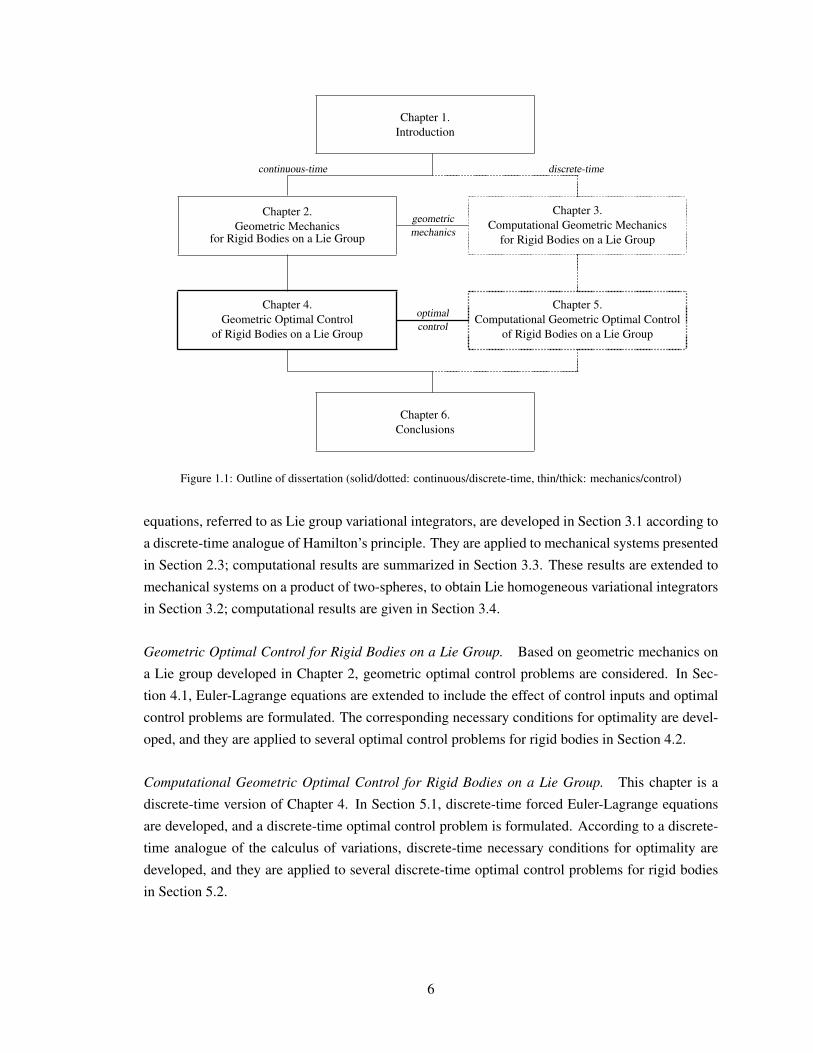
Chapter 1.Introduction
Chapter 2.Geometric Mechanics
for Rigid Bodies on a Lie Group
Chapter 4.Geometric Optimal Control
of Rigid Bodies on a Lie Group
Chapter 3.Computational Geometric Mechanics
for Rigid Bodies on a Lie Group
Chapter 5.Computational Geometric Optimal Control
of Rigid Bodies on a Lie Group
Chapter 6.Conclusions
continuous-time discrete-time
geometricmechanics
optimalcontrol
Figure 1.1: Outline of dissertation (solid/dotted: continuous/discrete-time, thin/thick: mechanics/control)
equations, referred to as Lie group variational integrators, are developed in Section 3.1 according to
a discrete-time analogue of Hamilton’s principle. They are applied to mechanical systems presented
in Section 2.3; computational results are summarized in Section 3.3. These results are extended to
mechanical systems on a product of two-spheres, to obtain Lie homogeneous variational integrators
in Section 3.2; computational results are given in Section 3.4.
Geometric Optimal Control for Rigid Bodies on a Lie Group. Based on geometric mechanics on
a Lie group developed in Chapter 2, geometric optimal control problems are considered. In Sec-
tion 4.1, Euler-Lagrange equations are extended to include the effect of control inputs and optimal
control problems are formulated. The corresponding necessary conditions for optimality are devel-
oped, and they are applied to several optimal control problems for rigid bodies in Section 4.2.
Computational Geometric Optimal Control for Rigid Bodies on a Lie Group. This chapter is a
discrete-time version of Chapter 4. In Section 5.1, discrete-time forced Euler-Lagrange equations
are developed, and a discrete-time optimal control problem is formulated. According to a discrete-
time analogue of the calculus of variations, discrete-time necessary conditions for optimality are
developed, and they are applied to several discrete-time optimal control problems for rigid bodies
in Section 5.2.
6

1.4 Contributions
1.4.1 Summary of Contributions
Coordinate-free approach. One of the common features of the developments in this dissertation
is that the analytical theory and computational methods are developed in terms of a Lie group
representation of the configuration of a rigid body system. Therefore, all of the results presented
in this dissertation are coordinate-free. Representing geometric objects in terms of coordinates can
frequently lead to confusion and complexity, and the corresponding derivations rely on specific
choice of coordinates. This dissertation completely avoids local coordinates, thereby expressing the
results globally in a compact and elegant manner.
For example, consider the attitude dynamics of a single rigid body. The configuration manifold
is SO(3), but there are numerous attitude parameterizations available (see, for example, Shuster
1993; Stuelpnagel 1964). One of the most popular attitude parameterizations is Euler angles. In
addition to the associated singularities, the use of Euler angles can cause confusions since there
are 24 types of Euler angles. The use of Euler angles also leads to complicated trigonometric
expressions. Other minimal attitude representations have similar difficulties.
Non-minimal representations such as quaternions have no coordinate singularities, but they also
introduce certain complications. The group of unit quaternions SU(2) ' S3 double covers SO(3), so
there is an ambiguity in representing the attitude. While the ambiguity of quaternions is the choice
of the sign, there is no consistent way to choose the sign continuously, that is globally valid for
SO(3) (see Marsden and Ratiu 1999). More importantly, the Hamiltonian structure of the attitude
dynamics is complicated when it is expressed in terms of quaternions. For instance, it is difficult to
express the kinetic energy of a rigid body in terms of a quaternion and its time derivative. It is stated
by Leimkuhler and Reich (2004) that although symplectic integration methods based on quaternions
can be formulated, approaches based on the rotation matrix are more efficient and conceptually
easier to implement. For optimal rigid body control problems, the multiplier equations in necessary
conditions for optimality become more complicated if they are written in terms of quaternions (see,
for example, Modgalya and Bhat 2006). Therefore, quaternions result in inherent complications
when applied to dynamics and control problems for rigid bodies. In many engineering applications,
quaternions appear to be simple since they are incorrectly considered to evolve on a flat space,
namely R4, with little attention paid to the unit-length constraint.
In this dissertation, the attitude of a rigid body is represented by a rotation matrix. Geometric
numerical integration algorithms and optimal control approaches are directly developed on SO(3).
The rotation matrix is often avoided, since it is thought that representing a 3-dimensional attitude
using 9 real elements with 6 constraints is inefficient. This redundancy is eliminated by using the
exponential map that allows analysis to be carried out in the Lie algebra that is isomorphic to R3.
For example, necessary conditions for optimality are expressed as compact vector equations on R3;
these equations are more compact than the necessary conditions expressed in terms of quaternions.
They also have the advantage of not having singularity or ambiguity.
7
In summary, this dissertation develops intrinsic, coordinate-free algorithms for computational
geometric mechanics and optimal control problems for rigid bodies. All of the analytical and com-
putational results are independent of a specific choice of local coordinates, and they completely
avoid any singularity, ambiguity, complexity, and confusion associated with local coordinates.
Geometric Numerical Integrators on a Lie Group. The Lie group variational integrators presented
in Chapter 3 are geometric numerical integrators for dynamic systems that evolve on a Lie group,
such as rigid body dynamics. The variational integrators given in Marsden and West (2001) are
geometric integrators that preserve geometric properties of dynamics, but they do not necessarily
conserve the nonlinear structure of the configuration manifold. The Lie group method presented
in Iserles et al. (2000) is for kinematics equations on a Lie group, so it does not guarantee that the
geometric properties of the dynamics are preserved.
This dissertation unifies discrete-time Lagrangian or Hamiltonian mechanics and the Lie group
method. A variational integrator is developed in the context of the Lie group method, so that the
resulting Lie group variational integrator preserves the geometric properties of the dynamics as
well as the structure of the Lie group. For a mechanical system with a Lie group configuration
manifold, such as rigid body dynamics, it is shown that the Lie group variational integrator has
important computational advantages compared to other geometric integrators that preserve either
none or one of these properties (see the numerical example in Section 3.3.6). Due to these superior
computational properties, the Lie group variational integrator has been used to study the dynamics of
the binary near-Earth asteroid 66391 (1999KW4) in joint work between the University of Michigan
and the Jet Propulsion Laboratory, NASA (see Scheeres et al. 2006).
Compared with other geometric integrators for a rigid body, as in the work of Hulbert (1992);
Krysl (2005); Lewis and Simo (1994); Simo and Wong (1991), the Lie group variational integra-
tor provides a systematic method to obtain a class of numerical integrators that preserve all of the
geometric features, rather than developing a specific numerical integrator that preserves only a few
geometric characteristics. Compared with discrete-time mechanics on a Lie group developed by
Bobenko and Suris (1999); Marsden et al. (1999); Moser and Veselov (1991), the Lie group vari-
ational integrator can be applied to a wide class of rigid body dynamics acting under a potential
field.
Optimal Control for Rigid Bodies on a Lie Group. In Chapter 4, optimal control problems for
mechanical systems on a Lie group are formulated, and an intrinsic form of necessary conditions
for optimality are developed. Most existing optimal control theory on a Lie group is established
based on kinematics equations. For example, an optimal attitude control problem of a rigid body is
considered in Jurdjevic (1997) by viewing the angular velocity as a control input. This dissertation
deals with optimal control problems of dynamic systems with a Lie group configuration manifold.
More precisely, it may be considered as an optimal control problem on a tangent bundle of a Lie
group. Compared with the work by Hussein (2005), where optimal control problems on SO(3) and
8

SE(3) are considered, the necessary conditions presented in Section 4.1.3 are applied to a more
general class of dynamic systems on an abstract Lie group.
A direct optimal control approach has been applied to discrete-time mechanical systems ob-
tained by variational integrators in Junge et al. (2005, 2006), where control input parameters are
optimized using a general constrained parameter optimization scheme such as sequential quadratic
programming. The computational geometric optimal control approach presented in Chapter 5 uses
a discrete-time analogue of the calculus of variations to derive an intrinsic form of discrete-time
optimality conditions, and a computational approach to solve the optimality conditions is presented.
Compared with the geometric structure-preserving optimal control approach on SO(3) by Bloch
et al. (2007); Hussein et al. (2006), the discrete-time optimality conditions presented in Section 5.1
can be applied to general optimal control problems on an arbitrary Lie group; they are applied to
nontrivial rigid body optimal control problems in Section 5.2.
Examples of Nontrivial Rigid Body Systems. In this dissertation, the abstract theory for computa-
tional geometric mechanics and optimal control is applied to several nontrivial rigid body systems.
For example, in Section 3.3, Lie group variational integrators are developed for a rigid body pen-
dulum, a pendulum with an internal proof mass, a pendulum on a moving cart, rigid bodies acting
under mutual potential, and connected rigid bodies. Computational results are also presented for
each system. In Section 3.4, several mechanical systems from various scientific fields, such as an
elastic rod, magnetic dipoles, and molecular dynamics, are considered. Computational geomet-
ric optimal control is applied to minimum time, and minimum fuel optimal control problems of a
rigid body, and extended to optimal control problems with symmetry and a combinatorial optimal
formation reconfiguration problem in Section 5.2.
New theoretical results in geometric mechanics and control are developed in an abstract form.
This dissertation also studies numerous nontrivial rigid body systems that have engineering impor-
tance.
1.4.2 Publications
The contributions in this dissertation have been published in the following journals, conference
proceedings, and book chapter. These contributions that are currently under review/revision are
indicated.
Computational Geometric Mechanics
• T. Lee, M. Leok, and N. H. McClamroch. A Lie group variational integrator for the attitude
dynamics of a rigid body with application to the 3D pendulum. In Proceedings of the IEEE
Conference on Control Application, pages 962–967, 2005.
• E. Fahnestock, T. Lee, M. Leok, N. H. McClamroch, and D. Scheeres. Polyhedral potential
and variational integrator computation of the full two body problem. In Proceedings of the
AIAA/AAS Astrodynamics Specialist Conference and Exhibit, 2006.
9

• T. Lee, M. Leok, and N. H. McClamroch. Lie group variational integrators for the full body
problem in orbital mechanics. Celestial Mechanics and Dynamical Astronomy, 98(2):121–
144, June 2007.
• T. Lee, M. Leok, and N. H. McClamroch. Lie group variational integrators for the full body
problem. Computer Methods in Applied Mechanics and Engineering, 196:2907–2924, 2007.
• T. Lee, M. Leok, and N. H. McClamroch. Lagrangian mechanics and variational integrators
on two-spheres. 2007, under revision. URL http://arxiv.org/abs/0707.0022.
Computational Geometric Optimal Control
• T. Lee, M. Leok, and N. H. McClamroch. Attitude maneuvers of a rigid spacecraft in a
circular orbit. In Proceedings of the American Control Conference, pages 1742–1747, 2005.
• T. Lee, M. Leok, and N. H. McClamroch. Optimal control of a rigid body using geometrically
exact computations on SE(3). In Proceedings of the IEEE Conference on Decision and
Control, pages 2170–2175, 2006.
• T. Lee, M. Leok, and N. H. McClamroch. Discrete control systems. Invited article for the
Encyclopedia of Complexity and System Science. Springer, 2007.
• T. Lee, M. Leok, and N. H. McClamroch. Computational geometric optimal control of
rigid bodies. Communications in Information and Systems, special issue dedicated to R. W.
Brockett, 2007. submitted.
• T. Lee, M. Leok, and N. H. McClamroch. Optimal attitude control of a rigid body using
geometrically exact computations on SO(3). Journal of Dynamical and Control Systems,
2007. accepted.
• T. Lee, M. Leok, and N. H. McClamroch. Optimal attitude control for a rigid body with
symmetry. In Proceedings of the American Control Conference, pages 1073–1078, 2007.
• T. Lee, M. Leok, and N. H. McClamroch. A combinatorial optimal control problem for
spacecraft formation reconfiguration. In Proceedings of the IEEE Conference on Decision
and Control, pages 5370–5375, 2007.
• T. Lee, M. Leok, and N. H. McClamroch. Time optimal attitude control for a rigid body. In
Proceedings of the American Control Conference, 2008. accepted.
This research has been recognized by the following awards:
• Rackham International Students Fellowship, University of Michigan 2006
• Rackham Predoctoral Fellowship, University of Michigan 2006-2007
• SIAM Computational Science and Engineering, BGCE Student Paper Prize, finalist 2007
• Distinguished Achievement Award, College of Engineering, University of Michigan 2008
• Ivor K. McIvor Award, College of Engineering, University of Michigan 2008
10

CHAPTER 2
GEOMETRIC MECHANICS FOR RIGID BODIES ON A LIEGROUP
This chapter deals with geometric mechanics for rigid bodies that evolve on a Lie group. The
goal is to develop an intrinsic form of Euler-Lagrange equations on an arbitrary Lie group, and
to show several properties of Lagrangian flows. These are applied to several rigid body systems
evolving on a Lie group, and extended to mechanical systems on a product of two-spheres.
2.1 Lagrangian mechanics on a Lie group
2.1.2 Euler-Lagrange equations
2.1.3 Legendre transformation
2.1.4 Properties of the Lagrangian flow2.1.5 Reduction and reconstruction
2.3 Examples of mechanical systemson a Lie group
2.3.1 Planar pendulum
2.3.2 3D pendulum
2.3.3 3D pendulum with an internal mass
2.3.4 3D pendulum on a cart
2.3.5 Single rigid body
2.3.6 Full body problem
2.3.7 Two rigid bodies connected by a ball joint
2.2 Lagrangian mechanics on two-spheres
2.2.1 Euler-Lagrange equations
2.2.2 Legendre transformation
2.4 Examples of mechanical systemson two-spheres
2.4.1 Double spherical pendulum2.4.2 n-body problem on a sphere2.4.3 Interconnection of spherical pendula2.4.4 Pure bending of elastic rod2.4.5 Spatial array of magnetic dipoles2.4.6 Molecular dynamics
This chapter is organized as follows. In Section 2.1, we develop geometric mechanics on a
Lie group; Euler-Lagrange equations are developed and several properties of Lagrangian flow are
discussed. These results are applied to several rigid body dynamics in Section 2.3. The remaining
part of this chapter develops geometric mechanics on a product of two-spheres. Since the two-
sphere is a homogeneous manifold on which a Lie group acts transitively, the Lagrangian mechanics
on a Lie group developed in Section 2.1 can be easily extended to the two sphere. Euler-Lagrange
equations on a product of two-spheres are developed in Section 2.2, and they are applied to several
11

mechanical systems in Section 2.4.
2.1 Lagrangian Mechanics on a Lie Group
Geometric mechanics is a modern description of classical mechanics from the perspective of dif-
ferential geometry (see, for example, Abraham and Marsden 1978; Bloch 2003a; Bullo and Lewis
2005; Jurdjevic 1997; Marsden and Ratiu 1999). It explores the geometric structure of a Lagrangian
or Hamiltonian system through the concept of vector fields, symplectic geometry, and symmetry
techniques. This section develops Lagrange mechanics on a Lie group; Euler-Lagrange equations
for a mechanical system evolving on an abstract Lie group are derived, and the symplectic property
and symmetry of Lagrangian flow are discussed.
The dynamics of rigid bodies evolve on a Lie group. For example, the configuration manifold for
the attitude dynamics of a rigid body is the special orthogonal group SO(3), and the configuration
manifold for combined translational and rotational motion of a rigid body is the special Euclidean
group SE(3). A direct product of Lie groups SE(3), SO(3), and Rn can represent a configuration
manifold of multiple rigid bodies, which is also a Lie group.
However, much of the literature on dynamics of rigid bodies relies on local coordinates of a
Lie group. For example, a time optimal attitude maneuver of a rigid body is studied in terms
of Euler angles by Bilimoria and Wie (1993), and constrained equations of motion in multibody
dynamics are developed in terms of local coordinates on a manifold by Yen (1993). As discussed
in Section 1.4.1, representing geometric objects in terms of local coordinates frequently leads to
confusion and complexity.
The analytical results of this section are coordinate-free; they are independent of a specific
choice of local coordinates, and they completely avoid any singularity, ambiguity, and confusion
associated with local coordinates. The resulting intrinsic form of the Euler-Lagrange equations are
more compact that equations expressed in terms of local coordinates. Since these are developed for
mechanical systems that evolves on an arbitrary Lie group, they provides a general framework that
can be uniformly applied to dynamics of multiple rigid bodies.
This section is organized as follows. Section 2.1.1 provides preliminaries on a Lie group.
Euler-Lagrange equations and Hamilton’s equations on an arbitrary Lie group are developed in
Section 2.1.2 and in Section 2.1.3, respectively. Properties of Lagrangian flow and Lagrange-Routh
reduction are described in Section 2.1.4 and Section 2.1.5.
2.1.1 Preliminaries on a Lie Group
We first summarize basic definitions and properties of a Lie group (see, for example, Bloch 2003a;
Bullo and Lewis 2005; Marsden and Ratiu 1999; Varadarajan 1984). A Lie group is a differentiable
manifold that has a group structure such that the group operation is a smooth map. A Lie algebra is
the tangent space of the Lie group G at the identity element e ∈ G, with a Lie bracket [·, ·] : g×g→ g
that is bilinear, skew symmetric, and satisfies the Jacobi identity.
12
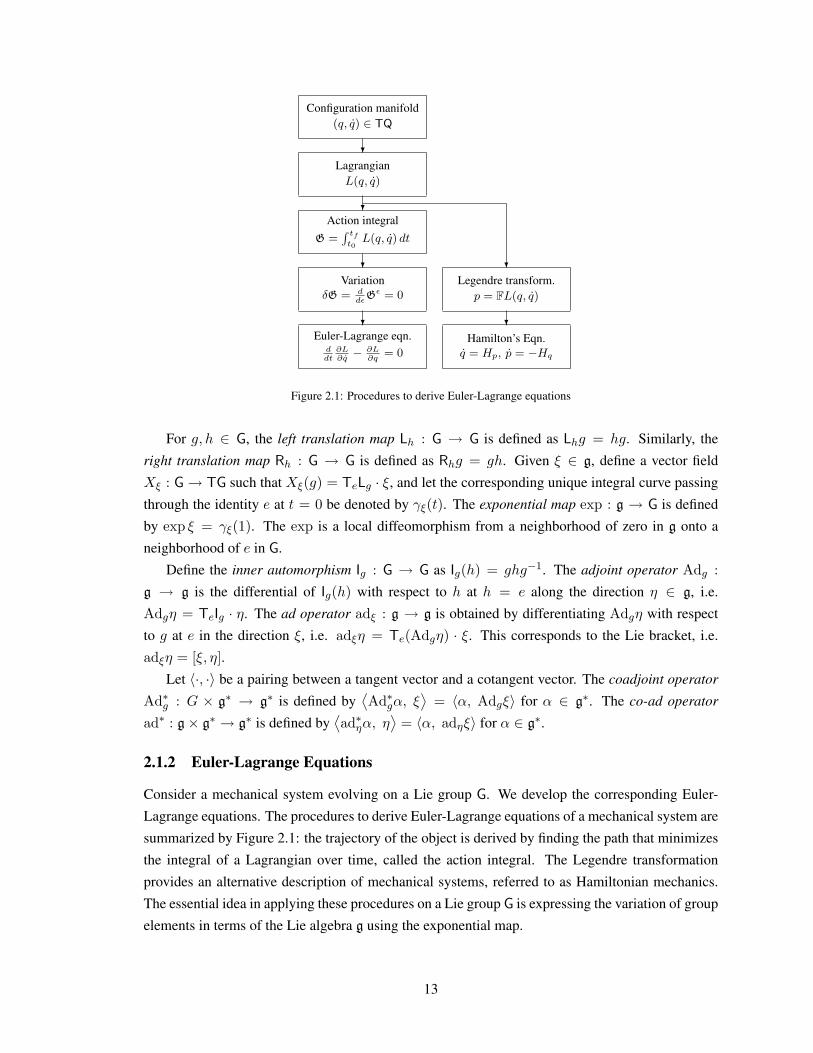
Configuration manifold(q, q) ∈ TQ
?LagrangianL(q, q)
?
?
Action integralG =
∫ tft0L(q, q) dt
?Variation
δG = ddε
Gε = 0
?Euler-Lagrange eqn.ddt∂L∂q− ∂L
∂q= 0
Legendre transform.p = FL(q, q)
?
Hamilton’s Eqn.q = Hp, p = −Hq
Figure 2.1: Procedures to derive Euler-Lagrange equations
For g, h ∈ G, the left translation map Lh : G → G is defined as Lhg = hg. Similarly, the
right translation map Rh : G → G is defined as Rhg = gh. Given ξ ∈ g, define a vector field
Xξ : G→ TG such that Xξ(g) = TeLg · ξ, and let the corresponding unique integral curve passing
through the identity e at t = 0 be denoted by γξ(t). The exponential map exp : g → G is defined
by exp ξ = γξ(1). The exp is a local diffeomorphism from a neighborhood of zero in g onto a
neighborhood of e in G.
Define the inner automorphism Ig : G → G as Ig(h) = ghg−1. The adjoint operator Adg :g → g is the differential of Ig(h) with respect to h at h = e along the direction η ∈ g, i.e.
Adgη = TeIg · η. The ad operator adξ : g → g is obtained by differentiating Adgη with respect
to g at e in the direction ξ, i.e. adξη = Te(Adgη) · ξ. This corresponds to the Lie bracket, i.e.
adξη = [ξ, η].Let 〈·, ·〉 be a pairing between a tangent vector and a cotangent vector. The coadjoint operator
Ad∗g : G × g∗ → g∗ is defined by⟨Ad∗gα, ξ
⟩= 〈α, Adgξ〉 for α ∈ g∗. The co-ad operator
ad∗ : g× g∗ → g∗ is defined by⟨ad∗ηα, η
⟩= 〈α, adηξ〉 for α ∈ g∗.
2.1.2 Euler-Lagrange Equations
Consider a mechanical system evolving on a Lie group G. We develop the corresponding Euler-
Lagrange equations. The procedures to derive Euler-Lagrange equations of a mechanical system are
summarized by Figure 2.1: the trajectory of the object is derived by finding the path that minimizes
the integral of a Lagrangian over time, called the action integral. The Legendre transformation
provides an alternative description of mechanical systems, referred to as Hamiltonian mechanics.
The essential idea in applying these procedures on a Lie group G is expressing the variation of group
elements in terms of the Lie algebra g using the exponential map.
13

Configuration Manifold and Lagrangian
The configuration manifold is a Lie group G. We identify the tangent bundle TG with G× g by left
trivialization. For example, a tangent vector (g, g) ∈ TgG is expressed as
g = TeLg · ξ = gξ (2.1)
for ξ ∈ g. We assume the Lagrangian of the mechanical system is given by L(g, ξ) : G× g→ R.
Action Integral
Define the action integral as
G =∫ tf
t0
L(g, ξ) dt.
Hamilton’s principle states that the variation of the action integral is equal to zero.
δG = δ
∫ tf
t0
L(g, ξ) dt. (2.2)
Variations
Let g(t) be a differential curve in G defined for t ∈ [t0, tf ]. The variation is a differentiable mapping
gε(t) : (−c, c) × [t0, tf ] → G for c > 0 such that g0(t) = g(t) for any t ∈ [t0, tf ], and gε(t0) =g(t0), gε(tf ) = g(tf ) for any ε ∈ (−c, c). We express the variation using the exponential map as
gε(t) = g exp εη(t), (2.3)
for a curve η(t) in g. It is easy to show that (2.3) is well defined for some constant c as the exponen-
tial map is a local diffeomorphism between g and G, and it satisfies the properties of the variation
provided η(t0) = η(tf ) = 0. Since this is obtained by a group operation, it is also guaranteed that
the variation lies on G for any η(t).
The corresponding infinitesimal variation of g is given by
δg(t) =d
dε
∣∣∣∣ε=0
gε(t) = TeLg(t) ·d
dε
∣∣∣∣ε=0
exp εη(t)
= g(t)η(t). (2.4)
For each t ∈ [t0, tf ], the infinitesimal variation δg(t) lies in the tangent space Tg(t)G. Using this
expression and (2.1), the infinitesimal variation of ξ(t) is obtained as follows (see Bloch et al. 1996;
Marsden and Ratiu 1999, and Appendix A.4).
δξ(t) = η(t) + adξ(t)η(t). (2.5)
Equations (2.4) and (2.5) are infinitesimal variations of (g(t), ξ(t)) : [t0, tf ]→ G× g, respectively.
14

Euler-Lagrange Equations
The variation of the Lagrangian can be written as
δL(g, ξ) = DgL(g, ξ) · δg + DξL(g, ξ) · δξ,
where DgL ∈ T∗G denotes the derivative of the Lagrangian L with respect to g, given by
d
dε
∣∣∣∣ε=0
L(gε, ξ) = DgL(g, ξ) · δg,
and DξL(g, ξ) ∈ g∗ is defined similarly. Since T(Lg Lg−1) = TLg TLg−1 is equal to the identity
map on TG, this can be written as
δL(g, ξ) = 〈DgL(g, ξ), δg〉+ 〈DξL(g, ξ), δξ〉
=⟨DgL(g, ξ), (TeLg TgLg−1) · δg
⟩+ 〈DξL(g, ξ), δξ〉 .
Substituting (2.4) and (2.5), we obtain
δL(g, ξ) = 〈DgL(g, ξ), TeLg · η〉+ 〈DξL(g, ξ), η + adξη〉
=⟨T∗eLg ·DgL(g, ξ) + ad∗ξ ·DξL(g, ξ), η
⟩+ 〈DξL(g, ξ), η〉 . (2.6)
Since variation and integration commute, the variation of the action integral is given by
δG =∫ tf
t0
δL(g, ξ) dt.
Substituting (2.6) and using integration by parts, the variation of the action integral is given by
δG =∫ tf
t0
⟨T∗eLg ·DgL(g, ξ) + ad∗ξ ·DξL(g, ξ), η
⟩+ 〈DξL(g, ξ), η〉 dt
= 〈DξL(g, ξ), η〉∣∣∣∣tft0
+∫ tf
t0
⟨T∗eLg ·DgL(g, ξ) + ad∗ξ ·DξL, η
⟩−⟨d
dtDξL(g, ξ), η
⟩dt.
(2.7)
Since η(t) = 0 at t = t0 and t = tf , the first term of the above equation vanishes. Thus, we obtain
δG =∫ tf
t0
⟨T∗eLg ·DgL(g, ξ) + ad∗ξ ·DξL(g, ξ), η
⟩−⟨d
dtDξL(g, ξ), η
⟩dt. (2.8)
From Hamilton’s principle, δG = 0 for all η ∈ g, which yields the Euler-Lagrange equations on G.
Proposition 2.1 Consider a mechanical system evolving on a Lie group G. We identify the tangent
bundle TG with G × g by left trivialization. Suppose that the Lagrangian is defined as L(g, ξ) :
15
G× g→ R. The corresponding Euler-Lagrange equations are given by
d
dtDξL(g, ξ)− ad∗ξ ·DξL(g, ξ)− T∗eLg ·DgL(g, ξ) = 0, (2.9)
g = gξ. (2.10)
Remark 2.1 The essential idea of this development is expressing the variation of a curve in G using
the exponential map, as given by (2.3). The expression for the variation is carefully chosen such that
the varied curve lies on the configuration manifold G. The use of the exponential map exp : g→ G
is desirable in two aspects: (i) since the variation is obtained by a group operation, it is guaranteed
to lie on G, and (ii) the variation is parameterized by a curve in a linear vector space g.
Remark 2.2 If the Lagrangian is not dependent on G, the third term of (2.9) vanishes. The resulting
equation is equivalent to the Euler-Poincare equation, and (2.10) is a reconstruction equation (see
Marsden and Ratiu 1999). Therefore, (2.9) can be considered as a generalization of the Euler-
Poincare equation.
Remark 2.3 These equations are obtained using the left trivialization. Therefore, the velocity ξ
may be considered as a quantity expressed in the body fixed frame. We can develop similar equa-
tions using the right trivialization to obtain the equations of motion expressed in the reference frame.
This is summarized by the following corollary.
Corollary 2.1 Consider a mechanical system evolving on a Lie group G. We identify the tangent
bundle TG with G × g by right trivialization. Suppose that the Lagrangian is defined as L(g, ς) :G× g→ R. The corresponding Euler-Lagrange equations are given by
d
dtDςL(g, ς) + ad∗ς ·DςL(g, ς)− T∗eRg ·DgL(g, ς) = 0, (2.11)
g = ςg. (2.12)
2.1.3 Legendre Transformation
We identify the tangent bundle TG with G× g using the left trivialization. Using this, the cotangent
bundle T∗G can be identified with G × g∗. For the given Lagrangian, the Legendre transformation
FL : G× g→ G× g∗ is defined as
FL(g, ξ) = (g, µ), (2.13)
where µ ∈ g∗ is given by
µ = DξL(g, ξ). (2.14)
If the Legendre transformation is a diffeomorphism, the corresponding Lagrangian is called ahyperregular Lagrangian, which induces a Hamiltonian system on G× g∗.
16

Corollary 2.2 Consider a mechanical system evolving on a Lie group G. We identify the tangent
bundle TG with G × g by left trivialization. Suppose that the Lagrangian given by L(g, ξ) : G ×g → R is hyperregular. Then, the Legendre transformation yields Hamilton’s equations that are
equivalent to the Euler-Lagrange equations presented in Proposition 2.1.
d
dtµ− ad∗ξµ− T∗eLg ·DgL(g, ξ) = 0, (2.15)
g = gξ, (2.16)
where µ = DξL(g, ξ) ∈ g∗.
2.1.4 Properties of the Lagrangian Flow
Here we show two properties of the Lagrangian flow, namely symplecticity and momentum preser-
vation. The subsequent development can be considered as a special form of the general properties
of Lagrangian flows, applied to a Lie group configuration manifold (see Marsden and West 2001).
Symplecticity
Let ΘL be the Lagrangian one-form on G× g given by
ΘL(g, ξ) · (δg, δξ) =⟨DξL(g, ξ), g−1δg
⟩(2.17)
The Lagrangian symplectic two-form ΩL is the exterior derivative of the Lagrangian one-forme, i.e.ΩL = dΘL. We define the Lagrangian flow map FL : (G× g)× [0, tf − t0]→ (G× g) as the flowof (2.9) and (2.10).
Proposition 2.2 The Lagrangian flow preserves the Lagrangian symplectic two-form as follows
(FTL )∗ΩL = ΩL (2.18)
for T = tf − t0.
Proof. Define the solution space CL to be the set of solutions g(t) : [t0, tf ] → G of (2.9) and
(2.10). Since an element of CL is uniquely determined by the initial condition (g(0), ξ(0)) ∈ G×g,
we can identify CL with the space of initial conditions G × g. Define the restricted action map
G : G× g→ R by
G(g0, ξ0) = G(g(t)),
where g(t) ∈ CL with (g(0), g−1(0)g(0)) = (g0, ξ0). Since the curve g(t) satisfies (2.9) and (2.10),
(2.7) reduces to
dG · w = ((FTL )∗ΘL −ΘL) · w (2.19)
17

for any w = (δg0, δξ0) ∈ T(G × g). We take the exterior derivative of (2.19). Since exterior
derivatives and pull back commute, we obtain
d2G = ((FTL )∗dΘL − dΘL).
Since d2G = 0 for any zero-form G, we obtain (2.18).
Noether’s Theorem
Suppose that a Lie group H, with the Lie algebra h, acts on G. A left action of H on G is a smooth
mapping Φ : H× G→ G such that Φ(e, g) = g, and Φ(h,Φ(h′, g)) = Φ(hh′, g) for any g ∈ G and
h, h′ ∈ H. Let Φh : G→ G be defined such that Φh(g) = Φ(h, g).
Let φL : TG → G × g be the left trivialization given by φL(g, g) = (g, g−1g). For ζ ∈ h, the
infinitesimal generators ζG : G → G× g, and ζG×g : G× g → T(G× g) for the action are defined
by
ζG(g) = φL d
dε
∣∣∣∣ε=0
ΦexpH εζ(g), (2.20)
ζG×g(g, ξ) =d
dε
∣∣∣∣ε=0
φL TgΦexpH εζ(g) · (φ−1L (g, ξ)). (2.21)
We define the Lagrangian momentum map JL : G× g→ h∗ to be
JL(g, ξ) · ζ = ΘL · ζG×g(g, ξ). (2.22)
Proposition 2.3 Suppose that the Lagrangian is infinitesimally invariant under the lifted action, i.e.
dL(g, ξ) · ζG×g = 0 for any ζ ∈ h. Then, the Lagrangian flow preserves the momentum map.
JL(FTL (g, ξ)) = JL(g, ξ), (2.23)
This is referred to as Noether’s theorem.
Proof. Since the action is the integral of the Lagrangian, dL(g, ξ) · ζG×g = 0 implies that dG ·ζG×g = 0, where we consider that the group action Φh is applied to each point of a curve. The
invariance of the action integral implies that the action maps a solution curve to another solution
curve. Thus, we can restrict dG · ζG×g = 0 to the solution space to obtain
dG · ζG×g = 0.
But, from (2.19), we have
dG · ζG×g = ((FTL )∗ΘL −ΘL) · ζG×g = 0 (2.24)
18

for any ζ ∈ h. Substituting the definition of the momentum map given by (2.22) into this, we obtain
(2.23).
2.1.5 Reduction and Reconstruction
We have shown that if the Lagrangian is infinitesimally invariant under the lifted action of a Lie
group H on G, the corresponding momentum map is preserved along the Lagrangian flow. Suppose
that the Lie group H acts freely and properly on G, and the Lagrangian is invariant under the action
H. This is referred to as the symmetry of the Lagrangian. Then, the configuration manifold can
be reduced to a quotient space G/H, referred to as the shape space. Because the action is free and
proper, it is guaranteed that the shape space is a smooth manifold.
More precisely, for a given curve g(t) in the solution space CL and the corresponding value of
the momentum map, there exists a unique curve in the shape space G/H satisfying reduced Euler-
Lagrange equations. If the initial condition g(t0) is known, the curve g(t) in G can be reconstructed
from the solution of the reduced Euler-Lagrange equations in the shape space G/H. These are
referred to as reduction and reconstruction for mechanical systems.
The procedure for the Lagrangian-Routh reduction and reconstruction is as follows (see Mars-
den et al. 2000). We define a mechanical connectionA : G×g→ h from the momentum map. This
yields a one-form Aν on G× g paired with the value of the momentum map ν ∈ h∗. The Routhian
Rν : G × g → R is defined by subtracting the one-form Aν from the Lagrangian. The Routhian
satisfies the Lagrange-d’Alembert principle with the magnetic two-form obtained from the exterior
derivative of the one-form Aν . This form of the variational principle and the Routhian reduce onto
the ν-level set of the momentum map, which provides the reduced Euler-Lagrange equations on the
shape space.
For a given solution of the reduced Euler-Lagrange equations, we find the horizontal lift of the
curve on G. Applying the mechanical connection to the time derivatives of the lifted curve provides a
reconstruction equation. A particular example for the Lagrange-Routh reduction and reconstruction
is presented in Appendix A.3.
2.2 Lagrangian Mechanics on Two-Spheres
In the previous section, we have developed Euler-Lagrange equations for mechanical systems evolv-
ing on a Lie group, and the symplectic property and symmetry of the Lagrangian flow are discussed.
The essential idea in developing the Euler-Lagrange equations on a Lie group is to express the vari-
ation of a curve on a Lie group in terms of a curve on the corresponding Lie algebra using the
exponential map.
In this section, we develop Euler-Lagrange equations for mechanical systems evolving on a
product of two-spheres
S2 = q ∈ R3 | q · q = 1.
19

The two-sphere S2 is not a Lie group, but the special orthogonal group SO(3) = R ∈ R3×3 |RTR =I, detR = 1 acts on the two-sphere transitively, i.e. for any q1, q2 ∈ S2, there exists a R ∈ SO(3)such that q2 = Rq1. Therefore, we can express the variation of a curve on S2 in terms of a curve
on so(3) ' R3 using the exponential map of SO(3), from which Euler-Lagrange equations can be
developed.
In most of the literature that treats dynamic systems on (S2)n, either 2n angles or n explicit
equality constraints enforcing unit length are used to describe the configuration of the system (see,
for example, Bendersky and Sandler 2006; Marsden et al. 1993). These descriptions involve compli-
cated trigonometric expressions and introduce additional complexity in analysis and computations.
In this section, we develop Euler-Lagrange equations on (S2)n without need of local parame-
terizations, constraints, or reprojections. This yields a remarkably compact form of the equations
of motion, and also provides insight into the global dynamics on (S2)n. A manifold on which a
Lie group acts in a transitively way is referred to as a homogeneous manifold. The key idea of this
development can be generalized to an abstract homogeneous manifold.
2.2.1 Euler-Lagrange equations
The procedures to derive Euler-Lagrange equations are summarized by Figure 2.1: the trajectory of
the object is derived by finding the path that minimizes the integral of a Lagrangian over time, called
the action integral. The Legendre transformation provides an alternative description of mechanical
systems, referred to as Hamiltonian mechanics. The essential idea is to express the variation of a
curve on S2 in terms of the Lie algebra so(3) using the exponential map.
Configuration Manifold and Lagrangian
The two-sphere is the set of points that have unit length from the origin of R3, i.e. S2 = q ∈R3 | q · q = 1. The tangent space TqS
2 for q ∈ S2 is a plane tangent to the two-sphere at the point
q. Thus, a curve q : R→ S2 and its time derivative satisfy q · q = 0. The time-derivative of a curve
can be written as
q = ω × q, (2.25)
where the angular velocity ω ∈ R3 is constrained to be orthogonal to q, i.e. q · ω = 0. The time
derivative of the angular velocity is also orthogonal to q, i.e. q · ω = 0.
We consider a mechanical system evolving on an n product of two-spheres, S2 × · · · × S2 =(S2)n. We assume that the Lagrangian L : T(S2)n → R is given by the difference between a
quadratic kinetic energy and a configuration-dependent potential energy as follows.
L(q1, . . . , qn, q1, . . . , qn) =12
n∑i,j=1
Mij qi · qj − U(q1, . . . , qn), (2.26)
where (qi, qi) ∈ TS2 for i ∈ 1, . . . , n, and Mij ∈ R is the i, j-th element of a symmetric positive
20
definite inertia matrix M ∈ Rn×n for i, j ∈ 1, . . . , n. The configuration dependent potential is
denoted by U : (S2)n → R. Here, we assume the inertia matrix is constant, but it can be readily
generalized to mechanical systems with a configuration dependent inertia.
Action Integral
Define the action integral as
G =∫ tf
t0
L(q1, . . . , qn, q1, . . . , qn) dt.
Hamilton’s principle states that the variation of the action integral is equal to zero.
Variations
Let qi(t) be a differentiable curve in S2 defined for t ∈ [t0, tf ]. The variation is a differentiable
mapping qεi (t) : (−c, c) × [t0, tf ] → S2 for c > 0 such that q0i (t) = qi(t) for any t ∈ [t0, tf ] and
qεi (t0) = qi(t0), qεi (tf ) = q(tf ) for any ε ∈ (−c, c). Since the special orthogonal group SO(3) acts
on S2 in a transitive way, we can express the variation of qi(t) using the exponential map on SO(3)as follows.
qεi (t) = exp εηi(t) qi(t) (2.27)
for a curve ηi(t) in R3. It is easy to show that (2.27) is well defined since the exponential map is a
local diffeomorphism between so(3) and SO(3), and SO(3) acts on S2. It satisfies other properties
of the variation provided that ηi(t0) = ηi(tf ) = 0. We assume ηi(t) · qi(t) = 0 for t ∈ [t0, tf ].The corresponding infinitesimal variation is given by
δqi(t) =d
dε
∣∣∣∣ε=0
qε(t) = ηi(t)q(i) = ηi(t)× qi(t). (2.28)
Since the variation and the differentiation commute, the expression for the infinitesimal variation of
qi(t) is given by
δqi(t) = ηi(t)× qi(t) + ηi(t)× qi(t). (2.29)
These expressions are key elements to derive the Euler-Lagrange equations on (S2)n.
Euler-Lagrange Equations
The variation of the Lagrangian can be written as
δL =n∑
i,j=1
δqi ·Mij qj −n∑i=1
δqi ·∂U
∂qi,
21

where the symmetric property Mij = Mji is used. Substituting (2.28) and (2.29) into this, and
using the vector identity (a× b) · c = a · (b× c) for any a, b, c ∈ R3, we obtain
δL =n∑
i,j=1
ηi · (qi ×Mij qj) + ηi · (qi ×Mij qj)−n∑i=1
ηi ·(qi ×
∂U
∂qi
).
Using the above equation and integrating by parts, the variation of the action integral is given by
δG =n∑
i,j=1
ηi · (qi ×Mij qj)∣∣∣∣tft0
−n∑i=1
∫ tf
t0
ηi ·
(qi ×n∑j=1
Mij qj) + qi ×∂U
∂qi
dt.From Hamilton’s principle δG = 0 for any ηi vanishing at t0, and tf . Since ηi is orthogonal to qi,
the continuous equations of motion are given by
(qi ×n∑j=1
Mij qj) + qi ×∂U
∂qi= ciqi (2.30)
for a curve ci(t) in R for i ∈ 1, . . . , n. Taking the cross product of (2.30) and qi yields
qi × (qi ×n∑j=1
Mij qj) + qi ×(qi ×
∂U
∂qi
)= 0. (2.31)
From the vector identity a× (b× c) = (a · c)b− (a · b)c for any a, b, c ∈ R3, we have
qi × (qi × qi) = (qi · qi)qi − (qi · qi)qi= −(qi · qi)qi − qi,
where we use the properties ddt(qi · qi) = qi · qi + qi · qi = 0 and qi · qi = 1. Substituting these into
(2.31), we obtain an expression for qi, which is summarized as follows.
Proposition 2.4 Consider a mechanical system on (S2)n whose Lagrangian is expressed as (2.26).
The Euler-Lagrange equations are given by
Miiqi = qi × (qi ×n∑j=1j 6=i
Mij qj)− (qi · qi)Miiqi + qi ×(qi ×
∂U
∂qi
)(2.32)
for i ∈ 1, . . . , n. Equivalently, this can be written in a matrix form asM11I3×3 −M12q1q1 · · · −M1nq1q1
−M21q2q2 M22I3×3 · · · −M2nq2q2
......
...
−Mn1qnqn −Mn2qnqn · · · MnnI3×3
q1
q2
...
qn
=
−(q1 · q1)M11q1 + q2
1∂U∂q1
−(q2 · q2)M22q2 + q22∂U∂q2
...
−(qn · qn)Mnnqn + q2n∂U∂qn
. (2.33)
22

Since qi = ωi × qi for the angular velocity ωi satisfying qi · ωi = 0, we have
qi = ωi × qi + ωi × (ωi × qi) = ωi × qi − (ωi · ωi)qi.
Substituting this into (2.30) and using the fact that qi · ωi = 0, we obtain the Euler-Lagrange
equations in terms of the angular velocity.
Corollary 2.3 The Euler-Lagrange equations on (S2)n given by (2.32) can be written in terms of
the angular velocity as
Miiωi =n∑j=1j 6=i
(Mijqi × (qj × ωj) +Mij(ωj · ωj)qi × qj)− qi ×∂U
∂qi, (2.34)
qi = ωi × qi (2.35)
for i ∈ 1, . . . , n. Equivalently, (2.34) can be written in a matrix form asM11I3×3 −M12q1q2 · · · −M1nq1qn
−M21q2q1 M22I3×3 · · · −M2nq2qn...
......
−Mn1qnq1 −Mn2qnq2 · · · MnnI3×3
ω1
ω2
...
ωn
=
∑n
j=2M1j(ωj · ωj)q1qj − q1∂U∂q1∑n
j=1,j 6=2M2j(ωj · ωj)q2qj − q2∂U∂q2
...∑n−1j=1 Mnj(ωj · ωj)qnqj − qn ∂U∂qn
.(2.36)
Equations (2.32)–(2.36) are global continuous equations of motion for a mechanical system on
(S2)n. They avoid singularities completely, and they preserve the structure of T(S2)n automati-
cally, if an initial condition is chosen properly. These equations are useful to understand global
characteristics of the dynamics. In addition, these expressions are remarkably more compact than
the equations of motion written in terms of any local parametrization.
We need to check that the 3n × 3n matrices given by the first terms of (2.33) and (2.36) are
nonsingular. This is a property of the mechanical system itself, rather than a consequence of these
particular form of the equations of motion. For example, when n = 2, it can be shown that
det
[M11I3×3 −M12q1q1
−M12q2q2 M22I3×3
]= det
[M11I3×3 −M12q1q2
−M12q2q1 M22I3×3
]= M2
11M222(M11M22 −M2
12(q1 · q2)2)(M11M22 −M212).
Since the inertia matrix is symmetric positive definite, M11,M22 > 0, M11M22 > M212, and from
the Cauchy-Schwarz inequality, (q1 ·q2)2 ≤ (q1 ·q1)(q2 ·q2) = 1. Thus, the above matrices are non-
singular. One may show a similar property for n > 2. Throughout this dissertation, it is assumed
that the 3n× 3n matrices given by the first terms of (2.33) and (2.36) are nonsingular.
23

2.2.2 Legendre Transformation
The Legendre transformation of the Lagrangian gives an equivalent Hamiltonian form of equations
of motion in terms of conjugate momenta if the Lagrangian is hyperregular. Here, we find expres-
sions for the conjugate momenta, which are used in the following chapter for the discrete equations
of motion. For qi ∈ S2, the corresponding conjugate momentum pi lies in the dual space T∗qiS2. We
identify the tangent space TqiS2 and its dual space T∗qiS
2 by using the usual dot product in R3. The
Legendre transformation is given by
pi · δqi = DqiL(q1, . . . , qn, q1, . . . , qn) · δqi
=n∑j=1
Mij qj · δqi,
which is satisfied for any δqi perpendicular to qi. Here DqiL denotes the derivative of the La-
grangian with respect to qi. The momentum pi is an element of the dual space identified with the
tangent space, and the component parallel to qi has no effect since δqi · qi = 0. As such, the vector
representing pi is perpendicular to qi, and pi is equal to the projection of∑n
j=1Mij qj onto the
orthogonal complement to qi,
pi =n∑j=1
(Mij qj − (qi ·Mij qj)qi) =n∑j=1
((qi · qi)Mij qj − (qi ·Mij qj)qi)
= Miiqi − qi × (qi ×n∑j=1j 6=i
Mij qj). (2.37)
The time derivative of pi is given by
pi = Miiqi − qi × (qi ×n∑j=1j 6=i
Mij qj)− qi × (qi ×n∑j=1j 6=i
Mij qj)− qi × (qi ×n∑j=1j 6=i
Mij qj)
Substituting (2.32), and using the vector identity a × (b × c) = (a · c)b − (a · b)c, we obtain the
Hamilton’s equations.
Corollary 2.4 Consider a mechanical system on (S2)n whose Lagrangian is expressed as (2.26).
The Hamilton’s equations are given by
pi = Miiqi − qi × (qi ×n∑j=1j 6=i
Mij qj), (2.38)
pi = −n∑j=1
(qi ·Mij qj)qi −n∑j=1j 6=i
(qi ·Mij qj)qi + qi ×(qi ×
∂U
∂qi
)(2.39)
24

for i ∈ 1, . . . , n. Equivalently, (2.38) can be written in a matrix form as
q1
q2
...
qn
=
M11I3×3 −M12q1q1 · · · −M1nq1q1
−M21q2q2 M22I3×3 · · · −M2nq2q2
......
...
−Mn1qnqn −Mn2qnqn · · · MnnI3×3
−1
p1
p2
...
pn
. (2.40)
25

2.3 Examples of Mechanical Systems on a Lie Group
In Section 2.1, we have developed Lagrangian mechanics on an abstract Lie group. Since the
configuration manifold of dynamics of rigid bodies is a Lie group, the result provides a unified
framework that can be applied to various rigid body dynamics.
In this section, we apply the general theory developed in Section 2.1 to the following rigid body
dynamics. For each example, a rigid body model is defined, and the corresponding expression for
the Lagrangian is derived. Euler-Lagrange equations and Legendre transformations are obtained
from Proposition 2.1 and Corollary 2.2.
Section Mechanical System G
2.3.1 Planar pendulum SO(2)2.3.2 3D pendulum SO(3)2.3.3 3D pendulum with an internal degree of freedom SO(3)× R2.3.4 3D pendulum on a cart SO(3)× R2
2.3.5 Single rigid body SE(3)2.3.6 Full body problem (SE(3))n
2.3.7 Two rigid bodies connected by a ball joint SO(3)× SO(3)× R3
2.3.1 Planar Pendulum
We consider a planar pendulum model; a mass particle with mass m, connected to a frictionless
pivot point by a rigid massless link with length l under a uniform gravitational potential.
Configuration manifold. Consider a reference frame, and a body fixed frame that is attached to the
pendulum. We assume that the origin of these frames is located at the pivot point, and the second
axis of the body fixed frame is along the rigid link. The configuration manifold is the one-sphere
S1 = q ∈ R2 | qT q = 1, and we identify it with SO(2) = R ∈ R2×2 |RTR = I2×2, det[R] =1. A rotation matrix R ∈ SO(3) represents the linear transformation from the body fixed frame to
the reference frame. The Lie algebra so(2) is identified with R by an isomorphism · : R → so(2)given by
Ω =
[0 −ΩΩ 0
],
for Ω ∈ R. We define an inner product on so(2) using the standard inner product on R as⟨Ω1, Ω2
⟩= 1
2 tr[ΩT
1 Ω2
]= Ω1 · Ω2. This defines an inner product on TSO(2) by the left-
trivialization as 〈X, Y 〉 = 〈TRLR−1 ·X,TRLR−1 · Y 〉 for X,Y ∈ TRSO(2). The dual space
T∗SO(2) is identified with TSO(2) using this inner product. Let J : so(2)→ so(2)∗ be defined as
J(Ω) = ml2Ω. This induces a metric on so(2) as 〈〈Ω1,Ω2〉〉 =⟨J(Ω1), Ω2
⟩. This defines a metric
on TSO(2) by the left-trivialization. The ad operation for SO(2) is zero, i.e. adΩ = 0.
26

Lagrangian. The Lagrangian L : SO(2)× so(2)→ R of the planar pendulum is given by
L(R, Ω) =12〈〈Ω, Ω〉〉+mgeT2 Rρ, (2.41)
where ρ = le2 ∈ R2 is a vector from the pivot point to the mass in the body fixed frame, and
e2 ∈ R2 is a unit vector along the gravity direction in the inertial frame.
Euler-Lagrange equations. The derivatives of the Lagrangian are given by
DΩL(R, Ω) · δΩ =⟨J(Ω), δΩ
⟩= ml2Ω · δΩ,
ad∗Ω ·DΩL(R, Ω) = 0,⟨TeL
∗R ·DRL(R, Ω), η
⟩= mgeT2 Rηle2 = −mgleT2 Re1 · η.
Substituting these into (2.9) and (2.10), we obtain
ml2Ω +mgleT2 Re1 = 0, (2.42)
R = RΩ. (2.43)
Legendre Transformation. From (2.14), the Legendre transformation is given by Π = DΩL =ml2Ω ∈ so(2)∗ ' R∗, which represents the angular momentum of the pendulum. The Hamilton’s
equations are given by
Π +mgleT2 Re1 = 0, (2.44)
R = R1ml2
Π. (2.45)
If we parameterize the rotation matrix as R =
[cos θ − sin θsin θ cos θ
]for θ ∈ S1, these equations are
equivalent to
ml2θ +mgl sin θ = 0. (2.46)
2.3.2 3D Pendulum
A 3D pendulum is a rigid body supported by a frictionless pivot acting under gravitational poten-
tial (see Shen et al. 2004). This is a generalization of a planar pendulum and a spherical pendulum,
as it has three rotational degrees of freedom. It has been shown that the 3D pendulum may exhibit
irregular, possibly chaotic, attitude dynamics (see Chaturvedi et al. 2007).
Configuration Manifold. Consider a reference frame, and a body fixed frame that is attached to
the 3D pendulum body. We assume that the origin of the body fixed frame is located at the pivot
point. The attitude of the pendulum is the orientation of the body fixed frame with respect to the
27

e2 e1ρc
e3
m
Figure 2.2: 3D Pendulum
reference frame, and it is described by a rotation matrix that represents the linear transformation
from the body fixed frame to the reference frame. The configuration manifold of the 3D pendulum
is the special orthogonal group
SO(3) = R ∈ R3×3 |RTR = I, detR = 1. (2.47)
The group operation for SO(3) corresponds to matrix multiplication.
The attitude kinematics equation is given by
R = RΩ, (2.48)
where the angular velocity represented in the body fixed frame is denoted by Ω ∈ R3, and the hat
map · : R3 → so(3) is an isomorphism between R3 and the set of 3× 3 skew symmetric matrices,
the Lie algebra so(3), defined by
Ω =
0 −Ω3 Ω2
Ω3 0 −Ω1
−Ω2 Ω1 0
(2.49)
for Ω = [Ω1; Ω2; Ω3] ∈ R3. The Lie bracket on so(3) corresponds to the cross product on R3, i.e.
[Ω, Ω′] = Ω×Ω′ for Ω,Ω′ ∈ R3. Several properties of the hat map are summarized in Appendix A.1.
Using the kinematics equation, the tangent bundle TSO(3) is identified with SO(3)×so(3), and it is
further identified with SO(3)×R3 using the hat map. This defines an inner product on so(3) using
the standard inner product on R3 as⟨
Ω1, Ω2
⟩= 1
2 tr[ΩT
1 Ω2
]= Ω1 ·Ω2 for Ω1,Ω2 ∈ R3. The inner
product of TSO(3) is defined by the left trivialization as 〈X, Y 〉 = 〈TRLR−1 ·X, TRLR−1 · Y 〉 for
X,Y ∈ TRSO(3). The cotangent bundle T∗SO(3) is identified with TSO(3) using this inner
product. The ad operation on SO(3) is given by adΩΩ′ = ΩΩ′, ad∗ΩΩ′ = −ΩΩ′.
28

Lagrangian. The Lagrangian L : SO(3)× so(3)→ R is the difference between the kinetic energy
T : SO(3)× so(3)→ R and the gravitational potential energy U : SO(3)→ R.
L(R,Ω) = T (R,Ω)− U(R). (2.50)
Let ρ ∈ R3 be the vector from the pivot to a mass element represented in the body fixed frame.
The mass element has a velocity Ω× ρ. Thus, the kinetic energy is given by
T (Ω) =12
∫B‖Ωρ‖2 dm(ρ), (2.51)
where the body region is denoted by B. Since Ωρ = −ρΩ, this can be written as
T (Ω) =12
∫B‖ρΩ‖2 dm(ρ) =
12
∫B
ΩT ρT ρΩ dm(ρ) =12
ΩTJΩ, (2.52)
where the inertia matrix J ∈ R3 is defined as J =∫B ρ
T ρ dm.
Alternatively, using the property ‖x‖2 = xTx = tr[xxT
]for any x ∈ R3, equation (2.51) can
be written as
T (Ω) =12
∫B
tr[ΩρρT ΩT
]dm(ρ)
=12
tr[ΩJdΩT
], (2.53)
where a nonstandard inertia matrix is defined as Jd =∫B ρρ
T dm. Therefore, the kinetic energy
can be written in the standard form (2.52) or in a non-standard form (2.53). In (2.52) the kinetic
energy is expressed as a function of the angular velocity vector with the standard inertia matrix, and
in (2.53) it is expressed as a function of the Lie algebra with the non-standard inertia matrix. The
relationship between the standard inertia matrix and the nonstandard inertia matrix is summarized
in Appendix A.2. It can be shown that
JΩ = ΩJd + JdΩ
for any Ω ∈ R3. Here, we use the nonstandard inertia matrix, since the corresponding development
has a similar structure with the discrete-time Euler-Lagrange equations presented in Section 3.3.2.
The gravitational potential energy is given by
U(R) = −mgeT3 Rρc, (2.54)
where the constants m, g are the mass of the pendulum and the gravitational constant, respectively,
and the vector from the pivot to the mass center represented in the body fixed frame is denoted by
ρc ∈ R3.
In summary, the Lagrangian of the attitude dynamics of the 3D pendulum is given by
L(R,Ω) =12
tr[ΩJdΩT
]− U(R). (2.55)
29

Let J : so(3)→ so(3)∗ be the inertia operator defined as
J(Ω) = ΩJd + JdΩ = JΩ. (2.56)
The Lagrangian can alternatively written as
L(R,Ω) =12
⟨J(Ω), Ω
⟩− U(R). (2.57)
Euler-Lagrange Equations. We find expressions for the derivatives of the Lagrangian. We have
DΩL · δΩ = −12
tr[δΩJdΩ + ΩJdδΩ
].
Since tr[AB] = tr[BA] for any A,B ∈ R3×3, this can be written as
DΩL · δΩ = −12
tr[δΩ(JdΩ + ΩJd)
]= −1
2tr[δΩJΩ
]=⟨JΩ, δΩ
⟩. (2.58)
This can be derived directly from (2.57) using the symmetry of the inertia operator.
The derivative of the potential is given by
DRU(R) · δR =d
dεU(R exp εη)
∣∣∣∣ε=0
=3∑
i,j=1
∂U
∂[R]ij
∂ [R exp εη]ij∂ε
∣∣∣∣ε=0
=3∑
i,j=1
∂U
∂[R]ij[Rη]ij = −tr
[ηRT
∂U
∂R
],
where [A]ij denotes the i, jth element of a matrix A, and ∂U∂R ∈ R3×3 is defined such that
[∂U∂R
]ij
=∂U(R)∂[R]ij
. We use the following identity: since tr[xB] = −tr[BT x
]= −tr
[xBT
]for any x ∈ R3, B ∈
R3×3,
tr[xB] =12
tr[x(B −BT )
]= −
⟨B −BT , x
⟩. (2.59)
Therefore, the derivative of the potential is given by
DRU(R) · δR = (T∗eLR ·DRU(R)) · η = −⟨M, η
⟩, (2.60)
where the moment due to the potential M ∈ R3 is determined by M = ∂U∂R
TR − RT ∂U∂R . More
explicitly, let ri and ui ∈ R1×3 be the ith row vectors of R and ∂U∂R , respectively. We have
M =∂U
∂R
T
R−RT ∂U∂R
=
uT1 uT2 uT3
r1
r2
r3
−rT1 rT2 rT3
u1
u2
u3
=(uT1 r1 − rT1 u1
)+(uT2 r2 − rT2 u2
)+(uT3 r3 − rT3 u3
),
30

Since (uT r − rTu)∧ = r × u, we obtain
M = (r1 × u1 + r2 × u2 + r3 × u3)∧. (2.61)
Thus, the moment due to the attitude-dependent potential is explicitly given by
M = r1 × u1 + r2 × u2 + r3 × u3. (2.62)
For the gravitational potential given by (2.54), ∂U∂R = −mge3ρ
Tc . Thus, the moment due to the
potential is M = mgρc ×RT e3.
We substitute (2.58) and (2.60) into (2.9) and (2.10) to obtain the Euler-Lagrange equations of
the 3D pendulum as
JΩ + Ω× JΩ = mgρc ×RT e3, (2.63)
R = RΩ. (2.64)
Legendre Transformation. The Legendre transformation FL : (SO(3)×so(3))→ (SO(3)×so(3))is given by
FL(R, Ω) · η =d
dε
∣∣∣∣ε=0
L(R, Ω + εη)
=d
dε
∣∣∣∣ε=0
12
tr[(Ω + εη)TJd(Ω + εη)
]=
12
tr[ηTJdΩ + ΩTJdη
]=
12
tr[−(JdΩ + ΩJd)η
]=
12
tr[JΩ
Tη]
= JΩ · η.
This gives the expression for the momentum Π = FL(R, Ω) = JΩ, which is the angular momentum
expressed in the body fixed frame. Substituting this into (2.63) and (2.64), we obtain Hamilton’s
equations for the 3D pendulum as
Π + J−1Π×Π = mgρc ×RT e3, (2.65)
R = RJ−1Π. (2.66)
Symmetry. The Lagrangian of the 3D pendulum has a symmetry. It is invariant under an action of
H = SO(2) ' S1 given by Φ : S1 × SO(3)→ SO(3)
Φ(θ,R) = expSO(3)(θe3)R, (2.67)
which represents the rotation of the 3D pendulum about the gravity direction e3. The invariance fol-
lows from the fact that the kinetic energy is invariant under any left action, and that the gravitational
potential is invariant under a rotation about the gravity direction. As a result, the momentum map
is preserved, and the configuration manifold can be reduced to G/H = SO(3)/SO(2) ' S2. Here
31

we derive the expression for the momentum map of the 3D pendulum using the general expression
presented in Section 2.1.4: we find the infinitesimal generator and the Lagrangian one-form from
(2.21) and (2.17), respectively, and we combine them to obtain the momentum map from (2.22).
We first find the expression for the infinitesimal generator. We identify h = so(2) with R using
the hat map introduced in Section 2.3.1, and we identify h∗ with R. Using (2.21), for ζ ∈ R ' so(2),
the infinitesimal generator ζSO(3)×so(3) : SO(3)× so(3)→ T(SO(3)× so(3)) is given by
ζSO(3)×so(3)(R, Ω) =d
dε
∣∣∣∣ε=0
φL TRΦexpSO(2) εζ(R) · (R,RΩ). (2.68)
The exponential map in SO(2) is the identity in R. Thus, ΦexpSO(2) εζ(R) = Φεζ(R). From (2.67),
this is equal to Φεζ(R) = expSO(3)(εζe3)R. Its tangent map is given by
TRΦexpSO(2) εζ(R) · (R,RΩ) =(
expSO(3)(εζe3)R,d
ds
∣∣∣∣s=0
expSO(3)(εζe3)R expSO(3)(sΩ))
=(
expSO(3)(εζe3)R, expSO(3)(εζe3)RΩ).
The left trivialization of this is given by
φL TRΦexpSO(2) εζ(R) · (R,RΩ) =(
expSO(3)(εζe3)R, Ω).
Substituting this into (2.68), we obtain the infinitesimal generator ζSO(3)×so(3) as
ζSO(3)×so(3)(R, Ω) =d
dε
∣∣∣∣ε=0
(expSO(3)(εζe3)R, Ω
)=(ζe3R, Ω
). (2.69)
Substituting (2.58) into (2.17), we obtain the Lagrangian one-form ΘL on SO(3)× so(3) as
ΘL(R, Ω) · (δR, δΩ) =⟨JΩ, RT δR
⟩. (2.70)
Now, the expressions for the infinitesimal generator and the Lagrangian one-form are given by
(2.69) and (2.70). Substituting these into (2.22), we obtain
JL(R,Ω) · ζ = ΘL(R, Ω) · ζSO(3)×so(3) = ΘL(R, Ω) ·(ζe3R, Ω
)=⟨JΩ, ζRT e3R
⟩=⟨JΩ, ζRT e3
⟩= ζ eT3 RJΩ.
Since this is satisfied for any ζ ∈ R, the momentum map of the 3D pendulum JL : SO(3)×so(3)→R∗ is given by
JL(R,Ω) = eT3 RJΩ, (2.71)
which represents the angular momentum about the gravity direction. According to Noether’s theo-
rem, this is preserved along the solution of (2.63) and (2.64).
32

Reduced Euler-Lagrange Equations. Due to the symmetry of the Lagrangian, the configuration
manifold can be reduced to a shape space SO(3)/SO(2) ' S2 as discussed in Section 2.1.5. Here,
we present the reduced Euler-Lagrange equations on S2, and the detailed procedure to derive the
reduced equations is summarized in Appendix A.3 as well as the reconstruction equation (see also
Marsden et al. 2000).
Let Υ ∈ S2 be the direction of gravity expressed in the body fixed frame, i.e. Υ = RT e3.
Suppose the fixed value of the momentum map is given by ν. The reduced Euler-Lagrange equations
for the 3D pendulum are given by
Υ = −‖Υ‖2Υ + Υ× Σ, (2.72)
where the vector Σ ∈ R3, constants c, b,Υ ∈ R are defined as
Σ = bΥ + J−1[(J(Υ×Υ)− bJΥ)× ((Υ×Υ)− bΥ) + Υ2JΥ×Υ−mgΥ× ρ− cΥ
],
(2.73)
c = Υ
tr[J ]− 2
‖JΥ‖2
Υ · JΥ
, b =
JΥ · (Υ×Υ)Υ · JΥ
, Υ =ν
Υ · JΥ. (2.74)
2.3.3 3D Pendulum with an Internal Degree of Freedom
A 3D pendulum is a rigid body supported by a frictionless pivot point acting under a uniform
gravitational potential. An internal degree of freedom is modeled as a single mass particle that
is constrained to move along a linear slot fixed in the pendulum body. We assume that the mass
particle is connected to a linear spring.
Configuration manifold. We define three frames; a reference frame, a body fixed frame for the 3D
pendulum whose origin is located at the pivot point, and a slot frame fixed to the pendulum body.
The origin of the slot frame is located at the point along the slot whose distance d to the mass center
is minimum. The first axis is aligned to the slot, the second axis is aligned to the mass center, and
the third axis is orthogonal to the first and the second axis. Define
R ∈ SO(3) Rotation matrix from the body fixed frame to the reference frame
Ω ∈ R3 Angular velocity of the pendulum represented in the body fixed frame
Q ∈ SO(3) Rotation matrix from the slot frame to the body fixed frame
d ∈ R Minimum distance from the slot to the mass center
x ∈ R Displacement of the mass particle along the slot
ρc ∈ R3 Vector from the pivot to the mass center of the pendulum
ρx ∈ R3 Vector from the pivot to the mass particle
m ∈ R Mass of the pendulum
mx ∈ R Mass of the particle
κ ∈ R spring constant
33

e2 e1ρc
e3
ρxm
mx
x
d
Figure 2.3: 3D Pendulum with an internal degree of freedom
The configuration manifold is SO(3)×R. We identify TSO(3) with SO(3)× so(3) by left triv-
ialization, and the Lie algebra so(3) is identified with R3 by an isomorphism · : R3 → so(3).
We define an inner product on so(3) using the standard inner product on R3 as⟨
Ω1, Ω2
⟩=
12 tr[ΩT
1 Ω2
]= Ω1 · Ω2. This defines an inner product on TSO(3) by the left-trivialization as
〈X, Y 〉 = 〈TRLR−1 ·X,TRLR−1 · Y 〉 forX,Y ∈ TRSO(3). The dual space T∗SO(3) is identified
with TSO(3) using this inner product. Let J : so(3)→ so(3)∗ be defined as J(Ω) = JdΩ + ΩJd =JΩ. The inertia matrix is denoted by J ∈ R3×3, and the non-standard inertia matrix is defined
by Jd = 12 tr[J ] I3×3 − J ∈ R3×3. This induces a metric on so(3) as 〈〈Ω1,Ω2〉〉 =
⟨J(Ω1), Ω2
⟩.
This defines a metric on TSO(3) by left trivialization. The ad operator on SO(3) × R is given by
ad(Ω,x)(Ω′, x′) = (ΩΩ′, 0), ad∗(Ω,x)(Ω′, x′) = (−ΩΩ′, 0).
Lagrangian. The rotation matrix Q ∈ SO(3) defines the orientation of the slot with respect to the
body fixed frame: its first column denotes the direction of the slot in the body fixed frame, and its
second column denotes the direction from the mass center of the pendulum to the origin of the slot
frame.
Let r ∈ R3 be r = [x; d; 0] ∈ R3. The vector from the mass center of the pendulum to the mass
particle is represented by Qr in the body fixed frame. Therefore, the vector from the pivot to the
particle in the body fixed frame is given by
ρx = ρc +Qr,
where ρc ∈ R3 is the vector from the pivot to the mass center expressed in the body fixed frame.
Note that ρx = Qe1x since ρc, Q, d are fixed quantities. Thus, the velocity of the mass particle in
the inertial frame is given by
d
dt(Rρx) = Rρx + Rρx = RQe1x+RΩρx.
34

The kinetic energy is composed of the rotational kinetic energy of the 3D pendulum and the trans-
lational kinetic energy of the mass particle.
T (Ω, x) =12〈〈Ω,Ω〉〉+
12mx
∥∥∥Qe1x+ Ωρx∥∥∥2
=12
ΩTJΩ +12mx(x2 − ρTx Ω2ρx + 2eT1 Q
T Ωρxx).
The potential energy consists of the gravitational potential energy and the potential energy for the
linear spring,
U(R, x) = −mgeT3 Rρc −mxgeT3 Rρx +
12κx2.
Therefore, the Lagrangian L : (SO(3)× R)× (R3 × R)→ R is given by
L(R, x,Ω, x) =12
ΩTJΩ +12mx(x2 − ρTx Ω2ρx + 2eT1 Q
T Ωρxx)
+mgeT3 Rρc +mxgeT3 Rρx −
12κx2. (2.75)
Euler-Lagrange equations. The derivatives of the Lagrangian are given by
DΩL · δΩ = (JΩ−mxρ2xΩ +mxxρxQe1) · δΩ,
−ad∗Ω ·DΩL = Ω(JΩ−mxρ2xΩ +mxxρxQe1),
(T∗eLR ·DRL) · η = (mgρcRT e3 +mxgρxRT e3) · η,
DxL · δx = (−mxρTx Ω2Qe1 +mxge
T3 RQe1 − κx) · δx,
DxL · δx = (mxx+mxeT1 Q
T Ωρx) · δx.
Substituting these expressions into (2.9), we obtain the Euler-Lagrange equations.
(J −mxρ2x)Ω +mxρxQe1x−mx(Qe1ρx + ρxQe1)Ωx
+ Ω(JΩ−mxρ2xΩ +mxxρxQe1)− (mgρcRT e3 +mxgρxR
T e3) = 0,(2.76)
R = RΩ, (2.77)
mxx−mxeT1 Q
T ρxΩ +mxρTx Ω2Qe1 −mxge
T3 RQe1 + κx = 0. (2.78)
Legendre Transformations. From (2.14), the Legendre transformation is given by[pΩ
px
]=
[J −mxρ
2x mxρxQe1
(mxρxQe1)T mx
][Ωx
]. (2.79)
From Corollary 2.2, this yields the Hamilton’s equations.
pΩ + Ω× pΩ − (mgρcRT e3 +mxgρxRT e3) = 0, (2.80)
px +mxρTx Ω2Qe1 −mxge
T3 RQe1 + κx = 0. (2.81)
35

e2e1
ρc
e3
(x, y)M
m
Figure 2.4: 3D Pendulum on a cart
2.3.4 3D Pendulum on a Cart
Consider a 3D pendulum whose pivot is attached to a cart moving on a horizontal plane.
Configuration manifold. We define two frames; a reference frame and a body fixed frame for the
3D pendulum whose origin is located at the moving pivot point. Define
x ∈ R Displacement of the cart along the e1 direction in the reference frame
y ∈ R Displacement of the cart along the e2 direction in the reference frame
R ∈ SO(3) Rotation matrix from the body fixed frame to the reference frame
Ω ∈ R3 Angular velocity of the pendulum represented in the body fixed frame
ρc ∈ R3 Vector from the pivot to the mass center of the pendulum represented in
the body fixed frame
m ∈ R Mass of the pendulum
M ∈ R Mass of the cart
The configuration manifold is SO(3)×R2. The tangent bundle T(SO(3)×R2) is identified with
(SO(3)×R2)×(R3×R2) by using the left trivialization presented in Section 2.3.3. The ad operator
on SO(3)× R2 is given by ad(Ω,x,y)(Ω′, x′, y′) = (ΩΩ′, 0, 0), ad∗(Ω,x,y)(Ω′, x′, y′) = (−ΩΩ′, 0, 0).
Lagrangian. The Lagrangian L : (SO(3)× R2)× (R3 × R2) → R is the difference between the
kinetic energy T : (SO(3)× R2)× (R3 × R2)→ R and the potential U : SO(3)× R2 → R.
L(R, x, y,Ω, x, y) = T (R, x, y,Ω, x, y)− U(R, x, y). (2.82)
The kinetic energy of the cart is given by Tcart = 12M(x2 + y2). Let ρ ∈ R3 be the vector from
the mass center of the pendulum to a mass element represented in the body fixed frame. The vector
36

to the mass element from the origin of the reference frame is given by xe1 +ye2 +R(ρc+ρ). Thus,
the kinetic energy of the pendulum can be written as
Tpend =12
∫B
∥∥∥xe1 + ye2 + R(ρc + ρ)∥∥∥2
dm(ρ)
=12
∫B
(x2 + y2 + tr
[Ω(ρc + ρ)(ρc + ρ)T ΩT
]+ 2xeT1 RΩ(ρc + ρ) + 2yeT2 RΩ(ρc + ρ)
)dm(ρ).
We have∫B ρ dm = 0 from the definition of the mass center. Define the nonstandard moment of
inertia matrix with respect to the pivot as Jd =∫
(ρc + ρ)(ρc + ρ)T dm. The kinetic energy of the
pendulum is given by
Tpend =12m(x2 + y2) +
12
tr[ΩJdΩT
]+mxeT1 RΩρc +myeT2 RΩρc. (2.83)
Or equivalently, the second term of the above equation can be written as 12ΩTJΩ for the standard
moment of inertia matrix J = tr[Jd] I −Jd. The total kinetic energy is given by T = Tcart +Tpend.
The gravitational potential energy of the pendulum is U(R) = −mgeT3 Rd. Thus, the Lagrangian is
given by
L(R,Ω, x, y) =12
(M +m)(x2 + y2) +12
ΩTJΩ +mxeT1 RΩρc +myeT2 RΩρc +mgeT3 Rρc.
(2.84)
Euler-Lagrange equations. We have
DΩL · δΩ = (JΩ +mxρcRT e1 +myρcR
T e2) · δΩ,
−ad∗Ω ·DΩL = Ω(JΩ +mxρcRT e1 +myρcR
T e2),
(T∗eLR ·DRL) · η = (mxΩρcRT e1 +myΩρcRT e2 +mgρcR
T e3) · η,
D(x,y)L · (δx, δy) = ((M +m)x+meT1 RΩρc) · δx+ ((M +m)y +meT2 RΩρc) · δy,
D(x,y)L · (δx, δy) = 0.
Substituting these into (2.9) and (2.10), we obtain the Euler-Lagrange equations.
JΩ +mxρcRT e1 +myρcR
T e2 + ΩJΩ = mgρcRT e3, (2.85)
R = RΩ, (2.86)
(M +m)x−meT1 RρcΩ +meT1 RΩ2ρc = 0, (2.87)
(M +m)y −meT2 RρcΩ +meT2 RΩ2ρc = 0. (2.88)
In a matrix form, these can be written as J mρcRT e1 mρcR
T e2
(mρcRT e1)T M +m 0(mρcRT e2)T 0 M +m
Ωx
y
+
Ω× JΩmeT1 RΩ2ρc
meT2 RΩ2ρc
=
mgρcRT e3
00
. (2.89)
37

Legendre Transformations. The Legendre transformation is given bypΩ
px
py
=
J mρcRT e1 mρcR
T e2
(mρcRT e1)T M +m 0(mρcRT e2)T 0 M +m
Ωx
y
. (2.90)
From Corollary 2.2, this yields the Hamilton’s equations.
pΩ + Ω× pΩ − (mxΩρcRT e1 +myΩρcRT e2 +mgρcR
T e3) = 0, (2.91)
px = 0, (2.92)
py = 0. (2.93)
2.3.5 Single Rigid Body
Consider a rigid body acting under a potential that is dependent on the attitude and the position of
the body.
Configuration manifold. Consider a reference frame, and a body fixed frame that is attached to
the rigid body. We assume that the origin of the body fixed frame is located at the mass center.
The group of rigid transformation on R3 is defined as the set of mappings g : R3 → R3 of the form
g(p) = Ry+x, whereR ∈ SO(3) and x, y ∈ R3. An element of SE(3) is written as (R, x) ∈ SE(3),
and SE(3) is embedded in the general linear group GL(4,R) using homogeneous coordinates
g =
[R x
0 1
].
The rotation matrix R ∈ SO(3) represents the linear transformation from the body fixed frame to
the reference frame, and the vector x ∈ R3 represents the location of the origin of the body fixed
frame. The Lie algebra, denoted by se(3), is isomorphic to R3⊕R3 via the mapping · : R6 → se(3);
[Ω;V ] =
[Ω V
0 0
],
where [Ω; V ] ∈ R6 and Ω ∈ so(3). We use the same notation · to denote the Lie algebra isomor-
phism of so(3) and se(3).
We define an inner product on the Lie algebra se(3) using the standard inner product on R3
〈ξ1, ξ2〉 = V1 · V2 − 12 tr[Ω1Ω2
]= V1 · V2 + Ω1 · Ω2 where ξi = (Ωi, Vi) ∈ se(3) for i ∈ 1, 2.
This defines an inner product on TSE(3) by left-trivialization as 〈X, Y 〉 =⟨TgLg−1X, TgLg−1Y
⟩for X,Y ∈ TgSE(3). The dual space T∗SE(3) is identified with TSE(3) using this inner product.
Let J : se(3)→ se(3)∗ be defined as
J((Ω, V )) =
[JΩ mV
0 0
]=
[JdΩ + ΩJd mV
0 0
]
38

for the mass m ∈ R3, and the inertia matrix J ∈ R3×3 of the rigid body. The non-standard inertia
matrix is given by Jd = 12 tr[J ] I3×3 − J ∈ R3×3. This induces a metric on se(3) as 〈〈ξ1, ξ2〉〉se(3) =
〈J(ξ1), ξ2〉. The corresponding metric on TSE(3) is obtained by left-trivialization as 〈〈X,Y 〉〉TSE(3)
= 〈〈TgLg−1X,TgLg−1Y 〉〉se(3) for X,Y ∈ TgSE(3).
The ad operator for se(3) can be written in a matrix form as
ad(Ω,V ) =
[Ω 0V Ω
], ad∗(Ω,V ) =
[−Ω −V0 −Ω
]. (2.94)
Lagrangian. The Lagrangian SE(3)× se(3)→ R is given by
L(g, ξ) =12〈〈ξ, ξ〉〉 − U(g) (2.95)
for a configuration dependent potential U : SE(3)→ R.
Euler-Lagrange equations. Derivatives of the Lagrangian are given by
DξL(g, ξ) · ξ = 〈〈ξ, δξ〉〉 = 〈J(ξ), δξ〉 ,
−ad∗ξ ·DξL(g, ξ) =
[Ω V
0 Ω
][JΩmV
]=
[ΩJΩ mΩV
0 0
],
DgL(g, ξ) · δg =
[∂U∂R
TR−RT ∂U∂R −RT ∂U∂x
0 0
]· g−1δg. (2.96)
Substituting these equations into (2.9), we obtain the continuous equation of motion for a rigid
body on SE(3) in homogeneous coordinates as[JΩ mV
0 0
]+
[ΩJΩ mΩV
0 0
]−
[∂U∂R
TR−RT ∂U∂R −RT ∂U∂x
0 0
]= 0,[
R x
0 0
]=
[R x
0 1
][Ω V
0 0
].
This can be written as
JΩ + Ω× JΩ = M, (2.97)
mV +mΩ× V = −RT ∂U∂x
, (2.98)
R = RΩ, (2.99)
x = RV, (2.100)
where the moment due to the potential M ∈ R3 is determined by
M =∂U
∂R
T
R−RT ∂U∂R
. (2.101)
39

Legendre Transformation. From (2.14), the Legendre transformation for the single rigid body is
given by (Π,Γ) = (JΩ,mV ), which represents the angular momentum and the linear momentum
of the rigid body, represented with respect to the body fixed frame. This yields the Hamilton’s
equations.
Π + Ω×Π = M, (2.102)
Γ + Ω× Γ = −RT ∂U∂x
, (2.103)
R = RJ−1Γ, (2.104)
x =1mRΓ. (2.105)
2.3.6 Full Body Problem
A full body problem deals with the dynamics of non-spherical rigid bodies in space interacting
under their mutual potential. Since the mutual potential of distributed rigid bodies depends on both
the position and the attitude of the bodies, the translational and the rotational dynamics are coupled
in the full body problem. For example, the orbital motion and the attitude dynamics of a very large
spacecraft in the Earth’s gravity field are coupled, and the dynamics of a binary asteroid pair, with
non-spherical mass distributions of the bodies, involves coupled orbital and attitude dynamics.
Euler-Lagrange Equations. The configuration manifold of full n body problem is (SE(3))n. Since
the dynamics of each body is only coupled through the mutual potential, the development for a single
rigid body, presented in Section 2.3.5, is readily extended to the full n body problem to obtain the
Euler-Lagrange equations for the full n-body problem.
JiΩi + Ωi × JiΩi = Mi, (2.106)
miVi +miΩi × Vi = −RTi∂U
∂xi, (2.107)
where the subscript i denotes variables for the i-th rigid body for i ∈ 1, . . . n.
Reduced Euler-Lagrange Equations. Suppose that the potential energy of the full body problem
is dependent only on the relative attitudes between rigid bodies. Then, the Lagrangian is invari-
ant under the action of SE(3), and the configuration manifold can be reduced to a quotient space
(SE(3))n−1. According to Noether’s theorem, the total linear momentum and the total angular
momentum are preserved. For example, the mutual gravitational potential depends on the relative
location and the relative attitude of the rigid bodies. In this case, it is desirable to write the equations
of motion in the body fixed frame of one rigid body.
Reduced Euler-Lagrange equations for a full two body problem have been developed by Lee
et al. (2007b,c). Here, we present the resulting reduced Euler-Lagrange equations for the full two
body problem.
40

The reduced variables are defined with respect to the body fixed frame of the second rigid body.
X = RT2 (x1 − x2), R = RT2 R1,
where X ∈ R3 is the relative position of the first body with respect to the second body expressed in
the second body-fixed frame, and R ∈ SO(3) is the relative attitude of the first body with respect to
the second body. The corresponding linear and angular velocities are also defined as
V = RT2 (x1 − x2), Ω = RΩ1,
where V ∈ R3 represents the relative velocity of the first body with respect to the second body in
the second body-fixed frame, and Ω ∈ R3 is the angular velocity of the first body expressed in the
second body-fixed frame. We also define the velocity of the second body expressed in the second
body-fixed frame as V2 = RT2 x2. The moment of inertia matrices of the first body are expressed
with respect to the second body-fixed frame. We define JR = RJ1RT , JdR = RJd1R
T ∈ R3×3.
Note that JR and JdR are not constant.
The Lagrangian of the full two body problem can be written in terms of these reduced variables
as
L(R,X,Ω, V,Ω2, V2) =12m1 ‖V1 + V2‖2 +
12m2 ‖V2‖2 +
12
tr[ΩJdRΩT
]+
12
tr[Ω2Jd2ΩT
2
]− U(R,X).
The variations of the reduced variables must be restricted to those that can arise from the variations
of the original variables. For example, the variation of the relative attitude R is given by
δR = δRT2 R1 +RT2 δR1 = −η2R+ ηR,
where η = RηRT . The variations of other reduced variables can be obtained in a similar way.
δX = χ− η2X,
δΩ = η − Ωη + ηΩ + Ωη2 − η2Ω + Ω2η − ηΩ2,
δV = χ+ Ω2χ− η2V,
δΩ2 = η2 + Ω2η2 − η2Ω2,
δV2 = χ2 + Ω2χ2 − η2V2,
where χ, χ2 ∈ R3. By taking the variation of the reduced Lagrangian using these constrained vari-
ations, we obtain the reduced Euler-Lagrange equations for the full two body problem as follows.
V + Ω2 × V = − 1m
∂U
∂X, (2.108)
˙(JRΩ) + Ω2 × JRΩ = −M, (2.109)
J2Ω2 + Ω2 × J2Ω2 = X × ∂U
∂X+M, (2.110)
41

X + Ω2 ×X = V, (2.111)
R = S(Ω)R− S(Ω2)R, (2.112)
where m = m1m2m1+m2
∈ R, and the moment due to the gravity potential M ∈ R3 is obtained by
M = r1 × ur1 + r2 × ur2 + r3 × ur3 , (2.113)
where rp, urp ∈ R3 are the pth column vectors of R and ∂U∂R , respectively.
2.3.7 Two Rigid Bodies Connected by a Ball Joint
We consider two rigid bodies connected with a ball joint. We assume that the ball joint has three
rotational degrees of freedom. The relative equilibria structure of this rigid body dynamics has been
studied by Wang (1990).
Configuration manifold. We define three frames; a reference frame, and two body fixed frames.
Define
x ∈ R3 Position of the ball joint in a reference frame
Ri ∈ SO(3) Rotation matrix from the i-th body fixed frame to a reference frame
di ∈ R3 Vector from the joint to the mass center of the i-th body in the i-th body
fixed frame
mi ∈ R Mass of the i-th body
for i ∈ 1, 2.The configuration manifold is SO(3)×SO(3)×R3. The tangent bundle T(SO(3)×SO(3)×R3)
is identified with (SO(3) × SO(3) × R3) × (R3 × R3 × R3) by the left trivialization presented in
Section 2.3.3.
Lagrangian. Let ρi ∈ R3 be the vector from the mass center of the i-th body to a mass element
expressed in the i-th body fixed frame. The vector to the mass element from the origin of the
reference frame is given by x+Ri(di + ρi). Thus, the kinetic energy of the i-th body is given by
Ti(Ri, xi,Ωi) =12
∫Bi
∥∥∥x+ Ri(di + ρi)∥∥∥2
dm(ρi)
=12mix · x+
12
tr[ΩiJdiΩ
Ti
]+mix ·RiΩidi
=12mix · x+
12
Ωi · JiΩi +mix ·RiΩidi,
where Jdi = mididTi +
∫Bi ρiρ
Ti dm(ρi) ∈ R3×3, and Ji = mid
Ti di +
∫Bi ρ
Ti ρi dm(ρi). It can be
shown that Jdi = 12 tr[Ji] I3×3 − Ji. Using this expression, the Lagrangian of the connected two
42

O
x d2
d1
m1
m2
Figure 2.5: Two rigid bodies connected by a ball joint
rigid bodies L : (SO(3)× SO(3)× R3)× (R3 × R3 × R3)→ R is given by
L(R1, R2, x,Ω1,Ω2, x) =12
(m1 +m2)x · x+12
Ω1 · J1Ω1 +12
Ω2 · J2Ω2
+ x · (m1R1Ω1d1 +m2R2Ω2d2)− U(R1, R2, x) (2.114)
for a potential U : SO(3) × SO(3) × R3 → R that depends on the configuration of the connected
rigid bodies.
Euler-Lagrange equations. Derivatives of the Lagrangian are given by
(D(Ω1,Ω2)L) · (δΩ1, δΩ2) =(J1Ω1 +m1d1R
T1 x)· δΩ1 +
(J2Ω2 +m2d2R
T2 x)· δΩ2,
ad∗(Ω1,Ω2) ·D(Ω1,Ω2)L =(−Ω1(J1Ω1 +m1d1R
T1 x),−Ω2(J2Ω2 +m2d2R
T2 x)),
(T∗eL(R1,R2) ·D(R1,R2)L) · (ξ1, ξ2) =(m1
Ω1d1RT1 x+M1
)· ξ1 +
(m2
Ω2d2RT2 x+M2
)· ξ2,
DxL = (m1 +m2)x−m1R1d1Ω1 −m2R2d2Ω2,
DxL = −∂U∂x
,
where Mi ∈ R3 is obtained by the relationship, Mi = ∂U∂Ri
TRi −RTi ∂U
∂Rifor i = 1, 2.
Substituting these into (2.9) and (2.10), we obtain the Euler-Lagrange equations.
JiΩi +midiRTi x+ ΩiJiΩi −Mi = 0, (2.115)
Ri = RiΩi, (2.116)
(m1 +m2)x−m1R1Ω21d1 +m2R2Ω2
2d2 −m1R1d1Ω1 −m2R2d2Ω2 +∂U
∂x= 0 (2.117)
43

for i = 1, 2. In a matrix form, these can be written as J1 0 m1d1RT1
0 J2 m2d2RT2
(m1d1RT1 )T (m2d2R
T2 )T (m1 +m2)I3×3
Ω1
Ω2
x
+
Ω1 × J1Ω1
Ω2 × J2Ω2
m1R1Ω21d1 +m2R2Ω2
2d2
=
M1
M2
−Ux
.(2.118)
Legendre Transformation. The Legendre transformation is given byp1
p2
p3
=
J1 0 m1d1RT1
0 J2 m2d2RT2
(m1d1RT1 )T (m2d2R
T2 )T (m1 +m2)I3×3
Ω1
Ω2
x
. (2.119)
From Corollary 2.2, this yields the Hamilton’s equations.
p1 + Ω1 × p1 = m1Ω1d1R
T1 x+M1, (2.120)
p2 + Ω2 × p2 = m2Ω2d2R
T2 x+M2, (2.121)
p3 = −∂U∂x
. (2.122)
2.4 Examples of Mechanical Systems on Two-Spheres
In Section 2.2, we have developed Lagrangian mechanics on a product of two-spheres. This result
can be applied to any mechanical system whose Lagrangian is expressed as a difference between a
kinetic energy with constant inertia terms, and a configuration dependent potential.
In this section, we apply the general theory developed in Section 2.2 to the following mechan-
ical systems that evolve on a product of two-spheres. For each example, a mathematical model is
defined, and the corresponding expression for Lagrangian is derived. Euler-Lagrange equations are
obtained from Proposition 2.4 and Corollary 2.3.
Section Mechanical System
2.4.1 Double Spherical Pendulum
2.4.2 n-body Problem on a Sphere
2.4.3 Interconnection of Spherical Pendula
2.4.4 Pure Bending of Elastic Rod
2.4.5 Spatial Array of Magnetic Dipoles
2.4.6 Molecular Dynamics on a Sphere
2.4.1 Double Spherical Pendulum
A double spherical pendulum is defined by two mass particles serially connected to frictionless
spherical joints by rigid massless links acting under a uniform gravitational potential. The dynamics
of a double spherical pendulum has been studied in Marsden et al. (1993).
44

Let the masses and the lengths of the pendula be m1,m2, l1, l2 ∈ R, respectively, and let e3 =[0, 0, 1] ∈ R3 be the direction of gravity. The vector q1 ∈ S2 represents the direction from the pivot
to the first mass, and the vector q2 ∈ S2 represents the direction from the first mass to the second
mass. The kinetic energy is given by
T (q1, q2) =12m1 ‖l1q1‖2 +
12m2 ‖l1q1 + l2q2‖2
=12
(m1 +m2)lq1(q1 · q1) +m2l1l2(q1 · q2) +12m2l
22(q2 · q2).
Thus, the inertia matrix is given by M11 = (m1 + m2)l21, M12 = m2l1l2, and M22 = m2l22. The
gravitational potential is written as U(q1, q2) = −(m1 +m2)gl1e3 · q1 −m2gl2e3 · q2.
Substituting these into (2.35)–(2.36), the equations of motion for the double spherical pendulum
are given by[(m1 +m2)l21I3×3 −m2l1l2q1q2
−m2l1l2q2q1 m2l22I3×3
][ω1
ω2
]=
[m2l1l2(ω2 · ω2)q1q2 + (m1 +m2)gl1q1e3
m2l1l2(ω1 · ω1)q2q1 +m2gl2q2e3
],
(2.123)
q1 = ω1 × q1, q2 = ω2 × q2, (2.124)
which are more compact than if the equations were written in terms of angles. Another nice property
is that the same structure for the equations of motion is maintained for n > 2. Thus, it is easy
to generalize these equations of motion to a triple, or more generally, a multiple-link spherical
pendulum.
2.4.2 n-body Problem on a Sphere
An n-body problem on the two-sphere deals with the motion of n mass particles constrained to lie
on a two-sphere, acting under a mutual potential (see Hairer et al. 2003). Let mi ∈ R and qi ∈ S2
be the mass and the position vector of the i-th particle, respectively. The kinetic energy is given by
T (q1, . . . , qn) =n∑i=1
12mi(qi · qi).
Thus, the i, j-th element of the inertia matrix is Mij = mi when i = j, and Mij = 0 otherwise.
In Kozlov and Harin (1992), the following expression for the potential is introduced as an ana-
logue of a gravitational potential,
U(q1, . . . , qn) = −γ2
n∑i,j=1i 6=j
qi · qj√1− (qi · qj)2
for a constant γ. Substituting these into (2.32), the equations of motion for the n-body problem on
45

a sphere are given by
miqi = −mi(qi · qi)qi − qi ×(qi × γ
n∑j=1j 6=i
qj
(1− (qi · qj)2)3/2
)(2.125)
for i ∈ 1, . . . , n.
2.4.3 Interconnection of Spherical Pendula
We now study the dynamics of n spherical pendula connected by linear springs. Each pendulum is a
mass particle connected to a frictionless two degree-of-freedom pivot by a rigid massless link acting
under a uniform gravitational potential. It is assumed that all of the pivot points lie on a common
horizontal plane, and some pairs of pendula are connected by linear springs at the centers of links.
Let the mass and the length of the i-th pendulum bemi, li ∈ R, respectively. The vector qi ∈ S2
represents the direction from the i-th pivot to the i-th mass. The kinetic energy is given by
T (q1, . . . , qn) =n∑i=1
12mil
2i (qi · qi).
Thus, the inertia matrix is given by Mij = mil2i when i = j, and Mij = 0 otherwise.
Let Ξ be a set defined such that (i, j) ∈ Ξ if the i-th pendulum and the j-th pendulum are
connected. For a connected pair (i, j) ∈ Ξ, define κij ∈ R and rij ∈ R3 as the corresponding
spring constant and the vector from the i-th pivot to the j-th pivot, respectively. The direction
along the gravity is denoted by e3 = [0, 0, 1] ∈ R3, and the horizontal plane is spanned by e1 =[0, 0, 1], e2 = [0, 1, 0] ∈ R3. The potential energy is given by
U(q1, . . . qn) = −n∑i=1
migliqi · e3 +∑
(i,j)∈Ξ
12κij
(∥∥∥∥rij +12ljqj −
12liqi
∥∥∥∥− ‖rij‖)2
.
Substituting these into (2.34)–(2.35), the equations of motion for the interconnection of spheri-
cal pendula are given by
mil2i ωi = −qi ×
∂U
∂qi, (2.126)
qi = ωi × qi (2.127)
for i ∈ 1, . . . , n.
2.4.4 Pure Bending of an Elastic Rod
Consider a pure bending motion of a slender elastic rod. We approximate the elastic rod by n + 1slender rigid rod elements that are serially connected by spherical joints. Each rigid rod element is
modeled as a line along which the mass is uniformly distributed. We assume that the ‘zeroth’ rod is
fixed to a rigid wall. The joint has two rotational degrees of freedom; the tip of the i-th rod lies on
46

(a) Interconnection of sphericalpendula
(b) Pure bending of an elasticrod
(c) Spatial array of magnetic dipoles
Figure 2.6: Examples of mechanical systems on two-spheres
a sphere centered at the i-th joint. Let qi ∈ S2 be the direction of the i-th rod in the inertial frame,
and let mi, li ∈ R be the mass and the length of the i-th rod. The configuration manifold is (S2)n.
The vector from the first joint to the i-th joint is given by l1q1 + · · · + li−1qi−1 =∑i−1
j=1 ljqj .
Let si ∈ [0, li] be the distance from the i-th joint to a mass element dmi in the i-th rod. Since the
mass is uniformly distributed, we have dmi = milidsi. The kinetic energy of the i-th rod is given by
Ti =12mi
li
∫ li
0
∥∥ i−1∑j=1
lj qj + siqi∥∥2dsi
=16mil
2i (qi · qi) +
12mili
i−1∑j=1
lj qj · qi +12mi
∥∥ i−1∑j=1
lj qj∥∥2.
Using this, the total kinetic energy can be written as
T =12
n∑i,j=1
Mij qi · qj , (2.128)
where constants Mij for j < i are defined as
Mii =13mil
2i +
n∑p=i+1
mpl2i , (2.129)
Mij =12
n∑p=i+1
2mpljli
+miljli
. (2.130)
The potential energy is composed of a gravitational potential and a strain energy. The vector
from the first joint to the mass center of the i-th rod is given by l1q1 + · · ·+ li−1qi−1 + 12 liqi. Thus,
the gravitational potential is given by
Ug(q1, . . . , qn) =n∑i=1
−mig
i−1∑j=1
qjlj +12liqi
· e3
. (2.131)
47

The strain potential energy for pure bending of an elastic beam is given by
Uε =∫ l
0
EI
2R2ds,
where E is Young’s modulus, I is sectional area moment, and R is the radius of curvature. We
assume that the radius of curvature is constant along the i-th rod, and is approximated by Ri =li
sin θi/2, where θi denotes the angle between the i-th rod and the i − 1-th rod. The strain potential
energy is approximated as
Uε(q1, . . . , qn) =n∑i=1
EI sin2(θi/2)2l2i
li =n∑i=1
EI
4l2i(1− cos θi) =
n∑i=1
EI
4l2i(1− qi−1 · qi). (2.132)
Therefore, the total potential energy is given by
U(q1, . . . , qn) =n∑i=1
−mig
i−1∑j=1
qjlj +12liqi
· e3 +EI
4l2i(1− qi−1 · qi)
. (2.133)
Substituting these expressions for the inertia matrix Mij and the potential energy into (2.34)–
(2.35), we obtain the equations of motion for the finite element model of the pure bending motion
of the elastic rod.
Miiωi =n∑j=1j 6=i
(Mijqi × (qj × ωj) +Mij(ωj · ωj)qi × qj)− qi ×∂U
∂qi, (2.134)
qi = ωi × qi (2.135)
for i ∈ 1, . . . , n.
2.4.5 Spatial Array of Magnetic Dipoles
We now study the dynamics of n magnetic dipoles uniformly distributed on a plane. Each magnetic
dipole is modeled as a spherical compass; a thin rod magnet supported by a frictionless, two degree-
of-freedom pivot. The n magnetic dipoles act under their mutual magnetic field. This can be
considered as a simplified model for the dynamics of micro-magnetic particles (see Cheng et al.
2006).
The mass and the length of the i-th magnet are denoted by mi, li ∈ R, respectively. The mag-
netic dipole moment of the i-th magnet is denoted by νiqi, where νi ∈ R is the constant magnitude
of the magnetic moment, and qi ∈ S2 is the direction of the north pole from the pivot point. Thus,
the configuration manifold is (S2)n. The inertia matrix is given by Mij = 112mil
2i when i = j, and
Mij = 0 otherwise. Let rij ∈ R3 be the vector from the i-pivot point to the j-th pivot point. The
48

mutual potential energy of the array of magnetic dipoles is given by
U(q1, . . . , qn) =12
n∑i,j=1j 6=i
µ νiνj4π‖rij‖3
[(qi · qj)−
3‖rij‖2
(qi · rij)(qj · rij)],
where µ is the permeability constant.
Substituting these into (2.34)–(2.35), the equations of motion of the spatial array of magnetic
dipoles are given by
112mil
2i ωi = −qi ×
n∑j=1j 6=i
µ νiνj4π‖rij‖3
[qj −
3‖rij‖2
rij(qj · rij)], (2.136)
qi = ωi × qi (2.137)
for i ∈ 1, . . . , n.
2.4.6 Molecular Dynamics on a Sphere
We now study molecular dynamics on S2. Each molecule is modeled as a particle moving on S2.
Molecules are subject to two distinct forces: an attractive force at long range and a repulsive force
at short range. Let mi ∈ R and qi ∈ S2 be the mass and the position vector of the i-th molecule,
respectively. The i, j-th element of the inertia matrix is Mij = mi when i = j, and Mij = 0otherwise.
The Lennard-Jones potential is often used in molecular dynamics (see Lennard-Jones 1931)
U(q1, . . . , qn) =12
n∑i,j=1j 6=i
4ε
[(σ
‖qi − qj‖
)12
−(
σ
‖qi − qj‖
)6],
where the first term models repulsion between nearby molecules according to the Pauli principle,
and the second term models attraction at long distances generated by Van der Waals forces. The
constants ε and σ are molecular constants; ε is proportional to the strength of the mutual potential,
and σ characterizes inter-molecular forces.
Substituting these into (2.32), the equations of motion for molecular dynamics on a sphere are
given by
miqi = −mi(qi · qi)qi − qi ×(qi ×
n∑j=1j 6=i
4εqi − qj‖qi − qj‖
[12σ12
‖qi − qj‖13 −6σ6
‖qi − qj‖7
] )(2.138)
for i ∈ 1, . . . , n.
49

2.5 Conclusions
In Section 2.1, we have developed Euler-Lagrange equations for dynamic systems on an arbitrary
Lie group. The symplectic property of Lagrangian flow, symmetry, and Lagrange-Routh reduction
have been discussed. The Euler-Lagrange equations presented in Proposition 2.1 can be consid-
ered as either a generalized form of the Euler-Poincare equation or a left-trivialized form of Euler-
Lagrange equations on a manifold. The tangent bundle of a Lie group TG is identified with G × g
by left trivialization, and the equations of motion are expressed in terms of Lie group elements and
Lie algebra elements. Even if the Lagrangian is not left invariant, this approach is still desirable:
since the Lie algebra is a linear vector space at the fixed identity element, there is no need to deal
with covariant derivatives or Christoffel symbols.
Since these expressions are coordinate-free, they are independent of a specific choice of local
coordinates, and they completely avoid any singularity, ambiguity, and confusion associated with
local coordinates. They provides a general framework that can be uniformly applied to dynamics of
multiple rigid bodies that evolve on a Lie group. In Section 2.3, we have shown that the resulting
intrinsic form of the Euler-Lagrange equations are more compact than equations expressed in terms
of local coordinates, when applied to dynamics of rigid bodies.
In Section 2.2, we have extended these results to mechanical systems evolving on a product of
two-spheres. The variation of a curve on S2 is expressed in terms of so(3) using the fact that the
special orthogonal group acts on the two-sphere transitively. Using this property, we have derived
a coordinate-free form of the Euler-Lagrange equations on (S2)n. Compared with the previous
literature, this approach does not require 2n angles or n explicit equality constraints.
As shown in Section 2.4, this approach yields a compact form of the equations of motion, and
also provides insight into the global dynamics on (S2)n. A manifold on which a Lie group acts in
a transitively way is referred to as a homogeneous manifold. The key idea of this development can
be generalized to an abstract homogeneous manifold.
50

CHAPTER 3
COMPUTATIONAL GEOMETRIC MECHANICS FOR RIGIDBODIES ON A LIE GROUP
This chapter deals with computational geometric mechanics for rigid bodies that evolve on a
Lie group. The goal is to develop numerical integrators that preserve the geometric properties of
the rigid body dynamics. The core idea is constructing computational algorithms from discrete ana-
logues of physical principles, so that the physical properties of the dynamics are preserved naturally
by the numerical computations. In particular, we discretize Hamilton’s principle with careful con-
sideration for the Lie group structure in order to develop structure-preserving numerical integrators,
referred to as Lie group variational integrators or discrete-time Euler-Lagrange equations. Through-
out this dissertation, these are viewed as discrete-time mechanical systems. This is in contrast with
the perspective that considers numerical integration as an approximation for continuous-time equa-
tions.
3.1 Lie group variational integrator
3.1.1 Discrete-time Euler-Lagrange equations
3.1.2 Discrete Legendre transformation
3.1.3 Properties of the discrete Lagrangian flow3.1.4 Discrete reduction and reconstruction
3.3 Examples of mechanical systemson a Lie group
3.3.1 Planar pendulum
3.3.2 3D pendulum
3.3.3 3D pendulum with an internal mass
3.3.4 3D pendulum on a cart
3.3.5 Single rigid body
3.3.6 Full body problem
3.3.7 Two rigid bodies connected by a ball joint
3.2 Lie homogeneous variational integrator
3.2.1 Discrete-time Euler-Lagrange equations
3.2.2 Discrete Legendre transformation
3.4 Examples of mechanical systemson two-spheres
3.4.1 Double spherical pendulum3.4.2 n-body problem on a sphere3.4.3 Interconnection of spherical pendula3.4.4 Pure bending of elastic rod3.4.5 Spatial array of magnetic dipoles3.4.6 Molecular dynamics
This chapter has a parallel structure with Chapter 2; it may be considered as a discrete-time
51

version of geometric mechanics on a Lie group presented in Chapter 2. In Section 3.1, we develop
discrete-time Euler-Lagrange equations for dynamic systems evolving on an abstract Lie group,
and several properties of the discrete Lagrangian flow are discussed. These results are applied to
several rigid body dynamics problems in Section 3.3, and numerical results are presented. The
remaining part of this chapter develops computational geometric mechanics on a product of two-
spheres: discrete-time Euler-Lagrange equations are developed in Section 3.2, and they are applied
to several mechanical systems in Section 3.4.
Throughout this chapter, a subscript k denotes the value of a variable at t = kh+ t0 for a fixed
time step size h > 0, and an integer N is defined such that tf − t0 = Nh.
3.1 Lie Group Variational Integrator
Geometric numerical integration deals with numerical integration methods that preserve geometric
properties of the flow of a differential equation, such as invariants, symplecticity, and the structure
of a configuration manifold (see Hairer et al. 2000; Leimkuhler and Reich 2004; McLachlan and
Quispel 2001).
Numerical methods that conserve energy, momentum, or symplecticity of mechanical systems
have been developed (see, for example, LaBudde and Greenspan 1976; Lasagni 1988; Sanz-Serna
1992, 1988; Simo et al. 1992). But the conservation property is often enforced by nonlinear con-
straints or by a projection onto the manifold defined by the constant conserved quantity.
Alternatively, a discrete-time mechanical system has been developed according to Hamilton’s
principle by Moser and Veselov (1991); Veselov (1988). The variational view of discrete-time me-
chanics is further developed by Kane et al. (1999, 2000); Wendlandt and Marsden (1997), and an
intrinsic form of discrete-time variational principle is established by Marsden and West (2001). The
resulting geometric numerical integrators, referred to as variational integrators, have desirable prop-
erties; they are symplectic, momentum preserving, and they exhibit excellent energy conservation
property.
For differential equations that evolve on a Lie group, a group element can be updated by the
corresponding group action so that the group structure is preserved naturally. This is referred to
as a Lie group method (see Iserles et al. 2000). For mechanical systems evolving on a Lie group,
a discrete-time Euler-Poincare equation has been introduced for a left-invariant Lagrangian system
by Marsden et al. (1999), with application to the free attitude dynamics of a rigid body. A simi-
lar work is presented for the attitude dynamics of an axially symmetric rigid body acting under a
gravitational potential in Bobenko and Suris (1999).
In this section, we develop discrete-time Euler-Lagrange equations for a mechanical system
evolving on an abstract Lie group G. The Lie group method is explicitly adopted in the context
of a variational integrator to construct a unified geometric integrator, referred to as a Lie group
variational integrator. It preserves the geometric features of dynamics, such as symplecticity and any
momentum map, as well as the geometry of the configuration manifold by automatically remaining
52

Configuration manifold(q, q) ∈ TQ
?LagrangianL(q, q)
?
?
Action integralG =
∫ tft0L(q, q) dt
?Variation
δG = ddε
Gε = 0
?Euler-Lagrange eqn.ddt∂L∂q− ∂L
∂q= 0
Legendre transform.p = FL(q, q)
?
Hamilton’s Eqn.q = Hp, p = −Hq
Configuration manifold(qk, qk+1) ∈ Q× Q
?Discrete Lagrangian
Ld(qk, qk+1)
?
?
Action SumGd =
∑Ld(qk, qk+1)
?Variation
δGd = ddε
Gεd = 0
?Dis. E-L Eqn.
D2Ldk−1 +D1Ldk= 0
Legendre transform.pk = FL(q, q)
∣∣k
?Dis. Hamilton’s Eqn.pk = −D1Ldk
,
pk+1 = D2Ldk
Figure 3.1: Procedures to derive the continuous/discrete Euler-Lagrange equations
on a Lie group. This provides a unified geometric numerical integrator for rigid body systems whose
configuration manifold is expressed as a Lie group.
3.1.1 Discrete-time Euler-Lagrange Equations
Consider a mechanical system evolving on a Lie group G. The procedures to derive the discrete-
time Euler-Lagrange equations on G are summarized by Figure 3.1: the discrete-time trajectory is
derived such that it minimizes the summation of a discrete Lagrangian, called the action sum. The
discrete-time Legendre transformation provides an alternative description of mechanical systems,
referred to as discrete-time Hamiltonian mechanics. The essential ideas are discretizing Hamilton’s
principle, where the variations of group elements are expressed in term of the Lie algebra g using
the exponential map, and updating group elements using group operations.
Configuration Manifold and Discrete Lagrangian
Discrete-time Euler-Lagrange equations evolve on G× G. Define fk ∈ G such that
gk+1 = gkfk. (3.1)
This may be considered as a discrete-time kinematics equation, where the group element gk+1
is obtained by a group action of fk on gk. This is the essential idea of Lie group methods (see
Iserles et al. 2000): this guarantees that the discrete-time flow lies on G without need for additional
constraints or projections.
We choose the discrete Lagrangian Ld : G×G→ R such that it approximates the integral of the
Lagrangian along the exact solution of the Euler-Lagrange equations over a single time step, which
53

is referred to as the exact discrete Lagrangian
Lexactd (gk, fk) =
∫ h
0L(g(t), g−1(t) ˙g(t)) dt,
where g(t) : [0, h]→ G satisfies the Euler-Lagrange equations (2.9), (2.10) over [0, h] with bound-
ary conditions g(0) = gk, g(h) = gkfk. The accuracy of the resulting variational integrator is equal
to the accuracy of the discrete Lagrangian (see Marsden and West 2001).
Action Sum
Define the action sum as
Gd =N−1∑k=0
Ld(gk, fk). (3.2)
Since the discrete Lagrangian approximates the integral of the Lagrangian over one time step, the
action sum approximates the action integral. Discrete Hamilton’s principle states that this action
sum does not vary to the first order for all possible variations of a curve in G.
δGd =N−1∑k=0
δLd(gk, fk) = 0. (3.3)
Variations
Similar to the continuous time case given by (2.4), the variation of a sequence gkNk=0 is expressed
as
gεk = gk exp εηk (3.4)
for k ∈ 0, . . . , N, where ηkNk=0 is a sequence in g satisfying η0 = ηN = 0. The corresponding
infinitesimal variation is given by
δgk = gkηk. (3.5)
Using (3.1), the infinitesimal variation of fk is given by
δfk =d
dε
∣∣∣∣ε=0
(gεk)−1gεk+1 =
d
dε
∣∣∣∣ε=0
exp(−εηk)g−1k gk+1 exp(εηk+1)
= −TeRfk · ηk + TeLfk · ηk+1
= −(Tfk(Lfk Lf−1k
) TeRfk) · ηk + TeLfk · ηk+1
= TeLfk ·−Adf−1
kηk + ηk+1
. (3.6)
54

Discrete-time Euler-Lagrange Equations
The variation of the discrete Lagrangian is given by
δLd(gk, fk) = DgkLd(gk, fk) · δgk + DfkLd(gk, fk) · δfk.
Using the definition of the cotangent map, we obtain
δLd(gk, fk) =⟨DgkLd(gk, fk), (TeLgk TgkLg−1
k) · δgk
⟩+⟨DfkLd(gk, fk), (TeLfk TgkLf−1
k) · δfk
⟩=⟨T∗eLgk ·DgkLd(gk, fk), TgkLg−1
k· δgk
⟩+⟨T∗eLfk ·DfkLd(gk, fk), TgkLf−1
k· δfk
⟩.
Substituting (3.5) and (3.6) into this, the variation of the Lagrangian is given by
δLd(gk, fk) = 〈T∗eLgk ·DgkLd(gk, fk), ηk〉+⟨T∗eLfk ·DfkLd(gk, fk), −Adf−1
kηk + ηk+1
⟩=⟨T∗eLgk ·DgkLd(gk, fk)−Ad∗
f−1k
· (T∗eLfk ·DfkLd(gk, fk)), ηk⟩
+ 〈T∗eLfk ·DfkLd(gk, fk), ηk+1〉 . (3.7)
Therefore, the variation of the action sum is given by
δGd =N−1∑k=0
⟨T∗eLgk ·DgkLd(gk, fk)−Ad∗
f−1k
· (T∗eLfk ·DfkLd(gk, fk)), ηk⟩
+ 〈T∗eLfk ·DfkLd(gk, fk), ηk+1〉 . (3.8)
The summation index can be rewritten as
δGd =⟨T∗eLfN−1
·DfN−1Ld(gN−1, fN−1), ηN
⟩+⟨T∗eLg0 ·Dg0Ld(g0, f0)−Ad∗
f−10· (T∗eLf0 ·Df0Ld(g0, f0)), η0
⟩+N−1∑k=1
⟨T∗eLgk ·DgkLd(gk, fk)−Ad∗
f−1k
· (T∗eLfk ·DfkLd(gk, fk)), ηk⟩
+⟨T∗eLfk−1
·Dfk−1Ld(gk−1, fk−1), ηk
⟩. (3.9)
Since ηk = 0 at k = 0, N , the first two terms of the above equation vanish. From discrete Hamil-
ton’s principle, δGd = 0 for all possible variations, which yields the discrete-time Euler-Lagrange
equations on G.
Proposition 3.1 Consider a mechanical system evolving on a Lie group G. The discrete-time kine-
matics equation is defined as (3.11), where the group element gk+1 is updated by the right group
action of fk ∈ G on gk. For the given discrete Lagrangian Ld(gk, fk) : G × G → R, the corre-
55

sponding discrete-time Euler-Lagrange equations are given by
T∗eLfk−1·Dfk−1
Ld(gk−1, fk−1)−Ad∗f−1k
· (T∗eLfk ·DfkLd(gk, fk)) + T∗eLgk ·DgkLd(gk, fk) = 0,
(3.10)
gk+1 = gkfk. (3.11)
For given (gk−1, fk−1), we obtain gk = gk−1fk−1 from (3.11), and we solve (3.10) to find fk. This
yields a discrete-time flow map (gk−1, fk−1)→ (gk, fk), and this process is repeated.
Remark 3.1 If the discrete Lagrangian is not dependent on gk, then the third term of (3.10) van-
ishes. The resulting equations are equivalent to the discrete Euler-Poincare equations (see Marsden
et al. 1999). Therefore, (3.10) can be considered as a generalization of the discrete Euler-Poincare
equations.
Remark 3.2 These equations are obtained using the right group action of fk on gk at (3.11). We
can develop similar equations using the left group action on gk. This is summarized by the following
corollary.
Corollary 3.1 Consider a mechanical system evolving on a Lie group G. The discrete-time kine-
matics equation is defined as (3.13), where the group element gk+1 is updated by the left group
action of rk on gk. For the given discrete Lagrangian Ld(gk, rk) : G × G → R the corresponding
discrete-time Euler-Lagrange equations are given by
T∗eRrk−1·Drk−1
Ld(gk−1, rk−1)−Ad∗rk · (T∗eRrk ·DrkLd(gk, rk)) + T∗eRgk ·DgkLd(gk, rk) = 0,
(3.12)
gk+1 = rkgk. (3.13)
3.1.2 Discrete Legendre Transformation
Equations (3.10) and (3.11) yield the discrete-time Lagrangian flow map (gk, fk) → (gk+1, fk+1).
But sometimes, it is more useful to express the discrete-time flow map in the cotangent bundle using
the discrete Legendre transformation.
Define discrete Legendre transforms F+Ld,F−Ld : G× G→ G× g∗ as
F+Ld(gk, fk) = (gkfk, µk+1),
F−Ld(gk, fk) = (gk, µk),
where µk, µk+1 ∈ g∗ are given by
µk = −T∗eLgk ·DgkLdk + Ad∗f−1k
· (T∗eLfk ·DfkLdk), (3.14)
µk+1 = T∗eLfk ·DfkLdk . (3.15)
56

These are well-defined, since (3.10) can be expressed in terms of these discrete Legendre transforms
as
F+Ld(gk−1, fk−1) = F−Ld(gk, fk). (3.16)
For a given (gk, µk) ∈ G × g∗, the inverse of the negative discrete Legendre transformation
gives (F−Ld)−1(gk, µk) = (gk, fk), and the positive discrete Legendre transformation of this gives
F+Ld(gk, fk) = (gk+1, µk+1). We combine these to obtain the discrete-time Hamiltonian flow
FLd : G× g∗ → G× g∗ as
FLd = F+Ld (F−Ld)−1, (3.17)
Using the discrete-time Lagrangian flow map FLd(gk, fk) = (gk+1, fk+1), (3.16) can be written as
F+Ld = F−Ld FLd .
Using this, the discrete-time Hamiltonian flow map can be alternatively written as
FLd = F±Ld FLd (F±Ld)−1. (3.18)
The Hamiltonian flow map that corresponds to (3.17) is summarized as follows.
Corollary 3.2 Consider a mechanical system evolving on a Lie group G. The discrete-time kinemat-
ics equation is defined as (3.11), where the group element gk+1 is updated by the right group action
of fk ∈ G on gk. For the given discrete Lagrangian Ld(gk, fk) : G × G → R, the corresponding
discrete-time Hamilton’s equations are given by
Ad∗f−1k
· (T∗eLfk ·DfkLdk) = µk + T∗eLgk ·DgkLdk , (3.19)
gk+1 = gkfk, (3.20)
µk+1 = Ad∗fk · (µk + T∗eLgk ·DgkLdk). (3.21)
For given (gk, µk), we solve (3.19) to find fk. Then, gk+1 and µk+1 are obtained from (3.20) and
(3.21), respectively. This yields a discrete-time flow map (gk, µk)→ (gk+1, µk+1), and this process
is repeated.
3.1.3 Properties of the Discrete-time Lagrangian Flow
We show two properties of the discrete-time Lagrangian flow, namely symplecticity and momentum
preservation. The subsequent development can be considered as a special form of general properties
of discrete Lagrangian flows, applied to a Lie group configuration manifold (see Marsden and West
2001).
57

Symplecticity
Let Θ+Ld,Θ−Ld be the discrete Lagrangian one-forms on G× G given by
Θ+Ld
(gk, fk) · (δgk, δfk) =⟨T∗eLfk ·DfkLdk , f
−1k δfk + Adf−1
k· g−1k δgk
⟩, (3.22)
Θ−Ld(gk, fk) · (δgk, δfk) = −⟨T∗eLgk ·DgkLdk −Ad∗
f−1k
· (T∗eLfk ·DfkLdk), g−1k δgk
⟩. (3.23)
From (3.6), we have
ηk+1 = f−1k δfk + Adf−1
k· g−1k δgk.
Substituting this into (3.22) and comparing with (3.7), it can be shown that dLd = Θ+Ld− Θ−Ld .
Since the second-order exterior derivatives of any form is zero, i.e. d2 = 0, the exterior derivatives
of two discrete Lagrangian one-forms are the same dΘ+Ld
= dΘ−Ld , which is defined to be the
discrete Lagrangian symplectic form ΩLd on G× G.
ΩLd = dΘ+Ld
= dΘ−Ld . (3.24)
We define the discrete-time Lagrangian flow map FLd : G× G→ G× G as the flow of the discrete
Euler-Lagrange equations (3.10), (3.11).
Proposition 3.2 The discrete-time Lagrangian flow preserves the discrete Lagrangian two-form as
follows
(FN−1Ld
)∗ΩLd = ΩLd . (3.25)
Proof. Define the solution space CLd to be the set of solutions gk ∈ GNk=0 of (3.10) and (3.11).
Since an element of CLd is uniquely determined by the initial condition (g0, f0) ∈ G × G, we
can identify CLd with the manifold of initial conditions G × G. Define the restricted action map
Gd : G× G→ R by
Gd(g0, f0) = Gd(g′kNk=0
),
where g′kNk=0 ∈ CL is the solution of the discrete-time Euler-Lagrange equations with the initial
conditions (g′0, g′1) = (g0, g0f0). Since this satisfies (3.10), (3.9) reduces to
dGd · w = ((FN−1Ld
)∗Θ+Ld−Θ−Ld) · w (3.26)
for any w = (δgk, δfk) ∈ TG × TG. We take a derivative of (3.26). Since exterior derivatives and
pull backs commute, we obtain
d2Gd = ((FN−1Ld
)∗dΘ+Ld− dΘ−Ld).
Since d2Gd = 0, we obtain (3.25).
58

Discrete Noether’s theorem
Consider the action of a Lie group H on G, Φ : H× G→ G introduced in Section 2.1.4. Recall the
infinitesimal generator ζG : G→ G×g defined as (2.20) for ζ ∈ H. Here, we define the infinitesimal
generator ζG×G : G× G→ TG× TG as
ζG×G(gk, fk) =(TeLgk · ζG(gk),TeLfk · (−Adf−1
kζG(gk) + ζG(gkfk))
). (3.27)
We define two discrete Lagrangian momentum map J+Ld, J−Ld : G× G→ h∗ as
J+Ld
(gk, fk) · ζ = Θ+Ld· ζG×G(gk, fk), (3.28)
J−Ld(gk, fk) · ζ = Θ−Ld · ζG×G(gk, fk). (3.29)
Proposition 3.3 Suppose that the discrete Lagrangian is invariant under the lifted action, i.e. dLd ·ζG×G = 0 for any ζ ∈ h. Then, the two discrete Lagrangian momentum map are the same, J+
Ld=
J−Ld , which is denoted by JLd : G × G → h∗, and the discrete-time Lagrangian flow preserves the
discrete Lagrangian momentum map.
JLd((FN−1Ld
(g0, f0)) = JLd(g0, f0). (3.30)
This is called discrete Noether’s theorem.
Proof. Since dLd = Θ+Ld−Θ−Ld , we have
dLd · ζG×G = (Θ+Ld−Θ−Ld) · ζG×G = (J+
Ld− J−Ld) · ζ,
which is equal to zero for any ζ ∈ h since the discrete Lagrangian is invariant under the lifted action.
Thus, J+Ld
= J−Ld .
Since the action is the summation of the discrete Lagrangian, Ld(gk, fk) · ζG×G implies that
Gd · ζG×G = 0. We can restrict it to the solution space to obtain
dGd · ζG×G = 0.
But, from (3.26), we obtain
dGd · ζG×G = ((FN−1Ld
)∗Θ+Ld−Θ−Ld) · ζG×G
= (J+Ld
(FN−1Ld
(gk, fk))− J−Ld(gk, fk)) · ζ (3.31)
for any ζ ∈ h, which yields (3.30).
3.1.4 Discrete Reduction and Reconstruction
In Section 2.1.5, we have discussed that if there is a symmetry in the Lagrangian, the configuration
manifold can be reduced to a shape space. Similarly, if the discrete Lagrangian has a symmetry,
59

discrete-time reduced Euler-Lagrange equations evolving on the shape space can be derived. The
discrete-time flow in the original configuration manifold can be reconstructed from the solution of
the discrete-time reduced Euler-Lagrange equations.
The procedure for the discrete Lagrange-Routh reduction is similar to that of continuous-time
Lagrange-Routh reduction (see Jalnapurkar et al. 2006). In essence, the discrete reduced Lagrangian
satisfies a reduced variational principle with a one-form derived from the connection. This yields the
discrete-time flow on the shape space. For a given trajectory on the shape space, we reconstruct the
flow on the original configuration manifold by finding the horizontal lift of the reduced trajectory
and applying the momentum map preservation property.
Discrete-time reduction and reconstruction for the full body problem has been studied in Lee
et al. (2007c), and the results are summarized in Section 3.3.6.
3.2 Lie Homogeneous Variational Integrator on Two-Spheres
In this section, we develop discrete-time Euler-Lagrange equations for mechanical systems evolving
on a product of two-spheres. The goal is to develop geometric numerical integrators that preserve
the geometric properties of the Lagrangian/Hamiltonian dynamics as well as the structure of two-
spheres.
As discussed in Section 2.2, the special orthogonal group SO(3) = R ∈ R3×3 |RTR =I, detR = 1 acts on the two-sphere transitively, i.e. for any q1, q2 ∈ S2, there exists a R ∈ SO(3)such that q2 = Rq1. The essential idea to derive discrete-time Euler-Lagrange equations on two-
spheres is to update elements in the two-sphere using the group action for the special orthogonal
group SO(3). Consequently, the discrete flow evolves on the two-spheres without need for con-
straints or reprojection. This is referred to as a Lie homogeneous variational integrator on two-
spheres.
Compared with geometric numerical integrators on S2 developed by Lewis and Nigam (2003);
Lewis and Olver (2001); Munthe-Kaas and Zanna (1997), this approach conserves the geometric
properties of dynamic systems as well as the structure of two-spheres, and it does not require local
coordinates or explicit equality constraints. The subsequent development can also be generalized to
mechanical systems evolving on an abstract homogeneous manifold.
3.2.1 Discrete-time Euler-Lagrange Equations
The procedures to derive the discrete-time Euler-Lagrange equations on (S2)n are summarized by
Figure 3.1: the discrete-time trajectory is derived such that it minimizes the summation of a discrete
Lagrangian, called the action sum. The discrete-time Legendre transformation provides an alterna-
tive description of mechanical systems, referred to as discrete-time Hamiltonian mechanics. The
essential ideas are discretizing Hamilton’s principle, where the variations are expressed in term of
the Lie algebra so(3) using the exponential map, and updating elements in two-spheres using the
group operation of SO(3).
60

Configuration Manifold and Discrete Lagrangian
We consider a mechanical system evolving on a product of n two-spheres (S2)n introduced in
Section 2.2. Recalling (2.26), the Lagrangian has the following structure
L(q1, . . . , qn, q1, . . . , qn) =12
n∑i,j=1
Mij qi · qj − U(q1, . . . , qn) (3.32)
for a constant symmetric positive definite inertia matrix Mijni,j=1 and a configuration dependent
potential U : (S2)n → R.
According to the trapezoidal rule, we define a discrete Lagrangian Ld : (S2)n × (S2)n → R
Ld(q1k , . . . , qnk , q1k+1, . . . , qnk+1
) =1
2h
n∑i,j=1
Mij(qik+1− qik) · (qjk+1
− qjk)− h
2Uk −
h
2Uk+1,
(3.33)
where Uk denotes the value of the potential at the k-th step, i.e. Uk = U(q1k , . . . , qnk). Here,
we assume that the inertia matrix is constant and the discrete Lagrangian is obtained by using the
trapezoidal rule. The following development can be generalized to mechanical systems with a
configuration dependent inertia or a general form of the discrete Lagrangian.
Action Sum
Using the expression for the discrete Lagrangian, the action sum is defined as
Gd =N−1∑k=0
Ld(q1k , . . . , qnk , q1k+1, . . . , qnk+1
)
=1
2h
N−1∑k=0
n∑i,j=1
Mij(qik+1− qik) · (qjk+1
− qjk)− h
2Uk −
h
2Uk+1.
Since the discrete Lagrangian approximates the integral of the Lagrangian over one time step, the
action sum approximates the action integral. Discrete Hamilton’s principle states that the variation
of the action sum is zero.
Variations
Similar to the continuous time case given by (2.28), the variation of a discrete-time curve qikNk=0
is expressed as
qεik = exp εηikqik (3.34)
for a discrete-time curve ηikNk=0 on R3 satisfying ηi0 = ηiN = 0 for i ∈ 1, . . . , n. We assume
ηik ∈ R3 is constrained to be orthogonal to qik , i.e. ηik · qik = 0. The corresponding infinitesimal
61

variation of qik is written as
δqik = ηik × qik . (3.35)
Discrete-time Euler-Lagrange Equations
The variation of the discrete Lagrangian can be written as
δLdk =1h
n∑i,j=1
(δqik+1− δqik) ·Mij(qjk+1
− qjk)− h
2
n∑i=1
(δqik ·
∂Uk∂qik
+ δqik+1· ∂Uk+1
∂qik+1
).
(3.36)
Substituting (3.35) into (3.36), and using the vector identity (a × b) · c = a · (b × c) for any
a, b, c ∈ R3, we obtain
δLdk =1h
n∑i,j=1
(ηik+1
· (qik+1×Mij(qjk+1
− qjk))− ηik · (qik ×Mij(qjk+1− qjk))
)− h
2
n∑i=1
(ηik ·
(qik ×
∂Uk∂qik
)+ ηik+1
·(qik+1
× ∂Uk+1
∂qik+1
)). (3.37)
Therefore, the variation of the action sum is given by
δGd =1h
N−1∑k=0
n∑i,j=1
(ηik+1
· (qik+1×Mij(qjk+1
− qjk))− ηik · (qik ×Mij(qjk+1− qjk))
)− h
2
N−1∑k=0
n∑i=1
(ηik ·
(qik ×
∂Uk∂qik
)+ ηik+1
·(qik+1
× ∂Uk+1
∂qik+1
))
=n∑
i,j=1
ηiN ·[
1hqiN ×Mij(qjN − qjN−1)− h
2qiN ×
∂UN∂qiN
]
−n∑
i,j=1
ηi0 ·[
1hqi0 ×Mij(qj1 − qj0)− h
2qi0 ×
∂U0
∂qi0
]
+N−1∑k=1
n∑i=1
ηik ·
1h
(qik ×n∑j=1
Mij(−qjk+1+ 2qjk − qjk−1
))− hqik ×∂Uk∂qik
.Since ηi0 = ηiN = 0 for i ∈ 1, . . . , n, we obtain
δGd =N−1∑k=1
n∑i=1
ηik ·
1h
(qik ×n∑j=1
Mij(−qjk+1+ 2qjk − qjk−1
))− hqik ×∂Uk∂qik
. (3.38)
From discrete Hamilton’s principle δGd = 0 for any ηik perpendicular to qik . Using the same
62

argument given in (2.30), the discrete-time equations of motion are given by
1h
(qik ×n∑j=1
Mij(−qjk+1+ 2qjk − qjk−1
))− hqik ×∂Uk∂qik
= 0 (3.39)
for i ∈ 1, . . . n.In addition, we require that the unit length of the vector qik be preserved. This is achieved
by viewing S2 as a homogeneous manifold. Since the special orthogonal group SO(3) acts on S2
transitively, we can define a discrete update map for qik as
qik+1= Fikqik
for Fik ∈ SO(3). Then, the unit length of the vector qi is preserved through the discrete-time
equations of motion, since qik+1· qik+1
= qTikFTikFikqik = 1. These results are summarized as
follows.
Proposition 3.4 Consider a mechanical system on (S2)n whose Lagrangian is expressed as (2.26).
The discrete-time Euler-Lagrange equations are given by
Miiqik × Fikqik + qik ×n∑j=1j 6=i
Mij(Fjk − I3×3)qjk = qik ×n∑j=1
Mij(qjk − qjk−1)− h2qik ×
∂Uk∂qik
,
(3.40)
qik+1= Fikqik (3.41)
for i ∈ 1, . . . n. For given (qik−1, qik), we solve (3.40) to obtain Fik ∈ SO(3). Then, qik+1
is computed by (3.41). This yields a discrete-time flow map (qik−1, qik) → (qik , qik+1
), and this
process is repeated.
3.2.2 Discrete Legendre Transformation
The discrete Legendre transformation is given as follows.
pik · δqik = −DqikLdk · δqik
=
1h
n∑j=1
Mij(qjk+1− qjk) +
h
2∂Uk∂qik
· δqik ,which can be directly obtained from (3.36). This is satisfied for any δqik ∈ TqikS
2 perpendicular to
qik . Using the same argument used to derive (2.37), the conjugate momenta pik is the projection of
the expression in brackets onto the orthogonal complement of qik . Thus, we obtain
pik = −1hqik × (qik ×
n∑j=1
Mij(qjk+1− qjk))− h
2qik ×
(qik ×
∂Uk∂qik
). (3.42)
63

Similarly, we obtain
pik+1· δqik+1
= Dqik+1Ldk · δqik+1
=
1h
n∑j=1
Mij(qjk+1− qjk)− h
2∂Uk+1
∂qik+1
· δqik+1.
Since pik+1is perpendicular to qik+1
, it is given by
pik+1= −1
hqik+1
× (qik+1×
n∑j=1
Mij(qjk+1− qjk)) +
h
2qik+1
×(qik+1
× ∂Uk+1
∂qik+1
). (3.43)
This yields the discrete-time Hamilton’s equations as follows.
Corollary 3.3 Consider a mechanical system on (S2)n whose Lagrangian is expressed as (2.26).
The discrete-time Hamilton’s equations are given by
pik = −1hqik × (qik ×
n∑j=1
Mij(Fjk − I3×3)qjk)− h
2qik ×
(qik ×
∂Uk∂qik
), (3.44)
qik+1= Fikqik , (3.45)
pik+1= −1
hqik+1
× (qik+1×
n∑j=1
Mij(qjk+1− qjk)) +
h
2qik+1
×(qik+1
× ∂Uk+1
∂qik+1
)(3.46)
for i ∈ 1, . . . , n. For given (qik , pik), we solve (3.44) to obtain Fik ∈ SO(3). Then, qik+1
and pik+1are computed by (3.45) and (3.46), respectively. This yields a discrete-time flow map
(qik , pik)→ (qik+1, pik+1
), and this process is repeated.
This provides a discrete-time flow map in terms of the conjugate momenta. Now, we find
a discrete-time flow map written in terms of the angular velocity. Comparing (3.44) to (2.37),
substituting qik = ωik × qik , and rearranging, we obtain
qik×
Miiωik+ (qik ×n∑j=1j 6=i
Mij(ωjk × qjk))− 1h
(qik ×n∑j=1
Mij(qjk+1− qjk))− h
2qik ×
∂Uk∂qik
= 0.
Since the expression in the brackets is orthogonal to qik , the left side is equal to zero if and only if
the expression in the brackets is zero. Thus,
Miiωik + (qik ×n∑j=1j 6=i
Mij(ωjk × qjk)) =1h
(qik ×n∑j=1
Mij(qjk+1− qjk)) +
h
2qik ×
∂Uk∂qik
. (3.47)
64

This provides a relationship between (qik , ωik) and (qik , qik+1). Comparing this with (3.39), we
obtain
Miiωik + (qik ×n∑j=1j 6=i
Mij(ωjk × qjk)) =1h
(qik ×n∑j=1
Mij(qjk − qjk−1))− h
2qik ×
∂Uk∂qik
, (3.48)
which provides a relationship between (qik , ωik) and (qik−1, qik). Equations (3.47) and (3.48)
provide a discrete-time flow map in terms of the angular velocity; for a given (qik , ωik), we find
(qik , qik+1) by using (3.47). Substituting this into (3.48) expressed at the k + 1th step, we obtain
(qik+1, ωik+1
). This procedure is summarized as follows.
Corollary 3.4 The discrete-time equations of motion given by (3.40) and (3.41) can be written in
terms of the angular velocity as
Miiqik × Fikqik + qik×n∑j=1j 6=i
Mij(Fjk − I3×3)qjk
= Miihωik − (qik ×n∑j=1j 6=i
Mij(qjk × hωjk))− h2
2qik ×
∂Uk∂qik
,
(3.49)
qik+1= Fikqik , (3.50)
Miiωik+1− (qik+1
×n∑j=1j 6=i
Mij(qjk+1× ωjk+1
))
=1h
(qik+1×
n∑j=1
Mij(qjk+1− qjk))− h
2qik+1
× ∂Uk+1
∂qik+1
(3.51)
for i ∈ 1, . . . , n. Equivalently, (3.51) can be written in a matrix form asM11I3×3 −M12q1k+1
q2k+1· · · −M1nq1qnk+1
−M21q2k+1q1k+1
M22I3×3 · · · −M2nq2k+1qnk+1
......
...
−Mn1qnk+1q1k+1
−Mn2qnk+1q2k+1
· · · MnnI3×3
ω1k+1
ω2k+1
...
ωnk+1
=
1h(q1k+1
×∑n
j=1M1j(qjk+1− qjk))− h
2 q1k+1× ∂Uk+1
∂q1k+1
1h(q2k+1
×∑n
j=1M2j(qjk+1− qjk))− h
2 q2k+1× ∂Uk+1
∂q2k+1
...1h(qnk+1
×∑n
j=1Mnj(qjk+1− qjk))− h
2 qnk+1× ∂Uk+1
∂qnk+1
.(3.52)
For a given (qik , ωik), we solve (3.49) to obtain Fik ∈ SO(3). Then, qik+1and ωik+1
are computed
65

by (3.50) and (3.52), respectively. This yields a discrete-time flow map in terms of the angular
velocity (qik , ωik)→ (qik+1, ωik+1
), and this process is repeated.
The discrete-time Euler-Lagrange equations given by (3.40) and (3.49) are implicit equations:
we need to solve an implicit equation at each time step, in order to find the relative update rep-
resented by the rotation matrix Fik ∈ SO(3). A computational approach to solve the implicit
equations is presented in Section 3.4.7, where it is shown that the discrete-time Euler-Lagrange
equations become explicit when the inertia matrix is diagonal, i.e. Mij = 0 for i 6= j. The explicit
form of the discrete-time Euler-Lagrange equations for mechanical systems evolving on a product
of two-spheres is summarized as follows.
Corollary 3.5 Consider a mechanical system on (S2)n whose Lagrangian is expressed as (2.26)
where Mij = 0 for i 6= j, i.e. the dynamics are coupled only though the potential energy. The
explicit discrete-time equations of motion are given by
qik+1=(hωik −
h2
2Miiqik ×
∂Uk∂qik
)× qik +
(1−
∥∥∥∥hωik − h2
2Miiqik ×
∂Uk∂qik
∥∥∥∥2)1/2
qik , (3.53)
ωik+1= ωik −
h
2Miiqik ×
∂Uk∂qik
− h
2Miiqik+1
× ∂Uk+1
∂qik+1
(3.54)
for i ∈ 1, . . . , n.
66

3.3 Examples of Mechanical Systems on a Lie Group
In Section 3.1, we have developed discrete-time Lagrangian mechanics on an abstract Lie group.
Since the configuration manifold of dynamics of rigid bodies is a Lie group, the results provide a
unified framework that can be applied to various rigid body dynamics.
In this section, we apply the general theory developed in Section 3.1 to the following rigid body
dynamics discussed in Section 2.3. For each example, a discrete Lagrangian is chosen, and Euler-
Lagrange equations and Legendre transformations are obtained, followed by numerical results.
Section Mechanical System G
3.3.1 Planar pendulum SO(2)3.3.2 3D pendulum SO(3)3.3.3 3D pendulum with an internal degree of freedom SO(3)× R3.3.4 3D pendulum on a cart SO(3)× R2
3.3.5 Single rigid body SE(3)3.3.6 Full body problem (SE(3))n
3.3.7 Two rigid bodies connected by a ball joint SO(3)× SO(3)× R3
3.3.1 Planar Pendulum
Consider the planar pendulum model presented in Section 2.3.1.
Configuration Manifold. The configuration manifold is SO(2), and the group action for SO(2) is
matrix multiplication. Thus, the discrete update map (3.11) can be written as
Rk+1 = RkFk,
for Fk ∈ SO(2). The adjoint operator AdR for R ∈ SO(2) is the identity on so(2).
Discrete Lagrangian. Recalling (2.41), the Lagrangian of the planar pendulum is given by
L(R, Ω) =14ml2tr
[ΩT Ω
]+mgeT2 Rρ. (3.55)
From the attitude kinematics equation (2.43), the angular velocity is approximated by
Ωk ≈1hRTk (Rk+1 −Rk) =
1h
(Fk − I).
According to the trapezoidal rule, the discrete Lagrangian is chosen as
Ld(Rk, Fk) =1
4hml2tr
[(Fk − I2×2)T (Fk − I2×2)
]+h
2mgleT2 Rke2 +
h
2mgleT2 RkFke2
=1
2hml2tr[(I2×2 − Fk)] +
h
2mgleT2 Rke2 +
h
2mgleT2 RkFke2.
67

Discrete Euler-Lagrange Equations. The variation of the discrete Lagrangian is given by
δL(Rk, Fk) = − 12hml2tr[δFk] +
h
2mgleT2 Rkηke2 +
h
2mgleT2 RkηkFke2 +
h
2mgleT2 RkδFke2
= − 12hml2tr
[Fk(F Tk δFk)
]+h
2mgleT2 Rkηke2 +
h
2mgleT2 RkFk(F
Tk ηkFk)e2
+h
2mgleT2 RkFk(F
Tk δFk)e2,
Since F ηF T = η for any F ∈ SO(2) and η ∈ so(2), F Tk δFk is skew-symmetric, we obtain
δL(Rk, Fk) = − 14hml2tr
[(Fk − F Tk )(F Tk δFk)
]− h
2mgleT2 (Rk +Rk+1)e1 · ηk
− h
2mgleT2 Rk+1e1 · (F Tk δFk)∧
=⟨
12hml2(Fk − F Tk )− h
2mgl eT2 Rk+1e1, F
Tk δFk
⟩−⟨h
2mgl( eT2 Rke1 + eT2 Rk+1e1), ηk
⟩,
Therefore, we obtain
T∗eLFk ·DFkLd(Rk, Fk) =1
2hml2(Fk − F Tk )− h
2mgl eT2 Rk+1e1,
T∗eLRk ·DRkLd(Rk, Fk) = −h2mgl( eT2 Rke1 + eT2 Rk+1e1).
Substituting these equations into (3.10), we obtain the discrete-time Euler-Lagrange equations
for the planar pendulum as
12hml2(Fk − F Tk )− 1
2hml2(Fk+1 − F Tk+1)− hmgl eT2 Rk+1e1 = 0, (3.56)
Rk+1 = RkFk. (3.57)
Discrete Legendre Transformation. From (3.14) and (3.15), the discrete Legendre transformations
are given by
Πk =1
2hml2(Fk − F Tk ) +
h
2mgl eT2 Rke1,
Πk+1 =1
2hml2(Fk − F Tk )− h
2mgl eT2 Rk+1e1,
where Πk = ml2Ω ∈ so(2)∗ ' R∗. These yield the discrete-time Hamilton’s equations as
12hml2(Fk − F Tk ) = Πk −
h
2mgl eT2 Rke1, (3.58)
Rk+1 = RkFk, (3.59)
Πk+1 = Πk −h
2mgl eT2 Rke1 −
h
2mgl eT2 Rk+1e1. (3.60)
68
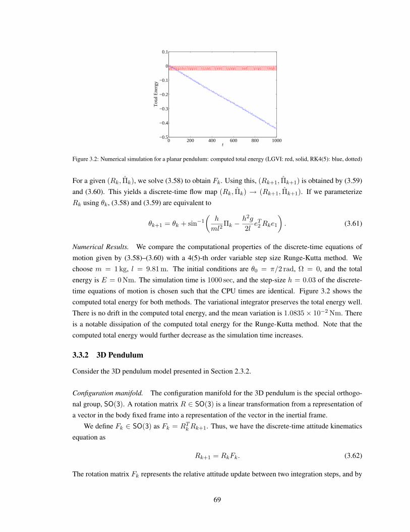
0 200 400 600 800 1000−0.5
−0.4
−0.3
−0.2
−0.1
0
0.1
t
Tot
al E
nerg
yFigure 3.2: Numerical simulation for a planar pendulum: computed total energy (LGVI: red, solid, RK4(5): blue, dotted)
For a given (Rk, Πk), we solve (3.58) to obtain Fk. Using this, (Rk+1, Πk+1) is obtained by (3.59)
and (3.60). This yields a discrete-time flow map (Rk, Πk) → (Rk+1, Πk+1). If we parameterize
Rk using θk, (3.58) and (3.59) are equivalent to
θk+1 = θk + sin−1
(h
ml2Πk −
h2g
2leT2 Rke1
). (3.61)
Numerical Results. We compare the computational properties of the discrete-time equations of
motion given by (3.58)–(3.60) with a 4(5)-th order variable step size Runge-Kutta method. We
choose m = 1 kg, l = 9.81 m. The initial conditions are θ0 = π/2 rad, Ω = 0, and the total
energy is E = 0 Nm. The simulation time is 1000 sec, and the step-size h = 0.03 of the discrete-
time equations of motion is chosen such that the CPU times are identical. Figure 3.2 shows the
computed total energy for both methods. The variational integrator preserves the total energy well.
There is no drift in the computed total energy, and the mean variation is 1.0835× 10⁻² Nm. There
is a notable dissipation of the computed total energy for the Runge-Kutta method. Note that the
computed total energy would further decrease as the simulation time increases.
3.3.2 3D Pendulum
Consider the 3D pendulum model presented in Section 2.3.2.
Configuration manifold. The configuration manifold for the 3D pendulum is the special orthogo-
nal group, SO(3). A rotation matrix R ∈ SO(3) is a linear transformation from a representation of
a vector in the body fixed frame into a representation of the vector in the inertial frame.
We define Fk ∈ SO(3) as Fk = RTkRk+1. Thus, we have the discrete-time attitude kinematics
equation as
Rk+1 = RkFk. (3.62)
The rotation matrix Fk represents the relative attitude update between two integration steps, and by
69

requiring that Fk lies on SO(3) we guarantee that the discrete flow Rk for k ∈ 0, . . . , N evolves
on SO(3) automatically.
The adjoint operator is as follows.
AdF η = F ηF T = F η, Ad∗F η = F T ηF = F T η (3.63)
for F ∈ SO(3), η ∈ so(3).
Discrete Lagrangian. Recall that the Lagrangian L : SO(3)×so(3)→ R of the attitude dynamics
of the 3D pendulum is given by
L(R, Ω) =12
tr[ΩJdΩT
]− U(R) (3.64)
for an attitude dependent gravitational potential U : SO(3)→ R.
Using the kinematics equations (2.48), (3.62), Ωk can be approximated as
Ωk = RTk Rk ≈1hRTk (Rk+1 −Rk) =
1h
(Fk − I). (3.65)
From the trapezoidal rule, we choose the following form of the discrete Lagrangian Ld : SO(3) ×SO(3)→ R.
Ld(Rk, Fk) =h
2L(Rk,
1h
(Fk − I)) +h
2L(Rk+1,
1h
(Fk − I))
=1
2htr[(Fk − I)Jd(Fk − I)T
]− h
2U(Rk)−
h
2U(Rk+1)
=1
2htr[FkJdF
Tk − FkJd − JdF Tk + Jd
]− h
2U(Rk)−
h
2U(Rk+1).
Since tr[FkJdF
Tk
]= tr
[JdF
Tk Fk
]= tr[Jd], and tr
[JdF
Tk
]= tr[FkJd], the discrete Lagrangian can
be written as
Ld(Rk, Fk) =1h
tr[(I − Fk)Jd]−h
2U(Rk)−
h
2U(RkFk). (3.66)
Discrete-time Euler-Lagrange Equations. We first find expressions for the derivatives of the dis-
crete Lagrangian. Let Td : SO(3)→ R be the first term of the discrete Lagrangian
Td(Fk) =1h
tr[(I − Fk)Jd] .
The derivative of Td(Fk) with respect to Fk is given by
DFkTd(Fk) · δFk = −1h
tr[δFkJd] · δFk = −1h
tr[FkF
Tk δFkJd
]= −1
htr[(F Tk δFk)(JdFk)
], (3.67)
70

where we use the property of the trace tr[AB] = tr[BA] for any A,B ∈ Rn×n. The following
identity is satisfied for any x ∈ R3, B ∈ R3×3, since tr[xB] = −tr[BT x
]= −tr
[xBT
]:
tr[xB] =12
tr[x(B −BT )
]= −
⟨B −BT , x
⟩. (3.68)
Since F Tk δFk is skew symmetric, (3.67) can be written as
DFkTd(Fk) · δFk = −1h
tr[δFkJd] =1h
⟨JdFk − F Tk Jd, F Tk δFk
⟩. (3.69)
As in (2.60), the derivative of the potential is given by
DRkU(Rk) · δRk = −⟨Mk, R
Tk δRk
⟩=
12
tr[MkR
Tk δRk
], (3.70)
where Mk is determined by Mk = ∂Uk∂Rk
RTk −Rk∂Uk∂Rk
T. Therefore, we have
DRkU(RkFk) · δRk =12
tr[Mk+1F
Tk R
Tk δRkFk
]=
12
tr[(RTk δRk)(FkMk+1F
Tk )]
= −⟨
FkMk+1, RTk δRk
⟩. (3.71)
Similarly, we also have
DFkU(RkFk) · δFk = −⟨Mk+1, F
Tk δFk
⟩. (3.72)
From (3.69), (3.70), (3.71), and (3.72), the derivatives of the discrete Lagrangian are given by
DFkLd(Rk, Fk) · δFk = DFkTd(Fk) · δFk −h
2DFkU(RkFk) · δFk
=⟨
1h
(JdFk − F Tk Jd) +h
2Mk+1, F
Tk δFk
⟩,
DRkLd(Rk, Fk) · δRK = −h2DRkU(Rk) · δRk −
h
2DRkU(RkFk) · δRk
=h
2
⟨Mk + FkMk+1, R
Tk δRk
⟩.
Therefore, we obtain
T∗eLFk ·DFkLd(Rk, Fk) =1h
(JdFk − F Tk Jd) +h
2Mk+1, (3.73)
Ad∗FTk+1
T∗eLFk+1·DFk+1
Ld(Rk+1, Fk+1) =1h
(Fk+1Jd − JdF Tk+1) +h
2Fk+1Mk+2, (3.74)
T∗eLRk+1·DRk+1
Ld(Rk+1, Fk+1) =h
2(Mk+1 + Fk+1Mk+2). (3.75)
Substituting these into (3.10) and (3.11), the discrete-time Euler-Lagrange equations for the 3D
71
pendulum are given by
1h
(Fk+1Jd − JdF Tk+1 − JdFk + F Tk Jd
)= hMk+1, (3.76)
Rk+1 = RkFk, (3.77)
where Mk = mgρc × RTk e3. For given (Rk, Rk+1) and Fk = RTkRk+1, we solve the implicit
equation (3.76) to find Fk+1. Then, Rk+2 is obtained from (3.77). This yields a discrete-time flow
map (Rk, Rk+1)→ (Rk+1, Rk+2), and this procedure is repeated.
Discrete Legendre Transformation. From (3.14), (3.15), the discrete Legendre transformation is
given by
Πk = −T∗eLRk ·DRkLd(Rk, Fk) + Ad∗FTk· T∗eLFk ·DFkLd(Rk, Fk)
=1h
(FkJd − JdF Tk )− h
2Mk, (3.78)
Πk+1 = T∗eLFk ·DFkLd(Rk, Fk)
=1h
(JdFk − F Tk Jd) +h
2Mk+1. (3.79)
Combining these, we have
Πk+1 =1hF Tk (FkJd − JdF Tk )Fk +
h
2Mk+1,
Πk+1 = F Tk ΠkFk +h
2Mk +
h
2Mk+1.
Using the fact that F T ΠF = F TΠ for any Π ∈ R3 and F ∈ SO(3), we obtain equivalent equations
in a vector form. In summary, the discrete-time Hamilton’s equations are given by
h(Πk +
h
2Mk
)∧ = FkJd − JdF Tk , (3.80)
Rk+1 = RkFk, (3.81)
Πk+1 = F Tk Πk +h
2F Tk Mk +
h
2Mk+1. (3.82)
For given (Rk,Πk), we solve the implicit equation (3.80) to find Fk. Then, Rk+1 is obtained from
(3.81), and Πk+1 is obtained from (3.82). This yields a discrete map (Rk,Πk) → (Rk+1,Πk+1),
and this procedure is repeated.
The discrete-time equations given by (3.76) and (3.80) are implicit equations: we need to solve
an implicit equation at each time step in order to find the relative update represented by the rota-
tion matrix Fk ∈ SO(3). A computational approach for these implicit equations is presented in
Section 3.3.8.
Remark 3.3 In this section, we have developed discrete-time Euler-Lagrange equations and discrete-
time Hamilton’s equations for the 3D pendulum by substituting the discrete Lagrangian given by
72

(3.66) into the discrete-time Euler-Lagrange equations on a general Lie group (3.10). Alternatively,
the discrete Euler-Lagrange equations for the 3D pendulum can be derived by following the pro-
cedure presented in Section 3.1.1. The corresponding discrete Hamilton’s principle on SO(3) has
been studied in Lee et al. (2005b).
Symmetry. Recall that the symmetry action of the 3D pendulum Φ : S1×SO(3)→ SO(3) is given
by
Φ(θ,R) = expSO(3)(θe3)R, (3.83)
which represents the rotation of the 3D pendulum about the gravity direction e3.
We first find expressions for the infinitesimal generators. We identify h = so(2) with R. From
(2.20), for ζ ∈ R, the infinitesimal generator ζSO(3) : SO(3)→ SO(3)× so(3) is given by
ζSO(3)(R) = φL d
dε
∣∣∣∣ε=0
ΦexpSO(2) εζ(R) = φL d
dε
∣∣∣∣ε=0
expSO(3)(εζe3)R
= φL (R, ζe3R) = (R, ζRT e3). (3.84)
From the definition (3.27), the infinitesimal generator ζSO(3)×SO(3) : SO(3)× SO(3)→ TSO(3)×TSO(3) is given by
ζSO(3)×SO(3)(Rk, Fk) =(TeLRk · ζSO(3)(Rk), TeLFk · (−AdFTk ζSO(3)(Rk) + ζSO(3)(RkFk))
)= ζ
(RkR
Tk e3, Fk(RTk+1e3 − F Tk RTk e3)∧
). (3.85)
Now we show that the discrete Lagrangian is infinitesimally invariant under the symmetry ac-
tion. From (3.22), (3.23), the discrete Lagrangian one-forms on SO(3)× SO(3) are given by
Θ+Ld
(Rk, Fk) · (δRk, δFk) =⟨T∗eLFk ·DFkLdk , F
Tk δFk + AdFTk ·R
Tk δRk
⟩=⟨
1h
(JdFk − F Tk Jd) +h
2Mk+1, F
Tk δFk + F Tk R
Tk δRkFk
⟩,
Θ−Ld(Rk, Fk) · (δRk, δFk) = −⟨T∗eLRk ·DRkLdk −Ad∗
FTk· (T∗eLFk ·DFkLdk), RTk δRk
⟩=⟨
1h
(FkJd − JdF Tk )− h
2Mk, R
Tk δRk
⟩.
Since Ldk = Θ+Ld−Θ−Ld , we obtain
Ld(Rk, Fk) · ζSO(3)×SO(3) = (Θ+Ld−Θ−Ld) · ζSO(3)×SO(3)
=⟨
1h
(JdFk − F Tk Jd) +h
2Mk+1, ζR
Tk+1e3
⟩−⟨
1h
(FkJd − JdF Tk )− h
2Mk, ζR
Tk e3
⟩.
73
Since Mk = mgρc ×RTk e3, we have⟨Mk, R
Tk e3
⟩= 0,
⟨Mk+1, R
Tk+1e3
⟩= 0. Thus, we obtain
Ld(Rk, Fk) · ζSO(3)×SO(3) =⟨
1h
(JdFk − F Tk Jd), ζRTk+1e3
⟩−⟨
1h
(FkJd − JdF Tk ), ζRTk e3
⟩=⟨
1h
(JdFk − F Tk Jd), ζRTk+1e3
⟩−⟨
1hF Tk (FkJd − JdF Tk )Fk, ζF Tk RTk e3Fk
⟩=⟨
1h
(JdFk − F Tk Jd), ζRTk+1e3
⟩−⟨
1h
(JdFk − F Tk Jd), ζ (FkRk)T e3
⟩= 0.
Therefore, the discrete Lagrangian is infinitesimally invariant under the symmetry action.
We now find an expression for the discrete momentum map. According to (3.28), the momentum
map J+Ld
: SO(3)× SO(3)→ R∗ is given by
J+Ld
(Rk, Fk) · ζ = Θ+Ld· ζG×G(Rk, Fk)
=⟨
1h
(JdFk − F Tk Jd) +h
2Mk+1, ζR
Tk+1e3
⟩=⟨
Πk+1, ζRTk+1e3
⟩= ζeT3 Rk+1Πk+1, (3.86)
where we use the discrete Legendre transformation (3.79). Thus, J+Ld
(Rk, Fk) = eT3 Rk+1Πk+1,
which represents the angular momentum of the 3D pendulum about the gravity direction. This is
preserved by the discrete-time flow according to the discrete Noether’s theorem.
Remark 3.4 The preservation of the angular momentum about the gravity direction can be directly
shown from (3.82). Multiplying the left and right sides of (3.82) by eT3 Rk+1, we obtain
eT3 Rk+1Πk+1 = eT3 Rk+1FTk Πk +
h
2eT3 Rk+1F
Tk Mk +
h
2eT3 Rk+1Mk+1
= eT3 RkFkΠk +h
2eT3 RkMk +
h
2eT3 Rk+1Mk+1.
Since eT3 RkMk = 0, eT3 Rk+1Mk+1 = 0, this reduces to
eT3 Rk+1Πk+1 = eT3 RkFkΠk,
which shows conservation of the momentum map by the discrete-time flow. This is a more concise
proof. The preceding development shows a formal application of the abstract discrete Noether’s
theorem to the 3D pendulum model.
Numerical Results. We compute the flow of discrete-time Hamilton’s equations. The physical
constants for the 3D pendulum are chosen as
m = 1 kg, ρc = [0, 0, 0.3] m, J = diag[0.13, 0.28, 0.17] kgm2.
74

0 20 40 60 80 100−10
0
10
0 20 40 60 80 100−10
0
10Ω
0 20 40 60 80 100−10
0
10
t
(a) Angular velocity Ω
0 20 40 60 80 1002.02
2.025
2.03
2.035
2.04
t
E
(b) Total energy E
0 20 40 60 80 1000
0.5
1
1.5
2
2.5
x 10−14
t
|I−R
T R
|
(c) Orthogonality error ‖I −RTR‖
0 20 40 60 80 100−6
−5
−4
−3
−2
−1
0
1x 10
−14
t
Δπ3
(d) Angular momentum error eT3 RkΠk − eT3 R0Π0
Figure 3.3: Numerical simulation for a 3D pendulum
Initial conditions are chosen as
R0 = I, Ω0 = [4.14, 4.14, 4.14] rad/s.
The simulation time and step size are tf = 100 seconds, h = 0.01 seconds.
Figure 3.3 shows responses of angular velocity of the pendulum, computed total energy, orthog-
onality error, and the deviation of the angular momentum along the gravity direction. As shown by
Figure 3.3(b), the computed total energy of the Lie group variational integrator oscillates near the
initial value, but there is no increasing or decreasing drift for long time periods. The orthogonality
error of rotation matrices and the error in conservation of the angular momentum about the gravity
direction remain at machine precision level.
75

3.3.3 3D Pendulum with an Internal Degree of Freedom
Consider the 3D pendulum with an internal degree of freedom presented in Section 2.3.3.
Configuration Manifold. The configuration manifold is SO(3) × R. The group action defines the
discrete-time update map as
(Rk+1, xk+1) = (Rk, xk)(Fk,∆xk)
= (RkFk, xk + ∆xk) (3.87)
for (Fk,∆xk) ∈ SO(3)× R. The Ad operator also has the product structure.
Ad(F,∆x)(η, x′) = (F ηF T , x′) = (F η, x′), Ad∗(F,∆x)(η, x
′) = (F T ηF, x′) = (F T η, x′).
Discrete Lagrangian. Recalling (2.75), the Lagrangian is given by
L(R, x,Ω, x) =12
ΩTJΩ +12mx(x2 − ρTx Ω2ρx + 2eT1 Q
T Ωρxx)
+mgeT3 Rρc +mxgeT3 Rρx −
12κx2.
The discrete Lagrangian is chosen as
Ld(Rk, xk, Fk,∆xk) =1h
tr[(I − Fk)Jd] +mx
2h∆x2
k −mx
2htr[ρxkρ
Txk
(Fk − I)2]
− mx
htr[Qe1∆xkρTxk(Fk − I)
]+h
2mgeT3 Rkρc +
h
2mxge
T3 Rkρxk
+h
2mgeT3 RkFkρc +
h
2mxge
T3 RkFkρxk+1
− h
4κx2
k −h
4κ(xk + ∆xk)2.
(3.88)
We find expressions for the derivatives of the discrete Lagrangian. The derivative of the discrete
Lagrangian with respect to Fk is given by
DFkLdk · δFk = −1h
tr[δFkJd]−mx
2htr[ρxkρ
Txk
(FkδFk + δFkFk − 2δFk)]
− mx
htr[Qe1∆xkρTxkδFk
]+h
2mgeT3 RkδFkρc +
h
2mxge
T3 RkδFkρxk+1
= −1h
tr[δFkAk] +h
2mgeT3 RkδFkρc +
h
2mxge
T3 RkδFkρxk+1
,
where Ak ∈ R3×3 is defined as
Ak = Jd +mx
2(ρxkρ
TxkFk + Fkρxkρ
Txk− 2ρxkρ
Txk
) +mxQe1∆xkρTxk .
76

This can be written as
DFkLdk · δFk = −1h
tr[(F Tk δFk)AkFk
]+h
2mgeT3 Rk+1(F Tk δFk)ρc
+h
2mxge
T3 Rk+1(F Tk δFk)ρxk+1
. (3.89)
Since F Tk δFk is skew symmetric, using (3.68), the first term of (3.89) can be written as
−1h
tr[(F Tk δFk)AkFk
]=
1h
⟨AkFk − F Tk ATk , F Tk δFk
⟩.
Since xy = −yx for any x, y ∈ R3, the last two terms of (3.89) can be written as
h
2mgeT3 Rk+1(F Tk δFk)ρc +
h
2mxge
T3 Rk+1(F Tk δFk)ρxk+1
= −h2mgeT3 Rk+1ρc(F Tk δFk)
∨ − h
2mxge
T3 Rk+1ρxk+1
(F Tk δFk)∨
=h
2⟨mgρcR
Tk+1e3 +mxgρxk+1
RTk+1e3, (F Tk δFk)∨⟩ . (3.90)
Therefore, we obtain
T∗eLFk ·DFkLdk =1h
(AkFk − F Tk ATk ) +(h
2mgρcR
Tk+1e3 +
h
2mxgρxk+1
RTk+1e3
)∧. (3.91)
The Ad∗ operation gives
Ad∗FTk· (T∗eLFk ·DFkLdk) =
1h
(FkAk −ATk F Tk )
+(h
2mgFkρcR
Tk+1e3 +
h
2mxgFkρxk+1
RTk+1e3
)∧. (3.92)
The derivative of the discrete Lagrangian with respect to Rk is given by
DRkLdk · δRk =h
2mgeT3 δRkρc +
h
2mxge
T3 δRkρxk +
h
2mgeT3 δRkFkρc +
h
2mxge
T3 δRkFkρxk+1
=h
2mgeT3 Rk(R
Tk δRk)ρc +
h
2mxge
T3 Rk(R
Tk δRk)ρxk
+h
2mgeT3 Rk(R
Tk δRk)Fkρc +
h
2mxge
T3 Rk(R
Tk δRk)Fkρxk+1
.
By following the same procedure used to derive (3.90), we obtain
T∗eLRk ·DRkLdk =h
2mgρcR
Tk e3 +
h
2mxgρxkR
Tk e3 +
h
2mgFkρcR
Tk+1e3 +
h
2mxgFkρxkR
Tk+1e3.
(3.93)
The derivative of the discrete Lagrangian with respect to ∆xk is given by
D∆xkLdk =mx
h∆xk −
mx
htr[Qe1ρ
Txk
(Fk − I)]
+h
2mxge
T3 Rk+1Qe1 −
h
2κxk+1. (3.94)
77
The Ad∗ operation is the identity on R. Since δρxk = Qe1δxk, the derivative of the discrete
Lagrangian with respect to xk is given by
DxkLdk = −mx
2htr[(Qe1ρ
Txk
+ ρxeT1 Q
T )(Fk − I)2 + 2∆xk(Fk − I)]
+h
2mxge
T3 RkQe1 +
h
2mxge
T3 Rk+1Qe1 −
h
2κxk −
h
2κxk+1. (3.95)
Discrete-time Euler-Lagrange Equations. We substitute (3.91)-(3.95) to (3.10) for gk = (Rk, xk)and fk = (Fk,∆xk) to obtain the discrete-time Euler-Lagrange equations
1h
(Ak−1Fk−1 − F Tk−1ATk−1 − FkAk +ATk F
Tk )∨
+ hmgρcRTk e3 + hmxgρxkR
Tk e3 = 0,
(3.96)
Ak = Jd +mx
2(ρxkρ
TxkFk + Fkρxkρ
Txk− 2ρxkρ
Txk
) +mxQe1∆xkρTxk , (3.97)
−mx
h(xk+1 − 2xk+xk−1)− mx
htr[Qe1ρ
Txk−1
(Fk−1 − I)]
+mx
htr[Qe1ρ
Txk
(Fk − I)]
− mx
2htr[(Qe1ρ
Txk
+ ρxeT1 Q
T )(Fk − I)2 + 2(xk+1 − xk)(Fk − I)]
+ hmxgeT3 RkQe1 − hκxk = 0.
(3.98)
Discrete-time Legendre Transformation. The discrete Legendre transformation yields the follow-
ing discrete-time Hamilton’s equations.
pΩk =1h
(FkAk −ATk F Tk )∨ − h
2mgρcR
Tk e3 −
h
2mxgρxkR
Tk e3, (3.99)
pxk =mx
h∆xk −
mx
htr[Qe1ρ
Txk
(Fk − I)]
+mx
2htr[(Qe1ρ
Txk
+ ρxeT1 Q
T )(Fk − I)2 + 2∆xk(Fk − I)]− h
2mxge
T3 RkQe1 +
h
2κxk,
(3.100)
Ak = Jd +mx
2(ρxkρ
TxkFk + Fkρxkρ
Txk− 2ρxkρ
Txk
) +mxQe1∆xkρTxk , (3.101)
pΩk+1=
1h
(AkFk − F Tk Ak)∨ +h
2mgρcR
Tk+1e3 +
h
2mxgρxk+1
RTk+1e3, (3.102)
pxk+1=mx
h∆xk −
mx
htr[Qe1ρ
Txk
(Fk − I)]
+h
2mxge
T3 Rk+1Qe1 −
h
2κxk+1. (3.103)
For given (Rk, xk,Ωk, xk), we find (pΩk , pxk) by (2.79). We use a fixed point iteration to deter-
mine Fk. For an initial guess of Fk, the corresponding ∆xk is determined from (3.100), and Akis determined from (3.101). Then, we can find Fk by solving (3.99). This is repeated until Fkconverges. (Rk+1, xk+1) are obtained from (3.87), and (pΩk+1
, pxk+1) are obtained from (3.102),
(3.103). The velocities (Ωk+1, xk+1) can be determined by (2.79). This yields a discrete-time flow
map (Rk, xk,Ωk, xk)→ (Rk+1, xk+1,Ωk+1, xk+1).
78

0 5 10 15 20 25 30−2
0
2
0 5 10 15 20 25 30−2
0
2Ω
0 5 10 15 20 25 30−2
0
2
t
(a) Angular velocity Ω
0 5 10 15 20 25 30−0.5
0
0.5
x
0 5 10 15 20 25 30−2
0
2
t
x
(b) Position and velocity of the par-ticle x, x
0 5 10 15 20 25 300
0.2
0.4
0.6
0.8
1
1.2
1.4x 10
−13
t
|I−R
T R
|
(c) Orthogonality error ‖I −RTR‖
Figure 3.4: Numerical simulation for a 3D pendulum with an internal degree of freedom
Numerical Results. We compute the flow of discrete-time Hamilton’s equations. The physical
constants for the 3D pendulum with an internal degree of freedom are chosen as
m = 1 kg, mx = 0.1 kg, ρc = [0, 0, 1] m, d = 0.15 m, κ = 1.1 N/m,
J = diag[1.03, 1.06, 0.05] kgm2, Q =
1.00 0.00 0.000.00 0.25 0.960.00 0.96 −0.25
.Initial conditions are chosen as
x0 = 0.10 m, x0 = 0.00 m/s,
R0 = exp(π
6e2), Ω0 = [0.1, 0.2, 1.0] rad/s.
Figure 3.4 shows responses of the angular velocity of the pendulum, the position of the particle
with respect to the 3D pendulum, and the velocity of the particle. The computed orthogonality error
of the rotation matrix is also shown.
3.3.4 3D Pendulum on a Cart
Consider the 3D pendulum whose pivot is attached to a cart moving on a horizontal plane, presented
in Section 2.3.4.
Configuration Manifold. The configuration manifold is SO(3)×R2. The group action defines the
discrete-time update map (3.11) as
(Rk+1, xk+1, yk+1) = (Rk, xk, yk)(Fk,∆xk,∆yk)
= (RkFk, xk + ∆xk, yk + ∆yk),
for (Fk,∆xk,∆yk) ∈ SO(3)× R2. The adjoint operator also has a product structure as follows
Ad(F,∆x,∆y)(η, x′, y′) = (F ηF T , x′, y′), Ad∗(F,∆x,∆y)(η, x
′, y′) = (F T ηF, x′, y′).
79

Discrete Lagrangian. Recalling (2.84), the Lagrangian is given by
L(R,Ω, x, y) =12
(M +m)(x2 + y2) +12
ΩTJΩ +mxeT1 Rρc +myeT2 Rρc +mgeT3 Rρc.
The discrete Lagrangian is chosen as
Ld(Rk, xk, yk, Fk,∆xk,∆yk) =1
2h(M +m)((∆xk)2 + (∆yk)2) +
1h
tr[(I − Fk)Jd]
+m
h∆xkeT1 Rk(Fk − I)ρc +
m
h∆ykeT2 Fk(Rk − I)ρc +
h
2mgeT3 Rkρc +
h
2mgeT3 RkFkρc.
(3.104)
We find the expressions for the derivatives of the discrete Lagrangian. We have
DFkLdk · δFk = −1h
tr[δFkJd] +m
h∆xkeT1 RkδFkρc +
m
h∆ykeT2 RkδFkρc +
h
2mgeT3 RkδFkρc
= −1h
tr[FkF
Tk δFkJd
]+m
h∆xkeT1 Rk+1F
Tk δFkρc +
m
h∆ykeT2 Rk+1F
Tk δFkρc
+h
2mgeT3 Rk+1F
Tk δFkρc. (3.105)
Since F Tk δFk is skew-symmetric, and using (3.68), the first term of (3.105) can be written as
−1h
tr[Fk(F Tk δFk)Jd
]= −1
htr[(F Tk δFk)JdFk
]=
1h
⟨JdFk − F Tk Jd, F Tk δFk
⟩.
We use the identity: for any x, y, z ∈ R3,
yT xz = −tr[yzT x
]=⟨yzT − zyT , x
⟩. (3.106)
Using (3.106), the second term of (3.105) can be written as
m
h∆xkeT1 Rk+1F
Tk δFkρc =
m
h∆xk
⟨RTk+1e1ρ
Tc − ρceT1 Rk+1, F
Tk δFk
⟩.
We apply the same identity to the remaining terms of (3.105) to obtain
T∗eLFk ·DFkLdk =1h
(JdFk − F Tk Jd) +m
h∆xk(RTk+1e1ρ
Tc − ρceT1 Rk+1)
+m
h∆yk(RTk+1e2ρ
Tc − ρceT2 Rk+1) +
h
2mg(RTk+1e3ρ
Tc − ρceT3 Rk+1).
(3.107)
Similarly, we obtain
T∗eLRk ·DRkLdk =m
h∆xk(RTk e1ρ
Tc (F Tk − I)− (Fk − I)ρce1Rk)
+m
h∆yk(RTk e2ρ
Tc (F Tk − I)− (Fk − I)ρce2Rk)
+h
2mg(RTk e3ρ
Tc − ρceT3 Rk) +
h
2mg(RTk e3ρ
Tc F
Tk − FkρceT3 Rk). (3.108)
80

We have Ad∗F−1k
(T∗eLFk · DFkLdk) = Fk(T∗eLFk · DFkLdk)F Tk . The derivatives of the discrete
Lagrangian with respect to ∆xk, ∆yk are given by
D∆xkLdk =1h
(M +m)∆xk +m
heT1 (Rk+1 −Rk)ρc, (3.109)
D∆ykLdk =1h
(M +m)∆yk +m
heT2 (Rk+1 −Rk)ρc. (3.110)
Discrete-time Euler-Lagrange Equations. Substituting (3.107)-(3.110) into (3.10), we obtain the
discrete Euler-Lagrange equations for the 3D pendulum on a cart.
1h
(M +m)(xk+1 − 2xk + xk−1) +m
heT1 (Rk+1 − 2Rk +Rk−1)ρc = 0, (3.111)
1h
(M +m)(yk+1 − 2yk + yk−1) +m
heT2 (Rk+1 − 2Rk +Rk−1)ρc = 0, (3.112)
1h
(FkJd − JdF Tk − JdFk−1 + F Tk−1Jd) = −mh
(xk+1 − 2xk + xk−1)(RTk e1ρTc − ρceT1 Rk)
− m
h(yk+1 − 2yk + yk−1)(RTk e2ρ
Tc − ρceT2 Rk) + hmg(RTk e3ρ
Tc − ρceT3 Rk).
(3.113)
Using the property x× y = yxT − xyT , the third equation can be written as
1h
(FkJd − JdF Tk − JdFk−1 + F Tk−1Jd)∨
= −mh
(xk+1 − 2xk + xk−1)ρcRTk e1 −m
h(yk+1 − 2yk + yk−1)ρcRTk e2 + hmgρcR
Tk e3.
(3.114)
Discrete-time Legendre Transformation. The discrete Legendre transformation yields the follow-
ing discrete-time Hamilton’s equations.
pxk =1h
(M +m)(xk+1 − xk) +m
he1(Rk+1 −Rk)ρc, (3.115)
pyk =1h
(M +m)(yk+1 − yk) +m
he2(Rk+1 −Rk)ρc, (3.116)
pΩk =1h
(FkJd − JdF Tk )
+m
h(xk+1 − xk)ρcRTk e1 +
m
h(yk+1 − yk)ρcRTk e2 −
h
2mgρcR
Tk e3
∧, (3.117)
Rk+1 = RkFk, (3.118)
pxk+1= pxk , (3.119)
pyk+1= pyk , (3.120)
pΩk+1=
1h
(JdFk − F Tk Jd)
+m
h(xk+1 − xk)ρcRTk+1e1 +
m
h(yk+1 − yk)ρcRTk+1e2 +
h
2mgρcR
Tk+1e3
∧.
(3.121)
81

For given (Rk, xk, yk,Ωk, xk, yk), we find (pΩk , pxk , pyk) by (2.90). We use a fixed point itera-
tion to determine Rk+1. For an initial guess of Rk+1, the corresponding xk+1, yk+1 are obtained
from (3.115), (3.116). Then, we can find Fk by solving (3.117). The new value for Rk+1 is
given by (3.118). This is repeated until Rk+1 converges. Then, xk+1, yk+1 are obtained from
(3.115), (3.116), and (pΩk+1, pxk+1
, pyk+1) are obtained by (3.119), (3.120), and (3.121). The
velocities (Ωk+1, xk+1, yk+1) can be obtained from (2.90). This yields a discrete-time flow map
(Rk, xk, yk,Ωk, xk, yk)→ (Rk+1, xk+1, yk+1,Ωk+1, xk+1, yk+1).
Numerical Results. We compare the computational properties of the discrete-time equations of
motion given by (3.115)-(3.121) with a 4(5)-th variables step size Runge-Kutta method. The physi-
cal constants for the 3D pendulum on a cart are chosen as
M = m = 1 kg, ρc = [0.25, 0.25, 1] m, J =
1.09 −0.06 −0.25−0.05 1.10 −0.25−0.25 −0.25 0.15
kgm2.
Initial conditions are chosen such that the mass center of the system is located at the origin, and the
total linear momentum is zero.
x0 = −0.125 m, x0 = 0.525 m/s, y0 = 0.5 m, y0 = −0.0125 m/s,
R0 =
1 0 00 0 −10 1 0
, Ω0 = [0.1, 0.2, 5.0] rad/s.
Figure 3.5(a) shows the computed total energy for 50 seconds. The Lie group variational inte-
grator preserves the total energy well. But there is a notable dissipation of the computed total energy
using the Runge-Kutta method. Similar characteristics are observed for the orthogonality error of
the rotation matrices in Figure 3.5(b).
It can be shown that the horizontal component of the total linear momentum is conserved. As
a result, the mass center moves along the vertical e3 axis, and the horizontal location of the mass
center of the system is fixed. Figure 3.5(c)-3.5(d) show the trajectory of the cart on the horizontal
plane, and Figure 3.5(e)-3.5(g) show the initial configuration and the configuration at t = 700 sec.
It is interesting to observe that the computed mass center of the Runge-Kutta method drifts in the
horizontal plane, as it does not preserve the total linear momentum properly.
82

0 10 20 30 40 50−1.12
−1.11
−1.1
−1.09
−1.08
−1.07
−1.06
t
E
(a) Computed total energy
0 10 20 30 40 5010
−20
10−15
10−10
10−5
100
t
|I−R
T R
|
(b) Orthogonality error ‖I −RTR‖
−0.6 −0.4 −0.2 0 0.2 0.4 0.6−0.5
0
0.5
x
y
(c) Trajectory of the cart (LGVI)
−2 −1.5 −1 −0.5 0 0.5 1
−2
−1.5
−1
−0.5
0
0.5
x
y
(d) Trajectory of the cart (RK4(5))
(e) Initial configuration (f) Configuration at t = 700s(LGVI)
(g) Configuration at t = 700s(RK4(5))
Figure 3.5: Numerical simulation for a 3D pendulum on a cart (LGVI: red, solid, RK4(5): blue, dotted)
83

3.3.5 Single Rigid Body
Consider a rigid body acting under a potential that is dependent of the attitude and the position of
the body, presented in Section 2.3.5.
Configuration Manifold. Let gk = (Rk, xk), fk = (Fk, Yk) ∈ SE(3) for Rk, Fk ∈ SO(3),
xk, Yk ∈ R3. The group action of SE(3) is matrix multiplication in homogeneous coordinates.
The discrete-time kinematics equation (3.11) can be written as[Rk+1 xk+1
0 1
]=
[Rk xk
0 1
][Fk Yk
0 1
]=
[RkFk xk +RkYk
0 1
]. (3.122)
The adjoint operator for SE(3) can be written in a matrix form as
Ad(R,x) =
[R 0xR R
], Ad∗(R,x) =
[RT −RT x0 RT
]. (3.123)
Discrete Lagrangian. The discrete Lagrangian is chosen as
Ld(gk, fk) = T (fk)−h
2U(gk)−
h
2U(gkfk), (3.124)
where the discrete kinetic energy term is defined as
T (fk) =1h〈〈fk − e, fk − e〉〉 =
m
2hYk · Yk +
1h
tr[(I3×3 − Fk)Jd] .
Thus, δT (fk) is given by
δT (fk) =m
hYk · δYk +
1h
tr[−δFkJd]
=m
hYk · δYk +
1h
tr[−F Tk δFJdFk
].
Since F Tk δFk is skew-symmetric, this can be rewritten as
δT (fk) =m
hF Tk Yk · F Tk δYk −
12h
tr[F Tk δF (JdFk − F Tk Jd)
]=
⟨[1h(JdFk − F Tk Jd)
mh F
Tk Yk
0 0
],
[F Tk δFk F Tk δYk
0 0
]⟩. (3.125)
Using (2.96) and (2.62), the derivatives of the potential term can be written as
−Dgk(U(gk) + U(gkfk)) · δgk −DfkU(gkfk) · δfk
=
[Mk −RTk
∂Uk∂xk
0 0
]· ηk +
[Mk+1 −RTk+1
∂Uk+1
∂xk+1
0 0
]· (Adf−1
kηk + f−1
k δfk). (3.126)
84

From (3.125) and (3.126), T∗eLfk ·DfkLd(gk, fk) is given by
T∗eLfk ·DfkLd(gk, fk) =
[1h(JdFk − F Tk Jd)
mh F
Tk Yk
0 0
]+
[h2Mk+1 −h
2RTk+1
∂Uk+1
∂xk+1
0 0
].
(3.127)
Using (3.123), Ad∗f−1k
(T∗eLfk ·DfkLd(gk, fk)) is computed in R6 as
Ad∗f−1k
(T∗eLfk ·DfkLd(gk, fk))
=
[Fk FkF
Tk Yk
0 Fk
][1h (JdFk − F Tk Jd)
mh F
Tk Yk
]+ Ad∗
f−1k
[h2Mk+1
h2 −R
Tk+1
∂Uk+1
∂xk+1
0 0
]
=
[1h (FkJd − JdF Tk )
mh Yk
]+ Ad∗
f−1k
[h2Mk+1 −h
2RTk+1
∂Uk+1
∂xk+1
0 0
]. (3.128)
An expression for T∗eLgk ·DgkLd(gk, fk) is obtained from (3.126).
T∗eLgk ·DgkLd(gk, fk) =
[h2Mk −h
2RTk∂Uk∂xk
0 0
]+ Ad∗
f−1k
[h2Mk+1 −h
2RTk+1
∂Uk+1
∂xk+1
0 0
]. (3.129)
Discrete-time Euler-Lagrange Equations. Substituting (3.127), (3.128), and (3.129) into (3.10),
JdFk−1 − F Tk−1Jd − (FkJd − JdF Tk ) + h2Mk = 0, (3.130)
m
h2F Tk−1Yk−1 −
m
h2Yk −RTk
∂Uk∂xk
= 0. (3.131)
Since the left-trivialization is used, these equations are expressed in the body fixed frame. From
(3.122), Yk = RTk (xk+1 − xk). Substituting this into the above equation, we obtain
m
h2F Tk−1R
Tk−1(xk − xk−1)− m
h2RTk (xk+1 − xk)−RTk
∂Uk∂xk
= 0.
Multiplying this by Rk, and rearranging, we obtain
m
h2(xk+1 − 2xk + xk−1) = −∂Uk
∂xk. (3.132)
Therefore, the discrete-time Euler-Lagrange equations are given by (3.130) and (3.132).
Discrete Legendre Transformation. Let (Πk,Γk) ∈ se(3)∗ be the angular momentum and the
linear momentum of the rigid body, represented with respect to the body fixed frame. From (3.14)
and (3.15), the discrete Legendre transformations are given by[Πk Γk0 0
]=
[1h(FkJd − JdF Tk )− h
2Mkmh Yk + h
2RTk∂Uk∂xk
0 0
],
85
[Πk+1 Γk+1
0 0
]=
[1h(JdFk − F Tk Jd)
mh F
Tk Yk
0 0
]+
[h2Mk+1 −h
2RTk+1
∂Uk+1
∂xk+1
0 0
].
It is desirable to express the discrete-time equations for the location and the linear momentum of
the rigid body with respect to the reference frame. Let γ ∈ R3∗ be the linear momentum represented
with respect to the reference frame, i.e. γ = RΓ. The discrete-time Hamilton’s equations can be
written as
hΠk +h2
2Mk = JdFk − F Tk Jd, (3.133)
Πk+1 = F Tk Πk +h
2F Tk Mk +
h
2Mk+1, (3.134)
xk+1 = xk +h
mγk −
h2
2m∂Uk∂xk
, (3.135)
γk+1 = γk −h
2∂Uk∂xk
− h
2∂Uk+1
∂xk+1. (3.136)
Numerical Results. We simulate the dynamics of a dumbbell body acting under a gravitational
potential from a fixed spherical body. We assume that the mass of the dumbbell is negligible com-
pared to the mass of the spherical body, and the origin of the reference frame is located at the mass
center of the spherical body. The gravitational potential results in a nontrivial coupling between the
attitude dynamics and the orbital dynamics. This model is referred to as a restricted full two body
problem.
The dumbbell model consists of two equal rigid spheres and a rigid massless connecting rod.
This dumbbell rigid body model results in a simple closed form for the mutual gravitational potential
given by
U(R, x) = −GMm
2
2∑q=1
‖x+Rρq‖,
where G is the universal gravitational constant, and M is the mass of the spherical body. The
constant m is the mass of the spherical body, and ρq ∈ R3 is a vector from the origin of the body-
fixed frame to the qth sphere of the dumbbell in the body-fixed frame.
We compare computational properties of the Lie group variational integrator with Runge-Kutta
methods applied to three types of attitude representations, namely, rotation matrices, quaternions,
and Euler-angles. The attitude kinematics equation is expressed in terms of quaternions and Euler-
angles, and the Runge-Kutta method is applied.
Figure 3.6 shows numerical simulation results for a near-circular orbit, where the trajectory of
the dumbbell, the angular velocity response, the computed total energy, and the orthogonality error
are presented. The Lie group variational integrator preserves the total energy and the Lie group
structure of SO(3). The mean total energy deviation is 2.5983× 10⁻⁴, and the mean orthogonality
error is 1.8553 × 10⁻¹³. But, there is a notable dissipation of the computed total energy and the
orthogonality error for the Runge-Kutta method.
86

(a) Trajectory of the dumbbell
0 20 40 60 80 1000.4917
0.4917
0.4917
0 20 40 60 80 100−5
0
5
Ω
0 20 40 60 80 100−5
0
5
t
(b) Angular velocity Ω
0 100 200 300 400 500−0.44
−0.435
−0.43
−0.425
−0.42
−0.415
−0.41
−0.405
t
Tot
al E
nerg
y
LGVI
RK.RotMat
RK.EulAng
RK.Quaternion
(c) Computed Total Energy
0 100 200 300 400 50010
−20
10−15
10−10
10−5
100
t
|I−R
T R
|
(d) Orthogonality Error ‖I −RTR‖
Figure 3.6: Numerical simulation for a single rigid body (Lie group variational integrator:LGVI, Runge-Kutta withrotation matrices:RK.RotMat, Runge-Kutta with Euler-angles:RK. EulAng, Runge-Kutta with quaternions:RK.qua
It is interesting to see that the Runge-Kutta method using quaternions, which is generally as-
sumed to have better computational properties than the kinematics equation with rotation matrices,
has a larger total energy error and a larger orthogonality error. Since the unit length of the quater-
nion vector is not preserved in the numerical computations, the orthogonality errors arise when
converted to a rotation matrix. This suggests that, even with conventional (non-geometric) inte-
grators, the rotation matrix has better computational properties than quaternions for the rigid body
dynamics.
87

3.3.6 Full Body Problem
Consider the full body problem presented in Section 2.3.6.
Discrete-time Euler-Lagrange Equations. The configuration manifold of the full n body problem
is (SE(3))n. Since the dynamics of the full body system are only coupled through the mutual
potential, the development for a single rigid body, presented in Section 3.3.5, is readily extended to
the full n body problem to obtain the discrete-time Euler-Lagrange equations.
JdiFik−1− F Tik−1
Jdi − (FkiJdi − JdiFTki
) + h2Mik = 0, (3.137)
mi
h2(xik+1
− 2xik + xik−1) = − ∂Uk
∂xik, (3.138)
where the subscript i refers to the i-th rigid body for i ∈ 1, . . . , n. Similarly, discrete-time
Hamilton’s equations given by (3.133)-(3.136) can be easily extended to the full n-body problem.
Discrete-time Reduced Euler-Lagrange Equations. When the mutual potential depends only on
the relative positions and the relative attitudes of rigid bodies, the Lagrangian is invariant under the
action of SE(3), and the configuration manifold can be reduced to a quotient space (SE(3))n−1.
Discrete-time reduced Euler-Lagrange equations for the full two body problem have been de-
veloped in Lee et al. (2007b,c). The procedure to derive discrete-time reduced Euler-Lagrange
equations is the same as the procedure presented in Section 3.1. The expressions for the variations
should be carefully developed for the reduced variables. Here, we present the resulting discrete-time
reduced Euler-Lagrange equations for the full two body problem. The detailed development can be
found in Lee et al. (2007c).
The discrete-time reduced Euler-Lagrange equations for the full two body problem are given by
F2kXk+1− 2X
k+ F T2k−1
Xk−1
= −h2
m
∂Uk
∂Xk
, (3.139)
Fk+1
JdRk+1− JdRk+1
F Tk+1
= F T2k(FkJdRk − JdRkF
Tk
)F2k − h
2Mk+1, (3.140)
F2k+1Jd2 − Jd2F T2k+1
= F T2k(F2kJd2 − Jd2F
T2k
)F2k + h2X
k+1× ∂U
∂Xk+1
+ h2Mk+1, (3.141)
Rk+1
= F T2kFkRk, (3.142)
R2k+1= R2kF2k . (3.143)
The discrete Legendre transformation yields the discrete-time Hamilton’s equations.
Xk+1
= F T2k
(Xk
+ hΓk
m− h2
2m∂U
k
∂Xk
), (3.144)
Γk+1
= F T2k
(Γk− h
2∂U
k
∂Xk
)− h
2∂U
k+1
∂Xk+1
, (3.145)
Πk+1
= F T2k
(Πk− h
2M
k
)− h
2M
k+1, (3.146)
88

Π2k+1= F T2k
(Π2k +
h
2Xk× ∂U
∂Xk
+h
2M
k
)+h
2Xk+1× ∂U
∂Xk+1
+h
2M
k+1, (3.147)
Rk+1
= F T2kFkRk, (3.148)
h
(Πk −
h
2M
k
)∧= F
kJdRk − JdRkF
Tk, (3.149)
h
(Π2k +
h
2Xk× ∂U
∂Xk
+h
2M
k
)∧= F2kJd2 − Jd2F
T2k, (3.150)
where the reduced variables for the linear momentum and the angular momentum are given by
Γ = mV , Π = JRΩ = RJ1Ω1, and Π2 = J2Ω2.
Numerical Results. We simulate the dynamics of two simple dumbbell bodies acting under their
mutual gravity. Each dumbbell model consists of two equal rigid spheres and a rigid massless
connecting rod. This dumbbell rigid body model results in a simple closed form for the mutual
gravitational potential given by
U(X,R) = −2∑
p,q=1
Gm1m2/4∥∥X + ρ2p +Rρ1q
∥∥ ,where G is the universal gravitational constant, mi ∈ R is the total mass of the ith dumbbell, and
ρip ∈ R3 is a vector from the origin of the body-fixed frame to the pth sphere of the ith dumbbell in
the ith body-fixed frame. The vectors ρi1 = [li/2, 0, 0]T , ρi2 = −ρi1 , where li is the length between
the two spheres.
The mass and length of the second dumbbell are twice that of the first dumbbell. The other
simulation parameters are chosen such that the total linear momentum in the inertial frame is zero
and the relative motion between the two bodies are near-elliptic orbits. The trajectories of the two
dumbbell bodies are shown in Figure 3.7(a).
We compare the computational properties of the Lie group variational integrator (LGVI) with
other second order numerical integration methods: an explicit Runge-Kutta method (RK), a sym-
plectic Runge-Kutta method (SRK), and a Lie group method (LGM). One of the distinct features of
the LGVI is that it preserves both the symplectic property and the Lie group structure for the full
rigid body dynamics. A comparison can be made between the LGVI and other integration methods
that preserve either none or one of these properties: an integrator that does not preserve any of these
properties (RK), a symplectic integrator that does not preserve the Lie group structure (SRK), and a
Lie group integrator that does not preserve symplecticity (LGM). These methods are implemented
by an explicit mid-point rule, an implicit mid-point rule, and the Crouch-Grossman method pre-
sented in Hairer et al. (2000) for the continuous equations of motion (2.108)–(2.113), respectively.
For the LGVI, the discrete-time equations of motion given by (3.144) through (3.150) are used. All
of these integrators are second order accurate. A comparison with a higher-order integrator can be
found in Fahnestock et al. (2006).
Figure 3.7(b) shows the computed total energy response over 30 seconds with an integration step
89

size h = 0.002 sec. For the LGVI, the total energy is nearly constant, and it has no tendency to drift;
while the other integrators fail to preserve the total energy. This can be observed in Figure 3.7(c),
where the mean total energy deviations are shown for varying integration step sizes. It is seen that
the total energy errors of the SRK method is close to the RK method, but the total energy error
of the LGVI is smaller by several orders. Figure 3.7(d) shows the mean orthogonality errors. The
LGVI and the LGM conserve the orthogonal structure at an error level of 10−10, while the RK and
the SRK are much less accurate.
These computational comparisons suggest that for numerical integration of Hamiltonian sys-
tems evolving on a Lie group, such as full body problems, it is critical to preserve both the symplec-
tic property and the Lie group structure. For the RK and the SRK, the orthogonality error in the ro-
tation matrix corrupts the attitude of the rigid bodies. The accumulation of this attitude degradation
results in significant errors in the computation of the gravitational forces and moments dependent
upon the position and the attitude, which affect the accuracy of the entire numerical simulation. The
LGM conserves the orthogonal structure of rotation matrices numerically, but it does not respect
the characteristics of the Hamiltonian dynamics properly as a non-symplectic integrator; this causes
a drift of the computed total energy. The LGVI is a geometrically exact integration method in the
sense that it preserves all of the geometric features of the full rigid body dynamics concurrently.
This verifies the superiority of the LGVI in terms of computational accuracy. The performance
advantages of the LGVI becomes even more dramatic as the simulation time is increased.
Computational efficiency is compared in Figure 3.7(e), where CPU times of all methods are
shown for varying step sizes. The SRK has the largest CPU time requiring solution of an implicit
equation in 36 variables at each integration step. The RK and the LGM require similar CPU times
since both are explicit. It is interesting to see that the implicit LGVI actually requires less CPU time
than the explicit methods RK and LGM. This follows from the fact that the second order explicit
methods RK and LGM require two evaluations of (2.108)–(2.113), including the expensive force
and moment computations at each step. The LGVI requires only one evaluation at each step in ad-
dition to the solution the implicit equation. The computational approach described in Section 3.3.8
is efficient for solving the implicit equation (3.149) and hence it takes less time than the evalua-
tion of (2.108)–(2.113). The difference is further increased as the rigid body model becomes more
complicated since it involves a larger computation burden in computing the gravitational forces and
moments. Based on these properties, we claim that the LGVI is almost explicit. This comparison
demonstrates the higher computational efficiency of the LGVI.
In summary, comparing both Figure 3.7(c) and 3.7(e), we see that the LGVI requires 16 times
less CPU time than the LGM, 35 times less CPU time than the RK, and 98 times less CPU time than
the SRK for similar total energy error in this computational example for the full body problem.
90

(a) Trajectories of two dumbbell bodies
0 20 40 60 80 100−0.1593
−0.1592
−0.1591
−0.159
−0.1589
−0.1588
−0.1587
t
E
RKSRKLGMLGVI
(b) Computed total energy for 30 seconds
10−4
10−3
10−2
10−8
10−6
10−4
10−2
Step size
mea
n |Δ
E|
(c) Mean total energy error |E − E0| vs. step size
10−4
10−3
10−2
10−15
10−10
10−5
100
Step size
mea
n |I−
RTR
|
(d) Mean orthogonality error ‖I −RTR‖ vs. step size
10−4
10−3
10−2
101
102
103
104
Step size
CPU
tim
e
(e) CPU time vs. step size
Figure 3.7: Numerical simulation for a full two body problem (Explicit Runge-Kutta:RK, symplectic Runge-Kutta:SRK,Lie group method:LGM, and Lie group variational integrator:LGVI )
91

3.3.7 Two Rigid Bodies Connected by a Ball Joint
Consider the two rigid bodies connected by a ball joint presented in Section 2.3.7.
Configuration Manifold. The configuration manifold is SO(3)×SO(3)×R3. The discrete update
map (3.11) can be written as
(R1k+1, R2k+1
, xk+1) = (R1k , R2k , xk)(F1k , F2k ,∆xk)
= (R1kF1k , R2kF2k , xk + ∆xk)
for (F1k , F2k ,∆xk) ∈ SO(3)× SO(3)× R3. The adjoint operator also has product structure.
Ad(F1,F2,x)(η1, η2, x′) = (F1η1F
T1 , F2η2F
T2 , x), Ad∗(F1,F2,x)(η1, η2, x
′) = (F T1 η1F1, FT2 η2F2, x).
Discrete Lagrangian. Recall that, from (2.114), the Lagrangian is given by
L(R1, R2, x,Ω1,Ω2, x) =12
(m1 +m2)x · x+12
Ω1 · J1Ω1 +12
Ω2 · J2Ω2
+ x · (m1R1Ω1d1 +m2R2Ω2d2)− U(R1, R2, x)
for a configuration dependent potential U : SO(3)× SO(3)× R3 → R.
For gk = (R1k , R2k , xk) and fk = (F1k , F2k ,∆xk), the discrete Lagrangian is chosen as
Ld(gk, fk) =m1 +m2
2h∆xk ·∆xk +
1h
tr[(I3×3 − F1k)Jd1 ] +1h
tr[(I3×3 − F2k)Jd2 ]
+1h
tr[m1R1k(F1k − I3×3)d1∆xTk
]+
1h
tr[m2R2k(F2k − I3×3)d2∆xTk
]− hU(gk).
We find the expressions for the derivatives of the discrete Lagrangian. Using the identity given in
(3.68), we obtain
δ(tr[(I3×3 − Fik)Jdi ]) = tr[−δFikJdi ] = tr[−F TikδFikJdiFik
]=⟨F TikδFik , JdiFik − F
TikJid⟩.
Similarly, we have
δ(tr[miRi(Fik − I3×3)di∆xTk
]) = −
⟨ηi,mi(Fik − I)di∆xTkRik −miR
Tik
∆xkdTi (F Tik − I)⟩
−⟨F TikδFik ,midi∆xTkRikFik −miF
TikRTik∆xkdTi
⟩+ ∆xTkmiRik(Fik − I)di.
From these, we have
T∗eLFik ·DFikLdk =
1h
(Jdi −midi∆xTkRik)Fik −1hF Tik (Jid −miR
Tik
∆xkdTi ),
Ad∗F−1ik
(T∗eLFik ·DFikLdk) = Fik(T∗eLFik ·DFik
Ldk)F Tik ,
92

T∗eLRik ·DRikLdk =
mi
hRTik∆xkdTi (F Tik − I)− mi
h(Fik − I)di∆xTkRik − hMik ,
Dxk+1Ldk =
1h
(m1 +m2)∆xk +m1
hR1k∆xkd1 +
m2
hR2k∆xkd2,
DxkLdk = −1h
(m1 +m2)∆xk −m1
hR1k(F1k − I)d1 −
m2
hR2k(F2k − I)d2 − h
∂Uk∂xk
.
Discrete Euler-Lagrange Equations. Substituting these into (3.10), we obtain the discrete Euler-
Lagrange equations for the two rigid bodies connected by a ball joint as
ATik+1Fik+1
− F Tik+1Aik+1
+AikFik − FTikATik = hBik + h2Mik , (3.151)
Aik = Jid −miRTik
(xk+1 − xk)dTi , (3.152)
Bik =mi
h(Fik − I)di(xk+1 − xk)TRik −
mi
hRTik(xk+1 − xk)dTi (F Tik − I), (3.153)
Rik+1= RikFik , (3.154)
1h
(m1 +m2)(xk+2 − 2xk+1 + xk) +m1
h(R1k+1
(F1k+1− 2I) +R1k)d1
+m2
h(R2k+1
(F2k+1− 2I) +R2k)d2 = −h∂Uk+1
∂xk+1
(3.155)
for i ∈ 1, 2. These equation can be solved by a fixed point iteration for xk+2. For given
(R1k , R2k , F1k , F2k , xk, xk+1), we guess xk+2. Then, Fik+1can be obtained by solving (3.151),
and Rik+1is obtained by (3.154). The new value of xk+2 is given by (3.155). This procedure is
repeated until xk+2 converges.
Discrete Legendre Transformation. Using the discrete Legendre transformation, the discrete equa-
tions of motion in Hamiltonian form are given by
pik =1h
(FikJdi − JdiFTik
) +mi
h(RTik(xk+1 − xk)dTi − di(xk+1 − xk)TRik) + hMk, (3.156)
pik+1= F Tik (pik −Bik − hMk), (3.157)
Bik =mi
h(Fik − I)di(xk+1 − xk)TRik −
mi
hRTik(xk+1 − xk)dTi (F Tik − I), (3.158)
p3k =1h
(m1 +m2)(xk+1 − xk) +m1
hR1k(F1k − I)d1 +
m2
hR2k(F2k − I)d2 − h
∂Uk∂xk
,
(3.159)
p3k+1= p3k − h
∂Uk∂xk
, (3.160)
Rik+1= RikFik (3.161)
for i ∈ 1, 2. For given (R1k , R2k , xk,Ω1k ,Ω2k , xk), we find (p1k , p2k , p3k) using (2.119). We
solve xk+1 iteratively: we guess xk+1, and solve (3.157) to obtain Fik+1. Then, the new value
of xk+1 is obtained by (3.159). This procedure is repeated until xk+1 converges. Then, pik+1
93

and p3k+1are obtained by (3.157) and (3.160), respectively, and R1k+1
, R2k+1are obtained by
(3.161). Using (2.119), we find (Ω1k+1,Ω2k+1
, xk+1). Thus, this yields a discrete-time flow map
(R1k , R2k , xk,Ω1k ,Ω2k , xk) → (R1k+1, R2k+1
, xk+1,Ω1k+1,Ω2k+1
, xk+1), and this process is re-
peated.
Numerical Results. We assume there is no potential field, U ≡ 0. We choose two elliptic cylinder
rigid bodies with different shapes. The properties of the rigid bodies are given by
m1 = 2km, J1 = diag[0.1000, 1.1558, 1.2358]kgm2, d1 = [−0.75, 0, 0]m, (3.162)
m1 = 1km, J2 = diag[0.0325, 0.2200, 0.2325]kgm2, d2 = [0.45, 0, 0]m. (3.163)
The initial conditions are chosen such that the total linear momentum is zero.
R10 = I, Ω10 = [0, 0.5, 0]rad/s, R20 = I, Ω20 = [1, 0, 0]rad/s,
x0 = [0.35, 0, 0]m, x0 = [0, 0,−0.25]m/s.
Figure 3.8 shows the computed total energy, total linear momentum, and total angular mo-
mentum for the Lie group variational integrator and a 4(5)-th order variable step size Runge-Kutta
method. Since there is no potential, the total linear/anguar momentum should be preserved. The
Lie group variational integrators preserve the conserved quantities numerically, but there is notable
dissipation for the Runge-Kutta method.
94

(a) Two rigid bodies connected by a ball joint
0 10 20 30 40 500.0669
0.067
0.0671
0.0672
t
E
(b) Computed total energy
0 10 20 30 40 50−5
0
5x 10
−4
0 10 20 30 40 50−2
0
2x 10
−3
γT
0 10 20 30 40 50−5
0
5x 10
−4
t
(c) Computed total linear momentum
0 10 20 30 40 500.0324
0.0325
0.0326
0 10 20 30 40 500.315
0.3155
0.316
πT
0 10 20 30 40 50−2
0
2x 10
−4
t
(d) Computed total angular momentum
Figure 3.8: Numerical simulation for two rigid bodies connect by a ball joint (LGVI: red, solid, RK4(5): blue, dotted)
95

3.3.8 Computational Approach
Most of the discrete-time Euler-Lagrange equations presented in this section include implicit equa-
tions. In particular, we need to find the relative update of the group elements represented by the
group action of fk ∈ G at each discrete time step. Since the implicit equations are solved repeatedly
at each time step, it is important to develop a fast computational algorithm for overall computational
efficiency of the presented discrete Euler-Lagrange equations.
The essential idea is expressing the group element fk ∈ G in terms of a Lie algebra element
using the exponential map. The exponential map is a local diffeomorphism from the Lie algebra
g near zero to the Lie group G near the identity element. Since fk represents the relative update
between two adjacent integration steps, it is close to the identity. Therefore, the implicit equations
can be expressed at the Lie algebra level.
This is desirable since the Lie algebra is a linear vector space. The implicit equation is solved
numerically in the linear space, and the corresponding group element is obtained by the exponential
map. Since the solution of the implicit equation is close to zero in the Lie algebra, the implicit
equation is easily solved as the step size is decreased.
In this section, we present a computational approach to solve the implicit equation on SO(3)appearing in the discrete-time Euler-Lagrange equations for the 3D pendulum. This is the simplest,
but nontrivial, form of the implicit equation. The computational approach for other mechanical
systems can be obtained by extending the approach.
The discrete-time Euler-Lagrange equations (3.76) and the discrete-time Hamilton equations
(3.80) have the following form of the implicit equation; for given a ∈ R3 and Jd ∈ R3×3, we need
to find F ∈ SO(3) satisfying
a = FJd − JdF T . (3.164)
We rewrite this equation on R3 ' so(3) using the exponential map and the Cayley transformation,
to which a Newton iteration method is applied.
Exponential map
The exponential map on SO(3) has a closed form expression, referred to as Rodrigues’ formula (see
Marsden and Ratiu 1999):
F = exp f = I3×3 +sin ‖f‖‖f‖
f +1− cos ‖f‖‖f‖2
f2 (3.165)
for f ∈ R3. This physically represents the rotation about the axis f with the rotation angle ‖f‖.Substituting (3.165) into (3.164) and using the properties fJd + Jdf = Jf , f Jf − Jf f =
f × Jf , we obtain
a =sin ‖f‖‖f‖
Jf +1− cos ‖f‖‖f‖2
f × Jf.
96

Thus, (3.80) is converted into an equivalent vector equation in R3 as
0 = −a+sin ‖f‖‖f‖
Jf +1− cos ‖f‖‖f‖2
f × Jf ≡ A(f), (3.166)
where A : R3 → R3. We use the Newton method to solve this nonlinear vector equation 0 = A(f).
We use the following iteration formula iteration
f (i+1) = f (i) −∇A(f (i))−1A(f (i)), (3.167)
where the Jacobian∇A(f) in (3.167) can be expressed as
∇A(f) =cos ‖f‖ ‖f‖ − sin ‖f‖
‖f‖3JffT +
sin ‖f‖‖f‖
J
+sin ‖f‖ ‖f‖ − 2(1− cos ‖f‖)
‖f‖4(f × Jf) fT +
1− cos ‖f‖‖f‖2
−Jf + fJ
.
We iterate until∥∥f (i+1) − f (i)
∥∥ < ε for a given tolerance ε, and we find the rotation matrix F using
Rodrigues’ formula (3.165). The initial guess can be selected as the solution of the linearized vector
equation (3.166), which gives f (0) = J−1a, or the solution at the previous time step can be used as
the initial guess for the current step.
The implicit equation (3.166) expressed in R3 using the exponential map is well defined, since
the rotation matrix F represents the relative attitude update near the identity matrix. This computa-
tional approach technically avoids the nonlinear constraints associated with the rotation matrix F ;
the equivalent vector equation is iterated in R3.
However, the complicated expression for the Jacobian written in terms of trigonometric func-
tions may not be desirable for overall computational efficiency. Thus, we present another compu-
tational approach using the Cayley transformation. This approach reduces the computational load
using a numerically-efficient local diffeomorphism; the essential idea of solving an equivalent vec-
tor equation in R3 is the same as before.
Cayley transformation
The Cayley transformation is a local diffeomorphism between SO(3) and R3 given by
F = Cay(fc) = (I + fc)(I − fc)−1 = (I − fc)−1(I + fc)
=1
1 + fTc fc((1− fTc fc)I + 2fc + 2fcfTc ) (3.168)
for fc ∈ R3. This represents a rotation of a rigid body along the direction fc/ ‖fc‖ with rotation
angle θ determined by ‖fc‖ = tan θ2 . It can be shown that exp f = Cay(tan ‖f‖2
f‖f‖). Thus,
the Cayley transformation can be considered to be a modification of the exponential map, where
the rotation angle is encoded in a different way. But, the Cayley transformation has the numerical
advantage that it does not require evaluation of computationally-expensive sin and cos terms.
97

Using the Cayley transformation, we transform the implicit equation (3.164) into an equivalent
vector equation. Since the two matrices (I + fc) and (I − fc)−1 commute, we can write the Cayley
transformation in the following form for convenience.
F = Cay(fc) =I + fc
I − fc.
Substituting this into (3.164), we obtain
a =I + fc
I − fcJd − Jd
I − fcI + fc
.
Multiplying this by I − fc on the left side, by I + fc on the right side, we have
(I − fc)a(I + fc) = (I + fc)Jd(I + fc)− (I − fc)Jd(I − fc),
a+ a× fc − fcafc = fcJd + Jdfc + fcJd + Jdfc.
Using the following identities
fc × a = fca− afc, Jfc = Jdfc + fcJd, fcafc = −(aT fc)fc,
we obtain
(a+ a× fc + fc(aT fc))∧ = 2Jfc.
Therefore, (3.164) is converted into an equivalent vector equation in R3 as
0 = a+ a× fc + fc(aT fc)− 2Jfc ≡ Ac(fc). (3.169)
whereAc : R3 → R3. We use a Newton iteration to solve this nonlinear vector equation 0 = Ac(f).
We use the following iteration
f (i+1)c = f (i)
c −∇Ac(f (i)c )−1Ac(f (i)
c ), (3.170)
where the Jacobian∇Ac(fc) is given by
∇Ac(fc) = a+ (aT fc)I + fcaT − 2J. (3.171)
We iterate until∥∥f (i+1) − f (i)
∥∥ < ε for a given tolerance ε, and we find the rotation matrix using
the Cayley transformation (3.168). The initial guess can be selected as the solution of the linearized
vector equation of (3.169), which gives f (0)c = (2J − a)−1a, or the solution from the previous time
step can be used as the initial guess for the current step.
98

3.3.9 Summary of Computational Properties
We have derived discrete-time Euler-Lagrange equations for several rigid body systems evolving on
a Lie group, and computational results are presented. Here, we summarize the computational prop-
erties of the Lie group variational integrator compared to other numerical integrators for dynamics
of rigid bodies.
Computational Accuracy. The Lie group variational integrators preserve the geometric properties
of mechanical systems on a Lie group. In particular, the computed total energy, momentum map,
and deviation from the Lie group configuration manifold are presented. As shown at Figure 3.2,
3.3(b), 3.5(a), 3.6(c), 3.7(b), and 3.8(b), the computed total energy of the Lie group variational
integrator oscillates near the initial value, but there is no increasing or decreasing drift for long time
periods. This is due to the fact that the numerical solutions of symplectic numerical integrators
are the exact solution of a perturbed Hamiltonian (see Hairer 1994). The perturbed value of the
Hamiltonian is preserved in the discrete-time flow. This is in contrast to other numerical integrators
evaluated in this dissertation, such as the explicit Runge-Kutta method, the symplectic Runge-Kutta
method, and (non-symplectic) Lie group methods, where the computed total energy increases (or
decreases) linearly with the simulation time.
The Lie group variational integrators preserves the momentum map exactly as discussed in
Section 3.1.3. This can be observed in Figure 3.3(d), 3.8(c) and 3.8(d), where the value of the
momentum map is preserved up to machine precision. From the numerical simulation of the 3D
pendulum on a cart in Figure 3.5(c), the mass center of the system is fixed in space, since the Lie
group variational integrator conserves the zero value of the total linear momentum. But the location
of the mass center for the explicit Runge-Kutta method drifts, as shown at Figure 3.5(d), since it
does not accurately preserve the total linear momentum. Comparing the terminal configurations of
both methods in Figure 3.5(f) and Figure 3.5(g), we see that the computational results obtained by
the explicit Runge-Kutta method are not reliable.
The structure of the Lie group configuration manifold is well preserved in the Lie group varia-
tional integrator. As shown in Figure 3.4(c), 3.5(b), 3.6(d) and 3.7(d), the deviation of the discrete-
time flow from the Lie group, measured by the orthogonality error∥∥I −RTR∥∥, remains at machine
precision. But interestingly, the orthogonality error increases linearly with respect to the simulation
time, and accordingly, the mean orthogonality error increases as the time step decreases for a fixed
simulation time. This is due to the accumulation of roundoff errors. For example, since the rota-
tion matrix in SO(3) is updated by the group action of SO(3), which is matrix multiplication, the
k-th rotation matrix is obtained by k matrix multiplications, i.e. Rk = R0F0 · · ·Fk−1. The round-
off error at each matrix multiplication accumulates, and therefore the orthogonality error increases
linearly. The roundoff errors are unavoidable in any numerical computation with a finite digit rep-
resentation, and they are usually indiscernible. Here we can actually observe the accumulation of
roundoff errors, since there is no source for the orthogonality error except the roundoff errors in the
numerical computations. The magnitude of the orthogonality error is acceptable for any practical
99

purpose. In summary, the Lie group variational integrators preserve the Lie group structure up to
roundoff errors. The explicit Runge-Kutta method and the symplectic Runge-Kutta method do not
preserve the structure of the Lie group. As shown at Figure 3.5(b) and 3.7(d), the orthogonality
error for these methods are about 1010 times larger than the Lie group variational integrators, and
consequently, the attitude of the rigid body is not computed accurately.
In summary, the Lie group variational integrators are geometrically accurate numerical integra-
tors in the sense that they preserve all of the geometric properties of the dynamics of rigid bodies,
such as symplecticity, momentum map, total energy, and Lie group structure.
Computational Efficiency. In Section 3.3.8, computational approaches to solve the implicit equa-
tions in the Lie group variational integrator are developed. The essential idea is to write the implicit
equations in terms of a Lie algebra element using the exponential map, and numerically solve the
transformed implicit equation in a vector space. The corresponding computational requirements
are much smaller than for the fully-implicit symplectic Runge-Kutta method. In Section 3.3.6, we
have shown that if the discrete Lagrangian is carefully chosen to minimize the number of function
evaluations at each step, then the computational requirements of the Lie group variational integrator
are comparable to the explicit integrators for the same step size. Therefore, we claim the Lie group
variational integrator is almost explicit.
For the same level of total energy error, the Lie group variational integrators are faster than the
explicit Runge-Kutta method, the symplectic Runge-Kutta method, and the Lie group method by
several times. This computational advantage is due to the fact that latter integrators do not preserve
all, or one, of the symplecticity and the Lie group structure of the rigid body dynamics.
The RATTLE algorithm is a symplectic numerical integrator for a constrained Hamiltonian
system (see Leimkuhler and Reich 2004). By considering the orthogonal structure of the rotation
matrix as a nonlinear constraint, one can construct a symplectic numerical integrator that preserves
orthogonality using the RATTLE algorithm. A numerical comparison for the 3D pendulum model
shows that the Lie group variational integrator is faster than the RATTLE algorithm by 17-60%.
This illustrates that it is more efficient to expressing the relative update of group elements in terms
of the Lie algebra elements as proposed in this dissertation, than considering the group structure as
a nonlinear constraint that should be satisfied at each integration step.
In summary, the Lie group variational integrators have similar computational requirements com-
pared to other explicit numerical integrators for the same step size, and they are substantially more
efficient than other numerical integrator for the same level of numerical accuracy.
100

3.4 Examples of Mechanical Systems on Two-Spheres
Several mechanical systems evolving on a product of two-spheres have been introduced in Sec-
tion 2.4, and the corresponding expressions for inertia matrix, potential, and equations of motion
were presented. For the mechanical systems whose Lagrangian is expressed as (2.26), the expres-
sions for the inertia and the potential determine the corresponding discrete-time Euler-Lagrange
equations according (3.40), (3.52), (3.53), and (3.54). Therefore, the discrete-time Euler-Lagrange
equations for the mechanical systems presented in Section 2.4 have already been obtained. In this
section, computational results for the discrete-time Euler-Lagrange equations on two-spheres are
presented.
Section Mechanical System
3.4.1 Double Spherical Pendulum
3.4.2 n-body Problem on a Sphere
3.4.3 Interconnection of Spherical Pendula
3.4.4 Pure Bending of Elastic Rod
3.4.5 Spatial Array of Magnetic Dipoles
3.4.6 Molecular Dynamics on a Sphere
3.4.1 Double Spherical Pendulum
Consider the double spherical pendulum presented in Section 2.4.1. Recall that the inertia matrix is
given by M11 = (m1 +m2)l21, M12 = m2l1l2, and M22 = m2l22, and the gravitational potential is
written as U(q1, q2) = −(m1 +m2)gl1e3 · q1−m2gl2e3 · q2. Substituting these into (3.49)–(3.52),
the discrete-time equations of motion for the double spherical pendulum are given by
(m1 +m2)l21q1k × F1kq1k + q1k ×m2l1l2(F2k − I)q2k
= (m1 +m2)l21hω1k − q1k ×m2l1l2(q2k × hω2k) +h2
2q1k × (m1 +m2)gl1e3,
(3.172)
m2l22q2k × F2kq1k + q2k ×m2l1l2(F1k − I)q1k
= m2l22hω2k − q2k ×m2l1l2(q1k × hω1k) +
h2
2q1k ×m2gl2e3,
(3.173)
q1k+1= F1kq1k , q2k+1
= F2kq2k , (3.174)[(m1 +m2)l21I3×3 −m2l1l2q1k+1
q2k+1
−m2l1l2q2k+1q1k+1
m2l22I3×3
][ω1k+1
ω2k+1
]
=
[1hq1k+1
×m2l1l2(q2k+1− q2k) + h
2 q1k+1× (m1 +m2)gl1e3
1hq2k+1
×m2l1l2(q1k+1− q1k) + h
2 q2k+1×m2gl2e3
].
(3.175)
We compare the computational properties of the discrete-time equations of motion with a 4(5)-
th order variable step size Runge-Kutta method for (2.124)–(2.123). We choose m1 = m2 = 1 kg,
l1 = l2 = 9.81 m. The initial conditions are q10 = [0.8660, 0, 0.5], q20 = [0, 0, 1], ω10 =
101

(a) Trajectory of pendulum
0 20 40 60 80 100−0.7505
−0.75
−0.7495
−0.749
−0.7485
−0.748
t
E
(b) Computed total energy
0 20 40 60 80 10014.7145
14.715
14.7155
14.716
14.7165
14.717
14.7175
14.718
14.7185
t
π3
(c) Total angular momentum about the gravity direc-tion
0 20 40 60 80 10010
−20
10−15
10−10
10−5
100
t
|qT q
−1|
(d) Unit length error
Figure 3.9: Numerical simulation for a double spherical pendulum (RK45: blue, dotted, VI: red, solid)
[−0.4330, 0, 0.75], ω20 = [0, 1, 0] rad/sec. The simulation time is 100 sec, and the step size of the
discrete-time equations of motion is h = 0.01. Figure 3.9 shows the computed total energy and the
configuration manifold errors. The variational integrator preserves the total energy and the structure
of (S2)n well for this chaotic motion of the double spherical pendulum. The mean total energy
variation is 2.1641×10⁻⁵ Nm, and the mean unit length error is 8.8893×10⁻¹⁵. There is a notable
increase of the computed total energy for the Runge-Kutta method, where the mean variation of
the total energy is 7.8586 × 10⁻⁴ Nm. The mean deviations of the angular momentum about the
gravity direction are 1.0217 × 10⁻¹⁰ kgm2/s for the variational integrator, and 8.0497 × 10⁻⁴ for
the Runge-Kutta method, respectively. The Runge-Kutta method also fails to preserve the structure
of (S2)n. The mean unit length error is 6.2742× 10⁻⁵.
3.4.2 n-body Problem on a Sphere
Consider the n-body problem on a sphere presented in Section 2.4.2. It deals with the motion of n
mass particles constrained to lie on a two-sphere, acting under a mutual potential. Recall that the
102

(a) Trajectory of particles
10−4
10−3
10−2
10−1
10−6
10−5
10−4
10−3
10−2
10−1
Step size
Tot
al E
nerg
y E
rror
(b) Total energy error v.s. step size
10−4
10−3
10−2
10−1
10−15
10−10
10−5
Step size
Uni
t len
gth
Err
or
(c) Unit length error v.s. step size
Figure 3.10: Numerical simulation for a 3-body problem on sphere (RK2: blue, square, VI: red, circle)
inertia matrix is given byMij = mi when i = j, and Mij = 0 otherwise, and the gravitational
potential is given by U(q1, . . . , qn) = −γ2
∑j 6=i
qi·qj√1−(qi·qj)2
. Substituting these into (3.53)–(3.54),
the discrete-time equations of motion are given by
qik+1=(hωik −
h2
2miqik ×
∂Uk∂qik
)× qik +
(1−
∥∥∥∥hωik − h2
2miqik ×
∂Uk∂qik
∥∥∥∥2)1/2
qik , (3.176)
ωik+1= ωik −
h
2miqik ×
∂Uk∂qik
− h
2miqik+1
× ∂Uk+1
∂qik+1
, (3.177)
where
∂Uk∂qik
= −γn∑j=1j 6=i
qjk(1− (qik · qjk)2)3/2
.
A two-body problem on the two-sphere under this gravitational potential is studied in Hairer
et al. (2003) by explicitly using unit length constraints. Here we study a three-body problem, n = 3.
Since there are no coupling terms in the kinetic energy, we use the explicit form of the variational
integrator. We compare the computational properties of the discrete-time equations of motion with
a 2-nd order fixed step size Runge-Kutta method for (2.125). We choose m1 = m2 = m3 = 1,
and γ = 1. The initial conditions are q10 = [0, −1, 0], q20 = [0, 0, 1], q30 = [−1, 0, 0], ω10 =[0, 0, −1.1], ω20 = [1, 0, 0], and ω30 = [0, 1, 0]. The simulation time is 10 sec. Figure 3.10
shows the computed total energy and the unit length errors for various step sizes. The total energy
variations and the unit length errors for the variational integrator are smaller than those of the Runge-
Kutta method for the same step size by several orders of magnitude. For the variational integrator,
the total energy error is reduced by almost 100 times from 1.1717 × 10⁻⁴ to 1.1986 × 10⁻⁶ when
the step size is reduced by 10 times from 10−3 to 10−4, which verifies the second order accuracy
numerically.
103

(a) Motion of pendula
0 5 10 15 20 25 30−0.313
−0.3128
−0.3126
−0.3124
−0.3122
−0.312
t
E
(b) Computed total energy
0 5 10 15 20 25 3010
−20
10−15
10−10
10−5
100
t
|qT q
−1|
(c) Unit length error
Figure 3.11: Numerical simulation for an interconnection of 4 spherical pendula (RK2: blue, dotted, RK2 withprojection: black, dashed, VI: red, solid)
3.4.3 Interconnection of Spherical Pendula
Consider the interconnection of spherical pendula presented in Section 2.4.3. Recall that the inertia
matrix is given by Mij = mil2i when i = j, and Mij = 0 otherwise, and the potential is given by
U(q1, . . . qn) = −n∑i=1
migliqi · e3 +∑
(i,j)∈Ξ
12κij
(∥∥∥∥rij +12ljqj −
12liqi
∥∥∥∥− ‖rij‖)2
.
Substituting these into (3.53)–(3.54), the discrete-time equations of motion are given by
qik+1=(hωik −
h2
2mil2iqik ×
∂Uk∂qik
)× qik +
(1−
∥∥∥∥hωik − h2
2mil2iqik ×
∂Uk∂qik
∥∥∥∥2)1/2
qik ,
(3.178)
ωik+1= ωik −
h
2mil2iqik ×
∂Uk∂qik
− h
2mil2iqik+1
× ∂Uk+1
∂qik+1
. (3.179)
We compare the computational properties of the discrete-time equations of motion with a 2-
nd order fixed step size explicit Runge-Kutta method for (2.126)–(2.127), and the same Runge-
Kutta method with reprojection; at each time step, the vectors qik are projected onto S2 by using
normalization.
We choose four interconnected pendula, n = 4, and we assume each pendulum has the same
mass and length; mi = 0.1 kg, li = 0.1 m. A set Ξ is defined such that (i, j) ∈ Ξ if the i-th
pendulum and the j-th pendulum are connected. We choose Ξ = (1, 2), (2, 3), (3, 4), (4, 1), and
the corresponding spring constants and the relative vector between pivots are given by κ12 = 10,
κ12 = 20, κ12 = 30, κ12 = 40 N/m, r12 = −r34 = lie1, and r23 = −r41 = −lie2. The initial
conditions are chosen as q10 = q20 = q40 = e3, q30 = [0.4698, 0.1710, 0.8660], ω10 = [−10, 4, 0],and ω20 = ω30 = ω40 = 0 rad/sec
Figure 3.11 shows the computed total energy and the unit length errors. The variational inte-
grator preserves the total energy and the structure of (S2)n well. The mean total energy variation
is 3.6171 × 10⁻⁵ Nm, and the mean unit length error is 4.2712 × 10⁻¹⁵. For both Runge-Kutta
104

(a) Deformation of rod
0 0.5 1 1.5 2 2.5 30.0132
0.0134
0.0136
0.0138
0.014
0.0142
0.0144
t
E
(b) Computed total energy
0 0.5 1 1.5 2 2.5 310
−20
10−15
10−10
10−5
100
t
|qT q
−1|
(c) Unit length error
Figure 3.12: Numerical simulation for an elastic rod (RK45: blue, dotted, VI: red, solid)
methods, there is a notable increase of the computed total energy. It is interesting to see that the re-
projection approach increases the total energy error, even though it preserves the structure of (S2)n
accurately. This shows that a standard reprojection method can significantly corrupt numerical tra-
jectories (see Hairer et al. 2000; Lewis and Nigam 2003).
3.4.4 Pure Bending of Elastic Rod
Consider the pure bending motion of a slender elastic rod presented in Section 2.4.4. Recall that the
moment of inertia matrix is given by
Mii =13mil
2i +
n∑p=i+1
mpl2i ,
Mij =12
n∑p=i+1
2mpljli
+miljli
for 1 ≤ i < j ≤ n, and the potential is given by
U(q1, . . . , qn) =n∑i=1
−mig
i−1∑j=1
qjlj +12liqi
· e3 +EI
4l2i(1− qi−1 · qi)
.Substituting these into (3.49)–(3.52), we obtain the discrete-time equations of motion.
We compare the computational properties of the discrete-time equations of motion with a 4(5)-
th order variable step size Runge-Kutta method. We choose 10 rod elements, n = 10, and the
total mass and the total length are m = 55 g, l = 1.1,m. The spring constants are chosen as
κi = 1000 Nm. Initially, the rod is aligned horizontally; qi0 = e1 for all i ∈ 1, . . . n. The initial
angular velocity for each rod element is zero except ω50 = [0, 0, 10] rad/sec. This represents
the dynamics of the rod after an initial impact. The simulation time is 3 sec, and the step size is
h = 0.0001.
Figure 3.12 shows the computed total energy and the unit length errors. The variational in-
tegrator preserves the total energy and the structure of (S2)n. The mean total energy variation is
105
1.4310×10⁻⁶ Nm, and the mean unit length error is 2.9747×10⁻¹⁴. There is a notable dissipation
of the computed total energy for the Runge-Kutta method, where the mean variation of the total
energy is 3.5244× 10⁻⁴ Nm. The Runge-Kutta method also fail to preserve the structure of (S2)n.
The mean unit length error is 1.8725× 10⁻⁵.
3.4.5 Spatial Array of Magnetic Dipoles
Consider the spatial array of magnetic dipoles presented in Section 2.4.5. Recall that the inertia
matrix is given by Mij = 112mil
2i when i = j, and Mij = 0 otherwise. The magnetic potential is
given by
U(q1, . . . , qn) =12
n∑i,j=1j 6=i
µ νiνj4π‖rij‖3
[(qi · qj)−
3‖rij‖2
(qi · rij)(qj · rij)],
Substituting these into (3.53)–(3.54), we obtain the discrete-time Euler-Lagrange equations as
qik+1=(hωik −
6h2
mil2iqik ×
∂Uk∂qik
)× qik +
(1−
∥∥∥∥hωik − 6h2
mil2iqik ×
∂Uk∂qik
∥∥∥∥2)1/2
qik , (3.180)
ωik+1= ωik −
6hmil2i
qik ×∂Uk∂qik
− 6hmil2i
qik+1× ∂Uk+1
∂qik+1
, (3.181)
where
∂Uk∂qik
=n∑j=1j 6=i
µ νiνj4π‖rij‖3
[qj −
3‖rij‖2
rij(qj · rij)].
We compare the computational properties of the discrete-time equations of motion with a 4(5)-th
order variable step size Runge-Kutta method for (2.136)–(2.137). We choose 16 magnetic dipoles,
n = 16, and we assume each magnetic dipole has the same mass, length, and magnitude of magnetic
moment; mi = 0.05 kg, li = 0.02 m, νi = 0.1 A ·m2. The magnetic dipoles are located at vertices
of a 4 × 4 square grid in which the edge of a unit square has the length of 1.2li. The initial
conditions are chosen as qi0 = [1, 0, 0], ωi0 = [0, 0, 0] for all i ∈ 1, . . . , 16 except q160 =[0.3536, 0.3536,−0.8660] and ω10 = [0, 0.5, 0] rad/sec.
Figure 3.13 shows the computed total energy and the unit length errors. The variational inte-
grator preserves the total energy and the structure of (S2)n well. The mean total energy variation
is 8.5403× 10⁻¹⁰ Nm, and the mean unit length error is 1.6140× 10⁻¹⁴. There is a notable dissi-
pation of the computed total energy for the Runge-Kutta method, where the mean variation of the
total energy is 2.9989 × 10⁻⁷ Nm. The Runge-Kutta method also fail to preserve the structure of
(S2)n. The mean unit length error is 1.7594× 10⁻⁴.
106

(a) Motion of magnetic dipoles
0 5 10 15 20 25 30−1.2446
−1.2444
−1.2442
−1.244
−1.2438
−1.2436x 10
−3
t
E
(b) Computed total energy
0 5 10 15 20 25 3010
−20
10−15
10−10
10−5
100
t
|qT q
−1|
(c) Unit length error
Figure 3.13: Numerical simulation for an array of magnetic dipoles (RK45: blue, dotted, VI: red, solid)
3.4.6 Molecular Dynamics on a Sphere
Consider the molecular dynamics model on S2 presented in Section 2.4.6. Recall that the inertia
matrix is Mij = mi when i = j, and Mij = 0 otherwise. The Lennard-Jones potential is given by
U(q1, . . . , qn) =12
n∑i,j=1j 6=i
4ε
[(σ
‖qi − qj‖
)12
−(
σ
‖qi − qj‖
)6],
Substituting these into (3.53)–(3.54), we obtain the discrete-time Euler-Lagrange equations as
qik+1=(hωik −
h2
2mil2iqik ×
∂Uk∂qik
)× qik +
(1−
∥∥∥∥hωik − h2
2mil2iqik ×
∂Uk∂qik
∥∥∥∥2)1/2
qik ,
(3.182)
ωik+1= ωik −
h
2mil2iqik ×
∂Uk∂qik
− h
2mil2iqik+1
× ∂Uk+1
∂qik+1
, (3.183)
where
∂Uk∂qik
= −n∑j=1j 6=i
4εqi − qj‖qi − qj‖
[12σ12
‖qi − qj‖13 −6σ6
‖qi − qj‖7
].
We choose 642 molecules, n = 642, and we assume each molecule has the same mass, mi = 1.
Initially, molecules are uniformly distributed on a sphere. The strength of the potential is chosen
as ε = 0.01, and the constant σ is chosen such that the inter-molecular force between neighbor-
ing molecules is close to zero. The initial velocities are modeled as two vortices separated by
30 degrees. The simulation time is 5 s, and the step size is h = 0.005.
Trajectories of molecules and the computed total energy are shown in Figure 3.14. The mean
deviation of the total energy is 1.8893× 10⁻³, and the mean unit length error is 5.2623× 10⁻¹⁵. In
molecular dynamics simulations, macroscopic quantities such as temperature and pressure are more
useful than trajectories of individual molecules. Figure 3.15 shows the change of kinetic energy
distributions over time, which measures the temperature (see Allen and Tildesley 1987); the sphere
107

(a) Initial trajectories
0 1 2 3 4 5−6.6
−6.5875
−6.575
t
E
(b) Computed total energy
Figure 3.14: Numerical simulation for molecular dynamics on a sphere
(a) t = 0 (b) t = 0.25 (c) t = 0.5 (d) t = 0.75 (e) t = 5
Figure 3.15: Numerical simulation for molecular dynamics on a sphere: kinetic energy distributions over time
is discretized by an icosahedron with 5120 triangular faces, and the color of a face is determined by
the average kinetic energy for molecules that lie within the face and within its neighboring faces.
The local kinetic energy is represented by color shading of blue, green, yellow, and red colors in
ascending order.
3.4.7 Computational Approach
For the discrete equations of motion, we need to solve (3.40) and (3.49) to obtain Fik ∈ SO(3).
Here we present a computational approach. The implicit equations given by (3.40) and (3.49) have
the following structure.
Miiqi × Fiqi + qi ×n∑j=1j 6=i
Mij(Fj − I3×3)qj = di (3.184)
for i ∈ 1, . . . , n, where Mij ∈ R, qi ∈ S2, di ∈ R3 are known, and we need to find Fi ∈ SO(3).
We derive an equivalent equation in terms of local coordinates for Fi. This is reasonable since Firepresents the relative update between two integration steps. But, the solution is not unique since if
Fi ∈ SO(3) satisfies (3.184), then Fi exp(θqi) ∈ SO(3) also satisfies (3.184) for any θ ∈ S1. To
avoid this ambiguity, we search a 2-dimensional subgroup of SO(3) in which the solution of (3.184)
is unique.
Similar to the computational approach to solve the implicit equation of the Lie group variational
integrator on SO(3) presented in Section 3.3.8, the essential idea is to express the rotation matrix
108

Fi in terms of fi ∈ R3 using the the Cayley transformation. Using the Cayley transformation,
Fi ∈ SO(3) can be expressed in terms of fi ∈ R3 as
Fi = (I3×3 + fi)(I3×3 − fi)−1
=1
1 + fi · fi((1− fi · fi)I3×3 + 2fifTi + 2fi).
The operation Fiqi can be considered as a rotation of the vector qi about the direction fi with rotation
angle 2 tan−1 ‖fi‖. Since the rotation of the vector qi about the direction qi has no effect, we can
assume that fi is orthogonal to qi, i.e. fi · qi = 0. Under this assumption, Fiqi is given by
Fiqi =1
1 + fi · fi((1− fi · fi)qi + 2fiqi). (3.185)
Thus, we obtain
qi × Fiqi =2
1 + fi · fiqi × (fi × qi) =
21 + fi · fi
fi,
(Fj − I3×3)qj = − 21 + fj · fj
(qjfTj + qj)fj ,
where we use the property, qifi = qi × fi = −fiqi. Substituting these into (3.184), we obtain2M11I3×3
1+f1·f1 −2M12q1(q2+q2fT2 )1+f2·f2 · · · −2M1nq1(qn+qnfTn )
1+fn·fn−2M21q2(q1+q1fT1 )
1+f1·f12M22I3×3
1+f2·f2 · · · −2M2nq2(qn+qnfTn )1+fn·fn
......
...
−2Mn1qn(q1+q1fT1 )1+f1·f1 −2Mn2qn(q2+q2fT2 )
1+f2·f2 · · · 2MnnI3×3
1+fn·fn
f1
f2
...
fn
=
d1
d2
...
dn
, (3.186)
which is an equation equivalent to (3.184), written in terms of local coordinates for Fi using the
Cayley transformation. Any standard numerical method to solve nonlinear equations can be applied
to find fi. Then, Fiqi is computed by using (3.185). In particular, (3.186) is written in a form for
which a fixed point iteration method can be readily applied (see Kelley 1995).
If there are no coupling terms in the kinetic energy, we can obtain an explicit solution of (3.184).
When Mij = 0 for i 6= j, (3.186) reduces to
2Mii
1 + fi · fifi = di.
Using the identity, 2 tan θ1+tan2 θ
= sin 2θ for any θ ∈ R, it can be shown that the solution of this equation
is given by fi = tan(
12 sin−1(‖di‖ /Mii)
)di‖di‖ . Substituting this into (3.185) and rearranging, we
obtain
Fiqi =diMii× qi +
(1−
∥∥∥∥ diMii
∥∥∥∥2)1/2
qi.
Using this expression, we can rewrite the discrete-time equations of motion given by (3.49)–(3.52)
109

in an explicit form as in Corollary 3.5.
3.4.8 Summary of Computational Properties
We have derived discrete-time Euler-Lagrange equations for several dynamic systems evolving on
a product of two-spheres, and some computational results are presented. Here, we summarize the
computational properties of the Lie homogeneous variational integrator compared to other numeri-
cal integrators.
Computational Accuracy. Similar to the Lie group variational integrator, the distinct feature of
the Lie homogeneous variational integrators is that they preserve the symplecticity as well as the
structure of the two-spheres. As shown at Figure 3.9(b), 3.11(b), 3.12(b), 3.13(b), and 3.14(b), the
computed total energy of the Lie homogeneous variational integrator oscillates around the initial
value, but there is no drift on long time scales. The computed total energy of the explicit Runge-
Kutta methods increases (or decreases) linearly with respect to the simulation time. As a result, the
total energy deviation for the Runge-Kutta method is larger than the Lie homogeneous variational
integrator by several times as seen in Figure 3.10(b). We find a similar property for the momentum
map at Figure 3.9(c). Figure 3.9(d), 3.11(c), 3.12(c), and 3.13(c) show that the unit length error of
the Lie homogeneous variational integrator is at the level of 10−14–10−15, but the unit length error
of the explicit Runge-Kutta method is almost 1010 times larger.
In summary, the Lie homogeneous variational integrators are geometrically accurate in the sense
that they preserve all of the geometric properties of the dynamics, such as symplecticity, momentum
map, total energy, and the structure of the two-spheres.
Computational Efficiency. We have shown that if the inertia matrix for the kinetic energy is di-
agonal, the Lie homogeneous variational integrator becomes explicit. In this case, the variational
integrator given in Corollary 3.5 is faster than the explicit Runge-Kutta method with the same sec-
ond order accuracy, as it requires one-time evaluation of the potential derivatives per time step.
The RATTLE algorithm is a symplectic numerical integrator for a constrained Hamiltonian sys-
tem (see Leimkuhler and Reich 2004). By considering the unit norm structure of the two-sphere as a
nonlinear constraint, one can construct a symplectic numerical integrator evolving on two-spheres.
It turns out that the variational integrator given at Corollary 3.4 is equivalent to the RATTLE al-
gorithm if the computational implementational details are ignored. But, rather than imposing the
constraint on the unit length at each time step, we present a computational algorithm to update the
element of the two-sphere using the group action of SO(3).
The purpose of this section is to provide a systematic method to derive a geometric numerical
integrator evolving on a homogeneous space. The specific form of the discrete Lagrangian given
in (3.33) yields an equivalent expression to the RATTLE algorithm. But, it can be extended in
various ways, such as a configuration dependent inertia or an abstract homogeneous manifold, by
following the approach presented in this section. The presented computational approach is generally
110
slower than the RATTLE algorithm, but it represents a specific numerical method that updates an
element of a homogeneous space using the corresponding Lie group action explicitly. In particular,
a subgroup that guarantees the transitivity property is found for overall efficiency.
In summary, the presented form of the Lie homogeneous variational integrator is more numeri-
cally efficient if the inertia matrix is diagonal. It may be slightly slower than the RATTLE algorithm
using the presented computational algorithm. But, the computational approach provides an explicit
method to generalize the current results to mechanical systems evolving on an abstract homoge-
neous manifold.
3.5 Conclusions
In this chapter, geometric numerical integrators, referred to as Lie group variational integrators,
are developed for dynamic systems with a Lie group configuration manifold. The presented method
represents the first time that the Lie group approach is explicitly adopted in the context of variational
integrators for an arbitrary Lie group. They provide a systematic way to develop a class of geometric
numerical integrators that preserve the geometric properties of the dynamics as well as the Lie group
structure.
Numerical simulations in Section 3.3 show that it is critical to preserve both the symplectic
property of dynamics and the structure of the Lie group. The Lie group variational integrators have
substantial computational advantages compared to other geometric integrators that preserve either
none or one of these properties. They are more efficient than considering the Lie group structure as
a nonlinear algebraic constraint to be satisfied at each time step.
Compared with other geometric integrators for a rigid body, as in the work of Hulbert (1992);
Krysl (2005); Lewis and Simo (1994); Simo and Wong (1991), the Lie group variational integra-
tor provides a systematic method to obtain a class of numerical integrators that preserve all of the
geometric features, rather than developing a specific numerical integrator that preserves only a few
geometric characteristics. Compared with discrete-time mechanics on a Lie group developed by
Bobenko and Suris (1999); Marsden et al. (1999); Moser and Veselov (1991), the Lie group varia-
tional integrator can be applied to a wide class of rigid body dynamics acting under a potential field
as shown in Section 3.3.
These results are extended to mechanical systems on a product of two-spheres, to obtain Lie
homogeneous variational integrators in Section 3.2. They preserve the geometric feature of dynam-
ics as well as the structure of the two-spheres. Other geometric numerical integrators on S2 are
developed for a kinematics equations, and they do not necessarily preserve the symplectic property
or momentum map (see Lewis and Nigam 2003; Lewis and Olver 2001; Munthe-Kaas and Zanna
1997). The development in Section 3.2 also provides an overall framework to construct variational
integrators for dynamic systems on an abstract homogeneous manifold.
111

CHAPTER 4
GEOMETRIC OPTIMAL CONTROL OF RIGID BODIES ON ALIE GROUP
In this chapter, we formulate optimal control problems for mechanical systems that evolve on a
Lie group, and we derive necessary conditions for optimality. These results are illustrated by several
rigid body systems introduced in the previous chapters. This chapter is focused on developing
an intrinsic form of optimality conditions in continuous-time. Computational approaches to find
optimal control inputs are discussed in the next chapter.
4.1 Geometric optimal control on a Lie group
4.1.1 Forced Euler-Lagrange equations
4.1.2 Optimal control problem formulation
4.1.3 Necessary conditions for optimality
4.2 Examples of optimal control of rigid bodies
4.2.1 Spacecraft on a circular orbit
4.2.2 Free rigid body
4.2.3 3D Pendulum with symmetry
4.2.4 Rigid body under potential field
This chapter is organized as follows. In Section 4.1, we develop geometric optimal control
theory for dynamics on an arbitrary Lie group; the Euler-Lagrange equations derived in Chapter 2
are extended to include the effect of external control inputs, a general form of an optimal control
problem is formulated, and necessary conditions for optimality are developed. In Section 4.2, these
results are applied to several optimal control problems for rigid body dynamics.
4.1 Geometric Optimal Control on a Lie Group
Optimal control problems deal with finding trajectories, such that a certain optimality condition is
satisfied under prescribed constraints (see, for example, Bryson and Ho 1975; Kirk 1970; Sussmann
and Willems 1997). For example, a minimum time optimal control problem is studied for a space-
craft to change its attitude in a desired way while minimizing the maneuver time, and subject to
bounded control moments.
Geometric optimal control on a Lie group has been studied by Baillieul (1978); Bloch and
112

Crouch (1996); Brockett (1972); Jurdjevic (1998a,b, 1997) (see also references therein). But, these
approaches are based on kinematics equations on a Lie group, and assume that group elements are
directly controlled by control input elements in the Lie algebra. For example, an optimal attitude
control problem of a rigid body is considered in Jurdjevic (1997) by viewing the angular velocity to
be a control input.
This chapter deals with optimal control problems of dynamic systems with a Lie group config-
uration manifold. More precisely, it may be considered as an optimal control problem on a tangent
bundle of a Lie group G, identified with G × g by left trivialization. For example, in Section 4.2.2,
we consider an optimal attitude control problem of a rigid body controlled by an external moment.
Another distinct feature of the presented geometric optimal control theory is that it is a coordinate-
free approach. Most of the prior work related to optimal control problems of a rigid body is based
on local coordinates of SO(3), such as Euler angles, or on quaternions (see, for example, Bilimoria
and Wie 1993; Byers and Vadali 1993; Scrivener and Thompson 1994; Seywald and Kumar 1993).
Here, we develop an intrinsic form of optimal control problems and necessary conditions. Optimal-
ity conditions and the resulting optimal control input are independent of the choice of representation
for the rigid body configuration. They are globally represented by group elements without any sin-
gularity and ambiguity, and the optimality conditions are more compact than expressions written in
terms of local parameterizations.
In summary, we develop a geometric optimal control theory to treat optimal control problems
for dynamic systems on a Lie group, expressed in a coordinate-free form. The geometric optimal
control approach is based on the Lagrangian mechanics on a Lie group presented in Chapter 2;
necessary conditions for optimality are derived using variational arguments. Here, we first extend
the Euler-Lagrange equations to include the effect of control inputs, and we formulate optimal
control problems for controlled Euler-Lagrange systems on a Lie group.
4.1.1 Forced Euler-Lagrange Equations on a Lie Group
Consider a mechanical system evolving on a Lie group G. As discussed in Chapter 2, we assume
that a Lagrangian of the system is expressed as L(g, ξ) : G×g→ R by left-trivialization, ξ = g−1g.
Suppose that there exists a generalized force u(t) : [t0, tf ] → g∗ acting on the system. Forced
Euler-Lagrange equations are obtained according to the Lagrange-d’Alembert principle:
δ
∫ tf
t0
L(g, ξ) dt+∫ tf
t0
u(t) · η dt = 0 (4.1)
for any η = g−1δg ∈ g vanishing at the endpoints. This is equivalent to Hamilton’s principle with
the additional forcing term. From (2.8), this can be written as∫ tf
t0
⟨T∗eLg ·DgL(g, ξ) + ad∗ξ ·DξL(g, ξ), η
⟩−⟨d
dtDξL(g, ξ), η
⟩+ 〈u, η〉 dt = 0,
which yields the forced Euler-Lagrange equations on G.
113

Proposition 4.1 Consider a mechanical system evolving on a Lie group G. We identify the tangent
bundle TG with G × g by left-trivialization. Suppose that the Lagrangian is defined as L(g, ξ) :G × g → R, and there exists a generalized force u : [t0, tf ] → g∗ acting on the system. The
corresponding forced Euler-Lagrange equations are given by
d
dtDξL(g, ξ)− ad∗ξ ·DξL(g, ξ)− T∗eLg ·DgL(g, ξ) = u, (4.2)
g = gξ. (4.3)
Special Form of Forced Euler-Lagrange Equations. Proposition 4.1 gives the forced Euler-Lagrange
equations for mechanical systems evolving on a Lie group G for a general form of the Lagrangian.
While it is possible to formulate an optimal control problem and derive necessary optimality condi-
tions for these systems, we consider mechanical systems with a structured form of the Lagrangian.
This allows us to obtain a more compact form of necessary conditions in Section 4.1.3.
Let J : g → g∗ be the inertia operator, which is linear, positive definite, and symmetric. More
explicitly, it satisfies
〈J(ξ), ξ〉 > 0, (4.4)
J(c1ξ1 + c2ξ2) = c1J(ξ1) + c2J(ξ2), (4.5)
〈J(ξ1), ξ2〉 = 〈J(ξ2), ξ1〉 , (4.6)
for any c1, c2 ∈ R, ξ 6= 0, ξ1, ξ2 ∈ g.
We assume that the Lagrangian is the difference between a kinetic energy, expressed in term of
the inertia operator, and a configuration dependent potential U : G→ R, given by
L(g, ξ) =12〈J(ξ), ξ〉 − U(g). (4.7)
We apply Proposition 4.1 to this Lagrangian. The derivatives of the Lagrangian are given by
DξL(g, ξ) · δξ =12〈J(δξ), ξ〉+
12〈J(ξ), δξ〉 = 〈J(ξ), δξ〉 ,
T∗eLg ·DgL(g, ξ) = −T∗eLg ·DgU(g) ≡M(g),
where the force due to the potential is denoted by M : G → g∗. Then, the forced Euler-Lagrange
equations reduce to the following.
Corollary 4.1 Consider a mechanical system evolving on a Lie group G. We identify the tangent
bundle TG with G × g by left-trivialization. Suppose that the Lagrangian is given by (4.7) for a
positive definite, symmetric, and linear inertia operator J : g→ g∗ and the configuration dependent
potential U : G → R. There exists a force u : [t0, tf ] → g∗ acting on the system. Then, the
114

corresponding forced Euler-Lagrange equations are given by
d
dtJ(ξ)− ad∗ξ · J(ξ)−M(g) = u, (4.8)
g = gξ, (4.9)
where the force due to the potential M : G→ g∗ is given by M(g) = −T∗eLg ·DgU(g).
4.1.2 Optimal Control Problem Formulation
We consider an optimal control problem for forced Euler-Lagrange systems described by Corollary
4.1. The optimal control problem is to find the control input that minimizes the following cost
functional:
J =∫ tf
t0
φ(g(t), ξ(t), u(t)) dt,
where φ : G × g × g∗ → R is given. Several types of boundary conditions can be considered:
free terminal time, fixed terminal time, free terminal conditions, fixed terminal conditions, and
terminal states lying on a given surface. Additionally, equality constraints or inequality constraints
may be imposed on the trajectory of the mechanical system and the control input. For simplicity,
here we consider optimal control problems with a free terminal time and fixed terminal conditions.
The optimal control problem with a fixed final time and fixed terminal conditions is considered as a
special case. The subsequent development can be easily extended to other optimal control problems.
The optimal control problem is summarized as follows.
For given t0, g(t0), ξ(t0), gf , ξf
minu(t),tf
J =
∫ tf
t0
φ(g(t), ξ(t), u(t)) dt,
such that g(tf ) = gf , ξ(tf ) = ξf ,
subject to the Euler-Lagrange equations (4.8), (4.9).
4.1.3 Necessary Conditions for Optimality
We derive necessary conditions for optimality using the calculus of variations: the Euler-Lagrange
equations are constrained by using Lagrange multipliers, and the variation of the corresponding
augmented cost functional is set to zero. The resulting necessary conditions are expressed as a two
point boundary value problem.
More explicitly, define the augmented cost functional:
Ja =∫ tf
t0
φ(g, ξ, u) +⟨d
dtJ(ξ)− ad∗ξJ(ξ)−M(g)− u, λ1
⟩+⟨λ2, g−1g − ξ
⟩dt, (4.10)
where λ1 ∈ g, λ2 ∈ g∗ are Lagrange multipliers. The variation of the augmented cost functional
115

is composed of two terms: the term due to the the terminal time variation and the term due to the
variation of trajectories for a fixed terminal time:
δJa = δJ 1a + δJ 2
a .
The variation of the augmented cost functional due to the terminal time change is given by
δJ 1a =
[φ(g, ξ, u) +
⟨d
dtJ(ξ)− ad∗ξJ(ξ)−M(g)− u, λ1
⟩+⟨λ2, g−1g − ξ
⟩] ∣∣∣∣t=tf
δtf .
(4.11)
The variation of the augmented cost functional, for a fixed terminal time, is given by
δJ 2a =
∫ tf
t0
Dgφ(g, ξ, u) · δg + Dξφ(g, ξ, u) · δξ + Duφ(g, ξ, u) · δu dt
+∫ tf
t0
⟨δ
(d
dtJ(ξ)
)− ad∗δξJ(ξ)− ad∗ξJ(δξ)− TgM(g) · δg − δu, λ1
⟩+⟨λ2, η + adξη − δξ
⟩dt. (4.12)
We apply several properties and identities on the variations and the ad operator. Since the vari-
ation and the derivative commute, we obtain δ(ddtJ(ξ)
)= d
dtJ(δξ) (See Appendix A.4 for de-
tails). Therefore, using the symmetry of the inertial operator, we obtain⟨δ(ddtJ(ξ)
), λ1
⟩=⟨
J(δξ), λ1⟩
=⟨J(λ1), δξ
⟩. From the definition of the ad∗ operator and the skew-symmetry of the
ad operator,⟨ad∗δξJ(ξ), λ1
⟩=⟨J(ξ), adδξλ1
⟩= −〈J(ξ), adλ1δξ〉 = −
⟨ad∗λ1J(ξ), δξ
⟩. Us-
ing the symmetry of the inertia operator,⟨ad∗ξJ(δξ), λ1
⟩=⟨J(δξ), adξλ1
⟩=⟨J(adξλ1), δξ
⟩.
DefineM(g, λ1) : G× g→ g∗ such that⟨TgM(g) · δg, λ1
⟩=⟨TgM(g) · (TeLg · η), λ1
⟩=⟨M(g, λ1), η
⟩. (4.13)
Note that this map is linear with respect to λ1. Using these properties and the definition of the map
M(g, λ1), (4.12) can be written as
δJ 2a =
∫ tf
t0
⟨J(λ1), δξ
⟩+⟨λ2, η
⟩dt
+∫ tf
t0
⟨δu, Duφ− λ1
⟩+⟨T∗eLg ·Dgφ−M(g, λ1) + ad∗ξλ
2, η⟩
+⟨Dξφ+ ad∗λ1J(ξ)− J(adξλ1)− λ2, δξ
⟩dt.
116

Using integration by parts for the first two terms, we obtain
δJ 2a =
[⟨J(λ1), δξ
⟩+⟨λ2, η
⟩] ∣∣∣∣t=tf
+∫ tf
t0
⟨δu, Duφ− λ1
⟩+⟨−λ2 + T∗eLg ·Dgφ−M(g, λ1) + ad∗ξλ
2, η⟩
+⟨−J(λ1) + Dξφ+ ad∗λ1J(ξ)− J(adξλ1)− λ2, δξ
⟩dt, (4.14)
where we use the fact that the initial conditions are fixed, i.e. δξ(t0) = η(t0) = 0. Since the desired
terminal conditions are given, δtf and ξ(tf ), η(tf ) are related as
g(tf )δtf + g(tf )η(tf ) = 0, (4.15)
ξ(tf )δtf + δξ(tf ) = 0. (4.16)
Substituting these into the first two terms of (4.14), we obtain
δJ 2a = −
[⟨J(λ1), ξ
⟩+⟨λ2, g−1g
⟩] ∣∣∣∣t=tf
δtf
+∫ tf
t0
⟨δu, Duφ− λ1
⟩+⟨−λ2 + T∗eLg ·Dgφ−M(g, λ1) + ad∗ξλ
2, η⟩
+⟨−J(λ1) + Dξφ+ ad∗λ1J(ξ)− J(adξλ1)− λ2, δξ
⟩dt, (4.17)
Therefore, the variation of the augmented cost functional is given by the sum of (4.11) and
(4.17) as follows.
δJa =[φ(g, ξ, u)−
⟨ad∗ξJ(ξ) +M(g) + u, λ1
⟩−⟨λ2, ξ
⟩] ∣∣∣∣t=tf
δtf
+∫ tf
t0
⟨δu, Duφ− λ1
⟩+⟨−λ2 + T∗eLg ·Dgφ−M(g, λ1) + ad∗ξλ
2, η⟩
+⟨−J(λ1) + Dξφ+ ad∗λ1J(ξ)− J(adξλ1)− λ2, δξ
⟩dt. (4.18)
This is zero for any variation about the optimal trajectory. Thus, we obtain necessary conditions for
optimality as follows.
Proposition 4.2 Consider a forced Euler-Lagrange system evolving on a Lie group, whose La-
grangian is given by (4.7). Necessary conditions for the optimal control problem presented in
Section 4.1.2 are as follows.
• Optimality condition
Duφ(g, ξ, u)− λ1 = 0, (4.19)
117

• Multiplier equations
J(λ1)− ad∗λ1J(ξ) + J(adξλ1) + λ2 −Dξφ(g, ξ, u) = 0, (4.20)
λ2 − ad∗ξλ2 − T∗eLg ·Dgφ(g, ξ, u) +M(g, λ1) = 0, (4.21)
whereM : G× g→ g∗ is given by (4.13).
• Boundary conditions
[φ(g, ξ, u)−
⟨ad∗ξJ(ξ) +M(g) + u, λ1
⟩−⟨λ2, ξ
⟩] ∣∣∣∣t=tf
= 0, (4.22)
g(tf ) = gf , ξ(tf ) = ξf . (4.23)
Remark 4.1 These necessary conditions are expressed in a coordinate-free form. Therefore, the
optimality conditions and the resulting optimal control are independent of the choice of any coordi-
nates. They are globally represented by group elements without any singularity and ambiguity, and
the optimality conditions are more compact than expressions written in terms of local parameteri-
zations.
Remark 4.2 The necessary conditions have the form of a two point boundary value problem: find
the control input u, state (g, ξ), multipliers (λ1, λ2), and terminal time tf that satisfy the optimality
condition (4.19), the Euler-Lagrange equations (4.2), (4.3), the multiplier equations (4.20), (4.21),
and the given boundary conditions. A computational approach to solve this two point boundary
value problem is discussed in Chapter 5.
Remark 4.3 The presented necessary conditions are for optimal control problems with fixed termi-
nal conditions and a free terminal time. They can be extended to other optimal control problems. For
example, if the terminal time is fixed, then the necessary conditions for the corresponding optimal
control problem are the same as presented in Proposition 4.2 without (4.22). If there is a constraint
on the control input, for example, the control input lies in a given submanifold U ⊂ g∗, then only
the optimality condition given by (4.19) is changed to∫ tf
t0
⟨δu, Duφ(g, ξ, u)− λ1
⟩dt ≥ 0 (4.24)
for all admissible variations of the control input δu and for all t ∈ [t0, tf ].
118

4.2 Examples of Optimal Control of Rigid Bodies
Based on the optimal control problem formulation and the necessary conditions developed in the
previous section, we study the following optimal control problems for rigid body dynamics on a Lie
group. We formulate the specific optimal control problems and we develop necessary conditions
for optimality. Computational approaches for solving the corresponding two point boundary value
problems are discussed in Section 5.2.
Section Optimal Control Problem G
4.2.1 Fuel optimal attitude control of a spacecraft on a circular orbit SO(3)4.2.2 Time optimal attitude control of a free rigid body SO(3)4.2.3 Fuel optimal attitude control of a 3D pendulum with symmetry SO(3)4.2.4 Fuel optimal control of a rigid body SE(3)
The fuel optimal attitude control of a spacecraft in Section 4.2.1, and the fuel optimal control
of a rigid body in Section 4.2.4 are direct applications of Proposition 4.2 on the Lie groups SO(3)and SE(3), respectively. In the time optimal attitude control problem presented in Section 4.2.2,
we consider a bounded control input, where the optimality condition is as discussed in Remark 4.3.
In Section 4.2.3, we consider an optimal control problem for an underactuated control input that
guarantees satisfaction of a symmetry property.
4.2.1 Fuel Optimal Attitude Control of a Spacecraft on a Circular Orbit
Consider the attitude dynamics of a rigid spacecraft on a circular orbit about a massive central body,
including gravity gradient effects (see Hughes 1986; Wie 1998). The configuration manifold is
SO(3). We study a minimum fuel optimal control problem that rotates the spacecraft to a desired
terminal attitude and angular velocity during a fixed maneuver time.
In this section, forced Euler-Lagrange equations are derived according to Corollary 4.1, and a
mathematical formulation of the optimal control problem is presented. Necessary conditions for
optimality are developed from Proposition 4.2.
E3
E1
E2
x
e3
e1
e2
LVLH frame
Inertial frame
Figure 4.1: Spacecraft on a circular orbit
119

Forced Euler-Lagrange Equations
We assume that the rigid spacecraft is on a circular orbit with a constant orbital angular velocity
ω0 ∈ R. We three frames; a reference frame, a body fixed frame, and a local vertical and local
horizontal (LVLH) frame. The first axis of the LVLH frame is tangential to the orbit, and the second
axis is perpendicular to the orbital plane. The spacecraft model with the LVLH frame is shown in
Figure 4.1.
Since the orbital angular velocity is fixed, the linear transformation from the LVLH frame to
the reference frame is given by exp(ω0te2). Let R ∈ SO(3) be the linear transformation from the
reference frame to the body fixed frame. Therefore, the attitude of the spacecraft with respect to the
LVLH frame is given by exp(−ω0te2)R. The gravitational potential can be written as
U(R) = −GMr0− 1
2ω2
0(tr[J ]− 3eT3 exp(−ω0te2)RJRT exp(ω0te2)e3), (4.25)
where constants G and M are the gravitational constant and the mass of the central body, respec-
tively, and the orbital radius is given by r0 = (GM/ω20)1/3 (see Wie 1998). The second term
describes the gravity gradient potential that arises from the gravity variation over the spacecraft.
Let Ω ∈ R3 be the angular velocity of the spacecraft with respect to the reference frame, repre-
sented in the body fixed frame. The Lagrangian of the spacecraft on a circular orbit can be written
as (4.7), with the inertia operator J : so(3)→ so(3)∗ given by⟨J(Ω1), Ω2
⟩=⟨JΩ1, Ω2
⟩= (JΩ1)TΩ2 (4.26)
for Ω1,Ω2 ∈ R3.
Now we find the expression for the generalized force u ∈ so(3)∗. We assume that an external
control moment τ ∈ R3 is applied to the rigid body. This represents the control moment expressed
in the body fixed frame. Let ρ ∈ R3 be the vector from the mass center to a mass element of the rigid
body. Then, the virtual displacement of the element due to the variation ofR is given by δRρ = Rηρ
in the reference frame. Thus, the virtual displacement of the mass element is represented by ηρ in
the body fixed frame. Let dF (ρ) be the force acting on the mass element expressed in the body
fixed frame. Note that∫B dF (ρ) = 0 as the inter-particle forces cancel out, and
∫B ρ× dF (ρ) = τ
as the external moment τ is applied to the rigid body. Then, the virtual work done by the control
moment on the rigid body is given by∫B〈dF (ρ), ηρ〉 =
∫Bη · (ρ× dF (ρ)) = η · τ.
Therefore, the generalized force acting on the rigid body is equal to the external control moment
applied to the rigid body, i.e. u = τ ∈ so(3)∗ ' (R3)∗. From now on, we denote the external
moment by u for simplicity.
Recall that the ad operator on SO(3) is given by adΩ′Ω = Ω′ × Ω ad∗Ω′Ω = −Ω′ × Ω for
Ω,Ω′ ∈ so(3) ' R3. According to Corollary 4.1, the forced Euler-Lagrange equations for the
120
attitude dynamics of the spacecraft on a circular orbit are given by
JΩ + Ω× JΩ = M + u, (4.27)
R = RΩ, (4.28)
M = 3ω20(RT exp(−ω0te2)e3)× (JRT exp(−ω0te2)e3). (4.29)
Optimal Control Problem
The objective of the optimal control problem is to rotate the spacecraft from the initial attitude and
angular velocity (R(t0),Ω(t0)) to the desired terminal attitude and angular velocity (Rf ,Ωf ) for a
fixed terminal time tf , while minimizing the control effort.
For given: t0, (R(t0),Ω(t0)), tf , (Rf ,Ωf )
minu
J =
∫ tf
t0
12uTu dt
,
such that R(tf ) = Rf , Ω(tf ) = Ωf ,
subject to (4.27), (4.28), (4.29).
Necessary Conditions for Optimality
This is a special case of the general optimal control problem introduced in Section 4.1.2 with
φ(R,Ω, u) = 12u
Tu. Therefore,
DRφ = 0, DΩφ = 0, Duφ = u. (4.30)
We find the expression forM(R, λ1) : SO(3)×so(3)→ so(3)∗. The derivative of the gravitational
moment is given by
TgM(R) ·Rη = −3ω20(JRT exp(ω0te2)e3)∧ (−ηRT exp(ω0te2)e3)
− 3ω20(RT exp(ω0te2)e3)∧ (JηRT exp(ω0te2)e3)
= −3ω20(JRT exp(ω0te2)e3)∧ (RT exp(ω0te2)e3)∧ η
+ 3ω20(RT exp(ω0te2)e3)∧ J (RT exp(ω0te2)e3)∧ η.
According to (4.13), the expression forM(R, λ1) is obtained as follows.
M(R, λ1) = 3ω2[− (JRT exp(ω0te2)e3)∧ (RT exp(ω0te2)e3)∧
+ (RT exp(ω0te2)e3)∧ J (RT exp(ω0te2)e3)∧]Tλ1. (4.31)
Substituting (4.26), (4.30), and (4.31) into (4.19)–(4.23), we obtain the following necessary
conditions for optimality according to Proposition 4.2:
121
• Optimality condition
u = λ1. (4.32)
• Multiplier equations
Jλ1 + λ1 × JΩ + J(Ω× λ1) + λ2 = 0, (4.33)
λ2 + Ω× λ2 +M(R, λ1) = 0. (4.34)
• Boundary conditions
R(tf ) = Rf , Ω(tf ) = Ωf , (4.35)
where the expression forM(R, λ1) is given by (4.31).
This is an intrinsic form of necessary conditions for an optimal attitude control problem on
SO(3). Using the fact that so(3) is isomorphic to R3, the multiplier equations are expressed as
compact vector equations on R6 in (4.33), (4.34). If the spacecraft is inertially symmetric, i.e.
J = I3×3, the multiplier equation (4.33) reduces to λ1+λ2 = 0. These are much more compact than
necessary conditions expressed in terms of Euler angles or quaternions, and there is no singularity
in representing the attitude of the spacecraft. Therefore, these can be used to study large angle
spacecraft rotational maneuvers. A computational approach to solve these necessary conditions to
obtain optimal attitude maneuvers of spacecraft is presented in Section 5.2.1.
4.2.2 Time Optimal Attitude Control of a Free Rigid Body
We study a time optimal control problem for the attitude dynamics of a free rigid body, that is a
rigid body acted on by a control moment but no other external moment. This rigid body model
corresponds to the spacecraft on a circular orbit presented in the previous section, where the gravity
variation over the spacecraft body is ignored. Time optimal attitude maneuvers have been exten-
sively studied in the literature (see, for example, a survey paper by Scrivener and Thompson 1994,
and references therein). For example, the time optimal control of spacecraft has received consistent
interest as rapid attitude maneuvers are critical to various space missions such as military surveil-
lance and satellite communications.
The time optimal maneuver for a single degree of freedom rigid body model, where the attitude
maneuver is constrained to an eigen-axis rotation, is derived in Etter (1989). Later, it is shown that
the eigen-axis rotation is not generally time optimal by Bilimoria and Wie (1993); Seywald and
Kumar (1993). The attitude dynamics are often simplified in optimality analyses, e.g., by assuming
an inertially symmetric rigid body model (see Bilimoria and Wie 1993; Modgalya and Bhat 2006;
Seywald and Kumar 1993), linearization of the dynamics (see Byers and Vadali 1993) and constant
magnitude angular velocity (see Modgalya and Bhat 2006). Here, we present necessary conditions
for the time optimal attitude control problem on SO(3), without any simplifying assumptions on the
122

rigid body (see Lee et al. 2008a).
In this section, forced Euler-Lagrange equations are derived according to Corollary 4.1, and a
mathematical formulation of the optimal control problem is presented. Necessary conditions for
optimality are developed from Proposition 4.2; as discussed in Remark 4.3, the optimality condition
includes the effect of bounded control inputs.
Forced Euler-Lagrange Equations
Define two frame; a reference frame and a body fixed frame. Let R ∈ SO(3) be the linear transfor-
mation from the body fixed frame to the reference frame, and Ω ∈ R3 be the angular velocity of the
rigid body represented in the body fixed frame.
In this optimal control problem, we assume that there is no configuration dependent potential,
i.e. U(R) ≡ 0. According to Corollary 4.1, the forced Euler-Lagrange equations for the attitude
dynamics of the free rigid body are given by
JΩ + Ω× JΩ = u, (4.36)
R = RΩ. (4.37)
Optimal Control Problem
We assume that the magnitude of the control moment is uniformly bounded by a constant u ∈ R,
i.e. ‖u(t)‖2 ≤ u for any t ∈ [t0, tf ]. The objective of the time optimal attitude control problem
is to transfer the rigid body with a given initial attitude and angular velocity (R(t0),Ω(t0)) to the
desired terminal condition (Rf ,Ωf ), with the constrained control moment in a minimal maneuver
time tf .
For given: t0, (R(t0),Ω(t0)), (Rf ,Ωf ), u
minu,tf
J =
∫ tf
t0
1 dt,
such that R(tf ) = Rf , Ω(tf ) = Ωf ,
subject to ‖u(t)‖ ≤ u ∀t ∈ [t0, tf ] and (4.36), (4.37).
Necessary Conditions for Optimality
This is a special case of the general optimal control problem introduced in Section 4.1.2 with
φ(R,Ω, u) = 1. Therefore, the derivatives of φ are zero. As discussed in Remark 4.3, the opti-
mality condition is given by ∫ tf
t0
⟨δu, −λ1
⟩dt ≥ 0
123
for λ1 ∈ so(3) ' R3 and all admissible variation δu. For the given constraint, the optimal control
input is
u = uλ1
‖λ1‖.
According to Proposition 4.2, the necessary conditions for optimality are given by
• Optimality condition
u = uλ1
‖λ1‖. (4.38)
• Multiplier equations
Jλ1 + λ1 × JΩ + J(Ω× λ1) + λ2 = 0, (4.39)
λ2 + Ω× λ2 = 0. (4.40)
• Boundary conditions
[1− λ1 · (−Ω× JΩ + u)− λ2 · Ω
] ∣∣∣∣t=tf
= 0, (4.41)
R(tf ) = Rf , Ω(tf ) = Ωf . (4.42)
In (4.38), the optimal control input is not well-defined if λ1 is equal to zero for a finite period of
time. This is referred to as a singular arc (see Bell and Jacobson 1975). By following the approach
presented in Lee et al. (2008a), it can be shown that there is no singular arc in this optimal control
problem. Suppose that there is a singular arc, i.e. λ1 = λ1 = 0 for a finite time period. Then,
λ2 = 0 from (4.39), and λ2 = 0 from (4.40). Due to the linear structure of the multiplier equations,
it follows that λ1 = λ2 = 0 for t ∈ [t0, tf ]. Then, it is clear that the boundary condition (4.41)
cannot be satisfied. Therefore, there is no singular arc along the optimal solution.
Here we do not impose any simplifying assumptions on the rigid body, such as appear in the
current literature (see, for example, Bilimoria and Wie 1993; Byers and Vadali 1993; Modgalya and
Bhat 2006; Seywald and Kumar 1993). But the presented necessary conditions are compact, and
they have no singularity. A computational approach to solve these necessary conditions to obtain
time optimal attitude maneuvers is presented in Section 5.2.3.
4.2.3 Fuel Optimal Attitude Control of a 3D Pendulum with Symmetry
Consider the 3D pendulum model presented in Section 2.3.2. The 3D pendulum is a rigid body sup-
ported by a frictionless pivot point acting under uniform gravitational potential. We have shown that
the 3D pendulum has a symmetry represented by a group action of SO(2) ' S1, and consequently,
the angular momentum about the gravity direction is conserved, and the configuration manifold
SO(3) can be reduced to a quotient space SO(3)/S1 ' S2.
124

We study an optimal attitude control of the 3D pendulum (see Lee et al. 2007f). The external
control moment does not have any component about the gravity direction, and therefore, the angular
momentum is conserved along the controlled dynamics of the 3D pendulum. Such control inputs are
physically realized by actuation mechanisms, such as point mass actuators, that change the center
of mass of the 3D pendulum.
In particular, we consider the case where the angular momentum about the gravity direction
is zero, and we choose the desired maneuver as a rest-to-rest rotation about the gravity direction.
This is interesting since the under-actuated control moment cannot generate any direct effect on the
rotation about the gravity direction. The desired maneuver depends on the geometric phase effect
discussed in Appendix A.3.3.
In this section, forced Euler-Lagrange equations are derived according to Corollary 4.1, and a
mathematical formulation of the optimal control problem is presented. Necessary conditions for
optimality are developed. Since the control input has a special structure, the necessary conditions
presented in Proposition 4.2 are appropriately modified.
Forced Euler-Lagrange Equations
We assume that the external control moment is expressed in the body fixed frame as
u = RT e3 × up
for a control parameter up ∈ R3. Since the vector RT e3 represents the gravity direction in the body
fixed frame, the external control moment has no component along the gravity direction. Therefore,
the angular momentum about the gravity direction is preserved in the controlled dynamics.
According to Corollary 4.1, the forced Euler-Lagrange equations are given by
JΩ + Ω× JΩ = mgρc ×RT e3 +RT e3 × up, (4.43)
R = RΩ. (4.44)
Optimal Control Problem
The objective of the optimal control problem is to rotate the 3D pendulum from the initial attitude
R(t0) = I to the terminal attitude R(tf ) = exp(θe3) for a fixed terminal time tf and a rotation
angle θ ∈ S1, while minimizing the control effort. The initial angular velocity and the terminal
angular velocity are set to zero.
For given: t0, (R(t0) = I,Ω(t0) = 0), tf , θ
minu
J =
∫ tf
t0
uTp up dt
,
such that R(tf ) = exp(θe3), Ω(tf ) = 0,
subject to (4.43), (4.44).
125

Necessary Conditions for Optimality
This optimal control problem is not a special case of the general optimal control problem presented
in Section 4.1.2, where the external control inputs are dependent on time. Here, the generalized force
depends on the rotation matrix as well as the control parameter up. Therefore, the variations of the
generalized force include the effect of the variation of the rotation matrix. But, necessary condition
for optimality can be developed by following an approach that is similar to the one discussed in
Section 4.1.3.
Define the augmented cost functional:
Ja =∫ tf
t0
12uTp up +
⟨d
dtJ(Ω) + Ω× JΩ−M(R)−RT e3 × up, λ1
⟩+⟨λ2, (RT R)∨ − Ω
⟩dt,
(4.45)
where the gravitational moment of the 3D pendulum is given by M(R) = mgρc × RT e3. This is
equal to (4.10), except that two terms φ and u in (4.10) are replaced by 12u
Tp up and RT e3 × up in
(4.45). Therefore, from (4.14), we obtain the variation of the augmented cost functional as follows.
δJa =∫ tf
t0
〈δup, up〉+⟨−λ2 −M(R, λ1)− Ω× λ2, η
⟩+⟨−Jλ1 − λ1 × JΩ− J(Ω× λ1)− λ2, δξ
⟩−⟨δ(RT e3 × up), λ1
⟩dt. (4.46)
We find the expression forM(R, λ1). From (4.13), we obtain⟨−mgρcηRT e3, λ
1⟩
=⟨mgρcRT e3η, λ
1⟩
=⟨mgRT e3ρcλ
1, η⟩
=⟨M(R, λ1), η
⟩. (4.47)
Thus, M : SO(3) × so(3) → so(3)∗ is given byM(R, λ1) = mgRT e3ρcλ1. Similarly, the last
term of (4.46) is given by⟨δ(RT e3 × up), λ1
⟩=⟨−(ηRT e3)× up +RT e3 × δup, λ1
⟩=⟨−upRT e3 η +RT e3 × δup, λ1
⟩=⟨−RT e3upλ
1, η⟩
+⟨δup, λ
1 ×RT e3
⟩. (4.48)
Substituting (4.47) and (4.48) into (4.46), we obtain necessary conditions for optimality as fol-
lows.
• Optimality condition
up = −RT e3 × λ1. (4.49)
126

• Multiplier equations
Jλ1 + λ1 × JΩ + J(Ω× λ1) + λ2 = 0, (4.50)
λ2 + Ω× λ2 +mgRT e3ρcλ1 − RT e3upλ
1 = 0. (4.51)
• Boundary conditions
R(tf ) = exp(θe3), Ω(tf ) = 0. (4.52)
It is interesting to observe that the quantity eT3 Rλ2 is preserved along the optimal solution since
d
dteT3 Rλ
2 = eT3 RΩλ2 + eT3 Rλ2 = eT3 RΩλ2 − eT3 R(Ωλ2) = 0.
Together with the conservation of the angular momentum about the gravity direction, this yields
numerical ill-conditioning in the optimal control problem. A simple computational approach to
overcome this difficulty is presented in Lee et al. (2007f), and it is discussed in Section 5.2.3.
4.2.4 Fuel Optimal Control of a Rigid Body
Consider a general maneuver of a rigid body, acting under a potential that is dependent on the
attitude and the position of the body, presented in Section 2.3.5. We consider an optimal control
problem to transfer the rigid body to a desired position and attitude using minimal effort during
a fixed maneuver time. In many optimal control problems, the optimal attitude control problem
and the optimal position control problem are independent and can be solved separately. Here, we
explicitly consider coupling effects of the rotational and the translational dynamics of the rigid body.
In this section, forced Euler-Lagrange equations are derived according to Corollary 4.1, and a
mathematical formulation of the optimal control problem is presented. Necessary conditions for
optimality are developed from Proposition 4.2.
Forced Euler-Lagrange Equations
The configuration manifold of the general motion of a rigid body in R3 is the special Euclidean
group SE(3). The configuration of the rigid body is represented by g = (R, x) ∈ SE(3) for a
rotation matrix R ∈ SO(3) representing the attitude and a vector x representing the location of the
mass center in a reference frame. The Lagrangian is given by (2.95) for a configuration dependent
potential U(R, x) : SE(3) → R. Recall that the inertia operator J : se(3) → se(3)∗ and the adoperator on SE(3) are given by
J((Ω, V )) =
[JΩ mV
0 0
]=
[JdΩ + ΩJd mV
0 0
], (4.53)
ad(Ω,V ) =
[Ω 0V Ω
], ad∗(Ω,V ) =
[−Ω −V0 −Ω
]. (4.54)
127

We assume that the external control input is given by u = (uf , um) ∈ se(3)∗, where the control
force uf ∈ (R3)∗ and the control moment um ∈ (R3)∗, are expressed in the body fixed frame.
According to Corollary 4.1, the forced Euler-Lagrange equations are given by
JΩ + Ω× JΩ = M + uf , (4.55)
mV +mΩ× V = −RT ∂U∂x
+ um, (4.56)
R = RΩ, (4.57)
x = RV. (4.58)
The force due to the potential, in the body fixed frame, is −RT ∂U∂x , and the moment due to potential
is determined by M = ∂U∂R
TR−RT ∂U∂R as shown in (2.101).
Optimal Control Problem
The objective of the optimal control problem is to transfer the rigid body with a given initial condi-
tion (R(t0), x(t0),Ω(t0), V (t0)) to a desired terminal condition (Rf , xf ,Ωf , V f ) at a fixed terminal
time tf , while using minimal control effort.
For given: t0, (R(t0), x(t0),Ω(t0), V (t0)), tf , (Rf , xf ,Ωf , V f )
minu
J =
∫ tf
t0
12〈u, W (u)〉 dt
,
such that R(tf ) = Rf , x(tf ) = xf , Ω(tf ) = Ωf , V (tf ) = V f ,
subject to (4.55)–(4.58),
where W : se(3)∗ → se(3) is a weighting function given by W (u) = (Wmum,W fuf ) for sym-
metric positive definite matrices W f ,Wm ∈ R3×3.
Necessary Conditions for Optimality
This is a special case of the general optimal control problem introduced in Section 4.1.2 with
φ(g, ξ, u) = 〈u, Wu〉. Since the terminal time is fixed, the boundary condition (4.22) is omitted.
Let λ1 = (λ1R, λ
1x) ∈ se(3) and λ2 = (λ2
R, λ2x) ∈ se(3)∗ be Lagrange multipliers with λ1
R, λ1x ∈
(R3)∗ and λ2R, λ
2x ∈ R3. According to (4.19), the optimality conditions are easily obtained. The
multiplier equations can be obtained by directly substituting the expressions for the inertia operator
(4.53) and ad, ad∗ operators (4.54) on SE(3) into the multiplier equations given by (4.20) and (4.21).
The expression forM(R, x, λ1R, λ
1x) : SE(3)× se(3)→ se(3)∗ is determined by (4.13) as follows.⟨
T(R,x)
((∂U
∂R
T
R−RT ∂U∂R
)∨,−RT ∂U
∂x
)· (Rη, δx), (λ1
R, λ1x)
⟩=⟨M(R, x, λ1
R, λ1x), (η, δx)
⟩. (4.59)
128

In summary, the necessary conditions for optimality are given by
• Optimality condition
um = (Wm)−1λ1R, uf = (W f )−1λ1
x. (4.60)
• Multiplier equations[Jλ1
R
mλ1x
]−
[−λ1
R −λ1x
0 −λ1R
][JΩmV
]+
[J 00 mI3×3
][Ω 0V Ω
][λ1R
λ1x
]+
[λ2R
λ2x
]= 0, (4.61)[
λ2R
λ2x
]−
[−Ω −V0 −Ω
][λ2R
λ2x
]+M(R, x, λ1
R, λ1x) = 0, (4.62)
where the expression forM(R, x, λ1R, λ
1x) : SE(3)×se(3)→ se(3)∗ is determined by (4.59).
• Boundary conditions
R(tf ) = Rf , x(tf ) = xf , Ω(tf ) = Ωf , V (tf ) = V f . (4.63)
These necessary conditions can be used to study optimal rigid body maneuvers with explicit
consideration for the coupling effects of rotational dynamics and translational dynamics. A compu-
tational approach to solve these necessary conditions for optimal transfer maneuvers of spacecraft
is presented in Section 5.2.4.
4.3 Conclusions
In Section 4.1, we have formulated an optimal control problem for dynamic systems that evolve
on a Lie group, and we have derived necessary conditions for optimality by the calculus of varia-
tions. These results are illustrated by optimal control problems for several rigid body systems in
Section 4.2.
The intrinsic form of necessary conditions for optimality developed in this chapter can be ap-
plied to a wide class of optimal control problems on a Lie group. In particular, this chapter dealt
with optimal control problems for dynamic systems with a Lie group configuration manifold. This
is distinguished from the existing optimal control theories developed for kinematics equations on a
Lie group.
As shown in Section 4.2, this approach provides a coordinate-free form of necessary conditions.
Therefore, the optimality condition and the resulting optimal control input are independent of the
choice of representations for rigid body configurations. They are globally represented by group
elements without any singularity and ambiguity, and the optimality conditions are more compact
than expressions written in terms of local parameterizations. These results can be applied to optimal
control problems for complex multibody systems.
129

CHAPTER 5
COMPUTATIONAL GEOMETRIC OPTIMAL CONTROL OFRIGID BODIES ON A LIE GROUP
In the previous chapter, we developed necessary conditions for optimality for an optimal control
problem for mechanical systems evolving on a Lie group. While the presented necessary conditions
are expressed in a global and relatively compact form that is suitable for analytical study, the pro-
cedure to find optimal control inputs generally relies on numerical computations. This chapter dis-
cusses computational geometric approaches for finding the optimal control input numerically while
preserving geometric properties of the dynamics. These approaches are based on the formulation of
computational geometric mechanics discussed in Chapter 3.
5.1 Computational geometric optimal controlon a Lie group
5.1.1 Lie group variational integratorwith force
5.1.2 Discrete-time optimal controlproblem formulation
5.1.3Discrete-time necessaryconditions for optimality
5.1.4Computational approach
5.1.5Direct optimal control
approach
5.2 Examples of optimal control of rigid bodies
5.2.1 Spacecraft on a circular orbit
5.2.2 Free rigid body
5.2.3 3D pendulum with symmetry
5.2.4 Rigid body under potential field
5.2.5 Spacecraft formation reconfiguration
5.2.6 3D pendulum on a cart
5.2.7 Two connected rigid bodies
This chapter is organized as follows. In Section 5.1, we develop computational geometric op-
timal control theory for dynamics on an arbitrary Lie group; the Lie group variational integrator
derived in Chapter 3 are extended to include effect of external control inputs, and a general form
of a discrete-time optimal control problem is formulated. Two optimal control approaches are pre-
sented; in Section 5.1.3 and Section 5.1.4, discrete-time necessary conditions for optimality and a
computational approach to solve the corresponding two point boundary value problem are devel-
oped, and in Section 5.1.5, a direct optimal control approach based on a parameter optimization
technique is presented. These approaches are applied to several optimal control problems for rigid
body dynamics in Section 5.2
130

5.1 Computational Geometric Optimal Control on a Lie Group
Computational geometric optimal control is concerned with developing numerical methods for op-
timal control problems, that conserve geometric properties of the dynamics and of the optimality
conditions. The essential idea is the same as that of computational geometric mechanics presented
in Chapter 3; computational methods are developed according to a discrete-time analogue of the un-
derlying fundamental principles. We developed computational geometric mechanics by discretizing
Hamilton’s principle, and the resulting Lie group variational integrators have desirable geometric
properties. In computational geometric optimal control, we discretize an optimal control problem
at the problem formulation stage using a structure-preserving geometric integrator, and we develop
discrete-time optimality conditions using the calculus of variations. This is in contrast to the usual
optimal control approaches, where discretization appears at the last stage when solving the neces-
sary conditions numerically.
Computational geometric optimal control has substantial computational advantages. As dis-
cussed in Chapter 3, discrete-time equations derived from computational geometric mechanics are
more faithful to the continuous equations of motion, and consequently a more accurate solution
to the optimal control problem is obtained. Although external control inputs often break the La-
grangian and Hamiltonian system structure, the computational superiority of numerical solutions
obtained from discrete-time geometric mechanics still holds for controlled systems. It has been
shown that they compute the energy dissipation rate of controlled systems more accurately (see
Marsden and West 2001). For example, this feature is extremely important in computing accurate
optimal trajectories for long time maneuvers using low energy control inputs.
Computational geometric optimal control not only provides an accurate optimal control input,
but it also enables us to find it efficiently. The optimal solutions are usually sensitive to small varia-
tions in the multipliers. This causes difficulties, such as numerical ill-conditioning, when solving the
necessary conditions for optimality in the form of a two point boundary value problem. Computed
sensitivity derivatives are not influenced by the numerical dissipation introduced by conventional
numerical integration schemes. Therefore, they are numerically more robust, and necessary condi-
tions can be solved in a computationally efficient way.
In summary, computational geometric optimal control is a discrete-time analogue of geometric
optimal control discussed in Chapter 4. It deals with optimal control problems for dynamic systems
on a Lie group, expressed in a coordinate-free form. The computational geometric optimal control
approach develops efficient numerical algorithms for optimal control problems, that preserve the
geometrical features. This approach is based on computation geometric mechanics presented in
Chapter 3. Here, we first extend Lie group variational integrators to include the effect of control in-
puts, and we formulate discrete-time optimal control problems. Discrete-time necessary conditions
for optimality are developed according to a discrete analogue of the calculus of variations, and a
direct optimal control approach is discussed.
131

5.1.1 Lie Group Variational Integrator with Generalized Forces
Consider a mechanical system evolving on a Lie group G. Suppose that there exists a generalized
force u(t) : [t0, tf ] → g∗ acting on the system. The discrete generalized forces u+dk, u−dk ∈ g∗ are
chosen such that they approximate the virtual work in the Lagrange-d’Alembert principle given by
(4.1): ∫ tk+1
tk
u(t) · η dt ≈ u−dk · ηk + u+dk· ηk+1.
The discrete Lagrange-d’Alembert principle states that
δN−1∑k=0
Ld(gk, fk) +N−1∑k=0
u−dk · ηk + u+dk· ηk+1 = 0. (5.1)
As the discrete Hamilton’s principle given by (3.3) approximates Hamilton’s principle given by
(2.2), this discrete Lagrange-d’Alembert principle approximates the Lagrange-d’Alembert principle
given by (4.1). This is equivalent to discrete Hamilton’s principle with the additional forcing term
included. From (3.9), and using the fact that η0 = ηN = 0, this can be written as
N−1∑k=1
⟨T∗eLgk ·DgkLdk −Ad∗
f−1k
· (T∗eLfk ·DfkLdk) + T∗eLfk−1·Dfk−1
Ldk−1, ηk
⟩+N−1∑k=1
⟨u−dk + u+
dk−1, ηk
⟩= 0,
which yields the forced discrete Euler-Lagrange equations on G.
Proposition 5.1 Consider a mechanical system evolving on a Lie group G. The discrete-time kine-
matics equation is given by (3.11), where the group element gk+1 is updated by the right group
action of fk ∈ G on gk. Suppose that the discrete Lagrangian is defined as Ld(gk, fk) : G×G→ R,
and there exist discrete generalized forces u−k , u+k ∈ g∗. The corresponding forced discrete-time
Euler-Lagrange equations are given by
T∗eLfk−1·Dfk−1
Ld(gk−1, fk−1)−Ad∗f−1k
· (T∗eLfk ·DfkLd(gk, fk))
+ T∗eLgk ·DgkLd(gk, fk) + u−dk + u+dk−1
= 0,(5.2)
gk+1 = gkfk. (5.3)
Using the discrete Legendre transformation, we obtain the equivalent discrete-time Hamilton’s
132

equations are follows.
µk = Ad∗f−1k
· (T∗eLfk ·DfkLdk)− T∗eLgk ·DgkLdk − u−dk, (5.4)
gk+1 = gkfk, (5.5)
µk+1 = Ad∗fk · (µk + T∗eLgk ·DgkLdk + u−dk) + u+dk. (5.6)
Special Form of Discrete-time Forced Euler-Lagrange Equations. Proposition 5.1 provides forced
discrete-time Euler-Lagrange equations for mechanical systems evolving on a Lie group G with
the general form of the discrete Lagrangian. While it is possible to formulate an optimal control
problem and derive necessary optimality conditions for these systems, we consider mechanical sys-
tems with a discrete Lagrangian as in Section 4.1. This allow us to illustrate the essential idea of
the computational geometric optimal control approach more explicitly, and discrete-time necessary
conditions for optimality in Section 5.1.3 have a more compact form.
We assume that the discrete Lagrangian has the following form.
Ld(gk, fk) = Td(fk)− (1− c)hU(gk)− chU(gkfk), (5.7)
for a discrete kinetic energy Td : G → R and a configuration dependent potential U : G → R. The
constant c ∈ [0, 1] is a free parameter. If it is chosen as c = 12 , the discrete Lagrangian represents
the trapezoidal rule for the Lagrangian given by (4.7), and it has second-order accuracy. The control
inputs are parameterized by their values at each discrete time step, and the discrete generalized
forces are chosen as
u−dk = (1− c)huk, u+dk
= chuk+1. (5.8)
From Proposition 5.1, the corresponding forced discrete Euler-Lagrange equations are given asfollows.
Corollary 5.1 Consider a mechanical system evolving on a Lie group G. The discrete-time kinemat-
ics equation is defined in (3.11), where the group element gk+1 is updated by the right group action
of fk ∈ G on gk. Suppose that the discrete Lagrangian is given by (5.7), and there exist discrete
generalized forces u−k , u+k ∈ g∗ given by (5.8) for a free parameter c ∈ [0, 1]. The corresponding
forced discrete Euler-Lagrange equations are given by
T∗eLfk−1·Dfk−1
Td(fk−1)−Ad∗f−1k
· (T∗eLfk ·DfkTd(fk)) + hM(gk) + huk = 0, (5.9)
gk+1 = gkfk, (5.10)
where M(gk) = −T∗eLg · DU(gk). Using the discrete Legendre transformation, we obtain the
equivalent discrete-time Hamilton’s equations as follows:
133
µk = Ad∗f−1k
· (T∗eLfk ·DTd(fk))− (1− c)hM(gk)− (1− c)huk, (5.11)
µk+1 = Ad∗fk · (µk + (1− c)hM(gk) + (1− c)huk) + chM(gk+1) + chuk+1, (5.12)
gk+1 = gkfk. (5.13)
These equations are obtained by substituting (5.7) and (5.8) into (5.2). The detailed proof is
given in Appendix A.5.
5.1.2 Discrete-time Optimal Control Problem Formulation
We consider an optimal control problem for the mechanical system described by Corollary 5.1. The
optimal control problem is to find the control input sequence that minimizes a cost function given
by
Jd =N−1∑k=0
φd(gk, fk, uk),
where φd : G×G× g∗ → R is given. Several types of optimal control problems can be considered.
For simplicity, we study an optimal control problem with a fixed terminal time and fixed terminal
conditions. The subsequent development can be easily extended to other types of optimal control
problems.
The discrete-time optimal control problem is summarized as follows:
For given t0, (g0, µ0), (gf , µf ), N
minuk
Jd =
N−1∑k=0
φd(gk, fk, uk)
,
such that gN = gf , µN = µf ,
subject to the discrete Euler-Lagrange equations (5.11), (5.12), (5.13).
5.1.3 Discrete-time Necessary Conditions for Optimality
We derive discrete-time necessary conditions for optimality. Instead of discretizing the continuous-
time necessary conditions derived in Section 4.1.3, we derive optimality conditions using a discrete-
time version of the calculus of variations: discrete-time Hamilton’s equations are enforced by us-
ing Lagrange multipliers, and the variation of the corresponding augmented cost function is set to
zero. The resulting necessary conditions are expressed as a two point boundary value problem in a
discrete-time setting.
134

More explicitly, we define the augmented cost functional as,
Jad =N−1∑k=0
φd(gk, fk, uk) +⟨µk −Ad∗
f−1k
· T ′d(fk) + (1− c)hM(gk) + (1− c)huk, λ0k
⟩+⟨µk+1 −Ad∗fk · (µk + (1− c)hM(gk) + (1− c)huk)− chM(gk+1)− chuk+1, λ
1k
⟩+⟨λ2k, log(g−1
k gk+1)− log fk⟩, (5.14)
where λ0k, λ
1k ∈ g, λ2
k ∈ g∗ are sequences of Lagrange multipliers, and T ′d(fk) ∈ g∗ is defined as
T ′d(fk) = T∗eLfk ·DTd(fk) for fk ∈ G. The logarithm for fk, g−1k gk+1 ∈ G is well-defined since
they are close to the identity element if we choose the time step size h to be sufficiently small.
The variation of the augmented cost functional yields discrete-time necessary conditions for
optimality. By the Lagrange multiplier theorem, µk, gk and fk are considered as independent vari-
ables. The infinitesimal variation of gk is defined as δgk = gkηk for ηk ∈ g in (3.5). Similarly, the
infinitesimal variation of fk is defined as
δfk = fkχk (5.15)
for χk ∈ g.
We find expressions for the variation of each term of (5.14). The variation of the first term of
(5.14) is given by
δJ1ad
= Dgkφd(gk, fk, uk) · δgk + Dfkφd(gk, fk, uk) · δfk + Dukφd(gk, fk, uk) · δuk= 〈T∗eLgk ·Dgkφdk , ηk〉+ 〈T∗eLfk ·Dfkφdk , χk〉+ 〈δuk, Dukφd(gk, fk, uk)〉 . (5.16)
The variation of the second term of (5.14) is given by
δJ2ad
=⟨δµk −Ad∗
f−1k
· TfkT′d(fk) · δfk + Ad∗
f−1k
(ad∗χkT′d(fk)), λ
0k
⟩+⟨(1− c)hTgkM(gk) · δgk + (1− c)hδuk, λ0
k
⟩,
where we use the formula for the derivative of the Ad∗ operator given by (A.53). In (4.13), we have
definedM(g, λ1) : G× g→ g∗ such that⟨TgM(g) · δg, λ1
⟩=⟨TgM(g) · (TeLg · η), λ1
⟩=⟨M(g, λ1), η
⟩(5.17)
for any η, λ1 ∈ g. Similarly, we define T (f, λ1) : G× g→ g∗ such that⟨TfT
′d(f) · δf, λ0
⟩=⟨TfT
′d(f) · (TeLfχ), λ0
⟩=⟨T (f, λ0), χ
⟩(5.18)
for any χ, λ0 ∈ g. Thus, the second term of δJ 2ad
is given by⟨Ad∗
f−1k
· TfkT′d(fk) · δfk, λ0
k
⟩=⟨TfkT
′d(fk) · δfk, Adf−1
kλ0k
⟩=⟨T (fk,Adf−1
kλ0k), χk
⟩.
135

Using the property of the Ad∗ operator, the third term of δJ 2ad
is given by⟨Ad∗
f−1k
(ad∗χkT′d(fk)), λ
0k
⟩=⟨T ′d(fk), adχk(Adf−1
kλ0k)⟩
=⟨T ′d(fk), −adAd
f−1k
λ0k(χk)
⟩=⟨−ad∗Ad
f−1k
λ0k(T ′d(fk)), χk
⟩.
Using these expressions, the variation of the second term of (5.14), δJ 2ad
is given by
δJ 2ad
=⟨δµk, λ
0k
⟩+⟨−T (fk,Adf−1
kλ0k)− ad∗Ad
f−1k
λ0k(T ′d(fk)), χk
⟩+⟨(1− c)hM(gk, λ0
k), ηk⟩
+⟨(1− c)hδuk, λ0
k
⟩. (5.19)
The variation of the third term of (5.14) is given by
δJ 3ad
=⟨δµk+1 −Ad∗fk · (δµk + (1− c)hTgkM(gk) · δgk + (1− c)hδuk), λ1
k
⟩+⟨−Ad∗fk(ad∗Adfkχk
(µk + (1− c)hM(gk) + (1− c)huk)), λ1k
⟩+⟨−chTgk+1
M(gk+1) · δgk+1 − chδuk+1, λ1k
⟩,
where we use the formula for the derivative of the Ad∗ operator given by (A.52). Using the property
of the Ad∗ map, it can be shown that this is equal to
δJ 3ad
=⟨δµk+1, λ
1k
⟩−⟨δµk + (1− c)hδuk, Adfkλ
1k
⟩−⟨(1− c)hM(gk,Adfkλ
1k), ηk
⟩+⟨
Ad∗fk(ad∗Adfkλ1k(µk + (1− c)hM(gk) + (1− c)huk)), χk
⟩−⟨chM(gk+1, λ
1k), ηk+1
⟩−⟨chδuk+1, λ
1k
⟩. (5.20)
Instead of taking a variation of log in the fourth term of (5.14), we take a variation of fk and
g−1k gk+1. Using (3.6), we obtain
δJ 4ad
=⟨λ2k, −χk + ηk+1 −Adf−1
kηk
⟩=⟨λ2k, −χk + ηk+1
⟩−⟨
Ad∗f−1k
λ2k, ηk
⟩. (5.21)
From (5.16), (5.19), (5.20), and (5.21), the variation of the cost functional is given by
δJad =N−1∑k=0
⟨δµk+1, λ
1k
⟩+⟨λ2k − chM(gk+1, λ
1k), ηk+1
⟩+⟨δuk+1, −chλ1
k
⟩+⟨
T∗eLfk ·Dfkφdk − T (fk,Adf−1kλ0k)− ad∗Ad
f−1k
λ0k(T ′d(fk)), χk
⟩+⟨
Ad∗fk(ad∗Adfkλ1k(µk + (1− c)hM(gk) + (1− c)huk))− λ2
k, χk
⟩+⟨δµk, λ
0k −Adfkλ
1k
⟩+⟨T∗eLgk ·Dgkφdk + (1− c)hM(gk, λ0
k)− (1− c)hM(gk,Adfkλ1k)−Ad∗
f−1k
λ2k, ηk
⟩+⟨δuk, Dukφdk + (1− c)hλ0
k − (1− c)hAdfkλ1k
⟩.
136

Using the fact that the variations vanish at the end points, the summation can be reindexed as
follows:
δJad =N−1∑k=0
⟨T∗eLfk ·Dfkφdk − T (fk,Adf−1
kλ0k)− ad∗Ad
f−1k
λ0k(T ′d(fk)), χk
⟩+⟨
Ad∗fk(ad∗Adfkλ1k(µk + (1− c)hM(gk) + (1− c)huk))− λ2
k, χk
⟩+⟨δµk, λ
1k−1 + λ0
k −Adfkλ1k
⟩+⟨λ2k−1 − chM(gk, λ1
k−1), ηk⟩
+⟨T∗eLgk ·Dgkφdk + (1− c)hM(gk, λ0
k)− (1− c)hM(gk,Adfkλ1k)−Ad∗
f−1k
λ2k, ηk
⟩+⟨δuk, Dukφdk + (1− c)hλ0
k − (1− c)hAdfkλ1k − chλ1
k−1
⟩. (5.22)
This is equal to zero for all possible variations along the optimal solution. Thus, we obtain discrete-
time necessary conditions for optimality as follows.
Proposition 5.2 Consider a mechanical system evolving on a Lie group that is expressed by Corol-
lary 5.1 for a free parameter c ∈ [0, 1]. Discrete-time necessary conditions for optimality for the
discrete-time optimal control problem presented in Section 5.1.2 are as follows.
• Optimality condition
Dukφdk + (1− c)hλ0k − (1− c)hAdfkλ
1k − chλ1
k−1 = 0, (5.23)
• Multiplier equations
T∗eLg ·Dfkφdk − T (fk,Adf−1kλ0k)− ad∗Ad
f−1k
λ0k(T ′d(fk))
+ Ad∗fk(ad∗Adfkλ1k(µk + (1− c)hM(gk) + (1− c)huk))− λ2
k = 0,(5.24)
λ1k−1 + λ0
k −Adfkλ1k = 0, (5.25)
λ2k−1 −Ad∗
f−1k
λ2k + T∗eLg ·Dgkφdk − chM(gk, λ1
k−1)
+ (1− c)hM(gk, λ0k)− (1− c)hM(gk,Adfkλ
1k) = 0,
(5.26)
where T ′d(fk) = T∗eLfk ·DTd(fk), andM, T : G × g → g∗ are given by (5.17) and (5.18),
respectively.
• Boundary conditions
gN = gf , µN = µf . (5.27)
Remark 5.1 These necessary conditions are expressed in a coordinate-free form. Therefore, the
optimality condition and the resulting optimal control input are independent of the choice of repre-
sentations. They are globally represented by group elements without any singularity and ambiguity.
137

Remark 5.2 The necessary conditions for optimality are represented by a discrete-time two point
boundary value problem. It is to find the control input sequence uk, state (gk, µk), and multipliers
(λ0k, λ
1k, λ
2k) that satisfy the optimality condition (5.23), the equations of motion (5.11), (5.12),
(5.13), and the multiplier equation (5.24), (5.25), (5.26), under the given boundary conditions. A
computational approach to solve this discrete-time two point boundary value problem is discussed
in Section 5.1.4.
Remark 5.3 Here, the multiplier equations evolve on a 3n-dimensional linear space for a 2n- di-
mensional tangent bundle G × g. The n-dimensional redundancy is resolved as follows. The mul-
tiplier equation (5.24) is linear with respect to the multiplier λ0k. Thus, it is possible to express
the multiplier λ0k in terms of other variables at the same time step. The resulting expression can
be substituted into (5.25) and (5.26) so that the multiplier equations evolves on a 2n-dimensional
space. The detailed procedure is described in Section 5.2.1. Alternatively, (5.11) is not explicitly
constrained by using the Lagrange multiplier λ0k, and we find the expression for the constrained
variation of fk. This procedure is described in Section 5.2.2.
Remark 5.4 The presented necessary conditions are for the optimal control problem with fixed
terminal conditions and a fixed terminal time. But, they can be extended to other types of optimal
control problems. For example, in Section 5.2.2, a time optimal control problem with a free terminal
time and a control input constraint is studied.
Remark 5.5 The free parameter c ∈ [0, 1] determines the accuracy of discrete-time equations of
motion and necessary conditions for optimality. They are second-order accurate if and only if c = 12 .
Otherwise, they are first-order accurate. But, the equations are simplified if the parameter is chosen
as either c = 0 or c = 1. In the optimal control problems presented in Section 5.2, we consider two
cases when c = 12 and c = 1.
5.1.4 Computational Approach for Discrete-time Necessary Conditions
We discuss a computational approach to solve the presented discrete-time necessary conditions for
optimality. It is based on a neighboring extremal method (see Bryson and Ho 1975). The essential
procedure is as follows. We first guess the unspecified initial multipliers. Then, the corresponding
nominal trajectory, satisfying all of the necessary conditions except the boundary conditions, is
determined by the multiplier equations and the equations of motion. The initial multipliers are
updated by successive linearization so as to satisfy the specified terminal boundary conditions in the
limit. This is also referred to as a shooting method. The main advantage of the neighboring extremal
method is that the number of iteration variables is small. In other approaches, the initial guess of the
control input history or multiplier trajectories are iterated, so the number of optimization parameters
is proportional to the number of discrete time steps.
One difficulty is that the extremal solutions are sensitive to small changes in the unspecified
initial multiplier values. The nonlinearities also make it hard to construct an accurate estimate of
138

sensitivity, and may result in numerical ill-conditioning. Therefore, it is important to compute the
sensitivities accurately in order to apply the neighboring extremal method.
We compute the sensitivity of an optimal solution as follows. We first find an expression for
the multiplier λ0k by solving (5.24), and we substitute it into the multiplier equations (5.25), (5.26).
We also substitute the optimality condition (5.23) into the equations of motion and the multiplier
equations. For the given fixed initial conditions and a guess of the initial multipliers, we can obtain
the trajectories for (gk, µk) and (λ1k, λ
2k), and consequently the terminal condition (gN , µN ). Then,
we obtain a solution of the optimal control problem that satisfies all of the necessary conditions
except the terminal boundary condition.
The sensitivities of the specified terminal boundary conditions with respect to the unspecified
initial multipliers is obtained by a linear analysis. By following the variational analysis that we
used to derive the necessary conditions, we can develop linearized equations of the equations of
motion and of the optimality condition. The corresponding solution of the linearized equations can
be expressed as follows. [(ηN , δµN )(δλ1
N , δλ2N )
]=
[Ψ11 Ψ12
Ψ21 Ψ22
][(η0, δµ0)(δλ1
0, δλ20)
], (5.28)
where Ψij for i, j ∈ 1, 2 represents a computable linear operator from g× g∗ to g× g∗.
For the given two point boundary value problem, (η0, δµ0) = (0, 0) since the initial condition
is fixed. The terminal multipliers are free. Thus, we obtain
(ηN , δµN ) = Ψ12(δλ10, δλ
20). (5.29)
The linear operator Ψ12 represents the sensitivity of the specified terminal boundary conditions
with respect to the unspecified initial multipliers. Using this sensitivity, a guess of the unspecified
initial multipliers is iterated to satisfy the specified terminal conditions in the limit. Any type of
Newton iteration can be applied. We use a line search with backtracking algorithm, referred to as
the Newton-Armijo iteration described in Kelley (1995).
5.1.5 Direct Optimal Control Approach
We have developed discrete-time necessary conditions for optimality, and a computational approach
to solve the necessary condition has been discussed. This method is referred to as an indirect optimal
control approach.
Alternatively, a numerical approach for a constrained parameter optimization, such as a sequen-
tial quadratic programming, can be directly applied to the optimal control problem without deriving
necessary conditions. The discrete-time equations of motion are considered as nonlinear equality
constraints, and the parameterized control inputs are optimized to minimize the cost functional.
This method is referred to as a direct optimal control approach.
Since the discrete-time Euler-Lagrange equations are faithful to the continuous equations of
motion, more accurate solutions to the optimal control problems are obtained. They are more ef-
139

ficient, since optimal control inputs can be obtained by using larger time steps which requires less
computational effort. This approach is preferable if the necessary conditions for optimality become
too complicated. We apply a direct optimal control approach to a fuel optimal control of a 3D
pendulum on a cart in Section 5.2.6, and to a fuel optimal control of two connected rigid bodies in
Section 5.2.7.
140

5.2 Examples of Optimal Control of Rigid Bodies
We consider the following discrete-time optimal control problems for rigid body dynamics on a
Lie group. We mathematically formulate an optimal control problem and we derive discrete-time
necessary conditions for optimality. The direct optimal control approach is applied in Section 5.2.7.
Section Optimal Control Problem G
5.2.1 Fuel optimal attitude control of a spacecraft on a circular orbit SO(3)5.2.2 Time optimal attitude control of a free rigid body SO(3)5.2.3 Fuel optimal attitude control of a 3D pendulum with symmetry SO(3)5.2.4 Fuel optimal control of a rigid body SE(3)5.2.5 Combinatorial optimal control of formation reconfiguration SE(3)n
5.2.6 Fuel optimal control of a 3D Pendulum on a cart SO(3)× R2
5.2.7 Fuel optimal control of two rigid bodies connected by a ball joint SO(3)× SO(3)
The fuel optimal attitude control of a spacecraft in Section 5.2.1, and the fuel optimal control of
a rigid body in Section 5.2.4 are direct applications of Proposition 5.2 on SO(3) and SE(3), respec-
tively. Generalized optimal control problems are considered in Section 5.2.2 for bounded control
inputs, and in Section 5.2.3 for structured control inputs. The fuel optimal control problem of a rigid
body is extended to a combinatorial optimal control problem for formation reconfiguration in Sec-
tion 5.2.5. A direct optimal control approach is applied to a 3D pendulum on a cart in Section 5.2.6,
and two rigid bodies connected by a ball joint in Section 5.2.7. These optimal control problems
have been studied in Lee et al. (2005a, 2006a, 2007d,e,f,g, 2008a).
5.2.1 Fuel Optimal Attitude Control of a Spacecraft on a Circular Orbit
We study a fuel optimal control problem for the attitude dynamics of a spacecraft on a circular orbit,
presented in Section 4.2.1. A rigid spacecraft lies on a circular orbit about a massive central body
with an orbital angular velocity ω0. The configuration manifold is SO(3). The objective is to rotate
the spacecraft from a given initial condition to a desired terminal condition using minimal control
input during a fixed maneuver time.
In this section, forced discrete-time Hamilton’s equations are derived according to Corollary
5.1, and a mathematical formulation of the optimal control problem is presented. Discrete-time
necessary conditions for optimality are derived and computational results are presented.
Forced Hamilton’s Equations
The discrete Lagrangian of the spacecraft on a circular orbit is chosen as
Ld(Rk, Fk) =1h
tr[(I − Fk)Jd]−h
2U(Rk)−
h
2U(RkFk). (5.30)
This corresponds to the discrete Lagrangian given by (5.7) with c = 12 . The expression for the
gravitational potential is given by (4.25). We assume the external control input uk ∈ so(3)∗ is
141

applied to the rigid body.
We derive forced discrete-time Hamilton’s equations. Recall that the Ad operator for SO(3) is
given as follows,
AdF η = F ηF T = F η, Ad∗F η = F T ηF = F T η, (5.31)
are
T ′d(Fk) = T∗eLFk ·DFkTd(Fk) =1h
(JdFk − F Tk Jd), (5.32)
Ad∗FTk
(T ′d(Fk)) =1h
(FkJd − JdF Tk ). (5.33)
According to Corollary 5.1, forced Hamilton’s equations are given by
Πk +h
2uk +
h
2Mk =
1h
(FkJd − JdF Tk ), (5.34)
Πk+1 = F Tk Πk +h
2F Tk (uk +Mk) +
h
2uk+1 +
h
2Mk+1, (5.35)
Rk+1 = RkFk, (5.36)
where the expression for the gravitational moment Mk is given by (4.29).
M = 3ω20(RT exp(ω0te2)e3)× (JRT exp(ω0te2)e3).
Optimal Control Problem
The objective of this optimal control problem is to transfer the spacecraft with a given initial attitude
and angular velocity (R0,Ω0) to a desired terminal condition (Rf ,Ωf ) during a fixed maneuver time
Nh while minimizing the control effort.
For given: (R0,Ω0), (Rf ,Ωf ), N
minuk
Jd =
N−1∑k=0
h
2uTk uk
,
such that RN = Rf , ΩN = Ωf ,
subject to (5.34), (5.35), (5.36).
Discrete-time Necessary Conditions for Optimality
We derive discrete-time necessary conditions for optimality from Proposition 5.2. We first solve
(5.24) to obtain an explicit expression for the multiplier λ0k, and we substitute it into the remaining
necessary conditions.
142
Expression for λ0k. Using (5.18), we find the expression for T (F, λ) : SO(3) × so(3) → so(3)∗
as follows.⟨TFkT
′d(Fk) · δFk, λk
⟩=
1h
⟨JdFkχk + χkF
Tk Jd, λk
⟩=
12h
tr[(JdFkχk + χkF
Tk Jd)
T λk
]=
12h
tr[(λkJdFk + F Tk Jdλ
1k)T χk
]= 〈T (Fk, λk), χk〉 .
Thus, we obtain
T (Fk, λk) =1h
(λkJdFk + F Tk Jdλk), (5.37)
which yields
T (Fk,AdFTk λ0k) =
1h
(F Tk λ0kFkJdFk + F Tk JdF
Tk λ
0kFk). (5.38)
We find expressions for the remaining terms in (5.24). Since the ad∗ operator for a matrix Lie group
is given by ad∗ηα = ηTα− αηT for η ∈ g, α ∈ g∗, we obtain
ad∗AdFTkλ0k(T ′d(Fk)) =
1h
(F Tk λ0kFk)
T (JdFk − F Tk Jd)−1h
(JdFk − F Tk Jd)(F Tk λ0kFk)
T
=1h
(F Tk λ0kJd + Jdλ
0kFk)−
1h
(F Tk λ0kFkJdFk + F Tk JdF
Tk λ
0kFk). (5.39)
Similarly,
Ad∗Fk(ad∗AdFkλ1k(Πk +
h
2Mk +
h
2uk))
= F Tk
((Fkλ1
kFTk )T (Πk +
h
2Mk +
h
2uk)− (Πk +
h
2Mk +
h
2uk)(Fkλ1
kFTk )T
)Fk
= −λ1kF
Tk (Πk +
h
2Mk +
h
2uk)Fk + F Tk (Πk +
h
2Mk +
h
2uk)Fkλ1
k
=(
(F Tk (Πk +h
2Mk +
h
2uk))∧λ1
k
)∧. (5.40)
Substituting these into (5.24), the multiplier equation for λ0k is given by
−1h
(F Tk λ0kJd + Jdλ
0kFk) +
((F Tk (Πk +
h
2Mk +
h
2uk))∧λ1
k
)∧− λ2
k = 0.
Since F Tk λ0k = F Tk λ
0kF
Tk , and using (A.9), given by xA + AT x = (tr[A] I − Ax)∧ for any
x ∈ R3, A ∈ R3×3, this is equivalent to
1h
(tr[F Tk Jd
]I − F Tk Jd)F Tk λ0
k = (F Tk (Πk +h
2Mk +
h
2uk))∧λ1
k − λ2k, (5.41)
which yields an explicit expression for the λ0k.
143

Necessary conditions. According to Proposition 5.2, discrete-time necessary conditions for opti-
mality are given as follows.
• Optimality condition
huk +h
2λ0k −
h
2Fkλ
1k −
h
2λ1k−1 = 0, (5.42)
• Multiplier equations
λ0k = hFk(tr
[F Tk Jd
]I − F Tk Jd)−1
(F Tk (Πk +
h
2Mk +
h
2uk))∧λ1
k − λ2k
, (5.43)
λ1k−1 + λ0
k − Fkλ1k = 0, (5.44)
λ2k−1 − Fkλ2
k +h
2M(Rk, λ0
k)−h
2M(Rk, λ1
k−1)− h
2M(Rk, Fkλ1
k) = 0, (5.45)
• Boundary conditions
RN = Rf , ΩN = JΩf . (5.46)
where the expression forM(Rk, λk) is given by (4.31).
M(R, λ) = 3ω2[− (JRT exp(−ω0te2)e3)∧ (RT exp(−ω0te2)e3)∧
+ (RT exp(−ω0te2)e3)∧ J (RT exp(−ω0te2)e3)∧]Tλ.
Numerical Results
The mass property of the spacecraft is chosen as J = diag [1, 2.8, 2]. Two boundary conditions are
considered. Each maneuver is a large attitude change completed in a quarter of the orbit, tf = π2 .
The step size is h = 0.001 and the number of integration steps is N = 1571. The terminal angular
momentum is chosen such that the terminal attitude is maintained after the maneuver.
(i) Rotation maneuver about the LVLH axis e1:
R0 = I, Ω0 = ω0RT0 e2, Rf = diag [1,−1,−1] , Ωf = ω0R
d,TN e2.
(ii) Rotation maneuver about the LVLH axes e1 and e2:
R0 = diag [1,−1,−1] , Ω0 = ω0RT0 e2, Rf =
−1 0 00 0 −10 −1 0
, Ωf = ω0Rd,TN e2.
The discrete-time necessary conditions for optimality are solved using the shooting method
described in Section 5.1.4. The optimized costs and the violation of the constraints are 23.35,
2.90 × 10⁻¹⁵, and 70.74, 7.31 × 10⁻¹⁵, respectively for each case. Figures 5.1 and 5.2 show
144

(a) Attitude maneuver
0 0.2 0.4 0.6 0.8 1−10
0
10
0 0.2 0.4 0.6 0.8 1−2.5
−2
−1.5
u
0 0.2 0.4 0.6 0.8 1−2
0
2
t/T
(b) Control input u
5 10 15 2010
−15
10−10
10−5
100
105
Iteration
Err
or
(c) Convergence rate
Figure 5.1: Optimal attitude control of a spacecraft: rotation about the LVLH tangential axis
(a) Attitude maneuver
0 0.2 0.4 0.6 0.8 1−10
0
10
0 0.2 0.4 0.6 0.8 1−20
0
20
u
0 0.2 0.4 0.6 0.8 1−20
0
20
t/T
(b) Control input u
5 10 15 2010
−15
10−10
10−5
100
105
Iteration
Err
or(c) Convergence rate
Figure 5.2: Optimal attitude control of a spacecraft: rotation about about the LVLH tangential and normal axes
the attitude maneuver of the spacecraft (clockwise direction), control inputs, and violation of the
terminal boundary condition as a function of the number of iterations.
As shown by Figure 5.1(c) and 5.2(c), the computational geometric optimal control approach
exhibits excellent numerical convergence properties. The circles denote outer iterations to compute
the sensitivity derivatives in the Newton-Armijo iteration, and the inner iterations correspond to
backtracking to decrease the step length along the search direction. For all cases, the initial guesses
of the unspecified initial multiplier are arbitrarily chosen such that the initial control inputs are close
to zero throughout the maneuver time. The error in satisfaction of the terminal boundary conditions
converges to machine precision within 25 iterations. These convergence rates demonstrate that the
sensitivity derivatives are being computed accurately. This is because the proposed computational
algorithms are geometrically exact and numerically accurate. There is no numerical dissipation
caused by the algorithm, and therefore, we obtain more accurate sensitivities along the optimal
solution.
145

5.2.2 Time Optimal Attitude Control of a Free Rigid Body
We study a time optimal control problem for the attitude dynamics of a free rigid body, presented
in Section 4.2.2. The objective is to rotate a rigid body with a given initial condition to a desired
terminal condition during a minimal maneuver time using a bounded control input. The discrete-
time necessary conditions described in Proposition 5.2 cannot be directly applied to this optimal
control problem, since the maneuver time is not fixed, and control inputs are bounded.
In this section, forced discrete-time Hamilton’s equations are derived according to Corollary 5.1,
and a mathematical formulation of the optimal control problem is presented. Modified discrete-time
necessary conditions for optimality are developed by following a similar approach to that presented
in Section 5.1.3, and a numerical example is shown.
Forced Hamilton’s Equations
The discrete Lagrangian of the attitude dynamics of a free rigid body is chosen as
Ld(Rk, Fk) =1h
tr[(I − Fk)Jd] . (5.47)
The discrete generalized forces are u−dk = 0, u+dk
= huk+1. This simplifies the subsequent develop-
ment for discrete-time necessary conditions.
From Corollary 5.1, the forced discrete-time Hamilton’s equations for the attitude dynamics of
a free rigid body are given by
Πk =1h
(FkJd − JdF Tk ), (5.48)
Πk+1 = F Tk Πk + huk+1, (5.49)
Rk+1 = RkFk. (5.50)
Optimal Control Problem
We assume that the magnitude of the control moment is bounded by a constant u ∈ R, i.e. ‖uk‖2 ≤u for any k ∈ 0, . . . , N. The objective of the time optimal attitude control problem is to transfer
the rigid body with a given initial attitude and angular velocity (R0,Ω0) to a desired terminal con-
dition (Rf ,Ωf ) within a minimal maneuver time Nh, where the 2-norm of the control moment is
constrained by the given limit u.
For given: (R0,Ω0), (Rf ,Ωf ), u
minuk+1,N
Jd =
N−1∑k=0
1 dt
,
such that RN = Rf , ΩN = Ωf ,
subject to ‖uk‖ ≤ u ∀k ∈ 0, . . . , N and (5.48), (5.49), (5.50).
146

Discrete-time Necessary Conditions for Optimality
This optimal control problem is not a special case of Proposition 5.2, since the terminal maneuver
time N is not fixed. But, the presented results can be easily extended to handle the time optimal
control problem.
We define the augmented cost functional
Jad =N−1∑k=0
1 +⟨−Πk+1 + F Tk Πk + huk+1, λ
1k
⟩+⟨λ2k,
12
(Fk − F Tk )∨ − (RTkRk+1 −RTk+1Rk)∨⟩
(5.51)
for Lagrange multipliers λ1k ∈ so(3), λ2
k ∈ so(3)∗. Comparing this with (5.14), the discrete equation
(5.48) is not explicitly constrained by using a multiplier. Here we develop an expression for the
constrained variation of Fk as discussed in Remark 5.3. In addition, the matrix logarithms for Fk,
RTkRk+1 are replaced by (Fk − F Tk )∨, and (RTkRk+1 − RTk+1Rk)∨. This is based on the fact that
if the step size is chosen sufficiently small so that the relative attitude rotation between integration
steps is less than π/2, then the rotation matrix Fk is equal to RTkRk+1 if and only if their skew parts
are identical. This is a property of the matrix logarithm on SO(3), and it is easier to handle the skew
part of a rotation matrix than a matrix logarithm of it.
We find a constrained variation of Fk from (5.48): the variation of Fk is expressed as δFk =Fkχk for χk ∈ R3, and χk is written in terms of Fk and δΠk. Taking a variation of (5.48), we obtain
hδΠk = FkχkJd + JdχkFTk = FkχkFkJd + JdF
Tk Fkχk = ((tr[FkJd] I − FkJd)Fkχk)∧,
where we use the property of the hat map given by (A.9). Thus, χk is given by
χk = hF Tk (tr[FkJd] I − FkJd)−1δΠk ≡ BkδΠk, (5.52)
where Bk = hF Tk (tr[FkJd] I − FkJd)−1.
Now we consider the terminal time variation. Since the terminal conditions are fixed, the varia-
tions of the terminal attitude and angular velocity are related to the variation of the maneuver time
as follows,
δΩN + (ΩN − ΩN−1)δN = 0, (5.53)
RN ηN +12RN (FN−1 − F TN−1)δN = 0, (5.54)
where the terminal angular velocity is approximated by ΩN = RTN RN ≈1
2h(RTN + RTN−1)(RN −RN−1) = 1
2h(FN−1 − F TN−1).
The next step is taking a variation of the augmented cost functional (5.51), and substituting
the constrained variation (5.52) and the variations of the terminal states (5.53), (5.54). Then the
147

variation of the augmented cost functional is given by
δJad =N−1∑k=0
⟨hδuk+1, λ
1k
⟩+N−1∑k=1
⟨δΠk, −λ1
k−1 + (Fk − BTk F Tk Πk)λ1k +
12BTk (tr[Fk] I − Fk)λ2
k
⟩
+N−1∑k=1
⟨12
(tr[Fk−1] I − Fk−1)λ2k−1 −
12Fk(tr[Fk] I − Fk)λ2
k, ηk
⟩+
1 + λ1N−1 ·
−ΠN−1 + F TN−1ΠN−1 + huN
+ λRN−1 ·
14((FN−1)2 − (F TN−1)2
)∨ δN.
The multiplier equations are chosen such that the expressions in the pairing are equal to zero, and
the transversality condition is chosen such that the expression in the last braces is equal to zero.
Then, the variation of the cost functional reduces to
δJad =N−1∑k=0
⟨hδuk+1, λ
1k
⟩.
The optimality condition is chosen such that δJad ≥ 0 for all admissible variations of the control
input.
In summary, discrete-time necessary conditions for optimality are given by
• Optimality condition
uk+1 = −u (λ1k/∥∥λ1
k
∥∥), (5.55)
• Multiplier equations
−λ1k−1 + (Fk − BTk F Tk Πk)λ1
k +12BTk (tr[Fk] I − Fk)λ2
k = 0, (5.56)
(tr[Fk−1] I − Fk−1)λ2k−1 − Fk(tr[Fk] I − Fk)λ2
k, (5.57)
Bk = F Tk (tr[FkJd] I − FkJd)−1, (5.58)
• Boundary conditions
1 + λ1N−1 ·
−ΠN−1 + F TN−1ΠN−1 + huN
+ λ2
N−1 ·14((FN−1)2 − (F TN−1)2
)∨= 0,
(5.59)
RN = Rf , ΩN = Ωf . (5.60)
Numerical Results
We choose an elliptic cylinder for a rigid body model with semi-major axis 0.8 m, semi-minor axis
0.2 m, height 0.6 m, and mass 1 kg. The inertia matrix is J = diag[0.04, 0.19, 0.17] kgm2, and
the maximum control limit is chosen as u = 0.1 Nm. The desired attitude maneuver is a rest-
to-rest large angle rotation described by (R,Ω) = (I3×3, 0), (Rf ,Ωf ) = (exp θv, 0), where
v = 1√3[1, 1, 1] ∈ R3, and θ = 120.
148

(a) Attitude maneuver
−1
0
1
0
0.5
Ω
0 0.5 1 1.5 2 2.5 3 3.38550
0.5
1
t
(b) Angular velocity Ω
−0.1
0
0.1
−0.1
0
0.1
u
0 0.5 1 1.5 2 2.5 3 3.3855−0.1
0
0.1
t
(c) Control input u
Figure 5.3: Time optimal attitude control of a free rigid body
The discrete-time necessary conditions for optimality are solved using the shooting method de-
scribed in Section 5.1.4. In the numerical computations, we fix the number of steps as N = 1000in this particular numerical example, and we vary the step size h. In essence, we find the seven pa-
rameters, initial multipliers and the time step h, satisfying the seven-dimensional terminal boundary
conditions under the discrete-time equations of motion, the multiplier equation, and the optimality
condition. The optimal solutions are found in 94 on Intel Pentinum M 1.73 GHz processor; the
boundary condition errors are less than 10−15.
The optimized attitude maneuver, angular velocity, and control input histories are presented in
Figure 5.3. The optimized maneuver times are 3.39 sec, and the control input is saturated during
the entire maneuver time.
149

5.2.3 Fuel Optimal Attitude Control of a 3D Pendulum with Symmetry
We study a fuel optimal attitude control of a 3D pendulum introduced in Section 4.2.3 (see Lee
et al. 2007f). The 3D pendulum is a rigid body supported by a frictionless pivot point acting under
the gravitational potential. We have shown that the 3D pendulum has a symmetry represented
by a group action of SO(2) ' S1, and consequently, the angular momentum about the gravity
direction is conserved, and the configuration manifold SO(3) can be reduced to a quotient space
SO(3)/S1 ' S2.
The external control moment does not have any component about the gravity direction, and
therefore, the angular momentum about the gravity direction is conserved along the controlled dy-
namics of the 3D pendulum. Such control inputs are physically realized by actuation mechanisms,
such as point mass actuators, that change the center of mass of the 3D pendulum.
In this section, forced discrete-time Hamiltons equations are derived according to Corollary 5.1,
and a mathematical formulation of the optimal control problem is presented. This optimal control
problem cannot be considered as a special case of Proposition 5.2, since the control input has a
special structure. Here, modified discrete-time necessary conditions for optimality are developed
by following the approach presented in Section 5.1.3. The necessary conditions have numerical
ill-conditioning due to the conservation property. We also present a computational approach to
avoid this numerical ill-conditioning. The key idea is to decompose the sensitivity derivatives into
symmetric parts and asymmetric parts. The resulting numerical results are studied according to
geometric phase effects.
Forced Hamilton Equations
The discrete Lagrangian of the 3D pendulum is chosen as
Ld(Rk, Fk) =1h
tr[(I − Fk)Jd]− hU(RkFk). (5.61)
The gravitational potential is U(R) = mgρcRT e3. As discussed in Section 4.2.3, control moment
is expressed in the body fixed frame as
uk = RTk e3 × upk
for a control parameter upk ∈ R3. Since the vector RT e3 represents the gravity direction in the
body fixed frame, the external control moment has no component along the gravity direction. We
choose the discrete generalized forces as u−dk = 0, u+dk
= hRTk+1e3 × upk+1.
From Corollary 5.1, forced discrete-time Hamilton’s equations are given by
Πk =1h
(FkJd − JdF Tk ), (5.62)
Πk+1 = F Tk Πk + hMk+1 + hRTk+1e3 × upk+1, (5.63)
Rk+1 = RkFk, (5.64)
150

where the moment due to the potential is given by M = mgρc ×RT e3.
Optimal Control Problem
The objective of the optimal control problem is to rotate the 3D pendulum from an initial attitude
R0 = I to a desired terminal attitude Rf = exp(θe3) for a fixed terminal time Nh and a rotation
angle θ ∈ S1, while minimizing the control effort. The initial angular velocity and the terminal
angular velocity are zero.
For given: (R0 = I,Ω0 = 0), N, θ
minupk+1
Jd =
N−1∑k=0
h
2uTpk+1
upk+1
,
such that RN = exp(θe3), ΩN = 0,
subject to (5.62), (5.63), (5.64).
Discrete-time Necessary Conditions for Optimality
This optimal control problem cannot be considered as a special case of the Proposition 5.2, as the
generalized force is dependent on the rotation matrix Rk. But, discrete-time necessary conditions
can be easily obtained by generalizing Proposition 5.2 to include the variation of the control moment
as shown in (4.48).
Define the augmented cost functional:
Jad =N−1∑k=0
h
2uTpk+1
upk+1+⟨
Πk −1h
(FkJd − JdF Tk ), λ0k
⟩+⟨Πk+1 − F Tk Πk − hMk+1 − hRTk+1e3 × upk+1
, λ1k
⟩+⟨λ2k, log(RTkRk+1)− logFk
⟩.
This is equal to (5.14) when c = 1, except that two terms φ and uk+1 in (5.14) are replaced byh2u
Tpk+1
upk+1and RTk+1e3 × upk+1
. Therefore, we can obtain the variation of the augmented cost
functional from (5.22) with c = 1 as follows.
δJad =N−1∑k=0
⟨−T (Fk,AdFTk λ
0k)− ad∗Ad
FTkλ0k(T ′d(fk)) + Ad∗Fk(ad∗AdFkλ
1kΠk)− λ2
k, χk
⟩+⟨δΠk, λ
1k−1 + λ0
k −AdFkλ1k
⟩+⟨λ2k−1 − hM(Rk, λ1
k−1)−Ad∗FTkλ2k, ηk
⟩+⟨δupk+1
, hupk+1
⟩−⟨δ(hRTk+1e3 × upk+1
), λ1k
⟩. (5.65)
The last term of (5.65) is given by⟨δ(hRTk+1e3 × upk+1
), λ1k
⟩=⟨h(−χkRTk+1 − F Tk ηkRTk )e3 × upk+1
, λ1k
⟩+⟨hRTk+1e3 × δupk+1
, λ1k
⟩= −
⟨hupk+1
RTk e3χk + hupk+1F Tk R
Tk e3ηk, λ
1k
⟩+⟨hRTk+1e3δupk+1
, λ1k
⟩151
= −⟨hRTk e3upk+1
λ1k, χk
⟩−⟨hRTk e3Fkupk+1
λ1k, ηk
⟩−⟨δupk+1
, hRTk+1e3λ1k
⟩. (5.66)
From (4.47), the expression for the derivative of the gravity moment is given by M(R, λ1) =mgRT e3ρcλ
1. Now, we find an expression for the first term of (5.65). From (5.38), (5.39), and
(5.40), we obtain
T (Fk,AdFTk λ0k) =
1h
(F Tk λ0kFkJdFk + F Tk JdF
Tk λ
0kFk),
ad∗AdFTkλ0k(T ′d(Fk)) =
1h
(F Tk λ0kJd + Jdλ
0kFk)−
1h
(F Tk λ0kFkJdFk + F Tk JdF
Tk λ
0kFk),
Ad∗Fk(ad∗AdFkλ1kΠk) =
(F Tk Πkλ
1k
)∧.
Using these, the first term of (5.65) can be written as⟨−T (Fk,AdF−1
kλ0k)− ad∗Ad
F−1k
λ0k(T ′d(fk)) + Ad∗Fk(ad∗AdFkλ
1kΠk)− λ2
k, χk
⟩=⟨−1h
(F Tk λ0kJd + Jdλ
0kFk)
∨ + F Tk Πkλ1k − λ2
k, χk
⟩. (5.67)
Substituting (5.66), (5.67) into (5.65), we obtain the variation of the augmented cost functional
as follows.
δJad =N−1∑k=0
⟨−1h
(F Tk λ0kJd + Jdλ
0kFk)
∨ + F Tk Πkλ1k − λ2
k + hRTk e3upk+1λ1k, χk
⟩+⟨δΠk, λ
1k−1 + λ0
k − Fkλ1k
⟩+⟨δupk+1
, hupk+1+ hRTk+1e3λ
1k
⟩+⟨λ2k−1 − hmgRTk e3ρcλ
1k−1 − Fkλ2
k + hRTk e3Fkupk+1λ1k, ηk
⟩.
This is equal to zero for all admissible variations. Following the procedure used to obtain (5.41),
we can find an explicit expression for λ0k.
In summary, discrete-time necessary conditions for optimality are as follows.
• Optimality condition
upk+1= −RTk+1e3 × λ1
k, (5.68)
• Multiplier equations
λ0k = hFk(tr
[F Tk Jd
]I − F Tk Jd)−1
(F Tk Πk + hRTk e3upk+1
)λ1k − λ2
k
, (5.69)
λ1k−1 + λ0
k − Fkλ1k = 0, (5.70)
λ2k−1 − Fkλ2
k − hmgRTk e3ρcλ1k−1 + hRTk e3Fkupk+1
λ1k = 0, (5.71)
152

• Boundary conditions
RN = exp(θe3), ΩN = 0. (5.72)
Modified Computational Approach
We solve these discrete-time necessary conditions using the computational approach discussed in
Section 5.1.4. We first substitute the expression for λ0k into (5.69) and the optimality condition
(5.68) into (5.70) and (5.71). Then, the multiplier equations are expressed in terms of multipliers
λ1k, λ
2k, attitudes, and angular velocities Rk,Ωk. According to (5.29), we obtain[
ηN
δΠN
]=
[Ψ12
1 Ψ122
Ψ123 Ψ12
4
][δλ1
0
δλ20
], (5.73)
where the linear operator Ψ12 from so(3) × so(3)∗ to so(3) × so(3)∗ is represented by four sub-
matrices Ψ12i ∈ R3×3 for i ∈ 1, 2, 3, 4. At each iteration, we require the inverse of the sensitivity
derivative represented by the matrix Ψ12 to update the initial multipliers that satisfy the terminal
boundary condition.
By Noether’s theorem, the symmetry of the 3D pendulum yields a conserved quantity, which
causes a fundamental singularity in the sensitivity derivatives for the two-point boundary value
problem. The sensitivity matrix Ψ12 has a theoretical rank deficiency of one since the vertical com-
ponent of the inertial angular momentum is conserved regardless of the initial multiplier variation.
Therefore, (5.73) is numerically ill-conditioned.
Here, we present a simple numerical scheme to avoid the numerical ill-conditioning caused by
the symmetry. The essential idea is to decompose the sensitivity derivative into a symmetric part
and an asymmetric part. Since the angular moment of the 3D pendulum is expressed in the reference
frame as πk = RkΠk, its infinitesimal variation is given by
δπN = δ(RNΠN ) = δRNΠN +RNδΠN
= −RN ΠNηN +RNδΠN
= −RN ΠN (Ψ121 δλ
10 + Ψ12
2 δλ20) +RN (Ψ12
3 δλ10 + Ψ12
4 δλ20).
Now, the sensitivity derivative equation (5.73) can be rewritten in terms of the inertial angular
momentum variation as[ηN
δπN
]=
[Ψ12
1 Ψ122
RN (Ψ123 − ΠNΨ12
1 ) RN (Ψ124 − ΠNΨ12
2 )
][δλ1
0
δλ20
]. (5.74)
From the symmetry, the third component of the inertial angular momentum variation is zero; thus
δ(πN )3 = 0. That is, the sixth row of the above matrix is zero. (Numerical simulation in the later
section shows that the norm of the last row of the transformed sensitivity matrix is at the level of
10−15.) Now, we find an update of the initial multiplier based on the pseudo-inverse of the 5 × 6matrix composed of the first five rows of the transformed sensitivity derivative in (5.74).
153

(a) Body (A) (b) Body (B)
Figure 5.4: Two types of the 3D pendulum body for the optimal control problem with symmetry
This approach removes the singularity in the sensitivity derivatives completely, and the resulting
optimal control problem is no longer ill-conditioned. Numerical simulations show that the numeri-
cal optimization procedure fails without this modification.
Numerical Results
Numerical optimization results for the 3D pendulum are given. Two elliptical cylinders, shown in
Figure 5.4, are used as rigid pendulum models. Properties of the 3D pendulum models are chosen
as
Body (A): m = 1, J = diag[0.13, 0.28, 0.17], ρ = 0.3e3.
Body (B): m = 1, J = diag[0.22, 0.23, 0.03], ρ = 0.4e3.
Each maneuver involves a transfer from an initial hanging equilibrium to another hanging equi-
librium corresponding a rotation about the vertical axis. The rotation angle is chosen as 180.Thus, R0 = I , Rf = exp(πe3) = diag[−1,−1, 1]. Since the vertical component of the angular
momentum is exactly zero, the rotation is purely caused by the geometric phase effect given in
(A.37). These problems are challenging in the sense that the desired maneuvers are rotations about
the gravity direction, but the control input cannot directly generate any moment about the gravity
direction.
The optimized cost functions and the violations of the terminal boundary conditions are 7.32,
4.80× 10⁻¹⁵, and 3.37, 3.06× 10⁻¹⁴, respectively. It takes 2.72 minutes and 5.05 minutes with an
Intel Pentium M 740 1.73GHz processor on MATLAB. Figures 5.5 and 5.6 show snapshots of the
attitude maneuvers, the direction of the gravity in the body fixed frame Υ = RT e3 displayed on a
sphere, control input histories, and convergence rate.
The convergence rate figures show the violation of the terminal boundary conditions as it de-
pends on the number of iterations. Red circles denote outer iterations in the Newton-Armijo iteration
to compute the sensitivity derivatives. For all cases, the initial guesses of the unspecified initial mul-
tiplier are arbitrarily chosen. The error in satisfaction of the terminal boundary condition converges
quickly to machine precision after the 50th iteration. These convergence results are consistent with
154

the quadratic convergence rates expected of Newton methods with accurately computed gradients. If
the sensitivity derivative is not decomposed as in (5.73), then the condition number of the sensitivity
matrix is at the level of 1019, and the numerical iterations fail to converge.
Geometric Phase of the 3D Pendulum. We interpret the optimization results using the geometric
phase formula given by (A.37).
θgeo(T ) =∫S
2 ‖JΥ‖2 − tr[J ] (Υ · JΥ)(Υ · JΥ)2
dA, (5.75)
where S is the region in S2 that is enclosed by the curve Υ(t) for t ∈ [t0, tf ]. For the given initial
conditions, the vertical component of the initial angular momentum is zero. Thus, the rotation about
the vertical axis is purely caused by the geometric phase. Since the geometric phase is determined
by a surface integral on S2 whose boundary is the reduced trajectory Υ, it is more efficient for
the reduced trajectory to enclose the area at which the absolute value of the integrand of (5.75) is
maximized.
In Figure 5.5(b) and Figure 5.6(b), the infinitesimal geometric phase per unit area is shown
by color shading. The reduced trajectory, which represents the gravity direction in the body fixed
frame, is shown by a solid line. The north pole of the sphere corresponds to the hanging equilibrium
manifold, and the reduced trajectory starts and ends at the same north pole for the given boundary
conditions.
Comparing Figure 5.5(b) with Figure 5.6(b), it can be seen that Body (A) and Body (B) have
different geometric phase characteristics. This is caused by the fact that the geometric phase depends
on the moment of inertia of the body. For Body (A), the absolute value of the infinitesimal geometric
phase is maximized at a point on the equator, and for Body (B), it is maximized at the north pole.
We see that the optimized reduced trajectories try to enclose those points.
As a result, the optimized attitude maneuver of Body (A) is distinguished from that of Body
(B). The attitude maneuver of Body (A) is relatively more aggressive than that of Body (B) since
the reduced trajectory passes near the equator corresponding to a horizontal position. Body (B) does
not have to move far away from the hanging equilibrium since the infinitesimal geometric phase is
maximized at that point. The resulting attitude maneuver is relatively benign.
155

(a) Attitude maneuver
(b) Geometric phase
0 0.2 0.4 0.6 0.8 1−10
0
10
0 0.2 0.4 0.6 0.8 1−5
0
5
Ω
0 0.2 0.4 0.6 0.8 1−10
0
10
t
(c) Angular velocity
0 0.2 0.4 0.6 0.8 10
2
4
0 0.2 0.4 0.6 0.8 1−10
0
10
u
0 0.2 0.4 0.6 0.8 1−5
0
5
t
(d) Control input
10 20 30 40 5010
−15
10−10
10−5
100
105
Iteration
Err
or
(e) Convergence rate
Figure 5.5: Optimal control of a 3D pendulum: body A, 180 rotation about the gravity direction
156

(a) Attitude maneuver
(b) Geometric phase
0 0.2 0.4 0.6 0.8 1−2
0
2
0 0.2 0.4 0.6 0.8 1−5
0
5
Ω
0 0.2 0.4 0.6 0.8 10
5
10
t
(c) Angular velocity
0 0.2 0.4 0.6 0.8 1−5
0
5
0 0.2 0.4 0.6 0.8 1−5
0
5
u
0 0.2 0.4 0.6 0.8 1−1
0
1
t
(d) Control input
5 10 15 20 25 30 35 4010
−15
10−10
10−5
100
105
Iteration
Err
or
(e) Convergence rate
Figure 5.6: Optimal control of a 3D pendulum: body B, 180 rotation about the gravity direction
157

5.2.4 Fuel Optimal Control of a Rigid Body
We study a fuel optimal control problem of a rigid body acting under a potential field, introduced in
Section 4.2.4. The objective is to change the position, the attitude, the linear velocity, and the angu-
lar velocity of a rigid body during a fixed maneuver time using a minimal control force and control
moment. Here, we explicitly consider the coupling effects of the rotational attitude maneuver and
the translational maneuver of a rigid body.
In this section, forced discrete-time Hamilton’s equations are derived according to Corollary
5.1, and a mathematical formulation of the optimal control problem is presented. Discrete-time
necessary conditions for optimality are derived from Proposition 5.2 and computational results are
presented.
Forced Hamilton’s Equations
Consider a rigid body that is acting under the configuration dependent potential U(R, x) : SE(3)→R. The configuration manifold is SE(3). This rigid body model is presented in Section 2.3.5,
and the corresponding Lie group variational integrator is developed in Section 3.3.5. The discrete
Lagrangian is chosen as
L(gk, fk) =1
2hm∆xTk ∆xk −
1h
tr[(I − Fk)Jd] + hU(RkFk, xk + ∆xk).
This corresponds to the discrete Lagrangian given by (5.7) with c = 1. We assume that external
control force ufk ∈ (R3)∗ and external control moment umk ∈ so(3)∗ are applied to the rigid body,
and they are expressed in the body fixed frame. The discrete generalized forces are given by u−dk =0, u+
dk= (humk+1, hu
fk+1).
From Corollary 5.1, the forced discrete-time Hamilton’s equations are given as follows.
hΠk = FkJd − JdF Tk , (5.76)
Rk+1 = RkFk, (5.77)
xk+1 = xk +h
mγk, (5.78)
γk+1 = γk + hfk+1 + hufk+1, (5.79)
Πk+1 = F Tk Πk + hMk+1 + humk+1, (5.80)
where fk ∈ R3 is the force due to the potential, and Mk ∈ R3 is the moment due to the potential.
They are determined by the following expressions
fk = −∂Uk∂xk
, (5.81)
Mk =∂Uk∂Rk
T
Rk −RTk∂Uk∂Rk
. (5.82)
158

Optimal Control Problem
The objective is to transfer the rigid body from a given initial condition (R0, x0,Ω0, x0) to a desired
terminal condition (Rf , xf ,Ωf , xf ) during a fixed terminal time Nh using minimal control effort.
For given: (R0, x0,Ω0, x0), N, (Rf , xf ,Ωf , xf )
minu
Jd =
N−1∑k=0
h
2〈W (uk), uk〉
,
such that RN = Rf , xN = xf , ΩN = Ωf , xN = xf ,
subject to (5.76)–(5.82),
where W : se(3) → se(3)∗ is a weighting function given by W (u) = (Wmum,W fuf ) for sym-
metric positive definite matrices W f ,Wm ∈ R3×3.
Discrete-time Necessary Conditions for Optimality
This optimal control problem is a special case of Proposition 5.2, applied to the Lie group SE(3),
when the free parameter of the discrete Lagrangian is c = 1 and the cost is φd = h2 〈W (uk), uk〉.
From (5.23)–(5.27), necessary conditions for optimality can be obtained as follows.
• Optimality condition
umk+1 = (Wm)−1λ1Rk, ufk+1 = (W f )−1λ1
xk. (5.83)
• Multiplier equations λ1Rk−1
λ1xk−1
λ2Rk−1
λ2xk−1
=
A11k A12
k A13k A14
k
A21k A22
k A23k A24
k
0 0 A33k A34
k
A41k A42
k 0 0
T
λ1Rk
λ1xk
λ2Rk
λ2xk
, (5.84)
where matrices Aijk ∈ R3×3 for i, j ∈ 1, . . . , 4 are given by
A11k = hMxk+1 , A12
k =h2
mMxk+1 , A13
k = hMRk+1A33k ,
A14k = FT
k + hMRk+1A34k + FT
k ΠkA34k , A21
k = hFxk+1 , A22k = I3×3 +
h2
mFxk+1 ,
A23k = hFRk+1A
33k , A24
k = hFRk+1A34k , A33
k = FTk ,
A34k = hFT
k tr[FkJd] I3×3 − FkJd−1, A41 = I3×3, A42 =
h
mI3×3,
The matrices Fxk ,FRk ,Mxk ,MRk ∈ R3×3 are determined by the following equations.
δfk = Fxk δxk + FRk ηk, (5.85)
δMk =Mxkδxk +MRkηk (5.86)
159

(a) Spacecraft maneuver
0 0.05 0.1 0.15 0.2 0.25−2
0
2
0 0.05 0.1 0.15 0.2 0.25−5
0
5
uf
0 0.05 0.1 0.15 0.2 0.25−1
0
1
t
(b) Control force uf
0 0.05 0.1 0.15 0.2 0.25−0.02
0
0.02
0 0.05 0.1 0.15 0.2 0.25−0.1
0
0.1
um
0 0.05 0.1 0.15 0.2 0.25−0.1
0
0.1
t
(c) Control moment um
Figure 5.7: Optimal orbit transfer of a dumbbell spacecraft (Orbital radius change)
(a) Spacecraft maneuver
0 0.05 0.1 0.15 0.2 0.25−2
0
2
0 0.05 0.1 0.15 0.2 0.25−2
−1
0
0 0.05 0.1 0.15 0.2 0.25−2
0
2
t
(b) Control force uf
0 0.05 0.1 0.15 0.2 0.25−0.02
0
0.02
0 0.05 0.1 0.15 0.2 0.25−0.1
0
0.1
0 0.05 0.1 0.15 0.2 0.25−0.1
0
0.1
t
(c) Control moment um
Figure 5.8: Optimal orbit transfer of a dumbbell spacecraft (Orbital inclination change)
• Boundary conditions
RN = Rf , xN = xf , ΩN = Ωf , VN = V f . (5.87)
Numerical Results
We study optimal maneuvers of a dumbbell spacecraft model presented in Section 3.3.6. The dumb-
bell spacecraft is composed of two spheres connected by a massless rod. We assume that it is acting
under a central gravity field, and the mass of the spacecraft is negligible compared to the mass of a
central body. The resulting model is referred to as a Restricted Full Two Body Problem (RF2BP).
Initially, the spacecraft is on a circular orbit. Two maneuvers are considered. The first maneuver
is to change the orbital radius to twice the initial orbital radius, and the second maneuver is to
increase the orbital inclination by 60 deg. The maneuver time is chosen to be a quarter of the orbital
period of the initial circular orbit. The boundary conditions are follows. Here the mass, length,
and time dimensions are normalized by the mass of the dumbbell, the radius of a reference circular
orbit, and its orbital period, respectively.
160

(i) Orbital radius change
x0 = [1, 0, 0], xf = [0, 2, 0],
R0 =
0 −1 01 0 00 0 1
, Rf =
0 0 −10 −1 0−1 0 0
,x0 = [0, 0.9835, 0], xf = [−0.7041, 0, 0],
Ω0 = [0, 0, 0.9835], Ωf = [−0.3521, 0, 0].
(ii) Orbital inclination change
x0 = [1, 0, 0], xf = [−0.3536, 0.3536, 0.8660],
R0 =
0 −1 01 0 00 0 1
, Rf =
−0.7071 0.3535 0.6123−0.7071 −0.3535 −0.6123
0 −0.8660 0.5
,x0 = [0, 0.9835, 0], xf = [−0.6954,−0.6954, 0],
Ω0 = [0, 0, 0.9835], Ωf = [0, 0, 0.9835].
For all cases, an initial guess of the unspecified initial multipliers is arbitrarily chosen. The
error in satisfaction of the terminal boundary condition converges quickly to machine precision
after the 25th iterations. These convergence results are consistent with the quadratic convergence
rates expected of Newton methods with accurately computed gradients. The optimal costs and the
violation of the terminal boundary conditions are 22.23, 1.85 × 10⁻¹⁴, and 13.03, 9.32 × 10⁻¹⁵
respectively. The optimal maneuver and control input histories are shown at Figure 5.7 and 5.8.
5.2.5 Combinatorial Optimal Control of Spacecraft Formation Reconfiguration
The objective of spacecraft formation control is to use multiple spacecraft for cooperative missions
such as long base-line interferometers. Formation reconfiguration can be classified into two types:
(i) each spacecraft is assigned a specified location in the desired reconfigured formation; (ii) a spec-
ified location in the desired formation can be occupied by any single spacecraft (see Wang and
Hadaegh 1999). In general, a formation is composed of identical spacecraft or groups of space-
craft of the same type, and the total fuel consumption depends on the permutational assignment of
positions in the formation configuration as well as the maneuver of each spacecraft.
In this section, we study an optimal spacecraft formation problem integrated with an inte-
ger/combinatorial optimization approach for the assignment. Usually in combinatorial optimization
problems for multiple agents, the dynamics of each agent is either ignored or simplified (see Savla
et al. 2006). Here, we use the rigid body model shown in Section 5.2.4, including both translational
dynamics and rotational attitude dynamics under a central gravitational potential. Thus, finding
optimal control inputs for spacecraft assigned to a fixed desired location is demanding even if the
161

combinatorial assignment optimization problem is not considered. This combined problem is inter-
esting and challenging since it requires combining a combinatorial optimization approach and an
optimal control method for the non-trivial dynamics of multiple spacecraft evolving on SE(3).
Combinatorial Optimal Control Problem
We study an optimal formation control problem for n identical rigid bodies where the dynamics
of each body is described by (5.76)–(5.80). The objective is to find the optimal control forces
and moments such that the group moves from a given initial configuration (Ri0, xi0,Ω
i0, x
i0) for
i ∈ 1, 2, . . . , n to a desired target T during a given maneuver time Nh, where the superscript i
denotes the i-th rigid body.
More precisely, the desired target formation is defined as follows. We assume that the n desired
positionsxf,i(θ)
ni=1
, at which all rigid bodies are located at the terminal maneuver time, are
given as functions of parameters θ ∈ Rl. The desired attitude, angular velocity, and linear velocity
at the terminal time, (Rf ,Ωf , xf ), are assumed to be fixed and to be the same for all rigid bodies.
This type of formation appears in spacecraft interferometric imaging applications, where spacecraft
should be aligned in a single imagining plane while pointing at an object. In this case, the image
quality performance of the spacecraft is invariant under a rotation of the spacecraft formation about
the axis perpendicular to the imagining plane, passing through the object. The parameters θ allow
us to account for this symmetry in combinatorial optimal formation control.
Since all rigid bodies are identical, there are n! possible combinatorial assignments for n rigid
bodies to these n desired locations. Let aij be a n × n matrix composed of binary elements
0, 1, referred to as an assignment or a permutation matrix. Each element of the assignment matrix
aij represent a possible assignment of the i-th rigid body to the j-th desired terminal position xjd.
If aij = 1, the i-th rigid body is assigned to the j-th node, and if aij = 0, the i-th rigid body is
not assigned to the j-th node. An assignment is valid when each rigid body is assigned to a single
node, to which other rigid bodies are not assigned. Therefore, an assignment matrix is valid if∑nj=1 aij =
∑ni=1 aij = 1 for all i, j, i.e. there is exactly a single 1 entry for every row and every
column of the matrix A.
For a given assignment A, let Ai be the assignment for the i-th rigid body. In other words, the
(i, Ai)-th element of the assignment matrix A is equal to 1. The i-th rigid body is assigned to the
Ai-th desired location, xf,Ai . Alternatively, an assignment can be expressed as a set of pairs (i, Ai)for 1 ≤ i ≤ n.
The target is defined in terms of a parameter θ and an assignment A as follows.
T(θ,A) =xf,Ai(θ)
ni=1∈ R3n.
Thus, for a given parameter θ ∈ Rl and a given assignment A, the terminal boundary conditions for
all rigid bodies are completely determined.
162

The optimal control problem for a formation reconfiguration of n rigid bodies is formulated as
given:
(Ri0, xi0,Ω
i0, x
i)ni=1
, (Rf ,xf,i(θ)
ni=1
,Ωf , xf ), N,
minu,θ,A
J =
n∑i=1
N−1∑k=0
h
2(uf,ik+1)TWfu
f,ik+1 +
h
2(um,ik+1)TWmu
m,ik+1
,
such that
(RiN , xiN ,Ω
iN , x
iN ) = (Rf , xf,Ai(θ),Ωf , xf )
ni=1
,
aij ∈ 0, 1,n∑j=1
aij =n∑i=1
aij = 1 for any 1 ≤ i, j ≤ n,
subject to (5.76)–(5.80).
Since we have neglected the interaction between rigid bodies, the dynamics of the rigid bodies
are only coupled through the terminal boundary conditions. If the parameter θ and the assignment
A are prescribed, then the optimal control problems for n rigid bodies can be solved independently
using the computational approach presented in Section 5.2.4. The formation cost is the sum of the
resulting costs for each rigid body. Therefore, the optimal formation control problem for multiple
rigid bodies consists in finding the optimal value of the parameter and the optimal assignment of
rigid bodies among the n! possible assignments. This is similar to the optimal formation reconfigu-
ration problem presented in Junge et al. (2006) except that we include the combinatorial assignment
problem explicitly.
Hierarchical Optimization Approach
We solve this combinatorial optimal control problem using a hierarchical optimization approach.
We consider an optimal control problem for a fixed assignment, and we consider an assignment
optimization problem for a fixed target parameter. These two optimization problems define the
combinatorial optimal control problem.
Optimal Control of n Rigid Bodies. We first solve the optimal formation control problem assuming
that an assignment A is pre-determined and fixed. Since the parameter θ completely defines the
terminal configuration for the fixed assignment A, it also determines the corresponding cost by
summing the cost of the optimal trajectories for each rigid body. Thus, the optimization problem
can be decomposed into an outer optimization problem to find the optimal value of θ that minimizes
the total cost, and an inner optimization problem to find the optimal control inputs for the given
value of θ. This is a consequence of the fact that
minu,θJ (u, θ) = min
θ′
minu
J (u, θ)|θ = θ′
. (5.88)
The inner optimization problem is solved by using the computational approach described in
Section 5.2.4. The optimal value of θ is found by using a parameter optimization method. From
the optimality condition given by (5.83), the cost is dependent on the multipliers. Since the sen-
163

sitivity of the multipliers with respect to the terminal boundary condition is available through the
computational approach of the optimal control problem given by (5.28), it is possible to obtain the
sensitivity of the cost with respect to the target parameter by applying the chain rule properly. Then,
a gradient-based parameter optimization technique can be applied. We apply the Broyden-Fletcher-
Goldfarb-Shanno (BFGS) method presented in Kelley (1995).
Assignment Optimization. Now, we solve an assignment optimization problem assuming that the
target parameter θ is fixed. For the given value of θ, the n desired pointsxf,ini=1
, at which all
rigid bodies are located at the terminal time, are completely defined. Thus, there are n! possible
combinatorial assignments.
Letcij
be a n×nmatrix, referred to as a cost matrix. Each element cij represents the optimal
cost of the i-th rigid body transferred to the j-th desired location. For an assignment aij, the total
cost is given by J =∑n
i,j=1 cijaij . The optimal assignment problem is given by
minaij
n∑i,j=1
cijaij ,
subject to∑n
j=1 aij = 1,∑n
i=1 aij = 1, and aij ∈ 0, 1 for all i, j ∈ 1, 2, . . . , n.Since we assume that there is no interaction between rigid bodies, the cost matrix is indepen-
dent of the assignment. For the given value of the target parameter θ, we must solve at most n2
optimal control problems to obtain the cost matrix. Once we have the complete cost matrix, the
optimal assignment can be obtained by comparing costs for all possible assignments or by using the
Hungarian method (see Murty 1985).
It is often expensive to obtain the cost matrix. Each element of the cost matrix is a solution of
an optimal control problem presented in Section 5.2.4. For the formation optimization problem, we
need to find the cost matrix with varying values of the target parameter θ. Thus, the objective of
this subsection is to find the optimal assignment without solving all n2 optimal control problems.
We start with an initial single spacecraft optimal trajectory computation, and use its optimal cost
and sensitivities to populate the remaining entries of the cost matrix. We construct a combinatorial
assignment method using these approximations.
(i) Guess an initial assignment and solve the corresponding optimal control problems for this
assignment.
(ii) Estimate the cost matrix using linear approximations.
(iii) Find a new assignment using the estimated cost matrix, and solve the corresponding optimal
control problems for this assignment.
(iv) Find the best assignment using all of the solutions of the optimal control problems obtained
so far.
164

(v) Construct a second-order approximation based on the best assignment, and estimate the cost
matrix.
(vi) Repeat (iii)-(v) until the best assignment is repeated for a pre-determined multiple times in a
row at (v).
Combinatorial Optimal Control. We have presented two optimization approaches; finding the op-
timal value of the target parameter for a given assignment, and finding the optimal assignment for
a given value of the target parameter. We integrate both methods using a hierarchical optimization
approach.
The original optimization problem is stated as finding the optimal control inputs, target param-
eter, and assignment that minimizes the total cost:
minu,θ,A
J (u, θ, A).
Equivalently, this can be stated as finding the optimal assignment over the optimal control inputs
and the target parameter:
minA′
minu,θ
J (u, θ, A)|A = A′
.
In the inner stage, we optimize the target parameter and the control inputs using a continuous opti-
mization approach, and in the outer stage, we find the optimal assignment using the combinatorial
optimization approach. The optimization process is terminated when the iterations yield a solution
that is optimal for both the inner and outer optimization stages.
Numerical Results
We study a maneuver involving 5 identical rigid spacecraft orbiting in a central gravity field. Each
spacecraft is modeled as a dumbbell, which consists of two equal spheres and a massless rod, as
presented in Section 5.2.4.
The spacecraft are initially aligned along a radial direction as shown in Figure 5.9(a). At the
terminal time, we require that the spacecraft are equally distributed on a target circle described by
the location of its center x ∈ R3, the radius r ∈ R, and the unit normal vector n ∈ S2. Let
θi ∈ S1 be the angle of the i-th spacecraft on the target circle as shown in Figure 5.9(b). We choose
the target parameter as the angle of the first rigid body. The target T is given by
T(θ1, A) =x + r cos θie1 + r sin θie2
ni=1
,
where e1 = x‖x‖ , e2 = e1 × n are unit vectors in the target plane, and the angle θi is chosen to
distribute the spacecraft uniformly on the circle, i.e. θi = θ1 + 2π/5(Ai − i).
Since the target parameter θ1 determines the terminal position of the first spacecraft completely,
we require that the first spacecraft be assigned to the first desired location, i.e. A1 = 1. There
165

Initialformation
Terminalformation
(a) The initial formation and the terminal formation
i-th body
θi
e1
e2
(b) The terminal formation on a target circle
Figure 5.9: The initial formation and the desired terminal formation of spacecraft
remain 4! assignments for the other four spacecraft. Thus, the optimization parameters are the angle
of the first spacecraft on the target circle, the 4! assignments for the remaining spacecraft, and the
control inputs.
The iteration procedure for a particular numerical implementation of the optimization are shown
as follows with computation time on an Intel Pentium M 1.73GHz processor using MATLAB.
i) The initial guess of the assignment is given by A = (1, 1), (2, 4), (3, 2), (4, 3), (5, 5).
ii.a) For the given assignment, the optimal value of θ1 = 2.4520 is obtained in 48.32 minutes with
J = 8.6984.
ii.b) For the given value of θ1, the optimal assignment of A = (1, 1), (2, 5), (3, 2), (4, 3), (5, 4)is obtained in 3.04 minutes with cost J = 8.6905.
ii.c) For the given θ1 and the given assignment, we check ∂J∂θ1
= 2.42× 10⁻². Repeat iteration.
iii.a) For the given assignment, the optimal value of θ1 = 2.5084 is obtained in 12.69 minutes with
J = 8.6898.
iii.b) For the given value of θ1, the same assignment of A = (1, 1), (2, 5), (3, 2), (4, 3), (5, 4) is
obtained in 2.98 minutes with cost J = 8.6898.
iii.c) For the given θ1 and the corresponding optimal assignment, we check ∂J∂θ1
= 9.99× 10⁻⁵.
iv) The optimization is terminated in 67.03 minutes with J = 8.6898 for θ1 = 2.5084 and
A = (1, 1), (2, 5), (3, 2), (4, 3), (5, 4).
The corresponding maneuvers for the spacecraft are shown in Figure 5.10. At each iteration, we use
the optimization data accumulated in the previous iterations in order to initialize the initial multiplier
values for the optimal control problems. This reduces the computation time as the iterations proceed.
166

Figure 5.10: Optimal spacecraft formation reconfiguration maneuver
8.65 8.7 8.75 8.8 8.85 8.90
50
100
150
200
250
Cost
Num
ber
of s
olut
ions
(a) Histogram of total costs for 2400 solutions withvarying target parameters and assignments
8.65 8.7 8.75 8.8 8.85 8.90
2
4
6
8
10
12
14
Cost
Num
ber
of o
ptim
al s
olut
ions
(b) Histogram of total cost for 24 optimized solutionswith varying initial guesses of assignment
Figure 5.11: Distribution of the total costs before and after optimization
In order to estimate the distribution of all possible solutions, we uniformly discretize the interval
[0, 2π) using 100 points for the target parameters and we find the total costs of 4! assignments for
each value of the target parameter. The histogram for total costs of the corresponding 100 × 4! =2400 solutions is shown in Figure 5.11(a).
Numerical simulations show that the optimized solution obtained depends more strongly on
the initial guess of the assignment than the initial guesses for the target parameter and the initial
multiplier values. We repeat the numerical optimization for all possible 4! initial guesses of the
assignments. Figure 5.11(b) shows the histogram of the optimized total costs for varying initial
assignment. Six initial assignments converge to the optimal solution with the minimal cost J =8.6898 in the pre-computed 100 × 4! = 2400 solutions; this is assumed to be close to the global
optimal solution. Seven initial assignments converged to a local optimal solution with J = 8.6985.
167

5.2.6 Fuel Optimal Control of a 3D Pendulum on a Cart
Consider a 3D pendulum whose pivot is fixed to a cart moving on a horizontal plane, introduced
in Section 2.3.4. In this section, we study an optimal control problem of the 3D pendulum on a
cart model. We assume that an external control force is applied to the cart, and the 3D pendulum is
not actuated. Therefore, the 3D pendulum on a cart model is underactuated, and the motion of the
pendulum is achieved through the coupling between the cart dynamics and the pendulum dynam-
ics. We solve this optimal control problem using the direct optimal control approach discussed in
Section 5.1.5.
The 3D pendulum on a cart has symmetry represented by a rotation about the vertical axis, and
the total angular momentum about the vertical axis is preserved. In this optimal control problem,
the external control force acting on the cart breaks this symmetry, and the total angular momentum
is not conserved in the controlled dynamics. Therefore, this optimal control problem should be
distinguished from the optimal control of a 3D pendulum with symmetry, discussed in Section 5.2.3,
and from the optimal control of connected rigid bodies, discussed in Section 5.2.7, where the control
inputs respect the symmetry of free dynamics, and the momentum map is preserved in the controlled
dynamics.
We develop forced discrete-time Hamilton’s equations from the Lie group variational integra-
tor presented in Section 3.3.4, and a mathematical formulation of the optimal control problem is
presented. Computational results obtained by the direct optimal control approach are shown.
Force Hamilton’s Equations
The discrete Lagrangian of the 3D pendulum on a cart is chosen as
Ld(Rk, xk, yk, Fk,∆xk,∆yk) =1
2h(M +m)((∆xk)2 + (∆yk)2) +
1h
tr[(I − Fk)Jd]
+m
h∆xkeT1 Rk(Fk − I)ρc +
m
h∆ykeT2 Fk(Rk − I)ρc +
h
2mgeT3 Rkρc +
h
2mgeT3 RkFkρc.
We assume that an external control force u = (ux, uy) ∈ R2∗ is applied to the cart along the hor-
izontal plane. The discrete generalized forces are chosen as u−dk = (0, h2uk), u+dk
= (0, h2uk+1) ∈so(3)∗×R2∗. From Proposition 5.1, the forced Hamilton’s equations for the 3D pendulum on a cart
are given as follows.
pxk =1h
(M +m)(xk+1 − xk) +m
he1(Rk+1 −Rk)ρc +
h
2uxk , (5.89)
pyk =1h
(M +m)(yk+1 − yk) +m
he2(Rk+1 −Rk)ρc +
h
2uyk , (5.90)
pΩk =1h
(FkJd − JdF Tk )
+m
h(xk+1 − xk)ρcRTk e1 +
m
h(yk+1 − yk)ρcRTk e2 −
h
2mgρcR
Tk e3
∧, (5.91)
Rk+1 = RkFk, (5.92)
168

pxk+1= pxk +
h
2uxk+1
, (5.93)
pyk+1= pyk +
h
2uyk+1
, (5.94)
pΩk+1=
1h
(JdFk − F Tk Jd)
+m
h(xk+1 − xk)ρcRTk+1e1 +
m
h(yk+1 − yk)ρcRTk+1e2 +
h
2mgρcR
Tk+1e3
∧. (5.95)
Optimal Control Problem
The objective of the optimal control problem is to transfer the 3D pendulum on a cart from a given
initial condition (R0, x0, y0,Ω0, x0, y0) to a desired terminal condition (Rf , xf , yf ,Ωf , xf , yf ) dur-
ing a fixed maneuver time Nh, while minimizing the control effort.
For given: (R0, x0, y0,Ω0, x0, y0), N, (Rf , xf , yf ,Ωf , xf , yf )
minuk
Jd =
N∑k=0
h
2uTkWuk
,
such that (RN , xN , yN ,ΩN , xN , yN ) = (Rf , xf , yf ,Ωf , xf , yf ),
subject to (5.89)–(5.95),
where W ∈ R2×2 is a symmetric positive-definite matrix.
Numerical Results
Properties of the 3D pendulum and the cart are chosen as
M = m = 1 kg, ρc = [0.25, 0.25, 1] m, J =
1.09 −0.06 −0.25−0.05 1.10 −0.25−0.25 −0.25 0.15
kgm2.
The desired maneuver is a rest-to-rest rotation of the pendulum about the vertical axis, while the
cart returns to the initial location at the terminal time. The corresponding boundary conditions are
given by
R0 = I, Ω0 = 0, x0 = y0 = 0, x0 = y0 = 0,
Rf = exp(θe3), Ωf = 0, xf = yf = 0, xf = yf = 0,
where the rotation angle θ ∈ S1 varies as θ = π2 and θ = π. The maneuver time is tf = 2 seconds,
and the time step is h = 0.01. Since only the planar motion of the cart is actuated, the rotation of
the 3D pendulum is caused by the nonlinear coupling between the cart dynamics and the pendulum
dynamics.
169

We apply the direct optimal control approach discussed in Section 5.1.5. Each component of
the control inputs u = (ux, uy) is parameterized by 7 points, and the control inputs are obtained by
cubic spline interpolation. The resulting 14 control input parameters are optimized using a sequen-
tial quadratic programming method to satisfy the terminal boundary conditions while minimizing
the cost function.
The optimized maneuver, the angular velocity of the pendulum, the velocity of the cart, and
the trajectory of the cart in the horizontal plane, for θ = π2 , and θ = π, are shown in Figure 5.12
and Figure 5.13, respectively. Blue circles denote the optimized control input parameters. The
optimal cost and the violation of the terminal boundary conditions are Jd = 171.60, 7.65 × 10⁻⁶,
and Jd = 297.43, 1.83 × 10⁻⁸, respectively for each case. The optimal motion of the cart on the
horizontal plane consists of loops, and the optimal optimal maneuver of the 3D pendulum consists
of large angle rotations.
This demonstrates the advantage of the computational geometric optimal control approach: it is
difficult to study this kind of aggressive maneuver of a multibody system using local coordinates,
due to the singularity and the complexity. The presented computational geometric optimal control
approach completely utilizes the nonlinear coupling between the cart and the pendulum dynamics
to obtain a nontrivial optimal maneuver of the 3D pendulum on a cart.
170

(a) Optimal maneuver
0 0.5 1 1.5 2−5
0
5
0 0.5 1 1.5 2−5
0
5
Ω
0 0.5 1 1.5 20
0.5
1
t
(b) Angular velocity Ω
0 0.5 1 1.5 2−5
0
5
x
0 0.5 1 1.5 2−5
0
5y
t
(c) Velocity of cart x, y
0 0.5 1 1.5 2−50
0
50
ux
0 0.5 1 1.5 2−50
0
50
t
uy
(d) Control input u
−0.2 −0.1 0 0.1 0.2 0.3 0.4 0.5
−0.4
−0.3
−0.2
−0.1
0
0.1
0.2
y
(e) Trajectory of cart in horizontal plane
Figure 5.12: Optimal control of a 3D pendulum on a cart (θ = π/2)
171

(a) Optimal maneuver
0 0.5 1 1.5 2−10
0
10
0 0.5 1 1.5 2−5
0
5
Ω
0 0.5 1 1.5 2−1
0
1
t
(b) Angular velocity Ω
0 0.5 1 1.5 2−5
0
5
x
0 0.5 1 1.5 2−5
0
5y
t
(c) Velocity of cart x, y
0 0.5 1 1.5 2−50
0
50
ux
0 0.5 1 1.5 2−50
0
50
t
uy
(d) Control input u
−0.5 0 0.5
−1.2
−1
−0.8
−0.6
−0.4
−0.2
0
y
(e) Trajectory of cart in horizontal plane
Figure 5.13: Optimal control of a 3D pendulum on a cart (θ = π)
172
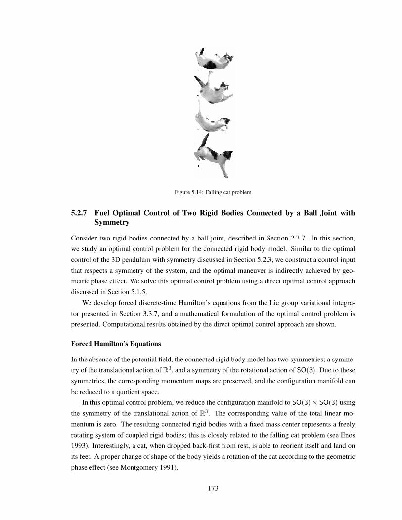
Figure 5.14: Falling cat problem
5.2.7 Fuel Optimal Control of Two Rigid Bodies Connected by a Ball Joint withSymmetry
Consider two rigid bodies connected by a ball joint, described in Section 2.3.7. In this section,
we study an optimal control problem for the connected rigid body model. Similar to the optimal
control of the 3D pendulum with symmetry discussed in Section 5.2.3, we construct a control input
that respects a symmetry of the system, and the optimal maneuver is indirectly achieved by geo-
metric phase effect. We solve this optimal control problem using a direct optimal control approach
discussed in Section 5.1.5.
We develop forced discrete-time Hamilton’s equations from the Lie group variational integra-
tor presented in Section 3.3.7, and a mathematical formulation of the optimal control problem is
presented. Computational results obtained by the direct optimal control approach are shown.
Forced Hamilton’s Equations
In the absence of the potential field, the connected rigid body model has two symmetries; a symme-
try of the translational action of R3, and a symmetry of the rotational action of SO(3). Due to these
symmetries, the corresponding momentum maps are preserved, and the configuration manifold can
be reduced to a quotient space.
In this optimal control problem, we reduce the configuration manifold to SO(3)× SO(3) using
the symmetry of the translational action of R3. The corresponding value of the total linear mo-
mentum is zero. The resulting connected rigid bodies with a fixed mass center represents a freely
rotating system of coupled rigid bodies; this is closely related to the falling cat problem (see Enos
1993). Interestingly, a cat, when dropped back-first from rest, is able to reorient itself and land on
its feet. A proper change of shape of the body yields a rotation of the cat according to the geometric
phase effect (see Montgomery 1991).
173

Similar to the falling cat problem, we assume that an internal control moment is applied at the
joint, that controls the relative attitude between the two rigid bodies. Therefore, the control moment
changes the shape of the system. The total angular momentum is conserved for the controlled
dynamics as the control input is an internal moment of the connected rigid bodies.
The reduced discrete equations of motion on SO(3) × SO(3) can be derived by applying the
discrete Routh reduction procedure discussed in Section 3.1.4. Alternatively, they can be directly
derived from (3.156)–(3.161) by using the fact that the total linear momentum, denoted by p3k ,
is conserved in the absence of a potential: we find an expression for (xk+1 − xk) from (3.159),
and substitute it into (3.156) and (3.158). The resulting forced Hamilton’s equations are given as
follows.
p1k =1h
F1k(Jd1 − αm1d1d
T1 )− (Jd1 − αm1d1d
T1 )F T1k
− βm1
h(RT1kR2kF2kd2d
T1 − d1d
T2 F
T2kRT2kR1k) + β
m1
h(RT1kR2kd2d
T1 − d1d
T2 R
T2kR1k),
(5.96)
p2k =1h
F2k(Jd2 − βm2d2d
T2 )− (Jd2 − βm2d2d
T2 )F T2k
− αm2
h(RT2kR1kF1kd1d
T2 − d2d
T1 F
T1kRT1kR2k) + α
m2
h(RT2kR1kd1d
T2 − d2d
T1 R
T1kR2k),
(5.97)
Rik+1= RikFik , (5.98)
p1k+1= F T1k(p1k − (B1k −B
T1k
)∨) + hRT1k+1uk+1, (5.99)
p2k+1= F T2k(p2k − (B2k −B
T2k
)∨)− hRT2k+1uk+1, (5.100)
where α = m1m1+m2
, β = m2m1+m2
∈ R, and the matrix Bik ∈ R3×3 for i ∈ 1, 2 is defined as
Bik =mi
h(Fik − I)di −αR1k(F1k − I)d1 − βR2k(F2k − I)d2T Rik . (5.101)
Optimal Control Problem
The objective of the optimal control problem is to transfer the connected rigid bodies from a given
initial condition (R10 , R20 ,Ω10 ,Ω20) to a desired terminal condition (Rf1 , Rf2 ,Ω
f1 ,Ω
f2) during a
fixed maneuver time Nh, while minimizing the control effort.
For given: (R10 , R20 ,Ω10 ,Ω20), N, (Rf1 , Rf2 ,Ω
f1 ,Ω
f2)
minuk
Jd =
N∑k=0
h
2uTkWuk
,
such that (R1N , R2N ,Ω1N ,Ω2N ) = (Rf1 , Rf2 ,Ω
f1 ,Ω
f2),
subject to (5.96)–(5.101),
174

where W ∈ R3×3 is a symmetric positive-definite matrix. In particular, we choose attitude maneu-
vers that can be described by rest-to-rest rotations of the entire system while the relative attitude at
the terminal time is the same as that at the initial time.
Numerical Results
The properties of rigid bodies are chosen as
m1 = 1.5kg, J1 =
0.18 0.32 0.320.32 1.88 −0.060.32 −0.06 1.86
kg ·m2, d1 = [−1.08, 0.20, 0.20]m,
m2 = 1kg, J2 =
0.11 −0.18 −0.18−0.18 0.89 −0.04−0.18 −0.04 0.88
kg ·m2, d2 = [0.9, 0.2, 0.2]m.
The desired maneuver is a rest-to-rest rotation about the x axis.
R10 = I, Ω10 = 0, R20 = I, Ω20 = 0,
Rf1 = exp(θe1), Ωf1 = 0, Rf2 = exp(θe1), Ωf
2 = 0,
where the rotation angle is denoted by θ. Two cases are considered, when θ = π2 , and θ = π. The
maneuver time is tf = 4 sec, and the step size is h = 0.01.
We apply the direct optimal control approach discussed in Section 5.1.5. We parameterize each
component of the control input at 7 discrete points, and the control inputs are reconstructed by cubic
spline interpolation. The resulting 21 control input parameters are optimized using a sequential
quadratic programming method to satisfy the terminal boundary conditions while minimizing the
cost function. The terminal angular velocity constraint for the second body is not imposed since it is
satisfied automatically by the other three constraints due to the total angular momentum preservation
property. By formulating the optimization process this way, we eliminate a source of numerical ill-
conditioning. This is similar to the modified computational approach for the indirect optimal control
discussed in Section 5.2.3 for the optimal control of the 3D pendulum with symmetry.
The optimized maneuver, the angular velocity, the control input trajectories, and the total angu-
lar momentum in the reference frame are shown in Figure 5.15 and Figure 5.16. The optimal cost
and the violation of the terminal boundary conditions are Jd = 0.154, 1.19×10⁻⁸, and Jd = 0.574,
2.48 × 10⁻⁸, respectively for θ = π2 , and θ = π. Throughout this complicated maneuver, the total
angular momentum is zero, and the rotation about the e1 axis is purely caused by the geometric
phase effect. This also demonstrates the advantages of the computational geometric optimal control
approach. The Lie group variational integrator computes the weak geometric phase effect accu-
rately, so that the iterations converge to a nontrivial optimal maneuver of the coupled rigid bodies.
175

(a) Optimal maneuver
0 1 2 3 4−2
0
2
0 1 2 3 4−1
0
1
Ω1
0 1 2 3 4−2
0
2
t
(b) Angular velocity Ω1
0 1 2 3 4−5
0
5
0 1 2 3 4−2
0
2
Ω2
0 1 2 3 4−2
0
2
t
(c) Angular velocity Ω2
0 1 2 3 4−0.1
0
0.1
0 1 2 3 4−0.5
0
0.5
u
0 1 2 3 4−0.5
0
0.5
t
(d) Control input u
0 1 2 3 4
−0.50
0.5
x 10−10
0 1 2 3 4
−0.50
0.5
x 10−10
πT
0 1 2 3 4
−0.50
0.5
x 10−10
t
(e) Total angular momentum
Figure 5.15: Optimal control of two connected rigid bodies (θ = π/2)
176

(a) Optimal maneuver
0 1 2 3 4−5
0
5
0 1 2 3 4−2
0
2
Ω1
0 1 2 3 4−5
0
5
t
(b) Angular velocity Ω1
0 1 2 3 4−5
0
5
0 1 2 3 4−5
0
5
Ω2
0 1 2 3 4−5
0
5
t
(c) Angular velocity Ω2
0 1 2 3 4−0.2
0
0.2
0 1 2 3 4−1
0
1
u
0 1 2 3 4−1
0
1
t
(d) Control input u
0 1 2 3 4
−0.50
0.5
x 10−10
0 1 2 3 4
−0.50
0.5
x 10−10
πT
0 1 2 3 4
−0.50
0.5
x 10−10
t
(e) Total angular momentum
Figure 5.16: Optimal control of two connected rigid bodies (θ = π)
177

5.3 Conclusions
In this chapter, a computational geometric approach for an optimal control problem of rigid bodies
has been discussed. The essential idea is formulating a discrete-time optimal control problem using
a Lie group variational integrator, and applying standard optimal control approaches, such as an
indirect optimal control approach or a direct optimal control approach to the discrete-time equations
of motion. This method is in contrast to the usual optimal control approach, where the discretization
appears in the last stage to find the optimal control inputs numerically.
The computational geometric optimal control approach has substantial advantages in terms of
preserving the geometric properties of the optimality conditions. As discussed in Chapter 3, a
discrete flow of a Lie group variational integrator has desirable geometric properties, and it is more
reliable over long time periods. The computational geometric optimal control approach inherits the
desirable properties of the Lie group variational integrator. In necessary conditions for optimality,
multiplier equations can be considered as a dual system of linearized equations of motion. Since the
linearized flow of a Lagrangian/Hamiltonian system is symplectic, the multiplier equations also have
geometric properties. The discrete-time necessary conditions, presented in Section 5.1.3, preserve
the geometric properties of the optimality conditions, as they are derived from a symplectic discrete
flow.
The computational geometric optimal control approach allows us to find the optimal control
inputs efficiently. In indirect optimal control, the shooting method may be prone to numerical ill-
conditioning, since a small change in the initial multipliers can cause highly nonlinear behavior of
the terminal conditions. It is difficult to compute the Jacobian matrix for Newton iterations accu-
rately, and consequently, the numerical error may not converge to machine precision. However,
as shown in Figure 5.1(c), 5.2(c), 5.5(e), and 5.6(e), the computational geometric optimal con-
trol approach exhibits excellent numerical convergence properties. This is because the proposed
computational algorithms are geometrically exact and numerically accurate. There is no numerical
dissipation caused by the numerical algorithm, and therefore, we obtain more accurate sensitivities
along the optimal solution.
Another advantage of computational geometric optimal control of rigid bodies is that the method
is directly developed on a Lie group. There is no ambiguity or singularity in representing the config-
uration of rigid bodies globally. For example, we can study large-angle optimal attitude maneuvers
as presented in Section 5.2.1, Section 5.2.6, and Section 5.2.7, and we can consider nontrivial cou-
pling effects between the translational maneuver and the rotational maneuver of a rigid body, as
presented in Section 5.2.4.
178

CHAPTER 6
CONCLUSIONS
6.1 Conclusions
In this dissertation, computational geometric mechanics and optimal control have been developed
for dynamic systems evolving on a Lie group, with applications to rigid body dynamics. Theoreti-
cal results are presented both for continuous-time dynamic systems and for discrete-time dynamic
systems in parallel, and they are applied to several nontrivial rigid body dynamics.
Geometric Mechanicsfor Rigid Bodies on a Lie Group
Generalized Euler-Poincare equation on G
Euler-Lagrange equations on (S2)n
Computational Geometric Mechanicsfor Rigid Bodies on a Lie Group
Lie group variational integrator on G
Homogeneous variational integrator on (S2)n
Planar pendulum, 3D pendulum, 3D pendulum with an internal degree of freedom, 3D pendulum on a cart,Single rigid body, Full body problem, Two rigid bodies connected by a ball joint
Double Spherical Pendulum, n-body problem on a sphere, Pure bending of elastic rod,Spatial array of magnetic dipoles, Molecular dynamics on a sphere
Geometric Optimal Controlfor Rigid Bodies on a Lie Group
Necessary conditions for optimality on G
Computational Geometric Optimal Controlfor Rigid Bodies on a Lie Group
Discrete-time necessary conditions for optimality on GDirect optimal control approach
Fuel optimal attitude control of a spacecraft, Time optimal attitude control of a free rigid body,Fuel optimal attitude control of a 3D pendulum with symmetry, Fuel optimal control of a rigid body,
Combinatorial optimal control of spacecraft formation reconfiguration,Fuel optimal control of a 3D pendulum on a cart,
Fuel optimal control of two rigid bodies connected by a ball joint
The continuous-time equations of motion for dynamic system on a Lie group are presented in
Chapter 2. They can be considered as either a generalized form of Euler-Poincare equations or a
left-trivialized form of Euler-Lagrange equations on a manifold. The tangent bundle of a Lie group
TG is identified with G × g by the left trivialization, and the equations of motion are expressed in
terms of Lie group elements and Lie algebra elements. Even if the Lagrangian is not left invariant,
this approach is still desirable: since a Lie algebra is a linear vector space at the fixed identity
179

element, there is no need to deal with covariant derivatives or Christoffel symbols. The resulting
equations of motion for multiple rigid body systems are more compact and concise.
Geometric numerical integrators, referred to as Lie group variational integrators, are developed
for dynamic systems with a Lie group configuration manifold. The method presented in this disser-
tation represents the first time that the Lie group approach has been explicitly adopted in the context
of variational integrators for an arbitrary Lie group. They provide a systematic way to develop
a class of geometric numerical integrators that preserve the geometric properties of the dynamics
as well as the Lie group structure. Numerical simulations show that it is critical to preserve both
the symplectic property of the dynamics and the structure of the Lie group. The Lie group varia-
tional integrators have substantial computational advantages compared to other geometric integra-
tors that preserve either none or one of these properties. They are more efficient than considering
the Lie group structure as a nonlinear algebraic constraint to be satisfied at each time step. The
Lie group variational integrator is extended to mechanical systems evolving on a product of two-
spheres, which provides an overall framework to develop variational integrators on a homogeneous
manifold.
Geometric optimal control, as presented in this dissertation, is used to treat optimal control
problems for dynamic systems on a Lie group. This is distinguished from the existing optimal
control theories developed for kinematics equations on a Lie group. In Chapter 4, an intrinsic form
of necessary conditions for optimality is developed. They are applied to a wide class of dynamic
systems on a Lie group, and they are more compact than optimality conditions expressed in terms
of local coordinates.
Computational geometric optimal control formulates a discrete-time optimal control problem
based on geometric numerical integrators. This is in contrast to other optimal control approaches
where a discretization appears at the terminal stage in solving optimality conditions numerically.
The computational geometric optimal control preserves the geometric structure of the optimal con-
trol problem as well as the geometric properties of the dynamics. It turns out that the approach also
allow us to find the optimal trajectory more efficiently since there is no numerical dissipation in the
discrete-time numerical flow. This is applied to several optimal control problems for rigid bodies.
In summary, this dissertation develops computational geometric mechanics and computational
geometric optimal control approaches for dynamic systems on a Lie group. The essential idea is to
derive a computational algorithm from a discrete analogue of the underlying fundamental principles
so that the physical properties are preserved naturally. They are applied to several nontrivial rigid
body dynamics.
6.2 Future Work
This dissertation has a broad scope; it combines system and control theory in engineering and dif-
ferential geometry in applied mathematics. The resulting computational geometric methods have
broad potential impact on numerous scientific and engineering problems varying from formation re-
180

configuration in aerospace engineering to molecular dynamics simulations in chemistry. Therefore,
the results in this dissertation can be extended in various directions.
Generalized Lie Group Variational Integrator. The variational integrators have been extended in
various ways. For example, a variational integrator for a Lagrangian system with a degenerate La-
grangian has been developed by Rowley and Marsden (2002) with application to point vortices, and
multisymplectic variational integrators have been developed for Hamiltonian continuum mechan-
ics (see Marsden et al. 2001). Asynchronous variational integrators in the work by Lew et al. (2003)
consider variational integrators with varying step size. Generalized variational integrators are de-
veloped for nonsmooth systems by Fetecau et al. (2003), and for nonholonomic systems by Cortes
and Martınez (2001).
The presented Lie group variational integrators can be extended in similar ways to obtain gen-
eralized Lie group variational integrators for various types of mechanical systems. In particular,
it would be interesting to develop a multiple time-scale Lie group variational integrator for highly
oscillatory systems. This is motivated by scientific and engineering problems from molecular dy-
namics, astrophysics, structural dynamics, and nonlinear wave equations.
Discrete-time Geometric Control Systems on a Lie Group. Geometric mechanics provides funda-
mental insights into mechanical systems and yields new approaches in control system design. For
example, the method of controlled Lagrangian is a constructive technique for stabilizing mechanical
systems, where control inputs are obtained from a Lagrangian system with a modified Lagrangian.
This approach originated by Bloch et al. (1992) has been extended in various ways (see, for example,
Bloch et al. 2000, 2001; Zenkov et al. 2000, 2002, and references therein).
In particular, a discrete-time theory of controlled Lagrangian systems was developed for vari-
ational integrators by Bloch et al. (2005, 2006), and applied to the feedback stabilization of the
unstable inverted equilibrium of a planar pendulum on a cart. It would be natural to combine the
techniques of the controlled Lagrangian method and the Lie group variational integrators developed
in this dissertation to obtain a discrete-time geometric control approach for mechanical systems on
a Lie group.
Uncertainty Propagation and Estimation on a Lie Group. A mathematical model of a dynamic
system may not capture all of the dynamic characteristics of the system exactly. It always includes
approximations, simplifications, or system identification errors. Therefore, uncertainty propagation
and estimation provide important information for many scientific and engineering problems. How-
ever, it is challenging in the sense that uncertainty propagation for a general nonlinear system is
expressed as a partial differential equation. The standard linearization approach is only applicable
to a system with frequent measurements.
A deterministic attitude estimation scheme has been developed by Lee et al. (2006b, 2007h);
Sanyal et al. (2008) using the Lie group variational integrator; limitations of the linearization ap-
proach for uncertainty propagation of attitude dynamics have been presented in Lee et al. (2007a).
181

Recently, a global uncertainty propagation scheme for the attitude dynamics of a rigid body is devel-
oped by Lee et al. (2008b). This approach is based on the symplectic property of the attitude dynam-
ics and noncommutative harmonic analysis on a Lie group: the symplectic property of Hamiltonian
systems imposes a fundamental limit on the uncertainty propagation (see Hsiao and Scheeres. 2007;
Scheeres et al. 2005), which yields a particle based uncertainty propagation method. The propa-
gated probability density function is expressed in term of noncommutative harmonic analysis (see,
for example Biedenharn and Louck 1981; Chirikjian and Kyatkin 2001; Sugiura 1990).
Application to Large Scale Full n-body Problems. The full n body problem studies the motion
of n interacting bodies modeled as rigid bodies with arbitrary shapes. Since the motion of each
rigid body is described by its translation and rotation with respect to a given reference frame, the
configuration space for the full n body problem is SE(3)n. This is particularly important for various
physical systems where the mutual interaction depends on the relative attitude as well as the relative
position. For example, the mutual gravitational forces and moments in binary asteroids vary with
the rotation of each body, and the electrostatic forces between charged molecules depend on their
electric pole directions.
The computational accuracy and efficiency of Lie group variational integrators has been illus-
trated by a full two body problem. Since the computational superiority of the Lie group variational
integrators increases as the complexity of the system or the simulation time increases, they can be
applied to challenging full n body problems such as simulations of the asteroid belt or molecular
dynamics, using powerful parallel computing resources.
Applications to Multibody Systems. Multibody systems appear in advanced mechanical systems in
the area of automobiles, aerospace, robotics, and power plants. For example, solar panel deployment
in satellites, bipedal robots, cooperative multiple vehicles, or flexible bodies are often analyzed as
multibody systems.
Lie group variational integrators can be applied to any multibody system whose configuration
manifold is expressed as a product of Lie groups, Euclidean spaces or two-spheres, thereby generat-
ing structure-preserving geometric numerical integrators for the multibody system. The continuous-
time counterpart of this development provides a remarkably compact form for global equations of
motion. These give both an efficient computational approach and a powerful analysis tool for multi-
body systems.
In particular, it would be be interesting to study optimal maneuvers of a large space tether,
which controls its orbit by changing its shape. This requires significantly less expensive propulsion
than spacecraft using rocket engines. The elastic rod model presented in Section 3.4.4, and the
underactuated optimal control approach discussed in Section 5.2.3 and Section 5.2.7 might serve as
a basis for this research.
182

APPENDIX
183

APPENDIX A
PROPERTIES AND PROOFS
A.1 Properties of the hat Map
The hat map · : R3 → so(3) is defined as
x =
0 −x3 x2
x3 0 −x1
−x2 x1 0
(A.1)
for x = [x1;x2;x3] ∈ R3. This identifies the Lie algebra so(3) with R3 using the vector cross
product in R3.
Several properties of the hat map are summarized as follows.
xy = x× y = −y × x = −yx, (A.2)
xT x = (xTx)I − xxT , (A.3)
xyx = −(yTx)x, (A.4)
−12
tr[xy] = xT y, (A.5)
x× y = xy − yx = yxT − xyT , (A.6)
tr[xA] =12
tr[x(A−AT )
], (A.7)
Ax = x
(12
tr[A] I −A)
+(
12
tr[A] I −A)T
x, (A.8)
xA+AT x = (tr[A] I3×3 −Ax)∧. (A.9)
for any x, y ∈ R3, A ∈ R3×3.
184

A.2 Inertia Matrix of a Rigid Body
Consider a rigid body B. We define a body fixed frame. Let ρ ∈ R3 be the vector from the origin of
the body fixed frame to a mass element of the rigid body.
The inertia matrix J ∈ R3×3 of the rigid body is given by
J =∫BρT ρ dm(ρ) =
∫B
y2 + z2 −xy −zx−xy z2 + x2 −yz−zx −yz x2 + y2
dm(ρ), (A.10)
where x, y, z ∈ R are the coordinates of the vector ρ, i.e. ρ = [x; y; z]. We define a nonstandard
inertia matrix Jd ∈ R3×3 as
Jd =∫BρρT dm(ρ) =
∫B
x2 xy zx
xy y2 yz
zx yz z2
dm(ρ). (A.11)
From the coordinate expressions, it is clear that the standard inertia matrix J and the nonstandard
inertia matrix Jd represent the second order mass distributions of the rigid body. Using the property,
ρT ρ = (ρTρ)I3×3 − ρρT , it can be shown that
Jd =12
tr[J ] I3×3 − J, J = tr[Jd] I3×3 − Jd. (A.12)
In Section 2.3.2, we show that the rotational kinetic energy of the rigid body, when it rotates
about the origin with an angular velocity Ω ∈ R3, can be written as
T =12
ΩTJΩ =12
tr[ΩJdΩT
]. (A.13)
Furthermore, the following equation is satisfied for any Ω ∈ R3.
JΩ = ΩJd + JdΩ. (A.14)
A proof for (A.14) is as follows. Let Ω = [Ω1,Ω2,Ω3] for any Ω1,Ω2,Ω3 ∈ R. By substitution
and rearrangement, it is straightforward to show that both the left hand side expression and the right
hand side expression of (A.14) are equal to (Jyy + Jzz)Ω1 − JxyΩ2 − JzxΩ3
−JxyΩ1 + (Jzz + Jxx)Ω2 − JyzΩ3
−JzxΩ1 − JyzΩ2 + (Jxx + Jyy)Ω3
∧
,
where Jxy =∫B xy dm(ρ) ∈ R, and other terms are defined similarly.
185

A.3 Lagrangian-Routh Reduction of the 3D Pendulum
The 3D pendulum is a rigid body supported by a frictionless pivot point acting under a gravitational
potential (see Section 2.3.2). The configuration manifold is SO(3). The Lagrangian of the 3D
pendulum has a symmetry: it is invariant under an action of H = SO(2) ' S1 given by Φ :S1 × SO(3)→ SO(3)
Φ(θ,R) = expSO(3)(θe3)R, (A.15)
which represents the rotation of the 3D pendulum about the gravity direction e3. As a result, the
configuration manifold can be reduced to the quotient space SO(3)/SO(2) ' S2.
Here, we summarize the Lagrange-Routh reduction and reconstruction procedure to obtain the
reduced equations of motion of the 3D pendulum on S2 (see Marsden et al. 2000). This reduc-
tion procedure is interesting and challenging, since the projection proj : SO(3) → S2 given by
proj(R) = RT e3 = Υ together with the symmetry action has a nontrivial principal bundle struc-
ture. In other words, the angle of the rotation about the vertical axis is not a global cyclic variable.
A.3.1 Reduction
The procedure for Lagrange-Routh reduction is as follows. We find expressions for the mechanical
connection, from which a Routhian is defined. The Routhian satisfies the Lagrange-d’Alembert
principle with a magnetic two-form, which yields the reduced Euler-Lagrange equations.
Routhian We identify the Lie algebra of S1 with R. At (2.71), the momentum map of the 3D
pendulum JL : SO(3)× so(3)→ R∗ is given by
JL(R, Ω) = eT3 RJΩ. (A.16)
The locked inertia tensor I(R) : R→ R∗ is defined as
〈I(R)%, ζ〉 = 〈〈%SO(3), ζSO(3)〉〉
for %, ζ ∈ R. Substituting the expression for the infinitesimal generator ζSO(3) = ζRT e3, %SO(3) =
%RT e3 given by (3.84), we obtain
%ζI(R) = %ζeT3 RJRT e3.
Thus, the locked inertia tensor is given by I(R) = eT3 RJRT e3. The mechanical connection A :
SO(3)× so(3)→ R is given by
A(R, Ω) = I−1(R)JL(R, Ω) =eT3 RJΩ
eT3 RJRT e3
. (A.17)
Using the mechanical connection, we decompose the tangent space into a vertical space and a
186

horizontal space as follows. For a given (R, Ω) ∈ TSO(3), the horizontal part and the vertical part
are obtained by
ver(R, Ω) = (A(R, Ω))SO(3)(R) =eT3 RJΩ
eT3 RJRT e3
RT e3 =Υ · JΩΥ · JΥ
Υ,
hor(R, Ω) = Ω− ver(R, Ω) =(
Ω− RT e3eT3 RJ
eT3 RJRT e3
Ω)∧
=(
Ω− ΥΥTJ
Υ · JΥΩ)∧
.
Since Υ = RT e3 = −ΩRT e3 = Υ× Ω, we obtain
Υ×Υ = (Υ× Ω)×Υ = (ΥTΥ)Ω− (ΥTΩ)Υ = Ω−ΥΥTΩ.
Using this expression, the horizontal part of Ω can be written in terms of Υ as
Ωhor = Υ×Υ− JΥ · (Υ×Υ)Υ · JΥ
Υ = Υ×Υ− bΥ
for b = JΥ·(Υ×Υ)Υ·JΥ . For the given value of the momentum map ν ∈ R∗, the Routhian of the 3D
pendulum is given by
Rν(Υ, Υ) =12
Ωhor · JΩhor −mgΥ · ρ− 12
ν2
Υ · JΥ
=12
(Υ×Υ) · J(Υ×Υ)− 12
(b2 + γ2)(Υ · JΥ) +mgΥ · ρ, (A.18)
where γ = νΥ·JΥ .
Variation of the Routhian The Routhian satisfies the variational Lagrange-d’Alembert principle.
The infinitesimal variation for Υ ∈ S2 is chosen as:
δΥ = Υ× η, (A.19)
δΥ = Υ× η + Υ× η. (A.20)
Here we assume that η ·Υ = 0, since the component of η parallel to Υ has no effect on δΥ. These
expressions are essential for developing the reduced equations of motion.
Using (A.19), (A.20), and the properties Υ · Υ = 0, Υ · η = 0, the variation of the Routhian is
given by
δRν = η · J(Υ×Υ− bΥ)
− η ·Υ×[−Υ× J(Υ×Υ) + (b2 + λ2)JΥ− bJ(Υ×Υ) + b(Υ× JΥ) +mgρ
].
(A.21)
187

Magnetic two-form From the given mechanical connection A and a value of the momentum map
ν ∈ R∗, define a one-form Aν on SO(3)× so(3) by
Aν(R) · (R, Ω) =⟨ν,A(R, Ω)
⟩= ν
eT3 RJΩeT3 RJR
T e3.
The magnetic two-form βν is the exterior derivative of Aν , which can be obtained by using the
identity
dAν(X,Y ) = X[Aν(Y )]− Y [Aν(X)]−Aν([X,Y ])
for X = Rη, Y = Rξ ∈ TRSO(3), where X[Aν(Y )] denotes the Lie derivative of Aν(Y ) along
X (see Marsden and Ratiu 1999). The first term of the above equation is obtained as
X[Aν(Y )] =d
dε
∣∣∣∣ε=0
Aν(Y )R=R exp εη
=ν
(eT3 RJRT e3)2
[eT3 RηJξ(e
T3 RJR
T e3) + 2eT3 RJξ(eT3 RJηR
T e3)]
=ν
(eT3 RJRT e3)2
[−Jξ · (η ×RT e3)(eT3 RJR
T e3) + 2(ξ · JRT e3)(JRT e3 · (η ×RT e3))].
Similarly, we find expressions for Y [Aν(X)]. The Lie bracket is given by [X,Y ] = Rη × ξ.
Therefore, we obtain
dAν(X,Y ) = − ν
(eT3 RJRT e3)
[Jξ · (η ×RT e3)− Jη · (ξ ×RT e3) + (η × ξ) · JRT e3
]− ν
(eT3 RJRT e3)2
[−2(ξ · JRT e3)(JRT e3 · (η ×RT e3)) + 2(η · JRT e3)(JRT e3 · (ξ ×RT e3))
].
Substituting Υ = RT e3 into this, the magnetic two form is given by
βν(Υ× η,Υ× ξ) = − ν
(Υ · JΥ)[Jξ · (η ×Υ)− Jη · (ξ ×Υ) + (η × ξ) · JΥ]
− ν
(Υ · JΥ)2[−2(ξ · JΥ)(JΥ · (η ×Υ)) + 2(η · JΥ)(JΥ · (ξ ×Υ))] .
Since (a · x)(b · y)− (a · y)(b · x) = (a× b) · (x× y) for any a, b, x, y ∈ R3, the last two terms of
the above equation are reduced to
−2(ξ · JΥ)(JΥ · (η ×Υ)) + 2(η · JΥ)(JΥ · (ξ ×Υ))
= −2(ξ · JΥ)(η · (Υ× JΥ)) + 2(η · JΥ)(ξ · (Υ× JΥ))
= 2(JΥ× (Υ× JΥ)) · (η × ξ)
= 2‖JΥ‖2 Υ− (Υ · JΥ)JΥ
· (η × ξ).
188

Thus, we obtain
βν(Υ× η,Υ× ξ)
= − ν
(Υ · JΥ)2
[(Υ · JΥ) Υ · (Jξ × η)−Υ · (Jη × ξ)− JΥ · (η × ξ)+ 2 ‖JΥ‖2 Υ · (η × ξ)
].
Using the identity, Υ · (Jξ × η) + Υ · (ξ × Jη) + JΥ · (ξ × η) = tr[J ] Υ · (ξ × η), the magnetic
two form βν is given by
βν(Υ× η,Υ× ξ) = − ν
(Υ · JΥ)2
[−(Υ · JΥ)tr[J ] + 2 ‖JΥ‖2
]Υ · (η × ξ). (A.22)
Since Υ = Υ×Ω, and Υ · (ω × η) = η · (Υ× ω) = η · Υ, the interior product of the magnetic
two-form is given by
iΥβν(δΥ) = βν(Υ× Ω,Υ× η) = λ
tr[J ]− 2
‖JΥ‖2
Υ · JΥ
Υ · η, (A.23)
where λ = νΥ·JΥ .
Lagrange-d’Alembert Principle The Routhian satisfies the Lagrange-d’Alembert principle with
the magnetic term, given by
δ
∫ T
0Rν(Υ, Υ)dt =
∫ T
0iΥβν(δΥ)dt. (A.24)
Substituting (A.21) and (A.23) into (A.24), and integrating by parts, we obtain
−∫ T
0η ·[J(Υ×Υ− bΥ− bΥ) + Υ×X + cΥ
]dt = 0, (A.25)
where
X = −Υ× J(Υ×Υ) + (b2 + λ2)JΥ− bJ(Υ×Υ) + b(Υ× JΥ) +mgρ, (A.26)
and c is given by (2.74):
c = Υ
tr[J ]− 2
‖JΥ‖2
Υ · JΥ
.
Since (A.25) is satisfied for all η with Υ · η = 0, we obtain
J(Υ×Υ− bΥ− bΥ) + Υ×X + cΥ = aΥ, (A.27)
for a constant a ∈ R. This is the reduced equation of motion. However, this equation has an
ambiguity since the value of the constant a is unknown; this equation is implicit for Υ since the
term b is expressed in terms of Υ. The next step is to determine expressions for a and b using the
definition of b and several vector identities.
189

We first find an expression for the constant a in terms of Υ, Υ. Taking the dot product of (A.27)
with Υ, we obtain
Υ · J(Υ×Υ− bΥ− bΥ) = a. (A.28)
From the definition of b, we can show the following identity: Υ·J(Υ×Υ−bΥ) = 0. Differentiating
this with time, and substituting into (A.28), we find an expression for the constant a in terms of Υ, Υas
a = −Υ · J(Υ×Υ− bΥ). (A.29)
Substituting (A.29) into (A.27), and taking the dot product of the result with Υ, we obtain an ex-
pression for b in terms of Υ, Υ as
b = Υ · J−1
Υ×X + cΥ + (Υ · J(Υ×Υ− bΥ))Υ. (A.30)
Substituting (A.30) into (A.27), and using the vector identity Y −(Υ·Y )Υ = (Υ·Υ)Y −(Υ·Y )Υ =−Υ× (Υ× Y ) for any Y ∈ R3, we obtain the following form for the reduced equation of motion
Υ×Υ− bΥ−Υ×[Υ× J−1
Υ×X + cΥ + (Υ · J(Υ×Υ− bΥ))Υ
]= 0.
Now, we simplify this equation. The above expression is equivalent to the following equation
Υ×[Υ×Υ− bΥ−Υ×
[Υ× J−1
Υ×X + cΥ + (Υ · J(Υ×Υ− bΥ))Υ
]]= 0. (A.31)
Since Υ · Υ = −‖Υ‖2, the first term is given by
Υ× (Υ×Υ) = (Υ ·Υ)Υ− (Υ · Υ)Υ = Υ + ‖Υ‖2Υ.
Using the property Υ× (Υ× (Υ× Y )) = −(Υ ·Υ)Υ× Y = −Υ× Y for Y ∈ R3, the third term
of (A.31) can be simplified.
Reduced Euler-Lagrange Equations Substituting (A.26) and rearranging, the reduced Euler-Lagrange
equations for the 3D pendulum on S2 are given by
Υ = −‖Υ‖2Υ + Υ× Σ, (A.32)
where Σ = bΥ + J−1[(J(Υ×Υ)− bJΥ)× ((Υ×Υ)− bΥ) + λ2JΥ×Υ−mgΥ× ρ− cΥ
],
which recovers (2.72)–(2.74).
A.3.2 Reconstruction
For a given integral curve of the reduced equation Υ(t) : [0, T ] → S2, the reconstruction is to find
the corresponding curve R(t) : [0, T ]→ SO(3) that is projected to the given curve and satisfies the
Euler-Lagrange equations.
190
We first choose a curve R(t) ∈ SO(3) that is projected into the reduced curve, i.e. proj(R(t)) =Υ(t). Then, the reconstructed curve can be written asR(t) = Φθ(t)(R(t)) for some θ(t) ∈ S1. Con-
servation of the momentum map yields the following reconstruction equation for θ(t) (see Marsden
et al. 2000).
θ(t)−1θ(t) = I−1(R(t))ν −A( ˙R(t)).
If we choose R(t) as the horizontal lift, the last term vanishes as the horizontal space is annihilated
by the mechanical connection. Since the symmetry group is abelian, the solution reduces to a
quadrature as
θ(t) = θ(0) expSO(2)
[∫ t
0I−1(R(s))ν ds
].
In summary, the reconstruction procedure is as follows.
(i) Horizontally lift Υ(t) to obtain Rhor(t) by integrating the following equation with Rhor(0) =R(0)
Rhor(t) = Rhor(t)Ωhor(t), (A.33)
where
Ωhor(t) = Υ(t)×Υ(t)− JΥ(t) · (Υ(t)×Υ(t))Υ(t) · JΥ(t)
Υ(t). (A.34)
(ii) Determine θdyn(t) ∈ S by the following equation
θdyn(t) =∫ t
0
ν
Υ(s) · JΥ(s)ds. (A.35)
(iii) Reconstruct the curve in SO(3) as
R(t) = θdyn(t) ·Rhor(t) = exp[θdyn(t)e3]Rhor(t). (A.36)
A.3.3 Geometric Phase
Suppose that the integral curve in S2 is a closed curve, i.e. Υ(0) = Υ(T ). Since Rhor(0) = R(0)and Rhor(T ) are in the same fiber, Rhor(T ) can be written as
Rhor(T ) = θgeo(T ) ·R(0),
for θgeo(T ) ∈ S1. From the reconstruction equation (A.36), we obtain
R(T ) = θdyn(T ) · θgeo(T ) ·R(0),
191

where θdyn(T ) ∈ S1 and θgeo(T ) ∈ S1 are referred to as the dynamic phase and the geometric
phase, respectively. If the value of the momentum map is zero, then the dynamic phase is also zero
from (A.35), and the attitude is changed only by the geometric phase effect.
It can be shown that the geometric phase is the negative of the integral of the magnetic two-form
on the area enclosed by the integral curve Υ(t)
θgeo(T ) =∫S
2 ‖JΥ(t)‖2 − tr[J ] (Υ(t) · JΥ(t))(Υ(t) · JΥ(t))2
dA, (A.37)
where S is an area in S2 with Υ(t) as a boundary.
192

A.4 Commutativity of the Variation and the Time Derivative
Here, we show the commutativity of the variation operation and the time derivative for ξ = g−1g ∈g, i.e, d
dt(δξ) = δ( ddtξ). We give a proof for a matrix Lie group; an extension to general Lie groups
can be developed using the results presented in Bloch et al. (1996).
Recall that for a curve g in G, we define ξ = g−1g. The variation is chosen as gε = g exp εη for
η ∈ g so that the infinitesimal variation is given by δg = gη. Thus, η = g−1δg. We first find the
expression for δξ in (2.5) (see Marsden and Ratiu 1999)
δξ =d
dε
∣∣∣∣ε=0
((gε)−1dg
ε
dt
)= −(g−1δgg−1)g + g−1d
2gε
dεdt
∣∣∣∣ε=0
= −ηξ + g−1d2gε
dεdt
∣∣∣∣ε=0
. (A.38)
But, ddtη is given by
η =d
dt
(g−1dg
dε
) ∣∣∣∣ε=0
= −(g−1gg−1)δg + g−1d2gε
dtdε
∣∣∣∣ε=0
= −ξη + g−1d2gε
dtdε
∣∣∣∣ε=0
. (A.39)
Since the partial derivatives commute for smooth maps, the difference is given by δξ−η = ξη−ηξ =[ξ, η], which yields
δξ = η + [ξ, η]. (A.40)
This gives (2.5).
Now we show that ddt(δξ) = δ( ddtξ). The time derivative of δξ is given by
d
dt(δξ) = η + [ξ, η] + [ξ, η]. (A.41)
Now, we find an expression for the variation of ξ.
δ(d
dtξ) =
d
dε
∣∣∣∣ε=0
d
dt
((gε)−1dg
ε
dt
)=
d
dε
∣∣∣∣ε=0
−(
(gε)−1dgε
dt(gε)−1
)dgε
dt+ (gε)−1d
2gε
dt2
= (g−1δgg−1)gg−1g − g−1d
2gε
dεdt
∣∣∣∣ε=0
g−1g + g−1g(g−1δgg−1)g − (g−1gg−1)d2gε
dεdt
∣∣∣∣ε=0
− (g−1δgg−1)g + g−1 d3gε
dεdt2
∣∣∣∣ε=0
Since g−1δg = η and g−1g = ξ, this reduces to
δ(d
dtξ) = ηξξ − g−1d
2gε
dεdt
∣∣∣∣ε=0
ξ + ξηξ − ξg−1d2gε
dεdt
∣∣∣∣ε=0
− ηg−1g + g−1 d3gε
dεdt2
∣∣∣∣ε=0
. (A.42)
193

From (A.39), we have g−1 d2gε
dεdt
∣∣ε=0
= η + ξη. Therefore, we obtain
g−1 d3gε
dεdt2
∣∣∣∣ε=0
= g−1 d
dt(gη + gξη) = (ξη + η + ξξη + ξη + ξη).
Since g = gξ, we have g−1g = ξξ + ξ. Substituting these into (A.42), we obtain
δ(d
dtξ) = ηξξ − (η + ξη)ξ + ξηξ − ξ(η + ξη)− η(ξξ + ξ) + (ξη + η + ξξη + ξη + ξη)
= η + (ξη − ηξ) + (ξη − ηξ),
which is equal to (A.41). Therefore, ddt(δξ) = δ( ddtξ).
194

A.5 Proof of Corollary 5.1
Corollary 5.1 shows the forced discrete-time Euler-Lagrange equations and the discrete-time Hamil-
ton’s equations for a special form of the discrete Lagrangian and the generalized forces. Suppose
that the discrete Lagrangian and the generalized forces are given (5.7) and (5.8):
Ld(gk, fk) = Td(fk)− (1− c)hU(gk)− chU(gkfk),
u−dk = (1− c)huk, u+dk
= chuk+1,
where the constant c is a free parameter lies in the interval [0, 1]. We develop the corresponding
discrete-time equations of motion from Proposition 5.1.
Derivatives of the Discrete Lagrangian We first find expressions for the derivatives of the discrete
Lagrangian. The derivative of the discrete Lagrangian with respect to fk is given by
DfkLdk · δfk = DfkTdk · δfk − chDU(gkfk) · TfkLgkδfk= DfkTdk · (TeLfk TfkLf−1
kδfk)− chDU(gkfk) · (TfkLgk TeLfk TfkLf−1
kδfk)
=⟨T∗eLfk ·DfkTdk − chT
∗eLgkfk ·DU(gkfk), TfkLf−1
kδfk
⟩.
Since the force due to the potential is defined as M(g) = −T∗eLg ·DU(g), we obtain
T∗eLfk ·DfkLdk = T∗eLfk ·DfkTdk + chM(gk+1). (A.43)
From the definition of the Ad operator, for any α ∈ g∗ and η ∈ g, we have⟨α, Adf−1η
⟩=⟨α, TfLf−1 TeRfη
⟩=⟨α, Tf−1Rf TeLf−1η
⟩=⟨T∗eRf T∗fLf−1α, η
⟩=⟨T∗eLf−1 T∗f−1Rfα, η
⟩=⟨
Ad∗f−1α, η⟩
Thus, Ad∗f−1α = T∗eLf−1 T∗f−1Rf = T∗eRf T∗fLf−1 . Using this, we obtain
Ad∗f−1k
· (T∗eLfk ·DfkLdk) = Ad∗f−1k
· (T∗eLfk ·DfkTdk)
− chT∗eRfk T∗fkLf−1k
(T∗eLgkfk ·DU(gkfk))
= Ad∗f−1k
· (T∗eLfk ·DfkTdk)− chT∗eRfk T∗fkLgk ·DU(gkfk)).
(A.44)
The derivative of the discrete Lagrangian with respect to gk is given by
DgkLdk · δgk = −chDU(gk) · δgk − (1− c)hDU(gkfk) · TRfkδgk
= −chDU(gk) · (TeLgk TgkLg−1kδgk)
− (1− c)hDU(gkfk) · (TgkRfk TeLgk TgkLg−1kδgk)
195

= −⟨chT∗eLgk ·DU(gk) + (1− c)hT∗eLgk T∗gkRfk ·DU(gkfk), TgkLg−1
kδgk
⟩Thus, we obtain
T∗eLgkDgkLdk = (1− c)hM(gk)− chT∗eLgk T∗gkRfk ·DU(gkfk). (A.45)
Forced Discrete-time Euler-Lagrange Equations Substituting (A.43), (A.44), and (A.45) into (5.2),
we obtain
T∗eLfk−1·Dfk−1
Tdk−1+ chM(gk)−Ad∗
f−1k
· (T∗eLfk ·DfkTdk)
+ chT∗eRfk T∗fkLgk ·DUk+1 + (1− c)hM(gk)− chT∗eLgk T∗gkRfk ·DUk+1 + huk = 0.
Since T∗Lg T∗Rf = T∗Rf T∗Lg, this reduces to
T∗eLfk−1·Dfk−1
Tdk−1−Ad∗
f−1k
· (T∗eLfk ·DfkTd(fk)) + hM(gk) + huk = 0, (A.46)
which yields (5.9).
Forced Discrete-time Hamilton’s Equations The forced discrete Legendre transformation is given
by
µk = −T∗eLgk ·DgkLdk + Ad∗f−1k
· (T∗eLfk ·DfkLdk)− u−dk .
Substituting (A.44) and (A.45) into this, we obtain
µk = Ad∗f−1k
· (T∗eLfk ·DfkTdk)− (1− c)hM(gk)− (1− c)huk,
which yields (5.11). From this, we obtain
T∗eLfk ·DfkTdk = Ad∗fk · (µk + (1− c)hM(gk) + (1− c)huk).
Therefore µk+1 can be written as
µk+1 = Ad∗f−1k+1
· (T∗eLfk+1·Dfk+1
Tdk+1)− (1− c)hM(gk+1)− (1− c)huk+1.
We shift the time index of (A.46) by one step, and we substitute the above two equations to obtain
Ad∗fk · (µk + (1− c)hM(gk) + (1− c)huk)− µk+1 + chM(gk+1) + chuk+1 = 0, (A.47)
which is equivalent to (5.12).
196

A.6 Derivatives of the Adjoint Operator
We derive expressions for the derivatives of the Ad operator. For g ∈ G, the adjoint operator
Adg : g→ g is the tangential map of the inner automorphism
Adgξ = Tg−1Lg · TeRg−1 · ξ (A.48)
where ξ ∈ g. The derivative of Adgξ with respect to g at e in the direction η corresponds to the ad
operator adηξ = [η, ξ] (see Marsden and Ratiu 1999).
d
dε
∣∣∣∣ε=0
Adexp εη ξ = [η, ξ]. (A.49)
Proposition A.1 The derivatives of the Ad operator are given as follows.
d
dε
∣∣∣∣ε=0
Adg exp εη ξ = Adg[η, ξ] = [Adgη, Adgξ], (A.50)
d
dε
∣∣∣∣ε=0
Ad(g exp εη)−1 ξ = [Adg−1ξ, η], (A.51)
d
dε
∣∣∣∣ε=0
Ad∗g exp εη α = Ad∗g(ad∗Adgηα), (A.52)
d
dε
∣∣∣∣ε=0
Ad∗(g exp εη)−1 α = −Ad∗g−1(ad∗ηα). (A.53)
Proof. We find the expression for the derivative of Adgξ with respect to g at g in the direction η.
Since Adgf = Adg Adf for any g, f ∈ G, we obtain
d
dε
∣∣∣∣ε=0
Adg exp εη ξ =d
dε
∣∣∣∣ε=0
Adg Adexp εη ξ
Since Adg is a linear map, this is equal to
d
dε
∣∣∣∣ε=0
Adg exp εη ξ = Adg (d
dε
∣∣∣∣ε=0
Adexp εη ξ
)= Adg[η, ξ],
which shows the first equality of (A.50). The second equality follows from the general property
Adg[η, ξ] = [Adgη, Adgξ] (see Marsden and Ratiu 1999). Similarly, we have
d
dε
∣∣∣∣ε=0
Ad(g exp εη)−1 ξ =d
dε
∣∣∣∣ε=0
Adexp(−εη) (Adg−1 ξ) = −[η, Adg−1 ξ],
which is equal to (A.51).
197

We find the expressions for the derivatives of the co-adjoint operator. For α ∈ g∗, we obtain⟨d
dε
∣∣∣∣ε=0
Ad∗g exp εη α, ξ
⟩=⟨α,
d
dε
∣∣∣∣ε=0
Adg exp εηξ
⟩= 〈α, [Adgη, Adgξ]〉
=⟨α, adAdgη(Adgξ)
⟩=⟨
ad∗Adgηα, Adgξ⟩
=⟨
Ad∗g(ad∗Adgηα), ξ⟩,
which yields (A.52). Similarly, we have⟨d
dε
∣∣∣∣ε=0
Ad∗(g exp εη)−1 α, ξ
⟩=⟨α,
d
dε
∣∣∣∣ε=0
Ad(g exp εη)−1ξ
⟩=⟨α, [Adg−1ξ, η]
⟩=⟨α, −adη(Adg−1ξ)
⟩=⟨−ad∗ηα, Adg−1ξ
⟩=⟨−Ad∗g−1(ad∗ηα), ξ
⟩,
which yields (A.53).
198

BIBLIOGRAPHY
199

R. Abraham and J. Marsden. Foundations of Mechanics. Benjamin/Cummings Publishing Com-pany, second edition, 1978.
M. Allen and D. Tildesley. Computer Simulation of Liquids. Clarendon Press, 1987.
V. Arnold. Mathematical Methods of Classical Mechanics. Springer, 1989.
J. Baillieul. Geometric methods for nonlinear optimal control problems. Journal of OptimizationTheory and Applications, 25:519–548, 1978.
D. Bell and D. Jacobson. Singular Optimal Control Problems. Academic Press, 1975.
S. Bendersky and B. Sandler. Investigation of spatial double pendulum: an engineering approach.Discrete Dynamics in Nature and Society, 2006:1–12, 2006.
G. Benettin and A. Giorgilli. On the Hamiltonian interpolation of near-to-the identity symplecticmappings with application to symplectic integration algorithms. Journal of Statistical Physics,74(5-6):1117–1143, 1994.
L. Biedenharn and J. Louck. Angular Momentum in Quantum Physics. Addison-Wesley, 1981.
K. Bilimoria and B. Wie. Time-optimal three-axis reorientation of a rigid spacecraft. Journal ofGuidance, Control, and Dynamics, 16(3):446–452, 1993.
A. Bloch. Nonholonomic Mechanics and Control, volume 24 of Interdisciplinary Applied Mathe-matics. Springer-Verlag, 2003a.
A. Bloch. Nonholonomic Mechanics and Control: Internet Supplement, volume 24 of Interdis-ciplinary Applied Mathematics. Springer-Verlag, 2003b. URL http://www.cds.caltech.
edu/mechanics_and_control/.
A. Bloch and P. Crouch. Nonholonomic and vakonomic control systems on Riemannian manifolds.In M. Enos, editor, Dynamics and Control of mechanical systems: the falling cat and relatedproblems, Fields Institute Communications, pages 25–52. American Mathematical Society, 1993.
A. Bloch and P. Crouch. Optimal control, optimization, and analytical mechanics. In J. Baillieuland J. Willems, editors, Mathematical Control Theory, chapter 8, pages 268–321. Springer, 1998.
A. Bloch and P. Crouch. Nonholonomic control systems on Riemannian manifolds. SIAM Journalof Control and Optimization, 33(1):126–148, 1995.
A. Bloch and P. Crouch. Optimal control and geodesic flows. System and Control Letters, 28:65–72,1996.
A. Bloch, P. Krishnaprasad, J. Marsden, and G. Sanchez de Alvarez. Stabilization of rigid bodydynamics by internal and external torques. Automatica, 28:745–756, 1992.
A. Bloch, P. Krishnaprasad, J. Marsden, and T. Ratiu. The Euler-Poincare equations and doublebracket dissipation. Communications in Mathematical Physics, 175:1–42, 1996.
A. Bloch, P. Crouch, J. Marsden, and T. Ratiu. Discrete rigid body dynamics and optimal control.In IEEE Conference on Decision and Control, pages 2249–2254, 1998.
200

A. Bloch, N. Leonard, and J. Marsden. Controlled Lagrangians and the stabilization of mechanicalsystems I: The first matching theorem. IEEE Transactions on Systems and Control, 45:2253–2270, 2000.
A. Bloch, D. Chang, N. Leonard, and J. Marsden. Controlled Lagrangians and the stabilization ofmechanical systems II: Potential shaping. IEEE Transactions on Automatic Control, 46:1556–1571, 2001.
A. Bloch, P. Crouch, J. Marsden, and T. Ratiu. The symmetric representation of the rigid bodyequations and their discretization. Nonlinearity, 15(4):1309–1341, 2002.
A. Bloch, M. Leok, J. Marsden, and D. Zenkov. Controlled Lagrangians and stabilization of thediscrete cart-pendulum system. In Proceedings of the IEEE Conference on Decision and Control,pages 6579–6584, 2005.
A. Bloch, M. Leok, J. Marsden, and D. Zenkov. Controlled Lagrangians and potential shaping forstabilization of discrete mechanical systems. In Proceedings of the IEEE Conference on Decisionand Control, pages 3333–3338, 2006.
A. Bloch, I. Hussein, M. Leok, and A. Sanyal. Geometric structure-preserving optimal control ofthe rigid body. Journal of Dynamical and Control Systems, 2007. submitted.
A. Bobenko and Y. Suris. Discrete time Lagrangian mechanics on Lie groups, with an applicationto the Lagrange top. Communications in Mathematical Physics, 204:147–188, 1999.
R. Brockett. Lie theory and control systems defined on spheres. SIAM Journal of Applied Mathe-matics, 25:213–225, 1973.
R. Brockett. System theory on group manifolds and coset spaces. SIAM Journal on Control, 10:265–284, 1972.
A. Bryson and Y. Ho. Applied Optimal Control. Hemisphere Publishing Corporation, 1975.
C. Budd and A. Iserles. Geometric integration: Numerical solution of differential equations onmanifolds. Philosophical Transactions of the Royal Society: Mathematical, Physical and Engi-neering Sciences, 357:945–956, 1999.
F. Bullo and A. Lewis. Geometric control of mechanical systems, volume 49 of Texts in AppliedMathematics. Springer-Verlag, New York, 2005. Modeling, analysis, and design for simplemechanical control systems.
R. Byers and S. Vadali. Quasi-closed form solution to the time-optimal rigid spacecraft reorientationproblem. Journal of Guidance, Control, and Dynamics, 16(3):453–461, 1993.
N. Chaturvedi, T. Lee, M. Leok, and N. H. McClamroch. Nonlinear dynamics of the 3D pendulum,2007. URL http://arxiv.org/abs/0707.1196.
X. Cheng, M. Jalil, and H. Lee. Time-quantified monte carlo algorithm for interacting spin arraymicromagnetic dynamics. Physical Review B, 73:224438, 2006.
G. Chirikjian and A. Kyatkin. Engineering applications of noncommutative harmonic analysis.CRC Press, Boca Raton, FL, 2001.
J. Cortes and S. Martınez. Nonholonomic integrators. Nonlinearity, 14:1365–1392, 2001.
201
P. Crouch and R. Grossman. Numerical integration of ordinary differential equations on manifolds.Journal of Nonlinear Science, 3:1–33, 1993.
L. Dieci, R. Russell, and E. van Vleck. Unitary integrators and applications to continuous orthonor-malization techniques. SIAM Journal on Numerical Analysis, 31(1):261–281, 1994.
M. Enos, editor. Dynamics and Control of Mechanical Systems: the falling cat and related problems.Fields Institute Communications. American Mathematical Society, 1993.
J. Etter. A solutions of the time optimal Euler rotation problem. In Proceedings of the AIAAGuidance, Navigation, and Control Conference, pages 1441–1449, 1989.
E. Fahnestock, T. Lee, M. Leok, N. H. McClamroch, and D. Scheeres. Polyhedral potential and vari-ational integrator computation of the full two body problem. In Proceedings of the AIAA/AAS As-trodynamics Specialist Conference and Exhibit, 2006. URL http://arxiv.org/abs/math.
OC/0601424. AIAA 2006-6289.
R. Fetecau, J. Marsden, M. Ortiz, and M. West. Nonsmooth Lagrangian mechanics and variationalcollision integrators. SIAM Journal of Applied Dynamical Systems, 2:381–416, 2003.
H. Goldstein, C. Poole, and J. Safko. Classical Mechanics. Addison Wesley, 2001.
O. Gonzalez and J. Simo. On the stability of symplectic and energy-momentum algorithms fornon-linear Hamiltonian systems with symmetry. Computer Methods in Applied Mechanics andEngineering, 134:197–222, 1996.
O. Gonzalez, D. Higham, and A. Stuart. Qualitative properties of modified equations. IMA Journalof Numerical Analysis, 19:169–190, 1990.
D. Greenspan. Computer Oriented Mathematical Physics. Pergamon Press, 1981.
D. Greenspan. New forms of discrete mechanics. Kybernetes, 1:87–101, 1972.
E. Hairer. Backward analysis of numerical integrators and symplectic methods. Annals of Nu-merical Mathematics, 1(1-4):107–132, 1994. Scientific computation and differential equations(Auckland, 1993).
E. Hairer and C. Lubich. Long-time energy conservation of numerical methods for oscillatorydifferential equations. SIAM Journal of Numerical Analysis, 38:414–441, 2000.
E. Hairer and G. Wanner. Solving Ordinary Differential Equations II: Stiff and Differential AlgebraicProblems. Springer Series in Computational Mechanics 14. Springer, 1996.
E. Hairer, C. Lubich, and G. Wanner. Geometric numerical integration. Springer Series in Compu-tational Mechanics 31. Springer, 2000.
E. Hairer, C. Lubich, and G. Wanner. Geometric numerical integration illustrated by the Stormer-Verlet method. In Acta Numerica, volume 12, pages 399–450. Cambridge University Press,2003.
F. Hsiao and D. Scheeres. Fundamental constraints on uncertainty evolution in Hamiltonian systems.IEEE Transactions on Automatic Control, 52(4):686–691, 2007.
P. Hughes. Spacecraft attitude dynamcis. John Wiley & Sons, 1986.
202

G. Hulbert. Explicit momentum conserving algorithms for rigid body dynamics. Computers &Structures, 44(6):1291–1303, 1992.
I. Hussein. Motion Planning for Multi-Spacecraft Interferometric Imaging Systems. PhD thesis,University of Michigan, 2005.
I. Hussein and A. Bloch. Optimal control on Riemannian manifolds with potential fields. In Pro-ceedings of IEEE Conference on Decision and Control, pages 1982–1987, 2004a.
I. Hussein and A. Bloch. Dynamic interpolat ion on Riemannian manifolds: An application tointerferometric imaging. In Proceeding of the American Control Conference, pages 685–690,2004b.
I. Hussein and A. Bloch. Optimal control of under-actuated systems with application to Lie groups.In Proceedings of the American Control Conference, pages 1472–1477, 2005a.
I. Hussein and A. Bloch. Optimal control of underactuated nonholonomic mechanical systems. InProceedings of the American Control Conference, page 55905595, 2006.
I. Hussein and A. Bloch. Constrained optimal trajectory tracking on the group of rigid body motions.In Proceedings of the IEEE Conference on Decision and Control, pages 2152–2157, 2005b.
I. Hussein, M. Leok, A. Sanyal, and A. Bloch. A discrete variational integrator for optimal controlproblems on SO(3). In Proceedings of the IEEE Conference on Decision and Control, pages6636–6641, 2006. URL http://arxiv.org/math.NA/0509536.
A. Iserles, H. Munthe-Kaas, S. Nørsett, and A. Zanna. Lie-group methods. In Acta Numerica,volume 9, pages 215–365. Cambridge University Press, 2000.
S. Jalnapurkar, M. Leok, J. Marsden, and M. West. Discrete Routh reduction. Journal of PhysicsA: Mathematical and General, 39:5521–5544, 2006.
O. Junge, J. Marsden, and S. Ober-Blobaum. Discrete mechanics and optimal control. In IFACCongress, Praha, 2005.
O. Junge, J. Marsden, and S. Ober-Blobaum. Optimal reconfiguration of formation flying spacecrafta decentralized approach. In Proceedings of the IEEE Conference on Decision and Control, pages5210–5215, 2006.
V. Jurdjevic. Optimal control problems on Lie groups: Crossroads between geometry and mechan-ics. In B. Jackubczyk and W. Respondek, editors, Geometry of Feedback and Optimal Control,Pure and Applied Mathematics: A series of monographs and textbooks, chapter 7, pages 257–304. CRC, 1998a.
V. Jurdjevic. Optimal control, geometry, and mechanics. In J. Baillieul and J. C. Willems, editors,Mathematical Control Theory, chapter 7, pages 227–267. Springer, 1998b.
V. Jurdjevic. Geometric Control Theory. Cambridge University, 1997.
C. Kane, J. Marsden, and M. Ortiz. Symplectic-energy-momentum preserving variational integra-tors. Journal of Mathematical Physics, 40(7):3353–3371, 1999.
203

C. Kane, J. Marsden, M. Ortiz, and M. West. Variational integrators and the Newmark algorithm forconservative and dissipative mechanical systems. International Journal for Numerical Methodsin Engineering, 49(10):1295–1325, 2000.
C. Kelley. Iterative Methods for Linear and Nonlinear Equations. SIAM, 1995.
H. Khalil. Nonlinear Systems. Prentice Hall, 2002.
D. Kirk. Optimal Control Theory: an introduction. Prentice-Hall, 1970.
V. Kozlov and A. Harin. Kepler’s problem in constant curvature spaces. Celestial Mechanics andDynamical Astronomy, 54:393–399, 1992.
P. Krysl. Explicit momentum-conserving integrator for dynamics of rigid bodies approximating themidpoint Lie algorithm. International Journal for Numerical Methods in Engineering, 63(15):2171–2193, 2005.
R. LaBudde and D. Greenspan. Discrete mechancis-a general treatment. Journal of ComputationalPhysics, 15:134–167, 1974.
R. LaBudde and D. Greenspan. Energy and momentum conserving methods of arbitrary orderfor the numerical integration of equations of motion. i. motion of a single particle. NumerischeMathematik, 25(4):323–346, 1976.
F. Lasagni. Canonial Runge-Kutta methods. ZAMP, 39:952–953, 1988.
T. Lee, M. Leok, and N. H. McClamroch. Attitude maneuvers of a rigid spacecraft in a circular orbit.In Proceedings of the American Control Conference, pages 1742–1747, Minneapolis, Minnesota,Jun 2005a. URL http://arxiv.org/abs/math.NA/0509299.
T. Lee, M. Leok, and N. H. McClamroch. A Lie group variational integrator for the attitude dynam-ics of a rigid body with application to the 3D pendulum. In Proceedings of the IEEE Conferenceon Control Application, pages 962–967, Toronto, Canada, Aug 2005b.
T. Lee, M. Leok, and N. H. McClamroch. Optimal control of a rigid body using geometricallyexact computations on SE(3). In Proceedings of the IEEE Conference on Decision and Control,pages 2170–2175, San Diego, California, Dec 2006a. URL http://arxiv.org/abs/math.
OC/0602588.
T. Lee, A. Sanyal, M. Leok, and N. H. McClamroch. Deterministic global attitude estimation. InProceedings of the IEEE Conference on Decision and Control, pages 3174–3179, San Diego,California, Dec 2006b. URL http://arxiv.org/abs/math.OC/0602589.
T. Lee, N. Chaturvedi, A. Sanyal, M. Leok, and N. H. McClamroch. Propagation of uncertainty inrigid body attitude flows. In Proceedings of the IEEE Conference on Decision and Control, pages2689–2694, New Orleans, Louisiana, Dec 2007a. URL http://arxiv.org/abs/math.DS/
0702737.
T. Lee, M. Leok, and N. H. McClamroch. Lie group variational integrators for the full body prob-lem in orbital mechanics. Celestial Mechanics and Dynamical Astronomy, 98(2):121–144, June2007b. doi: 10.1007/s10569-007-9073-x.
204

T. Lee, M. Leok, and N. H. McClamroch. Lie group variational integrators for the full body problem.Computer Methods in Applied Mechanics and Engineering, 196:2907–2924, May 2007c. doi:10.1016/j.cma.2007.01.017.
T. Lee, M. Leok, and N. H. McClamroch. Computational geometric optimal control of rigid bodies.Communications in Information and Systems, special issue dedicated to R. W. Brockett, 2007d.submitted.
T. Lee, M. Leok, and N. H. McClamroch. Optimal attitude control of a rigid body using geomet-rically exact computations on SO(3). Journal of Dynamical and Control Systems, 2007e. URLhttp://arxiv.org/abs/math.OC/0601424. accepted.
T. Lee, M. Leok, and N. H. McClamroch. Optimal attitude control for a rigid body with symmetry.In Proceedings of the American Control Conference, pages 1073–1078, New York, July 2007f.URL http://arxiv.org/abs/math.OC/06009482.
T. Lee, M. Leok, and N. H. McClamroch. A combinatorial optimal control problem for space-craft formation reconfiguration. In Proceedings of the IEEE Conference on Decision and Con-trol, pages 5370–5375, New Orleans, Louisiana, Dec 2007g. URL http://arxiv.org/abs/
math.OC/0702738.
T. Lee, M. Leok, N. H. McClamroch, and A. Sanyal. Global attitude estimation using single direc-tion measurements. In Proceedings of the American Control Conference, pages 3659–3664, NewYork, July 2007h. URL http://arxiv.org/abs/math.OC/06009481.
T. Lee, M. Leok, and N. H. McClamroch. Time optimal attitude control for a rigid body. InProceedings of the American Control Conference, 2008a. accepted.
T. Lee, M. Leok, and N. H. McClamroch. Global symplectic uncertainty propagation on SO(3). InProceedings of the IEEE Conference on Decision and Control, 2008b. URL http://arxiv.
org/abs/0803.1515. submitted.
B. Leimkuhler and S. Reich. Simulating Hamiltonian Dynamics, volume 14 of Cambridge Mono-graphs on Applied and Computational Mathematics. Cambridge University Press, 2004.
J. Lennard-Jones. Cohesion. The Proceedings of the Physical Society, 43:461–482, 1931.
M. Leok. Foundations of computational geometric mechanics. PhD thesis, California Instittute ofTechnology, 2004.
A. Lew, J. Marsden, M. Ortiz, and M. West. Asynchronous variational integrators. Archive forRational Mechanics and Analysis, 167:85–146, 2003.
D. Lewis and N. Nigam. Geometric integration on spheres and some interesting applications.Journal of Computational and Applied Mathematics, 151(1):141–170, 2003. doi: 10.1016/S0377-0427(02)00743-4.
D. Lewis and P. Olver. Geometric integration algorithms on homogeneous manifolds. Foundationsof Computational Mathematics, 2(4):363–392, 2001. doi: 10.1007/s102080010028.
D. Lewis and J. Simo. Conserving algorithms for the dynamics of Hamiltonian systems on Liegroups. Journal of Nonlinear Science, 4:253–299, 1994.
205

J. Marsden. Lectures on Mechanics. London Mathematical Society Lecture Note Series 174. Cam-bridge University Press, 1992.
J. Marsden and T. Ratiu. Introduction to Mechanics and Symmetry, volume 17 of Texts in AppliedMathematics. Springer-Verlag, second edition, 1999.
J. Marsden and M. West. Discrete mechanics and variational integrators. In Acta Numerica, vol-ume 10, pages 317–514. Cambridge University Press, 2001.
J. Marsden, R. Montgomery, and T. Ratiu. Reduction, Symmetry and Phases in Mechanics. Ameri-can Mathematical Society, 1990.
J. Marsden, J. Scheurle, and J. Wendlandt. Visualization of orbits and pattern evocation for thedouble spherical pendulum. ZAMP, 44(1):17–43, 1993.
J. Marsden, S. Pekarsky, and S. Shkoller. Discrete Euler–Poincare and Lie–Poisson equations.Nonlinearity, 12:1647–1662, 1999.
J. Marsden, T. Ratiu, and J. Scheurle. Reduction theory and the Lagrange-Routh equations. Journalof Mathematical Physics, 41(6):3379–3429, 2000.
J. Marsden, S. Pekarsky, S. Shkoller, and M. West. Variational methods, multisymplectic geometryand continuum mechanics. Journal of Geometry and Physics, 38:253–284, 2001.
R. McLachlan and R. Quispel. Six Lectures on The Geometric Integration of ODEs, in Foundationsof Computational Mathematics, pages 155–210. London Mathematical Society Lecture Note,284. Cambridge University Press, 2001.
L. Meirovitch. Methods of Analytical Dynamics. Dover Publications, 2004.
M. Modgalya and S. Bhat. Time-optimal attitude reorientation at constant angular velocity mag-nitude with bounded angular acceleration. In Proceedings of IEEE Conference on Decision andControl, pages 223–228, 2006.
R. Montgomery. Guage theory of the falling cat. In M. Enos, editor, Dynamics and control ofmechanical systems: the falling cat and related problems, Fields Institute Communications, pages193–218. American Mathematical Society, 1991.
J. Moser and A. Veselov. Discrete versions of some classical integrable systems and factorizationof matrix polynomials. Communications in Mathematical Physics, 139:217–243, 1991.
H. Munthe-Kaas. Runge-Kutta methods on Lie groups. BIT, 35:572–587, 1995.
H. Munthe-Kaas and A. Zanna. Numerical Integration of Differential Equations on HomogeneousManifolds, in Foundations of Computational Mathematics, pages 305–315. Springer, 1997.
R. Murray, Z. Li, and S. Sastry. A Mathematical Introduction to Robotic Manipulation. CRC Press,1993.
K. Murty. Linear and combinatorial programming. Wiley, 1985.
H. Nijmeijer and A. van der Schaft. Nonlinear Dynamical Systems. Springer, 1990.
F. Potra and W. Rheinbold. On the numerical solution of Euler-Lagrange equations. MechanicsBased Design of Structures and Machines, 19(1):1–18, 1991.
206

C. Rowley and J. Marsden. Variational integrators for degenerate lagrangians, with application topoint vortices. In Proceedings of IEEE Conference on Decision and Control, pages 1521–1527,2002.
A. Sanyal, T. Lee, M. Leok, and N. H. McClamroch. Global optimal attitude estimation using un-certainty ellipsoids. Systems and Control Letters, 57(3):236–245, 2008. doi: 10.1016/j.sysconle.2007.08.014.
J. Sanz-Serna. Symplectic integrators for Hamiltonian problems: an overview. In Acta Numerica,volume 1, pages 243–286. Cambridge University Press, 1992.
J. Sanz-Serna. Runge-kutta schemes for Hamiltonian systems. BIT, 28(4):877–883, 1988. doi:http://dx.doi.org/10.1007/BF01954907.
K. Savla, F. Bullo, and E. Frazzoli. On traveling salesperson problems for a double integrator. InProceedings of the IEEE Conference on Decision and Control, pages 5305–5310, 2006.
D. Scheeres, F. Hsiao, R. Park, B. Villac, and J. Maruskin. Fundamental limits on spacecraft orbituncertainty and distribution propagation. In Proceedings of the AAS Malcolm D. Shuster Astro-nautics Symposium, 2005. AAS 05-471.
D. Scheeres, E. Fahnestock, S. Ostro, J. Margot, L. Benner, S. Broschart, J. Bellerose, J. Giorgini,M. Nolan, C. Magri, P. Pravec, P. Scheirich, R. Rose, R. Jurgens, E. D. Jong, and S. Suzuki.Dynamical configuration of binary near-Earth asteroid (66391) 1999 KW4. Science, 314:1280–1283, 2006.
S. Scrivener and R. Thompson. Survey of time-optimal attitude maneuvers. Journal of Guidance,Control, and Dynamics, 17(2):225–233, 1994.
H. Seywald and R. Kumar. Singular control in minimum time spacecraft reorientation. Journal ofGuidance, Control, and Dynamics, 16(4):686–694, 1993.
J. Shen, A. Sanyal, N. Chaturvedi, D. Bernstein, and N. H. McClamroch. Dynamics and control ofa 3D pendulum. In Proceedings of IEEE Conference on Decision and Control, pages 323–328,Dec. 2004.
M. Shuster. Survey of attitude representations. Journal of the Astronautical Sciences, 41:439–517,1993.
J. Simo and K. Wong. Unconditionally stable algorithms for rigid body dynamics that exactlypreserve energy and momentum. International Journal for Numerical Methods in Engineering,31(1):19–52, 1991.
J. Simo, T. Posbergh, and J. Marsden. Stability of coupled rigid body and geometrically exact rods:block diagonalization and the energy-momentum method. Physics Reports, 193(6):279–360,1990.
J. Simo, N. Tarnow, and K. Wong. Exact energy-momentum conserving algorithms and symplecticschemes for nonlinear dynamics. Computer Methods in Applied Mechanics and Engineering,100:63–116, 1992.
J. Stuelpnagel. On the parametrization of the three-dimensional rotation group. SIAM Review, 6(4):422–430, 1964.
207

M. Sugiura. Unitary Representations and Harmonic Analysis. Kodansha, 1990.
H. Sussmann. An introduction to the coordinate-free maximum principle. In B. Jackubczyk andW. Respondek, editors, Geometry of Feedback and Optimal Control, Pure and Applied Mathe-matics: A series of monographs and textbooks, chapter 12, pages 463–557. CRC, 1998a.
H. Sussmann. Geometry and optimal control. In J. Baillieul and J. C. Willems, editors, Mathemati-cal Control Theory, chapter 5, pages 140–198. Springer, 1998b.
H. Sussmann and J. Willems. 300 years of optimal control: from the Brachystrochrone to themaximum principle. IEEE Control Systems Magazine, 17:32–44, 1997.
V. Varadarajan. Lie Groups, Lie Algebras, and Their Representation. Springer, 1984.
A. Veselov. Integrable discrete-time systems and difference operators. Journal Functional Analysisand Its Applications, 22:83–93, 1988.
L. Wang. Geometry, dynamics and control of coupled systems. PhD thesis, University of Maryland,1990.
P. Wang and F. Hadaegh. Minimum-fuel formation reconfiguration of multiple free-flying space-craft. Journal of the Astronautical Sciences, 47(1-2):77–102, 1999.
J. Wendlandt and J. Marsden. Mechanical integrators derived from a discrete variational principle.Physica D, 106(3-4):223–246, 1997.
B. Wie. Space Vehicle Dynamics and Control. AIAA, 1998.
J. Yen. Constrained equations of motion in multibody dynamics as ODEs on manifolds. SIAMJournal on Numerical Analysis, 30(2):553–568, 1993.
D. Zenkov, A. Bloch, N. Leonard, and J. Marsden. Matching and stabilization of low-dimensionalnonholonomic systems. In Proceedings of the IEEE Conference on Decision and Control, pages1289–1295, 2000.
D. Zenkov, A. Bloch, N. Leonard, and J. Marsden. Flat nonholonomic matching. In Proceedings ofthe American Control Conference, pages 2812–2817, 2002.
208


![[Master’s Thesis Defence] · [Brendan Johan Lee IFI.UiO] [Master’s Thesis Defence] [June 21, 2011][3 / 36] [Thesis’ Four Main Parts] 1.Suggesting a privacy preserving, community](https://img.pdfslide.net/doc/110x75/5f913aa3f73b7142b64b5f1e/masteras-thesis-defence-brendan-johan-lee-ifiuio-masteras-thesis-defence.jpg)