Leeuw Mining and Exploration

Supplement C: Vegetation Monitoring Protocol for the

Pima County Ecological Monitoring Program

September 2010

Jason Welborn, University of Arizonaa

and Brian Powell, Pima County Office of Conservation Science

a Present Address: Tumacacori National Historical Site

Supplement C: Protocol for Long‐term Monitoring Plots

1 Introduction

1.1 Context for this Protocol

The Pima County Ecological Monitoring Program (PCEMP) has a number of program

elements, but key among them is a habitat monitoring element. The main body of the

report is focused on both the outcome and process of choosing parameters to be included in

the PCEMP. An important result of the design process (Supplement A) was the identification

of a number of vegetation parameters and associated parameters that should be included in

the monitoring program.

In the winter and spring of 2010 we set out to field test various on‐the‐ground methods for

monitoring vegetation parameters to determine which best suited the overall objectives of

the monitoring program. Testing methods is common in development of long‐term

monitoring programs because (in the case of Pima County), millions of dollars will be spent

on this endeavor after permit issuance. Therefore, a small amount of money spent upfront

will result in a more efficient and informative effort in the future.

As important as this protocol is to the development of the PCEMP, it does not include all of

the spatial and temporal information that are required for the protocol to be considered

“complete.” To accomplish this goal, we will use field data from 2010 to determine a

stratification strategy and assign the location of plots using a GIS. Also, we will use data

collected in 2010 to determine the number of sampling plots within each stratum. One of

the goals of the 2010 field season was to compare the relative efficiency of a host of

methods that measured similar vegetation features (see Section 3, below). The justification

for this was to compare the amount of time spent on each method (per subplot) and we will

compare these data among methods to determine which is most efficient. This information,

coupled with the relative precision of each method, will inform the final design. Employing

multiple methods did slow the field effort, but because the goal of the field season was to

refine the field methods, the number of monitoring plots completed was largely

inconsequential.

C1


Before we can analyze data from the 2010 field season, we will first need to enter the data

into a database. At the time of this writing (July 2010), Pima County is devoting considerable

resources to developing the database (after all, it will be used throughout the 30+ years of

this monitoring program). The database is being developed using Sequel Server, and as such

takes more time to develop than a simple spreadsheet or Access database. The database is

expected to be completed in September 2010, at which time it will be ready for Beta testing

(see Chapter 10 of the report). Because the data that we collected are not appropriate for

entry into a spreadsheet (because of the structure of the data), we felt it was prudent to

develop database capacity before moving forward with the analysis of the existing data.

2 2010 Sampling Design and Effort

We determined that the best design would be to establish a single, 150‐m radius plot, at

which sampling for vegetation would take place at 12 subplots (Figure 2.1). This design

allows for a systematic sampling of the plot’s larger area, but not so much sampling as to be

inefficient (i.e., unnecessary and redundant). This is discussed in more detail in both Chapter

5 of the report and Supplement B.

The location of plots was established using a geographic information system. Plots were

located within the County’s preserve system using simple random sampling, with a few

decision rules. First, areas above 35% slope were excluded to ensure the safety of field

crew. Mesic riparian areas were excluded because this vegetation community is clearly

different from xeric riparian and other upland communities and therefore warrants special

consideration for this component of the program. We also ensured that plots did not fall on

or along property boundaries and therefore ensured that plot centers were not closer than

200m from the property boundaries.

We surveyed ten plots during the winter/spring field season in 2010: 1 plot each at Baker,

Diamond Bell Ranch, King 98 Ranch, Sands Ranch and Carpenter Ranch; 2 plots at Tumamoc;

and 3 plots at Sweetwater Preserve (Figure 2.2). We chose these sites because they

represented the widest range of vegetation conditions that we will encounter once the

C2


C3

Figure 2.1. Arrangement of subplots in relation to the overall plot. Sampling took place at each of the 12 subplots.

program is operational. Sites ranged from low‐elevation desert scrub to semi‐desert

grassland with few shrubs.

ment C: Protocol for Long‐term Monitoring Plots

C4

Figure 2.2. Pima County properties where habitat monitoring took place in the spring of 2010. A complete list of plot coordinates from the 2010 field effort can be obtained from the authors.

Supple


3 Field Protocol

The following section is a step‐by‐step protocol that we developed in the spring of 2010 for

collecting vegetation and other environmental data at long‐term monitoring plots.

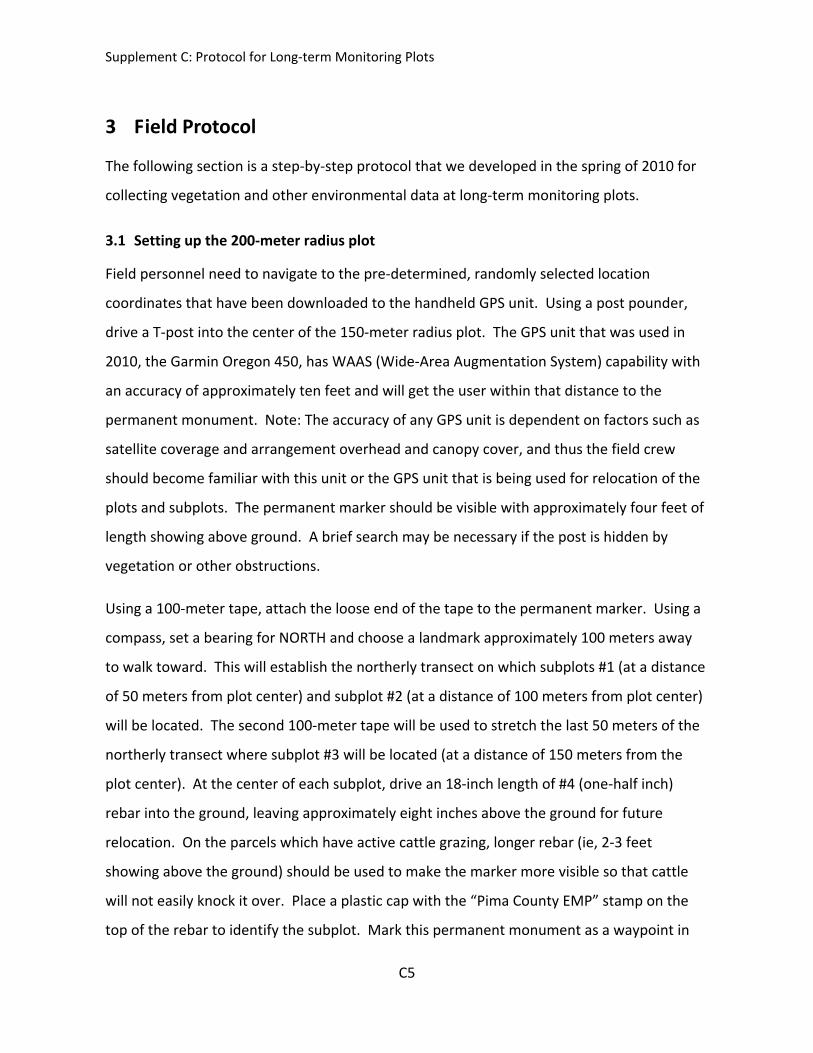
3.1 Setting up the 200‐meter radius plot

Field personnel need to navigate to the pre‐determined, randomly selected location

coordinates that have been downloaded to the handheld GPS unit. Using a post pounder,

drive a T‐post into the center of the 150‐meter radius plot. The GPS unit that was used in

2010, the Garmin Oregon 450, has WAAS (Wide‐Area Augmentation System) capability with

an accuracy of approximately ten feet and will get the user within that distance to the

permanent monument. Note: The accuracy of any GPS unit is dependent on factors such as

satellite coverage and arrangement overhead and canopy cover, and thus the field crew

should become familiar with this unit or the GPS unit that is being used for relocation of the

plots and subplots. The permanent marker should be visible with approximately four feet of

length showing above ground. A brief search may be necessary if the post is hidden by

vegetation or other obstructions.

Using a 100‐meter tape, attach the loose end of the tape to the permanent marker. Using a

compass, set a bearing for NORTH and choose a landmark approximately 100 meters away

to walk toward. This will establish the northerly transect on which subplots #1 (at a distance

of 50 meters from plot center) and subplot #2 (at a distance of 100 meters from plot center)

will be located. The second 100‐meter tape will be used to stretch the last 50 meters of the

northerly transect where subplot #3 will be located (at a distance of 150 meters from the

plot center). At the center of each subplot, drive an 18‐inch length of #4 (one‐half inch)

rebar into the ground, leaving approximately eight inches above the ground for future

relocation. On the parcels which have active cattle grazing, longer rebar (ie, 2‐3 feet

showing above the ground) should be used to make the marker more visible so that cattle

will not easily knock it over. Place a plastic cap with the “Pima County EMP” stamp on the

top of the rebar to identify the subplot. Mark this permanent monument as a waypoint in

C5


the handheld GPS unit using the naming convention “PLOT NAME‐CARDINAL DIRECTION‐

SUBPLOT DISTANCE” (e.g., “BAKERW100M”).

The boundaries of the subplot (i.e., 5 meters in any direction from the subplot center) must

fall at least 10 meters from any road or trail. This eliminates including data for vegetation

and surface features that are directly impacted by human activities. If any subplot at the

50m, 100m or 150m distance from plot center falls too close to a road or trail, move the

location of the subplot center along the transect (either away from or toward the plot

center) until the 10‐meter rule for minimum distance is met.

After completing (1) the establishment of the subplot, (2) field observations and (3) data

collection at the 150‐meter subplot, reel in the tapes and return to the plot center to re‐

orient for the next transect. Replicate the procedures described above to locate the EAST,

SOUTH, and WEST transects following a clockwise pattern (as read on a compass face) and

establish subplots #4‐5‐6 (EAST transect), #7‐8‐9 (SOUTH transect) and #10‐11‐12 (WEST

transect) (see Fig. 1.1).

For plots and subplots that have been previously established and marked with permanent

monuments, navigate to the points using the handheld GPS unit. This eliminates the need to

stretch the 100‐meter tapes and will save time for the field crew, assuming the permanent

rebar monuments have not been destroyed or tampered with. A lightweight, handheld

metal detector could prove useful in the relocation of the subplot centers as the vegetation

will surely change over time and the visible rebar above the ground may be hidden by

vegetation or other environmental features. The rebar should have a brightly colored cap to

make it easier to relocate, but these caps deteriorate over time and it cannot be assumed

they will always be visible. For this reason, the field crew should always have a few

replacement caps on hand to replace worn or destroyed caps while in the field. If the rebar

is missing or cannot be relocated after a search within a 10‐meter radius of the subplot

location coordinate, replace the missing rebar with a temporary marker (if the crew has no

rebar in the field) to be replaced with a permanent monument at a later time. Record this

C6


marker with a waypoint in the handheld GPS unit and save using the naming convention

described above.

3.2 Data Collected at Each Subplot

The following section is a step‐by‐step guide to recording data at each of the 12 subplots per

plot. All data is recorded the program’s datasheet (Fig. 3.1).

3.2.1 Surface Features

The first methods to be employed after the establishment/relocation of the subplot are the

visual estimates of cover for “Surface Features” and “Ground Cover” within the 5‐meter

radius subplot. “Surface Features” shall be estimated for the area within a 2‐meter radius

from the center of the subplot, whereas “Ground Cover” shall be estimated within the entire

5‐meter radial area from subplot center. Cover estimates of surface features are to be

completed as the first monitoring component on the subplot in order to minimize the

disturbance to the soil surface by the field crew. Surface features include six (6) classes of

particle sizes and exposed bedrock that make up the ground surface, including:

(1) FINE 0‐2mm diameter

(2) GRAVEL FINE 2‐16mm diameter (ant to beetle)

(3) GRAVEL COARSE 16‐64mm diameter (beetle to baseball)

(4) COBBLE 64‐256mm (baseball to basketball)

(5) BOULDER >256mm (larger than basketball)

(6) BEDROCK exposed bedrock

C7


Figure 3.1. Datasheet for Long‐term monitoring plots. Plot Name:_______________ State Plane Coordinates: _________________

___________________

Cardinal Direction: N S E W Subplot: 50m 100m 150m Observers: ___________________________________________________ Date:

_________________ GROUND COVER SOIL COVER (5M) %

COVER SURFACE FEATURE (2M) % COVER

BARE FINE 0-2mm PER. GRASS GRAVEL FINE 2-16mm (ant to beetle) ANN. GRASS GRAVEL COARSE 16-64mm (beetle to

baseball)

FORB COBBLE 64-256mm (baseball to basketball) SUBSHRUB BOULDER >256mm (larger than basketball) SHRUB BEDROCK (exposed bedrock) TREE BIO SOIL CRUST (cyanobacterial crust) LITTER WATER (pool or flowing) SNAG MOSS BIO SOIL CRUST

POINT QUARTER NE SE SPECIES DISTANCE RADIUS SPECIES DISTANCE RADIUS PER. GRASS

SUBSHRUB SHRUB TREE SW NW SPECIES DISTANCE RADIUS SPECIES DISTANCE RADIUS PER. GRASS

SUBSHRUB SHRUB TREE COUNTS

SUBSHRUB - 2M 5M SHRUB - 2M 5M TREE 5M SPECIES COUNT SPECIES COUNT SPECIES COUNT

C8


BELT TRANSECT NOTE: DO NOT DOUBLE-COUNT AT SUBPLOT CENTER!

CARDINAL DIRECTION

SPECIES

BASAL

COVERAGE DISTANCE

CARDINAL DIRECTION

SPECIES

BASAL

COVERAGE DISTANCE

ROBEL POLE (CM) START: FINISH: TIME: NORTH EAST SOUTH WEST

C9


BIOLOGICAL SOIL CRUST, or cyanobacteria, is a living, organic component of the “Surface

Features” measurements because the presence (or absence) of these crusts is an indicator of

soil stability and disturbance. These crusts, which vary in color and texture from sandy

brown and flat for young crusts to black and lumpy for older crusts, take many years or

decades to become established yet can be instantly destroyed from minor disturbances. It is

important to note their presence within the subplot early on to avoid trampling while

performing field observations.

WATER, whether flowing or standing, is also included in the “Surface Features” component

of the sampling design as it can be indicative of microsite features (e.g., tinajas, ephemeral

streams) and can help explain localized conditions of the primary 150‐meter radius plot.

“Surface Features” cover estimates are to be made within a 2‐meter radius from the center

of each subplot. Because this measure is an estimate of a single “layer” of cover and does

not account for vertical strata or height classes where cover may overlap (such as the case of

overlapping tree and shrub canopy), the total cover should equal to 100%. In the case of

estimates made for “Ground Cover” wherein canopy cover could overlap, it is possible for

the total estimated coverage to equal to more than 100% because height classes and

overlapping vertical strata are also considered.

When estimating cover for surface features, it can be helpful to begin the estimation with

the feature that appears to be dominant, if indeed there is a dominant feature. For

example, if at least two of the four subplot quadrants are entirely made up of exposed

bedrock, you know that at least 50% of the total 100% coverage will be classified as

“BEDROCK”. This will make it easier to estimate the other particle classes because you can

begin estimating from a smaller area, thereby reducing extent of the area to visualize and

working your way down from most dominant size class to the least dominant size class. Of

course, a dominant size class may not always be present or obvious which can make it more

difficult to visually aggregate particle sizes and then estimate coverage for the individual size

classes for the entire 2‐meter radius area of estimation. Training tools (e.g., Figure 3.2) such

C10


as a small quadrat representing, for example, 10% of the 2‐meter area to be estimated can

be helpful in reducing inter‐observer variability and having a tangible basis to begin the field

work and making visual estimates.

Example of 30% cover for surface

features/ground cover in four

scenarios

Example of 50% coverage for

surface features/ground cover in

four scenarios

Figure 3.2. Examples of percent cover estimates. Figure courtesy of the Southwest Regional

Gap Analysis Project.

C11


Estimating “Ground Cover” generally follows the same procedures as estimating “Surface

Features” as mentioned in the above section. The exception is that it is estimated for the

entire area of the 5m radius subplot (rather than the area of 2m radius for “Surface

Features”. The grand total of percent ground cover may well exceed 100% due to the fact

that overlapping vertical strata (i.e., tree canopy hanging over shrubs or grasses) will be

counted separately, thus the same area of ground may be covered by vegetation in more

than one category and dually counted more than once.

The categories to be estimated for “Ground Cover” are as follows:

• Bare ground – includes exposed ground that has no vegetation growing on it, which

may include soil, gravel, cobbles, boulders and/or bedrock

• Perennial grass

• Annual grass

• Forb – includes annuals that are not grasses but lack the woody base of a shrub

• Subshrub – includes perennial plants with a woody base that are < 0.5M in height

• Shrub – includes perennial plants with a woody base that are >0.5M and <2M in

height

• Tree – includes perennial plants with a woody base that are >2M in height

For Subshrub, Shrub, and Tree, a single plant species may well fall into any of these three

categories because the categories are based on height measurements at the time of the

survey, not the maximum height of that particular species or growth form. For example, the

saguaro cactus, depending on its age and available resources, could fall into any of the three

categories. A juvenile saguaro may fall into the Subshrub or Shrub category depending on its

height, while a mature saguaro will fall into the Tree category because mature saguaro cacti

grow to heights in excess of 2 meters.

Plants that are rooted outside of the subplot but have live canopy which is overhanging into

the subplot should be included in the estimation of ground cover for that growth form

category.

C12


The height of a plant should be measured to the highest point of live vegetation on the

plant. For example, a mesquite tree that has dead material in the canopy may measure over

2m in total height, but if the live growth on the plant measures under 2m and the dead

material in the crown of the canopy puts it over the 2m cut‐off, the tree should be counted

as a Shrub, not a Tree.

• Litter –dead plant material such as grasses, leaves, twigs, bark and cactus carcasses

• Snag –any dead plant that is still rooted in the ground

• Moss –any type of moss that is attached to the ground surface, rocks or other

environmental features

• Biological soil crust –biological crust that is attached to the ground surface or to any

environmental feature

When estimating Ground Cover, as is the case with Surface Features, it can be worthwhile to

identify which category is dominant and begin with that feature working down to the least

dominant feature. In some cases, it may be desirable to start from the least dominant

feature and work your way up to the most dominant feature, depending on the qualities of

the site. With two observers, and especially if it is early in the field season or the observers

have not worked closely together in estimating vegetation cover, it is useful to compare

estimates and discuss the differences between the observations, why they are different and

how to compromise on an agreed‐upon estimate of cover. The goal of long‐term monitoring

is precision. The detection of trends over time is accomplished by systematic, repeatable

observations that are as accurate as possible yet repeatable over time. A highly accurate

survey that is not repeatable has little utility in detecting trend over time.

The overwhelming tendency when estimating cover is to overestimate. Lay persons and

seasoned professionals alike in the field of vegetation surveying and cover estimation tend

to not only overestimate, but also to vary in terms of their cover estimates of vegetation on

the same site. There are training tools available to help with estimating cover, which are not

different than the tools mentioned in the “Surface Features” section. The tools should be

C13


relative to the plot that is being surveyed (ie, the training tool should represent an intuitive

and logical sub‐area of the total plot area, such as 10% or 25%). These tools can be anything

from a square quadrat made of PVC or rope, a hula‐hoop, or cloth cut to a certain size and

shape to meet the training needs of the field crew. We would encourage future field crews

to use these training tools.

3.2.2 Point Quarter

The “Point Quarter” method is used to determine the distance from the center of the

subplot to the nearest: 1) Perennial grass; 2) Subshrub; 3) Shrub; and 4) Tree in each of the

four quadrants of the subplot (ie, NE, NW, SE, SW). The measure of interest is an index to

density. The datasheet should clearly identify the quadrant direction and the observer must

be careful to enter the data in the appropriate field based on the subplot quadrant which is

being observed. Although it is not absolutely necessary to perform the point quarter

method in the same directional sequence each time, doing it in this fashion creates a

methodical, systematic habit for the observer and thus makes him/her less prone to enter

the data in the wrong field (i.e., entering data for the SE quadrant in the fields for the SW

quadrant). The three (3) primary components of data collection for the point‐quarter

method include: 1) Species; 2) Distance (from subplot center); and 3) Radius (from basal

center to median extent of canopy). These fields are clearly labeled on the datasheet (Fig.

3.1). Plants observed should be identified to species‐level if possible and recorded as a six‐

letter code drawn from the first three letters of the plant’s genus followed by the first three

letters of the plant species (i.e., Krameria parviflora = KRAPAR). In the rare instance that two

plant species have the same six‐letter code, create an identifier such as a “1” or “2” after the

six‐letter code that clearly distinguishes the two codes and plant species from each other to

eliminate confusion during data processing.

The “Point Quarter” method measures the distance from the subplot center to the nearest

perennial grass, subshrub, shrub and tree. The thresholds, or cutoffs, for maximum distance

from subplot center to be measured to each type of growth form are:

C14


• Perennial grass 10m

• Subshrub 10m

• Shrub 25m

• Tree 25m

If there is not a representative specimen for the that quadrant, mark “NA” on the datasheet.

As a suggestion, one intuitive method is to begin with the NE quadrant and work through the

observations of each quadrant in clockwise fashion as if looking at the face of a compass,

ultimately ending with observations in the NW quadrant. These measurements can be done

with a tape measure or a laser rangefinder and should be measured to the nearest tenth of

one meter. (Note: Most rangefinders only measure to the nearest meter, with no decimal

places.) These measurements can be used for purposes of analysis including spatial

distribution of species across a site and frequency of individuals relative to plot center;

inferences can be made regarding nutrient availability, water resources and disturbances.

The”Point Quarter” method is typically a method that is quick to perform and one that can

be done with a high degree of accuracy.

The objective of the point quarter method is to accurately measure the distance from the

center of the subplot to the center of the base of the plant being observed, in a straight line.

If measuring with a tape, be sure that the tape is horizontally flat with no kinks, parallel to

the ground, and makes a straight line from the rebar at the center of the subplot to the

center of the base of the plant. The easiest way to do this is to work with another member

of the crew, whereby one member stands with the tape reel or metal pocket tape at the

center of the plot and the second member walks the end of the tape to the center of the

base of the plant to be observed. Holding the tape low to the ground makes it easier to

accurately measure the base of a tree, for example, as opposed to having it a few feet above

the ground and eye‐balling where the tape actually intersects with the center of the base of

the tree.

C15


Of course, certain sites do not allow for this ease of measurement as the vegetation may be

too thick or the nearest plant to be observed is far enough from the subplot center that the

tape cannot hold its form and introduces error into the measurement. In this case,

“shooting” the plant with the rangefinder is the best method to employ as it is time‐efficient,

accurate to the nearest meter and can be used in a variety of landscapes as long as there is a

clear line of sight from the observer to the plant. It is useful to become familiar with the

rangefinder and understand its tolerances for distance. It is also helpful to check the

accuracy of the rangefinder from time to time by laying out a length of tape such as 25M and

having a crew member stand at each end of the tape and shoot the distance to find out if

there is any error coming from the rangefinder when determining straight‐line distances.

Another caveat of the rangefinder, particularly when used to measure the distance to trees

with large or drooping canopies, is that the laser will not penetrate the canopy to the base of

the tree, but will be reflected from the canopy and back to the observer, resulting in an

incorrect measurement. Depending on the confidence of the observer or the needs of the

particular survey or study, a measurement from the base of the tree to the edge of the

canopy may be necessary to compensate for the inaccurate reading, since the center of the

base of the tree is the desired point to be measured to.

The distance thresholds have adopted primarily in the interest of time efficiency in terms of

searching far and wide from the subplot center only to find no plant in that growth form

category to measure. If no individual plant is observed in any quadrant of the subplot, a line

should be drawn in that field to indicate that no individual was found. Do not leave the field

blank because during the data entry and analysis phase it raises a common but avoidable

question – “Did the observer make an observation of “no plant present”, or did they simply

forget to fill in the blank?” In all cases, some entry or notation should be made in every field

on the data sheet to indicate that that component has been completed and that the

observer did not simply forget to “fill in the blank”. If an entry on the data sheet is recorded

in error and needs to be corrected in the field, erase the mark and enter the correct data.

C16


Do not mark through the incorrect notation and note the correct information in the same

field or elsewhere on the data sheet – this introduces confusion during data entry.

3.2.3 Plant Counts

Counting and recording individual plants based on the species and growth form provides

data which can be used to infer species distribution across a plot, estimate the density of

particular species or total vegetation across a plot and offers a picture of the plant diversity

across the site. This method is very straightforward and on most subplot sites should

require less than five minutes to complete. Plants observed should be identified to species‐

level if possible and recorded as a six‐letter code drawn from the first three letters of the

plant’s genus followed by the first three letters of the plant species (i.e., Krameria parviflora

= KRAPAR). In the rare instance that two plant species have the same six‐letter code, create

an identifier, such as a “1” or “2” after the six‐letter code that clearly distinguishes the two

codes and plant species from each other so eliminate confusion during data entry. The

individual plants to be counted fall into three major categories: 1) Subshrub, 2) Shrub, and 3)

Tree. As with other methods performed in this protocol, a plant species may fall into any of

the three categories based on its height. As previously mentioned, the height categories are

as such:

• Subshrub = <0.5m

• Shrub = >0.5m ‐ <2.0m

• Tree = 2.0m or greater

The counts for Subshrub and Shrub are made inside the circular subplot at one of two

distances from center: 2‐meters or 5‐meters. The count for Trees will always be made at

the 5‐meter distance. Accordingly, the rows on the data sheets in the Subshrub and Shrub

categories each have an option to circle “2M” or “5M” depending which distance from

subplot center is being observed for that plot (see “Counts” in Appendix XX). It is crucial to

data processing and analysis that the simple step of circling the distance that is being

C17


counted. Also keep in mind that all twelve subplots in any given plot shall be counted at the

same distance from center. For the 2m subplot counts, any Subshrub, Shrub or Tree should

be identified to species level if possible. The field crew may want to lay out a rope or other

tool to delineate the 2m subplot circle to get an actual visual on the edges and size of the 2m

subplot; with repetition the crew will be able to imagine the borders of the 2m circle and be

able to count all individuals within that area. If an individual plant is in question as to

whether or not it falls within or outside the 2m subplot circle, the crew can lay out tape or

rope to verify. Also, if plants fall on the line of the subplot circle, every other one should be

counted as “in”. For example, if along the 2m subplot circle the crew finds five mesquite

plants that fall into the Shrub category, three (3) of the individuals are to counted as “in” and

two (2) of the individuals should not be counted/included. This pertains only to plants that

are of the same species and fall into the same height category.

These same rules apply to the 5m subplot circle as well, which encompasses the entire area

within the 5m subplot. It may be necessary for a fresh field crew to lay out rope or tape as a

training tool to more easily visualize the area’s borders in order to be confident as to which

plants are “in” and which plants fall “out” of the area and thus are not to be included in the

counts. Again, with repetition the delineation of the 5m subplot area will become easier to

visualize. However, on certain sites such as grasslands with abundant, tall bunchgrasses for

example, it can be difficult even for an experienced crew to visualize the area to include in

the counts and therefore a tool such as rope or tape may be necessary.

The obvious question when performing this component of the protocol is when to use the

2m subplot circle or the 5m subplot circle for counting individual plants. Whichever size is

agreed upon by the field crew and/or project manager, all subplots within the primary plot

are to be observed using the same area. If the crew starts a plot using 2m, the crew should

observe all subplots within that plot at 2m, no exceptions. Observing subplots in the same

plot at different spatial scales does not facilitate data analysis and introduces uncertainty

into the results of analysis. Which spatial scale to use will often be commensurate with the

type of parcel that is being observed, specifically whether it is a rangeland with active cattle

C18


grazing, or not. Normally, the 5m subplot area will be used as it encompasses the entire

subplot and can provide for more diversity and density data since a larger area is being

counted. The 2m subplot circle will be used as the area to count on most (or all) of the

rangeland sites. This is due to the fact that plant species which are browsed by cattle do not

generally reach their growth potential and result in a very high number of small, tightly

spaced individuals that have not had the opportunity to grow to full height. Thus, counting

these individuals in a 2m subplot circle is adequate as that data can be extrapolated to the

area of a 5m subplot very easily with statistical analysis. This is a practical solution in terms

of saving time and energy for the field crew which would be spent tediously counting dozens

or hundreds of tiny individuals.

The final decision of whether to perform the counts using a 2m or 5m subplot circle will

generally follow the type of parcel that is being observed (i.e., active rangeland or not).

However, this is a general rule and if the field crew and/or project manager determines that

the site conditions, data needs, time constraints, or any number of opportunities or

limitations facilitate using one scale or the other, the subplot area may be changed based on

those specific needs. In the scheme of long‐term vegetation monitoring, it is recommended

to perform counts on the same plots in the same fashion so that the data are consistent.

3.2.4 Belt Transect

The belt transect is a method not unlike the “Counts”, which provides data on species

diversity, overall density and basal coverage, the latter being an extremely stable and

reliable indicator to use in long‐term vegetation monitoring. Like the “Counts”, the “Belt

Transect” is to be performed using the same methods but may be performed at different

spatial scales depending on the site characteristics and parcel type (i.e., parcels with active

cattle grazing versus non‐grazed preserves). The decision regarding which scale to

implement will vary ONLY by the plot (NOT by the subplot) and will be decided by the field

crew and/or project manager before the field work begins. This method is simple and

straightforward, but can vary greatly in terms of the time it takes to complete due to the

diversity of sites and the types and density of vegetation. In this method, there are no

C19


height categories for the individual plants to fall into, only the identification and

measurement of individual plants.

The objective of this method is to accurately count the total numbers of plants, identified to

species‐level if possible, and accurately measure the basal coverage of those individuals.

The resulting data will provide information on the diversity, density and coverage of plants

along a 1m linear “belt” for each transect (ie, one‐half meter on each side of the tape).

Plants observed should be identified to species‐level if possible and recorded as a six‐letter

code drawn from the first three letters of the plant’s genus followed by the first three letters

of the plant species (i.e., Krameria parviflora = KRAPAR). In the rare instance that two plant

species have the same six‐letter code, create an identifier, such as a “1” or “2” after the six‐

letter code that clearly distinguishes the two codes and plant species from each other so

minimize confusion during data entry.

The observer should use an implement of 1‐meter length, such as PVC, and walk the transect

(axis) looking for plants within one‐half meter on each side of the tape, using the PVC as a

guide. The decision to include or not include an individual plant is easy – if any part of the

base of the plant falls within the one‐half meter distance from the tape, it is to be included

in the counts and measured entirely. To be clear, the entire width of the plant’s base should

be measured. DO NOT measure only the area of the plant’s base that actually falls within the

one‐half meter; the objective of this method is to measure the change in basal coverage of

the entire plant base in a temporally long‐term monitoring scheme; measuring only part of

the plant’s base would be futile. The measurements are most easily done by aligning the

PVC or other guide in a straight line from the plant’s base to the tape, and recording an

accurate measurement from one side of the plant base to the other, to the nearest

centimeter. It is important to keep in mind that the measuring guide, such as PVC, has its

own width and when measuring the plant base from end‐to‐end using a guide, do not

include the width of the guide in the actual measurement of the plant base. If the

vegetation or other obstacles do not allow for measuring along the tape with the measuring

guide, a physical measurement with another tape may be necessary. Although this scenario

C20


is uncommon, it does occur, and coming away with accurate measurements of basal

coverage (as opposed to eye‐balling or estimating) is one of the objectives of this method.

The first option in terms of spatial scale or arrangement is to perform the belt transect along

the length of each of the four 5m directional axes. One caveat of this method, even for

experienced observers, is the tendency to double‐count at the center of the subplot. With

this in mind, it is important to exclude 1m at the center of the subplot for those two axes

where counting plants would double the counts erroneously. The total area along the tape

to be measured is 18m, which includes five (5) meters along two of the subplot axes, and

four (4) meters along the other two subplot axes.

The alternative option (used primarily on grassland sites with tightly spaced individuals) is to

count the last meter of each tape away from the subplot center. For example, if the tape

reads “50m” at the center of the subplot, the observer will perform the belt transect from

54m to 55m (ie one meter total for each axis, four (4) meters total for the subplot).

Regardless of which option of the two mentioned above is chosen to perform the belt

transect, the data shall be recorded in exactly the same way. The first component is

“Cardinal Direction”, which should be recorded as “N”, “E”, “S”, and “W” depending on the

cardinal direction of the subplot axis being observed. The second component is “Species”

and should be recorded as a six‐letter code following the naming convention mentioned

above. The third and final component is “Basal Coverage Distance” and should be recorded

in centimeters (see Appendix XX).

3.2.5 Robel Pole

The Robel pole is a tool that is 2m in length and graduated with a mark at every 10cm from

the bottom of the pole to the top. The pole can be made of any material; PVC is lightweight,

easy to write on and very packable. This tool is used to estimate vegetation structure and

cover based on the “visual obstruction” method. This method works very well in grassland

systems where coverage is typically continuous from the ground up. However, in uplands

arid systems that do not have continuous grass coverage, using the Robel pole presents

C21


challenges in terms of observations and data analysis. This technique is quick and easy to

estimate on a suitable site, and it can be used to estimate the distribution of biomass on the

subplot site. On the other hand, this technique generally requires two people to efficiently

measure cover (one person to hold the pole, one person to estimate cover). However, in the

case of the circular subplot with rebar at the center of the plot, it is possible to drop the pole

over the rebar and, as long as the bottom of the pole is flush with the ground surface, cover

can be read and estimated by only one person.

Whether one or two persons are measuring cover using the Robel pole technique, the

method remains the same. The pole should stand upright and straight and should be clearly

graduated at every 10cm along the entire 2m length of the pole. It can be helpful to color in

every other 10cm section for easier visibility. The observer should be a distance of 4m from

the pole, which is positioned at the center of the subplot. The observer can use the tapes, or

transects, of the subplot as a guide in order to be certain that he/she is 4m away. The

observer should kneel or bend over so that their eyes are 1m above the ground surface. It is

helpful to actually measure the distance from the ground to the observer’s eyes, especially

with a fresh field crew or at the beginning of the field season, so that they can be confident

in the estimations of cover. One way to do this is for the observer to carry the 1m guide

used for the belt transect as an “eye‐height guide” so that when the observer squats or

bends over, his/her eyes are at the same height as the 1m guide when it is standing upright.

Having the observer’s eyes 1m above the ground is integral to this technique.

From a distance of 4m from the Robel pole and with the observers eyes 1m above the

ground surface, two (2) cover estimations per subplot quadrant are to be measured and

recorded, for a total of eight (8) measurements per subplot. The observer should be looking

toward the Robel pole, which is in place or being held by a crew member, and observing

cover based on the last (highest on the pole) band or mark on the pole that is completely (or

mostly) obscured by vegetation. With practice it is easy to see how the height of the

observer’s eyes above the ground directly affects the measurement, thus it is important to

maintain the 1m height of the observer’s eyes in order to make accurate measurements and

C22


have precision over the long‐term. As with other methods discussed here, it is helpful to

begin and end this technique in the same directional fashion for each subplot as this lends

itself to more consistent and precise data collection.

For example, if the first reading on the Robel pole is made at the 4m mark on the North

transect of the subplot, the observer can make the subsequent observations following a

clockwise pattern (as if looking at a compass face), starting at the North transect and

continuing to the East, South and West transects. One observation should be made along

eash cardinal transect, along with one observation made in the center of each of the four

quadrants. All eight (8) observations should be made from a distance of 4m from the Robel

pole at the center of the subplot.

The shortcoming of the Robel pole technique in some arid systems is that the vegetation is

not continuous from the ground up. For example, a shrub such as desert broom may have a

much narrower basal area than canopy. Thus, if the Robel pole is near the base of the plant,

the bottom of the pole may well be visible and unobstructed by vegetation, but higher up on

the pole the canopy of the plant may obstruct some length of the pole. This is not

continuous coverage along the length of the pole, which the technique is designed to

measure, but coverage that contains gaps along the pole between areas that are obstructed

and areas that are not obstructed. It is difficult to determine how to measure this type of

“discontinuous” coverage as the observation/measurement loses its capacity to depict

structure unless the individual areas of coverage are properly described and measured,

which could introduce much more time spent in the field and in data processing. Simply

aggregating the total amounts of coverage at different spacings along the pole and summing

them into an aggregate measure of coverage would not accurately address the question of

vegetation structure, which is the primary objective of the Robel pole method.

C23

Documents

Leeuw Mining and Exploration