Left Ventricular Electromechanical

Behavior In The Paced Heart

Animal Experiments versus

Finite Element Modeling

Masters thesisJ.P. Hamers

BMTE 08.12

Committee

prof. dr. ir. F.N. v.d. Vossedr. ir. P.H.M. Bovendeerddr. F.W. Prinzendr. ir. H.C. v. Assenir. J.W. Kroon

Eindhoven University of Technology (TU/e)Department of Biomedical EngineeringDivision: Biomechanics and Tissue EngineeringGroup: Cardiovascular Biomechanics

Maastricht, March 2008

AbstractCardiac resynchronization therapy is a procedure that uses a pacemaker to recover the disturbedelectrical impulse conduction of a heart due to, for example left bundle branch block. The degree ofimprovement of cardiac pump function depends on the position of the pacing lead and the timing of thestimulation. To optimize position and timing, mathematical models can be used. Goal of this studywas to test whether the finite element model, developed by Kerckhoffs et al., was capable of simulatingleft ventricular electromechanics for hearts with normal and abnormal impulse conduction. Modelresults were verified using experimental data extracted from magnetic resonance tagging images.Various simple test simulations were performed to test to what extent the procedure for extraction oflocal deformation out of tagging images is accurate. Local deformation was quantified by circumferen-tial, radial and shear strain. Simulation results were compared with analytical solutions. From theseresults it was concluded that the relation between the analytical and estimated strains was non-linearwith increasing deviations for larger strains. A mean difference of −0.008 ± 0.014 in circumferentialstrain was found for an analytical strain of 0.15. Moreover, it turned out that local strain differenceswere dependent on the position within the ventricular wall. Differences were smallest for materialpoints where the displacement vector more or less coincides with the normal vector of the taglinesused for that displacement component. Largest differences were found at locations at angles of multi-ples of 45◦ with respect to the horizontal and vertical taglines.Experimental data showed enlarged moments of onset and peak circumferential shortening and a redis-tribution of total ejection strains for chronically high right ventricular septal paced dogs compared tohearts in sinus rhythm. However, the average ejection strain (SR: -0.121±0.031, PACE: -0.110±0.081),time to onset of shortening (SR: -28.9±16.0, PACE: -39.0±15.7) and time to peak shortening (SR:187.3±69.6, PACE: 153.6±104.1) were not considerably different. On the other hand, the internalstrain fraction was considerably different (SR: 0.0314±0.010, PACE: 0.144±0.046). Because for someregions within the cardiac wall circumferential strains exceed the 0.15, strain estimation errors couldcontribute to larger or smaller differences between the animals and groups. Despite no large differencesin ejection strain and timing, certain patterns are observed. Variation of all parameters increased forincreasing asynchrony.Simulation of pacing results revealed similar patterns. As a consequence of decreased conductionvelocities for the pacing simulation the intra-ventricular delay was increased. This resulted in a redis-tribution of work and ejection strain, thereby reducing cardiac function. Variation in average ejectionstrains (SR: −0.144 ± 0.008, PACE: −0.096 ± 0.093), time to onset of shortening (SR: −24.7 ± 15.5,PACE: −40.9±28.5) and time to peak shortening (SR: 225.2±62.9, PACE: 221.5±104.3) were largerfor increasing asynchrony. Also, there is a substantial difference in internal strain fractions (SR: 0.035,PACE: 0.151).Comparing simulation and experimental results required a time and amplitude normalization withrespect to the ejection phase. Choice of begin and end-ejection appeared to be critical in order todecide whether the mathematical model was able to describe experimental cardiac mechanics accu-rately. Local deformation patterns were not reproduced completely, but, despite a relatively simplemodel, phenomena such as distributions of timing and total ejection strain were in accordance withexperimental data extracted from MRT images. Improvement of the model and analysis is achievedby a better definition of the ejection phase, addition of a right ventricle with the accompanying pul-monary circulation and more insight in the electrophysiology of the heart. This might lead to a betterapproach of experimental results. Overall, the used finite element model is suitable to simulate leftventricular mechanics for normal and abnormal electrical impulse conduction.

ii

SamenvattingCardiale resynchronisatie therapie is een procedure die met behulp van een pacemaker de verstoordeimpulsgeleiding van harten met bijvoorbeeld een linkerbundeltakblok probeert te herstellen. De matevan verbetering van de hartfunctie is afhankelijk van de plaats van de pacedraad en de timing vanimpuls initiatie. Mathematische modellen zijn uitermate geschikt om de optimale plaats en timingte bepalen. Het doel van deze studie was te testen of het eindige elementen model, ontworpen doorKerckhoffs et al.1, in staat was om de elektromechanica van het linker ventrikel zowel met normaleals abnormale impulsgeleiding te beschrijven. Model resultaten werden vergeleken met experimenteledata die verkregen waren met behulp van MR tagging.Om de procedure te testen die uit de tagging beelden lokale deformatie kan bepalen zijn er een aan-tal eenvoudige simulaties uitgevoerd en vergeleken met analytische oplossingen. Hieruit kon wordengeconcludeerd dat de relatie van het verschil tussen de opgelegde en geschatte circumferentiele rekkenniet-linear was. Bij een circumferentiele rek van 0.15 bedroeg het gemiddelde verschil −0.008± 0.014.Bovendien bleek de mate van afwijking plaats afhankelijk te zijn. De kleinste afwijkingen werdengevonden op posities waarvan de verplaatsingsvector min of meer overeen kwam met de normaalvectorvan de taglijn die gebruikt werd om die specifieke verplaatsingscomponent te bepalen. De grootsteafwijkingen werden echter gevonden op posities onder een hoek van veelvouden van 45◦ ten opzichtevan de horizontale en verticale taglijnen.Uit de experimentele data is gebleken dat chronisch pacen van het linker ventrikel hoog in hetrechter ventriculair septum heeft geleid tot een latere begin en piek circumferentiele verkorting eneen herverdeling van de totale ejectierek. Echter, de gemiddelde rek tijdens ejectie (SR: -0.121±0.031,PACE: -0.110±0.081), tijd tot begin verkorting (SR: -28.9±16.0, PACE: -39.0±15.7) en tijd tot piekverkorting (SR: 187.3±69.9, PACE: 153.6±104.1) waren niet verschillend. Daarentegen is de internerek fractie voor beide groepen wel aanzienlijk verschillend (SR: 0.0314±0.010, PACE: 0.144±0.046).Afwijkingen in rekberekeningen kunnen ook bijdragen aan de verschillen tussen beide groepen. Maarer zijn wel patronen zichtbaar, namelijk dat de varianties voor deze parameters groter zijn naarmatede asynchrony toeneemt.De pace simulaties resulteerden in vergelijkbare patronen. Door de geleidingssnelheden te verlagenvoor de pace simulatie konden grotere intra-ventriculaire vertragingen gecreeerd worden en leidde toteen herverdeling van de arbeid en ejectie rek met als gevolg een verslechterde pompfunctie. Variantiesin ejectie rek (SR: −0.144±0.008, PACE: −0.096±0.093), tijd tot begin verkorting (SR: −24.7±15.5,PACE: −40.9 ± 28.5) en tijd tot piek verkorting (SR: 225.2 ± 62.9, PACE: 221.5 ± 104.3) zijn grotervoor toenemende asynchrony. De interne rek fractie is ook voor de simulaties verschillend (SR: 0.035,PACE: 0.151).Om de resultaten tussen de experimenten en simulaties te vergelijken werden de circumferentiele rekkengenormaliseerd met betrekking tot de ejectie fase. Het bleek dat de keuze van begin en eind ejectiebepalend was om te besluiten of het model in staat was om de mechanica van de experimenten tebeschrijven. Lokale deformatie patronen waren niet exact gereproduceerd, maar ondanks een relatiefsimpel model waren de distributies van de tijd tot begin en piek verkorting en de totale ejecierek inovereenstemming met de resultaten van de experimenten die met behulp van MRT verkregen zijn.Het verbeteren van de ejectie fase definitie, het toevoegen van het rechter ventrikel met bijbehorendelongcirculatie en meer inzicht in de electrofysiologie van het hart zou kunnen leiden tot een betere be-nadering van de experimentele resultaten. Over het algemeen is het gebruikte eindige elementen modelin staat om de mechanica van het linker ventrikel voor zowel normale als abnormale impulsgeleidingte simuleren.

iv

Contents

Abstract i

Samenvatting ii

1 General Introduction 1

1.1 Background . . . . . . . . . . . . . . . . . . . . . . . . . . . . . . . . . . . . . . . . . . 1

1.2 Thesis aim and outline . . . . . . . . . . . . . . . . . . . . . . . . . . . . . . . . . . . . 2

2 Magnetic Resonance Tagging 3

2.1 Introduction . . . . . . . . . . . . . . . . . . . . . . . . . . . . . . . . . . . . . . . . . . 3

2.2 Myocardial tagging . . . . . . . . . . . . . . . . . . . . . . . . . . . . . . . . . . . . . . 3

2.3 Determination of two dimensional displacements . . . . . . . . . . . . . . . . . . . . . 5

2.3.1 Method principles . . . . . . . . . . . . . . . . . . . . . . . . . . . . . . . . . . 5

2.3.2 HARP . . . . . . . . . . . . . . . . . . . . . . . . . . . . . . . . . . . . . . . . . 5

2.3.3 SinMod . . . . . . . . . . . . . . . . . . . . . . . . . . . . . . . . . . . . . . . . 7

2.4 Analysis of the tag images . . . . . . . . . . . . . . . . . . . . . . . . . . . . . . . . . . 8

2.5 Test simulations . . . . . . . . . . . . . . . . . . . . . . . . . . . . . . . . . . . . . . . 10

2.5.1 Methods . . . . . . . . . . . . . . . . . . . . . . . . . . . . . . . . . . . . . . . . 10

2.5.2 Results . . . . . . . . . . . . . . . . . . . . . . . . . . . . . . . . . . . . . . . . 13

2.6 Discussion . . . . . . . . . . . . . . . . . . . . . . . . . . . . . . . . . . . . . . . . . . . 17

2.6.1 Magnetic resonance tagging . . . . . . . . . . . . . . . . . . . . . . . . . . . . . 17

2.6.2 Displacement estimations method . . . . . . . . . . . . . . . . . . . . . . . . . 18

2.6.3 Strain calculations . . . . . . . . . . . . . . . . . . . . . . . . . . . . . . . . . . 18

2.6.4 Conclusion . . . . . . . . . . . . . . . . . . . . . . . . . . . . . . . . . . . . . . 19

3 Strain In Healthy And Paced Canine Left Ventricles 21

3.1 Introduction . . . . . . . . . . . . . . . . . . . . . . . . . . . . . . . . . . . . . . . . . . 21

3.2 Materials and methods . . . . . . . . . . . . . . . . . . . . . . . . . . . . . . . . . . . . 21

3.2.1 Experimental protocol . . . . . . . . . . . . . . . . . . . . . . . . . . . . . . . . 21

3.2.2 Magnetic resonance imaging . . . . . . . . . . . . . . . . . . . . . . . . . . . . . 22

3.2.3 Data analysis . . . . . . . . . . . . . . . . . . . . . . . . . . . . . . . . . . . . . 22

3.2.4 Data representation . . . . . . . . . . . . . . . . . . . . . . . . . . . . . . . . . 24

3.3 Results . . . . . . . . . . . . . . . . . . . . . . . . . . . . . . . . . . . . . . . . . . . . . 25

3.4 Discussion . . . . . . . . . . . . . . . . . . . . . . . . . . . . . . . . . . . . . . . . . . . 29

3.4.1 Accuracy of circumferential strains . . . . . . . . . . . . . . . . . . . . . . . . . 29

3.4.2 Timing . . . . . . . . . . . . . . . . . . . . . . . . . . . . . . . . . . . . . . . . 29

3.4.3 Amplitude and time normalization . . . . . . . . . . . . . . . . . . . . . . . . . 30

3.4.4 Conclusion . . . . . . . . . . . . . . . . . . . . . . . . . . . . . . . . . . . . . . 30

v

4 Simulations Of Left Ventricular Electromechanics 31

4.1 Introduction . . . . . . . . . . . . . . . . . . . . . . . . . . . . . . . . . . . . . . . . . . 314.2 Materials and methods . . . . . . . . . . . . . . . . . . . . . . . . . . . . . . . . . . . . 31

4.2.1 Geometry and structure of the left ventricle . . . . . . . . . . . . . . . . . . . . 314.2.2 Electrical activation . . . . . . . . . . . . . . . . . . . . . . . . . . . . . . . . . 324.2.3 Left ventricular mechanics . . . . . . . . . . . . . . . . . . . . . . . . . . . . . . 334.2.4 Hemodynamic coupling . . . . . . . . . . . . . . . . . . . . . . . . . . . . . . . 344.2.5 Numerical implementation . . . . . . . . . . . . . . . . . . . . . . . . . . . . . . 354.2.6 Simulations . . . . . . . . . . . . . . . . . . . . . . . . . . . . . . . . . . . . . . 364.2.7 Data analysis . . . . . . . . . . . . . . . . . . . . . . . . . . . . . . . . . . . . . 37

4.3 Results . . . . . . . . . . . . . . . . . . . . . . . . . . . . . . . . . . . . . . . . . . . . . 384.3.1 Electrical activation . . . . . . . . . . . . . . . . . . . . . . . . . . . . . . . . . 384.3.2 Mechanics and hemodynamics . . . . . . . . . . . . . . . . . . . . . . . . . . . 38

4.4 Discussion . . . . . . . . . . . . . . . . . . . . . . . . . . . . . . . . . . . . . . . . . . . 444.4.1 Electrical activation . . . . . . . . . . . . . . . . . . . . . . . . . . . . . . . . . 444.4.2 Simulation mechanics and hemodynamics . . . . . . . . . . . . . . . . . . . . . 454.4.3 Experimental vs simulation results . . . . . . . . . . . . . . . . . . . . . . . . . 474.4.4 Conclusion . . . . . . . . . . . . . . . . . . . . . . . . . . . . . . . . . . . . . . 53

5 General Discussion 55

5.1 Active stress - sarcomere length relation . . . . . . . . . . . . . . . . . . . . . . . . . . 555.2 Interventricular septal motion . . . . . . . . . . . . . . . . . . . . . . . . . . . . . . . . 555.3 Acute vs chronic pacing . . . . . . . . . . . . . . . . . . . . . . . . . . . . . . . . . . . 565.4 LBBB vs high RV septal pacing . . . . . . . . . . . . . . . . . . . . . . . . . . . . . . . 575.5 RV apex pacing vs high RV septal pacing . . . . . . . . . . . . . . . . . . . . . . . . . 585.6 Conclusion . . . . . . . . . . . . . . . . . . . . . . . . . . . . . . . . . . . . . . . . . . 59

Appendices 60

A Magnetic Resonance Tagging . . . . . . . . . . . . . . . . . . . . . . . . . . . . . . . . 61A.1 Nuclear Magnetic Resonance . . . . . . . . . . . . . . . . . . . . . . . . . . . . 61A.2 Construction of MR images . . . . . . . . . . . . . . . . . . . . . . . . . . . . . 62A.3 Spatial modulation of longitudinal magnetization . . . . . . . . . . . . . . . . . 63

B Green-Lagrange strains for the test simulation . . . . . . . . . . . . . . . . . . . . . . . 65C Data analysis . . . . . . . . . . . . . . . . . . . . . . . . . . . . . . . . . . . . . . . . . 66

C.1 Singular value decomposition . . . . . . . . . . . . . . . . . . . . . . . . . . . . 66C.2 Estimation of timing parameters . . . . . . . . . . . . . . . . . . . . . . . . . . 67

Bibliography 69

Erratum 72

vi

Chapter 1

General Introduction

1.1 Background

The heart is a biological pump providing blood flow through the circulatory system. The right andleft ventricle (RV and LV) of the heart supply the force that propels the blood through either thepulmonary or the aortic artery. In order to develop the necessary force, ventricular muscle is a highlyorganized continuum of muscle fibers. Each fiber contains myocytes embedded in an extracellularconnective tissue matrix, that can develop force and shorten in response to an electrical impulse2–4.

In a healthy heart, around seventy times a minute an action potential is initiated at the sinoatrialnode, or SA-node, from where it is conducted to the ventricular muscle through the His bundle and leftand right bundle branches to the fast conducting Purkinje fibers. Once the impulse reaches the ends ofthese fibers it is transmitted slowly by the ventricular muscle fibers from endocardium to epicardium.2

Endocardial activation is earlier compared to epicardial activation, resulting in a transmural activa-tion difference of approximately 40 ms.1,5,6 Despite the gradient in electrical activation, contractionis relatively synchronous. This suggests that myocardial tissue is able to synchronize contraction, butit is not known yet what mechanism controls this behavior.

However, for hearts with abnormal ventricular impulse conduction, such as with left bundle branchblock (LBBB), the electrical asynchrony is increased, leading to asynchronous mechanical behavior.In these cases local contraction not only differs in onset of contraction, but also contraction patternsare different.7,8 Consequences of local abnormalities in contraction patterns are adverse hemodynamiceffects and abnormal distributions of myocardial work and blood flow8–11. With a lower cardiacoutput (CO), ejection fraction (EF) and maximal left ventricular pressure rise (LV (dp/dt)max), butsimilar global oxygen consumption as a healthy LV12, it can be concluded that myocardial efficiencyis decreased. Moreover, animal studies revealed structural changes on a long term, like ventriculardilatation and asymmetric hypertrophy9,13. Asynchrony becomes even more pronounced due to thisremodeling process because of the increased pathway length and wall mass.

As asynchronous activation results in ventricular dysfunction, resynchronization of the electrical im-pulse can improve cardiac performance and can lead to inverse remodeling14. Resynchronization canbe achieved either by single site or biventricular pacing. In both cases timing of activation and lead po-sitions are of great importance for the amount of intraventricular delay and therefore cardiac function.An issue to be solved is finding the optimal combination of timing and lead position. Conventionallocations for single site pacing are either the right endocardial apex or the postero-lateral left ventricu-lar epicardial wall. For biventricular pacing a combination of both sites is predominantly used. Manyacute and chronic pacing studies have shown improvements in the parameters of cardiac function for

Chapter 1. General Introduction 1.2. Thesis aim and outline

both settings in LBBB hearts.15–18 However, chronic effects of alternate pacing sites on the RV orLV are not structurally investigated yet. It might well be that there are other pacing sites that willincrease cardiac function even more or give rise to a larger percentage of responders to this treatment.Therefore, in Maastricht a comprehensive animal study has been set up in order to relate chronicconventional and alternate site pacing to structural, functional and cellular changes within heart wall.The results of the study may have a direct impact on the strategy to follow with regards to the site ofventricular pacing.

A useful method to examine influences of alternate lead positions on cardiac performance is by mathe-matical finite element modeling (FEM). These models can not only reveal valuable information aboutthe global function of the heart, but more importantly lead to a better understanding of the con-tribution of local deformation on left ventricular hemodynamics. Furthermore, they can be used foroptimization of timing and lead positions. Kerckhoffs et al.1 have developed a FE model of a humanLV that was able to simulate electromechanics of healthy LV’s and LV’s that were paced at the leftventricular free wall and right ventricular apex. However, alternate pacing sites such as high RV septal,transseptal or the left ventricular apex were not examined.

1.2 Thesis aim and outline

The overall aim of this study was to investigate if the mathematical FE model developed by Kerckhoffsis able to simulate left ventricular deformation of normal hearts and hearts with abnormal electricalactivation patterns, induced by an artificial pacemaker. To this end, cardiac deformation, as computedwith the model for various pacing sites, was compared to deformation measured in animal experimentswith magnetic resonance tagging (MRT).

Chapter 2 discusses the relevant techniques for motion measurement and the subsequent straincomputations. Besides, several simple tests were performed for verification of the applied method.Subsequently, chapter 3 contains a quantitative analysis of experimental results of hearts with nor-mal sinus rhythm (SR) and during ventricular pacing. Results of left ventricular simulations in aphysiological and paced setting are discussed in chapter 4. Finally, chapter 5 contains a general dis-cussion to what extent the FE model is able to describe local left ventricular mechanics. Furthermore,recommendations for future research are mentioned briefly in this chapter.

2

Chapter 2

Magnetic Resonance Tagging

2.1 Introduction

MRT is a tool that is capable of visualization of ventricular motion during the cardiac cycle. Al-gorithms are able to extract parameters like circumferential strain, timing and the internal strainfraction (ISF)19 from tagging data. These parameters are used to characterize ventricular condition.This chapter will illustrate and discuss the tools available for analysis of left ventricular function anduses a set of test simulations for verification of the applied method. In appendix A the principles ofmagnetic resonance imaging (MRI) are discussed.

2.2 Myocardial tagging

Zerhouni et al. (1988) demonstrated that tissue tagging is a reliable method for motion measurementof the heart. Specified regions within the myocardium can be labeled to serve as markers duringcontraction. MRT is based on applying local changes in longitudinal magnetization at end-diastole.20

The modulated longitudinal magnetization results in a corresponding intensity modulation in the fi-nal image, appearing as light and dark bands or tags (figure 2.1). Because magnetization is a tissueproperty these tag lines move along with the tissue during deformation. The deformed tag patternreflects the underlying motion of the heart wall.14

Figure 2.1: MRT im-ages of a short-axisview of a dog heartwith taglines in x andin y direction at a cer-tain time during thecardiac cycle.

Chapter 2. Magnetic Resonance Tagging 2.2. Myocardial tagging

Because the heart is beating, it is obvious that a single static magnetic resonance (MR) image provideslimited information of cardiac motion. A series of images, made at regular intervals during the car-diac cycle, gives additional information. Providing good contrast between the tagged and non-taggedmyocardium and sufficiently high temporal and spatial resolution is essential to track the saturationpatterns. MRT is therefore a time consuming procedure and it is impossible to acquire the datawithin one heartbeat. Because it is assumed that there will be no significant difference in position andmechanical behavior of the heart for each beat, the acquisition of one frame of the cine is distributedover several cardiac cycles (segmented k-space21–23). However, the subject’s breathing motion causesmotion of the heart relative to the MR scanner, resulting in unwanted blurring. To avoid breathingmotion during acquisition the heart is imaged within a single breath hold.

Relaxation of the longitudinal magnetization reduces the amplitude of the modulation. At the end ofthe cardiac cycle the signal-to-noise-ratio (SNR) is therefore decreased, leading to increased artifactsin motion computations. This tag fading is dependent on the time constant T1, which is in turndependent on the magnetic field strength.

Cardiac motion from the base towards the apex of the heart during the ejection phase causes throughplane motion. Through plane motion is defined as motion of material points in the direction perpen-dicular to the fixed image plane. Therefore, tag lines can either disappear or reappear, depending onthe reference situation (figure 2.2).At end-diastole the magnetization of blood inside the cavity is also spatially modulated, hence ven-tricular wall and cavity can not be distinguished. Because magnetization is a material property taglines will disappear when blood moves outside the image plane. The same holds for material pointswithin the wall near the base where through plane motion is maximal.

tag planes

material point referenceapparent material point

image planematerial point referenceapparent material point

tag planes

image plane

Figure 2.2: The black spot corresponds to a material point in the reference state (end-diastole) where the taglines are applied. The white spot corresponds to the same material point but at a certain time during the cardiaccycle. Due to motion of the base towards the apex, material points will displace. Because the image plane is fixed,a material point can either move into the image plane or move out of the plane.

Tracking cardiac motion requires multiple short-axis slices throughout the heart. Scanning time isproportional to the product of the repetition time (TR) and the number of phase encoding steps (seeappendix A). TR is the amount of time between two successive pulse sequences applied to the sameslice. In between the pulse sequences there is a lot of unused time. Reducing scanning time is possibleusing one spatial gradient slice selection pulse but applying different radio frequency (RF) pulses inbetween two pulse sequences. This makes it possible to collect motion data for several slices withinone sequence.

Investigation of the entire contraction phase requires triggering of the tagging pulses on the rightmoment. Most common is to electrographically trigger shortly after the R-wave of the QRS complex.Therefore, the first frame of the cine is acquired at end-diastole. Worth to notice is that there is atime difference between image tagging and the actual data acquisition. About 20 ms after triggering

4

2.3. Determination of two dimensional displacements Chapter 2. Magnetic Resonance Tagging

the tag lines are applied and in turn 15 ms later the data acquisition is started. This results in a 35ms delay and so loss of information about early cardiac motion.

2.3 Determination of two dimensional displacements

2.3.1 Method principles

Tag data contains information about displacements of a certain point in the direction perpendicular tothe tag line.24 Displacements in x and y direction can be extracted using different sets of tag images.Orientation of the tag lines is dependent on the direction of the gradient pulse.

In the past years, important progress has been made in the field of displacement computations. Pub-lished methods include active contour models25, optical flow26,27 and harmonic phase (HARP)28. Dueto its automatic nature, HARP tracking is a powerful tool for motion extraction. The basic idea ofthis method is to regard the tag pattern of spatial modulation (SPAMM) images as a spatially peri-odic signal that is frequency modulated during cardiac deformation. Therefore HARP focuses on thespatial phase and frequency of the tag signal.28–30 Tag line displacement is assessed by tracking itsphase angle over the cardiac cycle, normally starting at a reference frame with undeformed tag pattern(Lagrangian approach). Deformation induces phase shifts and those shifts are related to motion.

Suppose a one dimensional signal represents the spatial image intensity (I1(x)) of a piece of tissue attwo different times in case of simple displacement and compression of tissue (figure 2.3). The solidline represents the image intensity at the reference configuration and the dashed line indicates I1(x)after deformation. At each pixel, displacement (ux) is calculated according to equation 2.1.

ux =φref − φdef

fdef[mm] (2.1)

with φdef the local phase in the deformed configuration, φref the local phase in the reference configu-ration and fdef the local spatial frequency, in linepairs per mm, in the deformed configuration. Onelinepaire represents a total phase change of 2π. Simple displacement of 1

8 mm in positive x-directionas in the left panel of figure 2.3 induces phase shifts while the frequency remains constant. At pointA a phase shift of 1

2π and a frequency of 4π/mm resulted in the applied displacement. Suppose thetissue is compressed, thereby increasing the frequency of the tag pattern (right panel of figure 2.3). Inthis case the phase difference at point A is π − 3

2π = − 12π and with a frequency of 6π/mm, ux = − 1

12mm.

2.3.2 HARP

With line tagging the image is amplitude modulated in one direction with a certain sinusoidal tagmodulation function. Depending on the orientation of the tag lines this modulation function is eithera function of x (vertical lines) or a function of y (horizontal lines). Suppose a one dimensionalhomogeneous piece of tissue with initial constant magnitude I0 throughout the image is modulatedwith a sinusoidal function m(x):

m(x) = c1 + c2 cos(φ) = c1 + c2 cos(ω1x + φ0) (2.2)

where c1 and c2 are constants, ω1 is the spatial frequency of the tag lines and φ0 determines the phaseat x = 0. Multiplication of the original image with m(x) results in the tagged image:

I1(x) = I0 [c1 + c2 cos(ω1x + φ0)] (2.3)

5

Chapter 2. Magnetic Resonance Tagging 2.3. Determination of two dimensional displacements

0 0.2 0.4 0.6 0.8 1

−1

−0.5

0

0.5

1

x [mm]

0 0.2 0.4 0.6 0.8 1

−1

−0.5

0

0.5

1

I 1 [−]

ux

A’

A

A’

Au

x

Figure 2.3: Left: The relation between position and image intensity (I1(x)) in the reference configuration isdisplayed as a solid line. Simple displacement of 1

8mm result in the dashed line. φA = π, φA′ = 1

2π and the

frequency in the deformed state is 4π/mm resulting in the applied ux. Right: Again, the solid line illustrates imageintensity at the reference state while the striped line after compression of the 1D tissue. φA = π, φA′ = 3

2π and

the frequency is 6π/mm resulting in a displacement of − 1

12mm.

with I0 the image intensity of the non-tagged tissue.

Since HARP focuses on the local spatial phase, complex notation of equations is more convenient forphase determination. Equation 2.3 gets the following appearance:

I1(x) = I0

[

c1 +1

2c2

(

eiφ0eiω1x + e−iφ0e−iω1x)

]

(2.4)

The fundamental principle of HARP is using the Hilbert transformation for extraction of the positivefrequency. Hilbert transformations exist of Fourier transformation, isolation of one of the two complexterms in the real signal followed by inverse Fourier transformation. Extraction of only one componentof the signal enables splitting the signal in a frequency and a phase. Equation 2.5 defines the Fouriertransform of the tagged image.

K1(ω) =∫

∞

−∞I1(x)e−iωxdx

= I0

∫

∞

−∞

[

c1 + 12c2

(

eiφ0eiω1x + e−iφ0e−iω1x)]

e−iωxdx

= πI0

[

c1δ(ω) + c2eiφ0δ(ω − ω1) + c2e

iφ0δ(ω + ω1)]

(2.5)

It is clear that the tagged image is composed of an offset with frequency ω = 0 and two frequencies ω1

and -ω1. Next step of the Hilbert transformation is bandpass filtering resulting in deletion of the offsetand negative frequency. Two different filters are used; a low and a high bandpass filter each centeredaround the initial frequency of the tag pattern (ω1) with a relative bandwidth of 1.0. Frequencydistributions of the reference image and deformed image are normalized by ω1 in order to computethe relative local frequency.

P1(ω) = K1(ω)B(ω)

= πc2

I0eiφ0δ(ω − ω1)

(2.6)

6

2.3. Determination of two dimensional displacements Chapter 2. Magnetic Resonance Tagging

B(ω) indicates the low or high frequency bandpassfilter. Inverse Fourier transformation of P1(ω)yields:

p1(x) = 12π

∫

∞

−∞P1(ω)eiωdω

= I0

2c2eiφ0eiω1x

= I0

2c2[cos (ω1x + φ0) + i sin (ω1x + φ0)]

= I0

2c2eiω1x+iφ0

(2.7)

The resulting signal is a complex signal with a real part equal to the original signal with any offsetremoved and an imaginary part equal to the original signal shifted 90o in phase.

The standard HARP procedure will continue with calculation of the phase angle, θ1(x) = ω1x + φ0.The tangent of the quotient of the imaginary and real parts equals the angle:

tan θ1(x) =Im (p1(x))

Re (p1(x))=

sin (ω1x + φ0)

cos (ω1x + φ0)(2.8)

The angle, wrapped into the range (−π, π], can be computed from the inverse tangent in equation2.8 by taking into account the sign of the numerator and denominator. This quantity is referred asthe wrapped angle ϕwr

1 (x). It is straightforward to unwrap the sampled signal of ϕwr1 (x) by removing

phase-jumps larger than 180◦ to obtain the true phase. The unwrapped angle ϕ1(x) then equals θ1(x)except for some unknown multiple of 2π phase-offset.

The spatial derivative of the phase angle represents the local instantaneous frequency, k1(x):

k1(x) =d

dxϕ1(x) (2.9)

The instantaneous frequency is directly related to the local deformation of the imaged tissue. Beforedeformation k1(x) is independent of x and equals the tag frequency ω1. For the one-dimensional pieceof tissue the stretch of an infinitely short line segment aligned with the x-axis, with length dl0 beforedeformation and length dl after deformation is given by:

λ(x) =dl

dl0=

k1(x)

k2(x)=

ω1

k2(x)(2.10)

Instantaneous frequency k2(x) after deformation is computed the same way as the frequency beforedeformation.

2.3.3 SinMod

Recently, Arts has introduced an improved HARP method (SinMod) for motion measurements andfirst relates phase differences to displacements whereafter strain calculations can be performed. Thismethod is based upon cross correlations between the reference image and the image of which displace-ments need to be calculated. Suppose after the same filtering procedure the reference and deformedimage after a certain time t are described by equation 2.11.

Iref,lf =√

ω1

ωA1e

iφ1 Iref,hf =√

ωω1

A1eiφ1

Idef,lf =√

ω1

ωA2e

iφ2 Idef,hf =√

ωω1

A2eiφ2

(2.11)

7

Chapter 2. Magnetic Resonance Tagging 2.4. Analysis of the tag images

with ω the local signal frequency, A1 and A2 the local positive real amplitudes of the filtered imagesand φ1 = i (ωx + φ0) and φ2 = i (ω (x + ux) + φ0) the phases of the images. Subscripts lf and hfindicate low and high frequencies, respectively.

The following cross correlation products were determined, where complex conjugation is indicated bya bar symbol on top.

Plf = Iref,lf Iref,lf + Idef,lf Idef,lf = ω1

ω

(

A21 + A2

2

)

Phf = Iref,hf Iref,hf + Idef,hf Idef,hf = ωω1

(

A21 + A2

2

)

Pcc = Iref,lf Idef,lf + Iref,hf Idef,hf =(

ω1

ω+ ω

ω1

)

A1A2eiωux

(2.12)

Plf and Phf are real, representing total power in the band, biassed to low and high frequencies, respec-tively. Pcc represents complex cross correlation, while summing the low and high frequency distribu-tions. Because cross correlation requires that both signals have a good SNR it is important that on alocal level enough information is available for displacement estimations, i.e. signal amplitudes A1 andA2 should be larger than the noise amplitude. For a high quality fit these amplitudes should be aboutequal and the contribution of noise should be little. If, on a local level, the amplitude of one or bothof the images is to low, based on a threshold, information from the surroundings is used to obtain anestimation of the phase angle (equation 2.13). This correction is useful if amplitude and phase aredistributed in an inhomogeneos manner.

T =2|Pcc|

Plf + Phf=

2A1A2

A21 + A2

2

(2.13)

From equation 2.14 frequency ω and displacement ux in a direction perpendicular to the tag lines canbe solved.

u =arg (Pcc)

√

Plf

ω1

√

Phf

= ux

ω

ω1

√

ω1

ω√

ωω1

= ux

ω

ω1

ω1

ω= ux (2.14)

A map of displacements in x-direction is obtained by application of equation 2.14 for every pixelwithin the image. Center frequency ω1 is the same for all pixels and is calculated by dividing 2π bythe intertag distance. However, the local frequency ω may differ from this center frequency althoughdeviation should not exceed the width of the bandfilter. Displacements in two dimensions are foundby subsequent application of this method for a wave perpendicular to the first one.

2.4 Analysis of the tag images

In this section the analysis of the images produced by MRT will be described. Definition of the regionof interest (ROI), reference point calculation and eventually displacement calculations are importantfor strain estimations. Information about displacement calculations can be found in section 2.3.

Region of interest

The first steps are drawing the ROI and the right ventricular junction points (RVJP’s) for each slice incine images of the heart (figure 2.4). The RVJP’s are located near the anterior and posterior regionsand are used for septum definition. Two polygons are drawn by the user, specifying the boundaries of

8

2.4. Analysis of the tag images Chapter 2. Magnetic Resonance Tagging

the left ventricular wall, i.e. the endocardial and epicardial border. Papillary muscles and or blood areexcluded from the ROI because this will influence the displacement calculation. To avoid this problemcontours are drawn with a margin about 10% around the ventricular wall (figure 2.4).If no cine image sequence is available for every slice the best tagged image sequence should be used .In that case the first frame of the image cannot be used because at this time the tag lines are appliedand no distinction can be made between the left ventricular wall and the cavity.

Figure 2.4: Left: An example of adrawn ROI with the two black linesindicating the endocardial and epi-cardial border, respectively. Thetwo black spots indicate the poste-rior (P) and anterior (A) RVJP’s.Right: The solid lines indicate theendo- and epicardial border whilethe dashed lines indicate the ROIwith a margin of 10% on both sidesof the ventricular wall.

papillarymuscles

Reference image

Strains are computed with respect to a reference configuration and in this case the first frame ischosen to be the reference. Because the ROI is drawn at a later time, the subsequent step is movingthe ROI’s of all the slices with calculated motion to the reference frame. Motion is calculated accordingto equation 2.14.

Strain computations

Deformation of the heart wall can be quantified by circumferential, radial and shear strain. Straincomputations require displacement information between the deformed and undeformed state and canbe calculated according to equation 2.15.

E =1

2

(

FT · F − I

)

(2.15)

with E the Green-Lagrange strain tensor. Deformation tensor F describes the change in position ofmaterial points due to deformation and rotation and equals:

F =(

~∇0~x)T

= I +(

~∇0~u)T

(2.16)

Combining both equations results in a relation between the displacements and the Green-Lagrangestrain.

E =1

2

(

(

~∇0~u)

+(

~∇0~u)T

+(

~∇0~u)

·(

~∇0~u)T)

(2.17)

In order to obtain gradients in displacements in x as well as in y direction, convolution is used insteadof discrete differences due to sensitivity to noise. Smoothing with a hanning window will reduce thenoise within the resulting cartesian strain maps.

9

Chapter 2. Magnetic Resonance Tagging 2.5. Test simulations

Since MRT yields displacements ux and uy with respect to a Cartesian coordinate system {~ex, ~ey}, itis convenient to write E with respect to this coordinate system, so the strain matrix Exy becomes:

Exy =

(

Exx Exy

Eyx Eyy

)

(2.18)

The diagonal terms in Exy represent strains in x and y direction, respectively, while terms outsidethis diagonal determine strains due to shear. However, the resulting strain tensor is given with respectto a Cartesian base so a basis rotation must be performed to obtain Ecc, Err and Ecr. The relationbetween these strains and E is presented in equation 2.19 supposing the Green-Lagrange strain tensorto be symmetric.

Ecc = ~eθ · E · ~eθ = sin2 θExx − 2 sin θ cos θExy + cos2 θEyy

Err = ~er · E · ~er = cos2 θExx + 2 sin θ cos θExy + sin2 θEyy

Ecr = ~eθ · E · ~er = − sin θ cos θExx +(

cos2 θ − sin2 θ)

Exy + cos θ sin θEyy

(2.19)

with ~eθ = − sin θ~ex + cos θ~ey and ~er = cos θ~ex + sin θ~ey. All ~ei represent orthonormal basis vectorsand θ the angle between the local radial and x direction. In order to define this angle for every pixelcoordinate, a circle is fitted in the ROI in least squares sense. θ is calculated with respect to the centerof the circle (figure 2.5).

As mentioned in section 2.3.3 information from the surroundings is used whenever the amplitude ofthe tag signal is to low. Since displacements are computed for the total image, it might be possiblethat at the endocardial and epicardial wall tag information is used that does not correspond to theventricular wall. Because strains will eventually averaged within sectors, these boundary effects caninfluence the estimations. To reduce these effects a weighting across the wall is applied with greatestweight at midwall positions. The ROI is divided in 100 equal regions along the circumference and forevery region the weighting function equals:

W (xi) =1

∑Ni=1 (1 − x2

i )2(1 − x2

i )2 (2.20)

xi is the transmural coordinate and N is the number of transmural coordinates within one region. Atthe endocardial and epicardial border this parameter has a value of -1 and 1, respectively resulting inW = 0, while at midwall, where xi = 0 the weight is 1

∑

Ni=1

(1−x2

i)2

. Figure 2.5 illustrates this weighting

function and the resulting distribution across the heart wall. Finally, the ROI is divided in 32 equalsectors along the circumference and the strains are averaged within these sectors.

2.5 Test simulations

The method of strain computations is tested for four different displacement fields at various settingsof the spatial and temporal resolution of the MR protocol using an artificial tagged short-axis view ofa simplified LV.

2.5.1 Methods

The LV wall in the short-axis view is defined by polar coordinates. In vector notation coordinates are~x0 = r0~er0

(φ0) at end-diastole and ~x = r~er(φ) at later time points. r0 and φ0 represent the originalradius and angle for a point at end-diastole while r and φ represent the radius and angle for a pointafter deformation (figure 2.6). Deformation of the LV, i.e. wall thickening and shear can be inducedby changing the radius and angle of every point. Because of incompressibility of myocardial tissue,

10

2.5. Test simulations Chapter 2. Magnetic Resonance Tagging

W(x

i)

mid epiendo

xi

(0,0)

Figure 2.5: Left: The ROI is divided in 100 regions and for each of them the same weighing function is applied asis seen in this figure. xi is a transmural heart wall coordinate and N the number of transmural coordinates withinone region. Right: Distribution of the weighting factors across the wall for a LV in a color coded fashion. Atmidwall position the weight is largest and appears white. The dashed black line indicates the best fitted circle inleast squares sense. Center of the circle (0, 0) is used for definition of the angle θ for every coordinate and is appliedfor basis rotation (equation 2.19).

wall volume remains constant and so mass equilibrium must be satisfied at all times. The generaldeformation equations from which the displacement fields can be derived are:

~x = r~er(φ) with

ri = (1 + α)ri,0 (2.21)(

r2 − r2i

)

=(

r20 − r2

i,0

)

⇒ r =√

r20 − r2

i,0 + (1 + α)2r2i,0 (2.22)

φ = φ0 + β

(

r0 − ri,0

re,0 − ri,0

)

(2.23)

with ri the new endocardial radius after deformation, α a scalar with a value of -0.263 indicatingthe change in endocardial radius at the end of the simulation, ri,0 the original endocardial radius atend-diastole with value 64 pixels, β a scalar indicating the change in angle at the end of the simulationand has a value -0.175 rad and re,0 the epicardial radius at end-diastole with a value of 89.4 pixels.Figure 2.6 illustrates the above described parameters. The LV wall coordinates at end-diastole and anexample of a tagged image in this stage of the cardiac cycle are displayed in figure 2.7.

The four different displacement fields with accompanying equations are described below.

1. Rigid body translation

At first, rigid body translation in x-direction is simulated so that only phase shifts occur, i.e. nofrequency differences are applied. At the end of the simulation ~x equals

~x = ~x0 + ux~ex (2.24)

with ux a scalar with a value of 15 pixels.

2. Shear

Secondly, pure shear of the ventricular wall is simulated. This simulation will not only lead to phaseshifts, but also to an inhomogeneous frequency distribution. Shear is implemented by changing the

11

Chapter 2. Magnetic Resonance Tagging 2.5. Test simulations

angle of every point within the wall by factor β.

~x = r~er(φ) with

ri = ri,0 (2.25)

φ = φ0 + β

(

r0 − ri,0

re,0 − ri,0

)

(2.26)

At the end of the simulation this will result in a rotation of 10◦ of the epicardial wall with respect tothe endocardial wall.

-�

?

ri,0

re,0

r0

-�

?

ri

re

r

Figure 2.6: Illustration of param-eters r0, ri,0, re,0 and r used inequations 2.21 - 2.23.

3. Contraction

The next simulation concerns pure contraction of the cardiac wall. Again, it will lead to both phaseshifts as well as an inhomogeneous frequency distribution. This deformation pattern is applied bychanging the radius of every point within the wall by factor α. Equations for this displacement fieldare:

~x = r~er(φ) with

ri = (1 + α)ri,0 (2.27)(

r2 − r2i

)

=(

r20 − r2

i,0

)

⇒ r =√

r20 − r2

i,0 + (1 + α)2r2i,0 (2.28)

φ = φ0 (2.29)

α is chosen such that at the end of this simulation, midwall circumferential strain approaches 0.15which is physiological.

4. Combined shear and contraction

Finally, physiological behavior of the cardiac wall is simulated by combining the equations of pureshear and pure contraction.

~x = r~er(φ) with

ri = (1 + α)ri,0 (2.30)(

r2 − r2i

)

=(

r20 − r2

i,0

)

⇒ r =√

r20 − r2

i,0 + (1 + α)2r2i,0 (2.31)

φ = φ0 + β

(

r0 − ri,0

re,0 − ri,0

)

(2.32)

12

2.5. Test simulations Chapter 2. Magnetic Resonance Tagging

Figure 2.7: Left: The artificial LVat end-diastole. Right: Taggedimage of the artificial LV at end-diastole with a combination of hor-izontal and vertical tag lines withgrid periodicity of 7.5294 which isthe same as the periodicity used inreal MRT.

All displacement fields were imposed over 10, 20 or 30 time frames. Because α and β indicate radiusand angle changes at the end of the simulations, incremental changes are smaller for an increasingnumber of frames. In addition, spatial resolution of the tag pattern was varied by using differentspatial tag wave lengths, namely 1.9 pixels, 3.8 pixels, 7.6 pixels and 15.2 pixels, respectively.

For all simulations a comparison will be made between the analytical and estimated displacements inx and y direction. The average difference between these two displacement maps in time and in wall lo-cation with the accompanying standard deviation (SD) is used to quantify the accuracy of the method.

For testing the effect of displacement deviations on strain estimations, all simulations are performedagain, but know for a wavelength of 7.5294 pixels and 36 frames. These values are also used for theanimal experiments in chapter 3. For all four different conditions displacements in x and y directionas well as circumferential strains (Ecc), radial strains (Err) and shear strains (Ecr) are computed andcompared with the analytical solution. A detailed definition of the strain components can be found inappendix B, but the resulting equations are summarized below.

Ecc =1

2

(

(

r

r0

)2

− 1

)

=1

2

(

r20 +

(

2α + α2)

r2i,0

r20

− 1

)

(2.33)

Err =1

2

r20

r20 − r2

i,0

(

1 − (1 + α)2) +

(

βr

re,0 − ri,0

)2

− 1

(2.34)

Ecr =βr2

(re,0 − ri,0)2r0(2.35)

For the first simulation it holds that at every location within the ventricular wall all strains are zero,since α and β are zero. Strains for pure shear can be determined by setting α to zero, while β = 0 forthe pure contraction simulation.

Plots of differences in displacements and strains are made in order to locate regions with highest devia-tions. Firstly, no averaging of the strains is applied to get an indication of the accuracy of the method.Subsequently, strains are averaged across the wall with greatest weighting factor at midwall (figure2.5). The heart wall is then divided in 32 sectors and strains are averaged both for the analyticalsolution as well as for the estimations.

2.5.2 Results

Four different displacement fields are implemented to test the SinMod method for motion measure-ments. Displayed in figure 2.8 are the mean SD’s of the differences in displacements in x-directionbetween the analytical solution and the estimations for all four simulations. Each bar corresponds toa different number of frames. The accuracy of the estimations is highest for rigid body translationand worst for the physiologic LV as one would expect due to combinations of the former simulations.

13

Chapter 2. Magnetic Resonance Tagging 2.5. Test simulations

Another observation is the large SD for wave lengths of 1.9 pixels compared to SD’s of larger wave-lengths. The estimations are hardly affected by wavelengths larger or equal than 3.8 pixels suggestingthat the spatial resolution cannot be improved by decreasing wavelengths. This holds for each of thefour simulations. In almost all the simulations it turns out that the total number of frames will notinfluence the mean SD’s except for simulations where a wavelength of 1.9 pixels is used and for awavelength of 3.8 pixels used for combined contraction and shear.

Figure 2.8: Bar plots of the mean SD of differences in displacements in x direction between the analytical solutionand the estimations. Different wave lengths (1.9, 3.8, 7.6, 15.2 pixels) as well as different total numbers of frames(10, 20, 30) are used to test the accuracy of the method. Each subplot corresponds to a different simulation. Upper

left: rigid body translation in x-direction (ux = 15 pixels). Upper right: pure contraction (α = −0.263). Lower

left: pure shear (β = −0.175 rad). Lower right: normal deformation (combination of shear (β = −0.175 rad) andcontraction (α = −0.263)).

The rest of the results are obtained from simulations using a spatial tag wavelength of 7.5294 pixels and36 frames. In figure 2.9 plots of analytical displacements (left panel) and differences in displacementsbetween the analytical solutions and estimations (right panel) are displayed for all four simulations.The plots represent data at the end of the simulations only.Differences in the order of plus or minus 1 pixel are found for the first three simulations, but only atthe borders of the LV. Midwall differences tend to be small. Maximal differences are found for simu-lation 4 (combined contraction and shear), which is not surprisingly due to the large mean standarddeviation illustrated in figure 2.8.For rigid body translation in x direction differences are not homogeneously distributed although everycorresponding wall pixel is shifted fifteen pixels as is seen in the left panel of this figure. Combininginformation of the left and right panel, there tend to be a relation between midwall displacements andthe corresponding estimations with SinMod. The larger the midwall displacements, the smaller thedifference, which is in accordance with the lower right panel of figure 2.8, because the total number offrames used defines the incremental displacement. At the borders of the ventricular wall the accuracyof the estimations is worst.

14

2.5. Test simulations Chapter 2. Magnetic Resonance Tagging

Note the distributions of under- and overestimation of motion in the first three simulations. If onone side of the artificial ventricle displacement is underestimated at the epicardial border, endocardialdisplacements are overestimated and vice versa. Differences in y direction tend to be rotated around−90◦. Also, for simulation 4, displacement differences in x direction tend to be greatest at positionswhere φ = 1

4π or φ = 54π. In y direction same behavior is found at positions where φ = 3

4π or φ = 74π.

Circumferential, radial and shear strains are affected by these inaccurate displacement estimations asis illustrated in figure 2.10. The left panel of this figure contains the analytical strains for all displace-ment fields while the right panel displays the local strain differences between the analytical solutionand estimations. Circumferential strains are estimated best for all simulations while the accuracy ofradial strain estimation is worst. Largest differences are found in simulation 4. A maximum differenceof about 0.05 in circumferential strain, 0.15 in radial strain and 0.10 shear strain is observed. Epicar-dial and endocardial estimations are worst and are, for radial strain, overestimated. Midwall strainsare the most accurate and due to maximum weight for midwall positions average strains are highlyaccurate as well as is displayed in figure 2.11. Average circumferential strains are in closest proximityto the analytical solution. A star pattern is found for all three strain components. Remarkable is theoverestimation of circumferential and radial strain where shear strain is underestimated and vice versa.

Figure 2.9: Left: Analytical displacements in x and y direction for all four simulations. Right: Displacementdifferences (uan − uest) in pixels at the end of all four simulations in both x and y direction.

Plots of relations between true and estimated average strains for simulation 4 can be found on thetop row of figure 2.12. The bottom row of the same figure relates true average strains with meanaverage strain differences and the accompanying SD’s. Actually, it indicates the strain variance alongthe circumference in time due to the fact that strains increase during the entire simulation. Similarobservations can be made from this figure, i.e. variation in circumferential strains as well as absolutedifferences are smaller compared to the other strain components. For example, at the time where

15

Chapter 2. Magnetic Resonance Tagging 2.5. Test simulations

Figure 2.10: Left: Analytical circumferential, radial and shear for all displacement fields. Right: Local circumfer-ential, radial and shear strain differences for all performed simulations (Ean −Eest). Rigid body translation resultsin a strain difference of about 0.05 for radial strain even though displacement does not lead to strain distributions.For all simulations it is observed that circumferential strain is estimated best, while radial strain is overestimatedfor almost every region within the left ventricle, except for a small midwall region.

−0.25

−0.2

−0.15

−0.1

−0.05

0

0.05

0.1

0.15

0.2

0.251. translation

2. shear

3. contraction

4. shear +contraction

Ecc,av

Err,av

Ecr,av

−0.06

−0.04

−0.02

0

0.02

0.04

0.06displacement

shear

contraction

contraction

∆Ecc,av

∆Err,av

∆Ecr,av

Figure 2.11: Left: Average analytical circumferential, radial and shear strains. Right: Differences in averagestrains for all simulations (Ean − Eest). After applying a weighting function, with maximum weight at midwallpositions, thereby decreasing effects at the endocardial and epicardial border, and averaging within the sectors, stilllarge deviations can be found. Again, radial strains are worst while circumferential strains are in closest proximityof the analytical solution.

16

2.6. Discussion Chapter 2. Magnetic Resonance Tagging

Ecc,av ≈ 0.1 mean average strain difference is 0.003 ± 0.003. Radial and shear strains have at thesame time a mean difference and standard deviation of 0.036 ± 0.006 and 0.007 ± 0.003, respectively.Absolute strain deviations and also variations are increased for larger strains.

0 0.05 0.1 0.150

0.05

0.1

0.15

estim

ated

ave

rage

str

ain

[−]

0 0.1 0.2 0.30

0.1

0.2

0.3

0 0.05 0.1 0.150

0.05

0.1

0.15

0.2

0 0.05 0.1 0.15−0.04

−0.02

0

0.02

0.04

mea

n av

erag

e st

rain

diff

eren

ce ±

std

0 0.1 0.2 0.3−0.04

−0.02

0

0.02

0.04

0 0.05 0.1 0.15−0.04

−0.02

0

0.02

0.04

true average strain [−]

true average strain [−]

Ecc,av

Err,av

Ecr,av

Ecc,av

Err,av

Ecr,av

Figure 2.12: Top: Estimated average circumferential, radial and shear strains plotted as a function of the trueaverage strains, calculated according to equations 2.33 and 2.35. The striped red line indicates the analyticalsolution and the solid black lines the estimations for every sector within the LV wall. Bottom: The relation betweenthe mean average strain differences (-) with accompanying standard deviations (- -) and the true average strains(Ean − Eest).

2.6 Discussion

2.6.1 Magnetic resonance tagging

As mentioned earlier in this report MRT is a tool that is widely used to detect motion of the cardiacwall. But several aspects will influence the eventually extraction of information from tagged images.First of all, tag lines are supposed to be parallel at the start of data acquisition. But due to inhomo-geneities in ~B0, tag lines and therefore the resulting image will be distorted. The reference frequencyor wavelength of the tag pattern, which is essential for displacement calculations, is disturbed andcould result in deviations.

Secondly, the time between application of the tag lines and data acquisition results not only in infor-mation loss of early contraction, but also in a decrease of the SNR due to decay of the free inductiondecay (FID). At the end of data acquisition the tags are even more faded and give rise to an increaseddeviation of displacement computations.

Another important aspect is through plane motion. During ejection the base will move towards theapex, resulting in motion through the fixed image plane. As mentioned earlier in this chapter, tag lineswill disappear or reappear depending on the reference configuration (figure 2.2). Therefore, succeedingmotion computations are more likely to be an average motion of a certain region within the cardiac

17

Chapter 2. Magnetic Resonance Tagging 2.6. Discussion

wall, depending on the amount of through plane motion, instead of motion of a single material point.

Because MRT is such a time consuming technique the relevant data cannot be acquired within onebreath hold. It is assumed that the object will not move during acquisition and that mechanically theheart is performing the same for each heart beat. By scanning a portion of the k-space each heart beat,the total scanning time for the entire region is proportional to the number of phase encoding steps.However, motion of the heart that is not due to contraction can influence displacement calculations. Ifthe heart is moved, tag lines are displaced as well, thereby inducing phase and or frequency differences.

2.6.2 Displacement estimations method

Extracting displacement information from tagged images requires complex postprocessing. SinMod isan improved HARP method that determines displacements from spatial phases throughout the cardiaccycle. Calculation time of SinMod is faster compared to HARP, due to cropping the image around theROI. This is done by windowing the frequency spectrum. Spatial resolution is thereby reduced but isstill sufficient enough. Another improvement is that if the signal amplitude is to low, the surroundingsignal is used to obtain a reliable displacement estimation, even for an inhomogeneously phase andamplitude distribution. Aliasing is always a problem with discrete sampling. At a displacement of halfa wavelength aliasing will occur, because it is not known if the material point is moved in the positiveor negative direction.

For several deformation conditions SinMod is tested. In order to examine the influence of spatial andtemporal resolution on the displacement estimations different initial conditions are applied. Spatialresolution is related to the wavelength of the tag pattern. Wavelengths of 1.9, 3.8, 7.6 and 15.2 pixelsare used. The temporal resolution is tested by changing the incremental displacement, strain or shear.A total of 10, 20 or 30 frames is used. According to the results displayed in figure 2.8 a combinationof a wavelength of 7.6 pixels and a total number of frames of 30 will lead to the best estimation forall the deformation conditions.

For small wave lengths aliasing causes large deviations between the analytical solutions and the esti-mated displacements. The magnitude of incremental displacements will influence estimations in sucha way that the smaller the incremental displacement the larger the divergence, probably caused bysmoothing the data over a certain amount of pixels. The best combination approaches the combinationused in the dog study (chapter 3), where a wavelength of 7.5294 and a total of 36 is used. When thiscombination is used for displacement calculations a remarkable result is displayed in figure 2.9. Thisfigure shows that displacements for points at an angle of 45◦ differ most from the analytical solution.One reason could be the displacement vector of points with respect to the tag pattern. A materialpoint at an angle of 0◦ will predominantly move in x direction despite small rotation, so its displace-ment vector more or less coincides with the surface normal of the vertical tag lines. These tag lines areused for x displacement estimations. Pure contraction only has therefore very little influence on theestimations. The same holds for points at an angle of 90◦ where y displacement is dominant and thedisplacement vector approaches the surface normal of the horizontal tag lines. To reduce estimationerrors for material points at angles of multiples of 45◦ tag lines rotated around that angle can be used.This might result in a similar difference distribution but now rotated around an angle of 45 degrees.

2.6.3 Strain calculations

Strain calculations are based on displacement differences and are computed through convolution. Thismethod will result in better estimations due to the sensitivity to noise of normal discrete differences.But due to errors in displacement estimations strains will contain errors as well (figure 2.10). As isdisplayed, differences are large at the border of the left ventricular wall. In order to reduce boundary

18

2.6. Discussion Chapter 2. Magnetic Resonance Tagging

effects the ROI is drawn with a certain margin from the actual boundary and later on a weightingfunction is applied and strains are averaged to reduce these effects even more. But still large estimationerrors exist, possibly due to the tagging grid. Adding a 45 degrees rotated grid might reduce theseeffects.

But what is more important is that strain estimations become worse rapidly as is visualized in figure2.12. A 0.15 circumferential strain leads to a mean average difference of −0.008±0.014. At this point,the Ecc can have a value between -0.128 and -0.156. From this range and figures 2.11 and 2.12 it canbe concluded that the Ecc is more likely to be underestimated. Although a symmetric geometry isused that must lead to a homogeneous strain distribution, the large variation indicates local straindifferences. Over- or underestimation of strains could lead to wrong conclusions about ventricularcondition because local wall mechanics reflect global cardiac performance. Moreover, local strainsduring sinus rhythm or for pathological conditions could be larger than 0.15 and this can lead to evenmore increased variations and absolute differences.

2.6.4 Conclusion

In conclusion, MRT is a valuable tool for motion measurement but the procedure needs some attention.Corresponding strain computations demonstrate that motion estimations are not accurate enough,resulting in circumferential strain differences of about 4%-14.7% for analytical strains of 0.15 and areeven larger for radial strains. Including tag patterns that are rotated around an angle of 45◦ couldimprove the analysis and therefore the insight in healthy and pathological conditions of the humanheart.

19

Chapter 2. Magnetic Resonance Tagging 2.6. Discussion

20

Chapter 3

Strain In Healthy And Paced

Canine Left Ventricles

3.1 Introduction

In order to test the finite element model developed by Kerckhoffs et al.1 for healthy and pacing con-ditions, experimental data is required. This chapter contains a detailed description of the analysis ofMR tagging data obtained in animal experiments performed to acquire information about ventricularfunction for both settings. Examination of cardiac mechanical behavior was done using MRI taggingas discussed in the previous chapter. Furthermore, algorithms were developed which were able toextract relevant information that characterize ventricular function, including circumferential strain,timing and the ISF19. All of these parameters are measures for the extent of mechanical asynchronyin the LV and are helpful to understand the effects of disturbances in electrical activation.

3.2 Materials and methods

3.2.1 Experimental protocol

Two groups of animals (canines) were analyzed. The first group was composed of animals with heartsin sinus rhythm (SR). Tagging data of this group was already acquired a few years ago and was usedfor analysis. No detailed information of this set of experiments was available and only three data sets(H5041, H6026, H6027) were useful.

The second group contained two animals (H06034, H07011) that were chronically paced high at the RVseptum. The animals were of both sex and unknown age, with a weight of 28 ± 0.5 kg. After pentothalinduction, anaesthesia was maintained by ventilation with O2 and N2O(1:2) in combination with in-fusion of midazolam (0.1 mg/kg/hr i.v.) and sufentanyl (3µg/kg/hr i.v.). During sterile surgery, theatrioventricular node (AV-node) was ablated by RF as described earlier.31 A temporary myocardialpacing lead (Medtronic, type 6500, Minneapolis, Minnesota) was attached to the upper surface of theright atrium. Pacing at the RV septum was performed using a Medtronic 5076 screw-in lead. The finalsite of lead placement was determined after hemodynamic optimization using conductance cathetersplaced in the LV and RV. Pacing was performed with an external pacemaker and programmed in theVDD mode, so that atrial sensing was used to govern ventricular pacing. In each animal AV-delay

Chapter 3. Strain In Healthy And Paced Canine Left Ventricles 3.2. Materials and methods

was optimized.After 16 weeks of chronic pacing the animals were anesthetized again. During sterile surgery thepacemaker was extracted from the body, but pacing was continued, so that it would not interfere withmagnetic pulses from the MRI scanner. Thereafter, MRT measurements were done and finally, theanimal was sacrificed.

3.2.2 Magnetic resonance imaging

Cine images were acquired on a Philips Gyroscan 1.5 T (NT, Philips Medical Systems, Best, TheNetherlands). The RF receiver coil was a standard synergy body coil for thorax examinations. Breathhold (∼12s) was accomplished by discontinuing manual ventilation and followed by a recovery periodof ∼45-60s. Images of seven short-axis cross-sections, slice thickness 8 mm with inter-slice distance 0mm, were obtained to capture the whole heart. Cine images were acquired using non-tagged steadystate gradient echo sequences, starting about 28 ms after the R-wave on the vectorcardiogram (fieldof view 400x400 mm, image size 256x256 pixels). Thereafter, a series of line-tagged images with taglines in x and y direction from the same slices were obtained with time intervals of 15 ms, using abalanced-FFE scanning.

3.2.3 Data analysis

In total, seven slices were sufficient to capture the whole heart. Due to imperfections in the imagesof the basal and apical slice, they were excluded from analysis. The basal slice contained the valvularplane and influenced the computations as well as the apical slice for which it was difficult to findthe borders of the left ventricular wall. MRT image analysis was performed off-line using home-madesoftware for MATLAB 7.4.0 (MathWorks; Natick, MA) as described in detail in the previous chapter.

Displacements were computed according to section 2.3. Next, several parameters were extracted, likeEcc, timing and the ISF19. All of these parameters contain information about ventricular condition,in particular ventricular synchrony and they are described below.

Circumferential strain

In section 2.4 a detailed description is given of the computation of the Ecc from displacement distribu-tions. Strains are weighted transmurally across the wall with maximal weight at midwall and finallyaveraged within 32 sectors per slice.

Due to decay of the FID in time, the SNR will decrease which will influence further analysis. Severalfiltering procedures are used to remove high frequency noise within the strain signal. Singular valuedecomposition (SVD) is a method to check whether extreme peaks are associated with real strainsor with random noise. This filtering procedure is based on the assumption that strains are mutuallyrelated and can be decomposed in a limited number of basic time functions, like harmonics in Fourieranalysis.32 Removal of components associated with random noise is done using a threshold. A detaileddescription of the SVD procedure is given in appendix C.1. SVD filtering is followed by smoothingthe data through convolution. An example of a signal filtered by SVD and convolution is displayed infigure 3.1.

Strains are referred to the moment of begin ejection. To this end, first strains Ecc,0(t) are computedwith respect to the moment at which the tag pattern is applied, i.e. 30-35 ms after the top of theR-wave. These strains are averaged over all sectors yielding Ecc,0(t). From this strain course, themoment of begin ejection is determined, as illustrated in figure 3.2. For each sector, the moment ofbegin ejection is determined from the intersection of a fitted line, in least squares sense, through the

22

3.2. Materials and methods Chapter 3. Strain In Healthy And Paced Canine Left Ventricles

0 100 200 300 400 500

−0.16

−0.14

−0.12

−0.1

−0.08

−0.06

−0.04

−0.02

0

t [ms]

Ecc

[−] Figure 3.1: The original strain signal is dis-

played as the solid line, the filtered signal bySVD only is represented by a dotted line anda combination of SVD and convolution is dis-played as the -.-line.

point Ecc,0(t∗) with the line y(t) = Ecc,0(1). The frame closest to this intersection point will function

as true begin ejection. Finally, the strain Ecc with respect to begin ejection is computed as:

Ecc(t) =1

2

(

(

λ0(t)

λ0,be

)2

− 1

)

with λ0(t) =√

2Ecc,0(t) + 1

(3.1)

λ0,be =√

2Ecc,0,be + 1

End-ejection is defined as the time to peak Ecc,0(t) (figure 3.2). Amplitude and time normalizationof the strain signals using begin and end-ejection is applied to enable comparisons of strains betweenindividual subjects as well as between experimental and simulation data. Four regions within thecardiac wall, posterior, anterior, septal and lateral, are examined. Begin and end-ejection are alsoused to determine the ejection strain for each region.

beginejection

endejection

y(t) = E (1)cc,0

t

t*Ecc

ΔEejΔtej

Figure 3.2: This figure illustratesthe definition of the ejection phase.The star indicates the time wherethe average circumferential strain,Ecc,0(t), is halfway between themaximal and minimal strain (t∗).A linear fit of the strain pattern inthe interval t∗ ± 15 intersects thehorizontal line (y(t) = Ecc,0(1))at a certain time (upper blackdot) and is marked as begin ejec-tion. End ejection is defined as thetime to peak average circumferen-tial strain. ∆Eej is used for ampli-tude and ∆tej for time normaliza-tion.

Timing parameters

Characteristic timing parameters of cardiac contraction are time to onset of circumferential shorten-ing (Tonset) and time to peak shortening (Tpeak). Mapping these cardiac contraction times in healthyhearts may give valuable insight in normal contraction patterns and may serve as a reference for inter-preting data of diseased hearts. Tonset is defined as the first time that the Ecc curve starts to declineafter triggering. Determination of this timing parameter was straightforward for both healthy and

23

Chapter 3. Strain In Healthy And Paced Canine Left Ventricles 3.2. Materials and methods

paced hearts (figure 3.3).In healthy subjects, time to peak shortening (Tpeak) was determined as the time at which maximumshortening occurred. However, for paced hearts time to peak shortening is not always obvious. Com-plex contraction patterns, especially within the septum, reveal multiple peaks and it is not straight-forward which one should be marked as Tpeak (figure 3.3). In this study the first peak is used fordefinition of time to peak shortening. Appendix C.2 illustrates the algorithm used for definition ofthese timing parameters.

t

Ecc T

peakT

onset Tonset

Tpeak,1

Tpeak,2

Ecc

t

Figure 3.3: Left: Ecc in time for a septal region of a healthy LV where it is obvious what the onset of shortening(Tonset) and the time to peak shortening (Tpeak) is. Right: Again, a septal strain pattern is visualized but now for apaced animal. Onset of shortening is marked easily while there are two possibilities for the time to peak shortening.There is still no consensus which of the two peaks is most relevant, but in this study the first peak is marked asTpeak.

Internal strain fraction

The variation in the amount of strain during the ejection phase is a measure of asynchrony and quan-tified by the ISF.19 For every region within the left ventricular wall, the incremental circumferentialstrain, ∆Ecc, is computed for subsequent frames. Finally, the ISF is defined as the fraction betweenthe total amount of stretching and shortening (equation 3.2).

ISF =

∑Ri=1 ∆Ei

cc,p∑R

i=1 ∆Eicc,n

(3.2)

with R the total number of sectors within one slice multiplied by the number of slices used in theanalysis times the total number of frames in the ejection phase, p stands for positive incrementalstrain difference and n for a negative strain. The ISF will be small in case of synchronous and largerfor asynchronous contraction.

3.2.4 Data representation

Strain data is represented in several ways. One mode of plotting concerns local amplitude and timenormalized strains of slices two, four and six in order to compare patterns between healthy and pacedanimals. Secondly, a plot resembling a so called echocardiographic M-mode plot is produced, repre-senting strains in time in a color coded fashion for mid ventricular regions. Bullseye plots are usedto present timing parameters and the total ejection strain. This kind of plots maps the timing orstrains per slice per sector. The mid septal position is defined as the mid-position between the RVJP’s(posterior and anterior) in the fourth (central) slice. Every slice is then rotated around the angle θ,

24

3.3. Results Chapter 3. Strain In Healthy And Paced Canine Left Ventricles

illustrated in figure 3.4, yielding a standard presentation with the septum on the left and the LV freewall on the right.

posterior RVJ

α

anterior RVJ

mid-septum

posterior RVJ

anterior RVJ

mid-septum

Figure 3.4: Rotation of the ROI. On the left side a simplified cross-section of the LV wall with the two rightventricular junction points (posterior RVJ, anterior RVJ) and the mid-septum that is exact in the middle betweenthose two junction points. To place the mid-septum on the left the LV must be rotated around an angle θ = 180−α,presented on the right.

3.3 Results

Figure 3.5 displays amplitude and time normalized circumferential strain patterns for slice two, fourand six and four different regions within the cardiac wall. Concerning results for the healthy group ofdogs (-), time course and amplitude of myocardial strain were similar in the various regions. During theisovolumic contraction phase, a minor pre-stretch in late activated regions, i.e. mid to basal lateral andposterior sites, was observed. For ejection it holds that, within each heart, the not-normalized variationin ejection strain for these animals is small, i.e. −0.092±0.021, −0.139±0.037 and −0.133±0.034, re-spectively. Normalization characteristics ∆Eej and ∆tej for each animal are: 0.092/165 ms, 0.138/210ms and 0.132/210 ms. Time of begin ejection is 75 ms, 30 ms and 30 ms, respectively. Between theseanimals, variation in strain is largest for septal and lateral apical sites.

Considering the strain distribution of RV septal paced animals (-) it is seen that shortening is asyn-chronous, not only in the onset, but also patterns and amplitudes differ among regions. Duringisovolumic contraction, the early activated septum shortens while late activated lateral fibers in basalanterior and septal regions and mid septal regions are stretched. On the other hand, at begin ejectionthe lateral wall starts to contract rapidly, thereby stretching early activated fibers. Due to mechanicalasynchrony variation in total ejection strain within each heart is considerable, i.e. −0.100 ± 0.064and −0.120 ± 0.098 with largest strains at the apical lateral wall and smallest strains at the basalseptal site. For these animals time of begin ejection is 60 ms and 45 ms, respectively. Normalizationcharacteristics for each paced animal ∆Eej and ∆tej is: 0.096/195 ms and 0.116/210 ms. It is alsonoticed that mechanical behavior of apical and mid anterior and septal regions differs most betweenthe animals.

Obviously, strain patterns between the two groups differ much, in particular for anterior and septalregions. For the lateral and posterior wall, amplitude differences are predominant. Due to early stretchof late activated fibers in pacing conditions, total ejection strain in those regions is increased comparedto LV’s in SR. However, mean ejection strains are not considerably different. For the three hearts inthe SR group a mean ejection strain is found of −0.121± 0.031 while for the other group it is slightlylower, i.e. −0.110 ± 0.081.

Another way of presenting strain distributions is illustrated in figure 3.6. The x- and y-axis represent

25

Chapter 3. Strain In Healthy And Paced Canine Left Ventricles 3.3. Results

locations along the circumference and normalized time, respectively, while every color represents theamplitude normalized Ecc. Only strains at midwall are considered. Again, within each healthy hearta relatively uniform strain distribution was observed. For paced hearts, shortening during ejection inthe posterior and lateral wall is larger which leads to increased circumferential strains in the rest ofthe LV. Clearly, the extent of disturbance in mechanical behavior is larger for the first paced animal(P1), i.e. septal stretch during relaxation is larger.

lateral

base

anterior septal posterior

mid

0 1−2.5−2 −1.5−1 −0.5

0 0.5 1

apex

tn [−]

Ecc

,n [−

]

SRPACING

Figure 3.5: Amplitude and time normalized Ecc for different regions within the left ventricular wall for hearts inSR (-) and for paced hearts (-). tn = 0 and tn = 1 indicates begin and end-ejection, respectively. Normalizationamplitudes (∆Eej) for SR and paced animals are 0.121 ± 0.025 and 0.1062 ± 0.014, respectively. Total ejectiontime for each group is: 195.0 ± 26.0 ms for SR animals and 202.5 ± 10.6 ms for paced animals.

The top row of figure 3.7 shows the distribution of normalized ejection strains for all animals. Heartswithout conduction disorders reveal a considerable smaller variation in ejection strains compared topaced hearts and are for each group: −1.00 ± 0.25 (SR) and −1.04 ± 0.76 (pacing). Ejection strainsin paced hearts are not only non-uniform but are almost zero within the septal wall, indicating a verysmall contribution from this side of the wall to cardiac performance. Together with a significantlydifferent ISF, 0.0314 ± 0.010 for SR and 0.144 ± 0.046 for paced hearts it is clear that asynchrony isincreased during pacing.

Time to onset of shortening and time to peak shortening can also indicate to what extent ventriculardeformation is asynchronous (figure 3.7 second and third row). Both timing parameters are with re-spect to begin ejection. Above each plot mean Tonset and Tpeak ± the SD indicate the variation withineach heart. A negative Tonset implies that myofiber shortening starts in the isovolumic contractionphase.A remarkable observation is the rather similar variation in onset of shortening between the two groups;

26

3.3. Results Chapter 3. Strain In Healthy And Paced Canine Left Ventricles

Figure 3.6: Circumferential strain distribution in time. For every heart the midwall amplitude and time normalizedEcc is presented in a color coded fashion. Begin and end-ejection are represented by dashed red lines. The top threeplots correspond to hearts in SR while the last two indicate strains for paced animals. Normalization amplitudes(∆Eej) for SR and paced animals are 0.121 ± 0.031 and 0.110 ± 0.081, respectively. Total ejection time for eachgroup is: 195.0 ± 26.0 ms for SR animals and 202.5 ± 10.6 ms for paced animals.

27

Chapter 3. Strain In Healthy And Paced Canine Left Ventricles 3.3. Results

for SR Tonset is −28.9±16.0 while in paced hearts Tonset is −39.0±15.7. The SD in SR hearts is causedby rather random variation of Tonset across the wall. In paced hearts, there tend to be differences inonset of shortening between the septal and lateral side. The fourth plot on the second row shows thatfibers in the lateral wall are stretched first at begin ejection and shorten at a later time compared toearly activated septal fibers. Strikingly, the total opposite is found for the other paced heart wherethe lateral wall seems to shorten before the septal wall. For hearts in SR the distribution in onset ofshortening is more random, but the small SD indicates synchronous contraction.Variation in time to peak shortening for healthy hearts is smaller compared to paced hearts. Also, forpaced hearts peak strain is reached faster for early activated regions, whereas late activated regionsshorten for a longer period. Peak shortening is reached earlier in paced hearts compared to hearts inSR. Variation in time to peak shortening for the two groups is 187.3±69.6 ms for SR and 153.6±104.1ms for the RV septal paced group.

−2

−1

0

1

strain [−]Ejection

−1.00 ± 0.23 −1.00 ± 0.27 −1.01 ± 0.26 −1.04 ± 0.67 −1.04 ± 0.84

−50

0

50

100

shortening[ms]

−47.9 ± 26.4 −17.7 ± 11.4 −21.2 ± 10.1

onset ofTime to

−27.9 ± 15.7−50.2 ± 15.7

100

150

200

250

300

350

PACINGSINUS RHYTHM

S

A

L

P

214.9 ± 69.3 208.4 ± 57.4

[ms]

Time to

138.6 ± 82.1 161.3 ± 95.1145.9 ± 113.1

first peak

Figure 3.7: Top row: Total normalized ejection strain distribution for all hearts. Above each plot normalized meanejection strain ± the SD is a measure of (a)synchrony. Middle row: Time to onset of shortening for all heartswith respect to begin ejection. Negative values indicate shortening during isovolumic contraction. Begin ejectionfor all hearts from left to right are: 75 ms, 30 ms, 30 ms, 60 ms and 45 ms respectively. Values on top of each plotindicate mean onset of shortening ± the SD. Bottom row: Time to peak shortening for all hearts with respect tobegin ejection. Values on top of each plot indicate mean time to peak shortening ± the SD.

28

3.4. Discussion Chapter 3. Strain In Healthy And Paced Canine Left Ventricles

3.4 Discussion

This study focused on the quantification of circumferential strain in both hearts in SR and hearts thatare chronically paced high at the RV septum. It was studied whether local circumferential strainsdiffer in course and amplitude between the two groups. This was achieved by time and amplitudenormalization of the strains. Furthermore, timing of mechanical activation, time to peak shorteningand the amount of stretch during the ejection phase (ISF) were used to determine whether mechanicalbehavior of the LV was spatially different.

3.4.1 Accuracy of circumferential strains

As mentioned in chapter 2, the orientation of the tag lines, and thus the orientation of the subject,is important for the accuracy of displacement estimations and the resulting strains in certain regions.Tag images of two different studies were used and it was found that the orientation of the subjectswas not equal as displayed in figure 3.8. The two arrows in each plot indicate the 45◦ and 135◦ lines,because results of the quantitative analysis of chapter 2 (figure 2.10) revealed the largest deviationsat those locations. A pattern exists where the Ecc is over- and underestimated and that it was regiondependent. Combining this knowledge with the known orientation of the subjects, it can be concludedthat the extent of over- or underestimation of similar parts of the ventricular wall, for example theseptum, is different. This might cause increased differences in strain amplitudes within each group orbetween the groups.

Figure 3.8: Orientation of the subject. Left: A taggedshort-axis view of a heart of the SR group at a certain timeduring the cardiac cycle. The two arrows indicate the 45◦

and 135◦ lines. Right: This time a tagged short-axis viewof a paced heart is displayed roughly at the same time.Again, the two arrows indicate the 45◦ and 135◦ lines.

Another important issue to be mentioned is the amplitude of circumferential strain. The range ofEcc,av for both groups was -0.090 to -0.152 for the SR group while the range for paced hearts was-0.029 to -0.191. Figure 2.12 revealed a mean strain difference of 0.003 ± 0.003 where Ecc,av ≈ 0.1.Mean strain differences with accompanying SD’s were increasing rapidly for increasing Ecc,av reachingvalues of −0.008±0.014 at Ecc = 0.15. Because experimental strains in certain parts of the ventricularwall are larger than 0.15 estimations might well be less accurate compared to smaller strain estimations.

3.4.2 Timing

Timing parameters like time to onset of shortening and time to peak shortening have been used fora long time to measure cardiac function. Tonset is of interest as it is a mechanical parameter that israther directly influenced by a disturbed activation pattern and Tpeak is of interest as it is probablymore directly related to the systolic performance of the heart. But it is hard to draw conclusionsfrom those two time points. Complex contraction patterns (see figure 3.3), especially in the septum,result in multiple peaks and which peak represents true initial and peak contraction remains unclear.However, a study from Zwanenberg et al.33 showed that a close relation exists between Tonset and thetime to first peak (Tpeak,1) rather than the time to maximum shortening (Tpeak,2). This implies thatTpeak,1 is a more sensitive parameter to detect asynchrony and is therefore used for definition of timeto peak shortening.The origin of the multiple septal shortening waves may be related to interaction of the left and rightventricles because of transseptal pressure differences in combination with the weak contraction of the

29

Chapter 3. Strain In Healthy And Paced Canine Left Ventricles 3.4. Discussion

early activated septum.8,34 The effect of interaction depends on several factors including the compli-ance of the wall, wall stress and contractility and may therefore vary from animal to animal.

Pacing induced a nonuniform distribution of onset of shortening times with the lateral wall to be acti-vated latest. However, this does not hold for the second animal of the paced group, where an oppositeeffect is found (figure 3.7). This might be due to limitations of the MRI tagging measurements. Earlyshortening during the isovolumic contraction phase is not detected, since the MRI acquisition triggerson the peak R-wave of the ECG. Consequently, Tonset times in the septum may be too late.

3.4.3 Amplitude and time normalization

Differences in strain patterns, ISF and total ejection strain between the two groups can be revealed afteramplitude and time normalization, but are strongly influenced by the choice of begin and end-ejection.Figure 3.2 shows that our method of determining the moment of begin ejection tends to decrease att = 0, indicating that the ejection phase has started, but the estimated begin ejection is definedon a later time point. This leads to information loss about early systolic shortening. Based on theassumption that for healthy as well as for paced hearts average circumferential strain will not decreaseany further during relaxation, end-ejection is defined as the time to peak average circumferential strain.If this is not true, ∆tej and therefore ∆Eej will be overestimated and will influence the observations.As displayed in figure 3.9, except for animal H5041, similar peak times with respect to the estimatedbegin ejection are observed. So, according to this figure it is clear that for both groups the definitionof end-ejection is reliable.

0 100 200 300 400 500

−0.12

−0.1

−0.08

−0.06

−0.04

−0.02

0

t [ms]

Ecc

,av [−

]

H5041

SRPACED

Figure 3.9: Average circumferen-tial strain patterns for both the SRand paced hearts. Every black dotindicates the time to peak short-ening for each heart. Except forH5041 similar peak times are ob-served. Value of the mean time topeak shortening is 198.0 ± 19.6.

3.4.4 Conclusion

The findings of the present study demonstrate that, in otherwise normal hearts, chronic RV septalpacing persistently induces mechanical asynchrony and a redistribution of local ejection strains. Cir-cumferential strain, timing and the ISF can all contribute to outline the condition of the LV on a localas well as on a global level. Disturbances in electrical activation lead to a decreased average ejectionstrain (SR: -0.121±0.031, paced: -0.110±0.081), later onset of shortening (SR: -28.9±16.0, paced:-39.0±15.7) and a smaller average time to peak shortening (SR: 187.3±69.6, paced: 153.6±104.1).Globally, asynchrony is quantified by the ISF and is larger for paced animals (SR: 0.0314±0.010,paced: 0.144±0.046). These experimental results will serve as a reference for testing the finite elementmodel.

30

Chapter 4

Simulations Of Left Ventricular

Electromechanics

4.1 Introduction

The aim of this study was to test whether the model developed by Kerckhoffs et al.1 was able tosimulate the electromechanics of the LV in different conditions. Hearts in SR are modeled by applyinguniform electrical activation throughout the cardiac wall. Subsequently, high RV septal pacing is sim-ulated by changing the location of impulse initiation and secondly by decreasing conduction velocitiesto create large intraventricular delays. Circumferential strain, ISF, timing of onset and peak shorten-ing and total ejection strain are used as measures of cardiac function. All parameters are computedin the same way as for the animal experiments, discussed in chapter 3.

4.2 Materials and methods

4.2.1 Geometry and structure of the left ventricle

The LV is represented by a rotationally symmetric truncated ellipsoid as is displayed on the lefthand side of figure 4.1. Wall volume and the left ventricular volume at the reference state are set to90 ml and 35 ml, respectively, matching the volumes of the hearts in the experiments. In the model,the reference state is defined as the state where the passive ventricle is loaded with zero cavity pressure.

Local myofiber orientation is quantified by helix angle αh and the transverse angle αt (left hand sideof figure 4.1). The helix angle spans the local circumferential direction and the projection of the my-ofiber orientation on the plane spanned by the local longitudinal and circumferential direction. Thetransverse angle spans the local circumferential direction and the projection of the myofiber on theplane spanned by the the local circumferential and transmural direction. Myofiber orientations weretaken from van Ooij35, who determined them by optimizing the stress distribution for homogeneitythroughout the LV for the cardiac cycle. Transmural distribution of both angles is displayed on theright hand side of figure 4.1.

Chapter 4. Simulations Of Left Ventricular Electromechanics 4.2. Materials and methods

circumferentialp

longitudinal

transmural

fiber direction

αh

αt −80

−60

−40

−20

0

20

40

60

80

angl

e [d

eg]

endocardium epicardium

equator

base

apex

apex

equator

base

Figure 4.1: Left: Truncated ellipsoidal geometry that is used for all simulations. At point P the angles are definedwith respect to the local transmural, longitudinal and circumferential direction. (Figure modified from Ubbink et

al.36) Right: The distribution of angles αh(- -) and αt(-) from endocardium to epicardium for the basal, equatorial

and apical region. Myofiber orientation is defined by those two angles.

4.2.2 Electrical activation

Instead of simulating the electrical activation by propagation of a depolarization wave, the momentof depolarization within the ventricular wall results from solutions of the eikonal-diffusion equation,developed by Colli Franzone et al.37. This equation solves the arrival time of the depolarization waveas a function of space, allowing for effects of anisotropic wave propagation and wave front curvature.Because of computational efficiency, this method was preferred over the well known bidomain model.38

Kerckhoffs et al.1 formulated the eikonal-diffusion equation as:

c0

√

~∇tdep · M · ~∇tdep − ~∇ ·(

M · ~∇tdep

)

= τm (4.1)

The moment of depolarization is defined by tdep, τm indicates the membrane time constant and c0

represents the dimensionless propagation velocity for a planar wavefront in homogeneous tissue and isdefined as:

c0 = τm

cf

λ1(4.2)

with cf the local propagation velocity in myofiber direction and λ1 the membrane space constant.

Dimensionless tensor M contains information about the anisotropy of wave propagation in the globalcoordination system. In order to refer to a local coordinate system, M is transformed to the tensorM

∗, i.e. M = RM∗

RT . Rotation tensor R is associated with the myofiber orientation. The tensor

M∗ is diagonal with respect to an orthonormal basis {~ef , ~el, ~er}, with fiber direction ~ef . On the

diagonal are the different anisotropy factors with largest value along the fiber direction and equals 1.It is assumed that anisotropy of the other two principal components are identical and they depend onthe ratio of conduction velocities perpendicular and parallel to the fiber direction: (ct/cf )

2.

With the assumption that the LV is electrically insulated, the wave fronts are perpendicular to theboundary Γext, i.e. the basal endocardial and epicardial surface of the cardiac wall. Another boundary

32

4.2. Materials and methods Chapter 4. Simulations Of Left Ventricular Electromechanics

condition are the activation points where tdep is zero which indicate locations of impulse initiation.Boundary conditions are summarized in equations 4.3 and 4.4

n · M ~∇tdep = 0 for Γext (4.3)

tdep = 0 for Γii (4.4)

Vector n represents the normal on the boundary Γext and Γii the activation points.

4.2.3 Left ventricular mechanics

In the model, mechanical behavior of cardiac tissue is described by constitutive equations. TotalCauchy stress (σ) in the myocardium consists of a part that represents passive behavior (σp) and apart that represents the active behavior (σa) along the fiber direction ~ef (equation 4.5).

σ = σp + σa~ef~ef (4.5)

Myocardial tissue is assumed to behave transversely isotropic which means that along the fiber direc-tion tissue stiffness differs from that in the plane perpendicular to the fiber. Stiffness in all directionsperpendicular to the fiber is identical. Large deformation, up to 25%, forces to use constitutive lawsformulated in terms of the second Piola-Kirchoff stress and Green-Lagrange strain. Passive cardiactissue is supposed to behave elastically and its behavior can therefore be derived from a strain-energydensity function, consisting of parts related to tissue shape change, extra stiffness along the fiber di-rection and volume change. Due to the condition of independence of coordinate system it is a functionof the invariants of the Green-Lagrange strain (see Kerckhoffs et al.1).

Active stress behavior is modeled using a contractile element with length lc in series with an elasticelement of length ls − lc. Active stress σa is defined as:

σa =lsls0

fiso (lc) ftwitch (ta, ls) (ls − lc) Ea (4.6)

with ls and ls0 the current and initial sarcomere length, respectively, ta the time elapsed since depo-larization and Ea the stiffness of the serial elastic element. Isometrically developed active stress (fiso)is dependent on the length of the contractile element (lc).

fiso (lc) =

{

0 lc ≤ a7

T0 · tanh2 (a6 (lc − a7)) lc > a7(4.7)

Parameter T0 defines the maximum stress that can be developed by the sarcomeres. The time courseof lc is simulated by a first order differential equation.

∂lc∂t

= (Ea (ls − lc) − 1) v0 (4.8)

where v0 represents the unloaded shortening velocity.

ftwitch acts like a stress scaling factor and depends on ta and ls and equals:

33

Chapter 4. Simulations Of Left Ventricular Electromechanics 4.2. Materials and methods

ftwitch (ta, ls) =

0 ta < 0

tanh2(

ta

τr

)

tanh2(

tmax−ta

τd

)

0 ≤ ta ≤ tmax

0 ta > tmax

(4.9)

tmax = b (ls − ld) (4.10)

with τr the activation rise time constant, τd the activation decay time constant and tmax the activationduration that is dependent on the sarcomere length. The more the sarcomere is stretched the largerthe activation duration leading to an increased active stress. Parameter b relates activation durationto ls. ld is the sarcomere length at which this duration is zero. Values of all parameters can be foundin table 4.2 in section 4.2.6.

Mechanical equilibrium of cardiac tissue is governed by conservation of momentum and moment ofmomentum.

~∇ · σ = ~0 (4.11)

σ = σT (4.12)

Using 4.11, volume forces and inertia are neglected. Several boundary conditions are applied. Firstly,pressures at the endocardium reflect left ventricular cavity pressure at all times while epicardial pres-sure is zero. Pressure distributions are supposed to be homogeneous.

~n · σ · ~n = 0 epicardium (4.13)

~n · σ · ~n = plv endocardium (4.14)

Rigid body motion is prevented by setting longitudinal basal motion and circumferential motion atthe anterior, posterior and lateral basal endocardium to zero.

4.2.4 Hemodynamic coupling

Mechanical behavior of the heart depends on the preload and the afterload on the cardiac muscle. TheFE model of left ventricular mechanics is coupled to a lumped parameter (LP) model of the circulationas is depicted in figure 4.2. Due to the closed-loop configuration multiple heartbeats can be simulated,that eventually leads to steady-state39. Parameter values can be found in table 4.1.

LP model equations for each compartment are defined as:

q =∆p

R(4.15)

dV

dt= ∆q (4.16)

p =V − V0

C(4.17)

Coupling between the FE and LP model is achieved using an iterative procedure that minimizes vol-ume differences between the two models. At each time step during the simulation the subsequentleft ventricular pressure is estimated according to an Adams-Bashfort scheme. The pressure estimateis applied to both models, resulting in an estimate of the LV volume according to each model. Thepressure estimate is improved until the relative difference between both volume estimates is less than0.0001. This holds also for the isovolumic contraction and relaxation phase where left ventricular

34

4.2. Materials and methods Chapter 4. Simulations Of Left Ventricular Electromechanics

Figure 4.2: LP model of the closed-loop systemic circulation, with Cven venous compliance, pven venous pressure,Rven venous resistance, qmv flow through the mitral valve, plv left ventricular pressure, qao aortic flow, Rao aorticresistance, part arterial pressure, Cart arterial compliance, qper peripheral flow and Rper the peripheral resistance.

volume remains constant within a range of ±0.5%.

Transition between the four phases is based on pressures and flows. The filling phase ends as soonas activation of the cardiac muscle fibers leads to an increase of LV pressure to such an extent thatmitral flow reverses. When LV pressure exceeds aortic pressure, the aortic valve opens and ejectionstarts. Isovolumic relaxation of the fibers occurs as soon as the aortic valve closes due to a reversedaortic flow. Finally, when LV pressure becomes less than the venous pressure the mitral valve opensand a new filling phase is started.

Table 4.1: Parameter values of components of the LP model illustrated in figure 4.2.

Rven Rart Rper Cven Cart Vven,0 Vart,0

4.5 · 10−3 1.5 · 10−2 1.4 · 10−1 3.0 · 105 1 · 104 3.2 · 106 0.5 · 106

kPa·msmm3

kPa·msmm3

kPa·msmm3

mm3

kPamm3

kPamm3 mm3

4.2.5 Numerical implementation

The eikonal-diffusion equation with boundary conditions was solved using a Galerkin type finite el-ement method with eight-noded hexahedral elements with trilinear interpolation. The LV wall wassubdivided into 9984 elements, with 11037 degrees of freedom. This large amount of degrees of freedomresulted in a mean spatial resolution of about 2 mm. The solution was facilitated by gradual increaseof the nonlinear term in each successive iteration. A classical upwind scheme was used to stabilize thecalculations.The equations related to mechanics (equations 4.11-4.12) were solved using a Galerkin type finiteelement method with 27-noded hexahedral elements with triquadratic interpolation. The LV wallwas subdivided into 108 elements, with 3213 degrees of freedom. A Newton-Raphson iterative pro-cedure and a Newton-Cotes integration scheme was used with the integration points at the nodepositions. Both finite element calculations were performed with the FORTRAN77 compiler based

35

Chapter 4. Simulations Of Left Ventricular Electromechanics 4.2. Materials and methods

package SEPRAN (SEPRA, Leidschendam, the Netherlands) on a UNIX platform.

4.2.6 Simulations

First, sinus rhythm (SINUS) is simulated and mechanical activation, i.e. initiation of cross bridgeformation, is supposed to be simultaneous throughout the whole cardiac wall. Hence, tdep = 0 at alllocations.

The second set of simulations concerned pacing high at the RV septal wall (PACEI and PACEII).PACEI simulates pacing with the assumption that the impulse enters the Purkinje system at theendocardial wall. Hence, conduction velocities used for normal electrical activation simulations arechosen as reported by Tomlinson40. However, it is more likely that the impulse is propagated bythe slow conducting myocardium, resulting in larger activation differences between the septal andlateral wall. Therefore, PACEII uses lower conduction velocities found in literature from among othersWyndham et al.6, Frazier et al.41 and Scher et al.42. All these studies revealed larger (sub)endocardialconduction velocities compared to velocities in the rest of the myocardium, both parallel as well asperpendicular to the fiber direction. Because the paced animals suffered from a total AV block,epicardial septal conduction velocities are supposed to be equal to those in the left ventricular freewall. Table 4.2 summarizes the parameter values for the eikonal-diffusion equation used for thesepacing settings.

Table 4.2: Values of parameters in the eikonal-diffusion equation. τm defines the membrane time constant, λ1

the membrane space constant, cfsen, cfm and cfsep the conduction velocities along the fiber direction for thesubendocardium, myocardium and the epicardial septum, respectively, ctsen, ctm and ctsep the conduction velocitiesperpendicular to the fiber direction for the subendocardium, myocardium and epicardial septum, respectively. Valuesof the PACEI group are obtained from Tomlinson 40 while the values from PACEII are obtained from Frazier et al.

41,Roberts et al.

43 and Baruffi et al.44.

Parameter Unit PACEI PACEII

τm ms 3.0 3.0λ1 mm 0.8 0.8

cfsen m/s 4.02 0.9541

cfm m/s 0.67 0.6841,43,44

cfsep m/s 0.67 0.68ctsen m/s 2.52 0.6441

ctm m/s 0.42 0.2841,43,44

ctsep m/s 0.42 0.28

For the mechanics, two adaptation to the model are made in order to simulate lower contractility ofthe animals in both cases due to anaesthetization. First, the value of T0 is reduced from 180 kPa to150 kPa, thereby reducing the maximum developed stress by the individual sarcomeres. Furthermore,the value of a7 is increased from 1.5 to 1.7, indicating that stress development of the sarcomeres startsat a larger sarcomere length. Both adaptations are illustrated on the left hand side of figure 4.3.Finally, the time constants τr and τd in equation 4.9, that regulate local stress rate, were reduced from75 ms to 60 ms, to better approximate LV (dp/dt)max and LV (dp/dt)min, observed in the animal ex-periments. The right hand side of figure 4.3 illustrates the effect of changing both parameters. Valuesof all parameters are summarized in table 4.3.

36

4.2. Materials and methods Chapter 4. Simulations Of Left Ventricular Electromechanics

1.5 1.6 1.7 1.8 1.9 2 2.1 2.2 2.3 2.4 2.50

20

40

60

80

100

120

140

160

180

lc [µm]

f iso [k

Pa]

0 100 200 300 400 500 6000

0.2

0.4

0.6

0.8

1

t [ms]

f twitc

h [−]

ls = 1.7 µm

ls = 2.1 µm

Figure 4.3: Left: Adapted relation between the length of the contractile element and developed isometric stress(–) compared with the original relation (-). T0 is decreased from 180 kPa to 150 kPa. Right: Time dependence ofactive stress development in the original (-) and adapted (- -) model. In order to increase the rise and decline ofventricular pressure during the isovolumic phases τr and τd are decreased, both from 0.075 s to 0.060 s.

Table 4.3: Active material properties of cardiac tissue from Kerckhoffs et al.45. tcycle indicates total time of one

cardiac cycle and n is the number of cycles which is sufficient to reach steady state. Other parameters are definedin equations 4.7-4.9.

tcycle n a6 a7 T0 Ea v0 τr τd b ld

600 10 2.0 1.7 150 20 7.5 0.060 0.060 0.15 -0.4

ms - µm−1 µm kPa µm−1 µm · s−1 s s s · µm−1 µm

4.2.7 Data analysis

Postprocessing is done using Matlab® (version 7.4.0). Ten cycles were sufficient to reach steady state.Only the last cycle, where steady state is reached, is analyzed. Basal and apical regions are excludedfor analysis for quantification of measures of asynchrony (ISF, Tonset, Tpeak and variation in ejectionstrain and local work). The region of interest is defined as the mid 75% of the apical-basal length andis displayed in figure 4.4. Simulation results are displayed in several different modes.

First of all, since sarcomere shortening defines local mechanical behavior it is obvious to displaysarcomere lengths in time to explain differences in deformation between normal and paced hearts.Furthermore, the fiber stress-strain relation gives an indication of the local external work, or strokework density (Wf ), generated by the sarcomeres and is computed by:

Wf =

∮

cardiac cycle

σfdǫf [J/m3] (4.18)

ǫf = ln

(

lsls,0

)

(4.19)

with σf and ǫf the Cauchy myofiber stress and natural strain, respectively.

Because SEPRAN computes local strains directed along and perpendicular to the fiber direction,extraction of circumferential strains requires basis rotations. Firstly, strains in the fiber coordinatesystem are converted to an ellipsoidal coordinate system. Subsequently, another basis rotation resultsin strains with respect to a polar coordinate system. Strain patterns are weighted across the wall as

37

Chapter 4. Simulations Of Left Ventricular Electromechanics 4.3. Results

applied by the same procedure for the experiments, followed by time and amplitude normalization forcomparison with the animal experiments.

Figure 4.4: The dark gray regionindicate the boundary of the ana-lyzed part of the ventricular wall.

Setting the reference configuration to begin ejection, strain normalization, extraction of timing, totalejection circumferential strain and the ISF are all computed in a similar way as for the animal ex-periments. Hemodynamic parameters, like stroke volume, cardiac output and LV (dp/dt)max are allderived from pressure and volume data.

4.3 Results

4.3.1 Electrical activation

For the SINUS simulation depolarization time tdep = 0 for all locations in the cardiac wall. For pacing,impulse initiation is high at the basal LV epicardial wall and the electrical activation patterns can beseen in figure 4.5.

Total ventricular activation occurs within 74 ms for PACEI and 132 ms for PACEII and latest activatedregion is the epicardial posterolateral wall. It holds for both simulations that endocardial activationis faster compared to epicardial activation.Breakthrough for the PACEI simulation occurred 25 ms after impulse initiation while 30 ms passedbefore the endocardial wall was activated in PACEII. Due to a fast conducting fiber system in PACEItotal endocardial activation takes only 23 ms. Because of a more than four times slower fiber conduc-tion for the second pace simulation a more nonuniform endocardial activation pattern is found. Totalactivation of this region takes 86 ms with respect to the moment of breakthrough. So, since for PACEItotal activation of the endocardium is quite uniform and early, transmural wavefront propagation willbe predominantly run from endocardium to epicardium as can be seen in the bottom left plot. ForPACEII, wave front propagation of the septal wall is more longitudinally oriented and smaller trans-mural activation differences exist compared with PACEI. During PACEII the lateral wall is activatedabout 110 ms after pulse initiation, compared with 40-50 ms for PACEI. Overall, lower conductionvelocities during PACEII give rise to an increased electrical asynchrony, not only for epicardial butalso for endocardial regions.

4.3.2 Mechanics and hemodynamics

Local midwall sarcomere length in time with reference at begin ejection is displayed in figure 4.6.Because these plots are amplitude nor time normalized it is not necessary to estimate begin and end-ejection according to the procedure explained in figure 3.2. True end-ejection for each simulation isrepresented by a colored bullet.

38

4.3. Results Chapter 4. Simulations Of Left Ventricular Electromechanics

0

20

40

60

80

100

120

A

LS

ENDO

TRANS−MURAL

S L

EPI

P

PACEI PACEIItdep

[ms]

Figure 4.5: Endocardial, epicardial and transmural electrical activation patterns for the PACEI and PACEIIsimulations. Depolarization for both simulations starts high at the basal LV epicardial wall. Latest activatedregions are for both PACEI and PACEII the posterior-lateral wall with a tdep of 74 ms and 132 ms, respectively.Maximal endocardial activation times are 48 ms for PACEI and 117 for PACEII. Conduction velocities can be foundin table 4.2. S = septal, P = posterior, L = lateral and A = anterior.

39

Chapter 4. Simulations Of Left Ventricular Electromechanics 4.3. Results

In the SINUS simulation the combination of a rotationally symmetric LV and synchronous electricalactivation results in identical deformation patterns in circumferential direction. In longitudinal direc-tion, the main difference is less fiber shortening towards the apex.For both pacing simulations mechanical activation starts high at the epicardial septum during theisovolumic contraction phase. Because stress development in these sarcomeres is not counteracted bysarcomeres in remote regions and left ventricular pressure is relatively low, they shorten rapidly. As aconsequence late activated fibers are stretched. Subsequently, during ejection it is observed that in thelateral wall, fiber shortening in PACEII is considerably increased towards the apex with respect to theSINUS simulation. This is due to the implemented Frank-Starling mechanism. For PACEI, however,a decrease in lateral fiber shortening during ejection is observed, although electrical asynchrony ex-ists. But the most apparent difference in deformation patterns between the three simulations is septalbehavior. While mechanical synchrony does not cause paradoxical septal motion, asynchrony on theother hand reveals a multiple wavy pattern especially during relaxation and filling. At the impulseinitiation site this behavior is most pronounced. It is clear from this figure that during relaxationsarcomeres within the septal region are stretched, because of still shortening sarcomeres in late acti-vated regions. The peak during filling exists because of stress reduction in the late activated lateralfibers. Clearly, at the end of filling the sarcomeres of the septum are already electrically activatedagain and shorten, while the other sarcomeres are stretched. Overall, it is observed that sarcomerelength of PACEI and PACEII is smaller at all times compared to SINUS except for early activatedregions during isovolumic contraction.

lateral

base

anterior septal posterior

mid

0 200 400 6001.8

1.95

2.1

2.25

2.4

apex

t [ms]

l s [µm

]

SINUSPACEIIPACEI

Figure 4.6: Steady state local midwall sarcomere length in time with respect to begin ejection for SINUS (-),PACEI (- -) and PACEII (-.). Sarcomere length and time are not normalized, so that the exact transition betweenthe ejection and relaxation phase can be determined. They are represented by the colored bullets.

For all subsequent plots begin and end-ejection are estimated using the method discussed in chapter

40

4.3. Results Chapter 4. Simulations Of Left Ventricular Electromechanics

3. Local time and amplitude normalized circumferential strain patterns are displayed in figure 4.7.Average ejection strain for each simulation, used for amplitude normalization, is 0.144 (SINUS), 0.109(PACEI) and 0.105 (PACEII). Duration of the ejection phase for the three simulations is 284 ms, 296ms and 284 ms, respectively. Strain patterns for SINUS are fairly uniform in circumferential directionbut differ in longitudinal direction. Although sarcomere length of PACEI is predominantly smallerwithin all regions compared with SINUS, normalized circumferential shortening in the lateral wall islarger. Increased asynchrony in the PACEII simulation causes the extent of strain in the lateral wallto be larger compared to PACEI. The basal septal region, i.e. the initiation site, is stretched onlyduring ejection. However, the apical septal region still contribute to global cardiac performance.

Figure 4.8 illustrates the extent of asynchronous mechanical behavior for the three simulations evenbetter. Clearly, the isovolumic contraction phase takes longer as asynchrony increases, because thepressure build up in the LV is slowed down due to counteractions of early and late activated musclefibers. In the PACE simulations, the ejection phase is characterized by almost no contribution to car-diac output of the septal wall and an elevated shortening of the late activated fibers. Note the enlargedregion of stretch in the relaxation phase in PACEII. Due to the stretch of early activated fibers duringejection, the ISF is enlarged for increasing asynchrony, i.e. 0.035 (SINUS), 0.053 (PACEI) and 0.151(PACEII).

lateral

base

anterior septal posterior

mid

0 1−2 −1.5−1 −0.5

0 0.5 1

1.5 2

apex

tn [−]

Ecc

,n [−

]

SINUSPACEIPACEII

Figure 4.7: Local amplitude and time normalized strain patterns for SINUS (-), PACEI (- -) and PACEII (-.). Theaverage ejection strain was used for amplitude normalization with values 0.144 (SINUS), 0.109 (PACEI) and 0.105(PACEII). Total ejection time for the three simulations was 284 ms, 296 ms and 284 ms, respectively.

Total ejection strain, time to onset of shortening and time to peak shortening are all dependent onthe degree of asynchrony (figure 4.9). For SINUS, normalized ejection strain approaches 1, with asmall variation as one would expect (−1.00± 0.05). Pacing the LV at the epicardial septum results in

41

Chapter 4. Simulations Of Left Ventricular Electromechanics 4.3. Results

Figure 4.8: Amplitude normalized circumferential strains at midwall for the three different simulations. The averageejection strain was used for amplitude normalization with values 0.144 (SINUS), 0.109 (PACEI) and 0.105 (PACEII).Total ejection time for the three simulations was 284 ms, 296 ms and 284 ms, respectively.

a redistribution of ejection strain with a considerable decrease in amplitude but an increase in strainvariation. This holds for both pacing simulations.For SINUS, time to onset and time to peak shortening are uniformly distributed with only small vari-ations, i.e. −24.7 ± 15.5 and 225.2 ± 62.9. Negative Tonset values indicate shortening before beginejection. For pacing it holds that early activated regions start to shorten about 40 ms (PACEI) and80 ms (PACEII) before late activated regions. Time to peak shortening is largest for lateral regions.In spite of enlarged asynchrony for PACEII, time to peak shortening is shorter than for PACEI. So,variations in time to onset and peak shortening become larger for increasing mechanical asynchrony.

As is not surprising, mechanical asynchrony influences cardiac performance. In figure 4.10 pressure,volume and flow in time just as pressure-volume curves of the different simulations are displayed.The bullets for each curve represent the true transition between the phases. Hemodynamics betweenSINUS and PACE simulations differ strongly. Table 4.4 summarizes the hemodynamics for all simula-tions. The most remarkable result is that with similar heart rates, similar total ejection times, but aprolongation of the isovolumic contraction phase for increasing asynchrony, there is less time left forrelaxation and filling. As a consequence a rightward shift in the pressure-volume relation, a decreasein EF, LV (dp/dt)max and LV (dp/dt)min is found.

42

4.3. Results Chapter 4. Simulations Of Left Ventricular Electromechanics

−2

−1

0

1

2

EJECTIONSTRAIN [−]

−1.00 ± 0.05 −0.97 ± 0.34 −0.91 ± 0.88

−60

−40

−20

0

20

40

TIME TO ONSET OF SHORTENING[ms]

−24.7 ± 15.5 −21.7 ± 17.2 −40.9 ± 28.1

100

150

200

250

300

350

400A

P

S

SINUS PACEI PACEII

225.2 ± 62.9 249.0 ± 78.4 221.5 ± 104.3

TIME TO FIRST PEAK [ms]

Figure 4.9: Total ejection strain, time to onset of shortening and time to peak shortening for the various simulations.Obviously, redistribution of these parameters are visible. Early activated regions shorten earlier, have a smaller timeto first peak and do not contribute to cardiac output for increasing asynchrony. Above each plot mean ± the SDis a measure of variation in local ventricular mechanics.

40 60 800

2

4

6

8

10

12

14

16

18

Vlv

[ml]

p lv [k

Pa]

0

5

10

15

20

p lv [k

Pa]

40

60

80

Vlv

[ml]

0 100 200 300 400 500 6000

0.1

0.2

0.3

0.4

t [ms]

|qlv

| [m

l/s]

SINUS

PACEII PACEI

Figure 4.10: Steady state hemo-dynamics of the three simula-tions: SINUS (-), PACEI (- -) andPACEII (-.). On the top left, leftventricular pressure in time is dis-played, on the mid left ventricularvolume in time and on the bottomleft, the relation between flow andtime. The first peak of this subplotindicates ejection flow, while fillingof the ventricular cavity is repre-sented by the second peak. Onthe right hand side the pressure-volume curve of the last cycle isdisplayed. All bullets refer to thereal transitions between the differ-ent phases of the cardiac cycle foreach simulation.

43

Chapter 4. Simulations Of Left Ventricular Electromechanics 4.4. Discussion

Table 4.4: Values of hemodynamic parameters at steady state for the three different simulations. HR = heartrate, SV = stroke volume, EF = ejection fraction, CO = cardiac output, LV (dp/dt)max = maximal left ventricularpressure rise, LV (dp/dt)min = maximal left ventricular pressure decline, tbe = moment of opening of the aortic valveand tej = moment of aortic valve closure. Both timing parameters are with respect to begin isovolumic contraction.

Parameter Unit SINUS PACEI PACEII

HR beats/min 100.1 100.3 100.4SV ml 40.4 28.5 27.5EF - 0.52 0.36 0.35CO ml/s 4044.0 2854.5 2763.1

LV (dp/dt)max kPa/s 387.6 213.2 158.2LV (dp/dt)min kPa/s -165.9 -118.0 -108.3

tbe ms 28 46 72tej ms 222 260 278

4.4 Discussion

4.4.1 Electrical activation

In a normal heart, activation of the LV is completed in about 40 ms. According to Durrer et al.5 thereare three activation sites at the endocardium, which were assumed to be the ends of the Purkinjefibers, and one on the RV endocardium from where the electrical impulse is conducted throughoutthe entire wall. These sites are: one high on the anterior paraseptal wall, one central on the leftsurface of the interventricular septum and one on the posterior paraseptal wall about one third ofthe apex-base length. The fourth location is found on the endocardial septum of the RV, where theactivation wavefront of the RV activates the LV. After impulse initiation at those sites, the activatedareas increase rapidly and become confluent in about 15 to 20 ms after the onset of excitation.5 Theconduction around the cavity is more rapid compared to the spread towards the epicardium and after30 ms the whole endocardium, except for the postero-basal area is activated. To this end, the impulsehas reached the epicardial surface at the earliest endocardial activation sites. Durrer found that epi-cardial excitation is a result of intramural impulse conduction, rather than a real epicardial activationwavefront. The latest part to be activated is the epicardial postero-basal region.So, endocardial activation is earlier compared to epicardial activation, but it was shown by Kerckhoffset al. , that initiation of contraction according to the timing of excitation led to unphysiological pat-terns of the LV strain. Therefore, it was hypothesized that an electromechanical delay (EM-delay)exists, that compensates for this transmural activation difference and induces a relatively synchronouscontraction. During SINUS it was assumed that synchronous mechanical activation is induced bysimultaneous electrical activation.

Conduction velocities of PACEI are based on the work done by Kerckhoffs.1 He was able to simulatenormal electrical activation using the activation sites of Durrer et al. and by applying large endocardialvelocities. These large endocardial velocities were supposed to simulate fast conduction by the densePurkinje network. Using these high velocities in PACEI the impulse enters this network after break-through, thereby causing the endocardium to be activated fast compared to the slow conduction ofthe rest of the myocardium. However, as literature reported41,43,44, it is suggested that with artificialimpulse initiation at the epicardium the impulse does not enter the Purkinje network. Therefore, forPACEII lower velocities in both fiber as cross-fiber direction were used resulting in electrical activationpatterns which were also observed in studies of among others Roberts et al.43 and Frazier et al.41.One important assumption is made, namely the EM- delay, which is responsible for synchronous me-chanical activation for hearts in SR, is not accounted for during pacing. But if the heart is only

44

4.4. Discussion Chapter 4. Simulations Of Left Ventricular Electromechanics

possible to compensate for a delay of 40 ms it will not be sufficient to resynchronize mechanical be-havior because electrical activation differences between the septal and lateral wall are about 70 msand 120 ms for PACEI and PACEII, respectively.

4.4.2 Simulation mechanics and hemodynamics

Loss of myocardial power, as a consequence of increased asynchrony, leads to a decreased cardiac per-formance. Although sarcomere length and strain patterns differ between PACEI and PACEII (figures4.6 and 4.7), hemodynamic parameters like SV, EF and CO are similar. Because local myocardialwork reflects cardiac function, the only explanation could be that local work of both simulations isequal. In figure 4.11 local midwall fiber stress-strain relations are plotted for basal, mid and apicalregions. It is observed that local work is decreased in all regions for pacing compared to normalhearts. Mean local work per unit of tissue volume (Wf ), throughout the complete LV (figure 4.4) ismore relevant for physiological function and is computed by equation 4.18. For all three simulationsWf is 5.71 ± 0.98 kJ/m3 (SINUS), 2.82 ± 1.18 kJ/m3 (PACEI) and 2.87 ± 1.82 kJ/m3 (PACEII).Average myocardial work for PACEII is larger than PACEI in most regions, due to the implementedFrank-Starling mechanism. Fibers are stretched to a greater extent, hence producing more force.For pacing, in early activated regions fibers shorten with a small stress increase during isovolumiccontraction. On the other hand late activated regions, especially the lateral wall, experience a largestress increase for this phase and reflect passive myocardial behavior. A considerable difference inlocal external work is found between the septal and lateral wall, i.e. Wf,sep = 1.94 ± 1.13 kJ/m3

and Wf,lat = 3.58 ± 0.87 kJ/m3 for PACEI, while for PACEII these values are Wf,sep = 1.18 ± 1.87kJ/m3 and Wf,lat = 4.24± 0.77 kJ/m3, respectively. So, despite the elevated mean local work in lateactivated areas for PACEII, no considerable increase in average total work is observed. Hence it canbe concluded that a lot of energy is wasted due to fiber shortening during other phases of the cardiaccycle. This can also be found in figure 4.6 where sarcomere length as a function of time is displayed.Late activated fibers shorten further during relaxation, but this does not lead to an increase in cardiacoutput, since the aortic valve is closed.

For this study it was hypothesized that, for normal hearts, left ventricular fiber stress and fiber shorten-ing is uniformly distributed across the wall during ejection. A uniform distribution is due to interactionof torsion, defined as a rotation of the apex with respect to the base around the long-axis of the LVand myocardial shortening of the obliquely oriented subepicardial and subendocardial fibers duringisovolumic contraction. If at the moment of begin ejection stresses are uniform, the sarcomeres ateither side of the LV will produce the same force. This causes the left ventricular volume to change ina concentric fashion, thereby propelling the blood into the aorta. Because fiber stress not only dependson the sarcomere length but also on tension in neighboring fibers, another cause of the deterioration ofcardiac function in the PACE simulations could be an inhomogeneous fiber stress distribution duringejection.Figure 4.12 displays fiber stress, σf,be at the real moment of begin ejection for each of the simulations.It turned out that for increasing electrical asynchrony, the distribution of fiber stress becomes inho-mogeneous. For simultaneous activation (SINUS) fiber stress is relatively homogenous, except for thesubendocardium, i.e. 33.2 ± 5.6 kPa. For quantification of the mean fiber stress, the basal and apicalslice are excluded as defined by figure 4.4.Mean values ± SD for the pacing simulations are, 24.0±6.9 kPa (PACEI) and 23.7±10.9 kPa (PACEII).Both PACEI and PACEII show considerable differences in fiber stress in transmural, longitudinal andcircumferential direction. Fiber stress at the lower endocardium is highest and is larger compared toepicardial stresses. Furthermore, early activated regions experience low stresses, due to shorteningduring isovolumic contraction at a low ventricular pressure and no counteracting fibers in remote re-gions. In PACEII, it seems that the entire upper half of the LV septum experience low fiber stress,caused by lower conduction velocities.This figure also shows a deformation of the LV geometry for increasing asynchrony at begin ejection.

45

Chapter 4. Simulations Of Left Ventricular Electromechanics 4.4. Discussion

lateral

base

anterior septal posterior

mid

0 0.1 0.20

20

40

60

apex

εf [−]

σ f [kP

a]

PACEIIPACEISINUS

Figure 4.11: Local midwall fiber stress-strain relations for all simulations. All bullets represent real transitionsbetween the different phases. Pacing reduces myocardial workload, but for PACEII, where asynchrony is considerablylarger, fibers in early activated regions are stretched to a larger extent. Hence, due to the Frank-Starling mechanismfibers can produce more force. Mean local workload is computed by equation 4.18 and is for all three simulations5.71 ± 0.98 kJ/m3 (SINUS), 2.82 ± 1.18 kJ/m3 (PACEI) and 2.87 ± 1.82 kJ/m3 (PACEII).

46

4.4. Discussion Chapter 4. Simulations Of Left Ventricular Electromechanics

In the SINUS simulation the long axis of the LV will remain in the same position during the isovolu-mic contraction phase. This is caused by force balance, since all fibers are simulateneously activated.However, in the PACE simulations, due to mechanical asynchrony the septal fibers shorten beforelateral fibers are activated. This causes on the one hand the lateral wall to be pushed away from theseptum and on the other hand that the apex is displaced towards the septum while stretching lateralfibers even more. The last phenomena is not physiological since the heart is not isolated, but attachedto surrounding tissue. According to the Frank-Starling mechanism the stretched lateral fibers canproduce more force, but due to relatively weak counteracting septal fibers, the force generated mightnot be sufficient to reach a normal CO.

0

10

20

30

40

lateralposterior

SINUS PACEI PACEII

σf,be

[kPa]

Figure 4.12: Fiber stress, σf,be [kPa], at real moment of begin ejection for SINUS, PACEI and PACEII. Mean ±SD for each simulation is 33.2 ± 5.6 kPa (SINUS), 24.0 ± 6.9 kPa (PACEI) and 23.7 ± 10.9 kPa (PACEII). Thebasal and apical slice are excluded for quantification as displayed in figure 4.4.

4.4.3 Experimental vs simulation results

In comparing model and experimental results we focused on the ejection phase. Choice of beginningand end-ejection influences the resulting normalized patterns. For the simulations, determination ofthis phase is trivial as the moments of opening and closing of the aortic valve are known. However, toenable comparison with the experimental data, beginning and end of the ejection phase were computedthe same way as for the experiments. Local strain patterns as well as timing, ejection strain and theISF were compared.

The average Ecc in time, on which the definition is based, for the SINUS simulation is displayed infigure 4.13. The bullets represent begin and end-ejection as determined by the definition discussed inchapter 3 while the triangles indicate the real ejection phase. Even for simultaneous activation of ahealthy heart there are myofibers that shorten during relaxation, which was not seen in experimentalresults (figure 3.9). From this figure, it is immediately clear that both moments of begin and end-ejection are too late. This causes ∆tej to be overestimated.Consequences of this overestimation of the ejection phase can be found in figure 4.14, where localtime and amplitude normalized circumferential strain patterns for the sinus rhythm simulation aredisplayed. The solid line indicates results with estimated begin and end-ejection (SINUS) and thedashed line indicates results of the same simulation but now for a normalization that is based on thereal ejection phase (SINUS*). Only the lateral apical and septal basal region are depicted. If we focuson the ejection phase, overestimation of ∆tej in SINUS results not only in differences in patterns, butalso total ejection strains differ. No circumferential shortening is observed in SINUS during relaxation,since that part is included in the ejection phase. Therefore, total ejection strains for SINUS are larger

47

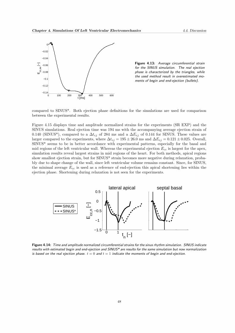
Chapter 4. Simulations Of Left Ventricular Electromechanics 4.4. Discussion

0 100 200 300 400 500 600−0.14

−0.12

−0.1

−0.08

−0.06

−0.04

−0.02

0

t [ms]

Ecc

,av [−

] Figure 4.13: Average circumferential strainfor the SINUS simulation. The real ejectionphase is characterized by the triangles, whilethe used method result in overestimated mo-ments of begin and end-ejection (bullets).

compared to SINUS*. Both ejection phase definitions for the simulations are used for comparisonbetween the experimental results.

Figure 4.15 displays time and amplitude normalized strains for the experiments (SR EXP) and theSINUS simulations. Real ejection time was 194 ms with the accompanying average ejection strain of0.140 (SINUS*), compared to a ∆tej of 284 ms and a ∆Eej of 0.144 for SINUS. These values arelarger compared to the experiments, where ∆tej = 195± 26.0 ms and ∆Eej = 0.121± 0.025. Overall,SINUS* seems to be in better accordance with experimental patterns, especially for the basal andmid regions of the left ventricular wall. Whereas the experimental ejection Ecc is largest for the apex,simulation results reveal largest strains in mid regions of the heart. For both methods, apical regionsshow smallest ejection strain, but for SINUS* strain becomes more negative during relaxation, proba-bly due to shape change of the wall, since left ventricular volume remains constant. Since, for SINUS,the minimal average Ecc is used as a reference of end-ejection this apical shortening lies within theejection phase. Shortening during relaxation is not seen for the experiments.

−1.5

−1

−0.5

0

0.5

Ecc

,n [−

]

tn [−]

SINUSSINUS*

lateral apical septal basal

0 1

Figure 4.14: Time and amplitude normalized circumferential strains for the sinus rhythm simulation. SINUS indicateresults with estimated begin and end-ejection and SINUS* are results for the same simulation but now normalizationis based on the real ejection phase. t = 0 and t = 1 indicate the moments of begin and end-ejection.

48

4.4. Discussion Chapter 4. Simulations Of Left Ventricular Electromechanics

The same observations can be made about the two pacing simulations, as can be observed in figures4.16 and 4.17. Overestimation of the time of ejection leads to different deformation patterns. Totalejection time and amplitude for each simulation is 296 ms and 0.109 (PACEI), 214 ms and 0.101(PACEI*), 284 ms and 0.105 (PACEII), 206 ms and 0.098 (PACEII*), respectively, while for the ex-perimental results ejection time and amplitude is 202.5± 10.6 ms and 0.106± 0.014. From figure 4.16it can be deduced that, except near the apex, influences of wrong estimations are minimal for posteriorand lateral regions both for patterns and amplitude. Mechanical behavior of early and mid activatedregions is not modeled accurate enough. Although the rapid shortening for isovolumic contraction atthe initiation site, fibers are hardly stretched at begin ejection. A reason could be that fiber stiffnessis too high or that the electrical asynchrony between the septal and free wall is not sufficient to causethe mid activated regions to behave abnormal.

Even though endocardial and epicardial asynchrony is increased for PACEII, deformation patterns forboth methods are only comparable for late activated regions, to a certain extent (figure 4.17). Forthe experiments a large increase in lateral apical wall shortening is observed, but this does not holdfor this simulation. Only at the basal septum early stretch at begin ejection is observed, followed byalmost no shortening. One reason for the inaccurate modeling of local deformation in early activatedregions could be that the pacing lead was not exactly positioned at mid septum. This could lead tocomparisons of deformation patterns between the experiments and simulations that are not at the samelocation within the ventricular wall. Furthermore, since no long-axis views are available it is not exactlyknown on what distance from the base the short-axis views are made and can also lead to discrepancies.

Although the model is not capable of a complete reproduction of local deformation, certain phenomenaand trends are comparable between the experiments and simulations. Notably, distributions of timingand total ejection strains as is seen in figures 3.6 and 3.7 for the experiments and figures 4.8 and 4.9for model results. Especially the variation in mean ejection strains are in close proximity: 1.00± 0.25(SR experiments), −1.00 ± 0.05 (SINUS), −1.04 ± 0.76 (pacing experiments), −0.97 ± 0.34 (PACEI)and −0.91 ± 0.88 (PACEII).In figure 4.18 the variation in time to onset and peak shortening as well as the ISF both for SR andpacing results are summarized. Time to onset of and peak shortening is computed with respect tobegin ejection, so differences in timing between the methods is explained by a difference in tbe. Itturned out that time to peak shortening does not depend on ejection phase definition which meansthat the real and estimated begin ejection are in close proximity. Moment of begin ejection for allsimulations is: 38 ms (SINUS), 28 ms (SINUS*), 50 ms (PACEI), 46 ms (PACEI*), 82 ms (PACEII)and 72 ms (PACEII*). Overestimation of total ejection time for SINUS results in a higher ISF, since apart of the isovolumic relaxation phase, where midwall strain slightly rises, is included in the estimatedejection phase. Overall, for both simulations of SR and paced hearts the used method of ejection phasedefinition leads to an increased accuracy of measures of asynchrony compared to experimental results.

49

Chapter 4. Simulations Of Left Ventricular Electromechanics 4.4. Discussion

lateral

base

anterior septal posterior

mid

0 1−1.5

−1

−0.5

0

0.5

apex

tn [−]

Ecc

,n [−

]

SR EXP

SINUSSINUS*

Figure 4.15: Local midwall normalized circumferential strains in time for hearts in SR. Experimental results aredisplayed in black. SINUS represent the strain patterns using the normalization method described in chapter 3.Normalized strains with respect to the real begin and end-ejection is represented by SINUS*. t = 0 and t = 1indicate the moments of begin and end-ejection.

50

4.4. Discussion Chapter 4. Simulations Of Left Ventricular Electromechanics

lateral

base

anterior septal posterior

mid

0 1−2.5−2 −1.5−1 −0.5

0 0.5 1

apex

tn [−]

Ecc

,n [−

]PACEI*PACEI

PACEXP

Figure 4.16: Local midwall normalized circumferential strains in time for paced hearts. Experimental results aredisplayed in black. PACEI represent the strain patterns using the normalization method described in chapter 3.Normalized strains with respect to the real begin and end-ejection is represented by PACEI*.

lateral

base

anterior septal posterior

mid

0 1−2.5−2 −1.5−1 −0.5

0 0.5 1

apex

tn [−]

Ecc

,n [−

]

PACEII*PACEII

PACEXP

Figure 4.17: Local midwall normalized circumferential strains in time for paced hearts. Experimental results aredisplayed in black. PACEII represent the strain patterns using the normalization method described in chapter 3.Normalized strains with respect to the real begin and end-ejection is represented by PACEII*.

51

Chapter 4. Simulations Of Left Ventricular Electromechanics 4.4. Discussion

0

−10

−20

−30

−40

−50

−60

−70

0

−10

−20

−30

−40

−50

−60

−70

0

50

100

150

200

250

300

350

0

50

100

150

200

250

300

350

0

0.05

0.1

0.15

0.2

0

0.05

0.1

0.15

0.2

SHORTENING [ms]TIME TO PEAK

OF SHORTENING [ms]TIME TO ONSET

PACING

ISF [−]

SRE SRS SRS* PE PSI PSI* PSII PSII*

SINUS RHYTHM

Figure 4.18: DMeasures of asynchrony in experimental and simulation results. The first column of SINUS RHYTHMand PACING indicates experimentally obtained values, while the others are simulation results. SRE = SR experi-ments, SRS and SRS* stand for the SINUS simulation, PE = pacing experiments, PSI and PSI* stand for PACEI,PSII and PSII* mean PACEII. The * represents normalized results with respect to real begin and end-ejection.

52

4.4. Discussion Chapter 4. Simulations Of Left Ventricular Electromechanics

4.4.4 Conclusion

The model developed by Kerckhoffs et al. was capable of simulating cardiac electromechanics inseveral conditions. Increasing mechanical asynchrony, induced by high RV septal pacing, led to adecreased pump function and increased variation in timing of onset and peak shortening, ejectionstrain and a larger ISF. However, when the model results were compared with experimental findings,discussed in the previous chapter, it was clear that certain trends and phenomena can be simulatedwell but no perfect reproduction was achieved. On a local scale, mechanical behavior during isovolumiccontraction was similar, i.e. shortening in early activated areas and stretch of the lateral wall. Onthe other hand, for the ejection phase large shortening was observable while stretching septal fibers.But the extent of shortening for lateral fibers was less compared to the experimental findings andseptal stretch was too high. Quantitatively, variations in mean ejection strain, timing and the ISFwere in close proximity. Differences in local deformation patterns might be due to the not optimalprocedure for ejection phase definition which influenced the analysis. Another explanation could bethat variation in strain patterns, especially in early and mid activated regions, differs strongly withinand between animals. Therefore patient specific models are necessary to tune the model parameters.

53

Chapter 4. Simulations Of Left Ventricular Electromechanics 4.4. Discussion

54

Chapter 5

General Discussion

Goal of this study was to test whether the mathematical FE model, developed by Kerckhoffs et al.1,could predict mechanical behavior of healthy and paced hearts. Experimental results of animal stud-ies were used for verification. It turned out that local patterns were not reproduced completely, butgeneral phenomena, such as distributions of timing and total ejection strain were modeled accurately.Several assumptions that were made, such as the active stress-sarcomere length relation and the LVgeometry, might be causes of differences between experimental and model results.

5.1 Active stress - sarcomere length relation

Active stress development is dependent on sarcomere length and the time elapsed since depolarizationas described by equations 4.7 and 4.9. Accidently, the value of parameter a7 was set to 1.7 µm insteadof 1.5 µm. Together with a smaller value of T0 this results in a later start of stress development bythe individual sarcomeres and a lower maximal stress compared to a a7 of 1.5 µm, as presented infigure 5.1. However, a study of Kentish et al.46 revealed that variation in the stress-sarcomere lengthrelation is physiologically feasible and depends on calcium (Ca2+) concentrations. Variation in calciumconcentrations was used before for modeling of mechanical properties of cardiac muscle by Hunter et

al.47. Furthermore, it is hypothesized that the influence of the increased value of a7 is minimal, sincethe isometrical stress development for both values will be comparable as found by van Ooij. He statedthat despite the increase of this value an identical end-ejection stress is found but at a larger minimalsarcomere length. This implies that minimal sarcomere length seems to be defined by a fixed valuefor end-ejection fiber stress.

But since the activation sequence within the heart wall was the only difference between sinus rhythmand pacing conditions and normal behavior is modeled accurately, it still holds that the model iscapable of simulating cardiac mechanics for various conduction settings.

5.2 Interventricular septal motion

The real geometry of the heart, including the RV, is more complex than the truncated ellipsoid weused. Studies from Klima et al.48 and Saleh et al.49 have shown the importance of the interventricularseptum (IVS) on left and right ventricular performance, especially in pathological conditions. Theystate that the IVS functions as the biventricular motor which means that it mediates changes in one

Chapter 5. General Discussion 5.3. Acute vs chronic pacing

1.5 1.6 1.7 1.8 1.9 2 2.1 2.2 2.3 2.4 2.50

20

40

60

80

100

120

140

lc [µm]

f iso [k

Pa]

Figure 5.1: Isometric stress-sarcomere length relations for twovalues of a7 (equation 4.7). Thesolid line represents the stress-sarcomere length relation for a7 =1.5µm, while the dashed line is theused relation and a7 has a value of1.7µm.

ventricle which will subsequently lead to changes in the other ventricle. It is suggested that septal po-sition may determine the magnitude of LV-RV interaction and might affect local deformation patternsin either ventricle.In a normal beating heart the systolic upstroke of left ventricular pressure is slightly earlier comparedto the upstroke of right ventricular pressure. As a consequence, a small movement of the IVS poste-riorly during ventricular ejection was observed after it began to thicken.34 However, when the heartis paced the IVS behaves abnormally. Several explanations for this paradoxical septal motion (PSM)were proposed, including contraction of the RV before the LV, thereby altering the normal transseptalpressure gradient during isovolumic contraction34, early depolarization of the IVS, with septal short-ening unopposed by late depolarized areas50,51 and reversal of the normal direction of septal activationso that it occurs from right to left.A pacing study from Little et al. (1982) stated that PMS was only mediated by this transseptal pres-sure gradient. For all pacing settings (RV apex, RV septal, RV free wall and simultaneous biventricularRV free wall and LV septal pacing), the RV was activated before the LV, causing the right ventricularpressure to increase before left ventricular pressure. The normal left-to-right transseptal gradient wasthereby altered. As a consequence of the unopposed upstroke of the RV pressure, the septum movedtowards the LV. Subsequently, onset of contraction of myofibers in the LV led to a left ventricularpressure rise, exceeding of right ventricular pressure and restoring of the normal pressure gradient andseptal position.Two of the other proposed causes of PSM were modeled during the present study. As is seen infigure 4.5 the initiation site of depolarization is on the right side of the septum and low conductionvelocities results in a right-to-left depolarization wavefront. Findings of the study showed that with-out the load the RV exerts on the LV through RV pressure and force transmission in the IVS it waspossible to produce PSM (figures 4.6 and 4.7), induced by high RV septal pacing. This implies thatintraventricular asynchrony might be more important to develop abnormal behavior of the IVS thaninterventricular asynchrony. But since a deterioration of septal function results in a decrease of RVpump function48,49,52 and in turn influences the systemic circulation, it would be better to use a twochamber geometry and incorporate a pulmonary circulation instead of using the truncated rotationallysymmetric ellipsoid.

5.3 Acute vs chronic pacing

Our model simulates the effects of acute high RV septal pacing, while the animals were paced for 16weeks. Electrical asynchrony not only leads to adverse hemodynamic effects, abnormal distributionsof myocardial work and blood flow, but also to structural changes within the heart wall, like asym-metric hypertrophy. There is also evidence that electrical remodeling within the heart occurs, butthe mechanisms of this process remain unclear.53 A study from Jeyaraj et al.53 revealed a locally

56

5.4. LBBB vs high RV septal pacing Chapter 5. General Discussion

dependent change in action potential duration (APD). In early depolarized areas a slight increase ofthe APD was found, while the APD was progressively shortened in cells within several centimetersfrom the pacing site. In contrast, as one might predict, the APD is markedly prolonged at distal sitesto the site of pacing rather than decreased. A prolonged APD indicates a more slowly repolarizationof the individual myocytes. Since at late-activated regions circumferential strains are increased, theyhypothesized that ventricular electrical remodeling is triggered by mechanoelectrical feedback inducedby a change in the cardiac activation sequence.Acutely, all these effects were reversible, because when pacing the same heart at another location itrevealed identical adaptations.53 Nevertheless, on the long term a downregulation of the potassiumcurrents, that are responsible for repolarization was found by Volders et al.54 As a consequence, cal-cium influx is larger, thereby increasing the excitation time of the muscle fibers. Together with anincreased wall mass at late activated regions14 this may result in a considerable increase in strain anda redistribution of myocardial work.For this study, the only implemented compensation for increasing myocardial work is the Frank-Starlingmechanism. The larger the sarcomere length, the more force it can produce. It might well be that thesmaller circumferential strains in the lateral wall of the simulated paced hearts compared to those fromresults of the chronically paced animals (figure 4.17) is a result of the absence of implemented electricalremodeling. Quantitatively, it might therefore not be straightforward to compare experimental andsimulation results.

5.4 LBBB vs high RV septal pacing

Van Ooij simulated LBBB with the same finite element model developed by Kerckhoffs. Despite sim-ilar activation patterns between LBBB and high RV septal pacing, model results between the twostudies were different. Although local strain patterns of early depolarized regions revealed shorteningand fibers in late activated regions lengthening during isovolumic contraction, no septal stretch andPMS was found at ejection and relaxation for this LBBB study. Because of almost no mechanicalasynchrony, LV hemodynamics was almost equal to cardiac function of a normal heart. Even forPACEI where the same conduction velocities were used, except for the epicardial septum, resultedin different behavior. It might be due to adaptations of the model with respect to van Ooij, whichinclude LV dimensions, active stress behavior, and the impulse initiation site.Left ventricular cavity and wall volume during this study were 35 ml and 90 ml, respectively, comparedwith 44 ml and 136 ml for van Ooij. Moreover, LV dimensions were scaled to preserve the same focaldistance and base-equator length. The reference volume fractions (Vw/Vlv) between the two geometrieswere 2.6 for this study and 3.1 for van Ooij. This decrease in wall mass might lead to a decrease inEF since the ratio is related to ventricular pressure according to Bovendeerd et al.55. A thicker wallis able to produce a larger force, hence more blood can be pumped into the systemic circulation.The second adaptation had to do with the active stress behavior. Because all animals were anes-thetized, contractility will decline and this was modeled by lowering the maximal active stress thatsarcomeres can develop (T0, equation 4.7). For this study a T0 of 150 kPa was used while van Ooijused a T0 of 180 kPa. Although wall mass and T0 were decreased, the model was capable of simulatinghealthy hearts resulting in a EF of 52%, which was also found for the animals of this study. Thereforeit is not likely that these two adaptations alone led to different model results between pacing andLBBB.Another important assumption was decreasing the time constants which regulate stress rate, namelyτr and τd, with 20% (equation 4.9). As a consequence, fiber stress rate was increased. Early activatedfibers shorten faster, stretching lateral fibers to a larger extent compared with van Ooij. But due tothe Frank-Starling mechanism, late activated fibers are able to produce more power, hence ventricularpressure should rise as well.After running a pacing simulation with the values for T0, τr and τd van Ooij had implemented butwith a7 = 1.7µm, it turned out that hemodynamics were slightly better. The SV was increased with1.4 ml and maximal ejection pressure with 0.5 kPa.

57

Chapter 5. General Discussion 5.5. RV apex pacing vs high RV septal pacing

Other possible explanations for these differences could be the initiation site and epicardial septalconduction velocities, since intraventricular delay determines mechanical asynchrony. During LBBBintrinsic conduction of the RV is responsible for left ventricular impulse initiation near the LV apex atthe septal side. Van Ooij assumed fast epicardial septal conduction because the RV is still activatedthrough the right bundle branch and Purkinje system, ending at the right ventricular endocardium.On the other hand, for PACEI and PACEII the pacing lead was positioned near the septal base. Sincethe animals had suffered from a total AV block the impulse was spread through the slow conductingmyocardium only. Because no experimental data was found about conduction velocities of the left sideof the IVS they were made identical to the rest of the epicardial wall. However, it might well be thatendocardial velocities for both ventricles are the same and might influence mechanical behavior.The only major difference between depolarization between this study and LBBB are the direction ofactivation wavefronts within the septum. For LBBB the initial direction is from apex to base but assoon as the wave reaches the endocardium fast propagation occurs. The opposite direction is foundfor PACEI as is displayed in figure 4.5. Total activation time for both studies was approximately70-75 ms, with a relative homogeneous endocardial activation (∼30 ms). So the influence of slowepicardial septal conduction is minimal. Latest activated regions for both studies were the epicardialbasal posterolateral regions. Minimal differences in total activation times and last activated regionscannot be the cause of hemodynamic declination. To test this, another simulation has been performed,but now for a LBBB heart. Identical conduction velocities and active stress behavior as van Ooij wasused with the scaled geometry explained above. Surprisingly, mechanical behavior and accompanyinghemodynamics was almost equal to PACEI. Overall, differences between the two studies must be acombination of geometry, active stress behavior and the site of impulse initiation.

5.5 RV apex pacing vs high RV septal pacing

This paragraph will compare results obtained by Kerckhoffs et al. (2005) who simulated RV apexpacing with the same model with results of both PACEI and PACEII simulations. Model differencesinclude fiber orientation, geometry, conduction velocities, active stress behavior, activation site andan open loop vs closed loop configuration. As mentioned earlier in this report, fiber orientation wasdefined by two angles, αh and αt (figure 4.1). Angle distributions throughout the cardiac wall were forKerckhoffs, −50 < αh < 80 and −20 < αt < 10. Work done by Van Ooij35 revealed an inhomogeneousstress distribution in time while using the angles of Kerckhoffs’ study. Therefore the angles werechosen such that stress were uniform throughout the wall. The angles Van Ooij found were in therange of −80 < αh < 90 and −50 < αt < 15. Furthermore, Kerckhoffs used the geometry described inthe previous paragraph. Conduction velocities are summarized in table 5.1 and it is seen that largestdifferences are found in septal velocities. The velocity ratio for the subendocardium and myocardiumare equal, namely asen = 2.5 and am = 1.5.

Active stress behavior was identical to the study of Van Ooij. Finally, the model of Kerchoffs wasonly capable of simulating one cardiac cycle, while in this study a closed loop configuration was used,thereby reaching steady state at the end of all simulations. As a consequence of an open loop system,the transition between filling and isovolumic contraction and from isovolumic contraction to ejectionwere fixed at 1 kPa and 10 kPa, respectively. For the closed-loop system transitions were based onflows and aortic pressures.

His results showed a total electrical activation of 116 ms, while findings of this study resulted in atotal activation time of 74 ms (PACEI) and 132 ms (PACEII). Local circumferential strain patternsof all studies were consistent, i.e. early depolarized regions shorten during isovolumic contraction andwere stretched during ejection and relaxation. However, the amplitudes were different, especially forthe late activated areas. Maximum Ecc for PACEI was around 0.14, for PACEII around 0.16, whileKerckhoffs observed strains with a maximal value of 0.25-0.28. Also, shortening continued in early

58

5.6. Conclusion Chapter 5. General Discussion

relaxation.Myofiber stress-strain relations were similar in shape for early, mid and late activated areas, butamplitudes were considerably different. For all regions the ranges of fiber strain were for Kerckhoffs: -0.1-0.16 (early), -0.05-0.16 (mid) and -0.08-0.21 (late). According to figure 4.11 ranges were for PACEI0.05-0.12 (early), 0.08-0.19 (mid) and 0.05-0.19 (late) and for PACEII 0.0-0.19 (early), 0.05-0.20 (mid)and -0.01-0.21 (late). An explanation for the increased fiber strains might be due to a different valuefor a7. As mentioned earlier in this chapter, end-ejection stress seems independent on this value, butsarcomere length, and this fiber strain will be larger. This figure shows also that midwall myofiberstresses between all the different areas are small in circumferential direction and only differences ofabout 10 kPa was found from base to apex. On the other hand, stress variation between early, midand late regions was about doubled for Kerckhoffs’ results.Because the pressure at begin ejection is fixed at 10 kPa but was around 8 kPa for PACEI and PACEIIand stresses in early activated regions are higher for the results of Kerckhoffs, lateral fibers have toproduce more force to overcome aortic pressure, hence the afterload is increased and SV is consider-ably higher (40 ml (Kerckhoffs), 28.5 ml (PACEI) and 27.5 ml (PACEII)). All these effects are likelydue to different active stress behavior, since stress development not only depends on stretching ofthe individual sarcomeres but als on tension in neighboring fibers. Overall, it can be concluded thatearly, mid and late activated regions, in spite of different impulse initiation sites, behave similarly, butquantitatively there are large deviations, especially for the LV hemodynamics.

Table 5.1: Conduction velocities for the study of Kerckhoffs et al.1 and for PACEII. cfsen, cfm and cfsep the

conduction velocities along the fiber direction for the subendocardium, myocardium and the epicardial septum, re-spectively, ctsen, ctm and ctsep the conduction velocities perpendicular to the fiber direction for the subendocardium,myocardium and epicardial septum, respectively.

Parameter Unit Kerckhoffs PACEII

cfsen m/s 1.2 0.95cfm m/s 0.75 0.68cfsep m/s 1.2 0.68ctsen m/s 0.8 0.64ctm m/s 0.3 0.28ctsep m/s 0.8 0.28

5.6 Conclusion

The findings of this study demonstrate that with a relatively simple three-dimensional model of theLV it was able to describe local electromechanics of the heart for various conditions, including SRand pacing. Differences in mechanical behavior between the two settings were obvious. Electricalasynchrony, induced by high RV septal pacing led to a redistribution of local ejection strain and timingof onset and peak shortening, compared to healthy hearts, with largest strains and timing for lateactivated regions. Local deformation patterns were not reproduced completely, but general phenomena,such as distributions of timing and total ejection strain were in accordance with experimental dataextracted from MRT images.Since RV function is influenced strongly by mechanical asynchrony and in turn influences the systemiccirculations, including the RV and accompanying pulmonary circulation will improve predictions ofmechanical behavior. Future work may also include better understanding of electrical depolarizationand the accompanying mechanics during acute and chronic pacing and the role of the IVS since thispart of the heart is important for both left and right ventricular performance.

59

Appendices 5.6. Conclusion

60

Appendices

A Magnetic Resonance Tagging

A.1 Nuclear Magnetic Resonance

MRI is based on the principles of nuclear magnetic resonance (NMR), a spectroscopic technique usedto obtain microscopic chemical and physical information about molecules. Every atom can be seenas a tiny magnet that has a certain net magnetic moment vector also called spin that can be mul-tiples of +1/2 or -1/2. The number of spins is directly related to the density of atoms within the object.

When placed in an external magnetic field, ~B0, the spin vector aligns itself with the field vector, justlike a normal magnet would. There is a low energy configuration or state where the poles are alignedand a high energy state where the spin vector is the opposite of the external magnetic field vector(figure A.1). At equilibrium the net magnetic vector of a particle lies along this external field vector. Aparticle with a net spin can undergo a transition from the lower to the high energy state by absorptionof a photon of frequency ν (Larmor or resonance frequency). The energy of this photon must exactlymatch the energy difference between these states and is related to ν (equation A.1)56.

E = hν = hγ‖ ~B0‖ (A.1)

with h Planck’s constant, γ the gyromagnetic ratio which is material dependent and ~B0 the appliedexternal magnetic field.

en

erg

y

magnetic field strentgh

Figure A.1: Energy levels of thelow and high state dependent onthe magnetic field strength ( ~B0).A particle can undergo a transitionfrom either state by absorption oremission of a photon of an energythat equals hγ‖ ~B0‖.

Changing the magnetization by exposing the nuclear spin to energy of a frequency equal to the energydifference between the spin states can result in a state of zero net magnetization. After a certain time(T1) this longitudinal magnetization will return to its equilibrium value.

Appendices A. Magnetic Resonance Tagging

The net magnetization vector can also be rotated using a second external field ~B1 resulting in transversemagnetization . Rotation angle of this vector depends on the time (τ) the field ~B1 is applied, itsmagnitude and γ.

θ = 2πγτ‖ ~B1‖ (A.2)

After this field is turned off the net magnetization vector will rotate around the direction of the initiallyapplied external field ~B0 at frequency ν. Due to differences in net magnetization within the objectthe net vector of different particles will rotate with different frequencies resulting in phase differences.The time needed to return to equilibrium of the transverse magnetization is called T2. Two factorscontribute to the decay of transverse magnetization: molecular interactions and variations in ~B0 withinan atom. The combination of these two factors is what actually results in the decay. The combinedtime constant is called T ∗

2 . The relationship between the T2 from molecular processes and that frominhomogeneities in the magnetic field is 1

T∗

2

= 1T2

+ 1T2,inh

. Both T1 and T2 are material properties

indicating that at a certain time magnetization is different between materials.

As transverse magnetization rotates around the direction of the external magnetic field ~B0 it willinduce an electric current through a coil of wire that is placed within the scanner magnet. Due todephasing of the spins the current will decay in time with time constant T ∗

2 . This signal is called afree induction decay (FID) and construction of MR images is based on these signals (figure A.2).

0

Mtr

t

Figure A.2: Relation betweentransverse magnetization (Mtr) intime, also called a free inductiondecay (FID). This signal is the ba-sis of construction of MR images.

A.2 Construction of MR images

Construction of MR images requires several steps. Normally, only a specified region of the object needsto be examined, so slice selection is the first important step. Slice selection is achieved by applying aone-dimensional, linear magnetic field gradient ( ~Gs) in the direction perpendicular to the image planeduring the period that a radio frequency (RF) pulse is applied (figure A.3). An RF pulse inducesstate transitions, thereby changing magnetization. A 90◦ RF pulse applied in the conjunction withthis magnetic field gradient will rotate the proton spins. Because only those spins that are within thedesired region must be rotated, the frequency content of the pulse is limited to a small interval (∆ν).In the Fourier domain a 90◦ rectangular pulse has a sinc shape with highest amplitude at the frequencyof the RF pulse. Due to multiple frequency components of this function, spins with lower and higherfrequencies that are not located within the desired region are also rotated but by lower angles. A solu-tion to this problem is to use a sinc function in time domain leading to a square frequency distribution.

Location of the image plane along the z-axis is defined by the central frequency of the RF pulse. Slicethickness is controlled by two factors: the amplitude of ~Gs and the bandwidth of the RF pulse, i.e.

62

A. Magnetic Resonance Tagging Appendices

the range of frequencies included in the pulse (equation A.3).

∆z =∆ν

γ‖ ~Gs‖(A.3)

If each of the regions of spin was to experience a unique magnetic field it would be able to imagetheir positions. A gradient in magnetization (~Gφ) along one direction of the image plane, called thephase encoding direction, induces differences in magnetic field, experienced by the object resulting infrequency differences (figure A.3). As soon as this pulse is turned off spins are rotating with the same

frequency again but now the phase of each spin at different values of ~B1 is unique. However it is stillimpossible to locate exact positions by only a phase shift because equal phases arise orthogonal to thephase encoding direction. Applying a second magnetic gradient pulse (~Gf ) along the remaining sideof the image plane, the frequency encoding or readout direction, results in a frequency distribution(figure A.3). Every position within the object is now defined with a unique combination of phase andfrequency. The signal component at a particular frequency (position) along the readout axis is thesum of all the vector contributions from a row of spins in the phase encoding direction. During thissecond pulse the MR signal is sampled acquiring Nx data points. Repeating the measurement Ny

times for different values of the phase encoding gradient, yields a matrix of Nx ×Ny amplitude pointsalso called k-space. Decoding this matrix will eventually produce a spatially resolved image. Two di-mensional Fourier transformation of the data matrix yields a frequency spectrum. Each combinationof frequency and phase is related to a position within the object. The Fourier transformed spectrumis then back-projected to produce the image. The total sequence of magnetization, FID sampling,Fourier transformation and decoding forms the basis of all MR imaging modalities.

Figure A.3: A schematic representation of theimage plane(blue) and the three different gradientpulses necessary for modulation. ~B0 the initial ap-plied external magnetic field, ~Gs the slice selec-tion gradient pulse, ~Gφ the phase encoding gradientpulse and ~Gf the frequency encoding gradient pulse.

A.3 Spatial modulation of longitudinal magnetization

The technique to produce SPAMM prior to imaging was introduced by Axel et al. in 1989 and requiresseveral RF pulses separated by magnetic field gradient pulses. Starting from a longitudinal magne-tization ( ~B0), perpendicular to the image plane, the first RF pulse alters the direction resulting intransverse magnetization all with the same phase (figure A.4A-B). When the RF pulse is turned off, agradient pulse, directed along one side of the image plane, produces a spatial modulation of the phaseof the transverse magnetization in the direction of the gradient (figure A.4C). Subsequently, a secondRF pulse, not necessarily with the same flip angle as the first one turns some of the phase-modulatedtransverse magnetization back into longitudinal magnetization. The amplitude of the modulated lon-gitudinal magnetization depends on the strength of the RF pulses and the position along the directionof the gradient pulse (figure A.4D). After spoiling the transverse magnetization, only the modulatedlongitudinal magnetization remains (figure A.4E) resulting in multiple tag lines. These tags are per-pendicular to the direction of the gradient and have a wavelength that is inversely proportional to thestrength and duration of the gradient pulse. After this pulse sequence an image sequence is appliedas described in appendix A.2.

63

Appendices A. Magnetic Resonance Tagging

x

y

z

equilibrium

M0

45 RF pulseo

gradient pulse

45 RF pulseo

Mz

Mz

Mz

Mz

Mz= 0

after spoilingtransversemagnetisation

Mz= 0

A

B

C

D

E

B0

Bz

Bz B

z

Bz

Bz

Bz

Figure A.4: State of magnetization (B) at different times of the tagging pulse sequence. A: The initial magnetizationalong the main magnetic field (z-direction) with magnitude B0. B: Magnetization after the first RF pulse. TheRF pulse has a flip angle θ with phase along the x axis in the rotating frame. C: Spatial modulation of the phaseof the transverse magnetization produced by the gradient pulse. D: Magnetization after the second RF pulse. Inthis case with the same magnitude and flip angle as the first one. Longitudinal magnetization depends on the yposition. E: Difference in magnetization due to relaxation of both longitudinal and transverse magnetization resultsin a production of light and dark bands. (Modified from Kuijer et al.

57)

64

B. Green-Lagrange strains for the test simulation Appendices

B Green-Lagrange strains for the test simulation

The LV wall in the short-axis view is defined by polar coordinates. In vector notation coordinates are~x0 = r0~er0

(φ0) at end-diastole and ~x = r~er(φ) at later time points. The general deformation equationsfrom which the displacement fields for the test simulations can be derived are:

~x = r~er(φ) with

ri = (1 + α)ri,0 (B.1)(

r2 − r2i

)

=(

r20 − r2

i,0

)

⇒ r =√

r20 − r2

i,0 + (1 + α)2r2i,0 (B.2)

φ = φ0 + β

(

r0 − ri,0

re,0 − ri,0

)

(B.3)

Displacement of material points in time leads to deformation of the tissue. Since, the LV wall isdescribed in polar coordinates first a conversion to cartesian coordinates is required. Subsequently,displacements are calculated by subtraction:

ux = x − x0 (B.4)

uy = y − y0 (B.5)

Strain is defined using the Green-Lagrange strain tensor and is defined by:

E =1

2

(

FT · F − I

)

(B.6)

In this case polar coordinates are used: F = (~∇0~x)T with ~∇0 = ~er0

∂∂r0

+~eφ0

r0

∂∂φ0

. Calculation of F isexplained in the next steps.

FT = (~∇0~x) =

(

~er0

∂∂r0

+~eφ0

r0

∂∂φ0

)

r(r0)~er(φ(φ0, r0))

= ~er0

∂r∂r0

~er + ~er0r ∂~er

∂r0+

~eφ0

r0r ∂~er

∂φ0

= ~er0r0

(

r20 − r2

i,0

(

1 − (1 + α)2))

−1

2

~er + ~er0r ∂~er

∂φ∂φ∂r0

+~eφ0

r0r ∂~er

∂φ∂φ∂φ0

= r0

(

r20 − r2

i,0

(

1 − (1 + α)2))

−1

2

~er0~er + Ar~er0

~eφ + rr0

~eφ0~eφ with A = β

re,0−ri,0

The right Cauchy-Green deformation tensor (C), defined as FT · F , becomes

C = r20

(

r20 − r2

i,0

(

1 − (1 + α)2))

−1

~er0~er0

+ (Ar)2~er0~er0

+

+(

rr0

)2

~eφ0~eφ0

+ Ar2

r0~er0

~eφ0+ Ar2

r0~eφ0

~er0

According to equation B.6 and the above derived equation for C the analytical solutions for the strainsare represented by equations B.7-B.9.

Ecc =1

2

(

(

r

r0

)2

− 1

)

=1

2

(

r20 +

(

2α + α2)

r2i,0

r20

− 1

)

(B.7)

Err =1

2

r20

r20 − r2

i,0

(

1 − (1 + α)2) + (Ar)

2− 1

(B.8)

65

Appendices C. Data analysis

Ecr =Ar2

2r0(B.9)

C Data analysis

C.1 Singular value decomposition

Singular value decomposition is a method to check whether extreme peaks are common in all strainsignals. This filtering procedure is based on the assumption that strains are mutually related and canbe decomposed in a limited number of basic time functions, like harmonics in Fourier analysis32. Thestrain signals are stored in a rectangular strain-time matrix (E) with every row the circumferentialstrain in time for a specific sector. Equation C.1 represents the singular value decomposition of thismatrix.

E =

N∑

i=1

siaibTi (C.1)

with N the total number of columns within E, i.e. number of frames, column vectors ai the orthogonaleigenvectors of EE

T , row vectors bTi the orthogonal eigenvectors of E

TE and the scalar si the square

root of the eigenvalue of ET

E, also called the singular value. This equation states that E can uniquelybe expressed in a linear combination of the mutually independent component matrices (aib

Ti ), where

the singular values (si) are the weighting coefficients for the components.

Singular values correspond with the sum of squares attributed to the bTi components in the rows of

matrix E. The sum of squares of the strain matrix is computed according to equation C.2.

M∑

i=1

N∑

j=1

E2ij = s2

1 + s22 + ... + s2

N−1 + s2N with s2

1 > s22 > ... > s2

N−1 > s2N (C.2)

M represents the total number of sectors. With the use of the SVD of the noisy matrix E, componentsassociated with real strains (large si) are separated from those associated with random noise (smallsi) and they are excluded resulting in truncated components (equation C.3).

Et =

L∑

i=1

siaibTi (C.3)

with L the truncation threshold that can have values 1 ≤ L ≤ N . In order to decide which thresholdvalue should be chosen, knowledge about the noise variance is an important factor. Suppose thatevery measurement has a noise variance σ2, than noise variance for all degrees of freedom together isMNσ2. For every excluded singular value the number of independent degrees of freedom will decreaseaccording to MN − (M +N −L)L, thereby decreasing the total noise variance with the same factor32

and, according to equation C.2, the sum of squares. The difference between the observed and expectedresidual sum of squares of the eliminated components could be used as a threshold (equation C.4).

D =N∑

i=L+1

s2i − (MN − (M + N − L) L) σ2 (C.4)

66

C. Data analysis Appendices

Assume that the minimization is optimal, i.e. D = 0 then a relation between the noise variance andthe threshold can be examined. As is displayed in figure C.1 this function declines rapidly for increas-ing included eigenvalues (L). The second derivative of this relation is used for finding the threshold.For a particular value of L, the second derivative of the noise variance will be negative, indicatingthere exists a saddle point. However, this function will never have a saddle point, but due to discretedifferentiation there exists a point where the first derivative will increase again and that value of Lwill be used for truncation. SVD filtering is followed by smoothing the data through convolution. Anexample of a filtered signal by SVD and convolution is displayed in figure C.1.

5 10 15 20 25 30 350

1

2

3

4

5

6

7

8x 10

−3

L

σ2

0 100 200 300 400 500

−0.16

−0.14

−0.12

−0.1

−0.08

−0.06

−0.04

−0.02

0

t [ms]

Ecc

[−]

Figure C.1: Left: Relation between the truncation threshold and the noise variance at the optimal minimization,i.e. D = 0. The black spot illustrates the threshold for maximal noise variance and indicates the number of includedeigenvalues. Right: The original strain signal is displayed as the solid line, the filtered signal by SVD only (L = 22)is represented by a striped line and a combination of SVD and convolution is displayed as the dotted line.

C.2 Estimation of timing parameters

Timing parameters, Tonset and Tpeak are computed by a computer algorithm implemented in Matlab®

(version 7.4.0). The algorithm determines automatically the onset and peak shortening defined as thetime to onset and time to peak shortening.

Time to onset of shortening

The algorithm starts with determination of the indices of all present peaks in each strain signal. Next,the first maximum found will serve as a first guess of the Tonset. Once this guess is available anestimation is performed using a linearized optimization algorithm. The Tonset is determined by fittingthe model described in equation C.5.

F =

{

a0 + a1t t1 ≤ t ≤ T0

a0 + a1T0 + a2(t − T0) T0 < t < tend(C.5)

with a0 an offset, a1 the slope of the upslope region in the signal in case of early pre-stretch, t1 thefirst time point indicating the time of the minimum before the first guess of Tonset, T0 the parameterthat needs to be optimized and tend the last time point of the data used for optimization indicatingthe time halfway the largest strain rate between next minimum and the first guess.

Important boundary conditions are that the minimal number of data points must be at least threeotherwise the matrix to be solved is singular. In case this boundary condition is not satisfied Tonset

will be the first guess. A second boundary condition involves the value of a2 that must be less or equalto zero. Eventually the Tonset is the value T0 that minimizes the residual error. Figure C.2 illustratesthe above mentioned procedure.

67

Appendices C. Data analysis

Time to peak shortening

Time to peak shortening, or Tpeak is defined as the time where maximal shortening occurs. The firstguess would be the minimum after Tonset but in some cases Ecc increases after this minimum. Acriteria based on the amplitude of this upslope region is used. If this increase is less than 0.5% neglectthat minimum and find the next minimum. Determination of the first peak for strain signals thatcontain multiple peaks is not influenced by this procedure. Another problem arises because the nextminimum might be larger. If this is the case neglect this one as well and go back to the previous one.Figure C.2 will provide more information about the definitions.

Figure C.2: Illustration of theused algorithm for timing defini-tions. The black line correspondsto a strain pattern within a septalregion of a paced heart. The redstriped line indicates the data usedfor optimization starting from t1 totend. T0,opt is the time where theerror between the fit and the strainsignal is minimized and marked asTonset. Tpeak is marked at the firstpeak, because the upslope after thefirst minimum is larger than 0.5%.

Tpeak

Tonset

> 0.5%

t1

tend

T0,opt

68

Bibliography

[1] R.C.P. Kerckhoffs, P.H.M. Bovendeerd, J.C.S. Kotte, F.W. Prinzen, K. Smits, and T. Arts.Homogeneity of cardiac contraction despite physiological asynchrony of depolarization: A modelstudy. Annals of Biomedical Engineering, 31:536–547, 2003.

[2] A.C. Guyton and J.E. Hall. Textbook of Medical Physiology. 9th edition, 1996.

[3] R.H. Anderson, S.Y. Ho, K. Redmann, D. Sanchez-Quintana, and P.P. Lunkenheimer. Theanatomical arrangement of the myocardial cells making up the ventricular mass. European Journal

of Cardio-thoraic Surgery, 28:517–525, 2005.

[4] I. Legrice, P. Hunter, A. Young, and B. Smaill. The architecture of the heart: a data-based model.Phil. Trans. R. Soc. Lond., 359:1217–1232, 2001.

[5] D. Durrer, T. v. Dam, G.E. Freud, M.J. Janse, M.D. Meijler, and R.C. Arzbaecher. Totalexcitation of the isolated human heart. Circulation, XLI:899–912, June 1970.

[6] C.R.C. Wyndham, M.K. Meeran, T. Smith, A. Saxena, R.M. Engelman, S. Levitsky, and K.M.Rosen. Epicardial activation of the intact human heart without conduction defect. Circulation,59(1):161–168, 1979.

[7] F.W. Prinzen, C.H. Augustijn, T. Arts, M.A. Allessie, and R.S. Reneman. Redistribution ofmyocardial fiber strain and blood flow by asynchronous activation. Am J Physiol, 259:H300–H308, 1990.

[8] F.W. Prinzen, W.C. Hunter, B.T. Wyman, and E.R. McVeigh. Mapping of regional myocardialstrain and work during ventricular pacing: experimental study using magnetic resonance imagingtagging. J Am Coll Cardiol, 33:1735–1742, 1999.

[9] M.F. v. Oosterhout, F.W. Prinzen, T. Arts, J.J. Schreuder, W.Y. Vanagt, J.P. Cleutjens, andR.S. Reneman. Asynchronous electrical activation induces asymmetrical hypertrophy of the leftventricular wall. Circulation, 98:588–595, 1998.

[10] K. Vernooy, X.A. Verbeek, M. Peschar, H.J. Crijns, T. Arts, R.N. Cornelussen, and F.W. Prinzen.Left bundle branch block induces ventricular remodeling and functional septal hypoperfusion. Eur

Heart J, 26:91–98, 2005.

[11] O. Lindner, J. Vogt, A. Kammeier, P. Wielepp, J. Holzinger, D. Baller, B. Lamp, B. Hansky,R. Korfer, D. Horstkotte, and W. Burchert. Effect of cardiac resynchronization therapy on globaland regional oxygen consumption and myocardial blood flow in patients with non-ischaemic andischaemic cardiomyopathy. Eur Heart J, 26:70–76, 2005.

[12] M.F. v. Oosterhout, T. Arts, J.B. Bassingthwaighte, R.S. Reneman, and F.W. Prinzen. Relationbetween local myocardial growth and blood flow during chronic ventricular pacing. Cardiovasc

Res., 53:831–840, 2002.

[13] F.W. Prinzen, E.C. Cheriex, T. Delhaas, M.F. v. Oosterhout, T. Arts, H.J. Wellens, and R.S.Reneman. Asymmetric thickness of the left ventricular wall resulting from asynchronous electricactivation: a study in dogs with ventricular pacing and in patients with left bundle branch block.Am Heart J, 130:1045–1053, 1995.

[14] K. Vernooy. Dyssynchronopathy and the role of cardiac resynchronization therapy. PhD thesis,Universiteit Maastricht, 2006.

[15] C. Leclercq and D.A. Kass. Retiming the failing heart: principles and current clinical status ofcardiac resynchronization. J Am Coll Cardiol, 39(2):194–201, 2002.

69

[16] W.F. Kerwin, E.H. Botvinick, J.W. O’Connell, S.H. Merrick, T. DeMarco, K. Chatterjee,K. Scheibly, and L.A. Saxon. Ventricular contraction abnormalities in dilated cardiomyopa-thy: effect of biventricular pacing to correct interventricular dyssynchrony. J Am Coll Cardiol,35:1221–1227, 2000.

[17] M. Peschar, H. de Swart, K.J. Michels, R.S. Reneman, and F.W. Prinzen. Left ventricular septaland apex pacing for optimal pump function in canine hearts. J Am Coll Cardiol, 41:1218–1226,2003.

[18] B.M. v. Gelder, F.A. Bracke, A. Meijer, L.J.M. Lakerveld, and N.H.J. Pijls. Effect of optimizingthe vv interval on left ventricular contractility in cardiac resynchronization therapy. Am J Cardiol,93:1500–1503, 2004.

[19] A. Janssen, B. Kirn, F. Bracke, B. v. Gelder, V. Starc, and F.W. Prinzen. Abstract 2016: Myocar-dial internal strain fraction predicts volume response in patients with cardiac resynchronizationtherapy. Circulation, 114:II 405, 2006.

[20] E.A. Zerhouni, D.M. Parish, and W.J. Rogers. Human heart: tagging with mr imaging - a methodfor noninvasive assessment of myocadrial motion. Radiology, 169:59–63, 1988.

[21] T.R. Brown, B.M. Kincaid, and K. Ugurbil. Nmr chemical shift imaging in three dimensions.Proc. NatL Acad. Sci., 79:3523–3526, 1982.

[22] J. Pauly, D. Nishimura, and A. Macovski. A k-space analysis of small-tip-angle excitation. Journal

of Magnetic Resonance, 81:43–56, 1989.

[23] J. Pauly, D. Nishimura, and A. Macovski. A linear class of large-tip-angle selective excitationpulses. Journal of Magnetic Resonance, 82:571–587, 1989.

[24] L. Axel and L. Dougherty. Mr imaging of motion with spatial modulation of magnetization.Radiology, 171:841–845, 1989.

[25] M. Kass, A. Witkin, and D. Terzopoulos. Snakes: active contour models. Int J Comp Vision,1:321–331, 1988.

[26] J.L. Prince and E.R. McVeigh. Motion estimation from tagged mr image sequences. IEEE

Transactions on Medical Imaging, 11:238–249, 1992.

[27] S.N. Gupta and J.L. Prince. On variable brightness optical flow for tagged mri. Inform Processing

Med Imag, pages 323–334, 1995.

[28] N.F. Osman, W.S. Kerwin, E.R. McVeigh, and J.L. Prince. Cardiac motion tracking using cineharmonic phase (harp) magnetic resonance imaging. Magnetic Resonance in Medicine, 42:1048–1060, 1999.

[29] N.F. Osman and J.L. Prince. Angle images for measuring heart motion from tagged mri. Proc.

Int. Conf. Imag. Proc, Chicago, pages 704–708, 1998.

[30] N.F. Osman and J.L. Prince. Direct calculation of 2d components of myocardial strain usingsinusoidal mr tagging. Proc. Int. Conf. Imag. Proc, Chicago, pages 142–152, 1998.

[31] L.M. Rodriguez, J. Leunissen, A. Hoekstra, B.J. Korteling, C. Timmermans J.L. Smeets, M. Vos,M. Daemen, and H.J. Wellens. Transvenous cold mapping and cryoablation of the av node indogs: observations of chronic lesions and comparison to those obtained using radio-frequencyablation. J Cardiovasc Electrophysiol, 9:1055–1061, 1998.

70

[32] A.M.M. Muijtjens, J.M.A. Roos, T.T. Prinzen, A. Hasman, R.S. Reneman, and T. Arts. Noisereduction in estimating cardiac deformation from marker tracks. Am. J. Physiol., 258:599–605,1990.

[33] J.J.M. Zwanenburg. Mapping asynchrony of circumferential shortening inn the human heart with

high temporal resolution MRI tagging. PhD thesis, Vrije Universiteit Amsterdam, 2005.

[34] W.C. Little, R.C. Reeves, J. Arciniegas, R.E. Katholi, and E.W. Rogers. Mechanism of abnormalinterventricular septal motion during delayed left ventricular activation. Circulation, 65:1486–1491, 1982.

[35] P. v. Ooij. Electromechanical behavior of the cardiac left ventricle with left bundle branch block.Master’s thesis, Technische Universiteit Eindhoven, 2007.

[36] S.W.J. Ubbink, P.H.M. Bovendeerd, T. Delhaas, T. Arts, and F.N. v.d. Vosse. Towards model-based analysis of cardiac mr tagging data: Relations between left ventricular shear strain andmyofiber orientation. Medical Image Analysis, 10:632–641, 2006.

[37] P. Colli Franzone and L. Guerri. Mathematical modeling of the excitation process in myocardialtissue: influence of fiber rotation on wavefront propagation and potential field. Mathematical

Biosciences, 101:155–235, 1990.

[38] C.S. Henriquez. Simulation the elctrical behavior of cardiac tissue using the bidomain model.Crit. Rev. Biomed. Eng., 21(1):1–77, 1993.

[39] B.J. v. Nierop. Coupling a finite element model of left ventricular mechanics in a closed looplumped parameter model of circulatory hemodynamics. Technical report, Eindhoven Universityof Technology, 2007.

[40] K.A. Tomlinson. Finite element solution of an eikonal equation for excitation wavefront propa-

gation in ventricular myocardium. PhD thesis, The University of Auckland, 2000.

[41] D.W. Frazier, W. Krassowska, P.S. Chen, P.D. Wolf, N.D. Danieley, W.M. Smith, and R.E.Ideker. Transmural activations and stimulus potentials in three-dimensional anisotropic caninemyocardium. Circ. Res., 63:135–146, 1988.

[42] A.M. Scher, A.C. Young, A.L. Malmghen, and R.R. Paton. Spread of electrical activity throughthe wall of the ventricle. Circ. Res., 1:539–547, 1953.

[43] D.E. Roberts, L.T. Hersh, and A.M. Scher. Influence of cardiac fiber orientation on wavefrontvoltage, conduction velocity, and tissue resistivity in the dog. Circ. Res., 44:701–712, 1979.

[44] S. Baruffi, S. Spaggiari, D. Stilli, E. Musso, and B. Taccardi. The importance of fiber orientationin determining the features of the cardiac electric field. Modern Electrocardiology, pages 89–92,1978.

[45] R.C.P. Kerckhoffs. Depolarization wave and mechanics in the paced heart: Model and experiment.PhD thesis, Technische Universiteit Eindhoven, 2003.

[46] J.C. Kentish, H.E.D.J. ter Keurs, L. Ricciardi, J.J.J. Bucx, and M.I.M. Noble. Comparisonbetween the sarcomere length-force relations of intact and skinned trabeculae from rat rightventricle. Circ. Res., 58:755–768, 1986.

[47] P.J. Hunter, A.D. McCulloch, and H.E.D.J. ter Keurs. Modelling the mechanical properties ofcaridac muscle. Progress in Biophysics and Molecular Biology, 69:289–331, 1998.

71

[48] U.P. Klima, M. Lee, J.L. Guerrero, P.J. LaRaia, R.A. Levine, and G.J. Vlahakes. Determinants ofmaximal right ventricular function: Role of septal shift. J. Thorac. Cardiovasc. Surg., 123:72–80,2002.

[49] S. Saleh, O.J. Liakopoulos, and G.D. Buckberg. The septal motor of biventricular function.European Journal of Cardio-thoraic Surgery, 29:126–138, 2006.

[50] I.G. McDonald. Echocardiographic demonstration of abnormal motion of the interventricularseptum in left bundle branch block. Circulation, 48:272, 1973.

[51] A.S. Abbasi, L.M. Eber, R.N. MacAlpin, and A.A. Kattus. Paradoxical motion of interventricularseptum in left bundle branch block. Circulation, 49:423–427, 1974.

[52] C.A. Clyne, J.S. Alpert, and J.R. Benotti. Interdependence of the left and right ventricles inhealth and disease. American Heart Journal, 117(6), 1989.

[53] D. Jeyaraj, L.D. Wilson, J. Zhong, C. Flask, J.E. Saffitz, I. Deschenes, X. Yu, and D.S. Rosen-baum. Mechanoelectrical feedback as novel mechanism of cardiac electrical remodeling. Circula-

tion, 115:3145–3155, 2007.

[54] P.G.A. Volders, K.R. Sipido, M.A. Vos, R.L.H.M.G. Spatjens, J.D.M. Leunissen, E. Carmeliet,and H.J.J. Wellens. Downregulation of delayed rectifier k+ currents in dogs with chronic completeatrioventricular block and acquired torsades de pointes. Circulation, 100:2455–2461, 1999.

[55] P.H.M. Bovendeerd, P. Borsje, T. Arts, and F. v.d. Vosse. Dependence of intramyocardial pressureand coronary flow on ventricular loading and contractility: a model study. Annals of Biomedical

Engineering, 34(12):1833–1845, 2006.

[56] J.P. Hornak. The basics of MRI. 1996.

[57] J.P.A. Kuijer. Myocardial deformation measured with magnetic resonance tagging. PhD thesis,Vrije Universiteit Amsterdam, 2000.

72

Erratum

Accidently, the left ventricular meshes for the electrical activation and mechanics computations weredifferent for all simulations: wall volume and reference state volume were 136 ml and 44 ml (electri-cal activation) and 90 ml and 35 ml (mechanics), respectively. As a consequence, the depolarizationdistribution serving as input for the mechanics computations was not the real activation pattern. Inorder to determine the influence of the different meshes on the activation pattern and total activationtime, the two meshes were used for solving the eikonal-diffusion equation (equation 4.1). Conductionvelocities for these simulations were identical to velocities for PACEII (table 4.2).The result is displayed in figure D.1 with the used depolarization times on the horizontal axis and thedifference in depolarization times between the used and real geometry of the LV on the vertical axis.From this figure, it is immediately clear that the thinner wall and smaller cavity volume influencesthe pattern of activation. Because of the increased differences towards the late activated regions, itcan be concluded that the intraventricular delay will decrease and will result in different mechanicalbehavior. Late activated regions will be stretched to a smaller extent and will produce less force.Variations in timing, total ejection strain and the ISF might be smaller as well. Furthermore the totalactivation time will be smaller: 122 ms instead of 132 ms for the used geometry. But this will notchange the conclusions since the model will still be able to produce different mechanical behavior forseveral electrical activation sequences.

0 20 40 60 80 100 120 140−15

−10

−5

0

5

10

15

20

25

30

35

tused

[ms]

t used

− t re

al [m

s]

early latemid

Figure D.1: Relationbetween the used elec-trical activation timesand the difference indepolarization betweenthe used and real ge-ometry. Since the dif-ference is increased to-wards the late acti-vated regions, it can beconcluded that the in-traventricular delay willbe decreased.