SSME MAIN COMBUSTION CHAMBER AND

NOZZLE FLOWFIELD ANALYSIS

Final Report, Contract No. NAS8-355 10

CI-FR-0085

Prepared for:

National Aeronautics and Space Administration George C. Marshall Space Flight Center Marshall Space Flight Center, AL 358 12

[NASA-@B- 1788931 SSHE &BIN CCBBUSTIOI H86-3 3654 CBABBEB AND BOZZfE FLOVfIELD BNALPSIS Piaal Report (Cont inuug , I I ~ G ~ ) 43 F CSCZ 21N

Uflclas G3/26 43540

Prepared By: Richard C. Farmer

Ten-See W ang Sheldon 9. Smith Hobeft J. Prozan

CONTINUUM, INC. 47 I5 University Drive, Suite 1 13

Huntsville, AL 353 16-3495

https://ntrs.nasa.gov/search.jsp?R=19860022182 2018-07-10T02:21:31+00:00Z

SSME MAIN COMBU$I"I'ON CHAMBER AND

NOZZLE FLOWFIELD ANALYSIS

Final Report, Contract No. NAS8-35510 Report Number .- CI-FR-0085

Prepared for:

National Aeronautics and Space Administration George C. Marshall Space Flight Center Marshall Space Flight Center, AL 35812

Prepared By: Richard C. Farmer

Ten-See Wang Sheldon D. Smith Robert J. Prozan

CONTINUUM, INC. 4715 University Drive, Suite 118

Huntsville, AL 35816-3495

March 1, 1986

'> .

TABLE OF CONTENTS

..................................................... 1 . Introduction 1

............................................ 2 . Steady Flow Predictions 2

............................................. 2.1 Transonic Solution 2

....................................... 2.2 Inviscid Nozzle Expansions 9

........................................... 2.3 Turbulence Effects 13

.......................................... 2.3.1 Turbulence Models 13

........................ 2.3.2 Turbulent Wall Flow Data and Correlations 14

............................ 2.3.4 Turbulent Flow Calculation Procedure 21 . ........................................ 2.4 Turbulent Nozzle Flows 28

....................................... 2.5 Three-Dimensional Flows 30

......................................... 3 . Transient Flow Predictions 31

................................... 3.1 Head-End Boundary Conditions 31

........................... 3.2 Rapid Start-up and Shut-down Transients 34

............................ 3.3 Slow Start-up and Shut-down Transients 35

.................................................... 4 . Conclusions 37

..................................................... 5 . References 38

TABLES/ FIGURES

....................................... Table 1 Performance Predictions 12

....................................... Table 2 Shear Stress Components 27

.......................... Table 3 Turbulent Nozzle Expansions for the SSME 29

Figure 1

Figure 2

Figure 3

Figure 4

Figure 5

Figure 6

Figure 7

Figure 8

Figure 9

Figure 10

Figure 11

Figure 1 2

Figure 13

Figure 14

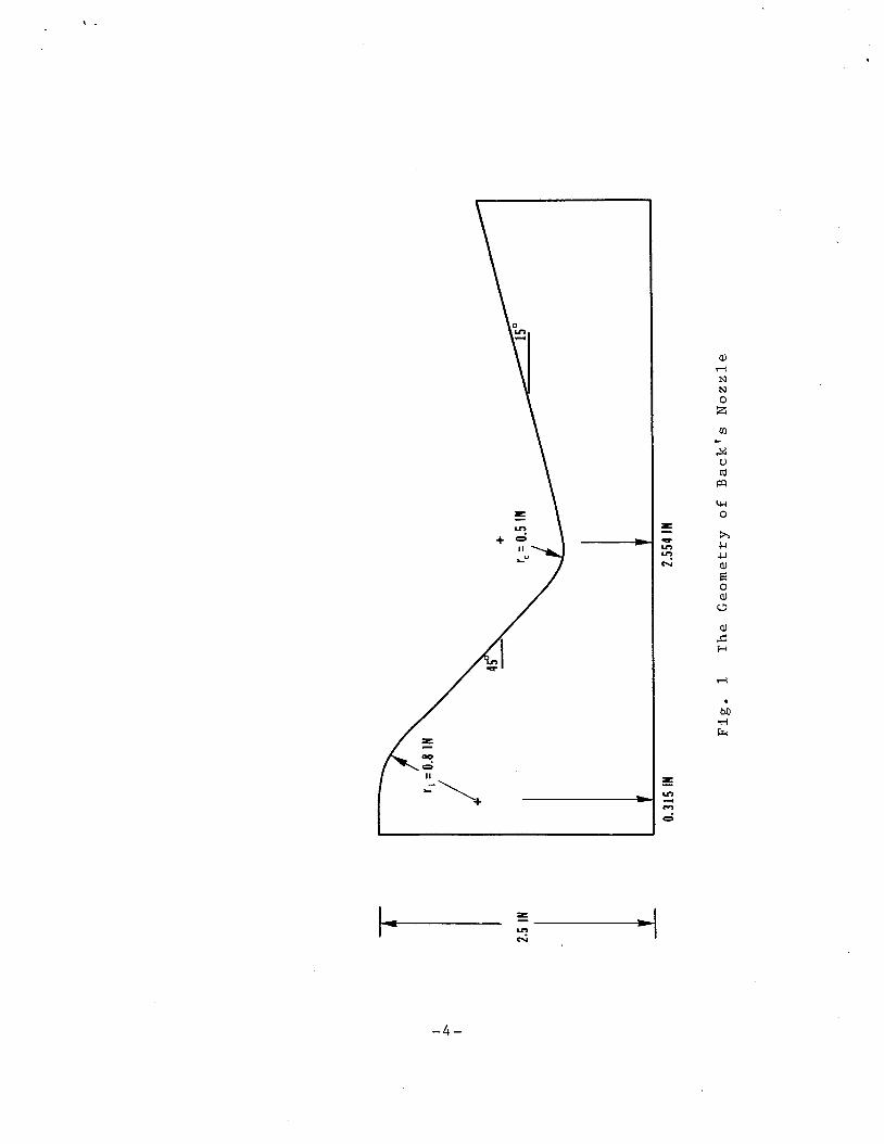
............................... The Geometry of Back's Nozzle 4

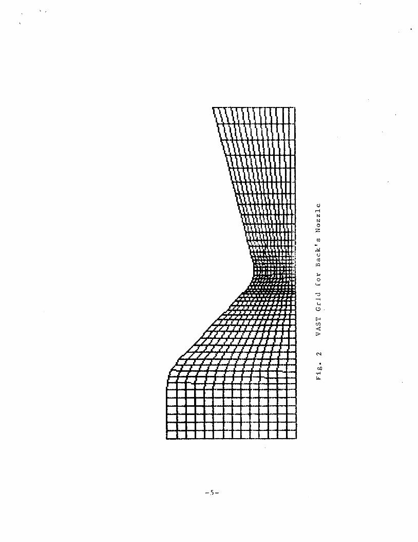
................................. VAST Grid for Back's Nozzle 5

Back's Nozzle Centerline and Wall Static Pressure ............................................. Distribution 7

........................ Back's Nozzle Mach Number Distribution 8

SSME Nozzle Centerline and Wall Static Pressure ............................................. Distribution 10

SSME Nozzle Centerline and Wall Mach Number ............................................ Distribution 11

Semilogarithmic and Linear Plots of Mean Velocity Distribution Across a Turbulent Boundary Layer with .................................... Zero Pressure Gradient 16

...................... Velocity Profiles for Pipes and Flat Plates 17

Musker1s Equation for Velocity as a Function of .................................... Distance from the Wall 18

Eddy Viscosity in Pipe Flow ........................ ? ........ 19

Dim ensionless Shear-Stress Distribution across the Boundary Layer a t Zero Pressure Gradient. according .............................. to the data of Klebanoff (1954) 20

...................... The Correlation Equation for Temperature 24

................. Turbulent Boundary Layer on a Smooth Flat Plate 26

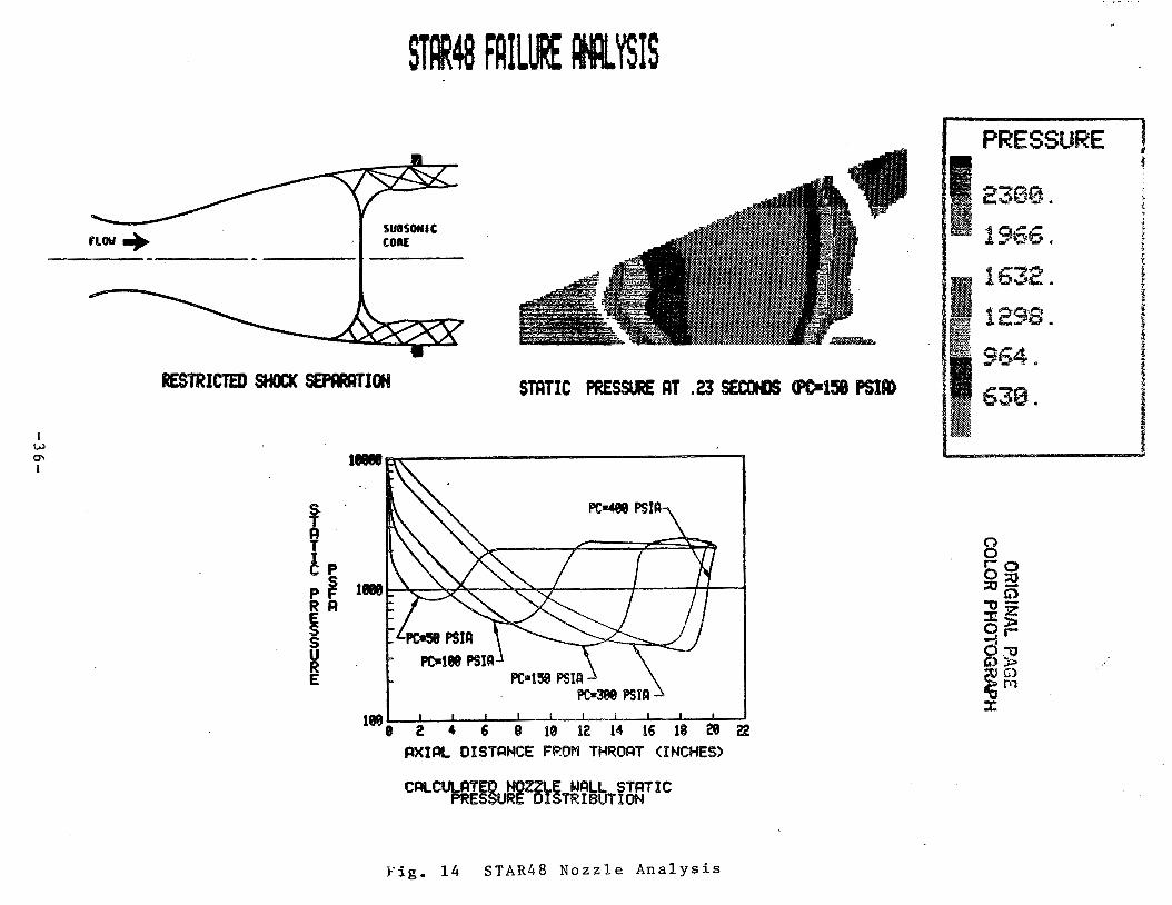
................................... STAR48 Nozzle Analysis 36

CI-F R-00 8 5

1. INTRODUCTION

Steady flow in the main combustion chamber and nozzle of a large axisymmetric rocket

motor, such as the SSME, is generally well understood. Analytical treatments of

transient phenomena have previously been insufficient to quantitatively evaluate

unsteady pressure and heating loads. Three-dimensional steady and transient combustion

chamber/nozzle flows have, in the past, been computationally modeled in a rudimentary

fashion. Performance losses in a rocket engine which are flow related consist of

boundary layer, (both thermal and fricitional), streamline curvature, non-uniform mixture

ratios, and phase and chemical kinetics. All of these phenomena have been isolated for

analytical study. Since the development of Navier-Stokes and turbulence solvers, all of

the flow phenomena may be directly addressed. Furthermore, transient flows may also

be simulated. This investigation is an initial attempt a t unified flow analysis of the gas

dynamics of these flow processes.

Steady operating pressure is reached in about four seconds in the SSME. The relatively

slow chamber pressure buildup in the SSME makes it possible to treat the operation as a

series of quasi steady solutions with variable chamber pressures until steady operating

conditions are reached. A t reduced chamber pressures the nozzle is may be only

partially filled with exhaust gases resulting in a separated flow region between the main

exhaust stream and the nozzle wall. Similar f;9w conditions existed in ground level

static tests of the 5-2, and were the probable cause of the teepee flow structure

observed in those tests.

This research study was an investigation of the computational fluid dynamics tools which

would accurately analyze main combustion chamber and nozzle flow. The importance of

combustion phenomena and local variations in mixture ratio are fully appreciated;

however, the computational aspects of the gas dynamics involved were the sole issues

addressed in this study. The CFD analyses made are first compared with conventional

nozzle analyses to determine the accuracy for steady flows, and then transient analyses

are discussed.

2. STEADY FLOW PREDICTIONS

Steady, axisymmetric flowfield analyses for the flows in liquid rocket engines have been

available for many years (Ref. 1,Z). The direct solution of the governing conservation

equations without making multiple analyses of the various flowfield substructures could

not be accomplished until computers of sufficient size and speed and Navier-

Stokes/turbulent flow solvers were developed. This investigation was an assessment of

Continuum's VAST code (Ref. 3), a Navier-Stokes solver, as a transient model for SSME

main combustion chamber/nozzle flowfield predictions. Boundary condition treatments

and model verifications are presented in this report.

2.1 Transonic Solution

One of the components of the main combustion chamber and nozzle flow analysis is the

combustion chamber and transonic flow analysis. Prior to this contract, the applicability

of the VAST code to mixed (subsonic-transonic-supersonic)internal flows had not been

adequately demonstrated. Thus, the immediate application of the VAST code to the main

combustion chamber-nozzle transonic solution was not undertaken until a validation

calculation was performed. Generally, code validation is performed by comparing a

calculation against either experimental data or an accepted model's calculations. In t h ~

late 60% L. Back (Ref. 4) of Jet Propulsion Laboratory performed an experimental study

of a small throat radius of curvature ratio, converging, diverging nozzle. The

experimental nozzle flowed room temperature air. High resolution data was taken on the

nozzle wall and centerline which provided Mach numbers and static pressure

distributions. Good comparison with this data is considered an important check on any

candidate nozzle analysis.

The geometry of Back's nozzle is shown in Fig. 1. The nozzle is a converging diverging

nozzle with a throat radius of .8 in., a contraction area ratio of 9.76, an expansion area

ratio of 6.6, a 45 deg. inlet angle, a radius of curvature ratio of 1 from the combustion

chamber to inlet and a throat radius of curvature ratio of .625. The problem was set up

using four regions, A total of 780 grid points were used. There were 15 points in the

lateral direction and axially: 1 2 (region I), 1 5 (region 2), 8 (region 3) and 17 (region 4).

The first region extended .6 in. upstream of the entrance to allow the flow to stabilize at

the real entrance. The first region went from -.6 to .881 in. with two segments. The

first segment of region 1 is a straight line from -.6 to .315 having a constant radius of 2.5

inc. The second segment consisted of a .8 in. radius circular arc whose center is a t X=

.315 and K. =6.7. The second region is the inlet to the throat a t - 45 deg., having 15

points axially. Region 3 consists of eight axial points described by a circular arc whose

radius is .5 in. and extends from the - 45 deg. inlet to the 15 deg. conical expansion

section. The center of the circular arc is a t X = 2.554, R = 1.3 and extends for X=2.2 to

2.683. The fourth region is described by a 15 deg. cone extending to an X of 5.6 in.. The

resulting grid is shown in Fig. 2.

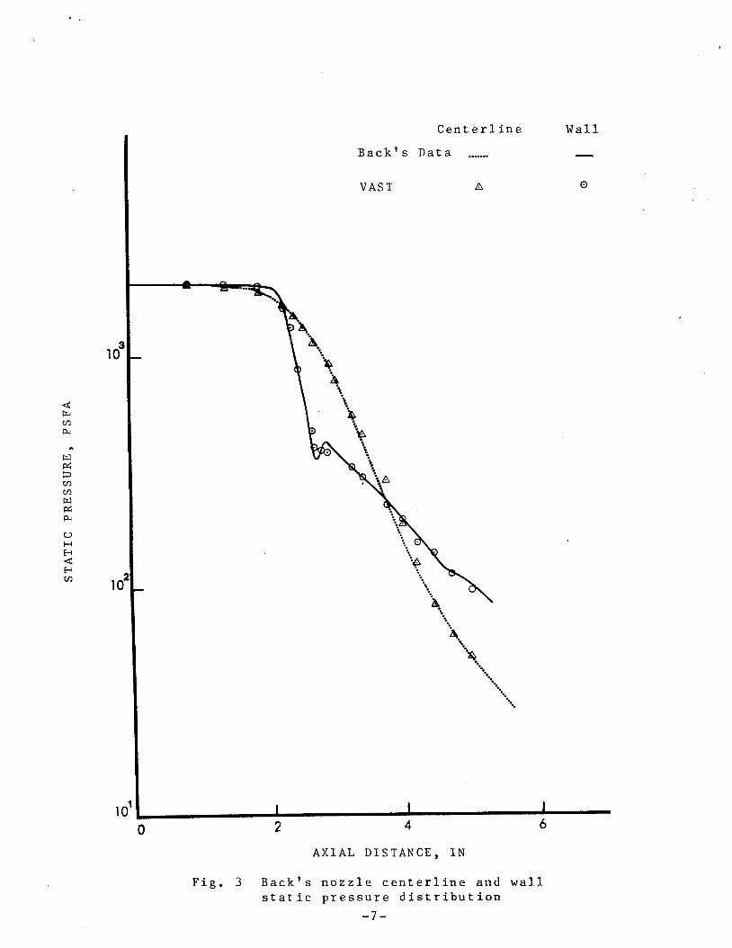
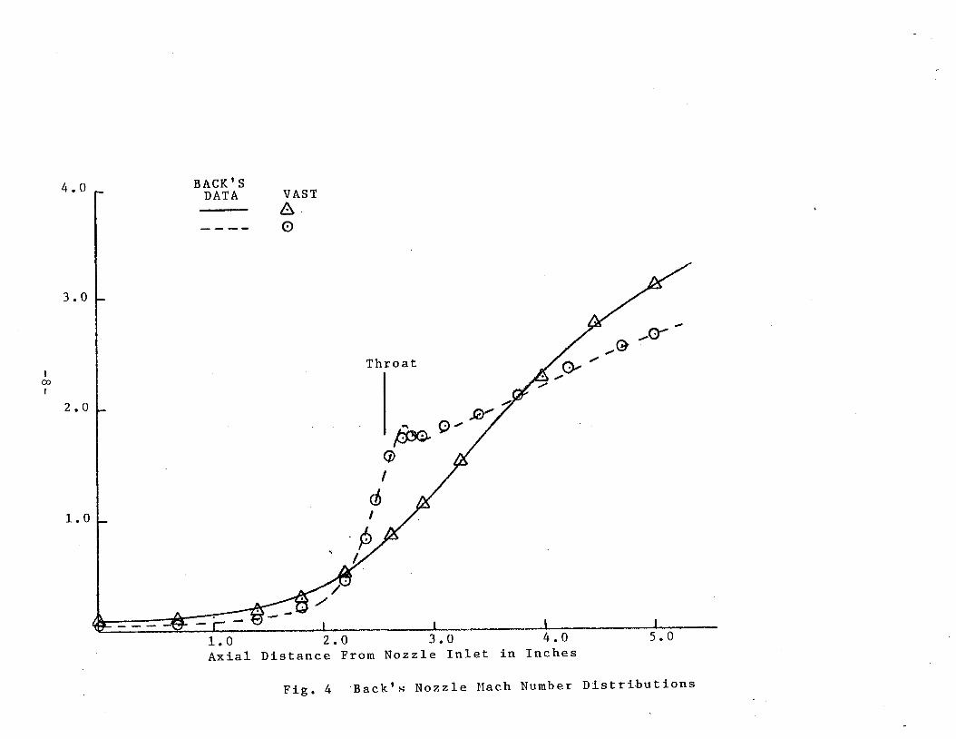
Boundary conditions which were imposed on Back's nozzle were tangency for the

combustion chamber/nozzle wall and axis, free conditions on the exit and total conditions

at the inlet. Total conditions for Back's nozzle were 150.0 psia chamber pressure and 540

R chamber temperature.

The results of the VAST prediction of Back's nozzle are shown in Fig. 3 and 4. Figure 3

presents a comparison of VAST and experimental static pressure distributions along the

combustion chamber/nozzle wall and centerline. Figure 4 presents the same comparison

for Mach number. As can be seen from these two figures, the comparison between VAST

and the data is excellent. The only small deviation occurs a t the recompression region

downstream of the throat. By adding additional grid points in this region, the match

would be much better.

The applicability of the VAST code to solve mixed (subsonic-transonic-supersonic) type

flows which occur in rocket engine combustion chamber and nozzles has been verified

through a comparison with experimental data. The VAST code can now confidently be

used to solve the SSME combustion chamber/nozzle and other liquid rocket engines.

2.2 Inviscid Nozzle Expansions

Expansions in propulsion nozzles are routinely analyzed by using a method of

characteristics (MOC) program followed by a calculation of the nozzle boundary layers

(Ref. 5). The inviscid predictions by the VAST code were tested by comparison to MOC

predictions for ideal gas expansion in the SSME nozzle geometry for a specified sonic line

boundary condition. The results of this investigation are 'reported in this section.

Initial predictions with the VAST code for a relatively crude grid had excellent wall

property comparisons, but failed to predict the rapid centerline expansions known to be

present in the nozzle. The accuracy, as reflected by increasing the grid density, and the

effect of downstream boundary conditions on pressure were investigated as a means of

improving the centerline flow properties. Neither of these effects improved the

predictions. The manifestation of the error was that total pressure deviated from the

known value when the expansion became large, i.e. several orders of magnitude decrease

in static pressure during the expansion. This is a well known problem in using direct

solutions of the Euler equations for nozzle flows, as was recently reconfirmed in (Ref. 6,

7). The VAST code was modified to check and reset the mechanical energy and total

energy at each computation step. Results of these calculations are shown in Figs. 5 and

6. Centerline and wall values of pressure and Mach number are shown to be accurately

predicted for the coarse grid calculation. The VAST code was modified to perform the

integrations required to predic: performance, these results are shown in Table 1. Thrust

was predicted to be within 0.5 percent of the value obtained from the calculation and mass flow a t the exit was calculated to be within 0.2 percent of that specified a t the

throat. The mass flow conservation of the coarse grid VAST calculation is better than

that obtained in the MOC prediction. Since the MOC is a hyperbolic marching solution

while VAST is an elliptic solver, the VAST solution for the steady inviscid nozzle flow

obviously required longer computation time than the MOC solution did. The use of the

constant mechanical energy and total energy creates problems if viscous/turbulent flows

or unsteady flows are considered. These issues are addressed subsequently. In summary,

accurate, steady, inviscid, large expansion nozzle flows are predicted for even coarse-

grid, supersonic nozzle expansions.

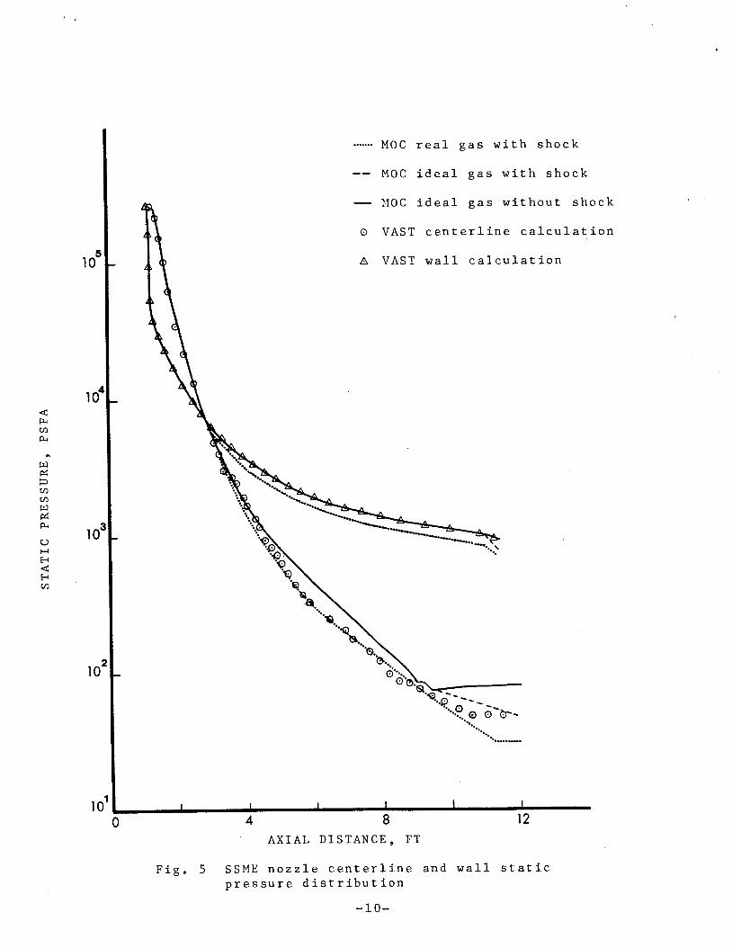
. . . . . . . M O C r e a l g a s w i t h s h o c k

-- M O C i d e a l g a s w i t h s h o c k

- M O C i d e a l g a s w i t h o u t s h o c k

o VAST c e n t e r l i n e c a l c u l a t i o n

A VAST w a l l c a l c u l a t i o n

A X I A L DISTANCE, FT

F i g . 5 SSME n o z z l e c e n t e r l i n e a n d w a l l s t a t i c p r e s s u r e d i s t r i b u t i o n

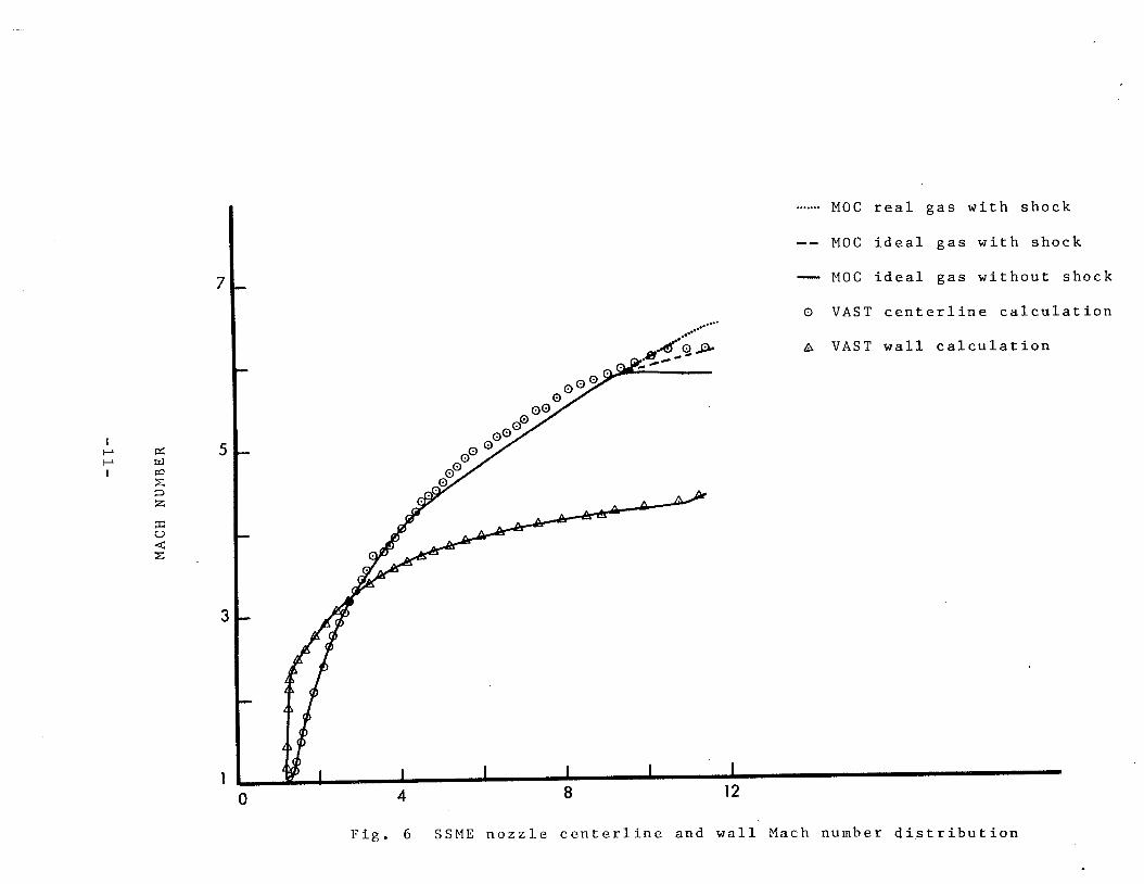
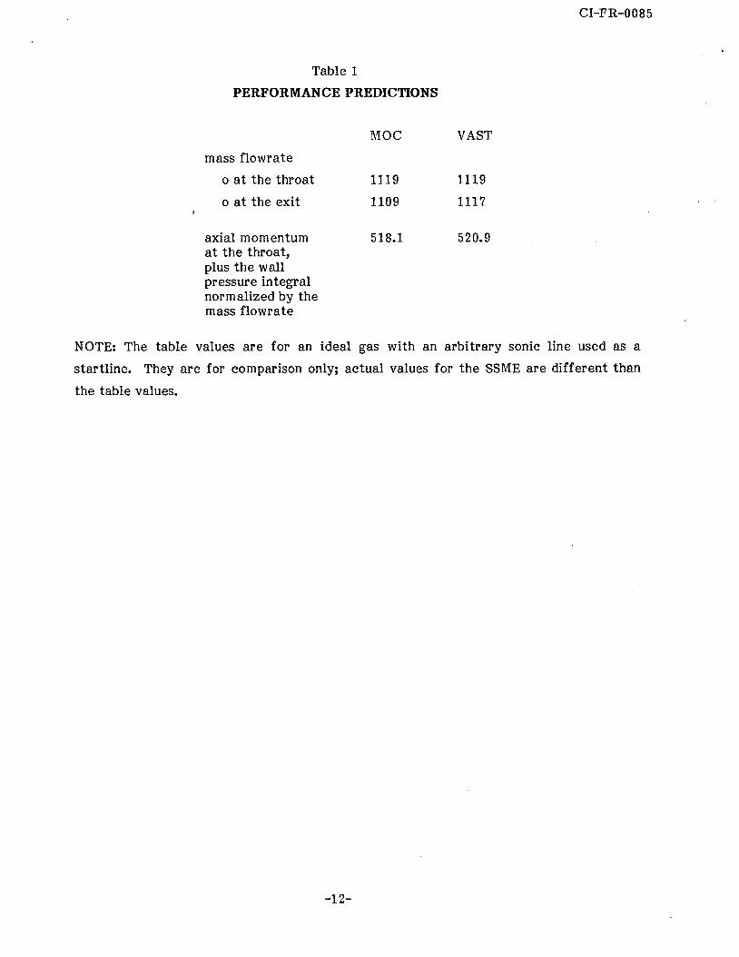
Table 1

PERFORMANCE PREDICTIONS

mass flowrate

o at the throat

o at the exit I

axial momentum at the throat, plus the wall pressure integral normalized by the mass flowrate

VAST

NOTE: The table values are for an ideal gas with an arbitrary sonic line used as a

startline. They are for comparison only; actual values for the SSME are different than

the table values.

2.3 Turbulence Effects

Models to represent the turbulent exchange of momentum and energy must be postulated

to close the time averaged conservation equations. These models should be included in

the calculational procedure. Since the phenomena cannot be predicted from

fundamental principles, either experimental data or analogies to more simple flows must

be used to treat complex turbulent flows like those within the SSME combustion chamber

and nozzle. The time scale for the turbulence averaging is presumed to be less than the

time scale of interest in transient predictions.

2.3.1 Turbulence Models

Turbulent flow causes enhanced mixing and, in some instances, convective-like flow

which is superimposed on an inviscid flow field. Four general types of models are

currently used to represent turbulent flows. The first three of these models start with

the time averaged conservation equations:

1. Algebraic eddy viscosity models.

2. One- and two-equation models.

3. Full Reynolds-stress models.

4. Distribution function models.

For flows in which some of the turbulence scales are much larger than those for other

important flow phenomena, distribution function models have been used. None of these

turbulence models are predictive, all require experimentally determined parameters as

input. Flows over plates and in pipes are the only ones for which even a reasonably

complete data base is available; however, the behavior of turbulence models in predicting

flows around cylinders and over back steps must be reasonable for the models to be

generally useful.

Factors affecting the type of prediction required and/or the geometric and vorticial

complexity of the flow must also enter into the selection of the turbulence model used.

Of necessity the computational algorithm; employed for a given CFD analysis, utilizes a

particular grid density. The selected grid density may require the use of auxiliary

boundary conditions to obtain an accurate solution. These additional boundary conditions

are generally referred to as "wall functions." The nature of wall functions and the

manner in which they are utilized varies greatly from one investigation to another. The

use of wall functions per se does not rule out the possibility of describing heat transfer

effects or flow reversal in zones of separated flow. On the other hand, no general-

purpose, well-established set of wall functions currently exists.

Currently available turbulence data and flow models are summarized and a model for

describing engine related flows is then presented.

2.3.2 Turbulent Wall Flow Data and Correlations

Turbulent flows in smooth pipes and over smooth flat plates have been measured

extensively. Typical data are shown in Fig. 7. Although the velocity changes very

rapidly close to the wall, its variation has been measured. These data are well

represented, piecewise, with the first three equations in Fig. 8 for plates without

pressure gradients and for pipes. Data in the outer region are better fit for plate flow

with pressure gradients by the fourth equation in Fig. 8.

In order to calculate velocity gradients from empirical velocity profiles, it is beneficial

to represent velocity as a continuous function of distance from the wall. Such a

correlation is shown in Fig. 9. Cwrelations for wall shear stress and boundary layer

thickness as functions of free-stream conditions and/or average flow conditions have also

been developed.

The most elementary representation of turbulent flow is to postulate an eddy viscosity by

analogy to laminar viscosity whereby shear stress is determined as the product of eddy

viscosity times the velocity gradient (the Boussinesq approximation). Measurements of

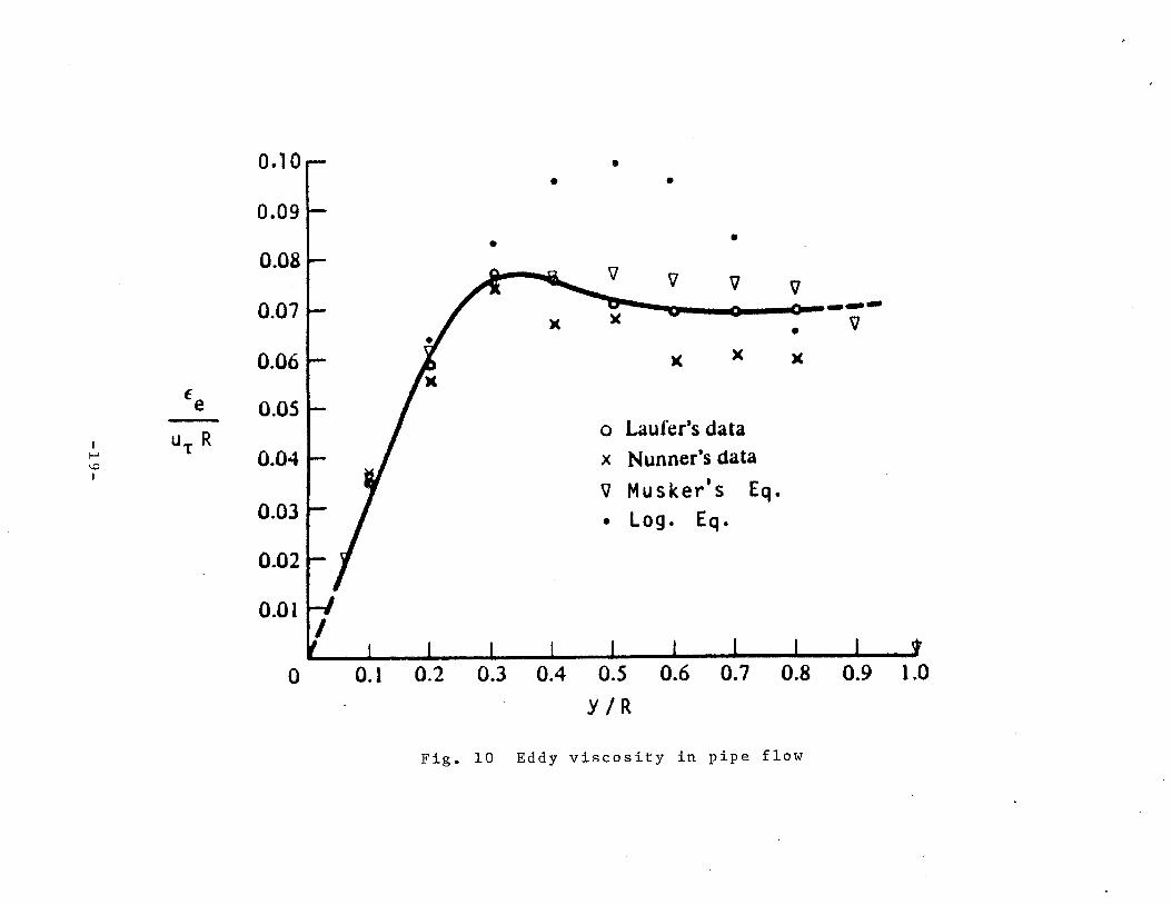
eddy viscosity have been made as shown in Figure 10. To relate eddy viscosity to mean

turbulent flow profies, two new pieces of information are required: the values of shear

stress and of velocity gradient as functions of position from the wall. For fully

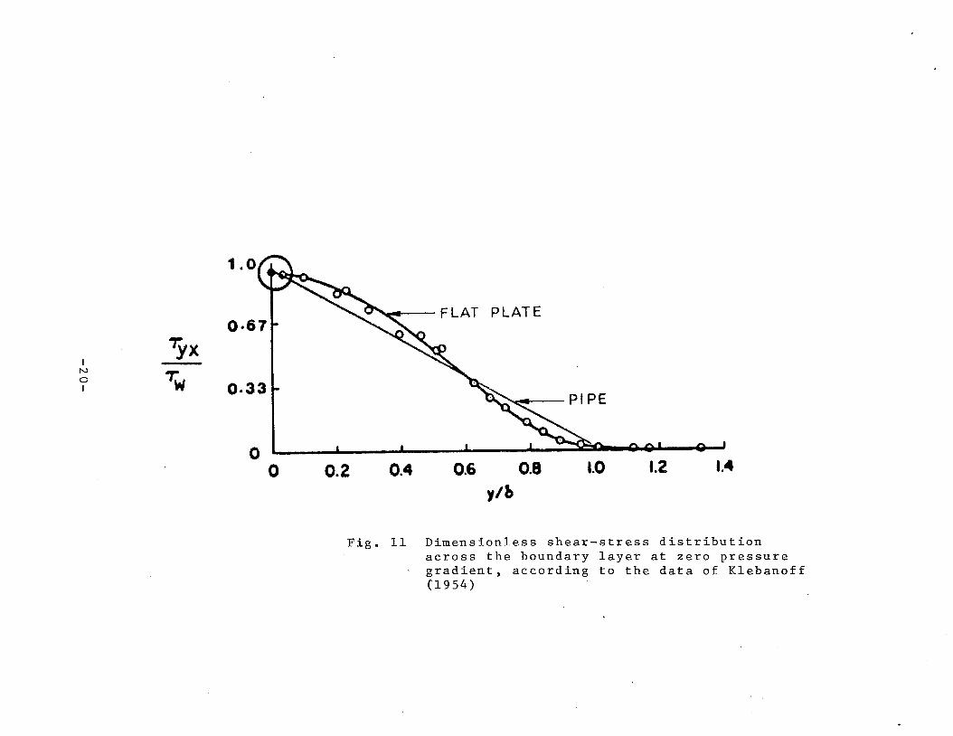
developed pipe flow 'rr = r ( 1 -y/R) . Experimental shear stress data for flow W

over a flat plate are shown in Fig. 11; note the profiles are approximately equal.

Assuming a logarithm etic velocity profile

u = ( u / K ) l n y + c o n s t a n t T

h

&

.rl 0

1-I 0

a)

ri

h

a)

'JJ

d h

'JJ

1-I a)

'JJ fi a

C

w

1

0 0

P

m

4J 4J

0 d

4 a)

ari 1 J-,

M-IP

d

cd

1-Ia

a) 3 -4

d

ud

.rl

'JJ ri

'JJ 1-I M

a m

dm

a

'JJ 0

1-I 1-I

3

0L)m

.rl 'JJ

m

E s

I3 1-I

+.I o a

.rl .r(

M'JO

d

3

1-I M

P

0 'I4

N

ri

$4

.ti

0 C

$ .: 2

ma

3

w

'44 a,

0

h

C

3

(6 C

U

P

om

a,

.rl

aJ ,-I

U

hb

4

5 a

P

w

.rl 0 0

h

$4

ua

cd

r

nN

U

.rl cd

au

a

cd rn

a, rn

UC

a

a,

u

h h

Uc

dO

m

du

I $4

hM

cd

C

a, cd

.rl s

aa

C

OC

h

3

0

mo

o

rn

a o

This value of eddy viscosity is plotted in Fig. 10. Notice that excellent agreement is

obtained for the 30 percent of the flow nearest the wall. If a better velocity profile is

used, a better fit of 1 . 1 ~ should be obtained. Such is the case shown in Fig. 1 0 where

Musl<erls correlation from Fig. 9 is used. The friction velocity, u T , may be evaluated

with a Reynolds-numberlfriction-factor correlation, thusly:

Similar correlations exist for flow over a plate; however, an empirical boundary layer

thickness equation is required as the length scale to replace the pipe diameter.

Recognizing that analyses of more general flows are also required, a computational

technique for the plate and pipe type flows will be developed first. The computational

method thus developed will be used as a starting point for more complex flows.

2.3.4 Turbulent Flow Calculation Procedure

Conceptually, a turbulent flow calculation can be made just like a laminar flow, once an

eddy viscosity model, or other flow model, is specified. However, the very large velocity

gradients near the wall as shown in Fig. 7 indicate that a very fine computational grid

would be required to satisfy a no-slip wall condition and to accurately calculate the sharp

velocity gradients near the wall. To avoid such computational complexity for so small a

region of the flow, a more physical model of the wall region is required. Zero and

modest pressure gradient flows over smooth walls yield time-average velocity profiles

near the wall which are the same. Since the near wall flows are similar, outer flows will

be calculated directly from the solution of the momentum equations and extrapolated

from correlation equations near the wall. The empirical equations will be used to

evaluate the wall shear stress and the shear stress and velocity gradients a t a point

located a yt of 30 (or slightly more). The near wall point is selected to be 30 < y+ < 500

so that the third equation in Fig. 8 and its derivative may be used as the wall functions

for this flow. By assuming negligible flow between the wall and the near wall point, the

exact value of y is immaterial, provided only that y+ remains in the specified bounds.

Computationally, this procedure has proved very acceptable. Had the selection of y

proved to be very sensitive to flow conditions, a more general empirical velocity

correlation, such as Musker's equation, could have been used. To model flows over rough

walls, a modification to the empirical equation is made by defining y+=y/k, and R=8.5

where ks is the roughness height. If the walls are not completely rough,

B = f n ( u T , k s , v) as shown in Schlichting, 7th ed., p. 620 (Ref. 10). If the wall

surfaces were roughened with cut grooves rather than random roughness elements, the ks

and B values would be evaluated by fitting test data. In summary, a method of predicting

momentum exchange in turbulent wall flows has been presented; subsequent discussion

will describe the accuracy of this model.

If empirical temperature correlations were available, all functions could be established

for wall heat transfer. Most attempts to generate temperature correlations have used

turbulent Prandlt numbers; none of these attempts have resulted in even moderately

general correlations. The work of Weigand and Walker (Ref. 11) abandoned the turbulent

Prandlt number concept and produced a useful correlation. Their empirical correlation

contains more parameters than are needed to fit the modest data base which is

available. Physically, the parameters represent streaking and bursting phenomena;

however, if such parameters are approximated to represent the available data base only,

the correlation equation for temperature becomes that shown in Fig. 12.

Conceptually, either qw or Tw can be specified, as either constants or as functions of

position on the surface, to solve a convective heating problem. To complete the solution,

a thermal analysis of the wall is required so that surface heat balances can be made.

Assuming Tw is known, or can be calculated, the solution procedure is to calculate the

temperature gradient normal to the wall by

+ at y + = 3 0 ( = y ) and use this value as the wall function for temperature. If qw is to be specified, K~ and St are calculated from the equations in Fig. 12, then Tw is

calculated for the given qw and the remainder of the calculation procedes as for the

specified Tw case.

A boundary layer calculation was made for the case shown in Fig. 13. The outlet velocity

profile for only 16 nodes in the boundary layer gives a very acceptable solution. A

similar case was run for heating to a cold wall and reasonable temperature profiles were

obtained. Pressure was held constant for the non-isothermal case to stabilize the

solution. In more complex flows, such that the inviscid flow establishes the pressure

field, additional stabilization is not required.

To describe geometrically complex flows, the turbulence models just presented are

generalized by making the following modifications. The time averaged velocities a t

points very near the wall are tangent to the wall for flows with no mass addition. For

flow on a flat plate there is only one significant shear stress component, whereas for

laminar flow in a Cartesian coordinate system all six of the stress components in Table 2

may be important. Since turbulence models for compressible flow have not been well

established, u2 will be assumed zero for turbulent flows. The velocity gradient

determined from the logarithmetic profile described previously will be modified in two

ways in order to evaluate the turbulent counterparts of the stress terms in Table 2.

Symbolically, this gradient is d l v l /dn, where n is along a surface normal direction.

Direction cosines will convert this gradient into components along the coordinate

directions.

Then velocity components will be considered.

Hence, all of the shear stress terms can be evaluated for arbitrarily oriented surfaces.

Velocity and temperature for SSME type nozzle flows were also computed and will be

discussed later in this report.

o 30 n o d e s

+ 16 n o d e s

u ( f t l s e c )

F i g . 1 3 T u r b u l e n t B o u n d a r y L a y e r On A Smooth F l a t P l a t e

Table 2

SHEAR STRESS COMPONENTS

2.4 Turbulent Nozzle Flows

The steady SShlE nozzle flow calculations were repeated for turbulent flow with and

without heat transfer to the nozzle wall. Turbulent nozzle flows have previously been

predicted for the SSME by using the MOC solution and an integral boundary layer

treatment (Ref. 5). These predictions show the boundary layer growing from the head

end of the chamber, through the throat and along the nozzle wall. With the boundary

layer remaining thin in all of these flow passages. The predicted exit plane boundary

layer thickness is about 2 in., for both velocity and temperature.

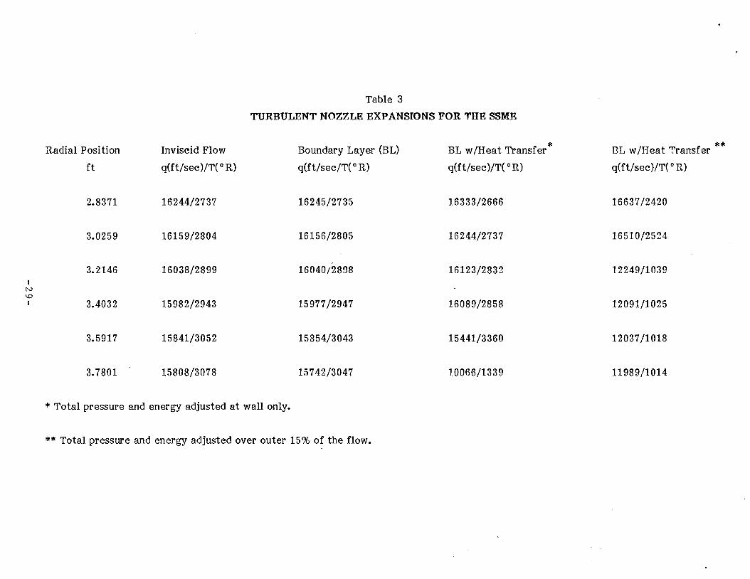
Turbulent flow calculations were made for the SSME nozzle geometry with the

mechanical energy and total energy being held constant at all points, except along the

wall, for the no-heat transfer case. Exit plane profiles of velocity and temperature are

shown in Table 3 for the near wall region. These results show the boundary layer to be

thin; the velocity a t the wall point is the only point significantly affected by the wall.

The distance between the outer two nodes in the exit plane is about 2.5 in.; therefore,

the wall point is the only point which should be significantly influenced by wall friction

or heat transfer. Two sets of calculations were made for the heat transfer case; the first

reset the mechanical energy and total energy a t all except the wall points. Table 3

shows that the predictions look good except for the temperature overshoot a t the next-

to-the-wall point. The second set did not reset the mechanical energy and total energy

otrer the outer 15 percent of the nozzle radius. Table 3 shows that the overshoot is

eliminated, but that thickness of both the velocity and thermal boundary layers are

overpredicted by this set of calculations. A nozzle wall temperature of 1000°R was used

for the heat transfer analyses. Resetting all except the wall points appears to be the

best method of performing turbulent flow calculations, but the practice of holding the

mechanical energy and total energy fixed requires further examination.

CO

tx d'

M

l-l 0

rN

e'

2.5 Three-Dimensional Flows

The VAST code is fully three-dimensional, and all of t h e methodology discussed t o th is

point is equally applicable t o three-dimensional flows. The e f f e c t of including t h e third

dimension t o t h e inviscid calculation merely adds t h e mechanics of solving t h e third

momentum equation. The turbulent flow calculation requires t h a t t h e distance from t h e

wall b e determined fo r each node point. Such a determination must b e made only once

for a problem, but t h e required distances must be s tored in an a r ray which is equal in s i ze

t o t h e number of nodes used in t h e problem.

The three-dimensionality of t h e code has been used extensively in calculating

TAD/manifold/transf e r duc t turbulent flows (Ref. 12). Three-dimensional combustion

chamber and nozzle flows have been calculated by Mr. P. Sulyma, (of MSFC) fo r SRB's.

Duplication of axisymmetric calculations have been made; t h e e f f e c t of nozzle c a n t i s

s t i l l under investigation.

For t h e SSME, non-uniform flow through t h e injector f a c e is t h e major source of three-

dimensionality. Pa ramet r i c analysis of this phenomena is possible with VAST, but

calculations for such a flow were no t made as a p a r t of this study.

3. TRANSIENT PLOW PREDICTIONS

To describe the transient operation of a liquid-propellant rocket motor, the dynamics of

the propellant feed system must be described simultaneously with the flow phenomena in

the main combustion chamber and nozzle. Although a grea t deal is known about t h e

propellant feed systems of operational engines like the SSME, transient simulations of

such systems cannot ye t be modeled to the extent tha t local temperatures, pressures and

flowrates just upstream of the injector face plates can be predicted. Continuum (Ref.

13) has recently provided an orifice type boundary condition for a combustion chamber

which relates local injector mass flowrate t o manifold and chamber pressure.

Anticipating tha t be t te r propellant feed system models will be developed, models t o

represent transient flow in the main combustion chamber will be established.

3.1 Head-End Boundary Conditions

The successful computational anaylsis of the main combustion chamber and nozzle can be

conveniently broken into two main topics: (1) the flowfield analog, and (2) t h e applied

boundary conditions. In this section, we will discuss the l a t t e r topic and, in particular,

the irllet conditions for the motor.

Before discussing the head-end or inlet conditions, let us dispense with all other boundary

conditions which a r e in effect, i.e., the walls and the outlet. The wall boundary

conditions a r e straightforward; involving application of the tangency condition and the

shutting off of an unwanted mass, momentum and energy transfer through the solid

surface. For curved boundaries application of t he tangency condition a t the nodes will

still lead t o apparent flux of conserved quantities through the walls. This tendancy is

eliminated by discarding the apparent flux through the wall in the element integral

calculation. I t is also possible t o achieve flux cancellation by defining the local tangency

a s the chord slope between the surrounding node points. This approach was discarded

since t he local flow angle definition becomes grid dependent.

The outlet boundary condition is more complex. If the steady s t a t e operating condition is

all t ha t is desired and the nozzle flow is supersonic then no boundary conditions, or one-

sided differencing, a re adequate t reatments of the outlet. In t he early stages of start-up

and during shut-down, the surrounding atmosphere must be included in the analysis. That

is to say that the applied boundary condition is far removed from the nozzle exit plane,

rather than at the exit plane.

If enough surrounding atmosphere is included in the analysis, then the downstream

boundary condition becomes simply those atmospheric conditions which exist at the edges

of the computational region during the start-up transient. During shut-down (since the .

plume is very long), a twofold strategy becomes necessary. During the early stages of

shut-down, the plume penetrates the downstream boundary and, as the exhaust gas

production declines, the plume collapses and atmospheric air moves in to occupy the

void. Initially then, the steady state plume drives the downstream boundary and the

condition used is free. After the plume has collapsed, however, we must return to the

atmospheric definition. This process has not been automated and currently is left to the

judgment of the investigator.

During the start-up transient, we must define a sufficiently large atmospheric region

around the exit plane of the nozzle that simply allows the edges to be free. After the

nozzle is flowing full, then the region under investigation may be reduced to simply the

nozzle itself. .

Having dispensed with the relatively straightforward wall and outer boundary conditions,

we now turn our attention to the inlet or head-end conditions. To provide ultra-realistic

transients, it is necessary to model the engine upstream of the combustor to'some deg..

Usually this is so complex that one must settle for a simplified expression for the

manifold pressure upstream of the injectors. A candidate approach is to specify the total

pressure and total temperature downstream of the injectors. If prior testing has yielded

a head-end static pressure (which is generally assumed to be the total pressure, since the

kinetic energy of the propellants is usually negligible), then this information along with

an estimated flame temperature is adequate to perform an analysis of the combustor and

nozzle. This is particularly true a t steady state.

All three options are available in the VAST analysis:

o Analyze in detail the upstream components of the motor.

o Use manifold conditions and approximate orifice pressure drops.

o Use known conditions downstream of the injector.

In the latter two cases, the VAST codes calculate the motion of the independent

variables at the head-end edge of the computational region. Retaining the

instantaneously local value of the pressure (actually, any state variable can be used) and

the instantaneous flow angle, all other required variables can be calculated to enforce

the required condition.

The condition of known total pressure and total temperature downstream of the injector

is then treated in the following fashion:

1. The quantities a t each mode of the upstream edge of the computational zone are

computed a t the end of the nth time step. They are p n , p u n , p vn , p E"

and from these properties the pressure pn is computed.

2. The local flow angle (two-dimensional only is shown for explanatory purposes) is

computed as 8 = tan- ' ( p v n / p u n )

3. From the known total conditions and the local instantaneous pressure, compute

new values of the primary variables:

pGn= bn,/2c ( T ~ - $ " ) s i n 0 P

Where the symbol ( '' ) denotes the adjusted value.

The first two steps are identical where the manif old/orif ice boundary condition

is involved. The steps to compute the adjusted conditions are altered, however.

They are:

, P En are known input values.

And where CI is the local effective discharge coefficient and Sc is the local

orifice flow area locally.

One additional boundary condition is implicit in the analysis a t the throat through the

choking condition. The condition, which corresponds to the maximum mass flow which

the nozzle can pass (at a given initial condition), occurs automatically in the solution of

the field. Once this occurs, the chamber is no longer sensitive to the downstream

boundary condition at the exit of the nozzle, or to any changes in the external field.

These, then, are the conditions which are available and, indeed, must be used to provide a

realistic start-up transient and steady state solution, as well as the shut-down transient,

if desired. It should be pointed out that the head-end conditions may be provided as a

function of time making the entire unsteady solution as good as the known head-end

information.

3.2 Rapid Start-up and Shut-down Transients

For an ideal gas simulation of parallel flow in a cylindrical combustion chamber, the

total conditions and one additional variable must be specified. For steady flow, the

additional variable is determined by the choking condition at the throat to evaluate the

mass flowrate. In the transient solution, however, the mass flowrate of each cross

section is different. A t very early times, for instance, there is flow into the chamber but

no flow through the throat. For liquid-propellant motors, the model postulated in this

analysis is that the total pressure, total temperature, flow angle and static pressure at

the injector are specified functions of time. Continuum has previously reported a

solution obtained in this manner to simulate a J-2s (Ref. 14). Since only the methodology

was demonstrated in that work, unrealistically fast start-up transients were simulated in

order to foreshorten the calculations.

3.3 Slow Start-up and Shut-down Transients

Since the pressure rise rates in the SSME are very low, a series of steady-state solutions

at intermediate pressure levels will adequately describe the nozzle flow. Again,

precautions to apply downstream boundary conditions well away from the computational

region of interest must be exercised. The codes and procedure for this calculation have

been developed but the actual calculations have not been performed. Calculations for a

STAR 48 nozzle have been conducted and are shown in Fig. 14. Notice the large Mach

disc which is predicted.

ORIGINAL PAG

E CO

LOR P

HO

TW

WH

4. CONCLUSIONS

A transient, axisymm etric, two-dimensional and three-dimensional CFD analysis for the

SSME main combustion chamber and nozzle flow was developed. Viscous/turbulence

models were included in the analysis.

A critical feature of CFD methods for nozzle flow with large expansions is the accuracy

with which total pressure is determined. Any CFD method considered for use in

modeling nozzle expansions should be carefully evaluated to determine how accurately

total pressure is predicted. The VAST code with the discussed constraints accurately

predicts total pressure.

Turbulent momentum and heat exchange at the system walls are accurately predicted

with the VAST code. Thermal and momentum boundary layer thicknesses compare well

with MOCIboundary layer models.

Further investigations need to be made to determine the local flow rates through

injectors and the transient head-end boundary conditions appropriate to describing SSME

flows.

CI-F R-00 8 5

5. REFERENCES

1. Farmer, R.C., R.J. Prozan, L.R. McGimsey, A.W. Ratliff, "The Verification of a

Mathematical Model which Represents Large, Liquid Rocket Engine PlumesTT, AIAA

Paper No. 66-650 (June 1966).

2. Pieper, J.L., "Performance Evaluation Methods for Liquid Rocket Thrust

Chambers", Aeroject Co., Report TCER9642:0067 (September 1966).

3. Prozan, R.J., lTHypothesis of a Variational Principle for Compressible Fluid

Mechanics", CI-TR-0086 (March 1985).

4. Back, L., AIAAJ, 5 pp. 2219-2221 (December 1966).

5. Evans, R.M., "Boundary Layer Integral Matrix Procedure", Aerotherm Corp., UM-

75-64 (July 1975).

6. Chan, J.S. and J. A. Freeman, "Throat Chamber Performance using Navier-Stokes

SolutionT1, Lockheed R & D Div, HREC, LMSC-HREC-TRD951729 (December 1984).

',

7. Przekwas, A.J., A.K. Singhal, L.T. Tam, "SSME Thrust Chamber Simulation using

Navier-Stokes Equations1!, CHAM, Inc. CHAM 40703 (October 1984).

8. Cebeci, T. and A.M.O. Smith, Analysis of Turbulent Boundary Layers, Academic

Press, NY (1974).

9. Hinze, J.D., Turbulence, 2nd ed, McGraw-Hill, NY (1975).

10. Schlichting, H., Boundary Layer Theory, 7 th ed, McGraw-Hill, NY (1979).

11. Weigand, G.G. and J.D.A. Walker, in Turbulent Boundary Layers, H.E. Weber, ed,

ASME, NY, pp. 221-235 (June 1979).

12. Anderson, P.G. and R.C. Farmer, l'Calculation of Flow About Posts and Powerhead

Model", Continuum, Inc., Interim Report on NAS8-35506 (December 1985).

13. Wang, T.S. and R.C. Farmer, "Computational Analysis of the SSME Fuel Preburner

Flow", Continuum, Inc., CI-FR-0084 (February 1986).

14. Farmer, R.C., tlIgnition and Combustion Processes: Development of A Transient,

Three-Dimensional Rocket Engine Analysis", Continuum, Inc., Contract NAS8-

35260 (June 1984).