Embed Size (px)
Citation preview

FRIEDRICH-ALEXANDER-UNIVERSITAT ERLANGEN-NURNBERGINSTITUT FUR INFORMATIK (MATHEMATISCHE MASCHINEN UND DATENVERARBEITUNG)
Lehrstuhl fur Informatik 10 (Systemsimulation)
Simulation and Visualization of Fire with the Lattice-Boltzmann Method
Florian Rathgeber
Bachelor Thesis


Simulation and Visualization of Fire with the Lattice-Boltzmann Method
Florian Rathgeber
Bachelor Thesis
Aufgabensteller: Prof. Dr. U. RudeProf. Dr. G. Zeng
Betreuer: M.Sc. K. Iglberger
Bearbeitungszeitraum: 03.01.2009 – 12.05.2009


Erklarung:
Ich versichere, dass ich die Arbeit ohne fremde Hilfe und ohne Benutzung anderer als der an-gegebenen Quellen angefertigt habe und dass die Arbeit in gleicher oder ahnlicher Form nochkeiner anderen Prufungsbehorde vorgelegen hat und von dieser als Teil einer Prufungsleistungangenommen wurde. Alle Ausfuhrungen, die wortlich oder sinngemaß ubernommen wurden, sindals solche gekennzeichnet.
Erlangen, den 12.05.2009 . . . . . . . . . . . . . . . . . . . . . . . . . . . . . . . . .


Abstract
The realistic depiction of fire is a challenge for the disciplines of computational simulation andvisualization alike. As the phenomenon is not fully understood yet, finding a suitable model forthe lifelike simulation of fire is difficult. Therefore, most approaches concentrate on the creationof realistic imagery rather than strict physical accuracy.
This thesis attempts a physically motivated simulation and visualization of freely fed fire.The implementation is based on a model presented in the paper “Simulating Fire With TextureSplats” of Wei et al. Fire and smoke are represented by a cloud of particles that are advectedby a velocity field computed with the Lattice-Boltzmann method (LBM). Combined with theSmagorinsky subgrid correction, the fluid simulation is stable even for turbulent flows. Addition-ally, the LBM provides an easy way to integrate second-order boundary conditions and obstaclesin the flow. In this way, the interaction of the airflow with objects and environmental influenceslike wind can be modeled. A temperature field is added to control the creation of smoke from thefire and buoyancy-induced particle movements. Supplemented with an OpenGL 3D engine, theresults can be immediately visualized in real-time with interactive frame rates, using billboardsas particle representations.
Zusammenfassung
Die realistische Darstellung von Feuer stellt sowohl fur die Disziplin der Computersimulationals auch der Visualisierung eine Herausforderung dar. Da das Phanomen noch nicht vollig ver-standen ist, ist es schwierig ein geeignetes Modell fur die naturgetreue Simulation von Feuerzu finden. Deshalb konzentrieren sich die meisten Ansatze mehr auf die Erzeugung realistischenBildmaterials als auf strikte physikalische Genauigkeit.
Diese Arbeit macht den Versuch einer physikalisch motivierten Simulation und Visualisie-rung von offenem Feuer. Die Implementierung basiert auf einem Modell, das im Paper “Si-mulating Fire With Texture Splats” von Wei et al. vorgestellt wird. Feuer und Rauch werdendurch eine Partikelwolke reprasentiert, die von einem mittels der Lattice-Boltzmann-Methode(LBM) berechneten Geschwindigkeitsfeld getragen wird. In Verbindung mit der SmagorinskySubgitter-Korrektur bleibt die Fluidsimulation selbst fur turbulente Stromungen stabil. Außer-dem ermoglicht die LBM die einfache Einbindung von Randbedingungen zweiter Ordnung undHindernissen im Stromungsfeld. Auf diese Weise kann die Interaktion des Luftstroms mit Objek-ten und Umwelteinflussen wie Wind modelliert werden. Ein zusatzliches Temperaturfeld kontrol-liert die Raucherzeugung durch das Feuer und auftriebsbedingte Partikelbewegungen. Erganztdurch eine 3D-Engine in OpenGL konnen die Ergebnisse direkt in Echtzeit bei interaktivenBildwiederholraten visualisiert werden, wobei Partikel durch sog. billboards dargestellt werden.


Acknowledgments
This thesis was partly written during my stay as an exchange student at the Tongji UniversityShanghai, China, in the winter semester 2008 / 2009. I was admitted as a participant to anexchange program organized by the Lehrstuhl fur Technische Elektronik of Prof. Dr. Dr. RobertWeigel at the Technische Fakultat and received financial support granted by the Dean of theTechnische Fakultat. I want to thank my Chinese host university for accepting me, particularlyProf. Zhibiao Feng, who supported me in all the formalities, and Richard Rose, who was alwaysavailable as a contact person in Erlangen. Further, I want to express my gratitude towardsZuowen Jiang, Zheng Li, and Yufan Qiu for assisting me in admistrative problems during mytime at Tongji University.I would like to thank Prof. Dr. Guosun Zeng and Prof. Dr. Ulrich Rude for offering this thesisto me. Dr. Nils Thurey and Klaus Iglberger gave vital hints on how to develop the topic, manythanks for that. Special thanks go to Klaus Iglberger for his ongoing and very prompt supportdespite the long distance from Erlangen to Shanghai. Finally, I want to thank Thomas Heller,Martin Bauer, and Klaus Sembritzki for helping me out with some tedious C++ issues.

Notation
Quantities with no physical units given are non-dimensional. Whenever necessary, a prime isused to distinguish a physical quantity from a corresponding non-dimensional lattice quantity.The notation follows [Thu07].
fi particle distribution functionfi particle distribution function in inverse direction of fif eqi equilibrium distribution functionf ∗i particle distribution function in post collision statewi equilibrium weighting factorC Smagorinsky constantT temperature [K]ρ′ fluid density [kg/m3]ρ lattice fluid density∆t′ physical time step size [s]∆x′ physical cell size [m]µ′ dynamic viscosity [m Pa/s]ν ′ kinematic viscosity [m2/s]λ relaxation time [s]∆t lattice time step∆x lattice cell sizeν lattice viscosityτ lattice relaxation timeei lattice velocity vectorg gravity acceleration vector [m/s2]u′ physical fluid velocity [m/s]u lattice fluid velocity
Abbreviations
CFD Computational Fluid DynamicsD2Q9 Lattice-Boltzmann model in 2D with 9 velocity directionsD2Q19 Lattice-Boltzmann model in 3D with 19 velocity directionsLB Lattice-BoltzmannLBE Lattice-Boltzmann equationLBM Lattice-Boltzmann methodLGCA Lattice Gas Cellular AutomataNS Navier-Stokes EquationsPDE partial differential equation

Contents
1 Introduction 31.1 A Brief Survey of the History of Fire Simulation . . . . . . . . . . . . . . . . . . . 31.2 Overview . . . . . . . . . . . . . . . . . . . . . . . . . . . . . . . . . . . . . . . . . 4
2 The Lattice-Boltzmann Method 52.1 Introduction to the Lattice-Boltzmann Method . . . . . . . . . . . . . . . . . . . . 52.2 Improved Stability with the Smagorinsky Turbulence Model . . . . . . . . . . . . 92.3 Boundary Treatment . . . . . . . . . . . . . . . . . . . . . . . . . . . . . . . . . . 10
2.3.1 No-slip Boundary Conditions . . . . . . . . . . . . . . . . . . . . . . . . . 102.3.2 Acceleration Boundary Conditions . . . . . . . . . . . . . . . . . . . . . . 102.3.3 Inflow Boundary Conditions . . . . . . . . . . . . . . . . . . . . . . . . . . 102.3.4 Outflow Boundary Conditions . . . . . . . . . . . . . . . . . . . . . . . . . 12
2.4 Obstacles . . . . . . . . . . . . . . . . . . . . . . . . . . . . . . . . . . . . . . . . 122.4.1 Cell-Boundary Aligned Obstacles . . . . . . . . . . . . . . . . . . . . . . . 122.4.2 Curved Boundaries . . . . . . . . . . . . . . . . . . . . . . . . . . . . . . . 13
3 Characteristics of Fire 173.1 A Physical Motivation . . . . . . . . . . . . . . . . . . . . . . . . . . . . . . . . . 173.2 Categorization of Fire . . . . . . . . . . . . . . . . . . . . . . . . . . . . . . . . . 173.3 The Color of Flame . . . . . . . . . . . . . . . . . . . . . . . . . . . . . . . . . . . 183.4 Smoke . . . . . . . . . . . . . . . . . . . . . . . . . . . . . . . . . . . . . . . . . . 20
4 A Model of Freely Fed Fire 214.1 Overview of the Model . . . . . . . . . . . . . . . . . . . . . . . . . . . . . . . . . 214.2 Evaluation . . . . . . . . . . . . . . . . . . . . . . . . . . . . . . . . . . . . . . . . 214.3 Implementation Aspects . . . . . . . . . . . . . . . . . . . . . . . . . . . . . . . . 22
4.3.1 Overview of the Implemented Classes . . . . . . . . . . . . . . . . . . . . . 224.3.2 Particle System Main Loop . . . . . . . . . . . . . . . . . . . . . . . . . . 234.3.3 Particles . . . . . . . . . . . . . . . . . . . . . . . . . . . . . . . . . . . . . 234.3.4 Emission . . . . . . . . . . . . . . . . . . . . . . . . . . . . . . . . . . . . . 234.3.5 Particle Update Step . . . . . . . . . . . . . . . . . . . . . . . . . . . . . . 25
5 Visualization 295.1 Irrlicht 3D Engine . . . . . . . . . . . . . . . . . . . . . . . . . . . . . . . . . . . . 295.2 Particles to the Screen . . . . . . . . . . . . . . . . . . . . . . . . . . . . . . . . . 305.3 Coloring . . . . . . . . . . . . . . . . . . . . . . . . . . . . . . . . . . . . . . . . . 315.4 Environment and Lighting . . . . . . . . . . . . . . . . . . . . . . . . . . . . . . . 325.5 Integration into the Particle System . . . . . . . . . . . . . . . . . . . . . . . . . . 33
6 Performance Aspects 35
XI

6.1 Lattice-Boltzmann Solver . . . . . . . . . . . . . . . . . . . . . . . . . . . . . . . . 356.1.1 Performance Impact of the Smagorinsky Turbulence correction . . . . . . . 356.1.2 Obstacle Boundary Conditions Compared . . . . . . . . . . . . . . . . . . 35
6.2 Particles and Rendering . . . . . . . . . . . . . . . . . . . . . . . . . . . . . . . . 376.3 Dynamic Lighting . . . . . . . . . . . . . . . . . . . . . . . . . . . . . . . . . . . . 41
7 Examples And Results 437.1 The Scene Description . . . . . . . . . . . . . . . . . . . . . . . . . . . . . . . . . 437.2 Example Setups and Visual Results . . . . . . . . . . . . . . . . . . . . . . . . . . 44
7.2.1 Influence of Varying Sprite Number per Particle . . . . . . . . . . . . . . . 447.2.2 Dynamic Lighting . . . . . . . . . . . . . . . . . . . . . . . . . . . . . . . . 457.2.3 Selected Example Scenes . . . . . . . . . . . . . . . . . . . . . . . . . . . . 457.2.4 Evaluation of the Results . . . . . . . . . . . . . . . . . . . . . . . . . . . . 48
8 Conclusion 49
Bibliography 51
XII Simulation and Visualization of Fire with the Lattice-Boltzmann Method

List of Figures
2.1 Discrete velocity directions for D2Q9 and D3Q19 models . . . . . . . . . . . . . . 62.2 Stream and collide step . . . . . . . . . . . . . . . . . . . . . . . . . . . . . . . . . 82.3 Bounce back boundary treatment . . . . . . . . . . . . . . . . . . . . . . . . . . . 112.4 Obstacle with curved boundary in the LBM lattice . . . . . . . . . . . . . . . . . 132.5 Intersection calculation of lattice link and sphere . . . . . . . . . . . . . . . . . . . 142.6 Bounce back behavior depending on the position of the wall . . . . . . . . . . . . 152.7 Pre- and post-moving state of an obstacle . . . . . . . . . . . . . . . . . . . . . . 16
3.1 CIE 1931 chromaticity diagram including the Planckian locus . . . . . . . . . . . 193.2 Black body color spectrum for 1000 - 16000K . . . . . . . . . . . . . . . . . . . . 193.3 Influences directing the movement of smoke particles . . . . . . . . . . . . . . . . 20
4.1 Intersection calculation of lattice link and sphere . . . . . . . . . . . . . . . . . . . 224.2 Composition of the particle movement vector . . . . . . . . . . . . . . . . . . . . . 25
6.1 LBM with and without Smagorinsky turbulence correction . . . . . . . . . . . . . 366.2 Curved boundary obstacle for a sphere of radius 15 . . . . . . . . . . . . . . . . . 366.3 Performance of different boundary conditions for obstacles . . . . . . . . . . . . . 376.4 Computing time comparison of LBM, particle update and rendering . . . . . . . . 386.5 Runtimes of a full simulation time step (1 sprite per particle) . . . . . . . . . . . . 396.6 Runtimes of a full simulation time step (2 sprites per particle) . . . . . . . . . . . 396.7 Runtimes of a full simulation time step (4 sprites per particle) . . . . . . . . . . . 406.8 Runtimes of a full simulation time step (8 sprites per particle) . . . . . . . . . . . 406.9 Rendering time comparison for dynamic lighting turned on and off . . . . . . . . . 41
7.1 Simulation after 100 time steps for different numbers of sprites displayed . . . . . 447.2 A soccer ball shot through a campfire with and without dynamic lighting . . . . . 457.3 A campfire with strong wind from the side . . . . . . . . . . . . . . . . . . . . . . 467.4 Two soccer balls shot through a campfire from different sides . . . . . . . . . . . . 467.5 Three soccer balls shot through a campfire from different sides . . . . . . . . . . . 477.6 A teapot placed on a campfire . . . . . . . . . . . . . . . . . . . . . . . . . . . . . 477.7 A teapot placed on a stove inside a room . . . . . . . . . . . . . . . . . . . . . . . 487.8 A fire calmly burning in a fireplace . . . . . . . . . . . . . . . . . . . . . . . . . . 48
XIII

List of Figures
XIV Simulation and Visualization of Fire with the Lattice-Boltzmann Method

List of Algorithms
2.1 Basic algorithm of the Lattice-Boltzmann Method . . . . . . . . . . . . . . . . . . 92.2 Calculation of the delta value for lattice link intersection with the boundary . . . 15
4.1 Particle system main loop . . . . . . . . . . . . . . . . . . . . . . . . . . . . . . . 234.2 Excerpt from the declaration of the class Particle . . . . . . . . . . . . . . . . . . 244.3 Excerpt from the declaration of the class Emitter . . . . . . . . . . . . . . . . . . . 244.4 Simplified implementation of the particle update method . . . . . . . . . . . . . . 27
5.1 A basic Irrlicht engine example . . . . . . . . . . . . . . . . . . . . . . . . . . . . 305.2 Visualization-enabled particle system main loop . . . . . . . . . . . . . . . . . . . 33
1

List of Algorithms
2 Simulation and Visualization of Fire with the Lattice-Boltzmann Method
1 Introduction
Fire is one of nature’s most exciting yet little understood phenomena that has been fascinatingmankind since the earliest days, long before we had means to effectively create and control it.The dangerous and highly destructive nature of experiments involving fire has made scientificexamination always difficult. Only with the upcoming of computer simulation it was possible toinvestigate fire free of danger and destruction and therefore at much lower cost.
A primary goal of most fire simulations was not only to gain new physical and chemical insight,but also to create realistically looking flame visualizations. In this context, computer graphicsdeveloped methods rousing great interest in the film industry that very much appreciated theseexpanding possibilities of comparatively cheap yet highly flexible special effects. In the following,a short historical survey of approaches to simulate fire is given, followed by an overview of thisthesis.
1.1 A Brief Survey of the History of Fire Simulation
With different goals in mind, a variety of different methods have been developed and appliedfor simulation and visualization of fire. The first attempts were more visualization-orientedrather than targeting physical correctness. An early work is the particle-based system of Reeves[Ree83] used to model the “Genesis bomb” in the film Star Trek II: The Wrath of Khan. Atwo-level hierarchy of particle sources came to use, consisting at the first level of particles thatwere themselves particle systems forming the second level and representing the actual explosions.The realism of particle-based approaches largely depends on the number of particles involved,which in turn is limited by the computing power of the hardware, especially at this time. Adifferent path was taken by Perlin and Hoffert [Per85, PH89], who employed an easy to implementnoise-based method to model fire in two and three dimensions, where turbulent behavior wasachieved by fractal perturbation. This approach lacks the possibility of easily integrating externaleffects, such as wind, the spreading of fire, and furthermore requires a fixed viewpoint position.More recently, King et al. [KCR00] used textured splats for flame visualization, reducing thecomputational complexity compared with particle systems as a comparable visual result can beachieved by a much smaller number of splats. The use of high-resolution textures provides aturbulent appearance of the fire as well as smooth boundaries. Their model, however, does notincorporate interaction with external influences like wind and temperature, leaving the animationrather static.
The group around Ari Kaufman were the first to introduce the Lattice-Boltzmann Methodfor the computation of the flow velocity field advecting fire particles and incorporating theinteractions with external wind forces and the environment. They accelerated the LBM usinggraphics hardware and in the work of Wei et al. [WLMK02] combined this approach withtextured splats as basic display primitives to attain real-time rendering frame rates. Zhao et al.[ZWF+03] expanded this idea by fire front propagation on volumetric data sets. The necessityof creating an isosurface was eliminated by using an enhanced distance field generated by a shell
3

1. Introduction
volume that stores density relations of the voxel neighborhood. This enables the fire front todirectly propagate on a virtual surface related to a given isovalue.
1.2 Overview
The foundation for this thesis lies in the idea of basing fire simulation on a Lattice-Boltzmann-calculated velocity field brought up by the Kaufman group. In particular, the model presented inthe paper “Simulating Fire With Texture Splats” [WLMK02] is implemented as a particle systemon top of a Lattice-Boltzmann solver. This central part is then combined with an OpenGL real-time visualization and a versatile configuration approach using a custom configuration file parser.
First of all, the structure of this thesis subdivided into eight chapters is outlined. After thisintroductory chapter, the basics of the Lattice-Boltzmann Method will be recapitulated, alongwith the presentation of a Smagorinsky turbulence model for enhanced stability. Additionally, theimplementation of different kinds of boundary conditions integrated into the Lattice-Boltzmannsolver, including the accurate treatment of curved boundaries, will be explainded in detail.In Chapter 3, some physically motivated considerations for the modeling of fire will be given,covering smoke and the color of flame. Chapter 4 introduces the model of Wei et al. [WLMK02]for freely fed fire, followed by some details on the implementation of the particle system based onthis model, the central part of the thesis. In the subsequent chapter, the real-time visualization inOpenGL based on the open source 3D engine Irrlicht is presented. Chapter 6 presents selectedperformance results, showing the impact of the different simulation components in terms ofcomputational complexity. A brief overview of how to set up a scene for simulation will be givenin Chapter 7, together with visual results for selected example setups. The last chapter willconclude the thesis and give an outlook on possible extensions.
4 Simulation and Visualization of Fire with the Lattice-Boltzmann Method

2 The Lattice-Boltzmann Method
2.1 Introduction to the Lattice-Boltzmann Method
For more than a decade now, scientists and engineers have a new choice for the numerical simu-lation of fluids that has received constantly increasing attention, the Lattice-Boltzmann Method(LBM). Before that, the principal approach for the computation of the flow of incompressiblefluids in Computational Fluid Dynamics (CFD) had been the numerical solution of the Navier-Stokes Equations (NS). This system of second-order partial differential equations (PDE) for anincompressible fluid consists of the momentum equation
∂u′
∂t+ (u′∇)u′ = − 1
ρ0
∇p+ ν∇2u′ (2.1)
that ensures momentum conservation and the continuity equation
∇ · u′ = 0 (2.2)
that ensures mass conservation [WG00, p. 7]. The flow velocity u′ and the pressure p arethe quantities of interest here, ∇ is the nabla operator, ρ0 is the constant mass density bythe assumption of incompressibility, and ν is the kinematic shear viscosity. The latter twocharacterize the fluid under consideration.
The NS equations can be discretized in space and time by well-known methods such as FiniteDifferences (FD), Finite Elements (FE), or Finite Volumes (FV). Difficulties arise through thenon-linearity of the term (u′∇)u′ in the momentum equation, especially for turbulent flows,where the influence of this term gets strong.
A substantially different, mesoscopic approach was introduced with the Lattice Gas CellularAutomata (LGCA) that were originally proposed by Hardy, de Pazzis and Pomeau in 1973 (HPP-model). An in-depth coverage of the topic can be found in [WG00]. The simulation domain isdivided into a lattice of uniform, discrete cells or lattice sites, where the fluid itself is discretizedas particles. These can only reside at lattice sites, where each cell can host either one particleor be unpopulated, and propagate from cell to cell along associated lattice links.
Collisions occurring when two or more particles propagate to the same cell in the same timestep need to be resolved in a way that conserves mass and momentum. These interactions,involving an exchange of momentum between the colliding particles, are strictly local and onlyinvolve the cell where the collision actually happens. Macroscopic values such as density andvelocity can be obtained by coarse graining, i.e. averaging over a large number of cells, hundredsor probably thousands.
In 1986 Frisch, Hasslacher and Pomeau showed that their proposed hexagonal symmetricLGCA-model (FHP-model) in the macroscopic limit satisfies the Navier-Stokes equations1, whereasthe HPP-model does not due to insufficient isotropy. Still, the LGCA suffered from a number
1The proof can also be found in [WG00]
5

2. The Lattice-Boltzmann Method
Figure 2.1: Discrete velocity directions for D2Q9 and D3Q19 models (image taken from Nils Thurey [Thu07])
of weaknesses, the most prominent being the statistical noise caused by the random particlemovement. An approach to alleviate the problem was the introduction of continuous distribu-tion functions instead of the discrete particles proposed by McNamara and Zanetti in 1988. Thismade coarse graining unnecessary and is regarded as the birth of the Lattice-Boltzmann Method.
The calculation of the distribution functions is based on the Boltzmann Equation
∂f
∂t+ u′∇f = Q (2.3)
with f being the distribution function, u′ the velocity, and Q the collision integral. To adapt tothe lattice, the velocity-space is discretized into a finite number of lattice velocities ui with asso-ciated distribution functions fi and the derivatives are approximated by finite differences. Thecollision integral is approximated by a single-relaxation-time kinetic model, a relaxation towards aMaxwellian equilibrium distribution, know as the Bhatnagar-Gross-Krook-approximation (BGK)[QdL92]. These transformations with all quantities non-dimensionalized finally result in theLattice-Boltzmann Equation (LBE)
fi(x + ei∆t, t+ ∆t)− fi(x, t) = −1
τ(fi − f eqi ) (2.4)
with the discrete distribution values fi(x, t) at a lattice site x at time t, representing the fractionof particles moving in that particular direction, lattice velocities ci, time step ∆t, relaxation timeτ and equilibrium distribution functions f eqi . This linear and first-order equation forms the basisof the LBM.
Several possibilities exist for the discretization of the velocity-space in two and three dimen-sions, the most popular ones being the D2Q9 model in two dimensions and the D3Q19 modelin three dimensions. Both are multi-speed models, i.e. they comprise lattice velocities of differ-ent magnitudes that can be combined to corresponding sub-lattices. Refer to Figure 2.1 for an
6 Simulation and Visualization of Fire with the Lattice-Boltzmann Method

2. The Lattice-Boltzmann Method
illustration of the velocity directions. The D3Q19 lattice velocities are defined as
e0 = (0, 0, 0)
e1,2, e3,4, e5,6 = (±1, 0, 0), (0,±1, 0), (0, 0,±1)
e7,...,10, e11,...,14, e15,...,18 = (±1,±1, 0), (±1, 0,±1), (0,±1,±1).
It is evident that there are three different particle velocities: Velocity 0 for the particles at rest,six directions with unit velocity 1, and twelve directions with velocity
√2. Apart from the D3Q19
model, there are also the D3Q15 and D3Q27 models in three dimensions that introduce a fourthsub-lattice with eight velocities of magnitude
√3. The D3Q15 model lacks the
√2 sub-lattice
in return. But as this gives no stability benefit despite the performance penalty and highermemory requirements of eight additional distribution functions for the D3Q27 model, whereasthe D3Q15 model suffers from anisotropy effects far outweighing the performance gain from thesmaller number of distribution functions, the D3Q19 model is the best choice for most practicalpurposes.
The macroscopic quantities density and velocity relevant for CFD can be computed by sum-mation over the particle distribution functions of a cell as
ρ =∑
fi u =1
ρ
∑eifi. (2.5)
Equilibrium distribution functions represent the stationary state of the fluid, which means thatthe distribution functions remain constant over time but not necessarily that the fluid is at rest.They solely depend on the macroscopic density and velocity and can be computed as
f eqi = wiρ[1 + 3ei · u−3
2u2 +
9
2(ei · u)2] (2.6)
where the equilibrium weighting factors wi give the equilibrium distribution functions for aresting fluid of unit density and for the D3Q19 model are given by
wi = 1/3 for i = 0,
wi = 1/18 for i = 1..6,
wi = 1/36 for i = 7..18.
Usually, the LBE is split into two parts, representing the two steps of computation. Oneis the collision step that accounts for the collisions of particles in a cell by linear relaxing thedistribution functions towards their equilibrium state:
f ∗i (x, t) = fi(x, t)−1
τ[fi(x, t)− ωf eqi ]. (2.7)
The other is the streaming step, where particles stream to adjacent cells according to their latticevelocities
fi(x + ei∆t, t+ ∆t) = f ∗i (x, t). (2.8)
In practice, the lattice cell size and time step are normalized as ∆x/∆t = 1 such that thestreaming step is a simple copy operation. It can be performed in two different ways by going over
Simulation and Visualization of Fire with the Lattice-Boltzmann Method 7
2. The Lattice-Boltzmann Method
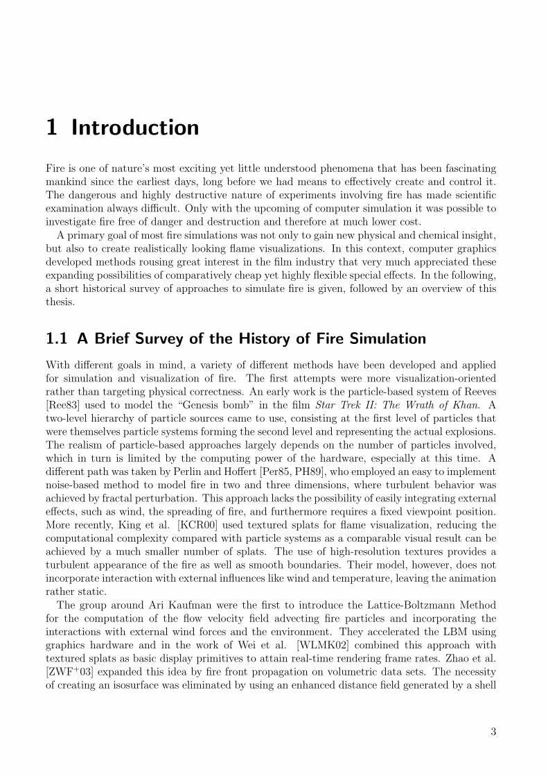
Figure 2.2: Stream and collide step (image taken from Nils Thurey [Thu07])
all lattice cells and either pushing the distribution functions of the current cell to its neighborsor pulling those values from them respectively.
Splitting the LBE as above is referred to as the collide-stream order. Reversing the order tostream-collide as illustrated in Figure 2.2 is perfectly possible as well and numerical differencesbetween the two are negligible. However, [Igl03] attributes the collide-stream order a slightlybetter overall performance. It is common to merge both steps in the implementation to requireonly a single sweep over all grid cells, where in case of the collide-stream order the streamingstep directly pushes to the neighboring cells. As a consequence, the post-collision distributionvalues are never actually stored in the grid. Algorithm 2.1 shows the basic algorithm of theLattice-Boltzmann Method.
8 Simulation and Visualization of Fire with the Lattice-Boltzmann Method

2. The Lattice-Boltzmann Method
1 setup();2
3 for ( int step = 0; step < maxSteps; ++step ) {4
5 collideStream ();6
7 handleBoundaries ();8
9 }
Algorithm 2.1: Basic algorithm of the Lattice-Boltzmann Method
2.2 Improved Stability with the Smagorinsky TurbulenceModel
The Lattice-Boltzmann Method has a limited area of stability that imposes the restriction τ >1/2 on the relaxation time τ , equal to limiting the collision frequency to ω < 2. Stabilityconsiderations for the LBM can be found in [WG00, Chapter 5.6] and [Suc01, Chapter 11.1].The relaxation time τ is related to the kinematic shear viscosity as
ν =2τ − 1
6. (2.9)
As τ approaches 1/2, ν goes to zero and more and more turbulent flow results, correspondingto a high Reynolds number and leading to instability of the basic LBM. Wei et al. [WZF+03]explain this instability with the inability of the LBM to represent flow dynamics on scales smallerthan the lattice spacing, disabling the possibility of energy transfer to these small scales.
To alleviate the issue of the basic LBM becoming more and more unstable, the Smagorinskysub-grid model as described in [HSCD96] and [Thu07] is applied. Sub-grid model in this contextdoes not refer to a grid refinement. Instead it accounts for small-scale physical effects that cannotbe resolved on the ordinary lattice scale by the LBM anymore. This is done by adding a positiveeddy viscosity to the kinematic shear viscosity before the collision step and in turn influencingthe relaxation time τ , pushing it within safe bounds. Consequently, the single-relaxation-timescheme is given up by allowing a variation of the relaxation time over the lattice.
For each cell, a number of local computations need to be done to determine the relaxationtime modification, beginning with the non-equilibrium stress tensor
Πα,β =∑i
eiαeiβ(fi − f eqi ), (2.10)
where α and β run over the three spatial dimensions and i denotes the distribution function orlattice velocity respectively. The second variance of this tensor is given as
Q = Πα,βΠα,β. (2.11)
Next, the intensity of the local stress tensor is computed as
S =1
6C2
(√ν2 + 18C2
√Q− ν
), (2.12)
Simulation and Visualization of Fire with the Lattice-Boltzmann Method 9

2. The Lattice-Boltzmann Method
and finally the modified relaxation time is given by
τs = 3(ν + C2S) +1
2. (2.13)
As S is evidently always positive, the local viscosity is increased proportional to the local stresstensor. Thus, the relaxation time grows alike and is effectively driven out of the critical regionclose to the basis value of 1/2.
2.3 Boundary Treatment
One of the key advantages of the Lattice-Boltzmann Method is the straightforward implemen-tation and natural treatment of boundary conditions. To support flexible setups, it is necessaryto make use of this property and implement different kinds of boundary conditions, as explainedin the following.
2.3.1 No-slip Boundary Conditions
The most commonly used boundary conditions for LBM are the no-slip boundary conditions,representing a “sticky” wall, and characterized by a fluid velocity of zero at the boundary forthe normal as well as the tangential component of the velocity. They are simply implementedas a bounce-back, meaning distribution values that would propagate to a no-slip boundary cellare reversed instead. From an implementation point of view, these values are copied to thedistribution values of the inverse direction as depicted in Figure 2.3. Therefore this condition isoften referred to as “bounce-back” boundary condition of the link bounce back kind that placesthe boundary at the midpoint between fluid and obstacle cell. In terms of implementation itrequires altering the streaming step for every velocity direction i pointing towards a wall to
fi(x + ei∆t, t+ ∆t) = f ∗i (x, t). (2.14)
2.3.2 Acceleration Boundary Conditions
A wall that is not at rest is implemented similar to the no-slip boundary conditions, but thevelocity at the wall is set to a user defined value, the moving speed of the wall, instead of zero.The bounce-back is therefor augmented by a velocity-dependent term, resulting in a streamingstep of
fi(x + ei∆t, t+ ∆t) = f ∗i (x, t) + 6wiρwei · uw (2.15)
where wi is the equilibrium distribution function weighting factor, ρw is the fluid density at thewall and uw is the moving speed of the wall. Frictional forces acted upon the fluid by the wallmovement are modelled by this additional term.
2.3.3 Inflow Boundary Conditions
Fluid flow entering the domain from outside can be modelled by setting the distribution functionsof the inflow boundary cells to the equilibrium distribution values of unit density and a velocity
10 Simulation and Visualization of Fire with the Lattice-Boltzmann Method

2. The Lattice-Boltzmann Method
Figure 2.3: Bounce back boundary treatment (image taken from Nils Thurey [Thu07])
Simulation and Visualization of Fire with the Lattice-Boltzmann Method 11

2. The Lattice-Boltzmann Method
equal to that of the incoming flow specified by the user:
fi(x, t+ ∆t) = wi
(1 + 3ei · uin +
9
2(ei · uin)2 − 3
2(uin · uin)
). (2.16)
2.3.4 Outflow Boundary Conditions
Using the same approach as for an inflow for an outflow boundary condition, where fluid flow issupposed to leave the domain, usually does not give the desired results as the outflow velocity isnot known in advance and thus cannot be pre-defined. What is mostly desired is an outflow withthe current velocity of the cell at the outflow boundary. Feichtinger et al. [FGD+07] suggest twodifferent approaches for that.
The first approach is the pressure boundary condition adapted from [Thu07], where the outflowcells are assigned atmospheric pressure by using the reference density ρA = 1 and setting
fi(x, t+ ∆t) = f eqi (ρA,u) + f eqi
(ρA,u)− fi(x, t) = 2wi
(1− 3
2(u · u) +
9
2(ei · u)2
)− fi(x, t),
(2.17)where u = u(x, t) is the fluid velocity of boundary cell x at time t.
The second approach is imposing a pressure gradient of zero at the boundary by not using aprescribed pressure value like that of the atmosphere, but the current pressure ρ of the cell:
fi(x, t+ ∆t) = 2wi
(ρ− 3
2(u · u) +
9
2(ei · u)2
)− fi(x, t) (2.18)
However, Feichtinger et al. [FGD+07] report that using this second pressure condition as outflowcondition increases the overall domain density when combined with inflow conditions.
2.4 Obstacles
The ease of treating boundary conditions in the Lattice-Boltzmann Method is paired with anequally straightforward way to cope with obstacles in the interior of the flow domain. Twopossibilities are outlined in the following, a very simplistic one for box-shaped obstacles and amore elaborate one handling the curved boundaries of spherical obstacles.
2.4.1 Cell-Boundary Aligned Obstacles
Obstacles in the flow can be easily handled as long as their bounds follow the lattice cell bound-aries by simply defining the corresponding cells as no-slip boundary cells. A cuboid-shapedobstacle is the simplest conceivable case and can be defined by two opposite corner cells. Theirindices delimit the volume to be occupied by the obstacle in the three lattice space dimensions.More complex shapes could be attained by combination of several of these “boxes”.
The standard no-slip boundaries belong to the link bounce back conditions, where the wallis placed exactly halfway between fluid and boundary node. Though this assumption couldbe retained to approximate arbitrary shaped obstacles by the standard no-slip conditions, this“staircase approximation” as described above is not accurate. Figure 2.4(a) shows that for acurved boundary an error is introduced with every bounce back from a link where the wall is
12 Simulation and Visualization of Fire with the Lattice-Boltzmann Method

2. The Lattice-Boltzmann Method
(a) Error introduced by “staircase approximation” (b) Lattice link intersections of a curved boundary
Figure 2.4: Obstacle with curved boundary in the LBM lattice (images taken from Klaus Iglberger [Igl05])
not placed exactly in between two nodes. Thus it is necessary to introduce an appropriate andaccurate treatment for obstacles of more complex shape, for instance curved surfaces like thoseof spheres.
2.4.2 Curved Boundaries
For obstacles of arbitrary shape, the intersection of the obstacle surface with the lattice link canbe at an arbitrary distance between 0 and the link length from the fluid node under consideration.Note that for multispeed models lattice links can be of different lengths such as 1 and
√2 for
the D3Q19 model used. An accurate boundary treatment requires precisely calculating thisdistance that will be referred to as delta value of that particular lattice link or “fluid fraction”.As illustrated in Figure 2.4(b) it represents the fraction of the link length lying within the fluiddomain and is computed as
∆ =|xf − xw||xf − xo|
, (2.19)
with xf being the fluid node and xo the boundary node associated with the link and xw beingthe intersection point with the surface. This fraction needs to be calculated for each lattice linkintersecting the obstacle surface.
Prerequisite for this calculation is to know the intersection point. An elementary deviationof this computation for a sphere is given in the following. We assume that all obstacle cellswithin the sphere radius that have a lattice link intersecting the surface have already beenlocated. Picking one of these nodes as boundary o and denoting the center of the sphere c weget the difference vector as l = o− c. With e being the unit vector along the lattice link underconsideration, we can write the intersection point as x = o+αe = c+ l+αe with α the distancefrom o to the intersection point along e.
Simulation and Visualization of Fire with the Lattice-Boltzmann Method 13

2. The Lattice-Boltzmann Method
l
e
r
b
m
o f
c
α
Figure 2.5: Intersection calculation of lattice link and sphere
Putting x into the sphere equation |x− c| = r2 yields
|x− c| = |l + αe| = (l1 + αe1)2 + (l2 + αe2)
2 + (l3 + αe3)2 = r2,
and rearranging
α2(e21 + e22 + e23) + 2α(l1 · e1 + l2 · e2 + l3 · e3) + (l21 + l22 + l23) = r2.
Noting that e is of unit length we can simplify this quadratic equation in α to
α2 + α · 2(l · e) + (l · l− r2) = 0.
Solving for α, we are only interested in the positive solution
α =√
(l · e)2 − l · l + r2 − l · e. (2.20)
This calculation is illustrated in Figure 2.5, where o denotes the obstacle, f the fluid node,
14 Simulation and Visualization of Fire with the Lattice-Boltzmann Method
2. The Lattice-Boltzmann Method
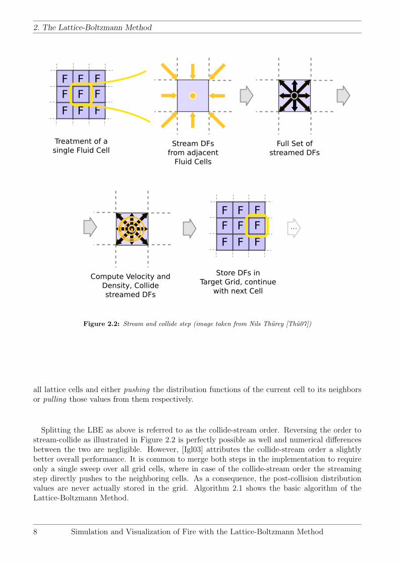
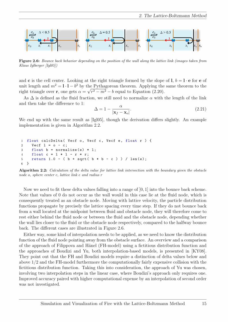
Figure 2.6: Bounce back behavior depending on the position of the wall along the lattice link (images taken fromKlaus Iglberger [Igl05])
and c is the cell center. Looking at the right triangle formed by the slope of l, b = l · e for e ofunit length and m2 = l · l− b2 by the Pythagorean theorem. Applying the same theorem to theright triangle over r, one gets α =
√r2 −m2 − b equal to Equation (2.20).
As ∆ is defined as the fluid fraction, we still need to normalize α with the length of the linkand then take the difference to 1:
∆ = 1− α
|xf − xo|. (2.21)
We end up with the same result as [Igl05], though the derivation differs slightly. An exampleimplementation is given in Algorithm 2.2.
1 float calcDelta( Vecf o, Vecf c, Vecf e, float r ) {2 Vecf l = o - c;3 float b = normalize(e) * l;4 float c = l * l - r * r;5 return 1.0 - ( b + sqrt( b * b - c ) ) / len(e);6 }
Algorithm 2.2: Calculation of the delta value for lattice link intersection with the boundary given the obstaclenode o, sphere center c, lattice link e and radius r
Now we need to fit these delta values falling into a range of ]0, 1] into the bounce back scheme.Note that values of 0 do not occur as the wall would in this case lie at the fluid node, which isconsequently treated as an obstacle node. Moving with lattice velocity, the particle distributionfunctions propagate by precisely the lattice spacing every time step. If they do not bounce backfrom a wall located at the midpoint between fluid and obstacle node, they will therefore come torest either behind the fluid node or between the fluid and the obstacle node, depending whetherthe wall lies closer to the fluid or the obstacle node respectively, compared to the halfway bounceback. The different cases are illustrated in Figure 2.6.
Either way, some kind of interpolation needs to be applied, as we need to know the distributionfunction of the fluid node pointing away from the obstacle surface. An overview and a comparisonof the approach of Filippova and Hanel (FH-model) using a fictitious distribution function andthe approaches of Boudizi and Yu, both interpolation-based models, is presented in [KY08].They point out that the FH and Boudizi models require a distinction of delta values below andabove 1/2 and the FH-model furthermore the computationally fairly expensive collision with thefictitious distribution function. Taking this into consideration, the approach of Yu was chosen,involving two interpolation steps in the linear case, where Boudizi’s approach only requires one.Improved accuracy paired with higher computational expense by an interpolation of second orderwas not investigated.
Simulation and Visualization of Fire with the Lattice-Boltzmann Method 15

2. The Lattice-Boltzmann Method
(a) Cell state modification for a moving boundary (b) Cell states after obstacle movement
Figure 2.7: Pre- and post-moving state of an obstacle (images taken from Klaus Iglberger [Igl05])
Yu’s model can be formulated as
fi(xf , t+ ∆t) =1
1 + ∆[(1−∆)fi(xf , t) + ∆fi(xo, t) + ∆fi(xf ′ , t) + 6wiρwei · uw], (2.22)
where i denotes the lattice link in direction towards, i in direction from the obstacle surface, xfis the fluid node, xo is the obstacle node associated by the lattice link, and xf ′ = xf + ei∆t.Furthermore, wi is the equilibrium distribution value, ρw is the density at the obstacle surface,and uw the obstacle velocity.
For an obstacle at rest, the last term in equation 2.22 can be skipped and the determinationof the obstacle boundary cells and computation of delta values for links intersecting the surfaceneeds only to be done once, e.g. during LBM setup phase. If the sphere is allowed to move,however, cells will need to turn from fluid cells to obstacle cells and vice versa, as shown in Figure2.7. In other words, the determination of obstacle boundary cells and delta value calculationneeds to be done for every time step, resulting in a significant additional computational effort.
16 Simulation and Visualization of Fire with the Lattice-Boltzmann Method

3 Characteristics of Fire
What actually happens when a flammable object catches fire and burns? Though this questionis far too complex to answer in detail, a short overview of the scientific aspects is necessaryto motivate a physically-based fire simulation. Nielsen and Madsen treat this matter morethoroughly in their Master’s thesis [NM99] that gives an overview of a variety of methods tomodel, animate, and visualize fire along with some physical background. Great parts of thischapter are loosely based on it.
3.1 A Physical Motivation
Contrary to popular belief, it is not the wood itself burning in a campfire, but the fuel, i.e. sapand wood oils, contained in them and driven to the surface by heat. Burning is a rapid oxidationof a flammable object caused by high temperature. Having said that, we already mentioned thethree ingredients of fire: fuel, oxygen, and heat. But what is fire? Facing this question, oneinstantaneously tends to fall back to describing its characteristics, the color, the shape, the heat,the greedy spreading, and connected dangers. We will not dare trying to answer this question,since the phenomenon of fire is far from being fully understood even by experts, but instead gothrough some general terms first, taken from [NM99].
The lowest temperature, where fuel vapor forms an ignitable mixture with air is called flashpoint. As soon as the vapor can sustain a burning flame for at least five seconds, the fire pointis reached. At the critical temperature, a flammable liquid is irrevocably turned into vapor atatmospheric pressure. Self-sustained combustion is possible above the ignition temperature,depending on a multitude of conditions such as fuel concentration, air mixture, temperature ofthe ignition source, and many more.
3.2 Categorization of Fire
Depending on external circumstances like supply of fuel and oxygen, fire develops differently andshows distinct visual characteristics. Based upon that, [NM99] try a categorization.
A calm fire is for example that of a lit candle, undisturbed by wind and resulting in an almoststatic flame. It is classified as a diffusion flame, since a sufficient amount of oxygen needs todiffuse inwards to reach the burning zone. Supply of fuel and oxygen is controlled and the flamehas no direct possibilities of spreading.
The freely fed fire permeates the whole burning object and receives virtually unlimited fueland oxygen. Vapor is advected by buoyancy forces and thus limits the flame spreading to theupward direction.
In contrast, the motion of the flammable vapor of a pressure fed fire is mainly dictatedby the fuel’s velocity vectors when leaving the pressure tank. For this kind of flame, oxygen isusually premixed with the fuel before ignition to obtain clean combustion with no soot being
17

3. Characteristics of Fire
formed. In this way, the combustion process can be controlled to a certain extent, which appliesto the temperature in particular. This type of control is for instance used in a Bunsen burnerthat can reach very high temperature regions.
A violent fire is fed somewhat more irregularly, fuel is vaporized as available. It may spreadto other flammable regions, but the spreading is mainly directed by advecting buoyancy forcesif not strongly influenced by environmental circumstances such as wind.
In this thesis, we are mainly concerned with freely or pressure fed fire, that are visually moreinteresting than a candle flame, yet fairly simple to model. The focus is put on the interactionwith external wind fields rather than the spreading of fire, which will be omitted.
3.3 The Color of Flame
In physics, light emitted solely due to an object’s high temperature is referred to as incandescence.The higher the temperature, the faster the Brownian motion of the atoms and therefore the higherthe energy the electrons gain by more frequent collisions, enabling them to rise to a higher energylevel, a quantum leap, and emitting photons when falling back to their respective base levels.This phenomenon is described as one of 15 causes of color in [Nas01].
As the object is heated, the incandescent light spectrum turns from black over red, orange,yellow and white to blue-white. The path taken in the chromaticity space of visible light depictedin Figure 3.1 is called Planckian Locus. This transition corresponds to an increase of energy ofthe light. What we perceive as “white” daylight is incandescent light emitted by the sun with asurface temperature of about 5700 �. It appears white because it is a mixture of a high numberof different wavelengths of the visible spectrum of light.
Black body radiation is a special form of incandescence. A black body is an ideal absorber thatneither reflects nor transmits any electromagnetic radiation. Specifically, no light is reflected,what makes the object appear black when cold, hence the name. But when heated, it emits acharacteristic, temperature-dependent spectrum of incandescent light, the black body radiation,displayed in Figure 3.2 for a range of 1000 to 16000K. In the resulting black body table, everypossible temperature, commonly measured in Kelvin, can be assigned a corresponding color. Theother way round, the black body palette can also be used to determine an estimate of the flametemperature given its color.
Of course this is an idealization. There is no real-world object with black body properties.Nevertheless, the color of a flame or a very hot object, imagine metalwork of a blacksmith justextracted from the forge, can give a rough temperature estimate. More specifically, one canassign a color temperature to any incandescent object by taking the temperature of a true blackbody emitter that best matches the color of the actual incandescent object.
Soot remaining from incomplete combustion, mostly carbon, is responsible for the black bodycoloring of flames. This can be demonstrated by adjusting the oxygen supply vent of a Bunsenburner. The wider open, the more oxygen reaches the combustion zone, the hotter the flame,where the color, turning from yellow-orange to blue, serves as an indicator of the temperature.In zones of residue-free combustion, as for instance in the hottest part of the flame, the flameis even translucent as no soot is present there. Real-world flame colors are moreover influencedby spectral band emission of the burning material, the characteristic emission of an elementgiven by the structure of its valence orbital. A widespread experiment in chemistry education atschools to demonstrate this phenomenon is the flame test of sodium, which gives a characteristic
18 Simulation and Visualization of Fire with the Lattice-Boltzmann Method

3. Characteristics of Fire
Figure 3.1: CIE 1931 chromaticity diagram including the Planckian locus1
4000 K1800 K 5500 K 8000 K 12.000 K 16.000 K
Figure 3.2: Black body color spectrum for 1000 - 16000K 2
Simulation and Visualization of Fire with the Lattice-Boltzmann Method 19
3. Characteristics of Fire
(low pressure)
drag
drag
convection
pressure ThermalBuoyancy
pressure
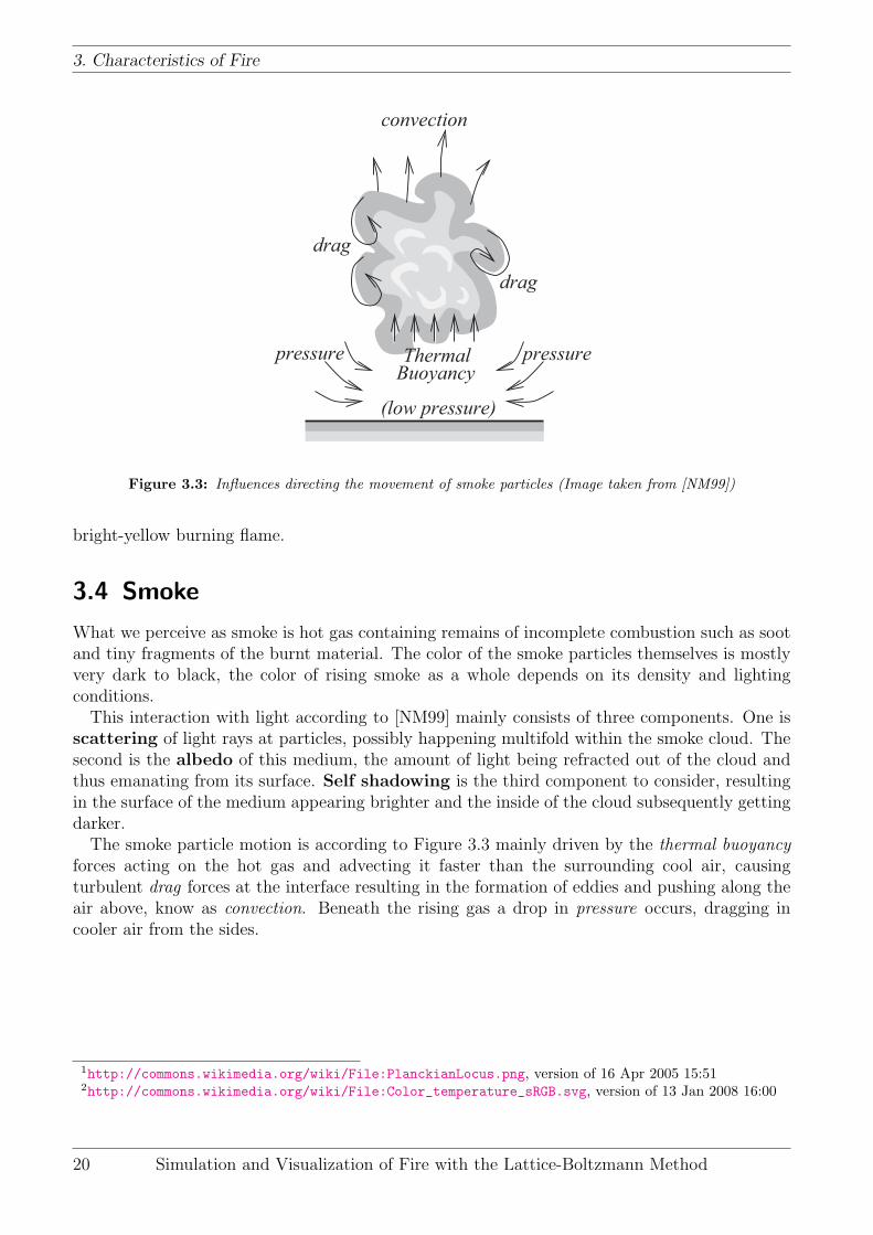
Figure 3.3: Influences directing the movement of smoke particles (Image taken from [NM99])
bright-yellow burning flame.
3.4 Smoke
What we perceive as smoke is hot gas containing remains of incomplete combustion such as sootand tiny fragments of the burnt material. The color of the smoke particles themselves is mostlyvery dark to black, the color of rising smoke as a whole depends on its density and lightingconditions.
This interaction with light according to [NM99] mainly consists of three components. One isscattering of light rays at particles, possibly happening multifold within the smoke cloud. Thesecond is the albedo of this medium, the amount of light being refracted out of the cloud andthus emanating from its surface. Self shadowing is the third component to consider, resultingin the surface of the medium appearing brighter and the inside of the cloud subsequently gettingdarker.
The smoke particle motion is according to Figure 3.3 mainly driven by the thermal buoyancyforces acting on the hot gas and advecting it faster than the surrounding cool air, causingturbulent drag forces at the interface resulting in the formation of eddies and pushing along theair above, know as convection. Beneath the rising gas a drop in pressure occurs, dragging incooler air from the sides.
1http://commons.wikimedia.org/wiki/File:PlanckianLocus.png, version of 16 Apr 2005 15:512http://commons.wikimedia.org/wiki/File:Color_temperature_sRGB.svg, version of 13 Jan 2008 16:00
20 Simulation and Visualization of Fire with the Lattice-Boltzmann Method

4 A Model of Freely Fed Fire
4.1 Overview of the Model
The implementation presented in this chapter is based on the work of Wei et al. published inthe paper “Simulating Fire with Texture Splats” [WLMK02]. They present a model of freelyfed fire that is essentially a particle system. The particles represent the individual flames andare referred to as display primitives. They are advected by a Lattice-Boltzmann computed 3Dvelocity volume representing the airflow and incorporating boundary conditions and interactionwith obstacles and environmental influences like wind fields. When inserted, each primitive isassigned a certain amount of fuel it consumes over its lifespan. As all the fuel is used up, thedisplay primitive expires and is removed from the system.
For the particle system they propose the following algorithm:
1. Inject new fire particles into the system with an initial texture and fuel value
2. Perform one step of the LBM solver to update the velocity vectors of the lattice
3. Move each fire particle according to the trilinearly interpolated velocity vector at the parti-cle’s current position. Check for particles that leave the grid or have consumed all of theirfuel and remove them from the system.
4. Compute the temperature of each particle with a linear temperature model and assign acolor to the particle according to a black body color table. If the particle temperature fallsbelow a certain threshold, convert it to a smoke particle and color it using a separate colortable. Decrease the fuel value of each particle.
5. Render the particles
4.2 Evaluation
As the authors state in [WLMK02], the presented model offers a physically-based descriptionof the evolution of fire and its interaction with the environment. It claims by no means to bephysically accurate and that is not the primary intention. The goal is computational efficiency toallow a visualization in real-time as described in the next chapter. All steps of the implementationand also the results should be regarded with this in mind.
A limitation of the model is the absence of a feedback from the temperature field back intothe LBM. In fact, this limitation is one of the LBM itself, as the D3Q19 is an isothermal modelthat cannot describe the energy transfer caused by temperature differences [WLMK04]. For adiscussion of the problems involved refer to the book of Succi [Suc01, Chapter 14], where severalthermodynamic Lattice-Boltzmann models are introduced. The author concludes that none ofthem is free from stability problems so far.
21

4. A Model of Freely Fed Fire
confparser
lbm
particles
ConfParser ConfBlock
LBM
main_lbm main_ps
Vec
boost Irrlicht
Grid
ParticleSystemParticle
Emitter
Figure 4.1: Intersection calculation of lattice link and sphere
Consequently, temperature-induced buoyancy cannot be incorporated into the LBM compu-tations. As a compromise, buoyancy forces will therefore be treated independently in the imple-mentation, while they are omitted altogether in the model of Wei et al. For the temperature-independent advecting velocity field of the LBM, however, it is necessary to explicitly prescribeinflow boundary conditions with fixed velocities as sources of the flow.
4.3 Implementation Aspects
4.3.1 Overview of the Implemented Classes
The implementation is divided into namespaces and classes as shown in Figure 4.1. As the corecomponent, the Lattice-Boltzmann fluid solver was designed completely independent of the firesimulation code. It is wrapped in the class LBM residing in the lbm namespace, can be usedwith both float and double data types, and implements all the features detailed in Chapter 2.
The namespace confparser contains the two classes ConfParser and ConfBlock responsible forparsing parameter files containing the description of the scene to simulate. These are described indetail in Section 7.1. As the parser only turns the configuration file into a format the applicationcan then query for parameter values but makes no assumption of its content, it can be used forother applications without modification.
The main component of the fire simulation is the particle system organized in the classesParticleSystem, Particle and Emitter in the namespace particles. ParticleSystem contains themain simulation loop, invoking the LBM solver and the visualization, that is separately presentedin Chapter 5. Emitter and Particle are the data structures for the particle sources and theparticles, respectively.
22 Simulation and Visualization of Fire with the Lattice-Boltzmann Method

4. A Model of Freely Fed Fire
4.3.2 Particle System Main Loop
All the components of the particle system are triggered from its main loop, defining the order ofsteps that need to be performed in every time step. We will first only concentrate on the controlof particles, omitting the visualization for the moment. As shown in Algorithm 4.1, the three coreparts are emitParticles(), where new particles enter the scene at defined inlets, calculation ofthe velocity field by calling the runStep() function of the LBM solver and updateParticles(),comprising the movement, exchange of temperature, and the check for the end of life of eachparticle.
1 setupLBM ();2 setupParticleSystem ();3
4 for ( int step = 0; step < maxSteps; ++step ) {5
6 emitParticles ();7
8 solver.runStep ();9
10 updateParticles ();11
12 }
Algorithm 4.1: Particle system main loop
4.3.3 Particles
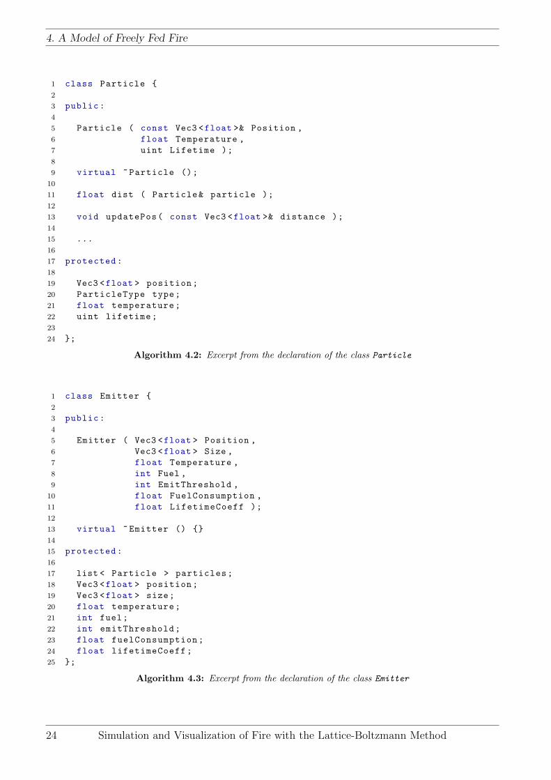
Fire is for modeling purposes abstracted by a cloud of particles characterized by the four prop-erties type, i.e. fire or smoke, position in 3D space, temperature and lifetime, a measure forthe remaining fuel. An excerpt from the class declaration is given in Algorithm 4.2. For construc-tion, the latter three properties must be specified, the type is implicitly set to fire. The functionsdist() returning the distance between the current and a given particle and updatePos() tomove the particle by a given vector will be needed in the particle update step described later.
4.3.4 Emission
New fire particles enter the scene at certain user-defined inlets constituting the sources of flame.These emitters are defined by a volume given by position and size, where new particles appearat random positions, a temperature that is set as initial temperature of newly created particles,a fuel value defining their lifespan and a list of particles emitted by this source.
The class declaration of an emitter given in Algorithm 4.3 contains three further coefficients,emitThreshold, defining the maximum amount of particles that can be emitted per time step,fuelConsumption, a factor by which the emitter’s fuel is reduced with every emission, andlifetimeCoeff, a factor defining what fraction of the emitter’s current fuel value is assignedto each particle as initial lifetime. The actual emission step is a loop over all emitters, whereeach emits a random number of particles up to its given upper threshold. Those newly createdparticles are appended to the emitter’s particle list particles and assigned a random position inthe emitter volume, initial temperature equal to the emitter temperature and lifetime according
Simulation and Visualization of Fire with the Lattice-Boltzmann Method 23
4. A Model of Freely Fed Fire
1 class Particle {2
3 public:4
5 Particle ( const Vec3 <float >& Position ,6 float Temperature ,7 uint Lifetime );8
9 virtual ~Particle ();10
11 float dist ( Particle& particle );12
13 void updatePos( const Vec3 <float >& distance );14
15 ...16
17 protected:18
19 Vec3 <float > position;20 ParticleType type;21 float temperature;22 uint lifetime;23
24 };
Algorithm 4.2: Excerpt from the declaration of the class Particle
1 class Emitter {2
3 public:4
5 Emitter ( Vec3 <float > Position ,6 Vec3 <float > Size ,7 float Temperature ,8 int Fuel ,9 int EmitThreshold ,
10 float FuelConsumption ,11 float LifetimeCoeff );12
13 virtual ~Emitter () {}14
15 protected:16
17 list < Particle > particles;18 Vec3 <float > position;19 Vec3 <float > size;20 float temperature;21 int fuel;22 int emitThreshold;23 float fuelConsumption;24 float lifetimeCoeff;25 };
Algorithm 4.3: Excerpt from the declaration of the class Emitter
24 Simulation and Visualization of Fire with the Lattice-Boltzmann Method

4. A Model of Freely Fed Fire
(xi,yj)
(xp,yp)
u(xp,yp)
up,res
v(Tp)
(xi+1,yj+1)(xi,yj+1)
(xi+1,yj)
ui,j
ui,j+1
ui+1,j+1
ui+1,j
Figure 4.2: Composition of the particle movement vector
to fuel * lifetimeCoeff. Each emission consumes part of the fuel supply that is thereforedecreased, affecting the lifespan of future particles.
4.3.5 Particle Update Step
Movement And Buoyancy
To account for the buoyancy of the hot fire and smoke particles, an additional temperature-dependent force term is introduced, directed against gravity. The governing equation is takenfrom [WLMK04] as
Fbuoyancy = Hg(Tk − Tamb), (4.1)
where g is the inverse gravity vector, H the coefficient of thermal expansion and Tamb the ambienttemperature.
The final particle movement is then given as the composition of this buoyancy force and the
Simulation and Visualization of Fire with the Lattice-Boltzmann Method 25

4. A Model of Freely Fed Fire
velocity computed by the LBM, illustrated in Figure 4.2. As the particles are not restricted tothe lattice but can reside at arbitrary positions in the domain, the LBM velocity is trilinearlyinterpolated. Care needs to be taken at the boundaries of obstacles in the domain. Where theLattice-Boltzmann computation directs the flow around the obstacle, this additional advectionterm could carry the particle inside the obstacle if not prevented by a collision detection.
Temperature Model
As the LBM is isothermal and cannot track temperature information, a simple linear heat equa-tion is employed to approximate the particle temperature over time and the heat the particlesradiate onto one another:
Tk(t) = αTk(t− 1) + β∑j 6=k
G(dkj)Tj(t− 1) (4.2)
where α is the heat conservation, β the transferability coefficient, dkj the distance between thedisplay primitives k and j, G() a Gaussian filter to approximate the effect of diffusion and Tk(0)is the predefined initial temperature.
This temperature information is needed to determine the color of a display primitive as de-scribed in Section 3.3 and decide when the fire particle turns into a smoke particle. ThereforEquation (4.2) needs to be evaluated for every particle in every time step, where the Gaussiandistribution is tabulated at distinct samples over the whole range of possible distance values.Particles lying dense within the flame’s core are effectively kept at high temperature, whereasthose towards the edge of the flame receive fewer irradiated heat and thus cool down faster.Eventually, the particle gets carried out of the core area and after cooling down below a giventhreshold, it is turned into a smoke particle.
The Algorithm
The begin of every update step is a check for particles that need to be removed from the sceneeither because they have exceeded their lifespan and used up all their fuel or because they havemoved out of the simulation domain. Next, the particles are moved by a vector composed ofthe LBM velocity at the current particle position and the buoyancy force depending on thetemperature. A collision test confirms that they will not end up in an obstacle. Otherwise, theyare only moved by the velocity coming from the LBM. Afterwards, the temperature is computedwith Equation (4.2). If it has fallen below the threshold temperature, the particle type is changedfrom fire to smoke. Finally, the particle’s lifetime is decreased. Algorithm 4.4 shows a simplifiedimplementation.
26 Simulation and Visualization of Fire with the Lattice-Boltzmann Method

4. A Model of Freely Fed Fire
1 void updateParticles () {2
3 // Go over all particles of all emitters
4 for (ParticleIterator p = particles.begin(); p != particles.end(); ++p) {5
6 // Remove particles that have left the domain , exceeded their lifetime , or
7 // cooled down to ambient temperature
8 while (outsideDomain( p->pos ) || p->lifetime == 0 || p->temp < ambTemp)9 p = particles.erase( p );
10
11 // Move particle according to fluid velocity at current position
12 Vec3 <float > v = solver.getVelocity( p->pos );13 // Buoyancy force
14 Vec3 <float > b = gravity * k * ( p->temp - ambTemp );15 // Resulting particle movement vector
16 Vec3 <float > u = b + v;17
18 // Check whether buoyancy force would carry particle into an obstacle
19 for (ObstacleIterator o = obstacles.begin(); o != obstacles.end(); ++o)20 if( o->isPointInside( p->pos + u ) ) {21 u = v;22 break;23 }24
25 // Move the particle
26 p->updatePos( u );27
28 // Update temperature
29 float tempExt = - gaussTable [0] * p->temp;30 // Add up temperature contributions of all other particles weighted by
31 // distance
32 for ( p2 = particles.begin(); p2 != particles.end(); ++p2)33 tempExt += gaussTable[ p->dist( *p2 ) ] * p2 ->temp;34 p->temp = alpha * p->temp + beta * tempExt;35
36 // If temperature has fallen below threshold , convert to smoke particle
37 if ( p->temp < smokeTemp ) p->type = SMOKE;38
39 // Decrease particle lifetime
40 p->lifetime --;41 }42 }
Algorithm 4.4: Simplified implementation of the particle update method
Simulation and Visualization of Fire with the Lattice-Boltzmann Method 27

4. A Model of Freely Fed Fire
28 Simulation and Visualization of Fire with the Lattice-Boltzmann Method

5 Visualization
In most cases, a fire simulation is targeted on producing visually pleasing and graphically richimagery, and this work is no exception in this regard. The visualization is aimed at real-timeframe rates, where the rendering is performed by the Irrlicht 3D engine. This chapter comprisesan overview of this framework, the visualization and coloring of fire and smoke particles, and aword on modeling the surroundings.
5.1 Irrlicht 3D Engine
On its official website, the author Nikolaus Gebhard describes Irrlicht as a cross-platform highperformance realtime 3D engine with a powerful high level API for creating complete 3D and2D applications like games or scientific visualization [Geb09]. Cross-platform means not onlysupport for different operating systems, but also for different rendering engines, namely OpenGL,Direct3D 8.1 and 9.0, and two different software renderers. Further criteria for choosing thisengine were the built-in support for a number of image and mesh formats, but most importantthe available library functions and that it is open source.
Irrlicht holds, as most 3D engines do, everything that needs to be drawn in the screen as scenenodes of a hierarchical scene graph. The camera is a scene node as well. Simple primitives likeboxes and spheres are readily available as objects in Irrlicht and can be pasted with a texture.More complex objects need to be loaded from a mesh file and can be placed freely in the scene.As the rendering is completely handled by the Irrlicht engine, the particle system needs to takecare of populating the scene graph with all necessary objects at the right positions and with theright properties set.
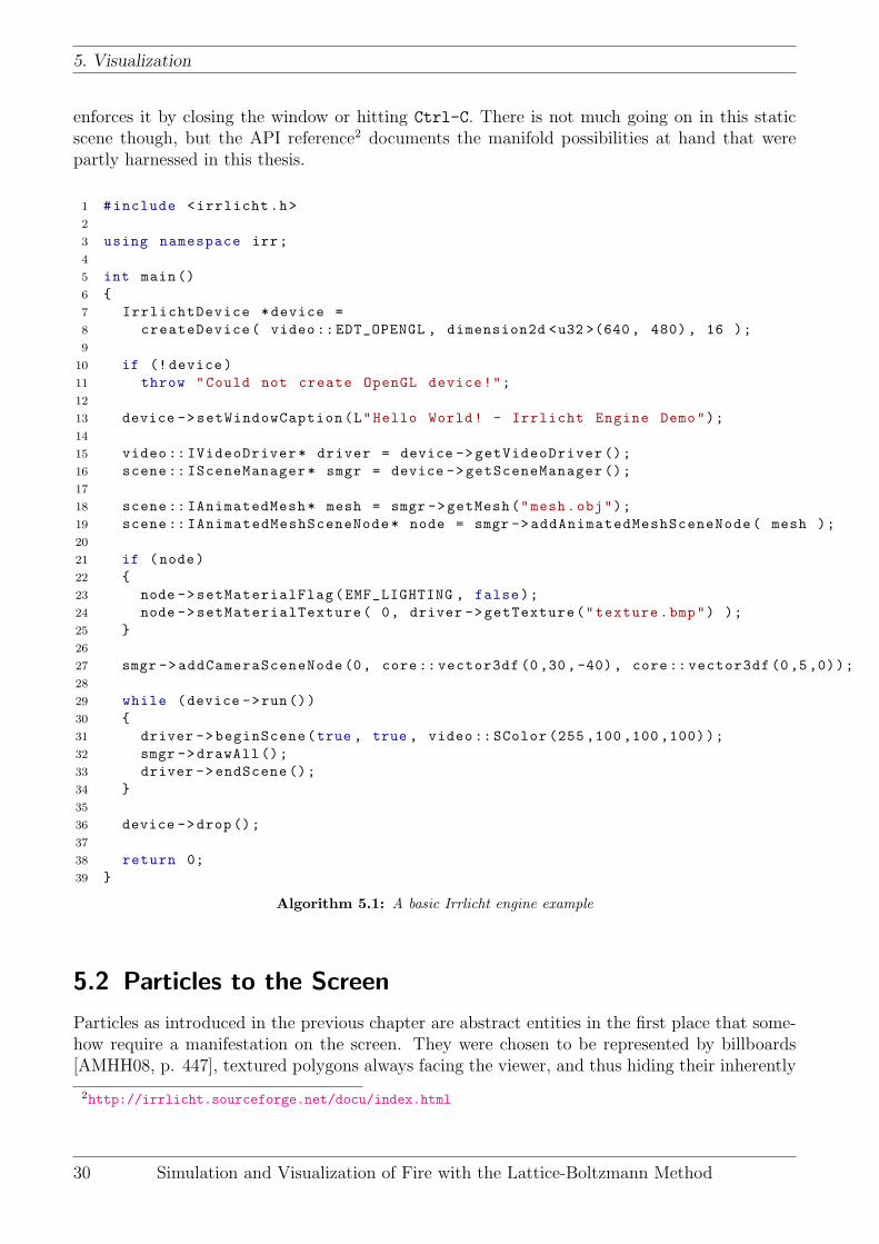
The API is quite well structured, has a steep learning curve, and a high level of abstraction,such that a working example can be developed with only a few lines of code. A demonstration isgiven by Algorithm 5.1 that is adapted from the “HelloWorld” tutorial on the Irrlicht website1.The very heart of the engine is the IrrlichtDevice, that should only be created once with thegraphics backend, desired resolution, color depth, and optionally further parameters specified.Having created that, one can access all components of the engine, most importantly the indis-pensable VideoDriver that is an interface to the system’s video driver, and the SceneManager
that provides convenient methods for populating and modifying the scene graph.
In the example, a mesh file is loaded and added to the scene after all the initialization is done.A texture is added to it and as there are no light sources in the scene, dynamic lighting is turnedoff such that the model is illuminated globally. For defining the point of view, a static camerais inserted afterwards with a fixed position and focus point. Then the main loop is started bycalling the device’s run() method. In every loop iteration, the driver is instructed to begin therendering process by calling beginScene(), then the scene manager draws everything containedin the scene graph and the video driver finishes the rendering. The loop only exits when the user
1http://irrlicht.sourceforge.net/docu/example001.html
29
5. Visualization
enforces it by closing the window or hitting Ctrl-C. There is not much going on in this staticscene though, but the API reference2 documents the manifold possibilities at hand that werepartly harnessed in this thesis.
1 #include <irrlicht.h>2
3 using namespace irr;4
5 int main()6 {7 IrrlichtDevice *device =8 createDevice( video:: EDT_OPENGL , dimension2d <u32 >(640, 480), 16 );9
10 if (! device)11 throw "Could not create OpenGL device!";12
13 device ->setWindowCaption(L"Hello World! - Irrlicht Engine Demo");14
15 video :: IVideoDriver* driver = device ->getVideoDriver ();16 scene :: ISceneManager* smgr = device ->getSceneManager ();17
18 scene :: IAnimatedMesh* mesh = smgr ->getMesh("mesh.obj");19 scene :: IAnimatedMeshSceneNode* node = smgr ->addAnimatedMeshSceneNode( mesh );20
21 if (node)22 {23 node ->setMaterialFlag(EMF_LIGHTING , false);24 node ->setMaterialTexture( 0, driver ->getTexture("texture.bmp") );25 }26
27 smgr ->addCameraSceneNode (0, core:: vector3df (0,30,-40), core:: vector3df (0,5,0));28
29 while (device ->run())30 {31 driver ->beginScene(true , true , video:: SColor (255 ,100 ,100 ,100));32 smgr ->drawAll ();33 driver ->endScene ();34 }35
36 device ->drop();37
38 return 0;39 }
Algorithm 5.1: A basic Irrlicht engine example
5.2 Particles to the Screen
Particles as introduced in the previous chapter are abstract entities in the first place that some-how require a manifestation on the screen. They were chosen to be represented by billboards[AMHH08, p. 447], textured polygons always facing the viewer, and thus hiding their inherently
2http://irrlicht.sourceforge.net/docu/index.html
30 Simulation and Visualization of Fire with the Lattice-Boltzmann Method

5. Visualization
two dimensional nature. Despite the polygon usually being a quadrilateral, they can be givenany shape by setting the texture partly transparent. Billboards are a very common choice forparticle applications, being easy to handle, very flexible in use, and at the same time cheap torender. They are very closely related to sprites [AMHH08, p. 445], images that can be movedaround freely on the screen and usually are partly transparent, as for instance the mouse cursor.But while sprites purely live in the 2D screen space and their pixels are mapped 1:1 on screenpixels, billboards do have “real” positions in the 3D scene space and are rendered together withall the other objects of the scene graph. Sprites can overlap by putting them on different layers,but this kind of depth information is completely independent of the Z-buffer based depth calcu-lations of a 3D scene. For further details, the interested reader is referred to the book “Real-timerendering” of Akenine-Moller et al. [AMHH08]. In the following, the terms sprite, billboard anddisplay primitive will be used interchangeably, though still referring to a billboard in terms ofimplementation.
As the particle update step is rather computationally expensive, a possible compromise is toperform the simulation with a smaller number of particles but add more display primitives forrendering. In other words, for each particle a predefined number of billboards is added to thescenegraph and distributed randomly in a small area around its center. Thus a visually densefire representation can also be achieved with a limited amount of particles in the simulation. Interms of implementation, the Particle class is extended by a vector of billboards and takes carethat when the particle is moved, the display primitives representing it are moved similarly.
When a billboard is added as display primitive to the scene, it is assigned a random texturefrom a pool of 32 fire textures and keeps it until its lifetime expires. The texture adds turbulentappearance to the particles. At first thought one might be tempted to change the texture at everytime step to increase the impression of turbulence, but this only creates a visual enhancement incase the texture series is continuous. Otherwise the result is just a messy-looking perturbation.
To account for the typical shape of a flame, rather round-bodied at the base and get slimmertowards the tip, the size of the billboards is adapted with the lifetime of the particle. A methodis provided to set the size of the display primitives as
size = sizebase +lifetime
lifetimeinit
· sizevar
in every time step.
5.3 Coloring
To actually resemble a flame, the cloud of particles needs to be colored appropriately. Asdescribed in Section 3.3, flame color can be approximated by that of an incandescent blackbody. To this end, a black body color table is precomputed with color samples up to double theparticles’ initial temperature in steps of 50K. During the update step, each display primitive getsassigned the tabulated color closest to its current temperature through a function provided bythe Particle class. Precisely, the billboard polygon is colored, the texture itself is a grayscaleimage and contributes the structure and transparency by acting as a weighting factor for thecolor of the underlying polygon. The same grayscale values are set again as the alpha channel.
The final flame color results from simply adding up all color values of all billboards contributingto the drawing of a particular pixel. This mode of color determination is called additive blending
Simulation and Visualization of Fire with the Lattice-Boltzmann Method 31
5. Visualization
[AMHH08, p. 139] and is given asc0 = αscs + cd (5.1)
where c0 is the resulting color value, cs is the color and αs the opacity of the current billboardreferred to as source, and cd is the resulting color of the previous step referred to as destination.
In Irrlicht this is achieved by setting the material type to EMT_TRANSPARENT_ADD_COLOR. Note,however, that the billboard texture’s grayscale value serves as αs and the polygon color as cs inthe implementation of this Irrlicht material. From a physical point of view, this makes sense,as the light reaching the viewer is superimposed from all light emitters lying in direction of thisray. Intuitively, the denser the fire, the brighter it should appear.
When a particle has turned to smoke, its color is not given by the black body palette anymore,but is set to a gray value dependent on the remaining lifespan. The color rendered to the screen isnow determined by blending the texture colors weighted by their corresponding alpha or opacityvalues with the underlying billboards from back to front, given by a formula called the overoperator [AMHH08, p. 136] defined as
c0 = αscs + (1− αs)cd (5.2)
with the same symbols as in Equation (5.1).
This differentiation is due to the fact that smoke particles do not send out light by themselves,so additive blending would lead to a wrong visual appearance. On transition from a fire to asmoke particle, the material type is changed to EMT_TRANSPARENT_ALPHA_CHANNEL to enable thisblending mode in Irrlicht. When approaching the end of their lifetime, smoke particles shouldslowly fade out instead of just vanishing from one moment to the other. An easy solution to thatwould be decreasing the overall opacity value of the billboard from time step to time step. Notsupported by any material type available in Irrlicht, this behavior is approximated by graduallydarkening the billboard polygon color so that it adapts the black background.
5.4 Environment and Lighting
As a fire burning in the pure blackness of empty space looks somewhat out of place, a fewpossibilities are provided to make the scene look more lively. First of all, an obstacle placedinto the domain, be it stationary of moving, can be set visible and pasted with a texture. It isnot necessary to provide a corresponding mesh to the object, as only spheres and axis-alignedcuboids are supported, that can be drawn using built-in functions of Irrlicht.
Secondly, any static mesh Irrlicht is capable of loading and handling can be placed at anarbitrary position into the scene, scaled if desired and a texture can be applied if the modelhas none. Irrlicht supports quite a number of file formats. Details on that can be found in thefeature list of [Geb09]. Furthermore, planes of finite extension can be placed with an arbitraryorientation into the scene and again be supplied with a texture.
Fire is most impressive in the dark, when it is the only light source available and illuminatesthe surroundings in warm color. This visual effect can be attained by dynamic lighting. Whenactivated, every billboard representing a fire particle gets a light source attached on insertion,that is deleted again as the particle turns to smoke. The color of light coming from the flamecore is modified by all the billboards it passes through on its way from the source to the surfaceit illuminates, resulting in a realistic tinge.
32 Simulation and Visualization of Fire with the Lattice-Boltzmann Method

5. Visualization
5.5 Integration into the Particle System
1 setupLBM ();2 setupParticleSystem ();3 setupIrrlicht ();4
5 for ( int step = 0; device ->run() && step < maxSteps; ++step ) {6
7 emitParticles ();8
9 driver ->beginScene ();10 sceneManager ->drawAll ();11 driver ->endScene ();12
13 solver.runStep ();14
15 updateParticles ();16
17 }
Algorithm 5.2: Visualization-enabled particle system main loop
A number of changes are required to integrate the Irrlicht-based visualization into the particlesystem. First of all, the engine needs to be initialized with the graphics backend to use and thedesired resolution similar to Algorithm 5.1. The Irrlicht main loop with the rendering of thescene graph objects is integrated into that of the particle system as demonstrated in Algorithm5.2. Population of the scene graph by the static scene environment is done during setup already,while the billboards acting as display primitives are added during the particle emission stepand are optionally equipped with light sources if dynamic lighting is enabled. They are moved,adapted in size and color, and removed again if the particle has left the domain or has consumedall its fuel.
Simulation and Visualization of Fire with the Lattice-Boltzmann Method 33

5. Visualization
34 Simulation and Visualization of Fire with the Lattice-Boltzmann Method

6 Performance Aspects
This chapter contains a discussion of the performance impact of different components of theLattice-Boltzmann fluid solver, the particle system, and the 3D visualization. All tests wereperformed on machines equipped with an Intel Core2 Duo 6400 dual core CPU, each core runningat 2.13GHz, and having 2MB L2-cache at its disposal, 2GB of main memory and an nVIDIAGeForce 7300 series video card. The code was compiled with g++ 4.2.1, linking against Irrlicht1.5.0 and Boost 1.37.0 libraries on an openSUSE Linux x86 64 operating system.
6.1 Lattice-Boltzmann Solver
The performance of Lattice-Boltzmann implementations has been measured and evaluated ingreat detail at the Chair for System Simulation, and various approaches for optimization havebeen worked out in previous theses [Don04, Igl03, Hab06]. For this thesis, however, the goal wassubstantially different. Optimization was not an important issue, so no attempts of parallelizingor blocking the LBM implementation were carried out and hence no comparison is done. Thefigures presented in the following are therefore of interest in terms of performance relations ratherthan absolute values.
6.1.1 Performance Impact of the Smagorinsky Turbulence correction
In what way the runtime and performance of the collide-stream step is influenced by activatingthe Smagorinsky turbulence correction is the first question we want to investigate. To thisend, the well-known lid-driven cavity setup, where fluid in a closed cavity is set in motion by acontinuous movement of the lid, was simulated with domain sizes of 203 up to 1203.
Figure 6.1(a) shows curves for the runtime of the collide-stream step and the full time stepincluding boundary calculations for the Smagorinsky subgrid model turned on and off. Thecurves drift apart considerably between the collision with and without the turbulence correction,whereas the boundary calculations play almost no role in terms of computation time. Measuringthe performance in millions of lattice cell updates per second (MLUP/s) reveals a significantlyhigher computational effort for the Smagorinsky-enhanced collision resulting in a performancepenalty of almost 40% (see Figure 6.1(b)). This is mostly due to the evaluation of two squareroots in the calculation of the local stress tensor, as illustrated in Equation (2.12).
6.1.2 Obstacle Boundary Conditions Compared
Another aspect worth evaluating is the computational complexity involved in obstacle boundarycalculations. As detailed in section 2.4, two different kinds were implemented: Simple cuboidshaped obstacles translating to no-slip boundaries, and spheres with curved boundaries thatcan optionally be moving. For a comparison, spheres with a radius between 5 and 50 latticeunits were placed in the center of the 1203 lid-driven cavity setup from above as obstacle in
35

6. Performance Aspects
0
200
400
600
800
1000
1200
1400
1600
20 40 60 80 100 120
Run
time
[ms]
Domain size
Smagorinsky on, completeSmagorinsky on, collide-streamSmagorinsky off, completeSmagorinsky off, collide-stream
(a) Runtime of a single LBM time step
0
0.5
1
1.5
2
2.5
20 40 60 80 100 120M
LUP
/s
Domain size
Smagorinsky off, all cellsSmagorinsky off, fluid cellsSmagorinsky on, all cellsSmagorinsky on, fluid cells
(b) Performance of the LBM implementation
Figure 6.1: LBM with and without Smagorinsky turbulence correction
(a) Staircase approximation... (b) ...blended with the correct spherical shape
Figure 6.2: Curved boundary obstacle for a sphere of radius 15
36 Simulation and Visualization of Fire with the Lattice-Boltzmann Method
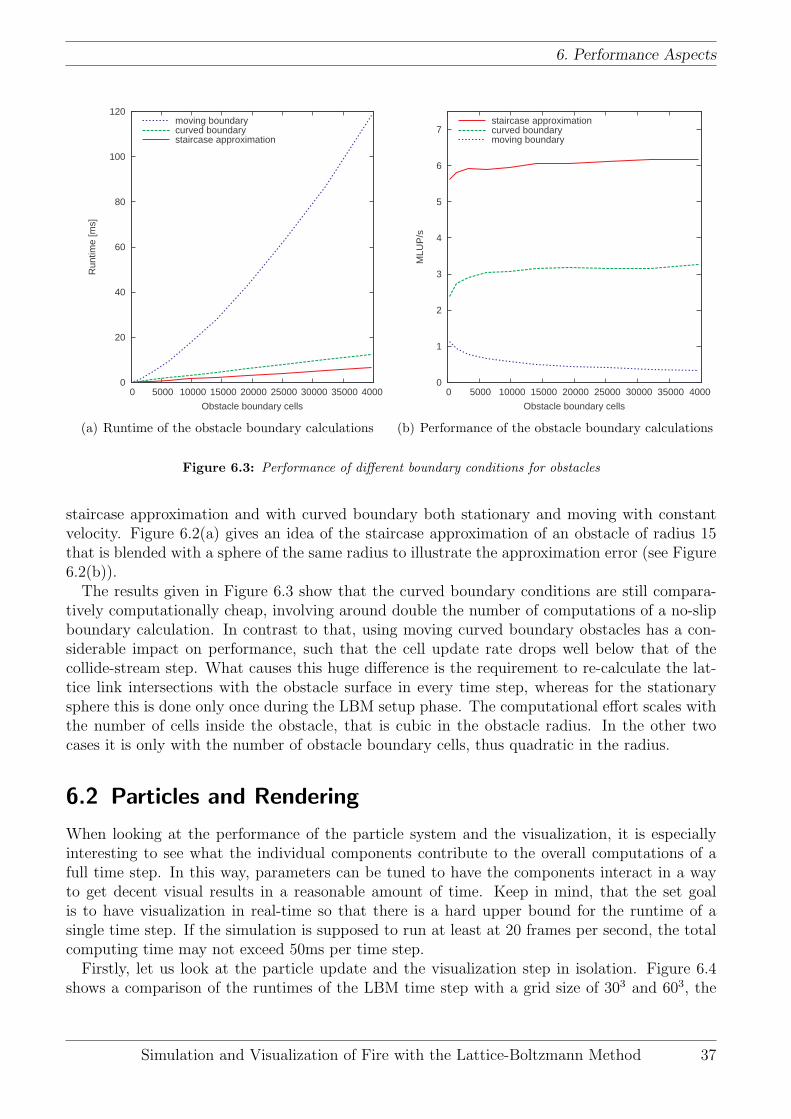
6. Performance Aspects
0
20
40
60
80
100
120
0 5000 10000 15000 20000 25000 30000 35000 40000
Run
time
[ms]
Obstacle boundary cells
staircase approximationcurved boundarymoving boundary
(a) Runtime of the obstacle boundary calculations
0
1
2
3
4
5
6
7
0 5000 10000 15000 20000 25000 30000 35000 40000
MLU
P/s
Obstacle boundary cells
staircase approximationcurved boundarymoving boundary
(b) Performance of the obstacle boundary calculations
Figure 6.3: Performance of different boundary conditions for obstacles
staircase approximation and with curved boundary both stationary and moving with constantvelocity. Figure 6.2(a) gives an idea of the staircase approximation of an obstacle of radius 15that is blended with a sphere of the same radius to illustrate the approximation error (see Figure6.2(b)).
The results given in Figure 6.3 show that the curved boundary conditions are still compara-tively computationally cheap, involving around double the number of computations of a no-slipboundary calculation. In contrast to that, using moving curved boundary obstacles has a con-siderable impact on performance, such that the cell update rate drops well below that of thecollide-stream step. What causes this huge difference is the requirement to re-calculate the lat-tice link intersections with the obstacle surface in every time step, whereas for the stationarysphere this is done only once during the LBM setup phase. The computational effort scales withthe number of cells inside the obstacle, that is cubic in the obstacle radius. In the other twocases it is only with the number of obstacle boundary cells, thus quadratic in the radius.
6.2 Particles and Rendering
When looking at the performance of the particle system and the visualization, it is especiallyinteresting to see what the individual components contribute to the overall computations of afull time step. In this way, parameters can be tuned to have the components interact in a wayto get decent visual results in a reasonable amount of time. Keep in mind, that the set goalis to have visualization in real-time so that there is a hard upper bound for the runtime of asingle time step. If the simulation is supposed to run at least at 20 frames per second, the totalcomputing time may not exceed 50ms per time step.
Firstly, let us look at the particle update and the visualization step in isolation. Figure 6.4shows a comparison of the runtimes of the LBM time step with a grid size of 303 and 603, the
Simulation and Visualization of Fire with the Lattice-Boltzmann Method 37

6. Performance Aspects
0
200
400
600
800
1000
1200
0 500 1000 1500 2000 2500 3000 3500 4000 4500 5000
Run
time
[ms]
Number of particles
LBM 303 latticeLBM 603 latticeUpdate no spritesUpdate 1 spriteRendering 1 spriteUpdate 2 spritesRendering 2 sprites
Figure 6.4: Computing time comparison of LBM, particle update and rendering
particle update step for no, one and two sprites per particle and the rendering for the lattertwo cases over the particle number. The LBM computations are completely independent of theparticle system and show the expected constant computing times. On the other hand, particleupdate and rendering are not aware of the Lattice-Boltzmann voxel grid at all and thus theirruntime is not dependent on the lattice dimensions. Instead they are directly related to thenumber of particles present in the simulation and the number of sprites representing each ofthem. The graph shows a quadratic dependence for the update time that can be explained bythe necessary temperature calculation using Equation (4.2) that has a complexity of O(n2) asevery particle interacts with each other particle. Due to the position, color, and size update forthe sprites also done in this time step, there is an additional scaling with the number of spritesper particle. As expected, the rendering time shows a linear dependence on the total number ofsprites to draw, the curves thus scale linearly with the sprites per particle.
From Figure 6.4 one can further extract how the runtimes of the individual components com-pare to each other. An LBM time step for 303 cells is outstripped by the particle update interms of computing time at a particle count of 1200, no matter if zero, one, or two sprites perparticle are rendered and plays an increasingly insignificant role for high particle counts. Thishappens with rendering time for the same particle number for one sprite, whereas for two spritesper particle the break-even is already seen for a particle number of 900. In comparison the 603
cell LBM computations are by a factor of 8 more computationally expensive, breaking even withthe “pure” particle update step at 3500, and at 3200 and 3000 particles with one and two spritesattached, respectively. The rendering times always stay below this bound for the particle countsunder consideration.
An attempt to get a better visualization of these computing time relations is made with Figures
38 Simulation and Visualization of Fire with the Lattice-Boltzmann Method

6. Performance Aspects
0
100
200
300
400
500
600
700
800
900
0 500 1000 1500 2000 2500 3000 3500 4000 4500 5000
Run
time
[ms]
Number of particles
Particle emissionRenderingLBMParticle update
(a) Runtimes summed up for one time step
0
20
40
60
80
100
0 500 1000 1500 2000 2500 3000 3500 4000 4500 5000
% o
f com
puta
tion
time
Number of particles
Particle emissionRendering
LBMParticle update
(b) Runtimes set in relation to each other
Figure 6.5: Runtimes of a full simulation time step (1 sprite per particle)
0
200
400
600
800
1000
1200
1400
0 500 1000 1500 2000 2500 3000 3500 4000 4500 5000
Run
time
[ms]
Number of particles
Particle emissionRenderingLBMParticle update
(a) Runtimes summed up for one time step
0
20
40
60
80
100
0 500 1000 1500 2000 2500 3000 3500 4000 4500 5000
% o
f com
puta
tion
time
Number of particles
Particle emissionRendering
LBMParticle update
(b) Runtimes set in relation to each other
Figure 6.6: Runtimes of a full simulation time step (2 sprites per particle)
Simulation and Visualization of Fire with the Lattice-Boltzmann Method 39

6. Performance Aspects
0
200
400
600
800
1000
1200
1400
0 500 1000 1500 2000 2500 3000 3500 4000 4500 5000
Run
time
[ms]
Number of particles
Particle emissionRenderingLBMParticle update
(a) Runtimes summed up for one time step
0
20
40
60
80
100
0 500 1000 1500 2000 2500 3000 3500 4000 4500 5000
% o
f com
puta
tion
time
Number of particles
Particle emissionRendering
LBMParticle update
(b) Runtimes set in relation to each other
Figure 6.7: Runtimes of a full simulation time step (4 sprites per particle)
0
500
1000
1500
2000
2500
0 500 1000 1500 2000 2500 3000 3500 4000 4500 5000
Run
time
[ms]
Number of particles
Particle emissionRenderingLBMParticle update
(a) Runtimes summed up for one time step
0
20
40
60
80
100
0 500 1000 1500 2000 2500 3000 3500 4000 4500 5000
% o
f com
puta
tion
time
Number of particles
Particle emissionRendering
LBMParticle update
(b) Runtimes set in relation to each other
Figure 6.8: Runtimes of a full simulation time step (8 sprites per particle)
40 Simulation and Visualization of Fire with the Lattice-Boltzmann Method

6. Performance Aspects
0
20
40
60
80
100
120
0 500 1000 1500 2000 2500 3000 3500 4000 4500 5000
Ren
derin
g tim
e [m
s]
Number of sprites
No dynamic lightingDynamic lighting (1 Object)Dynamic lighting (2 Objects)Dynamic lighting (4 Objects)Dynamic lighting (8 Objects)
Figure 6.9: Rendering time comparison for dynamic lighting turned on and off
6.5, 6.6, 6.7 and 6.8. These four pairs of graphs show the composition of the total runtime of asimulation time step and the contributions to it by the four substeps weighted in percent, oncemore plotted against the total particle count. Figures were measured for a sprite number of one,two, four, and eight per particle and the emission of particles was also taken into considerationhere. Though the latter two cases of four and eight sprites were left out in Figure 6.4 for sakeof legibility, they are given here for completeness. In terms of Lattice-Boltzmann computations,only the case of 303 cells is considered.
Not surprisingly, the graphs illustrate what was already extracted from Figure 6.4 above. TheLBM computations manifest as a constantly thick layer in the runtime graphs. While makingup for the lion’s share of computing time for low particle numbers, they very rapidly lose insignificance for high particle counts. Exactly contrary behavior can be seen from the particleupdate that clearly dominates the overall runtime for higher particle numbers. An interesting rolein between plays the rendering, steadily increasing in computational effort with an increasingnumber of sprites and having the big share somewhere in the low to center span, where thepeak is much higher for more sprites per particle. Almost of no importance when it comes tocomputing time and consequently indiscernible in the graph is the particle emission, that onlyfor the smallest particle counts has a noticeable share of overall runtime.
6.3 Dynamic Lighting
All measurements for the visualization so far have been performed with dynamic lighting dis-abled to emphasize the dependencies on particle and sprite numbers. Enabling dynamic lighting
Simulation and Visualization of Fire with the Lattice-Boltzmann Method 41
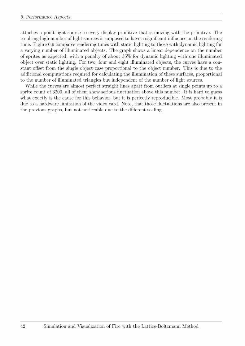
6. Performance Aspects
attaches a point light source to every display primitive that is moving with the primitive. Theresulting high number of light sources is supposed to have a significant influence on the renderingtime. Figure 6.9 compares rendering times with static lighting to those with dynamic lighting fora varying number of illuminated objects. The graph shows a linear dependence on the numberof sprites as expected, with a penalty of about 35% for dynamic lighting with one illuminatedobject over static lighting. For two, four and eight illuminated objects, the curves have a con-stant offset from the single object case proportional to the object number. This is due to theadditional computations required for calculating the illumination of these surfaces, proportionalto the number of illuminated triangles but independent of the number of light sources.
While the curves are almost perfect straight lines apart from outliers at single points up to asprite count of 3200, all of them show serious fluctuation above this number. It is hard to guesswhat exactly is the cause for this behavior, but it is perfectly reproducible. Most probably it isdue to a hardware limitation of the video card. Note, that those fluctuations are also present inthe previous graphs, but not noticeable due to the different scaling.
42 Simulation and Visualization of Fire with the Lattice-Boltzmann Method

7 Examples And Results
Visual results for selected example setups are presented in this chapter. Additionally, the neces-sary description of a scene represented by its parameter file is discussed.
7.1 The Scene Description
The simulation framework developed in the previous chapters needs to be provided with a de-scription of the scene to simulate as input. Targeting a very flexible yet powerful specificationof the required input data, a parameter file based approach was chosen. All components arehighly configurable, what gives the user maximum control of the simulation without the need tochange the implementation and recompile. In order to handle a large number of possible options,the parameter file is hierarchically organized in blocks, grouping parameters affecting the samecomponent of the simulation logically together. Where necessary, blocks can be nested to furtherincrease flexibility. This structure was inspired by the configuration files for waLBerla, the com-prehensive Lattice-Boltzmann solver developed at the Chair for System Simulation, presented in[FGD+07].
Following a well-defined syntax, the parameter file is parsed into a hierarchical tree datastructure by a custom configuration file parser. Malformed configuration files are rejected witha precise indication where the syntax error was found. The parser itself makes no distinction ofdata type of the parameters. During the individual components’ setup phases, this data structureis queried for the required configuration parameters.
A configuration file consits of the following blocks, some of them optional:
� domain (required by LBM and Particle System) Specifies the domain size in lattice cells.
� parameters (required by LBM and Particle System) Contains basic simulation parametersfor both core components, like the number of time steps to simulate.
� vtk (optional for LBM) If present, VTK output of the LBM velocity, density, and flag fieldis written to a series of files with the specified basename.
� boundaries (required by LBM) Specifies the boundary conditions. Contains the subblockstop, bottom, left, right, front, and back for the individual sides of the domain cuboidthat in turn contain subblocks for the different kinds of boundary conditions noslip,velocity, inflow, outflow, and pressure. Each of those may appear multiple times,defining a rectangular boundary patch, where the missing third coordinate is automaticallyset according to the surrounding superblock. These patches may not overlap and regionsnot covered default to no-slip.
� obstacles (optional for LBM and Particle System) May contain any number of the sub-blocks cuboid_stationary, sphere_stationary, and sphere_moving, each defining anobstacle of the given type by size, location, and for the last kind velocity.
43

7. Examples And Results
(a) 1000 particles, 1000 sprites (b) 800 particles, 1600 sprites
(c) 500 particles, 2000 sprites (d) 300 particles, 2400 sprites
Figure 7.1: Simulation after 100 time steps for different numbers of sprites displayed
� particles (required by Particle System) Holds the parameters specific to the particlesystem and the subblocks defining the emitters. The emitter parameters are specifiedaccording to Section 4.3.4.
� irrlicht (optional) If present, the Irrlicht OpenGL visualization is enabled with the spec-ified parameters. This block also contains subblocks defining the fire textures and optionalstatic meshes or planes to be inserted into the scene.
7.2 Example Setups and Visual Results
In this section, results of simulation runs are presented in form of screenshots.
7.2.1 Influence of Varying Sprite Number per Particle
To begin, we want to pick up the thought from Section 6.2 on the maximum number of spritesthat are possible in order to still sustain an interactive 20 frames per second. For this timeconstraint of 50ms per time step, a maximum particle number of 1000, 800, 500, and 300 wasmeasured on the test system for 1, 2, 4, and 8 sprites per particle. A visual comparison of acampfire with the resulting total sprite counts of 1000, 1600, 2000, and 2400 can be seen inFigure 7.1. Obviously the fire appears slightly more dense from (a) to (d). In cases where this isintended, increasing the number of sprites per particle results in a performance benefit. There
44 Simulation and Visualization of Fire with the Lattice-Boltzmann Method

7. Examples And Results
Figure 7.2: A soccer ball shot through a campfire with and without dynamic lighting
is a caveat however, in that the temperature calculations are solely based on the particles, thusvarying their number affects the temperature distribution and leads to different results.
7.2.2 Dynamic Lighting
A far more obvious visual difference makes the activation and deactivation of dynamic lighting.Figure 7.2 shows a scene, where a soccer ball is shot through a campfire. Dynamic lighting createsa very different visual quality, colors appear bright where those of the constantly lit scene seemrather dull in comparison. The result looks much more realistic and convincing so that for theremaining scenes to show, it will always be enabled.
7.2.3 Selected Example Scenes
To convey an impression what kinds of simulations are possible with the framework, a selectionof example scenes is presented in this subsection.
The first one is a campfire blown over by a strong wind from one side (see Figure 7.3). Aninflow boundary patch in the otherwise no-slip bottom of the domain creates the advecting flowfor the emission source, one of the sides is set to inflow to model the wind and the remainder isan outflow region, where the flow can leave the domain. The wood and stones of the campfireare inserted as a static mesh that does not interact with the flow. Furthermore, a plane pastedwith a grass texture represents the ground.
An extension of the scenario used in Section 7.2.2 to demonstrate the effect of dynamic lightingcan be seen in Figures 7.4 and 7.5: Instead of a single soccer ball, two and three soccer ballsare shot through the fire, respectively. They are shot in from different corners such that theypass through the fire one after another. As the screenshots show, the balls suppress the airwhen crossing the fire, or rather the particles in the simulation, and drag them behind a little,leaving a small particle gap afterwards. The fire is advected by the same inflow as in the previousexample, but this time all but the bottom plane is set to outflow.
A teapot placed on the campfire as example of a resting obstacle can be seen in Figure 7.6.The teapot itself is a static mesh just like the logs and stones of the campfire and cannot interactwith the flow. Therefore the shape of the teapot was approximated by a spherical obstacle of
Simulation and Visualization of Fire with the Lattice-Boltzmann Method 45
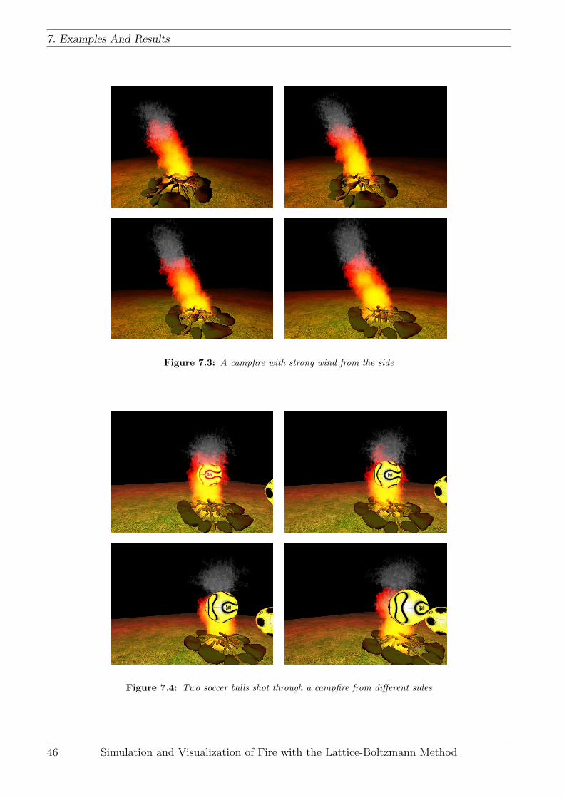
7. Examples And Results
Figure 7.3: A campfire with strong wind from the side
Figure 7.4: Two soccer balls shot through a campfire from different sides
46 Simulation and Visualization of Fire with the Lattice-Boltzmann Method
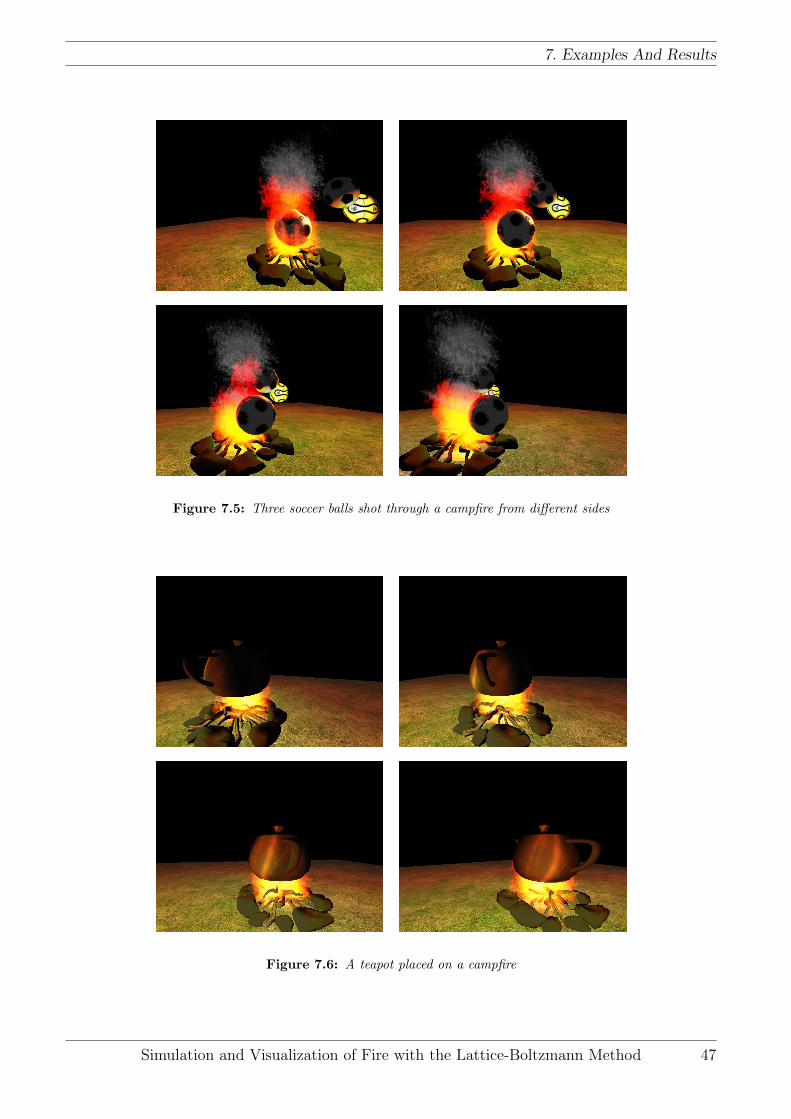
7. Examples And Results
Figure 7.5: Three soccer balls shot through a campfire from different sides
Figure 7.6: A teapot placed on a campfire
Simulation and Visualization of Fire with the Lattice-Boltzmann Method 47

7. Examples And Results
Figure 7.7: A teapot placed on a stove inside a room
Figure 7.8: A fire calmly burning in a fireplace
appropriate radius. Inflow and outflow were defined the same way as in the two previous setups.The flames obviously spread a lot broader here, as they are blocked in their natural upwardmotion. However, they seem not to be able to pass by the teapot and ascend.
The same teapot placed on a stove in a small room is depicted in Figure 7.7. In this scenariosmoke can only exit through a chimney below the ceiling. The teapot is modeled the same wayas in the previous scene and similarly the flames are kept below the pot and cannot pass by thesides. Figure 7.8 shows another indoor scene, a fire calmly burning in a fireplace, where againthe airflow is channeled by the chimney, that is the only way out. There is a bit of convectioninto the room though, recognizable by the smoke particles in the right image. In both scenariosthe whole domain boundary is a fixed wall, apart from an inlet patch on the floor and an outletin the ceiling, where the chimney ends. The brickwork of stove and chimney in Figure 7.7 is alsomodelled as no-slip boundary, just like the coving of the fireplace that is not visible in Figure7.8.
7.2.4 Evaluation of the Results
The presented screenshots demonstrate that the visualization is capable of creating a convincingdepiction of fire based on the data coming from the particle system and the underlying LBM. Allthis is far from being photo-realistic, but is delivered in real-time and with interactive frame rates,while it is possible to freely navigate through the scene. The soccer ball scenarios demonstratethe interaction with the environment in a physically sound way, whereas the teapot scenariosexhibit limitations of the underlying model.
48 Simulation and Visualization of Fire with the Lattice-Boltzmann Method

8 Conclusion
Simulation of freely fed fire advected by a Lattice-Boltzmann calculated flow field was successfullydemonstrated in this thesis. To this end, an LBM fluid solver was developed and extended bya Smagorinsky subgrid model to cope with turbulent flows, and the handling of various kindsof boundary conditions, including moving curved boundaries of obstacles. As core componentof the fire simulation, a particle system based on the model of Wei et al. [WLMK02] wasimplemented. It features a linear temperature model, can handle fire as well as smoke, and wasextended by provision for buoyancy forces that are combined with the LBM-computed velocityfield to determine the particle movements. Integration of the Irrlicht 3D engine adds visualizationin real-time, where textured billboards are used to represent the particles on the screen. Theircoloring is performed according to the current temperature using a black body color table lookup.Furthermore, a file parser was developed to extract parameters from configuration files containinga scene description in a way they can be retrieved in the setup phase of the simulation.
The LBM proves to be an apt tool for handling environmental influences like wind fieldsand obstacles in the flow, delivering high performance while keeping the implementation fairlysimple. Sufficiently accurate results can already be achieved on rather coarse grids. Harnessingthe possibilities of the versatile configuration approach, complex scenarios for simulation can bedescribed easily. The presented performance results demonstrate that the set goal of interactiveframe rates can be reached on modern hardware even for complex scenarios, as the visualizationallows the number of displayed particles to be kept quite low without losing much detail. Thusit is possible to move around in the scene in real-time while the simulation is running.
There still remain many open points to work on, however. As the implementation was notexplicitly targeted on performance, there is a high potential for optimization left. The LBMsolver could be extended for instance by parallelization, blocking, and grid compression tech-niques. Adaptive coarsening or grid refinement could also prove worth investigating in order tosimulate the critical regions around obstacle boundaries in more detail while saving clock cyclesin areas of homogeneous flow. A very promising way to go lies in porting the Lattice-Boltzmanncomputations to the GPU using a GPGPU framework such as CUDA. Impressive results har-nessing state-of-the-art GPU compute power for the LBM have been given in [Hab08, Tol08].Looking at the particle system, the quadratic complexity of the temperature calculations is aweak point. Limiting the heat exchange only to particles nearby by introducing a cutoff radiusor space partitioning could bring this problem to a linear complexity class.
Apart from performance optimization, a number of functional extension are conceivable. Ontop of the list is the possibility for the flames to spread, which requires tracking the fire front asZhao et al. have done in [ZWF+03]. The catching on fire of flammable objects could be easilyintegrated in such a model as well. For modeling more realistic scenes, insertion of arbitrarypolygonal meshes as obstacles, possibly even moving, into the voxel lattice would be a nice-to-have feature, especially in combination with spreading of fire fronts. A point so far not solvedsatisfactory according to [Suc01, Chapter 14] is a coupling of the temperature model back intothe LBM. It could nevertheless be worth evaluating current thermal LBM model to see whetheror not they provide an alternative.
49
8. Conclusion
For the visualization part, volume rendering techniques like blobs or textured splats as demon-strated in [WLMK02] could be employed to increase visual quality. Staying with the chosenapproach, a sound way for alternating the textures of the display primitives could create visuallymore pleasing results, as could a proper fading of the smoke particles. Incorporating furthervisual effects like heat-based refraction blurring objects seen through the fire or a more realisticillumination are also conceivable.
Finally, the parameterization could be made more intuitive by allowing real-world quantitiesto be specified instead of the somewhat abstract lattice quantities where appropriate. Thehigh number of parameters required could be alleviated by providing more default values andcombining given parameters to determine the values of others where possible. More interactionand fine-grained control of the simulation could be attained by providing the user with aninterface to change certain parameters at runtime with immediate effect.
50 Simulation and Visualization of Fire with the Lattice-Boltzmann Method

Bibliography
[AMHH08] T. Akenine-Moller, E. Haines, and N. Hoffman. Real-Time Rendering 3rd Edition.A. K. Peters, Ltd., Natick, MA, USA, 2008.
[Don04] S. Donath. On Optimized Implementations of the Lattice Boltzmann Method onContemporary Architectures. Bachelor’s Thesis, Aug 2004. Betr. Wellein, Hager,Zeiser, F. Deserno.
[FGD+07] C. Feichtinger, J. Gotz, S. Donath, K. Iglberger, and U. Rude. Concepts of waLBerlaPrototype 0.1. Technical Report 07-10, 2007.
[Geb09] N. Gebhardt. Irrlicht engine - a free open source 3d engine. website, April 2009.
[Hab06] J. Habich. Improving computational efficiency of Lattice Boltzmann methods oncomplex geometries. Bachelor’s Thesis, Dec 2006. Betr. Hager, Wellein, Zeiser(RRZE), U. Rude.
[Hab08] J. Habich. Performance Evaluation of Numeric Compute Kernels on NVIDIA GPUs.Master’s thesis, IMMD10, Jul 2008.
[HSCD96] S. Hou, J. Sterling, S. Chen, and G. D. Doolen. A lattice boltzmann subgrid modelfor high reynolds number flows. Fields Institute Communications, 6:151–166, Jan1996.
[Igl03] K. Iglberger. Performance Analysis and Optimization of the Lattice BoltzmannMethod in 3D. Studienarbeit, Sep 2003. Tutor M. Kowarschik.
[Igl05] K. Iglberger. Lattice-Boltzmann Simulation of Flow around moving Particles. Mas-ter’s thesis, Jun 2005. Betr. N. Thurey.
[KCR00] S. A. King, R. A. Crawfis, and W. Reid. Fast volume rendering and animation ofamorphous phenomena. In In Proc. International Workshop on Volume Graphics,pages 229–242, 2000.
[KY08] P. H. Kao and R. J. Yang. An investigation into curved and moving boundarytreatments in the lattice Boltzmann method. Journal of Computational Physics,227(11):5671–5690, 2008.
[Nas01] K. Nassau. The Physics and Chemistry of Color: The Fifteen Causes of Color, 2ndEdition. Wiley, July 2001.
[NM99] T. E. Nielsen and S. T. Madsen. Modelling, animation, and visualization of fire.Master’s thesis, University of Copenhagen, Denmark, April 1999.
51

Bibliography
[Per85] K. Perlin. An image synthesizer. In B. A. Barsky, editor, Computer Graphics(SIGGRAPH ’85 Proceedings), volume 19, pages 287–296, July 1985.
[PH89] K. Perlin and E. M. Hoffert. Hypertexture. In Jeffrey Lane, editor, ComputerGraphics (SIGGRAPH ’89 Proceedings), volume 23, pages 253–262, July 1989.
[QdL92] Y. H. Qian, D. d’Humieres, and P. Lallemand. Lattice BGK model for Navier-Stokesequation. Europhysics letters(Print), 17(6):479–484, 1992.
[Ree83] W. T. Reeves. Particle systems – a technique for modeling a class of fuzzy objects.ACM Trans. Graphics, 2:91–108, April 1983.
[Suc01] S. Succi. The Lattice Boltzmann Equation for Fluid Dynamics and Beyond. OxfordUniversity Press, Oxford, 2001.
[Thu07] N. Thurey. Physically based Animation of Free Surface Flows with the Lattice Boltz-mann Method. PhD thesis, FAU Erlangen, 2007.
[Tol08] J. Tolke. Implementation of a Lattice Boltzmann kernel using the Compute UnifiedDevice Architecture developed by nVIDIA. Computing and Visualization in Science,pages 1–11, 2008.
[WG00] D. A. Wolf-Gladrow. Lattice-Gas, Cellular Automata and Lattice Boltzmann Models,An Introduction. Lecture Notes in Mathematics. Springer, Heidelberg, Berlin, 2000.
[WLMK02] X. Wei, W. Li, K. Mueller, and A. Kaufman. Simulating fire with texture splats. InIEEE Visualization, pages 227–234, 2002.
[WLMK04] X. Wei, W. Li, K. Mueller, and A. Kaufman. The lattice-boltzmann method forsimulating gaseous phenomena. IEEE Transactions on Visualization and ComputerGraphics, 10(2):164–176, 2004.
[WZF+03] X. Wei, Y. Zhao, Z. Fan, W. Li, S. Yoakum-Stover, and A. Kaufman. Blowing in thewind. In SCA ’03: Proceedings of the 2003 ACM SIGGRAPH/Eurographics sympo-sium on Computer animation, pages 75–85, Aire-la-Ville, Switzerland, Switzerland,2003. Eurographics Association.
[ZWF+03] Y. Zhao, X. Wei, Z. Fan, A. Kaufman, and H. Qin. Voxels on fire. In VIS ’03:Proceedings of the 14th IEEE Visualization 2003 (VIS’03), page 36, Washington,DC, USA, 2003. IEEE Computer Society.
52 Simulation and Visualization of Fire with the Lattice-Boltzmann Method