Embed Size (px)
Citation preview

Examensarbete vid Institutionen foumlr geovetenskaper ISSN 1650-6553 Nr 264
A climatological study of Clear Air Turbulence over the North Atlantic
A climatological study of Clear Air Turbulence over the North Atlantic
Leon Lee
Leon Lee
Clear Air Turbulence (CAT) is the turbulence experienced at high altitude on board an aircraft The main mechanisms for its generation are often said to be Kelvin-Helmholtz instability and mountain waves CAT is an issue to the aviation industry in the sense that it is hard to predict its magnitude and exact location Mostly it is just a nuisance for the crew and passengers but occasionally it causes serious injuries and aircraft damage It also prevents air-to-air refuelling to be conducted in a safe manner The micro scale nature of CAT makes it necessary to describe it with turbulence indices
The first part of this study presents a verification of the two commonly used turbulence indices TI1 and TI2 developed by Ellrod and Knapp in 1992 The verification is done with AMDAR (Aircraft Meteorological Data Relay) reports and computed indices from ERA-Interim data The second part presents a 33-year climatology of the indices for describing CAT Results show that the index TI1 is generally the better of the two indices based on hit rate but TI2 performs better based on false alarm rate The climatology suggests that CAT is more frequent at the northern east coast of the US over the island of Newfoundland and east of Greenland In the vertical CAT seems to occur most frequently at the 225 hPa level but also occur frequently at the 300 hPa level at the aforementioned areas Based on AMDAR reports from 2011 only 0014 of the reports were positive turbulence observations The low amount of reports suggests that CAT can be avoided effectively with current CAT predicting skills and flight planning
Uppsala universitet Institutionen foumlr geovetenskaperExamensarbete E1 Meteorologi 30 hpISSN 1650-6553 Nr 264Tryckt hos Institutionen foumlr geovetenskaper Geotryckeriet Uppsala universitet Uppsala 2013
Examensarbete vid Institutionen foumlr geovetenskaper ISSN 1650-6553 Nr 264
A climatological study of Clear Air Turbulence over the North Atlantic
Leon Lee
Copyright copy Leon Lee och Institutionen foumlr geovetenskaper Luft‐ vatten‐ och landskapslaumlra
Uppsala universitet
Tryckt hos Institutionen foumlr geovetenskaper Geotryckeriet Uppsala universitet Uppsala 2013
3
Abstract
A climatological study of Clear Air Turbulence over the
North Atlantic
Leon Lee
Clear Air Turbulence (CAT) is the turbulence experienced at high altitude on board an
aircraft The main mechanisms for its generation are often said to be Kelvin-Helmholtz
instability and mountain waves CAT is an issue to the aviation industry in the sense that it
is hard to predict its magnitude and exact location Mostly it is just a nuisance for the crew
and passengers but occasionally it causes serious injuries and aircraft damage It also
prevents air-to-air refuelling to be conducted in a safe manner The micro scale nature of
CAT makes it necessary to describe it with turbulence indices
The first part of this study presents a verification of the two commonly used turbulence
indices TI1 and TI2 developed by Ellrod and Knapp in 1992 The verification is done
with AMDAR (Aircraft Meteorological Data Relay) reports and computed indices from
ERA-Interim data The second part presents a 33-year climatology of the indices for
describing CAT Results show that the index TI1 is generally the better of the two indices
based on hit rate but TI2 performs better based on false alarm rate The climatology
suggests that CAT is more frequent at the northern east coast of the US over the island
of Newfoundland and east of Greenland In the vertical CAT seems to occur most
frequently at the 225 hPa level but also occur frequently at the 300 hPa level at the
aforementioned areas Based on AMDAR reports from 2011 only 0014 of the reports
were positive turbulence observations The low amount of reports suggests that CAT can
be avoided effectively with current CAT predicting skills and flight planning
Keywords CAT clear air turbulence turbulence indices climatology North Atlantic
ERA-Interim AMDAR
Department of Earth Sciences Uppsala University Villavaumlgen 16 SE-752 36 Uppsala
4
Referat
En klimatologisk studie av Clear Air Turbulence oumlver
Nordatlanten
Leon Lee
Clear Air Turbulence (CAT) aumlr den turbulens paring houmlg houmljd som upplevs ombord paring flygplan
och orsaken till denna turbulens saumlgs ofta vara Kelvin-Helmholtz-instabilitet och laumlvaringgor
Paring grund av svaringrigheten att foumlrutsaumlga dess styrka och exakta position aumlr CAT ett problem
inom flygbranschen Ofta aumlr CAT bara ett irritationsmoment foumlr besaumlttning och
passagerare men kan ibland orsaka personskador och flygplansskador Den mikroskaliga
strukturen som CAT har goumlr det noumldvaumlndigt att beskriva den med turbulensindex
Den foumlrsta delen av denna studie tar upp paringlitligheten av tvaring ofta anvaumlnda turbulensindex
TI1 och TI2 utvecklade av Ellrod och Knapp aringr 1992 Verifikationen goumlrs med hjaumllp av
AMDAR-rapporter (Aircraft Meteorological Data Relay) och turbulensindex beraumlknade
med data fraringn ERA-Interim Den andra delen bestaringr av en 33-aringrs klimatologisk studie av
CAT baserat paring dessa index Baserat paring traumlffgrad presterar TI1 generellt baumlttre aumln TI2 men
TI2 presterar baumlttre aumln TI1 vad gaumlller falsklarmsgrad Den klimatologiska studien tyder paring
att CAT aumlr mer frekvent oumlver USAs norra ostkust oumlver Newfoundland och oumlster om
Groumlnland I vertikalled verkar CAT foumlrekomma mest frekvent omkring 225 hPa-nivaringn
men aumlven runt 300 hPa-nivaringn oumlver de geografiska omraringden som naumlmnts ovan AMDAR-
rapporter fraringn 2011 visar att endast 0014 av rapporterna observerade turbulens Den
laringga andelen antyder att man effektivt kan undvika CAT oumlver nordatlanten med branschens
nuvarande foumlrmaringga att foumlrutse CAT och god faumlrdplanering
Nyckelord CAT clear air turbulence klarluftsturbulens turbulensindex klimatologi
nordatlanten ERA-Interim AMDAR
Institutionen foumlr geovetenskaper Uppsala universitet Villavaumlgen 16 752 36 Uppsala
5
Table of Contents
1 Introduction 7
11 Background 7
12 Objectives 7
2 Theory 8
21 Theory of turbulence 8
22 Description of Clear Air Turbulence 9
23 Causes of Clear Air Turbulence 9
231 Kelvin-Helmholtz instability 9
232 Gravity Waves 11
24 Turbulence indices 12
25 The indices TI1 TI2 and DTI 12
26 ERA-Interim 16
27 Aircraft Meteorological Data Relay and Turbulence Reporting 17
3 Methodology and Data 20
31 Obtained ERA-Interim data 20
32 Computing TI1 and TI2 20
33 Obtained AMDAR data 22
34 Verification with AMDAR reports from 2011 23
35 Climatological study over the North Atlantic Ocean 24
4 Results 26
41 Performance of TI1 26
42 Performance of TI2 26
43 Geographical frequency plots 27
431 North Atlantic overview 27
432 Vertical distribution along the 655degN and 30degW cross section 27
44 Vertical distribution of CAT with AMDAR reports from 2011 28
5 Discussion 32
51 The use of TI1 and TI2 as CAT indicator 32
52 CAT climatology of the North Atlantic 33
6 Conclusions 35
7 Acknowledgements 36
References 37
Appendix A Frequency plots of TI1
Appendix B Frequency plots of TI2
6
7
1 Introduction
11 Background
Clear Air Turbulence (CAT) is a phenomenon associated with inflight bumpiness on board an aircraft flying at high altitude Mostly it is just a nuisance requiring passengers to remain seated with their seat-belts fastened but occasionally the turbulence can be of such high magnitude resulting in aircraft damage (Clark et al 2000) and serious injuries (Sharman et al 2012) Due to the micro scale nature of CAT it is a difficult problem in predicting its occurrence and location Several different definitions of CAT exist but most authors agree that CAT is non-convective turbulence generated by either Kelvin-Helmholtz instability or by mountain waves
Over the last decades several turbulence indices have been developed to predict CAT among others the commonly used TI1 and TI2 indices (Ellrod and Knox 2010) based on the horizontal deformation and the local instantaneous convergence The horizontal deformation and the local instantaneous convergence can be linked to frontogenesis and increased vertical wind shear being a triggering mechanism for Kelvin-Helmholtz instability (Ellrod and Knapp 1992) The TI1 and TI2 indices are in operational use at several national aviation forecast offices worldwide (Overeem 2002 Bergman 2001 Turp and Gill 2008) The TI1 was also used in a climatological study by Jaeger and Sprenger (2007)
This study is part of the EU funded project REsearch on a CRuiser Enabled Air Transport Environment (RECREATE) with the ultimate goal to show that on a preliminary design level cruiser-feeder operations can comply with airworthiness requirements for civil aircrafts It has been shown that a cruiser-feeder concept can reduce fuel consumption and its associated CO2 emissions by 23 (Maringrtensson et al 2011) For a cruiser-feeder system concept two aircrafts need mid-air contact to exchange fuel (ie air-to-air refuelling) or payload CAT is a hazard to such operations and can make them impossible to be performed in a safe way
This study evaluates the performance of the TI1 and TI2 indices with AMDAR (Aircraft Meteorological Data Relay) reports and studies the CAT climate over the North Atlantic with the aforementioned indices using a 33-year data set from ERA-Interim the most recent global atmospheric reanalysis stretching over the period from 1979 and onwards
12 Objectives
This study will try to answer
1 Based on AMDAR reports how reliable are the turbulence indices TI1 and TI2 for describing CAT
2 How does the CAT climatology over the North Atlantic look like based on the indices computed with 33 years of data from ERA-Interim
8
2 Theory
21 Theory of turbulence
In fluid mechanics any fluidic flow can either be laminar or turbulent The laminar flow is a
smooth flow that is easily predictable On the other hand turbulence is characterised by its
irregularity since it is a non-linear system that acts in all directions The detailed evolution
of a turbulent flow can be predicted by using Direct Numerical Simulation (DNS) to solve
the Navier-Stokes equations However the computational cost of DNS is extremely high
even for the most powerful computers to date Turbulence can thus not be predicted easily
Turbulence is diffusive and mixes fluid properties and affects different scales Stull (1988)
describes turbulence as irregular swirls of different sizes Due to the dissipative nature
bigger swirls turn into smaller swirls and eventually dissipate into heat ndash this is called the
cascade effect One way to statistically describe turbulence in the atmosphere is to quantify
it by averaging the wind into a mean part and a perturbation part The turbulence can then
be regarded as the perturbation that is deviating from the mean wind
Atmospheric turbulence can be divided into two categories Although the two types of
turbulence share the same properties when fully developed they can be induced by
different mechanisms One of them is the mechanically induced turbulence which is
created when there is wind shear The wind shear can be created either by surface friction
for example a rough landscape or by larger higher-rising obstacles Strong wind shear can
also be found in the upper troposphere near the jet streams where the wind velocity can
differ considerably within a short distance The other type of turbulence is thermally
induced normally due to unequal surface heating creating convection Locally warmer air
parcels will rise causing the surrounding air to become turbulent One way to determine if
a flow is turbulent in the atmosphere is by studying the Richardson number in equation
(21)
( ) (21)
Where
is the buoyancy
is the vertical potential temperature gradient and
is the
vertical wind shear One can consider the potential temperature gradient as the thermal part
and the vertical wind shear the mechanical part A fluidic flow becomes turbulent when Ri
decreases below a certain value commonly 025 Thus we can see that when the
atmosphere is unstable and prone to convection the thermal part of the equation becomes
negative resulting the Ri to be negative also If the mechanical part is large ie the wind
shear is strong Ri will also be small We can therefore conclude that turbulence will occur
9
in an atmosphere that is unstable andor has a strong wind shear Note also that turbulence
will be inhibited by a stable atmosphere if the wind shear is not strong enough
22 Description of Clear Air Turbulence
In the aviation industry the expression Clear Air Turbulence (CAT) is used to describe
phenomena related to the turbulence that is experienced on board an aircraft The term is
actually misleading when used in aviation due to the fact that airplane shaking could as well
be induced by wave-like phenomena that is not characterised as turbulence in the fluid
dynamical sense Reiter (1964) therefore calls it ldquobumpiness-in-flightrdquo instead because that
is really what we can directly associate CAT with when mentioned in in-flight observations
It is also hard to quantify since for a given meteorological condition different aircraft
models can experience different magnitudes of CAT due to aircraft-specific parameters as
for example mass wingspan and cruising speed
In literature there are several different definitions of CAT ranging from the simple
ldquoturbulence experienced outside cloudsrdquo to the more elaborate ldquoa generic term in that it
represents turbulence occurring in statically stable shear layers which need not be cloud-
free but may contain non-convective cloudsrdquo More examples of definition of CAT can be
found in a report by Overeem (2002) Although there are many different definitions of
what CAT is most of them have in common that CAT describes something non-
convective in high altitude Some authors include mountain waves in the definition some
do not In this report mountain waves are chosen to be included in the definition as they
also can give ldquobumpiness-in-flightrdquo However the indices used later in this report do not
take into account mountain waves or convection that can produce CAT
The typical CAT areas are approximately 80-500 km in the wind direction and 20-100 km
perpendicular to it Vertically they can stretch 500-1000 m (Overeem 2002 citing Met
Office College) Most CAT encounters are reported in baroclinic zones with a stable
stratificated lapse rate The onset of CAT causes mixing within the turbulent layer which
results in an adiabatic layer between two inversions Statistical studies have shown that 71
of all reported CAT encounters occurred in the vicinity of a jet stream (Reiter 1964)
Encounters are also more frequent over mountains and continents than over flat terrain
and oceans
23 Causes of Clear Air Turbulence
231 Kelvin-Helmholtz instability
Kelvin-Helmholtz instability (KHI) is generally seen as the main mechanism of CAT
formation (Ellrod and Knapp 1992) The phenomenon occurs when there is a sufficiently
large vertical wind shear within a stable layer and produces breaking waves that lead to
CAT although a large static stability can inhibit KHI development if the wind shear is not
strong enough These conditions are often present close to the jet stream Due to its
10
dependence on the vertical wind shear and the atmospheric stability the Richardson
number (equation (21)) would be a suitable parameter to describe the onset of KHI
Howard and Miles (1964) suggested that KHI often occurs when Ri is close to 025
however there is a poor correlation between Ri and CAT (Ellrod and Knapp 1992 citing
Dutton 1980)
KHI can be reproduced in the lab by letting two fluid of different density move in the
opposite direction in a laminar fashion When the shear is large enough the small turbulent
motion in the shearing zone between the two fluids will grow and initiate a wave form with
the characteristic KH waves This occurs when the following condition in equation (22) is
true
( ) (
) (22)
Figure 21 Evolution of Kelvin-Helmholtz instability between two fluids in a direct numerical
simulation Colours show density in the transition layer (Smyth and Moum 2012)
copy The Oceanography Society Reprinted with permission
Where and are the velocity and density of the respective fluids denoted by their indices
is the acceleration of gravity and is the wave number From the equation we can see
that the right side becomes larger with a stronger difference in density Thus in order for
KHI to develop the shear on the left hand side needs to be larger in such case Applied on
11
the atmosphere this means that with a stronger stratification a larger wind shear is required
for KHI to develop
Due to the instability these waves eventually break down leaving a turbulent layer with a
reduced stability and shear Figure 21 shows the typical evolution of KHI between two
fluids In the atmosphere this process can sometimes be seen with the naked eye if there
are clouds present in the shearing layer as the clouds will be reformed to the characteristic
billow cloud-form see figure 22
Figure 22 Kelvin-Helmholtz clouds seen at Uppsala 2012-03-24 (Photo Leon Lee)
232 Gravity Waves
Although some authors do not consider mountain waves as a source of CAT there have
been several cases where severe CAT was encountered in areas with no significant KHI-
favourable conditions One example is an event at 1305 UTC on the 25th of May 2010
where a Boeing 777-200B encountered severe CAT over western Greenland A 5-km
numerical simulation produced large-amplitude lee waves in good agreement with the event
coordinates (Sharman et al 2012) The meteorological conditions consisted of a low
pressure centred south of the top of Greenland producing an easterly flow at all altitudes
The Ri was large at all levels due to a relatively weak wind shear suggesting an absence of
KHI The scorer parameter given in equation (23) is a parameter originating from the wave
equation and is often used to describe flow over a mountain range
(23)
Where radic
is the Brunt-Vaumlisaumllauml frequency of which when squared is the same as
the nominator in the Richardson number equation (21) When the scorer parameter is
constant with height conditions are favourable for propagating mountain waves If the
scorer parameter decreases with height conditions are favourable for trapped lee waves As
for the event on 25th May 2010 the scorer parameter decreased sharply at the occurred
12
CAT level (Sharman et al 2012) A case study by Reiter and Nania (1964) concerning CAT
and jet stream structure found a steady decrease of the scorer parameter at the studied area
suggesting that lee wave parameters are valuable as CAT forecasting aids in the vicinity of
mountain ranges On two other occasions of severe CAT at high altitudes the scorer
parameter was observed to be fairly constant with height at the reported CAT altitudes
while the Ri was large at most heights (Lee 2011)
24 Turbulence indices
Several indices exist to predict CAT the TI1 which takes into account horizontal
deformation and vertical wind shear the TI2 which is similar to TI1 but includes a
convergence term the Brown index taking into account the horizontal deformation and
absolute vorticity and the Dutton index which is originating from a multiple linear
regression analysis with a comprehensive pilot survey based on horizontal and vertical wind
shear Overeem (2002) used numerical model data and computed the mentioned indices
and also the vertical wind shear the horizontal wind shear and the frontogenesis alone to
verify their validity with PIREP (Pilot Reports) and AMDAR (see section 27) reports The
results of that study showed that TI2 performed the best although most of the indices
overestimated the CAT areas giving significant false-alarm ratios This is probably due to
the micro scale nature of CAT In a 44-year climatological study of CAT indices over the
Northern Hemisphere (Jaeger and Springer 2007) the TI1 Ri Brunt-Vaumlisaumllauml frequency and
negative potential vorticity were used
There is also a statistical approach where several of the mentioned and other indices are
used together and weighted in relation to their importance (Sharman et al 2006) the
Graphical Turbulence Guidance-2 (GTG2) It performed well and gave good probability of
detection rate Still the TI indices are in operational use at aviation forecasting offices in
several countries (Ellrod and Knox 2010) for example at the Dutch KNMI (Royal
Netherlands Meteorological Institute) (Overeem 2002) the TI1 is used at the Swedish
SMHI (Swedish Meteorological and Hydrological Institute) (Bergman 2001) the TI2 is used
and Met Office in the United Kingdom have implemented the indices as well (Turp and
Gill 2008) The indices are popular due to their performance computational speed and easy
implementation In a further improvement of TI1 a divergence trend term is added to
account for rapid divergence changes associated with anticyclonic shear and gravity wave
generation in cyclonic regions (Ellrod and Knox 2010) It should be noted that most of the
indices discussed in literature do not take into account turbulence associated with mountain
waves
25 The indices TI1 TI2 and DTI
One of the components of the TI indices developed by Ellrod and Knapp (1992) is the
horizontal deformation (DEF see equation (24)) which is the arithmetic length of the
deformation caused by stretching (DSH see equation (25)) and the deformation caused by
horizontal shearing (DST see equation (26))
13
radic (24)
(25)
(26)
Figure 23 illustrates how horizontal wind shear DSH can give an increase in the potential
temperature gradient The horizontal stretching can also give a tightening of the isotherms
but this requires the angle (β) between the isotherms and the axis of dilatation to be smaller
than 45deg This is illustrated in figure 24 The deformation is a property that elongates a
circular-area shaped fluid to an elliptical shape Higher deformation gives larger elongation
Figure 23 Tightening of isotherms by horizontal wind shear Solid lines are isotherms and
arrows illustrate the wind shear
Figure 24 Tightening of isotherms by horizontal stretching Arrows are streamlines and solid
lines are isotherms β is the angle between the isotherms and the axis of dilatation (red line)
14
In the case of TI2 a convergence term is included (CVG see equation (27)) When
streamlines of air confluences or when the air decelerates as in the case at the exit region
of a jet streak convergence occurs Since we assume the air in the atmosphere to be
incompressible an area of convergence will give rising or sinking air at these regions
Convergence in the upper troposphere results in descending air and may create gravity
waves in the tropopause region which could trigger KHI (Ellrod and Knapp 1992)
(
) (27)
The TI1 and TI2 indices are derived by starting with Petterssens (1956) equation of
frontogenetic intensity seen in equation (28)
( ( ) ) (28)
Where is the frontogenetic intensity is the potential temperature gradient and is
the angle from the axis of dilatation to the potential temperature isotherms (see figure 24)
The equation is approximated for a constant pressure surface where is the
frontogenetic intensity on that surface The potential temperature gradient is approximated
by the sensible temperature gradient with n being the perpendicular axis to the isotherms
(Ellrod and Knapp 1992 Mancuso and Endlich 1966) see equation 29
(29)
This means that the factor between potential temperature and sensible temperature is
approximated to be 1 but according to the equation (210) of potential temperature for air
at the pressure levels between 500 and 150 the factor can vary between 12 and 17
Overeem (2002) also points out that the temperature approximation is doubtful
(
)
(210)
The aforementioned approximations then yield equation (211)
( ( ) ) (211)
15
The thermal wind relationship given in equation (212)
(212)
where = Coriolis parameter = acceleration of gravity and
= vertical wind shear =
VWS can then substituted into equation (211) Ellrod and Knapp also approximate the
cosine term to be 1 maximizing the deformation term This yields equation (213)
( ) (213)
The above equation suggests that frontogenesis will give an increased vertical wind shear
which would then suggest an increased risk of CAT occurrence Mancuso and Endlich
(1966) found that the product of vertical wind shear and deformation gave the best
correlation with CAT generation 043-048 Thus Ellrod and Knapp (1992) simplified
(213) and defined the turbulence index TI1 to be as equation (214)
(214)
Ellrod and Knapp also defined a second turbulence index which takes into account the
convergence term seen in equation (215)
( ) (215)
TI1 has been used in operational aviation forecasting in several countries and is popular
due to its good performance simple definition and computing cost-friendly nature (Ellrod
and Knox 2010) In a verification study with pilot surveys and AMDAR Overeem (2002)
found that the two indices give best performance among other indices They do however
overestimate the CAT areas although Overeem points out that the indices are still useful
TI1 and TI2 are based on the hypothesis that frontogenesis would create stronger thermal
gradients that in turn would lead to an increased vertical wind shear triggering KHI In an
effort to improve the TI1 Ellrod and Knox (2010) added a divergence trend term DVT
(equation (216)) to the index The combination of deformation and changes in divergence
is said to capture both frontogenesis and spontaneous gravity wave generation in cyclonic
flows while in anticyclonic flows the divergence trend term also will function as a CAT
indicator
16
((
)
(
)
) (216)
The subscripts h1 and h2 represent different forecast intervals where the divergence trend
is to be calculated The divergence trend term is simply added to TI1 to give to new
divergence-modified turbulence index DTI seen in equation (217)
(217)
Ellrod and Knox (2010) assigned C in equation (216) the value of 01 in order to make the
DVT of the same magnitude In their verification they found DTI to perform better than
TI1 in strong anticyclonic shear andor curvature and also in cyclonic flows in the exit
region of strong jets The DTI also performed better spatially compared to TI1 in the
mentioned regions However for other meteorological conditions the DTI and TI1 only
had minor differences due to the fact that the DVT was not of significant size
26 ERA-Interim
A global atmospheric reanalysis is a dataset created by atmospheric numerical models
using observations from ground weather stations satellites atmospheric soundings aircraft
meteorological reports etc These data are fed as input into the reanalysis model and are
assimilated to produce an atmospheric state giving several meteorological parameters at the
modelled heights and grid points at a given time This is desirable due to the fact that the
observed data is not distributed evenly over the globe and not measured at the same time
As for the North Atlantic the coverage of data is usually small compared to the available
data over the continents Reanalysis datasets are therefore essentially interpolations of the
available data They are useful in climate research as they typically span over several
decades
At the time of writing ERA-Interim is the latest global atmospheric reanalysis produced by
the European Centre for Medium-Range Weather Forecasts (ECMWF) Its data is
produced with a December 2006 version of the ECMWF Integrated Forecast Model used
for operational forecasting between December 2006 and June 2007 (version Cy31r2) It
currently covers the period from 1 January 1979 and onwards with 6-hourly gridded
estimates of three-dimensional meteorological variables A previous released reanalysis
from ECMWF the ERA40 covers the period mid-1957 to 2001 The ERA-Interim
contains improvements from ERA40 and is a preparation for a future release of a next-
generation reanalysis project that will span the whole twentieth century replacing the
ERA40 (Dee et al 2011) It operates with an atmospheric-ocean-wave coupled model with
60 levels in the vertical with the top level at 01 hPa Its Gaussian grid system comprises of
a north-south grid spacing of about 0703125deg The east-west separation varies with latitude
but is also about 0703125deg at the tropics
17
The number of observations used in ERA-Interim is approximately 106 to 107 per day
depending on decade All of these observations are subject to a number of different quality
controls and data selection steps Examples of such control and selection are check for
completeness of reports physical coherence hydrostatic consistency etc Data that fail any
of these checks are flagged for exclusion A few types of observational data are spatially
dense both globally and locally for example data from satellites or wind profilers These
types of data are thinned to a proper level for the analysis method
The upper-air wind observations of ERA-Interim come from several sources From remote
sensing atmospheric motion data are provided by geostationary satellites Wind data is also
obtained from wind profilers in North America Europe and Japan Actual in situ
observations are done by atmospheric soundings pilot balloons dropsondes and aircraft
reports Despite the availability of several data sources wind information remains limited in
large parts of the atmosphere The globally averaged Root Mean Square (RMS) error in
upper-air winds from short-range forecasts produced in ERA-Interim was around 38-57
ms at June 1979 This can be compared with ERA40 which had a RMS error of 40-64
ms at June 1979 The background wind error estimates of the operational ECMWF for
June 2007 was 35-45 ms
Full resolution data from ERA-Interim can be retrieved in either GRIB or NetCDF format
from the ECMWF data server (Berrisford et al 2011) Many parameters can be retrieved
but for this study the upper-air parameters are the most relevant These parameters are
available on 60 model levels and 37 pressure levels with a time resolution of 6 hours at 00
06 12 and 18 UTC More information about the retrieved data used for this study can be
found in section 31
27 Aircraft Meteorological Data Relay (AMDAR) and Turbulence Reporting
Aircraft Meteorological Data Relay (AMDAR) is a worldwide operational automatic
reporting system A comprehensive description of the AMDAR observing system can be
found in the reference manual published by the World Meteorological Organization
(WMO 2003) This section will give a general description of AMDAR and its turbulence
reporting systems
Most of the commercial aircrafts are equipped with sensors providing meteorological and
navigational data that are sophistically processed in real-time This data serves as input to
several systems on board for example flight management and navigational systems The
data is also fed into the flight data recorder (commonly known as the ldquoblack boxrdquo) to aid
special investigations in case of incidents or accidents The meteorological parameters are
automatically sent to ground stations via satellite or radio links every 7-10 minutes and are
then relayed to National Meteorological and Hydrological Services As at November 2012
there are 38 participating airlines worldwide producing over 300 000 observations per day
18
with information on air temperature wind speed and wind direction on the observed
location
Turbulence is not directly measured on-board the aircrafts Instead the vertical acceleration
is used as a proxy parameter for quantifying turbulence This is one of the reasons to why
we should treat CAT as ldquobumpiness-in-flightrdquo (as discussed in Section 22) because
aircrafts do not necessarily have to experience turbulence in the meteorological sense when
experiencing vertical accelerations The turbulence reported in AMDAR is thus not an
objective measurement as it is aircraft-specific depending on the mass of the aircraft
altitude and airspeed For each AMDAR observation the peak value of the vertical
acceleration since the last observation is used to report turbulence It can be reported in
three ways
Variation in vertical acceleration
The peak acceleration is used to classify the severity of the turbulence according to table
21 This type of turbulence reporting is used in the obtained AMDAR data described in
section 33
Table 21 Turbulence categories in AMDAR observations
Peak Acceleration
Deviation (-+) Turbulence Category Reported value in AMDAR
Less than 015g None 0
015g to but not including
05g
Light 1
05g to 10g Moderate 2
Greater than 10g Severe 3
Derived Equivalent Vertical Gust
The Derived Equivalent Vertical Gust (DEVG) is an alternative indicator that takes into
account aircraft-specific variables and the air speed It is defined as the instantaneous
vertical gust velocity which superimposed on a steady horizontal wind would produce the
measured acceleration of the aircraft The DEVG is given in equation (218)
(218)
Where is the DEVG A is a parameter that depends on the aircraft type mass altitude
and the Mach number is the total mass of the aircraft is the modulus of the peak
19
acceleration deviation from 10g and is the calibrated airspeed at the time of the
acceleration peak occurrence
The DEVG can be compared between different aircraft types due to its aircraft
independent characteristics However the DEVG seems not to have been correctly
implemented over the Northern Hemisphere as the reported values are either
instantaneous values or peak values over 21 minutes hence not very useful for turbulence
studies (Overeem 2002)
Eddy Dissipation Rate
The Eddy Dissipation Rate (EDR) describes the vertical gust spectrum of the turbulent air
around the aircraft with the parameter by relating the vertical acceleration of the
aircraft with a response function It is given in equation (219) A more detailed derivation
of the EDR can be found in the AMDAR manual (WMO 2003)
( ) ( )
int ( )
(219)
Where is the EDR is the measurement interval is the output vertical
acceleration power is the true airspeed is the vertical acceleration response function
of the aircraft and the integral represents the vertical gust energy spectrum The integral
limits and are turbulent frequencies relative to the aircraft chosen to filter out
frequencies of no interest To simplify on board calculation the integral is pre-calculated in
look-up tables
Comparisons have been made between EDR and DEVG and show high correlation
between peak EDR and peak DEVG (WMO 2003) More simulations and reviews are
needed to verify that EDR is aircraft-independent hence it is still not in operational use
(Overeem 2002)
20
3 Methodology and Data
31 Obtained ERA-Interim data
The ERA-Interim data obtained for this study ranges from 1 January 1979 until 31
December 2011 Values of the u- and v-component of the wind and the geopotential
height at 11 pressure levels (150 175 200 225 250 300 350 400 450 500 550 hPa) were
used to compute the turbulence indices The time resolution was 6-hourly with data values
at 00 06 16 and 18 UTC The area of interest was defined as 30deg N to 705deg N and
8025deg W to 30deg E covering the North Atlantic see figure 31 The grid space distance was
075deg in both the latitudinal and the longitudinal direction This means that our domain
consists of 148 grid points along a given latitude and 55 grid points along a given longitude
Figure 31 The spatial domain of the obtained ERA-Interim data spans most of the North Atlantic
The longitudinal grid spacing of 075deg corresponds to a distance of about 83 km at all
latitudes and the latitudinal spacing of 075deg corresponds to a distance of about 72 km at
30deg N and about 28 km at 705deg N
32 Computing TI1 and TI2
The horizontal partial derivatives of the wind components found in the DEF and CVG
terms needed for TI1 and TI2 are approximated with a central finite difference method In
other words in order to calculate
(see equation (31)) on a two-dimensional grid point B
(xy) we need values from each side of that point since we want the point to be in the
centre The values used for the calculation would therefore be the points A (x-1y) and C
(x+1y) illustrated in figure 32
21
Figure 32 Values from point A and C are used to approximate the partial derivatives at
point B
Equation (31) describes the approximation of
at point B
(31)
Where is the distance between two grid points In our case the distance varies as the grid
spacing in x-direction becomes smaller when moving further north In the calculations the
distance between two longitudes separated with 1deg at the equator is assumed to be
111319492 m A more general approximation for
could then be described by equation
(32)
( )
( )
( ) ( ) ( )
(32)
Similarly the terms in the y-direction are calculated in the same fashion with the distance
between two latitudes separated with 1deg assumed to be 111132944 m
The vertical wind shear between two pressure levels is approximated by equation (33)
radic( )
( )
radic( )
( )
( ) (33)
Where the (xyz) is the value from the top of the layer and (xyz-1) is the value at the
bottom of the layer The height between the levels is calculated by dividing the difference
in geopotential height with the acceleration of gravity Note that the vertical wind
shear is calculated for a layer between two pressure levels and not a discreet pressure level
When computing TI1 and TI2 the DEF and CVG used are the averaged value of the DEF
and CVG at the bottom and the top of the layer The indices are computed at all grid
22
points (except the points at the boundaries) and between all pressure levels resulting in 10
layers with 146 and 53 equally spaced grid points in x-direction and y-direction respectively
33 Obtained AMDAR data
The used AMDAR observations in this study are within the region 40N to 70N and 60W
to 10W The data comprises of reports for the whole year of 2011 and were obtained from
the UK Met Office According to Met Office around 30 000 AMDAR reports are
received per day on average but only 500-600 contain entries for turbulence reporting
Only observations with a turbulence report were obtained for the study where a reported
turbulence degree value of 0 also is considered a valid turbulence report Observations
from 2011-01-31 and 2011-03-31 are missing
Figure 33 AMDAR reports with non-turbulence reports as blue dots and light turbulence reports as red stars
A total of 226 159 reports were obtained where nearly all of the observations are of
turbulence degree 0 ie no turbulence (see table 21) Only 32 observations reported light
turbulence (value 1) It is to be emphasized that currently most of the transatlantic flights
are heavy jet aircrafts with around 250-400 passenger seats or even more The large mass
would require stronger turbulence to experience an equivalent vertical acceleration
deviation than for smaller jets This means that for a given meteorological condition light
turbulence experienced by a large jet could be experienced as moderate or even severe
turbulence for smaller jets Figure 33 shows the geographical locations of the AMDAR
observations
23
34 Verification with AMDAR reports from 2011
Each AMDAR observation is matched to a calculated value of TI1 and TI2 at the
approximately same position and time Assuming an aircraft cruises at a ground speed of
500 knots the covered distance during 7 minutes (time between each AMDAR report) is
roughly 110 km With our grid resolution that would cover at least two grid cells or more
depending on latitude As mentioned in section 27 each turbulence report uses the
measured peak value during this time period Thus the exact location of the encountered
turbulence is not known For simplicity we match the location of reporting to the
corresponding grid cell The largest value of TI1 and TI2 at the four corners are then
matched to the observation see figure 34
Figure 34 The largest value of TI1 and TI2 among the grid points A B C and D is matched to
the AMDAR observation
To match a turbulence report to the specific pressure layer corresponding to its height the
Barometric formula in equation (34) is used to estimate the atmospheric pressure when
assuming standard atmospheric conditions This is actually a correct estimation because the
reported altitude in AMDAR reports is a pressure altitude calculated from atmospheric
pressure readings assuming the International Standard Atmosphere defined by the
International Civil Aviation Organizations (ICAO) in 1964 (WMO 2003)
(
)
(34)
Where is the local atmospheric pressure and is the reported observation height For the
International Standard Atmosphere the other parameters are constants defined as in table
31
24
Table 32 Parameters defined in the International Standard Atmosphere
Variable Value
00065 Km Tropospheric lapse rate
28815 K Temperature at sea level
980665 ms2 Acceleration of gravity
00289644 kgmol Molar mass of dry air
831447 Jmol K Universal gas constant
For example if an AMDAR report was reported at an atmospheric pressure of 252 hPa it
will be matched with the grid values from the layer 250-300 hPa
Only reports that are within 2 hours from a time step are used for the verification For
example reports between 22 and 02 UTC are coupled to the corresponding 00 UTC TI
values from ERA Interim Observations reported at 21 UTC will be excluded since they are
neither close enough to the 18 UTC time step nor the 00 UTC time step
The probability of turbulence detection is computed for chosen TI thresholds of 210-7 s-1
and 1210-7 s-1 These thresholds are based on Ellrod and Knapp (1992) and are also used
on another climatological study by Jaeger and Sprenger (2007) The results are presented in
a contingency table illustrated in table 32 Note that the amount of turbulence reports is
far less than the non-turbulence reports
If an AMDAR reports turbulence (reported value gt 0) then it is categorized as ldquoAMDAR
Yesrdquo while if it reports no turbulence (reported value = 0) then it is categorized as
ldquoAMDAR Nordquo TI values that are equal to or larger than the threshold values are
considered as positive indication of turbulence ldquoTI Yesrdquo Values below the threshold are
categorized as ldquoTI Nordquo
Table 32 Contingency table
TI Yes TI No Total
Hits Misses Tot AMDAR Yes
False alarms Correct negatives Tot AMDAR No
Total Total TI Yes Total TI No
35 Climatological study over the North Atlantic Ocean
Based on the thresholds of 210-7 s-1 and 1210-7 s-1 (Ellrod and Knapp 1992 Jaeger and
Sprenger 2007) a frequency study is done on all grid points and all pressure layers both in
the whole period of 1979-2011 but also seasonal periods with winter classified as
25
December January February (DJF) spring as March April May (MAM) summer as June
July August (JJA) and autumn as September October November (SON) By plotting the
results on a geographical map turbulence maxima are located The results will also be
plotted along one chosen latitude and one chosen longitude showing the frequency
distribution in the vertical
The obtained AMDAR reports will also be used to give further information of the CAT
distribution along the vertical
26
4 Results
41 Performance of TI1
Table 41-2 shows the performance of TI1 with the thresholds of 210-7 s-1 and 1210-7 s-1
With the lower threshold TI1 hits 96 of all the turbulence reports but has a false alarm
of 64 The higher threshold reduces the false alarm to 7 but misses 70
Table 41 Probability of detection with AMDAR using TI1 gt= 210-7 s-1
TI1 Yes TI1 No Total
22 (96) 1 (4) 23
102080 (64) 56886 (36) 158966
Total 102102 56887
Table 42 Probability of detection with AMDAR using TI1 gt= 1210-7 s-1
TI1 Yes TI1 No Total
7 (30) 16 (70) 23
10887 (7) 148079 (93) 158966
Total 10894 148095
42 Performance of TI2
Table 43-4 shows the performance of TI2 with the thresholds of 210-7 s-1 and 1210-7 s-1
The lower threshold gives 74 hits lower than for TI1 The false alarm rate is similar to
TI1 The higher threshold misses 70 of the reports same percentage as for TI1 but has a
false alarm of 13 slightly higher than TI1
Table 43 Probability of detection with AMDAR using TI2 gt= 210-7 s-1
TI2 Yes TI2 No Total
17 (74) 6 (26) 23
100793 (63) 58173 (37) 158966
Total 100810 58179
Table 44 Probability of detection with AMDAR using TI2 gt= 1210-7 s-1
TI2 Yes TI2 No Total
7 (30) 16 (70) 23
20257 (13) 138709 (87) 158966
Total 20264 138725
27
43 Geographical frequency plots
431 North Atlantic overview
Figure 42 shows the relative frequency of TI1 and TI2 values above 210-7 s-1 in all pressure
levels during the winter and the summer season with blue colour indicating low frequent
areas and red colour high frequent areas Both indices have maxima in the winter seasons
with red areas around Newfoundland and the Denmark Strait The Newfoundland location
is in agreement with a similar study of the TI1 index done by Jaeger and Sprenger (2007)
but high frequencies at the area around the Denmark Strait is not seen in that study
The notable difference between the two indices is that during the winter season TI2 has its
maximum east of Newfoundland while TI1 has its maximum in the areas east of Greenland
Differences can also be seen in figure 43 which is similar to figure 42 but with values
above 1210-7 s-1 (note the different colour scales) In general during winter TI1
concentrates its largest values over the east coast of Greenland above 68degN with a
frequency of around 6 TI2 mostly has its largest values along the east coast water of
Greenland with a frequency of around 11 The indices show little difference in the
location of maxima during the summer seasons with the high frequent area being at 56-
64degN and 20-40degW for both indices It is to be emphasized that the TI2 frequencies are
generally higher than for TI1
Frequency plots of the autumn and spring seasons for TI1 and TI2 can be found in
Appendix A and Appendix B respectively
432 Vertical distribution along the 655degN and 30degW cross section
Figure 41 Illustration of the cross sections at latitude 645degN and longitude 30degW
Figure 44 shows the relative frequency of TI1 gt 210-7 s-1 along the cross section at the
latitude of 645degN (left in the figure) and at the longitude of 30degW (right in the figure) The
cross sections are illustrated in figure 41
28
During the summer season (lower figures) the highest frequencies (~65) occur around
225 hPa on latitudes north of 56degN at all longitudes of our domain Between the latitudes
of 47degN and 56degN the high frequent area seem to increase its height southwards reaching
maximum at the 175-200 hPa South of this area frequencies generally fall below 20
During the winter seasons (top figures of 44) high frequency areas (~60) reaches further
down to as low as the lowest pressure levels of 500-550 hPa at some locations Along the
latitude cross section this can be seen around the longitude of 40degW where the east coast
of Greenland is situated Between longitudes 13degW and 40degW that is between the east
coast of Greenland and the east of Iceland the highest frequencies occur at 300 hPa Along
the longitude cross section high frequency areas generally reach further down the more
north the latitudes are
44 Vertical distribution of CAT with AMDAR reports from 2011
Of the 226159 AMDAR reports described in section 33 only 32 reported light turbulence
That is 0014 of all reports No reports reported moderate or severe turbulence Among
the 32 positive turbulence reports 12 occurred at 250-300 hPa Further up in altitude at
the pressure layer 200-250 hPa 9 positive observations were reported However at this
layer the amount of non-turbulence report was 130677 so the percentage of positive
turbulence at this particular layer is only 0007 This can be compared with the layer 250-
300 hPa (mentioned earlier) where the percentage of turbulence reports at that layer were
001 The highest positive turbulence percentage per layer was found to be in the layer
150-200 hPa with 10 reports corresponding to 004 of all reports at that layer Table 45
shows the vertical distribution of the AMDAR reports
Table 45 Vertical distribution of obtained AMDAR reports
Light turbulence count ( in layer) Non-turbulence count
150-200 hPa 10 (004) 23520
200-250 hPa 9 (0007) 130677
250-300 hPa 12 (001) 70740
300-350 hPa 1 (008) 1181
250-400 hPa 0 6
400-450 hPa 0 1
450-500 hPa 0 1
500-550 hPa 0 0
gt 550 hPa 0 1
TOTAL 32 226127
29
Figure 42 Left column - frequency of TI1 values above the threshold value of 210-7 s-1 Right column - frequency of TI2 values above the threshold value of 210-7 s-1 Top images depict the winter season and bottom images depict the summer season The colour scale is the same for all images
TI1 gt 210-7
s-1
TI2 gt 210-7
s-1
30
Figure 43 Left column - frequency of TI1 values above the threshold value of 1210-7 s-1 Right column - frequency of TI2 values above the
threshold value of 1210-7 s-1 Top images depict the winter season and bottom images depict the summer season Note the different colour scales on the left and the right side
TI1 gt 1210-7
s-1
TI2 gt 1210-7
s-1
31
Figure 44 Left column - frequency of TI1 values above 210-7 s-1 at the 645degN latitude cross section Right column - frequency of TI1 values above 210-7 s-1 at the 30degW longitude cross section Top images depict the winter season and lower images depict the summer season Note the different
colour scales on the left and the right side
TI1 gt 210-7
s-1
along LATITUDE 645degN TI1 gt 210-7
s-1
along LONGITUDE 30degW
32
5 Discussion
51 The use of TI1 and TI2 as CAT indicator
The number of positive turbulence observations available for the method of this study was
only 23 ndash this could imply some uncertainty in the hit rates and misses On the other hand
we do have 158966 non-turbulence reports so we could consider the false alarm rate and
the correct negatives to be fairly accurate
For the lower threshold 210-7 s-1 both TI1 and TI2 perform well on detecting CAT with
96 and 74 hits respectively Both indices overestimate the CAT at this threshold (high
false alarm rate) but cover most of the turbulence reports Based on the hits at this
threshold the TI1 score more hits than TI2 with 22 percentage points However based on
false alarm rates the TI2 with 63 performs slightly better with only one percentage point
lower than for TI1 This can be compared with a similar study by Overeem (2002) where
the TI1 and TI2 had a false alarm rate of around 50-52 although that study used more
than thousands of positive turbulence reports in the southern hemisphere and the lower
threshold of 0510-7 s-1
With the higher threshold the indices underestimate CAT occurrences Both the TI1 and
the TI2 misses 70 of the reports which is to be considered as unacceptable when
studying CAT The false alarm rate for TI1 and TI2 at this threshold is 7 and 13
respectively From figure 43 it is apparent that TI2 values are generally larger than for TI1
which is probably the explanation to the higher false alarm rate
It is to be emphasized that the TI1 and TI2 only are based on deformation and may not
take into account other mechanisms that could generate CAT for example mountain waves
One case example is the Boeing 777 that encountered severe CAT over western Greenland
on 25th May 2010 (Sharman et al 2012) Neither the computed TI1 nor the TI2 did show
any sign of CAT at that location and time To capture the climatology of mountain waves
either a separate study of wave parameters should be done or included in the studied index
Suitable parameters are for example the Brunt-Vaumlisaumllauml frequency or the scorer parameter
described in the theory section In a northern hemisphere climatological study by Jaeger
and Sprenger (2007) the Brunt-Vaumlisaumllauml frequency was used but showed no high
frequencies (around 1 at most) around the Greenland area This suggests that mountain
wave occurrences are infrequent in this region at least when measured with the Brunt-
Vaumlisaumllauml frequency
Where there are strongly anticyclonic flows and sharply sheared and curved ridges the
indices may also under predict CAT (Knox 1997) The DTI with a divergence trend term
might account for this but is not studied in this study
33
As mentioned before among the 32 AMDAR reports with positive turbulence indication
only 23 were within the four hours period to be matched with the ERA-Interim data A
source of error is the inexact position reporting of AMDAR where it only reports the peak
turbulence over a 7-10 minute period More positive reports would have made this study
more accurate
52 CAT climatology of the North Atlantic
Both indices have winter frequency maxima most likely due to the stronger jet stream
during the winter season The winter maxima can be found along the east coast of the
United States up to the island of Newfoundland and from there spreading north-eastward
to the east coast of Greenland and the area surrounding Iceland TI1 indicates that the
largest frequencies can be found in the strait between the Greenland and Iceland while TI2
indicates that the largest frequencies occur near Newfoundland This difference can be
explained with the convergence term added in TI2 and that convergence occurs at jet
stream level at the exit region of a jet streak
During the summer season the two indices show no larger differences in the geographical
location of highest frequency which seems to occur at 56-64degN and 20-40degW This could
be explained by the fact that the jet stream is weaker during summer although the
frequencies of the higher values of TI2 are significant higher than the same for TI1 (figure
43) Again this can be explained by the added convergence term in TI2
Based on the indices the risk of CAT is lower over the west coast of Greenland than over
the east coast However the indices do not take into account mountain waves which are
known to produce CAT on the west coast during easterly flows (Sharman et al 2012) To
get the North Atlantic CAT climatology based on mountain waves a study of mountain
wave parameters is suggested in the vicinity of mountainous areas for example Greenland
Since mountain waves are strongest with winds perpendicular to the mountain ridges the
parameters should be weighted to the windrsquos perpendicularity to the mountain ridge
In the vertical maxima can be found at the tropopause level around 225 hPa at all
longitudes during all seasons When following a latitude crossing the Denmark Strait
between Greenland and Iceland the TI1 and TI2 frequencies also have a local maximum
around the 350 hPa level at the strait and even reaching down to the lowest levels during
the winter season at 40degW which coincides with the coast of Greenland Along the
longitude of 30degW (see Appendix A and B) the frequency maximum generally covers more
layers with increasing latitude starting at the 225 hPa on lower latitudes and stretching to
lower altitudes (around 350-400 hPa) when approaching higher latitudes During the winter
season almost all layers have relatively high frequencies with the maxima around 225 hPa
and 300 hPa when approaching the Denmark Strait and the landmass of Greenland This
tendency with higher frequencies reaching lower levels over the Greenland landmasses is
also seen in other cross sections of longitudes especially during winter season
34
Overall the TI1 and TI2 are strongly influenced by the jet stream position but clearly the
landmass of Greenland also plays a significant role in the CAT climate of the North
Atlantic Due to the general westerly flow the indices seem to give higher values east of
Greenland
In a climatological study of CAT done by Jaeger and Sprenger (2007) with ERA40 data
pronounced trends were found in the North Atlantic sector Over the studied 44-year
period the TI1 index showed an increase of approximately 70 Other indices also
showed increments for example the Ri increased 90 and the Brunt-Vaumlisaumllauml frequency
increased with 40 These increments may have been influenced by changed input data for
the ERA40 assimilation which Jaeger and Sprenger also point out in their study
Of all the 226159 AMDAR turbulence reports from 2011 only 32 reported turbulence
This low amount (0014) of turbulence reports suggest that with current forecasting
technique and flight planning CAT can be effectively avoided during transatlantic flights
The geographical locations of the 32 CAT occurrences (figure 33) cover all parts of the
North Atlantic area although one can see a slightly higher concentration of reports near
the island of Newfoundland The AMDAR reports also suggest that CAT occur most
frequent at the 250-300 hPa and 150-200 hPa layers which is in agreement with the
frequency study of the TI1 and TI2 indices
Based on the discussed CAT climate the mid-air contact needed for the cruiserfeeder
concept within the RECREATE project is possible and realistic in the North Atlantic
region Areas of higher risk of CAT based on horizontal deformation are identified to be in
the region east of Greenland and over Newfoundland When mid-air contact operations
are to be conducted the importance of careful CAT forecasting and flight planning is to be
emphasized The CAT forecasting should take into account the mechanisms generating
Kelvin-Helmholtz instability and mountain waves by looking at several turbulence indices
and combinations of them ndash for example the GTG2
35
6 Conclusions
1 Based on the 158966 AMDAR non-turbulence reports and false alarm rate the TI2
performs just slightly better than TI1 at the lower threshold of 210-7 s-1 For the
higher threshold of 1210-7 s-1 TI1 performs better than TI2 with TI1 scoring nearly
half of the false alarm percentage of TI2
2 Based on 23 AMDAR positive turbulence reports and hit rate the TI1 performs
better at the lower threshold of 210-7 s-1 At the higher threshold of 1210-7 s-1 both
indices only hits 30 of the CAT occurrences
3 Based on the indices CAT occurs most at the northern east coast of the United
States the island of Newfoundland and east of Greenland with highest frequency
during the winter season
4 Based on the indices CAT is mostly present at the 225 hPa level but also occur
frequently around 300 hPa at areas with high CAT frequency The retrieved AMDAR
reports from 2011 also support this
5 The low amount (0014) of positive turbulence observations suggests that with
current CAT prediction skills and flight planning CAT can be effectively avoided in
the North Atlantic region
6 The indices used for this climatology study do not take into account mountain waves
For a more complete picture of the CAT climatology over the North Atlantic a
climatological study of wave parameters over the Greenland area is recommended as
a complement preferably taking into account the windrsquos perpendicularity to the
mountain ridges
36
7 Acknowledgements
This work has been done as an assignment for the Swedish Defence Research Agency
(FOI) This research has received funding from the European Union Seventh Framework
Programme RECREATE (FP72007-2013) under grant agreement ndeg 284741
I would like to thank my supervisor at FOI Tomas Maringrtensson for valuable discussions
help and guidance throughout my work and for providing AMDAR data
Many thanks also to my supervisor at Uppsala University professor Anna Rutgersson at
the Department of Earth Sciences for excellent guidance and for providing me necessary
hardware to handle the large amount of data
Thank you Bjoumlrn Claremar at the Department of Earth Sciences Uppsala University for
your patience and for providing the large files of the 33-year ERA-Interim data
Last but not least a big thank you to all my friends who have supported me and made all
this time a fun enjoyable and memorable part of my study time at Uppsala
37
References
Bergman S (2001) Verification of the Turbulence Index used at SMHI Examensarbete vid
Institutionen foumlr geovetenskaper ISSN 1650-6553 Nr 2 Uppsala University
Berrisford P Dee D Poli P Brugge R Fielding K Fuentes M Karingllberg P Kobayashi
S Uppala S and Simmons A (2011) The ERA-Inteirm archive Version 20 ERA
Report Series ECMWF
Clark Tl Hall WD Kerr RM Middleton D Radke L Ralph FM Neiman PJ
Levinson D (2000) Origins of Aircraft-Damaging Clear-Air Turbulence during the 9
December 1992 Colorado Downslope Windstorm Numerical Simulations and Comparison
with Observations J Atmos Sci vol 57 1150-1131
Dee DP Uppala SM Simmons AJ Berrisford P Poli P Kobayashi S Andrae U
Balmaseda MA Balsamo G Bauer P Bechtold P Beljaars ACM van de Berg
L Bidlot J Bormann N Delsol C Dragani R Fuentes M Geer AJ
Haimberger L Healy SB Hersbach H Hoacutelm EV Isaksen L Karingllberg P
Koumlhler M Matricardi M McNally AP Monge-Sanz BM Morcrette J-J Park
B-K Peubey C de Rosnay P Tavolato C Theacutepaut J-N Vitart F (2011) The
ERA-Interim reanalysis configuration and performance of the data assimilation system Q J
R Meteorol Soc 137 553-597
Ellrod GP and Knapp DI (1992) An Objective Clear-Air Turbulence Forecasting Technique
Verification and Operational Use Weather and Forecasting vol 7 150-165
Ellrod GP and Knox JA (2010) Improvements to an Operational Clear-Air Turbulence
Diagnostic Index by Addition of a Divergence Trend Term Weather and Forecasting vol
25 789-798
Jaeger EB and Sprenger M (2007) A Northern Hemipshere climatology of indices for clear air
turbulence in the tropopause region derived from ERA40 reanalysis data Journal of
Geophysical Research vol 112 D20106
Knox JA (1997) Possible Mechanisms of Clear-Air Turbulence in Storngly Anticyclonic Flows
Monthly Weather Review vol 125 1251-1259
Lee L (2011) Studie av tvaring jetstroumlmsstraringk associerade med kraftig flygturbulens Sjaumllvstaumlndigt arbete
nr 20 Department of Earth Sciences Uppsala University
Miles JW and Howard LN (1964) Note on a heterogeneous shear flow J Fluid Mech vol 20
331-336
38
Maringrtensson T Hepperle M Morscheck F Holzapfel F Visser HG Nangia R
Kuijper JC Loumlbl D (2011) Initial operational cruiser-feeder concept Deliverable 11
of WP 1 of the RECREATE project
Overeem A (2002) Verification of clear-ar turbulence forecasts Technisch rapport KNMI
Petterssen S (1956) Weather Analysis and Forecasting vol 1 McGraw-Hill 428
Reiter E R (1964) Jet Streams and Turbulence Australian Meteor Mag 45 13-33
Reiter ER and Nania A (1964) Jet-Stream Structure and Clear-Air Turbulence (CAT) J Appl
Meteor vol 3 247-260
Sharman RD Doyle JD and Shapiro MA (2012) An Investigation of a Commercial Aircraft
Encounter with Severe Clear-Air Turbulence over Western Greenland Journal of Applied
Meteorology and Climatology vol 51 42-52
Sharman R Tebaldi C Wiener G and Wolff J (2006) Integrated Approach to Mid- and
Upper-Level Turbulence Forecasting Weather and Forecasting vol 21 268-287
Smyth WD and Moum JN (2012) Ocean mixing by Kelvin-Helmholtz instability
Oceanography 25(2) 140-149
Stull RB (1988) An introduction to boundary layer meteorology Kluwer Academic Publishers
Dordrecht
Turp D and Gill P (2008) Developments in numerical clear air turbulence forecasting at the UK
Met Office Preprints 13th Conf on Aviation Range and Aerospace meteorology
New Orleans LA Amer Meteor Soc P310A
WMO (2003) Aircraft Meteorological Data Relay (AMDAR) Reference Manual WMO No 958
World Meteorological Organization
Appendix A Frequency plots of TI1
I
Figure A1 Frequency of TI1 values above the threshold value of 210-7
s-1
TI1 gt 210-7
s-1
Appendix A Frequency plots of TI1
II
Figure A2 Frequency of TI1 values above the threshold value of 1210
-7 s
-1
TI1 gt 1210-7
s-1
Appendix A Frequency plots of TI1
III
Figure A3 Frequency of TI1 values above the threshold value of 210
-7 s
-1 the 645degN latitude cross section
TI1 gt 210-7
s-11
along latitude 645degN
Appendix A Frequency plots of TI1
IV
Figure A4 Frequency of TI1 values above the threshold value of 1210-7
s-1
at the 645degN latitude cross section
TI1 gt 210-7
s-11
along latitude 645degN
Appendix A Frequency plots of TI1
V
Figure A5 Frequency of TI1 values above the threshold value of 210
-7 s
-1 at the 30degW longitude cross section
TI1 gt 210-7
s-1
along 30degW
Appendix A Frequency plots of TI1
VI
Figure A6 Frequency of TI1 values above the threshold value of 1210-7
s-1
at the 30degW longitude cross section
TI1 gt 1210-7
s-1
along 30degW
Appendix B Frequency plots of TI2
I
Figure B1 Frequency of TI2 values above the threshold value of 210-7
s-1
TI2 gt 210-7
s-1
Appendix B Frequency plots of TI2
II
Figure B2 Frequency of TI2 values above the threshold value of 1210
-7 s
-1
TI2 gt 1210-7
s-1
Appendix B Frequency plots of TI2
III
Figure B3 Frequency of TI2 values above the threshold value of 210-7
s-1
at the 645degN latitude cross section
TI2 gt 210-7
s-1
along 645degN
Appendix B Frequency plots of TI2
IV
Figure B4 Frequency of TI2 values above the threshold value of 1210-7
s-1
at the 645degN latitude cross section
TI2 gt 1210-7
s-1
along 645degN
Appendix B Frequency plots of TI2
V
Figure B5 Frequency of TI2 values above the threshold value of 210-7
s-1
at the 30degW longitude cross section
TI2 gt 210-7
s-1
along 30degW
Appendix B Frequency plots of TI2
VI
Figure B6 Frequency of TI2 values above the threshold value of 1210-7
s-1
at the 30degW longitude cross section
TI2 gt 1210-7
s-1
along 30degW
Tidigare utgivna publikationer i serien ISSN 1650-6553 Nr 1 Geomorphological mapping and hazard assessment of alpine areas in Vorarlberg Austria Marcus Gustavsson Nr 2 Verification of the Turbulence Index used at SMHI Stefan Bergman Nr 3 Forecasting the next dayrsquos maximum and minimum temperature in Vancouver Canada by using artificial neural network models Magnus Nilsson
Nr 4 The tectonic history of the Skyttorp-Vattholma fault zone south-central Sweden Anna Victoria Engstroumlm Nr 5 Investigation on Surface energy fluxes and their relationship to synoptic weather patterns on Storglaciaumlren northern Sweden Yvonne Kramer Nr 254 Malmmineralogisk undersoumlkning av Pb- Zn- Cu- och Ag-foumlrande kvartsgaringngar i Vaumlrmskogsomraringdet mellersta Vaumlrmland Christina Nysten February 2013 Nr 255 Kai XueThe Effects of Basal Friction and Basement Configuration on Deformation of Fold-and-Thrust Belts Insights from Analogue Modeling Kai Xue Mars 2013 Nr 256 Water quality in the Koga Irrigation Project Ethiopia A snapshot of general quality parametersVattenkvalitet i konstbevattningsprojektet i Koga Etiopien En oumlverblick av allmaumlnna kvalitetsparametrar Simon Eriksson Mars 2013
Nr 257 3D Processing of Seismic Data from the Ketzin CO2 Storage Site Germany Jawwad Ashraf Qureshi April 2013
Nr 258 Investigations of Manual and Satellite Observations of Snow in Jaumlraumlmauml (North Sweden) Daniel Pinto May 2013
Nr 259 Jaumlmfoumlrande studie av tvaring parameterskattningsmetoder i ett grundvattenmagasin Comparative study of two parameter estimation methods in a groundwater aquifer Stefan Eriksson May 2013
Nr 260 Case Study of Uncertainties Connected to Long-term Correction of Wind Observations Elisabeth Saarnak May 2013
Nr 261Variability and change in Koga reservoir volume Blue Nile Ethiopia Variabilitet och foumlraumlndring i Koga dammens vattenvolym Blaring Nilen Etiopien Benjamin Reynolds May 2013
Nr 262 Meteorological Investigation of Preconditions for Extreme-Scale Wind Turbines in Scandinavia Christoffer Hallgren May 2013 Nr 263 Application of the Reflection Seismic Method in Monitoring CO2 Injection in a Deep Saline Aquifer in the Baltic Sea Saba Joodaki May 2013
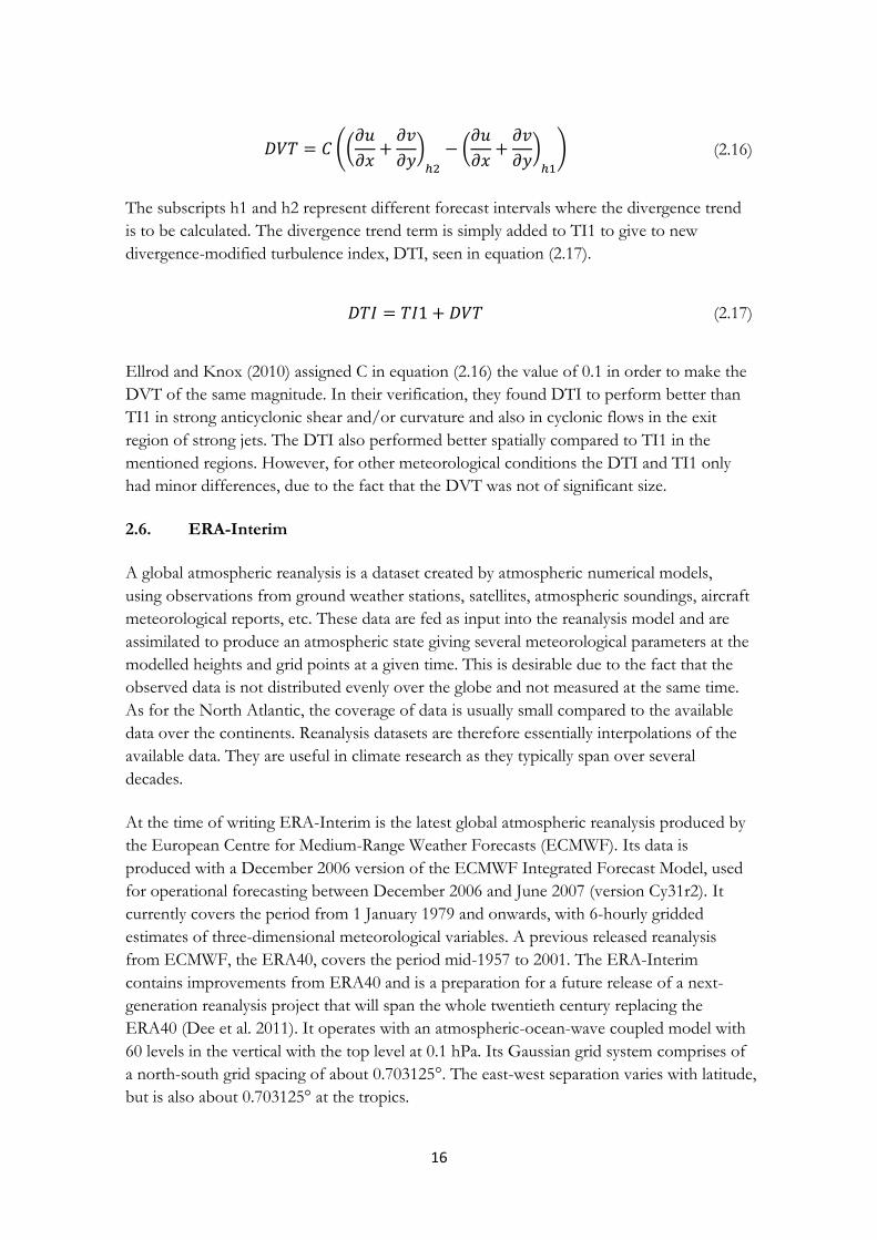
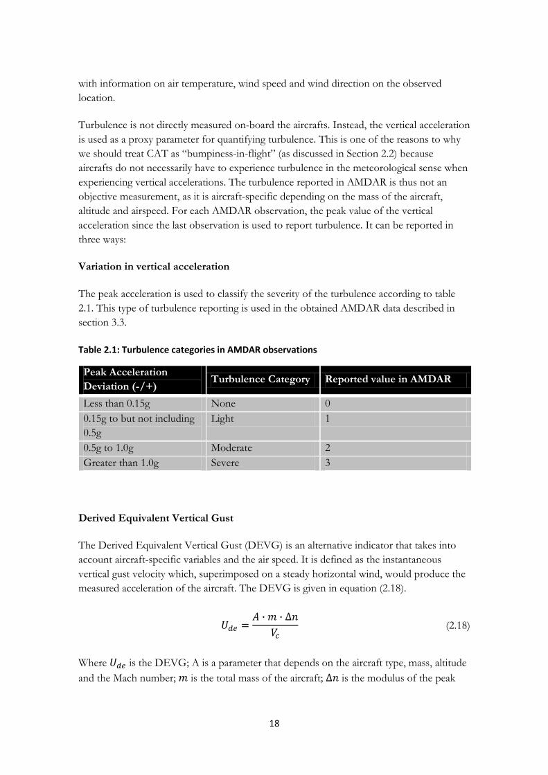
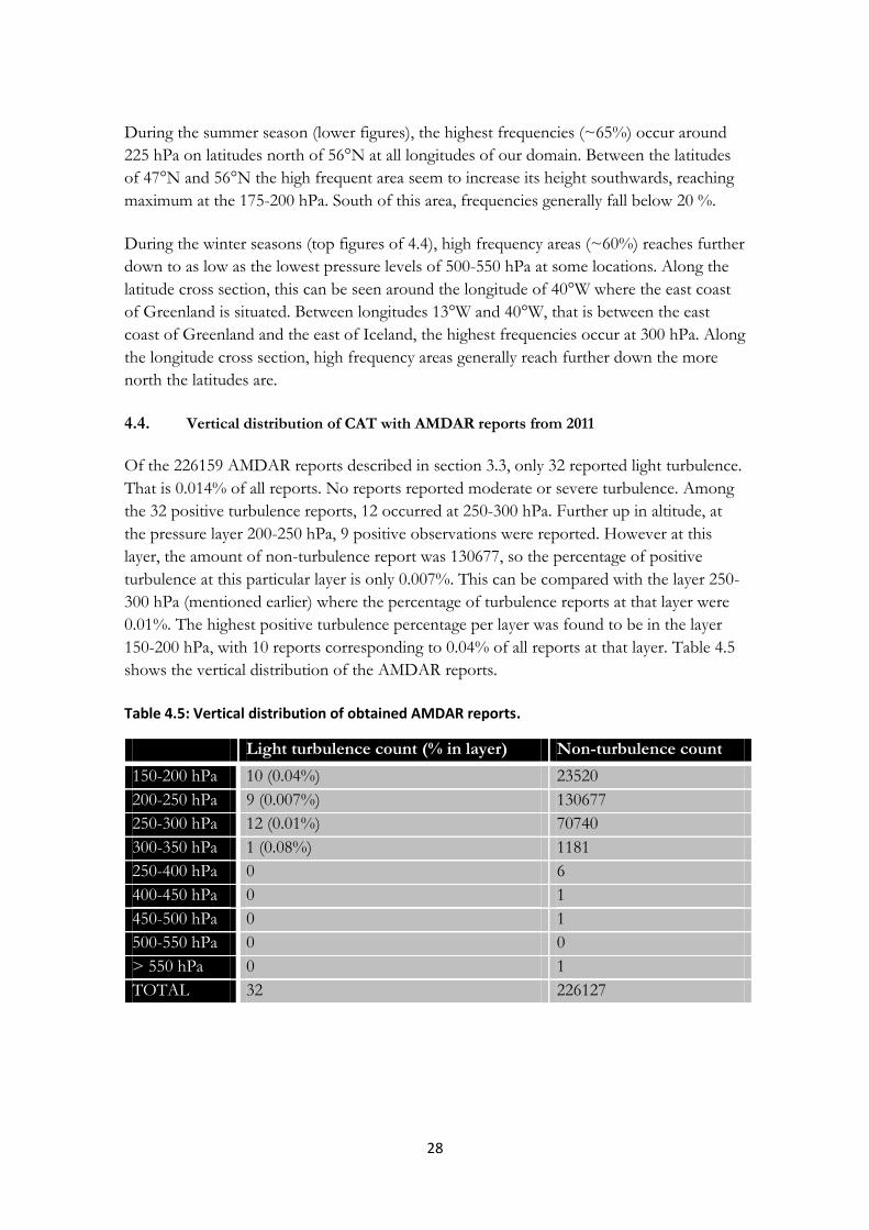

Appendix A Frequency plots of TI1
I
Figure A1 Frequency of TI1 values above the threshold value of 210-7
s-1
TI1 gt 210-7
s-1
Appendix A Frequency plots of TI1
II
Figure A2 Frequency of TI1 values above the threshold value of 1210
-7 s
-1
TI1 gt 1210-7
s-1
Appendix A Frequency plots of TI1
III
Figure A3 Frequency of TI1 values above the threshold value of 210
-7 s
-1 the 645degN latitude cross section
TI1 gt 210-7
s-11
along latitude 645degN
Appendix A Frequency plots of TI1
IV
Figure A4 Frequency of TI1 values above the threshold value of 1210-7
s-1
at the 645degN latitude cross section
TI1 gt 210-7
s-11
along latitude 645degN
Appendix A Frequency plots of TI1
V
Figure A5 Frequency of TI1 values above the threshold value of 210
-7 s
-1 at the 30degW longitude cross section
TI1 gt 210-7
s-1
along 30degW
Appendix A Frequency plots of TI1
VI
Figure A6 Frequency of TI1 values above the threshold value of 1210-7
s-1
at the 30degW longitude cross section
TI1 gt 1210-7
s-1
along 30degW
Appendix B Frequency plots of TI2
I
Figure B1 Frequency of TI2 values above the threshold value of 210-7
s-1
TI2 gt 210-7
s-1
Appendix B Frequency plots of TI2
II
Figure B2 Frequency of TI2 values above the threshold value of 1210
-7 s
-1
TI2 gt 1210-7
s-1
Appendix B Frequency plots of TI2
III
Figure B3 Frequency of TI2 values above the threshold value of 210-7
s-1
at the 645degN latitude cross section
TI2 gt 210-7
s-1
along 645degN
Appendix B Frequency plots of TI2
IV
Figure B4 Frequency of TI2 values above the threshold value of 1210-7
s-1
at the 645degN latitude cross section
TI2 gt 1210-7
s-1
along 645degN
Appendix B Frequency plots of TI2
V
Figure B5 Frequency of TI2 values above the threshold value of 210-7
s-1
at the 30degW longitude cross section
TI2 gt 210-7
s-1
along 30degW
Appendix B Frequency plots of TI2
VI
Figure B6 Frequency of TI2 values above the threshold value of 1210-7
s-1
at the 30degW longitude cross section
TI2 gt 1210-7
s-1
along 30degW
Tidigare utgivna publikationer i serien ISSN 1650-6553 Nr 1 Geomorphological mapping and hazard assessment of alpine areas in Vorarlberg Austria Marcus Gustavsson Nr 2 Verification of the Turbulence Index used at SMHI Stefan Bergman Nr 3 Forecasting the next dayrsquos maximum and minimum temperature in Vancouver Canada by using artificial neural network models Magnus Nilsson
Nr 4 The tectonic history of the Skyttorp-Vattholma fault zone south-central Sweden Anna Victoria Engstroumlm Nr 5 Investigation on Surface energy fluxes and their relationship to synoptic weather patterns on Storglaciaumlren northern Sweden Yvonne Kramer Nr 254 Malmmineralogisk undersoumlkning av Pb- Zn- Cu- och Ag-foumlrande kvartsgaringngar i Vaumlrmskogsomraringdet mellersta Vaumlrmland Christina Nysten February 2013 Nr 255 Kai XueThe Effects of Basal Friction and Basement Configuration on Deformation of Fold-and-Thrust Belts Insights from Analogue Modeling Kai Xue Mars 2013 Nr 256 Water quality in the Koga Irrigation Project Ethiopia A snapshot of general quality parametersVattenkvalitet i konstbevattningsprojektet i Koga Etiopien En oumlverblick av allmaumlnna kvalitetsparametrar Simon Eriksson Mars 2013
Nr 257 3D Processing of Seismic Data from the Ketzin CO2 Storage Site Germany Jawwad Ashraf Qureshi April 2013
Nr 258 Investigations of Manual and Satellite Observations of Snow in Jaumlraumlmauml (North Sweden) Daniel Pinto May 2013
Nr 259 Jaumlmfoumlrande studie av tvaring parameterskattningsmetoder i ett grundvattenmagasin Comparative study of two parameter estimation methods in a groundwater aquifer Stefan Eriksson May 2013
Nr 260 Case Study of Uncertainties Connected to Long-term Correction of Wind Observations Elisabeth Saarnak May 2013
Nr 261Variability and change in Koga reservoir volume Blue Nile Ethiopia Variabilitet och foumlraumlndring i Koga dammens vattenvolym Blaring Nilen Etiopien Benjamin Reynolds May 2013
Nr 262 Meteorological Investigation of Preconditions for Extreme-Scale Wind Turbines in Scandinavia Christoffer Hallgren May 2013 Nr 263 Application of the Reflection Seismic Method in Monitoring CO2 Injection in a Deep Saline Aquifer in the Baltic Sea Saba Joodaki May 2013

Appendix A Frequency plots of TI1
II
Figure A2 Frequency of TI1 values above the threshold value of 1210
-7 s
-1
TI1 gt 1210-7
s-1
Appendix A Frequency plots of TI1
III
Figure A3 Frequency of TI1 values above the threshold value of 210
-7 s
-1 the 645degN latitude cross section
TI1 gt 210-7
s-11
along latitude 645degN
Appendix A Frequency plots of TI1
IV
Figure A4 Frequency of TI1 values above the threshold value of 1210-7
s-1
at the 645degN latitude cross section
TI1 gt 210-7
s-11
along latitude 645degN
Appendix A Frequency plots of TI1
V
Figure A5 Frequency of TI1 values above the threshold value of 210
-7 s
-1 at the 30degW longitude cross section
TI1 gt 210-7
s-1
along 30degW
Appendix A Frequency plots of TI1
VI
Figure A6 Frequency of TI1 values above the threshold value of 1210-7
s-1
at the 30degW longitude cross section
TI1 gt 1210-7
s-1
along 30degW
Appendix B Frequency plots of TI2
I
Figure B1 Frequency of TI2 values above the threshold value of 210-7
s-1
TI2 gt 210-7
s-1
Appendix B Frequency plots of TI2
II
Figure B2 Frequency of TI2 values above the threshold value of 1210
-7 s
-1
TI2 gt 1210-7
s-1
Appendix B Frequency plots of TI2
III
Figure B3 Frequency of TI2 values above the threshold value of 210-7
s-1
at the 645degN latitude cross section
TI2 gt 210-7
s-1
along 645degN
Appendix B Frequency plots of TI2
IV
Figure B4 Frequency of TI2 values above the threshold value of 1210-7
s-1
at the 645degN latitude cross section
TI2 gt 1210-7
s-1
along 645degN
Appendix B Frequency plots of TI2
V
Figure B5 Frequency of TI2 values above the threshold value of 210-7
s-1
at the 30degW longitude cross section
TI2 gt 210-7
s-1
along 30degW
Appendix B Frequency plots of TI2
VI
Figure B6 Frequency of TI2 values above the threshold value of 1210-7
s-1
at the 30degW longitude cross section
TI2 gt 1210-7
s-1
along 30degW
Tidigare utgivna publikationer i serien ISSN 1650-6553 Nr 1 Geomorphological mapping and hazard assessment of alpine areas in Vorarlberg Austria Marcus Gustavsson Nr 2 Verification of the Turbulence Index used at SMHI Stefan Bergman Nr 3 Forecasting the next dayrsquos maximum and minimum temperature in Vancouver Canada by using artificial neural network models Magnus Nilsson
Nr 4 The tectonic history of the Skyttorp-Vattholma fault zone south-central Sweden Anna Victoria Engstroumlm Nr 5 Investigation on Surface energy fluxes and their relationship to synoptic weather patterns on Storglaciaumlren northern Sweden Yvonne Kramer Nr 254 Malmmineralogisk undersoumlkning av Pb- Zn- Cu- och Ag-foumlrande kvartsgaringngar i Vaumlrmskogsomraringdet mellersta Vaumlrmland Christina Nysten February 2013 Nr 255 Kai XueThe Effects of Basal Friction and Basement Configuration on Deformation of Fold-and-Thrust Belts Insights from Analogue Modeling Kai Xue Mars 2013 Nr 256 Water quality in the Koga Irrigation Project Ethiopia A snapshot of general quality parametersVattenkvalitet i konstbevattningsprojektet i Koga Etiopien En oumlverblick av allmaumlnna kvalitetsparametrar Simon Eriksson Mars 2013
Nr 257 3D Processing of Seismic Data from the Ketzin CO2 Storage Site Germany Jawwad Ashraf Qureshi April 2013
Nr 258 Investigations of Manual and Satellite Observations of Snow in Jaumlraumlmauml (North Sweden) Daniel Pinto May 2013
Nr 259 Jaumlmfoumlrande studie av tvaring parameterskattningsmetoder i ett grundvattenmagasin Comparative study of two parameter estimation methods in a groundwater aquifer Stefan Eriksson May 2013
Nr 260 Case Study of Uncertainties Connected to Long-term Correction of Wind Observations Elisabeth Saarnak May 2013
Nr 261Variability and change in Koga reservoir volume Blue Nile Ethiopia Variabilitet och foumlraumlndring i Koga dammens vattenvolym Blaring Nilen Etiopien Benjamin Reynolds May 2013
Nr 262 Meteorological Investigation of Preconditions for Extreme-Scale Wind Turbines in Scandinavia Christoffer Hallgren May 2013 Nr 263 Application of the Reflection Seismic Method in Monitoring CO2 Injection in a Deep Saline Aquifer in the Baltic Sea Saba Joodaki May 2013

Appendix A Frequency plots of TI1
III
Figure A3 Frequency of TI1 values above the threshold value of 210
-7 s
-1 the 645degN latitude cross section
TI1 gt 210-7
s-11
along latitude 645degN
Appendix A Frequency plots of TI1
IV
Figure A4 Frequency of TI1 values above the threshold value of 1210-7
s-1
at the 645degN latitude cross section
TI1 gt 210-7
s-11
along latitude 645degN
Appendix A Frequency plots of TI1
V
Figure A5 Frequency of TI1 values above the threshold value of 210
-7 s
-1 at the 30degW longitude cross section
TI1 gt 210-7
s-1
along 30degW
Appendix A Frequency plots of TI1
VI
Figure A6 Frequency of TI1 values above the threshold value of 1210-7
s-1
at the 30degW longitude cross section
TI1 gt 1210-7
s-1
along 30degW
Appendix B Frequency plots of TI2
I
Figure B1 Frequency of TI2 values above the threshold value of 210-7
s-1
TI2 gt 210-7
s-1
Appendix B Frequency plots of TI2
II
Figure B2 Frequency of TI2 values above the threshold value of 1210
-7 s
-1
TI2 gt 1210-7
s-1
Appendix B Frequency plots of TI2
III
Figure B3 Frequency of TI2 values above the threshold value of 210-7
s-1
at the 645degN latitude cross section
TI2 gt 210-7
s-1
along 645degN
Appendix B Frequency plots of TI2
IV
Figure B4 Frequency of TI2 values above the threshold value of 1210-7
s-1
at the 645degN latitude cross section
TI2 gt 1210-7
s-1
along 645degN
Appendix B Frequency plots of TI2
V
Figure B5 Frequency of TI2 values above the threshold value of 210-7
s-1
at the 30degW longitude cross section
TI2 gt 210-7
s-1
along 30degW
Appendix B Frequency plots of TI2
VI
Figure B6 Frequency of TI2 values above the threshold value of 1210-7
s-1
at the 30degW longitude cross section
TI2 gt 1210-7
s-1
along 30degW
Tidigare utgivna publikationer i serien ISSN 1650-6553 Nr 1 Geomorphological mapping and hazard assessment of alpine areas in Vorarlberg Austria Marcus Gustavsson Nr 2 Verification of the Turbulence Index used at SMHI Stefan Bergman Nr 3 Forecasting the next dayrsquos maximum and minimum temperature in Vancouver Canada by using artificial neural network models Magnus Nilsson
Nr 4 The tectonic history of the Skyttorp-Vattholma fault zone south-central Sweden Anna Victoria Engstroumlm Nr 5 Investigation on Surface energy fluxes and their relationship to synoptic weather patterns on Storglaciaumlren northern Sweden Yvonne Kramer Nr 254 Malmmineralogisk undersoumlkning av Pb- Zn- Cu- och Ag-foumlrande kvartsgaringngar i Vaumlrmskogsomraringdet mellersta Vaumlrmland Christina Nysten February 2013 Nr 255 Kai XueThe Effects of Basal Friction and Basement Configuration on Deformation of Fold-and-Thrust Belts Insights from Analogue Modeling Kai Xue Mars 2013 Nr 256 Water quality in the Koga Irrigation Project Ethiopia A snapshot of general quality parametersVattenkvalitet i konstbevattningsprojektet i Koga Etiopien En oumlverblick av allmaumlnna kvalitetsparametrar Simon Eriksson Mars 2013
Nr 257 3D Processing of Seismic Data from the Ketzin CO2 Storage Site Germany Jawwad Ashraf Qureshi April 2013
Nr 258 Investigations of Manual and Satellite Observations of Snow in Jaumlraumlmauml (North Sweden) Daniel Pinto May 2013
Nr 259 Jaumlmfoumlrande studie av tvaring parameterskattningsmetoder i ett grundvattenmagasin Comparative study of two parameter estimation methods in a groundwater aquifer Stefan Eriksson May 2013
Nr 260 Case Study of Uncertainties Connected to Long-term Correction of Wind Observations Elisabeth Saarnak May 2013
Nr 261Variability and change in Koga reservoir volume Blue Nile Ethiopia Variabilitet och foumlraumlndring i Koga dammens vattenvolym Blaring Nilen Etiopien Benjamin Reynolds May 2013
Nr 262 Meteorological Investigation of Preconditions for Extreme-Scale Wind Turbines in Scandinavia Christoffer Hallgren May 2013 Nr 263 Application of the Reflection Seismic Method in Monitoring CO2 Injection in a Deep Saline Aquifer in the Baltic Sea Saba Joodaki May 2013

Appendix A Frequency plots of TI1
IV
Figure A4 Frequency of TI1 values above the threshold value of 1210-7
s-1
at the 645degN latitude cross section
TI1 gt 210-7
s-11
along latitude 645degN
Appendix A Frequency plots of TI1
V
Figure A5 Frequency of TI1 values above the threshold value of 210
-7 s
-1 at the 30degW longitude cross section
TI1 gt 210-7
s-1
along 30degW
Appendix A Frequency plots of TI1
VI
Figure A6 Frequency of TI1 values above the threshold value of 1210-7
s-1
at the 30degW longitude cross section
TI1 gt 1210-7
s-1
along 30degW
Appendix B Frequency plots of TI2
I
Figure B1 Frequency of TI2 values above the threshold value of 210-7
s-1
TI2 gt 210-7
s-1
Appendix B Frequency plots of TI2
II
Figure B2 Frequency of TI2 values above the threshold value of 1210
-7 s
-1
TI2 gt 1210-7
s-1
Appendix B Frequency plots of TI2
III
Figure B3 Frequency of TI2 values above the threshold value of 210-7
s-1
at the 645degN latitude cross section
TI2 gt 210-7
s-1
along 645degN
Appendix B Frequency plots of TI2
IV
Figure B4 Frequency of TI2 values above the threshold value of 1210-7
s-1
at the 645degN latitude cross section
TI2 gt 1210-7
s-1
along 645degN
Appendix B Frequency plots of TI2
V
Figure B5 Frequency of TI2 values above the threshold value of 210-7
s-1
at the 30degW longitude cross section
TI2 gt 210-7
s-1
along 30degW
Appendix B Frequency plots of TI2
VI
Figure B6 Frequency of TI2 values above the threshold value of 1210-7
s-1
at the 30degW longitude cross section
TI2 gt 1210-7
s-1
along 30degW
Tidigare utgivna publikationer i serien ISSN 1650-6553 Nr 1 Geomorphological mapping and hazard assessment of alpine areas in Vorarlberg Austria Marcus Gustavsson Nr 2 Verification of the Turbulence Index used at SMHI Stefan Bergman Nr 3 Forecasting the next dayrsquos maximum and minimum temperature in Vancouver Canada by using artificial neural network models Magnus Nilsson
Nr 4 The tectonic history of the Skyttorp-Vattholma fault zone south-central Sweden Anna Victoria Engstroumlm Nr 5 Investigation on Surface energy fluxes and their relationship to synoptic weather patterns on Storglaciaumlren northern Sweden Yvonne Kramer Nr 254 Malmmineralogisk undersoumlkning av Pb- Zn- Cu- och Ag-foumlrande kvartsgaringngar i Vaumlrmskogsomraringdet mellersta Vaumlrmland Christina Nysten February 2013 Nr 255 Kai XueThe Effects of Basal Friction and Basement Configuration on Deformation of Fold-and-Thrust Belts Insights from Analogue Modeling Kai Xue Mars 2013 Nr 256 Water quality in the Koga Irrigation Project Ethiopia A snapshot of general quality parametersVattenkvalitet i konstbevattningsprojektet i Koga Etiopien En oumlverblick av allmaumlnna kvalitetsparametrar Simon Eriksson Mars 2013
Nr 257 3D Processing of Seismic Data from the Ketzin CO2 Storage Site Germany Jawwad Ashraf Qureshi April 2013
Nr 258 Investigations of Manual and Satellite Observations of Snow in Jaumlraumlmauml (North Sweden) Daniel Pinto May 2013
Nr 259 Jaumlmfoumlrande studie av tvaring parameterskattningsmetoder i ett grundvattenmagasin Comparative study of two parameter estimation methods in a groundwater aquifer Stefan Eriksson May 2013
Nr 260 Case Study of Uncertainties Connected to Long-term Correction of Wind Observations Elisabeth Saarnak May 2013
Nr 261Variability and change in Koga reservoir volume Blue Nile Ethiopia Variabilitet och foumlraumlndring i Koga dammens vattenvolym Blaring Nilen Etiopien Benjamin Reynolds May 2013
Nr 262 Meteorological Investigation of Preconditions for Extreme-Scale Wind Turbines in Scandinavia Christoffer Hallgren May 2013 Nr 263 Application of the Reflection Seismic Method in Monitoring CO2 Injection in a Deep Saline Aquifer in the Baltic Sea Saba Joodaki May 2013

Appendix A Frequency plots of TI1
V
Figure A5 Frequency of TI1 values above the threshold value of 210
-7 s
-1 at the 30degW longitude cross section
TI1 gt 210-7
s-1
along 30degW
Appendix A Frequency plots of TI1
VI
Figure A6 Frequency of TI1 values above the threshold value of 1210-7
s-1
at the 30degW longitude cross section
TI1 gt 1210-7
s-1
along 30degW
Appendix B Frequency plots of TI2
I
Figure B1 Frequency of TI2 values above the threshold value of 210-7
s-1
TI2 gt 210-7
s-1
Appendix B Frequency plots of TI2
II
Figure B2 Frequency of TI2 values above the threshold value of 1210
-7 s
-1
TI2 gt 1210-7
s-1
Appendix B Frequency plots of TI2
III
Figure B3 Frequency of TI2 values above the threshold value of 210-7
s-1
at the 645degN latitude cross section
TI2 gt 210-7
s-1
along 645degN
Appendix B Frequency plots of TI2
IV
Figure B4 Frequency of TI2 values above the threshold value of 1210-7
s-1
at the 645degN latitude cross section
TI2 gt 1210-7
s-1
along 645degN
Appendix B Frequency plots of TI2
V
Figure B5 Frequency of TI2 values above the threshold value of 210-7
s-1
at the 30degW longitude cross section
TI2 gt 210-7
s-1
along 30degW
Appendix B Frequency plots of TI2
VI
Figure B6 Frequency of TI2 values above the threshold value of 1210-7
s-1
at the 30degW longitude cross section
TI2 gt 1210-7
s-1
along 30degW
Tidigare utgivna publikationer i serien ISSN 1650-6553 Nr 1 Geomorphological mapping and hazard assessment of alpine areas in Vorarlberg Austria Marcus Gustavsson Nr 2 Verification of the Turbulence Index used at SMHI Stefan Bergman Nr 3 Forecasting the next dayrsquos maximum and minimum temperature in Vancouver Canada by using artificial neural network models Magnus Nilsson
Nr 4 The tectonic history of the Skyttorp-Vattholma fault zone south-central Sweden Anna Victoria Engstroumlm Nr 5 Investigation on Surface energy fluxes and their relationship to synoptic weather patterns on Storglaciaumlren northern Sweden Yvonne Kramer Nr 254 Malmmineralogisk undersoumlkning av Pb- Zn- Cu- och Ag-foumlrande kvartsgaringngar i Vaumlrmskogsomraringdet mellersta Vaumlrmland Christina Nysten February 2013 Nr 255 Kai XueThe Effects of Basal Friction and Basement Configuration on Deformation of Fold-and-Thrust Belts Insights from Analogue Modeling Kai Xue Mars 2013 Nr 256 Water quality in the Koga Irrigation Project Ethiopia A snapshot of general quality parametersVattenkvalitet i konstbevattningsprojektet i Koga Etiopien En oumlverblick av allmaumlnna kvalitetsparametrar Simon Eriksson Mars 2013
Nr 257 3D Processing of Seismic Data from the Ketzin CO2 Storage Site Germany Jawwad Ashraf Qureshi April 2013
Nr 258 Investigations of Manual and Satellite Observations of Snow in Jaumlraumlmauml (North Sweden) Daniel Pinto May 2013
Nr 259 Jaumlmfoumlrande studie av tvaring parameterskattningsmetoder i ett grundvattenmagasin Comparative study of two parameter estimation methods in a groundwater aquifer Stefan Eriksson May 2013
Nr 260 Case Study of Uncertainties Connected to Long-term Correction of Wind Observations Elisabeth Saarnak May 2013
Nr 261Variability and change in Koga reservoir volume Blue Nile Ethiopia Variabilitet och foumlraumlndring i Koga dammens vattenvolym Blaring Nilen Etiopien Benjamin Reynolds May 2013
Nr 262 Meteorological Investigation of Preconditions for Extreme-Scale Wind Turbines in Scandinavia Christoffer Hallgren May 2013 Nr 263 Application of the Reflection Seismic Method in Monitoring CO2 Injection in a Deep Saline Aquifer in the Baltic Sea Saba Joodaki May 2013

Appendix A Frequency plots of TI1
VI
Figure A6 Frequency of TI1 values above the threshold value of 1210-7
s-1
at the 30degW longitude cross section
TI1 gt 1210-7
s-1
along 30degW
Appendix B Frequency plots of TI2
I
Figure B1 Frequency of TI2 values above the threshold value of 210-7
s-1
TI2 gt 210-7
s-1
Appendix B Frequency plots of TI2
II
Figure B2 Frequency of TI2 values above the threshold value of 1210
-7 s
-1
TI2 gt 1210-7
s-1
Appendix B Frequency plots of TI2
III
Figure B3 Frequency of TI2 values above the threshold value of 210-7
s-1
at the 645degN latitude cross section
TI2 gt 210-7
s-1
along 645degN
Appendix B Frequency plots of TI2
IV
Figure B4 Frequency of TI2 values above the threshold value of 1210-7
s-1
at the 645degN latitude cross section
TI2 gt 1210-7
s-1
along 645degN
Appendix B Frequency plots of TI2
V
Figure B5 Frequency of TI2 values above the threshold value of 210-7
s-1
at the 30degW longitude cross section
TI2 gt 210-7
s-1
along 30degW
Appendix B Frequency plots of TI2
VI
Figure B6 Frequency of TI2 values above the threshold value of 1210-7
s-1
at the 30degW longitude cross section
TI2 gt 1210-7
s-1
along 30degW
Tidigare utgivna publikationer i serien ISSN 1650-6553 Nr 1 Geomorphological mapping and hazard assessment of alpine areas in Vorarlberg Austria Marcus Gustavsson Nr 2 Verification of the Turbulence Index used at SMHI Stefan Bergman Nr 3 Forecasting the next dayrsquos maximum and minimum temperature in Vancouver Canada by using artificial neural network models Magnus Nilsson
Nr 4 The tectonic history of the Skyttorp-Vattholma fault zone south-central Sweden Anna Victoria Engstroumlm Nr 5 Investigation on Surface energy fluxes and their relationship to synoptic weather patterns on Storglaciaumlren northern Sweden Yvonne Kramer Nr 254 Malmmineralogisk undersoumlkning av Pb- Zn- Cu- och Ag-foumlrande kvartsgaringngar i Vaumlrmskogsomraringdet mellersta Vaumlrmland Christina Nysten February 2013 Nr 255 Kai XueThe Effects of Basal Friction and Basement Configuration on Deformation of Fold-and-Thrust Belts Insights from Analogue Modeling Kai Xue Mars 2013 Nr 256 Water quality in the Koga Irrigation Project Ethiopia A snapshot of general quality parametersVattenkvalitet i konstbevattningsprojektet i Koga Etiopien En oumlverblick av allmaumlnna kvalitetsparametrar Simon Eriksson Mars 2013
Nr 257 3D Processing of Seismic Data from the Ketzin CO2 Storage Site Germany Jawwad Ashraf Qureshi April 2013
Nr 258 Investigations of Manual and Satellite Observations of Snow in Jaumlraumlmauml (North Sweden) Daniel Pinto May 2013
Nr 259 Jaumlmfoumlrande studie av tvaring parameterskattningsmetoder i ett grundvattenmagasin Comparative study of two parameter estimation methods in a groundwater aquifer Stefan Eriksson May 2013
Nr 260 Case Study of Uncertainties Connected to Long-term Correction of Wind Observations Elisabeth Saarnak May 2013
Nr 261Variability and change in Koga reservoir volume Blue Nile Ethiopia Variabilitet och foumlraumlndring i Koga dammens vattenvolym Blaring Nilen Etiopien Benjamin Reynolds May 2013
Nr 262 Meteorological Investigation of Preconditions for Extreme-Scale Wind Turbines in Scandinavia Christoffer Hallgren May 2013 Nr 263 Application of the Reflection Seismic Method in Monitoring CO2 Injection in a Deep Saline Aquifer in the Baltic Sea Saba Joodaki May 2013

Appendix B Frequency plots of TI2
VI
Figure B6 Frequency of TI2 values above the threshold value of 1210-7
s-1
at the 30degW longitude cross section
TI2 gt 1210-7
s-1
along 30degW
Tidigare utgivna publikationer i serien ISSN 1650-6553 Nr 1 Geomorphological mapping and hazard assessment of alpine areas in Vorarlberg Austria Marcus Gustavsson Nr 2 Verification of the Turbulence Index used at SMHI Stefan Bergman Nr 3 Forecasting the next dayrsquos maximum and minimum temperature in Vancouver Canada by using artificial neural network models Magnus Nilsson
Nr 4 The tectonic history of the Skyttorp-Vattholma fault zone south-central Sweden Anna Victoria Engstroumlm Nr 5 Investigation on Surface energy fluxes and their relationship to synoptic weather patterns on Storglaciaumlren northern Sweden Yvonne Kramer Nr 254 Malmmineralogisk undersoumlkning av Pb- Zn- Cu- och Ag-foumlrande kvartsgaringngar i Vaumlrmskogsomraringdet mellersta Vaumlrmland Christina Nysten February 2013 Nr 255 Kai XueThe Effects of Basal Friction and Basement Configuration on Deformation of Fold-and-Thrust Belts Insights from Analogue Modeling Kai Xue Mars 2013 Nr 256 Water quality in the Koga Irrigation Project Ethiopia A snapshot of general quality parametersVattenkvalitet i konstbevattningsprojektet i Koga Etiopien En oumlverblick av allmaumlnna kvalitetsparametrar Simon Eriksson Mars 2013
Nr 257 3D Processing of Seismic Data from the Ketzin CO2 Storage Site Germany Jawwad Ashraf Qureshi April 2013
Nr 258 Investigations of Manual and Satellite Observations of Snow in Jaumlraumlmauml (North Sweden) Daniel Pinto May 2013
Nr 259 Jaumlmfoumlrande studie av tvaring parameterskattningsmetoder i ett grundvattenmagasin Comparative study of two parameter estimation methods in a groundwater aquifer Stefan Eriksson May 2013
Nr 260 Case Study of Uncertainties Connected to Long-term Correction of Wind Observations Elisabeth Saarnak May 2013
Nr 261Variability and change in Koga reservoir volume Blue Nile Ethiopia Variabilitet och foumlraumlndring i Koga dammens vattenvolym Blaring Nilen Etiopien Benjamin Reynolds May 2013
Nr 262 Meteorological Investigation of Preconditions for Extreme-Scale Wind Turbines in Scandinavia Christoffer Hallgren May 2013 Nr 263 Application of the Reflection Seismic Method in Monitoring CO2 Injection in a Deep Saline Aquifer in the Baltic Sea Saba Joodaki May 2013