Embed Size (px)
Citation preview
Less is More: Selecting Sources Wisely for Integration
Xin Luna DongAT&T [email protected]
Barna SahaAT&T Labs-Research
Divesh SrivastavaAT&T Labs-Research
ABSTRACTWe are often thrilled by the abundance of information surroundingus and wish to integrate data from as many sources as possible toimprove the quality of the integrated data. However, understand-ing, analyzing, and using these data are often hard. Too much datacan introduce a huge integration cost, such as expenses for purchas-ing data and resources for integration and cleaning. Furthermore,including low-quality data can even deteriorate the quality of inte-gration results instead of bringing the desired quality gain. Thus,“the more the better” does not always hold for information and of-ten “less is more”.
In this paper, we study how to select a subset of sources beforeintegration such that we can balance the quality of integrated dataand integration cost. Inspired by the Marginalism principle in eco-nomic theory, we wish to stop integrating a new source when themarginal gain, often a function of improved integration quality, isless than the marginal cost, associated with data-purchase expenseand integration resources. As a first step towards this goal, we fo-cus on data fusion tasks, where the goal is to resolve conflicts fromdifferent sources. We propose a randomized solution for selectingsources for fusion and show empirically its effectiveness and scal-ability on both real-world data and synthetic data.
1. INTRODUCTION
1.1 MotivationThe Information Era has witnessed not only a huge volume of
data, but also a huge number of sources or data feeds from web-sites, Twitter, blogs, online social networks, collaborative annota-tions, social bookmarking, data markets, and so on. The abundanceof useful information surrounding us and the advantage of easy datasharing have made it possible for data warehousing and integrationsystems to improve the quality of the integrated data. For exam-ple, with more sources, we can increase the coverage of the inte-grated data; in the presence of inconsistency, we can improve cor-rectness of the integrated data by leveraging the collective wisdom.Such quality improvement allows for more advanced data analysisand can bring a big gain. However, we also need to bear in mind
that data collection and integration come with a cost. First, manydata sources, such as GeoLytics for demographic data1, WDT forweather data2, GeoEye for satellite imagery3, American BusinessDatabase for business listings4, charge for their data. Second, evenfor sources that are free, integration requires spending resourceson mapping heterogeneous data items, resolving conflicts, cleaningthe data, and so on. Such costs can also be huge. Actually, thecost of integrating some sources may not be worthwhile if the gainis limited, especially in the presence of redundant data and low-quality data. We next use a real-world example to illustrate this.
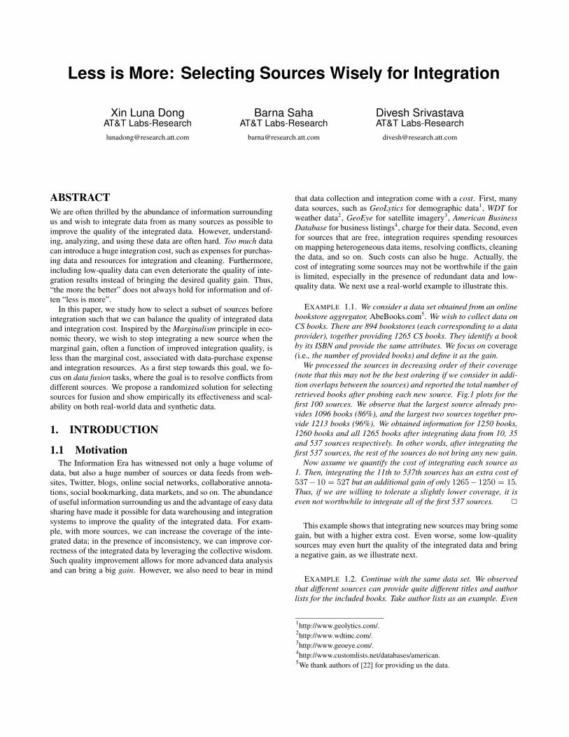
EXAMPLE 1.1. We consider a data set obtained from an onlinebookstore aggregator, AbeBooks.com5. We wish to collect data onCS books. There are 894 bookstores (each corresponding to a dataprovider), together providing 1265 CS books. They identify a bookby its ISBN and provide the same attributes. We focus on coverage(i.e., the number of provided books) and define it as the gain.
We processed the sources in decreasing order of their coverage(note that this may not be the best ordering if we consider in addi-tion overlaps between the sources) and reported the total number ofretrieved books after probing each new source. Fig.1 plots for thefirst 100 sources. We observe that the largest source already pro-vides 1096 books (86%), and the largest two sources together pro-vide 1213 books (96%). We obtained information for 1250 books,1260 books and all 1265 books after integrating data from 10, 35and 537 sources respectively. In other words, after integrating thefirst 537 sources, the rest of the sources do not bring any new gain.
Now assume we quantify the cost of integrating each source as1. Then, integrating the 11th to 537th sources has an extra cost of537−10 = 527 but an additional gain of only 1265−1250 = 15.Thus, if we are willing to tolerate a slightly lower coverage, it iseven not worthwhile to integrate all of the first 537 sources. 2
This example shows that integrating new sources may bring somegain, but with a higher extra cost. Even worse, some low-qualitysources may even hurt the quality of the integrated data and bringa negative gain, as we illustrate next.
EXAMPLE 1.2. Continue with the same data set. We observedthat different sources can provide quite different titles and authorlists for the included books. Take author lists as an example. Even
1http://www.geolytics.com/.2http://www.wdtinc.com/.3http://www.geoeye.com/.4http://www.customlists.net/databases/american.5We thank authors of [22] for providing us the data.
1000
1050
1100
1150
1200
1250
1300
0 25 50 75 100
#(R
etu
rne
d b
oo
ks)
#Sources
Coverage of Results as We Add Sources
Figure 1: Coverage of results.
0 10 20 30 40 50 60 70 80 90
100
0
50
10
0
15
0
20
0
25
0
30
0
35
0
40
0
45
0
50
0
55
0
60
0
65
0
70
0
75
0
80
0
85
0
Gai
n=#
(Co
rre
ct a
uth
ors
)
#Sources
Number of Correctly Returned Authors as We Add Sources
#(Returned books) Vote Accu Cost
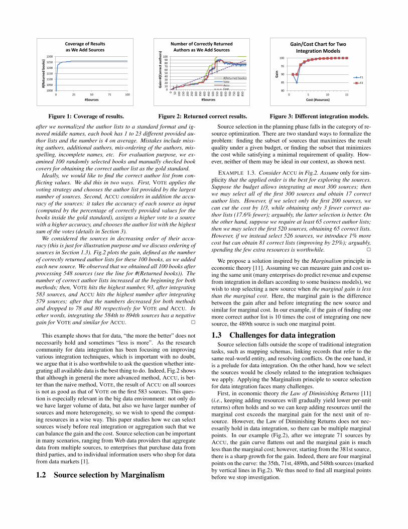
Figure 2: Returned correct results.
80
85
90
95
100
0 5 10 15
Gai
n
Cost (#sources)
Gain/Cost Chart for Two Integration Models
F1
F2
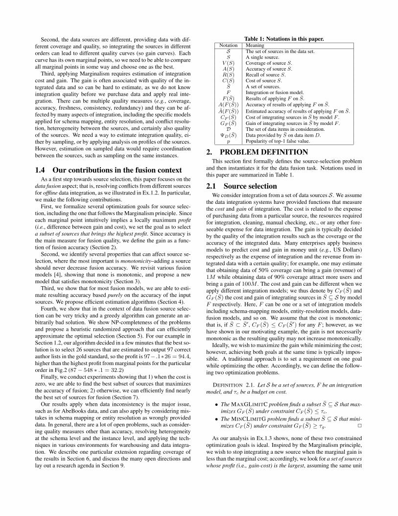
Figure 3: Different integration models.
after we normalized the author lists to a standard format and ig-nored middle names, each book has 1 to 23 different provided au-thor lists and the number is 4 on average. Mistakes include miss-ing authors, additional authors, mis-ordering of the authors, mis-spelling, incomplete names, etc. For evaluation purpose, we ex-amined 100 randomly selected books and manually checked bookcovers for obtaining the correct author list as the gold standard.
Ideally, we would like to find the correct author list from con-flicting values. We did this in two ways. First, VOTE applies thevoting strategy and chooses the author list provided by the largestnumber of sources. Second, ACCU considers in addition the accu-racy of the sources: it takes the accuracy of each source as input(computed by the percentage of correctly provided values for thebooks inside the gold standard), assigns a higher vote to a sourcewith a higher accuracy, and chooses the author list with the highestsum of the votes (details in Section 3).
We considered the sources in decreasing order of their accu-racy (this is just for illustration purpose and we discuss ordering ofsources in Section 1.3). Fig.2 plots the gain, defined as the numberof correctly returned author lists for these 100 books, as we addedeach new source. We observed that we obtained all 100 books afterprocessing 548 sources (see the line for #(Returned books)). Thenumber of correct author lists increased at the beginning for bothmethods; then, VOTE hits the highest number, 93, after integrating583 sources, and ACCU hits the highest number after integrating579 sources; after that the numbers decreased for both methodsand dropped to 78 and 80 respectively for VOTE and ACCU. Inother words, integrating the 584th to 894th sources has a negativegain for VOTE and similar for ACCU. 2
This example shows that for data, “the more the better” does notnecessarily hold and sometimes “less is more”. As the researchcommunity for data integration has been focusing on improvingvarious integration techniques, which is important with no doubt,we argue that it is also worthwhile to ask the question whether inte-grating all available data is the best thing to do. Indeed, Fig.2 showsthat although in general the more advanced method, ACCU, is bet-ter than the naive method, VOTE, the result of ACCU on all sourcesis not as good as that of VOTE on the first 583 sources. This ques-tion is especially relevant in the big data environment: not only dowe have larger volume of data, but also we have larger number ofsources and more heterogeneity, so we wish to spend the comput-ing resources in a wise way. This paper studies how we can selectsources wisely before real integration or aggregation such that wecan balance the gain and the cost. Source selection can be importantin many scenarios, ranging from Web data providers that aggregatedata from multiple sources, to enterprises that purchase data fromthird parties, and to individual information users who shop for datafrom data markets [1].
1.2 Source selection by Marginalism
Source selection in the planning phase falls in the category of re-source optimization. There are two standard ways to formalize theproblem: finding the subset of sources that maximizes the resultquality under a given budget, or finding the subset that minimizesthe cost while satisfying a minimal requirement of quality. How-ever, neither of them may be ideal in our context, as shown next.
EXAMPLE 1.3. Consider ACCU in Fig.2. Assume only for sim-plicity that the applied order is the best for exploring the sources.Suppose the budget allows integrating at most 300 sources; thenwe may select all of the first 300 sources and obtain 17 correctauthor lists. However, if we select only the first 200 sources, wecan cut the cost by 1/3, while obtaining only 3 fewer correct au-thor lists (17.6% fewer); arguably, the latter selection is better. Onthe other hand, suppose we require at least 65 correct author lists;then we may select the first 520 sources, obtaining 65 correct lists.However, if we instead select 526 sources, we introduce 1% morecost but can obtain 81 correct lists (improving by 25%); arguably,spending the few extra resources is worthwhile. 2
We propose a solution inspired by the Marginalism principle ineconomic theory [11]. Assuming we can measure gain and cost us-ing the same unit (many enterprises do predict revenue and expensefrom integration in dollars according to some business models), wewish to stop selecting a new source when the marginal gain is lessthan the marginal cost. Here, the marginal gain is the differencebetween the gain after and before integrating the new source andsimilar for marginal cost. In our example, if the gain of finding onemore correct author list is 10 times the cost of integrating one newsource, the 489th source is such one marginal point.
1.3 Challenges for data integrationSource selection falls outside the scope of traditional integration
tasks, such as mapping schemas, linking records that refer to thesame real-world entity, and resolving conflicts. On the one hand, itis a prelude for data integration. On the other hand, how we selectthe sources would be closely related to the integration techniqueswe apply. Applying the Marginalism principle to source selectionfor data integration faces many challenges.
First, in economic theory the Law of Diminishing Returns [11](i.e., keeping adding resources will gradually yield lower per-unitreturns) often holds and so we can keep adding resources until themarginal cost exceeds the marginal gain for the next unit of re-source. However, the Law of Diminishing Returns does not nec-essarily hold in data integration, so there can be multiple marginalpoints. In our example (Fig.2), after we integrate 71 sources byACCU, the gain curve flattens out and the marginal gain is muchless than the marginal cost; however, starting from the 381st source,there is a sharp growth for the gain. Indeed, there are four marginalpoints on the curve: the 35th, 71st, 489th, and 548th sources (markedby vertical lines in Fig.2). We thus need to find all marginal pointsbefore we stop investigation.
Second, the data sources are different, providing data with dif-ferent coverage and quality, so integrating the sources in differentorders can lead to different quality curves (so gain curves). Eachcurve has its own marginal points, so we need to be able to compareall marginal points in some way and choose one as the best.
Third, applying Marginalism requires estimation of integrationcost and gain. The gain is often associated with quality of the in-tegrated data and so can be hard to estimate, as we do not knowintegration quality before we purchase data and apply real inte-gration. There can be multiple quality measures (e.g., coverage,accuracy, freshness, consistency, redundancy) and they can be af-fected by many aspects of integration, including the specific modelsapplied for schema mapping, entity resolution, and conflict resolu-tion, heterogeneity between the sources, and certainly also qualityof the sources. We need a way to estimate integration quality, ei-ther by sampling, or by applying analysis on profiles of the sources.However, estimation on sampled data would require coordinationbetween the sources, such as sampling on the same instances.
1.4 Our contributions in the fusion contextAs a first step towards source selection, this paper focuses on the
data fusion aspect; that is, resolving conflicts from different sourcesfor offline data integration, as we illustrated in Ex.1.2. In particular,we make the following contributions.
First, we formalize several optimization goals for source selec-tion, including the one that follows the Marginalism principle. Sinceeach marginal point intuitively implies a locally maximum profit(i.e., difference between gain and cost), we set the goal as to selecta subset of sources that brings the highest profit. Since accuracy isthe main measure for fusion quality, we define the gain as a func-tion of fusion accuracy (Section 2).
Second, we identify several properties that can affect source se-lection, where the most important is monotonicity–adding a sourceshould never decrease fusion accuracy. We revisit various fusionmodels [4], showing that none is monotonic, and propose a newmodel that satisfies monotonicity (Section 3).
Third, we show that for most fusion models, we are able to esti-mate resulting accuracy based purely on the accuracy of the inputsources. We propose efficient estimation algorithms (Section 4).
Fourth, we show that in the context of data fusion source selec-tion can be very tricky and a greedy algorithm can generate an ar-bitrarily bad solution. We show NP-completeness of the problemsand propose a heuristic randomized approach that can efficientlyapproximate the optimal selection (Section 5). For our example inSection 1.2, our algorithm decided in a few minutes that the best so-lution is to select 26 sources that are estimated to output 97 correctauthor lists in the gold standard, so the profit is 97− .1∗26 = 94.4,higher than the highest profit from marginal points for the particularorder in Fig.2 (87− 548 ∗ .1 = 32.2)
Finally, we conduct experiments showing that 1) when the cost iszero, we are able to find the best subset of sources that maximizesthe accuracy of fusion; 2) otherwise, we can efficiently find nearlythe best set of sources for fusion (Section 7).
Our results apply when data inconsistency is the major issue,such as for AbeBooks data, and can also apply by considering mis-takes in schema mapping or entity resolution as wrongly provideddata. In general, there are a lot of open problems, such as consider-ing quality measures other than accuracy, resolving heterogeneityat the schema level and the instance level, and applying the tech-niques in various environments for warehousing and data integra-tion. We describe one particular extension regarding coverage ofthe results in Section 6, and discuss the many open directions andlay out a research agenda in Section 9.
Table 1: Notations in this paper.Notation MeaningS The set of sources in the data set.S A single source.
V (S) Coverage of source S.A(S) Accuracy of source S.R(S) Recall of source S.C(S) Cost of source S.
S A set of sources.F Integration or fusion model.
F (S) Results of applying F on S.A(F (S)) Accuracy of results of applying F on S.A(F (S)) Estimated accuracy of results of applying F on S.CF (S) Cost of integrating sources in S by model F .GF (S) Gain of integrating sources in S by model F .D The set of data items in consideration.
ΨD(S) Data provided by S on data item D.p Popularity of top-1 false value.
2. PROBLEM DEFINITIONThis section first formally defines the source-selection problem
and then instantiates it for the data fusion task. Notations used inthis paper are summarized in Table 1.
2.1 Source selectionWe consider integration from a set of data sources S. We assume
the data integration systems have provided functions that measurethe cost and gain of integration. The cost is related to the expenseof purchasing data from a particular source, the resources requiredfor integration, cleaning, manual checking, etc., or any other fore-seeable expense for data integration. The gain is typically decidedby the quality of the integration results such as the coverage or theaccuracy of the integrated data. Many enterprises apply businessmodels to predict cost and gain in money unit (e.g., US Dollars)respectively as the expense of integration and the revenue from in-tegrated data with a certain quality; for example, one may estimatethat obtaining data of 50% coverage can bring a gain (revenue) of1M while obtaining data of 90% coverage attract more users andbring a gain of 100M . The cost and gain can be different when weapply different integration models; we thus denote by CF (S) andGF (S) the cost and gain of integrating sources in S ⊆ S by modelF respectively. Here, F can be one or a set of integration modelsincluding schema-mapping models, entity-resolution models, data-fusion models, and so on. We assume that the cost is monotonic;that is, if S ⊂ S′, CF (S) ≤ CF (S′) for any F ; however, as wehave shown in our motivating example, the gain is not necessarilymonotonic as the resulting quality may not increase monotonically.
Ideally, we wish to maximize the gain while minimizing the cost;however, achieving both goals at the same time is typically impos-sible. A traditional approach is to set a requirement on one goalwhile optimizing the other. Accordingly, we can define the follow-ing two optimization problems.
DEFINITION 2.1. Let S be a set of sources, F be an integrationmodel, and τc be a budget on cost.
• The MAXGLIMITC problem finds a subset S ⊆ S that max-imizes GF (S) under constraint CF (S) ≤ τc.
• The MINCLIMITG problem finds a subset S ⊆ S that mini-mizes CF (S) under constraint GF (S) ≥ τg . 2
As our analysis in Ex.1.3 shows, none of these two constrainedoptimization goals is ideal. Inspired by the Marginalism principle,we wish to stop integrating a new source when the marginal gain isless than the marginal cost; accordingly, we look for a set of sourceswhose profit (i.e., gain-cost) is the largest, assuming the same unit
is used for cost and gain. If investing infinitely is unrealistic, wecan also apply a budget constraint, but unlike in MAXGLIMITC,the budget constraint is not required for balancing gain and cost.We thus define another source-selection goal as follows.
DEFINITION 2.2 (PROBLEM MARGINALISM). Let S be a setof sources, F be an integration model, and τc be a budget on cost.The MARGINALISM problem finds a subset S ⊆ S that maximizesGF (S)− CF (S) under constraint CF (S) ≤ τc. 2
EXAMPLE 2.3. Consider a set S of 15 sources, among whichone, denoted by S0, has a high quality and the others have the samelower quality. Consider two integration models F1 and F2, underwhich each source has a unit cost. Fig.3 shows the gain of applyingeach model first on S0 and then in addition on other sources.
If we set τc = 15, MAXGLIMITC would select all sources onboth models, with profit 99.98 − 15 = 84.98. If we set τg = 90,MINCLIMITG would select S0 on both models, with profit 90−1 =89. Instead, MARGINALISM selects S0 and 4 other sources onmodel F1 and obtains a profit of 98.5 − 5 = 93.5; it selects S0
and 3 others on model F2 and obtains a profit of 97.8− 4 = 93.8.Obviously, MARGINALISM can obtain higher profit than the othertwo approaches. 2
Solving any of these problems requires efficiently estimating thecost and gain. For cost, we assume that CF (S) =
PS∈S C(S)
for any F ; it is monotonic and typically holds in practice. The gaindepends on the quality measure. In this paper we instantiate it as afunction of the accuracy in data fusion, which we review next.
2.2 Data fusion and accuracy estimationData fusion: We consider a set of data items D, each of whichdescribes a particular aspect of a real-world entity in a domain,such as the name of a book or a director of a movie. A data itemcan be considered as an attribute of a record, or a cell in a relationaltable. We assume that each item is associated with a single truevalue that reflects the real world. On the other hand, we considera set of data sources S, each providing data for a subset of itemsin D. We consider only “good” sources, which are more likely toprovide a true value than a particular false value. We assume wehave mapped schemas and linked records for the same real-worldentity by applying existing techniques. However, different sourcesmay still provide different values for the same data item. Datafusion aims at resolving such conflicts and finding the true valuefor each data item.
There are many fusion models. A basic one, called VOTE, takesthe value provided by the largest number of sources. Advancedmethods consider source trustworthiness and give higher weightsto votes from more trustworthy ones [3, 8, 15, 16, 22, 23, 24]. Inthis paper we focus on fusion methods that select a single true valuefor each provided data item. We denote a particular fusion methodalso by F and its result on a set of sources S by F (S) 6.
We measure fusion accuracy by the percentage of correctly re-turned values over all returned values and denote it by A(F (S)).An important property that can affect source selection is mono-tonicity, requiring that adding a source at least will not deterioratethe quality of the fusion result. We formally defined it next.
DEFINITION 2.4 (MONOTONICITY). A fusion model F is mono-tonic if for any S ⊂ S′ ⊆ S, we have A(F (S)) ≤ A(F (S′)). 2
6It is easy to prove that VOTE and most advanced fusion models are orderindependent; that is, the fusion result is independent of the order in whichwe consider the sources.
EXAMPLE 2.5. Consider data items stating gender of people.Consider three independent sources S1, S2, S3 with accuracy .9,.6, and .6, respectively. Obviously, when we integrate only S1, theaccuracy of the result is that of S1’s accuracy, .9.
Now consider applying VOTE on all of the three sources to de-cide the gender of each person. We obtain the correct gender in twocases: 1) all sources provide the correct gender (the probability is.9∗.6∗.6 = .324); 2) two of the sources provide the correct gender(the probability is .9 ∗ .6 ∗ .4 + .9 ∗ .4 ∗ .6 + .1 ∗ .6 ∗ .6 = .468).Thus, the accuracy of the result is .324 + .468 = .792 < .9, lowerthan that of integrating only S1. So VOTE is not monotonic. 2
Gain function: We define the gain of integrating S based on theaccuracy of fusing sources in S; in the rest of the paper we abusenotation and denote by G(A) the gain of obtaining fusion accuracyA, and by G(A(F (S))) the gain of fusing S by model F . Werequire the gain to be monotonic with respect to fusion accuracy;that is, if A < A′, G(A) ≤ G(A′). Note however that if we applya fusion model that is not monotonic, the gain does not increasemonotonically as we add more sources; both Ex.1.2 and Ex.2.5 areexamples of reducing gain. When C(S) = 0 for each S ∈ S, theMARGINALISM problem reduces to finding the set of sources thatmaximizes fusion accuracy, which is interesting in its own right.Accuracy estimation: According to the gain function, source se-lection requires estimating fusion accuracy without knowing (all)real data. In fact, we can estimate it purely from source accu-racy and the distribution of false values (we explain in Section 4the information we need for the distribution); both of them can besampled on a small subset of data according to manually decidedgold standard. The advantage of such estimation over measuringfusion accuracy directly on sampled data is that the latter would re-quire much more co-ordination between sources in sampling, as westated in Section 1.3. We formally define the problem as follows.
DEFINITION 2.6 (ACCURACY ESTIMATION). Let S be a setof sources, A(S) denote the accuracy of S ∈ S, pop be the distri-bution of false values, and F be a fusion model. Accuracy estima-tion estimates the accuracy of F (S), denoted by A(F (S)). 2
This paper assumes independence of sources and that the dataitems are not distinguishable in terms of error rate and false-valuedistribution. We begin with considering only full-coverage sources(Section 3-5) and then extend our work by considering coverage ofthe sources (Section 6). Experimental results show effectiveness ofour techniques in general when the assumptions do not hold (Sec-tion 7), and we leave a more extensive study in presence of sourcedependency for future work.
3. PROPERTIES OF FUSION MODELSThis section starts with reviewing the models presented in recent
work, showing that none of them is monotonic in general. We thenpropose a model that considers both the accuracy of the sources andthe distribution of the provided values, and show that it is mono-tonic for independent sources.
3.1 Existing fusion modelsVOTE chooses among conflicting values the one that is provided
by the most sources. As shown in Ex.2.5, it is not monotonic.
THEOREM 3.1. The VOTE model is order independent but notmonotonic. 2
VOTE is not monotonic because it can be biased by values pro-vided by less accurate sources. Recent work [3, 8, 15, 16, 22, 23]
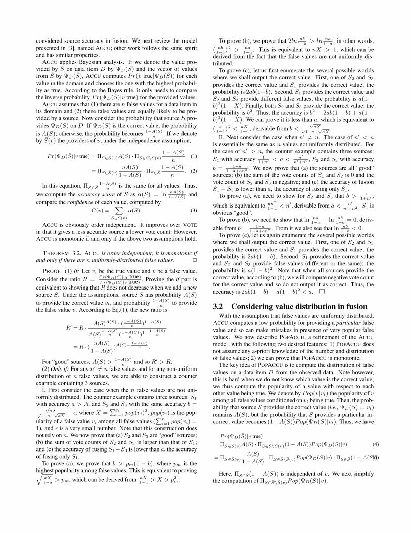
considered source accuracy in fusion. We next review the modelpresented in [3], named ACCU; other work follows the same spiritand has similar properties.
ACCU applies Bayesian analysis. If we denote the value pro-vided by S on data item D by ΨD(S) and the vector of valuesfrom S by ΨD(S), ACCU computes Pr(v true|ΨD(S)) for eachvalue in the domain and chooses the one with the highest probabil-ity as true. According to the Bayes rule, it only needs to comparethe inverse probability Pr(ΨD(S)|v true) for the provided values.
ACCU assumes that (1) there are n false values for a data item inits domain and (2) these false values are equally likely to be pro-vided by a source. Now consider the probability that source S pro-vides ΨD(S) on D. If ΨD(S) is the correct value, the probabilityis A(S); otherwise, the probability becomes 1−A(S)
n. If we denote
by S(v) the providers of v, under the independence assumption,
Pr(ΨD(S)|v true) = ΠS∈S(v)A(S) ·ΠS∈S\S(v)
1−A(S)
n(1)
= ΠS∈S(v)
nA(S)
1−A(S)·ΠS∈S
1−A(S)
n. (2)
In this equation, ΠS∈S1−A(S)
nis the same for all values. Thus,
we compute the accuracy score of S as α(S) = ln nA(S)1−A(S)
andcompare the confidence of each value, computed by
C(v) =X
S∈S(v)
α(S). (3)
ACCU is obviously order independent. It improves over VOTEin that it gives a less accurate source a lower vote count. However,ACCU is monotonic if and only if the above two assumptions hold.
THEOREM 3.2. ACCU is order independent; it is monotonic ifand only if there are n uniformly-distributed false values. 2
PROOF. (1) If: Let vt be the true value and v be a false value.Consider the ratio R = Pr(ΨD(S)|vt true)
Pr(ΨD(S)|v true). Proving the if part is
equivalent to showing that R does not decrease when we add a newsource S. Under the assumptions, source S has probability A(S)
to provide the correct value vt, and probability 1−A(S)n
to providethe false value v. According to Eq.(1), the new ratio is
R′ = R ·A(S)A(S) · ( 1−A(S)
n)1−A(S)
A(S)1−A(S)
n (1−A(S)
n)1−
1−A(S)n
= R · (nA(S)
1−A(S))A(S)− 1−A(S)
n .
For “good” sources, A(S) > 1−A(S)n
and so R′ > R.(2) Only if: For any n′ 6= n false values and for any non-uniform
distribution of n false values, we are able to construct a counterexample containing 3 sources.
I. First consider the case when the n false values are not uni-formly distributed. The counter example contains three sources: S1
with accuracy a > .5, and S2 and S3 with the same accuracy b =√aX√
1−a+√
aX− ε, where X =
Pni=1 pop(vi)
2, pop(vi) is the pop-ularity of a false value vi among all false values (
Pni=1 pop(vi) =
1), and ε is a very small number. Note that this construction doesnot rely on n. We now prove that (a) S2 and S3 are “good” sources;(b) the sum of vote counts of S2 and S3 is larger than that of S1;and (c) the accuracy of fusing S1−S3 is lower than a, the accuracyof fusing only S1.
To prove (a), we prove that b > pm(1 − b), where pm is thehighest popularity among false values. This is equivalent to provingq
aX1−a
> pm, which can be derived from aX1−a
> X > p2m.
To prove (b), we prove that 2ln nb1−b
> ln na1−a
; in other words,( nb1−b
)2 > na1−a
. This is equivalent to nX > 1, which can bederived from the fact that the false values are not uniformly dis-tributed.
To prove (c), let us first enumerate the several possible worldswhere we shall output the correct value. First, one of S2 and S3
provides the correct value and S1 provides the correct value; theprobability is 2ab(1−b). Second, S1 provides the correct value andS2 and S3 provide different false values; the probability is a(1 −b)2(1−X). Finally, both S2 and S3 provide the correct value; theprobability is b2. Thus, the accuracy is b2 + 2ab(1 − b) + a(1 −b)2(1 − X). We can prove it is less than a, which is equivalent to( b1−b
)2 < aX1−a
, derivable from b <√
aX√1−a+
√aX
.II. Next consider the case when n′ 6= n. The case of n′ < n
is essentially the same as n values not uniformly distributed. Forthe case of n′ > n, the counter example contains three sources:S1 with accuracy 1
1+n′ < a < n′
n′+n2 , S2 and S3 with accuracyb = 1−a
1−a+an2 . We now prove that (a) the sources are all “good”sources; (b) the sum of the vote counts of S1 and S2 is 0 and thevote count of S2 and S3 is negative; and (c) the accuracy of fusionS1 − S3 is lower than a, the accuracy of fusing only S1.
To prove (a), we need to show for S2 and S3 that b > 11+n′ ,
which is equivalent to an2
1−a< n′, derivable from a < n′
n′+n2 . S1 isobvious “good”.
To prove (b), we need to show that ln na1−a
+ ln nb1−b
= 0, deriv-able from b = 1−a
1−a+an2 . From it we also see that ln nb1−b
< 0.To prove (c), let us again enumerate the several possible worlds
where we shall output the correct value. First, one of S2 and S3
provides the correct value and S1 provides the correct value; theprobability is 2ab(1 − b). Second, S1 provides the correct valueand S2 and S3 provide false values (different or the same); theprobability is a(1 − b)2. Note that when all sources provide thecorrect value, according to (b), we will compute negative vote countfor the correct value and so do not output it as correct. Thus, theaccuracy is 2ab(1− b) + a(1− b)2 < a.
3.2 Considering value distribution in fusionWith the assumption that false values are uniformly distributed,
ACCU computes a low probability for providing a particular falsevalue and so can make mistakes in presence of very popular falsevalues. We now describe POPACCU, a refinement of the ACCUmodel, with the following two desired features: 1) POPACCU doesnot assume any a-priori knowledge of the number and distributionof false values; 2) we can prove that POPACCU is monotonic.
The key idea of POPACCU is to compute the distribution of falsevalues on a data item D from the observed data. Note however,this is hard when we do not know which value is the correct value;we thus compute the popularity of a value with respect to eachother value being true. We denote by Pop(v|vt) the popularity of vamong all false values conditioned on vt being true. Then, the prob-ability that source S provides the correct value (i.e., ΨD(S) = vt)remains A(S), but the probability that S provides a particular in-correct value becomes (1−A(S))Pop(ΨD(S)|vt). Thus, we have
Pr(ΨD(S)|v true)= ΠS∈S(v)A(S) ·ΠS∈S\S(v)(1−A(S))Pop(ΨD(S)|v) (4)
= ΠS∈S(v)
A(S)
1−A(S)·ΠS∈S\S(v)Pop(ΨD(S)|v) ·ΠS∈S(1−A(S)).(5)
Here, ΠS∈S(1 − A(S)) is independent of v. We next simplifythe computation of ΠS∈S\S(v)Pop(ΨD(S)|v).
0.7
0.75
0.8
0.85
0.9
0.95
1
0 5 10 15 20
Acc
ura
cy
#Sources
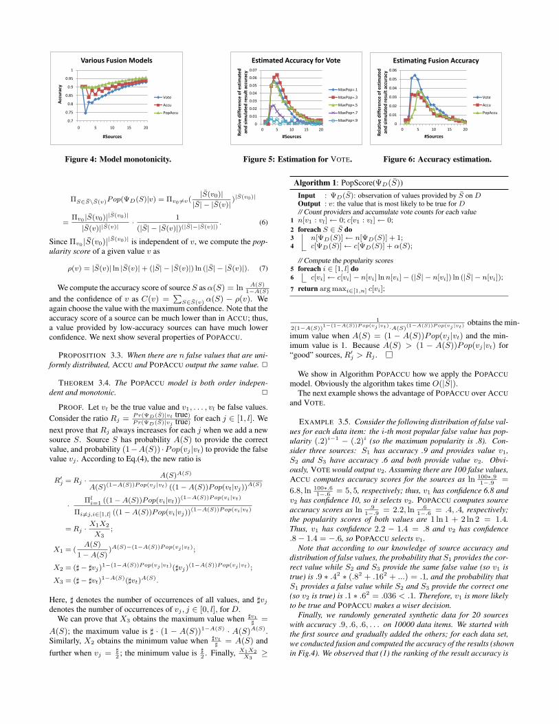
Various Fusion Models
Vote
Accu
PopAccu
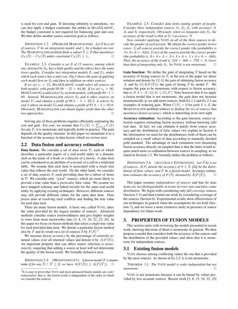
Figure 4: Model monotonicity.
0
0.01
0.02
0.03
0.04
0.05
0.06
0.07
0 5 10 15 20
Re
lati
ve d
iffe
ren
ce o
f e
stim
ate
d
and
sim
ula
ted
res
ult
acc
ura
cy
#Sources
Estimated Accuracy for Vote
MaxPop=.1
MaxPop=.3
MaxPop=.5
MaxPop=.7
MaxPop=.9
Figure 5: Estimation for VOTE.
0
0.01
0.02
0.03
0.04
0.05
0.06
0 5 10 15 20
Re
lati
ve d
iffe
ren
ce o
f es
tim
ated
an
d s
imu
late
d r
esu
lt a
ccu
racy
#Sources
Estimating Fusion Accuracy
Vote
Accu
PopAccu
Figure 6: Accuracy estimation.
ΠS∈S\S(v)Pop(ΨD(S)|v) = Πv0 6=v(|S(v0)||S| − |S(v)|
)|S(v0)|
=Πv0 |S(v0)||S(v0)|
|S(v)||S(v)|·
1
(|S| − |S(v)|)(|S|−|S(v)|). (6)
Since Πv0 |S(v0)||S(v0)| is independent of v, we compute the pop-ularity score of a given value v as
ρ(v) = |S(v)| ln |S(v)|+ (|S| − |S(v)|) ln (|S| − |S(v)|). (7)
We compute the accuracy score of source S as α(S) = ln A(S)1−A(S)
and the confidence of v as C(v) =P
S∈S(v) α(S) − ρ(v). Weagain choose the value with the maximum confidence. Note that theaccuracy score of a source can be much lower than in ACCU; thus,a value provided by low-accuracy sources can have much lowerconfidence. We next show several properties of POPACCU.
PROPOSITION 3.3. When there are n false values that are uni-formly distributed, ACCU and POPACCU output the same value. 2
THEOREM 3.4. The POPACCU model is both order indepen-dent and monotonic. 2
PROOF. Let vt be the true value and v1, . . . , vl be false values.Consider the ratio Rj = Pr(ΨD(S)|vt true)
Pr(ΨD(S)|vj true)for each j ∈ [1, l]. We
next prove that Rj always increases for each j when we add a newsource S. Source S has probability A(S) to provide the correctvalue, and probability (1−A(S)) ·Pop(vj |vt) to provide the falsevalue vj . According to Eq.(4), the new ratio is
R′j = Rj ·
A(S)A(S)
A(S)(1−A(S))Pop(vj |vt) ((1−A(S))Pop(vt|vj))A(S)
·Πl
i=1 ((1−A(S))Pop(vi|vt))(1−A(S))Pop(vi|vt)
Πi6=j,i∈[1,l] ((1−A(S))Pop(vi|vj))(1−A(S))Pop(vi|vt)
= Rj ·X1X2
X3;
X1 = (A(S)
1−A(S))A(S)−(1−A(S))Pop(vj |vt);
X2 = (]− ]vj)1−(1−A(S))Pop(vj |vt)(]vj)
(1−A(S))Pop(vj |vt);
X3 = (]− ]vt)1−A(S)(]vt)
A(S).
Here, ] denotes the number of occurrences of all values, and ]vj
denotes the number of occurrences of vj , j ∈ [0, l], for D.We can prove that X3 obtains the maximum value when ]vt
]=
A(S); the maximum value is ] · (1 − A(S))1−A(S) · A(S)A(S).Similarly, X2 obtains the minimum value when ]vt
]= A(S) and
further when vj = ]2
; the minimum value is ]2
. Finally, X1X2X3
≥
Algorithm 1: PopScore(ΨD(S))
Input : ΨD(S): observation of values provided by S on DOutput : v: the value that is most likely to be true for D// Count providers and accumulate vote counts for each valuen[v1 : vl]← 0; c[v1 : vl]← 0;1foreach S ∈ S do2
n[ΨD(S)]← n[ΨD(S)] + 1;3c[ΨD(S)]← c[ΨD(S)] + α(S);4
// Compute the popularity scoresforeach i ∈ [1, l] do5
c[vi]← c[vi]− n[vi] ln n[vi]− (|S| − n[vi]) ln (|S| − n[vi]);6
return arg maxi∈[1,n] c[vi];7
1
2(1−A(S))1−(1−A(S))P op(vj |vt)·A(S)
(1−A(S))P op(vj |vt)obtains the min-
imum value when A(S) = (1 − A(S))Pop(vj |vt) and the min-imum value is 1. Because A(S) > (1 − A(S))Pop(vj |vt) for“good” sources, R′
j > Rj .
We show in Algorithm POPACCU how we apply the POPACCUmodel. Obviously the algorithm takes time O(|S|).
The next example shows the advantage of POPACCU over ACCUand VOTE.
EXAMPLE 3.5. Consider the following distribution of false val-ues for each data item: the i-th most popular false value has pop-ularity (.2)i−1 − (.2)i (so the maximum popularity is .8). Con-sider three sources: S1 has accuracy .9 and provides value v1,S2 and S3 have accuracy .6 and both provide value v2. Obvi-ously, VOTE would output v2. Assuming there are 100 false values,ACCU computes accuracy scores for the sources as ln 100∗.9
1−.9=
6.8, ln 100∗.61−.6
= 5, 5, respectively; thus, v1 has confidence 6.8 andv2 has confidence 10, so it selects v2. POPACCU computes sourceaccuracy scores as ln .9
1−.9= 2.2, ln .6
1−.6= .4, .4, respectively;
the popularity scores of both values are 1 ln 1 + 2 ln 2 = 1.4.Thus, v1 has confidence 2.2 − 1.4 = .8 and v2 has confidence.8− 1.4 = −.6, so POPACCU selects v1.
Note that according to our knowledge of source accuracy anddistribution of false values, the probability that S1 provides the cor-rect value while S2 and S3 provide the same false value (so v1 istrue) is .9 ∗ .42 ∗ (.82 + .162 + ...) = .1, and the probability thatS1 provides a false value while S2 and S3 provide the correct one(so v2 is true) is .1 ∗ .62 = .036 < .1. Therefore, v1 is more likelyto be true and POPACCU makes a wiser decision.
Finally, we randomly generated synthetic data for 20 sourceswith accuracy .9, .6, .6, . . . on 10000 data items. We started withthe first source and gradually added the others; for each data set,we conducted fusion and computed the accuracy of the results (shownin Fig.4). We observed that (1) the ranking of the result accuracy is
always POPACCU, ACCU and VOTE; and (2) POPACCU is mono-tonic but ACCU and VOTE are not. 2
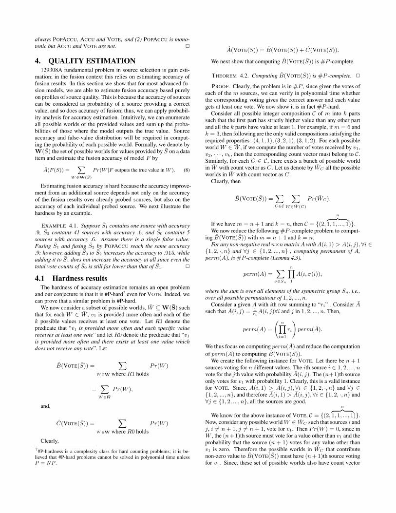
4. QUALITY ESTIMATION129308A fundamental problem in source selection is gain esti-
mation; in the fusion context this relies on estimating accuracy offusion results. In this section we show that for most advanced fu-sion models, we are able to estimate fusion accuracy based purelyon profiles of source quality. This is because the accuracy of sourcescan be considered as probability of a source providing a correctvalue, and so does accuracy of fusion; thus, we can apply probabil-ity analysis for accuracy estimation. Intuitively, we can enumerateall possible worlds of the provided values and sum up the proba-bilities of those where the model outputs the true value. Sourceaccuracy and false-value distribution will be required in comput-ing the probability of each possible world. Formally, we denote byW(S) the set of possible worlds for values provided by S on a dataitem and estimate the fusion accuracy of model F by
A(F (S)) =X
W∈W(S)
Pr(W |F outputs the true value in W ). (8)
Estimating fusion accuracy is hard because the accuracy improve-ment from an additional source depends not only on the accuracyof the fusion results over already probed sources, but also on theaccuracy of each individual probed source. We next illustrate thehardness by an example.
EXAMPLE 4.1. Suppose S1 contains one source with accuracy.9, S2 contains 41 sources with accuracy .6, and S0 contains 5sources with accuracy .6. Assume there is a single false value.Fusing S1 and fusing S2 by POPACCU reach the same accuracy.9; however, adding S0 to S2 increases the accuracy to .915, whileadding it to S1 does not increase the accuracy at all since even thetotal vote counts of S0 is still far lower than that of S1. 2
4.1 Hardness resultsThe hardness of accuracy estimation remains an open problem
and our conjecture is that it is #P-hard7 even for VOTE. Indeed, wecan prove that a similar problem is #P-hard.
We now consider a subset of possible worlds, W ⊆ W(S) suchthat for each W ∈ W , v1 is provided more often and each of thek possible values receives at least one vote. Let R1 denote thepredicate that “v1 is provided more often and each specific valuereceives at least one vote” and let R0 denote the predicate that “v1
is provided more often and there exists at least one value whichdoes not receive any vote”. Let
B(VOTE(S)) =X
W∈W where R1 holdsPr(W )
=X
W∈W
Pr(W ),
and,
C(VOTE(S)) =X
W∈W where R0 holdsPr(W )
Clearly,7#P-hardness is a complexity class for hard counting problems; it is be-lieved that #P-hard problems cannot be solved in polynomial time unlessP = NP .
A(VOTE(S)) = B(VOTE(S)) + C(VOTE(S)).
We next show that computing B(VOTE(S)) is #P -complete.
THEOREM 4.2. Computing B(VOTE(S)) is #P -complete. 2
PROOF. Clearly, the problem is in #P , since given the votes ofeach of the m sources, we can verify in polynomial time whetherthe corresponding voting gives the correct answer and each valuegets at least one vote. We now show it is in fact #P -hard.
Consider all possible integer composition C of m into k partssuch that the first part has strictly higher value than any other partand all the k parts have value at least 1. For example, if m = 6 andk = 3, then following are the only valid compositions satisfying therequired properties: (4, 1, 1), (3, 2, 1), (3, 1, 2). For each possibleworld W ∈ W , if we compute the number of votes received by v1,v2, · · · , vk, then the corresponding count vector must belong to C.Similarly, for each C ∈ C, there exists a bunch of possible worldin W with count vector as C. Let us denote by WC all the possibleworlds in W with count vector as C.
Clearly, then
B(VOTE(S)) =XC∈C
XW∈W (C)
Pr(WC).
If we have m = n + 1 and k = n, then C = {(2,
nz }| {1, 1, ..., 1)}.
We now reduce the following #P -complete problem to comput-ing B(VOTE(S)) with m = n + 1 and k = n:
For any non-negative real n×n matrix A with A(i, 1) > A(i, j), ∀i ∈{1, 2, ·, n} and ∀j ∈ {1, 2, ..., n} , computing permanent of A,perm(A), is #P -complete (Lemma 4.3).
perm(A) =X
σ∈Sn
nY1
A(i, σ(i)),
where the sum is over all elements of the symmetric group Sn, i.e.,over all possible permutations of 1, 2, ..., n.
Consider a given A with ith row summing to “ri” . Consider Asuch that A(i, j) = 1
riA(i, j)∀i and j in 1, 2, ..., n. Then,
perm(A) =
nY
i=1
ri
!perm(A).
We thus focus on computing perm(A) and reduce the computationof perm(A) to computing B(VOTE(S)).
We create the following instance for VOTE. Let there be n + 1sources voting for n different values. The ith source i ∈ 1, 2, ..., nvote for the jth value with probability A(i, j). The (n+1)th sourceonly votes for v1 with probability 1. Clearly, this is a valid instancefor VOTE. Since, A(i, 1) > A(i, j), ∀i ∈ {1, 2, ·, n} and ∀j ∈{1, 2, ..., n}, and therefore A(i, 1) > A(i, j), ∀i ∈ {1, 2, ·, n} and∀j ∈ {1, 2, ..., n}, all the sources are good.
We know for the above instance of VOTE, C = {(2,
nz }| {1, 1, ..., 1)}.
Now, consider any possible world W ∈ WC such that sources i andj, i 6= n + 1, j 6= n + 1, vote for v1. Then Pr(W ) = 0, since inW , the (n+1)th source must vote for a value other than v1 and theprobability that the source (n + 1) votes for any value other thanv1 is zero. Therefore the possible worlds in WC that contributenon-zero value to B(VOTE(S)) must have (n +1)th source votingfor v1. Since, these set of possible worlds also have count vector
{(2,
nz }| {1, 1, ..., 1)}, as a result, the voting function that denotes the
index of the value the first n sources vote for is a permutation.Hence,
B(VOTE(S)) = Pr(W ) = Pr(W ((2,
nz }| {1, 1, ..., 1)))
= Pr((n+1)th source votes for v1)X
σ∈Sn
nYi=1
Pr(source i votes for σ(i))
=X
σ∈Sn
nYi=1
Pr(source i votes for σ(i)) =X
σ∈Sn
nY1
A(i, σ(i)) = perm(A).
This completes the reduction and establishes the lemma.
In Lemma 4.3, we prove that computing permanent of any squarenon-negative real matrix with the first coordinate of each row hav-ing a value higher than the rest of the components is #P -complete.
LEMMA 4.3. For any non-negative real n × n matrix A withA(i, 1) > A(i, j), ∀i ∈ {1, 2, ·, n} and ∀j ∈ {1, 2, ..., n} , com-puting permanent of A, perm(A), is #P -complete.
perm(A) =X
σ∈Sn
nY1
A(i, σ(i)),
where the sum is over all elements of the symmetric group Sn, i.e.,over all possible permutations of 1, 2, ..., n.
PROOF. It is well-known due to a result of Valiant that comput-ing permanent of a 0 − 1 square matrix is #P -complete [19]. Wereduce the computation of permanent of any 0 − 1 square matrixto the permanent computation of the stated class of matrix in thislemma. Given any n×n 0−1 matrix B, we create a n+1×n+1matrix A by appending a column of length n + 1 with all en-tries equaling 2 and the (n+1)th row which has 2 in the first co-ordinate and zero elsewhere to B. That is, the first column of Ahas all entries equal to 2, A[2, 3, ..., n][2, 3, ..., n + 1] = B andA[n + 1][1, 2, ..., n + 1] = (2, 0, 0, ..., 0). It is easy to see thatperm(A) = 2perm(B). Therefore, if we can compute perm(A),then perm(B) can be computed as well.
We next describe a dynamic-programming algorithm that ap-proximates fusion accuracy in PTIME for VOTE and in pseudo-PTIME for other fusion models. Our approximation relies only onsource accuracy and the popularity of the most popular false value.
4.2 Accuracy estimation for VOTE
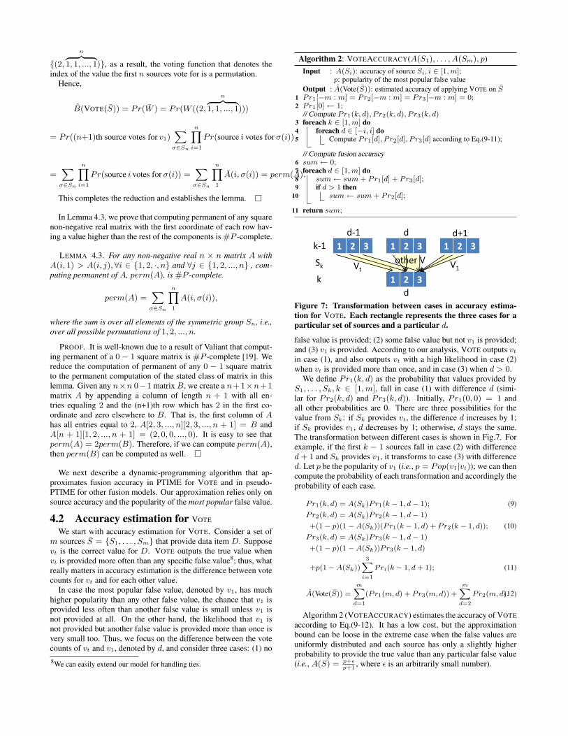
We start with accuracy estimation for VOTE. Consider a set ofm sources S = {S1, . . . , Sm} that provide data item D. Supposevt is the correct value for D. VOTE outputs the true value whenvt is provided more often than any specific false value8; thus, whatreally matters in accuracy estimation is the difference between votecounts for vt and for each other value.
In case the most popular false value, denoted by v1, has muchhigher popularity than any other false value, the chance that v1 isprovided less often than another false value is small unless v1 isnot provided at all. On the other hand, the likelihood that v1 isnot provided but another false value is provided more than once isvery small too. Thus, we focus on the difference between the votecounts of vt and v1, denoted by d, and consider three cases: (1) no8We can easily extend our model for handling ties.
Algorithm 2: VOTEACCURACY(A(S1), . . . , A(Sm), p)Input : A(Si): accuracy of source Si, i ∈ [1, m];
p: popularity of the most popular false valueOutput : A(Vote(S)): estimated accuracy of applying VOTE on SP r1[−m : m] = Pr2[−m : m] = Pr3[−m : m] = 0;1Pr1[0]← 1;2// Compute Pr1(k, d), P r2(k, d), P r3(k, d)foreach k ∈ [1, m] do3
foreach d ∈ [−i, i] do4Compute Pr1[d], P r2[d], P r3[d] according to Eq.(9-11);5
// Compute fusion accuracysum← 0;6foreach d ∈ [1, m] do7
sum← sum + Pr1[d] + Pr3[d];8if d > 1 then9
sum← sum + Pr2[d];10
return sum;11
1 2 3
1 2 3
Vt other V
1 2 3 1 2 3
V1
k-1
k
d-1 d d+1
d
Sk
Figure 7: Transformation between cases in accuracy estima-tion for VOTE. Each rectangle represents the three cases for aparticular set of sources and a particular d.
false value is provided; (2) some false value but not v1 is provided;and (3) v1 is provided. According to our analysis, VOTE outputs vt
in case (1), and also outputs vt with a high likelihood in case (2)when vt is provided more than once, and in case (3) when d > 0.
We define Pr1(k, d) as the probability that values provided byS1, . . . , Sk, k ∈ [1, m], fall in case (1) with difference d (simi-lar for Pr2(k, d) and Pr3(k, d)). Initially, Pr1(0, 0) = 1 andall other probabilities are 0. There are three possibilities for thevalue from Sk: if Sk provides vt, the difference d increases by 1;if Sk provides v1, d decreases by 1; otherwise, d stays the same.The transformation between different cases is shown in Fig.7. Forexample, if the first k − 1 sources fall in case (2) with differenced + 1 and Sk provides v1, it transforms to case (3) with differenced. Let p be the popularity of v1 (i.e., p = Pop(v1|vt)); we can thencompute the probability of each transformation and accordingly theprobability of each case.
Pr1(k, d) = A(Sk)Pr1(k − 1, d− 1); (9)Pr2(k, d) = A(Sk)Pr2(k − 1, d− 1)
+(1− p)(1−A(Sk))(Pr1(k − 1, d) + Pr2(k − 1, d)); (10)Pr3(k, d) = A(Sk)Pr3(k − 1, d− 1)
+(1− p)(1−A(Sk))Pr3(k − 1, d)
+p(1−A(Sk))3X
i=1
Pri(k − 1, d + 1); (11)
A(Vote(S)) =mX
d=1
(Pr1(m, d) + Pr3(m, d)) +mX
d=2
Pr2(m, d).(12)
Algorithm 2 (VOTEACCURACY) estimates the accuracy of VOTEaccording to Eq.(9-12). It has a low cost, but the approximationbound can be loose in the extreme case when the false values areuniformly distributed and each source has only a slightly higherprobability to provide the true value than any particular false value(i.e., A(S) = p+ε
p+1, where ε is an arbitrarily small number).
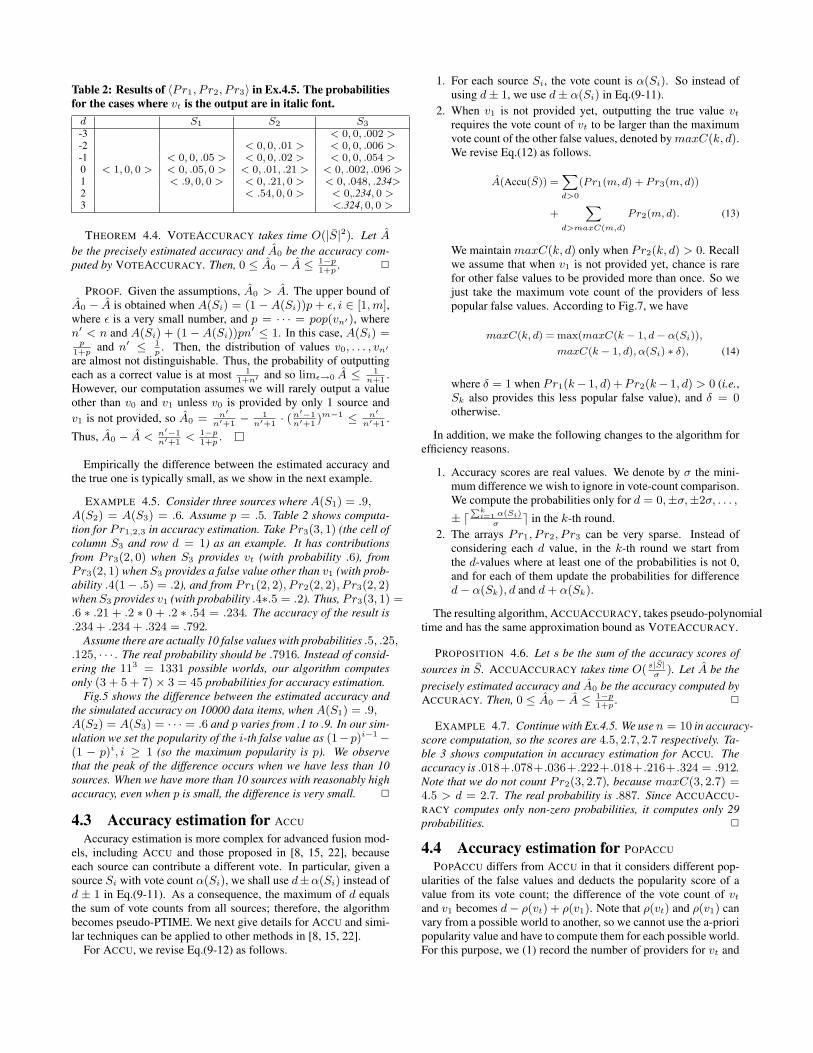
Table 2: Results of 〈Pr1, P r2, P r3〉 in Ex.4.5. The probabilitiesfor the cases where vt is the output are in italic font.
d S1 S2 S3
-3 < 0, 0, .002 >-2 < 0, 0, .01 > < 0, 0, .006 >-1 < 0, 0, .05 > < 0, 0, .02 > < 0, 0, .054 >0 < 1, 0, 0 > < 0, .05, 0 > < 0, .01, .21 > < 0, .002, .096 >1 < .9, 0, 0 > < 0, .21, 0 > < 0, .048, .234>2 < .54, 0, 0 > < 0,.234, 0 >3 <.324, 0, 0 >
THEOREM 4.4. VOTEACCURACY takes time O(|S|2). Let A
be the precisely estimated accuracy and A0 be the accuracy com-puted by VOTEACCURACY. Then, 0 ≤ A0 − A ≤ 1−p
1+p. 2
PROOF. Given the assumptions, A0 > A. The upper bound ofA0 − A is obtained when A(Si) = (1− A(Si))p + ε, i ∈ [1, m],where ε is a very small number, and p = · · · = pop(vn′), wheren′ < n and A(Si) + (1 − A(Si))pn′ ≤ 1. In this case, A(Si) =
p1+p
and n′ ≤ 1p
. Then, the distribution of values v0, . . . , vn′
are almost not distinguishable. Thus, the probability of outputtingeach as a correct value is at most 1
1+n′ and so limε→0 A ≤ 1n+1
.However, our computation assumes we will rarely output a valueother than v0 and v1 unless v0 is provided by only 1 source andv1 is not provided, so A0 = n′
n′+1− 1
n′+1· (n′−1
n′+1)m−1 ≤ n′
n′+1.
Thus, A0 − A < n′−1n′+1
< 1−p1+p
.
Empirically the difference between the estimated accuracy andthe true one is typically small, as we show in the next example.
EXAMPLE 4.5. Consider three sources where A(S1) = .9,A(S2) = A(S3) = .6. Assume p = .5. Table 2 shows computa-tion for Pr1,2,3 in accuracy estimation. Take Pr3(3, 1) (the cell ofcolumn S3 and row d = 1) as an example. It has contributionsfrom Pr3(2, 0) when S3 provides vt (with probability .6), fromPr3(2, 1) when S3 provides a false value other than v1 (with prob-ability .4(1− .5) = .2), and from Pr1(2, 2), P r2(2, 2), P r3(2, 2)when S3 provides v1 (with probability .4∗.5 = .2). Thus, Pr3(3, 1) =.6 ∗ .21 + .2 ∗ 0 + .2 ∗ .54 = .234. The accuracy of the result is.234 + .234 + .324 = .792.
Assume there are actually 10 false values with probabilities .5, .25,.125, · · · . The real probability should be .7916. Instead of consid-ering the 113 = 1331 possible worlds, our algorithm computesonly (3 + 5 + 7)× 3 = 45 probabilities for accuracy estimation.
Fig.5 shows the difference between the estimated accuracy andthe simulated accuracy on 10000 data items, when A(S1) = .9,A(S2) = A(S3) = · · · = .6 and p varies from .1 to .9. In our sim-ulation we set the popularity of the i-th false value as (1−p)i−1−(1 − p)i, i ≥ 1 (so the maximum popularity is p). We observethat the peak of the difference occurs when we have less than 10sources. When we have more than 10 sources with reasonably highaccuracy, even when p is small, the difference is very small. 2
4.3 Accuracy estimation for ACCU
Accuracy estimation is more complex for advanced fusion mod-els, including ACCU and those proposed in [8, 15, 22], becauseeach source can contribute a different vote. In particular, given asource Si with vote count α(Si), we shall use d±α(Si) instead ofd ± 1 in Eq.(9-11). As a consequence, the maximum of d equalsthe sum of vote counts from all sources; therefore, the algorithmbecomes pseudo-PTIME. We next give details for ACCU and simi-lar techniques can be applied to other methods in [8, 15, 22].
For ACCU, we revise Eq.(9-12) as follows.
1. For each source Si, the vote count is α(Si). So instead ofusing d± 1, we use d± α(Si) in Eq.(9-11).
2. When v1 is not provided yet, outputting the true value vt
requires the vote count of vt to be larger than the maximumvote count of the other false values, denoted by maxC(k, d).We revise Eq.(12) as follows.
A(Accu(S)) =Xd>0
(Pr1(m, d) + Pr3(m, d))
+X
d>maxC(m,d)
Pr2(m, d). (13)
We maintain maxC(k, d) only when Pr2(k, d) > 0. Recallwe assume that when v1 is not provided yet, chance is rarefor other false values to be provided more than once. So wejust take the maximum vote count of the providers of lesspopular false values. According to Fig.7, we have
maxC(k, d) = max(maxC(k − 1, d− α(Si)),
maxC(k − 1, d), α(Si) ∗ δ), (14)
where δ = 1 when Pr1(k− 1, d)+Pr2(k− 1, d) > 0 (i.e.,Sk also provides this less popular false value), and δ = 0otherwise.
In addition, we make the following changes to the algorithm forefficiency reasons.
1. Accuracy scores are real values. We denote by σ the mini-mum difference we wish to ignore in vote-count comparison.We compute the probabilities only for d = 0,±σ,±2σ, . . . ,
± dPk
i=1 α(Si)
σe in the k-th round.
2. The arrays Pr1, P r2, P r3 can be very sparse. Instead ofconsidering each d value, in the k-th round we start fromthe d-values where at least one of the probabilities is not 0,and for each of them update the probabilities for differenced− α(Sk), d and d + α(Sk).
The resulting algorithm, ACCUACCURACY, takes pseudo-polynomialtime and has the same approximation bound as VOTEACCURACY.
PROPOSITION 4.6. Let s be the sum of the accuracy scores ofsources in S. ACCUACCURACY takes time O( s|S|
σ). Let A be the
precisely estimated accuracy and A0 be the accuracy computed byACCURACY. Then, 0 ≤ A0 − A ≤ 1−p
1+p. 2
EXAMPLE 4.7. Continue with Ex.4.5. We use n = 10 in accuracy-score computation, so the scores are 4.5, 2.7, 2.7 respectively. Ta-ble 3 shows computation in accuracy estimation for ACCU. Theaccuracy is .018+.078+.036+.222+.018+.216+.324 = .912.Note that we do not count Pr2(3, 2.7), because maxC(3, 2.7) =4.5 > d = 2.7. The real probability is .887. Since ACCUACCU-RACY computes only non-zero probabilities, it computes only 29probabilities. 2
4.4 Accuracy estimation for POPACCU
POPACCU differs from ACCU in that it considers different pop-ularities of the false values and deducts the popularity score of avalue from its vote count; the difference of the vote count of vt
and v1 becomes d− ρ(vt) + ρ(v1). Note that ρ(vt) and ρ(v1) canvary from a possible world to another, so we cannot use the a-prioripopularity value and have to compute them for each possible world.For this purpose, we (1) record the number of providers for vt and
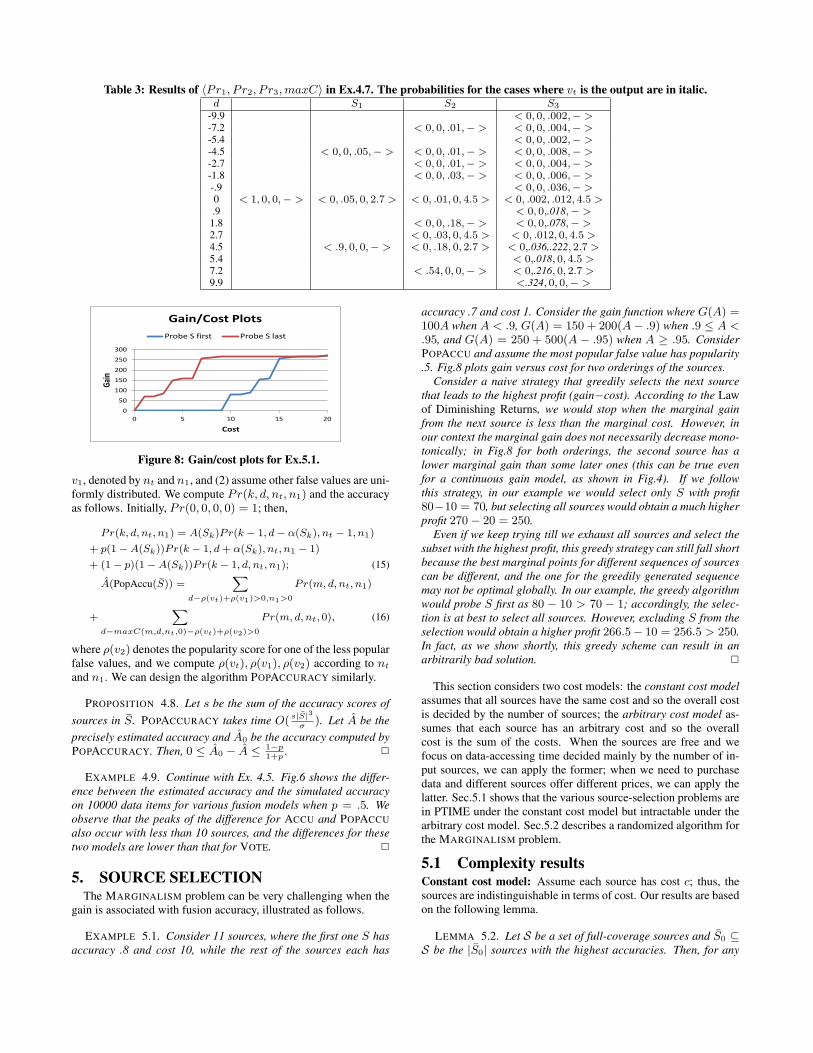
Table 3: Results of 〈Pr1, P r2, P r3, maxC〉 in Ex.4.7. The probabilities for the cases where vt is the output are in italic.d S1 S2 S3
-9.9 < 0, 0, .002,− >-7.2 < 0, 0, .01,− > < 0, 0, .004,− >-5.4 < 0, 0, .002,− >-4.5 < 0, 0, .05,− > < 0, 0, .01,− > < 0, 0, .008,− >-2.7 < 0, 0, .01,− > < 0, 0, .004,− >-1.8 < 0, 0, .03,− > < 0, 0, .006,− >-.9 < 0, 0, .036,− >0 < 1, 0, 0,− > < 0, .05, 0, 2.7 > < 0, .01, 0, 4.5 > < 0, .002, .012, 4.5 >.9 < 0, 0,.018,− >1.8 < 0, 0, .18,− > < 0, 0,.078,− >2.7 < 0, .03, 0, 4.5 > < 0, .012, 0, 4.5 >4.5 < .9, 0, 0,− > < 0, .18, 0, 2.7 > < 0,.036,.222, 2.7 >5.4 < 0,.018, 0, 4.5 >7.2 < .54, 0, 0,− > < 0,.216, 0, 2.7 >9.9 <.324, 0, 0,− >
0
50
100
150
200
250
300
0 5 10 15 20
Gain
Cost
Gain/Cost Plots
Probe S first Probe S last
Figure 8: Gain/cost plots for Ex.5.1.
v1, denoted by nt and n1, and (2) assume other false values are uni-formly distributed. We compute Pr(k, d, nt, n1) and the accuracyas follows. Initially, Pr(0, 0, 0, 0) = 1; then,
Pr(k, d, nt, n1) = A(Sk)Pr(k − 1, d− α(Sk), nt − 1, n1)
+ p(1−A(Sk))Pr(k − 1, d + α(Sk), nt, n1 − 1)
+ (1− p)(1−A(Sk))Pr(k − 1, d, nt, n1); (15)
A(PopAccu(S)) =X
d−ρ(vt)+ρ(v1)>0,n1>0
Pr(m, d, nt, n1)
+X
d−maxC(m,d,nt,0)−ρ(vt)+ρ(v2)>0
Pr(m, d, nt, 0), (16)
where ρ(v2) denotes the popularity score for one of the less popularfalse values, and we compute ρ(vt), ρ(v1), ρ(v2) according to nt
and n1. We can design the algorithm POPACCURACY similarly.
PROPOSITION 4.8. Let s be the sum of the accuracy scores ofsources in S. POPACCURACY takes time O( s|S|3
σ). Let A be the
precisely estimated accuracy and A0 be the accuracy computed byPOPACCURACY. Then, 0 ≤ A0 − A ≤ 1−p
1+p. 2
EXAMPLE 4.9. Continue with Ex. 4.5. Fig.6 shows the differ-ence between the estimated accuracy and the simulated accuracyon 10000 data items for various fusion models when p = .5. Weobserve that the peaks of the difference for ACCU and POPACCUalso occur with less than 10 sources, and the differences for thesetwo models are lower than that for VOTE. 2
5. SOURCE SELECTIONThe MARGINALISM problem can be very challenging when the
gain is associated with fusion accuracy, illustrated as follows.
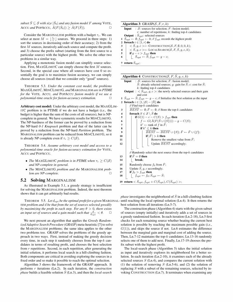
EXAMPLE 5.1. Consider 11 sources, where the first one S hasaccuracy .8 and cost 10, while the rest of the sources each has
accuracy .7 and cost 1. Consider the gain function where G(A) =100A when A < .9, G(A) = 150 + 200(A− .9) when .9 ≤ A <.95, and G(A) = 250 + 500(A − .95) when A ≥ .95. ConsiderPOPACCU and assume the most popular false value has popularity.5. Fig.8 plots gain versus cost for two orderings of the sources.
Consider a naive strategy that greedily selects the next sourcethat leads to the highest profit (gain−cost). According to the Lawof Diminishing Returns, we would stop when the marginal gainfrom the next source is less than the marginal cost. However, inour context the marginal gain does not necessarily decrease mono-tonically; in Fig.8 for both orderings, the second source has alower marginal gain than some later ones (this can be true evenfor a continuous gain model, as shown in Fig.4). If we followthis strategy, in our example we would select only S with profit80−10 = 70, but selecting all sources would obtain a much higherprofit 270− 20 = 250.
Even if we keep trying till we exhaust all sources and select thesubset with the highest profit, this greedy strategy can still fall shortbecause the best marginal points for different sequences of sourcescan be different, and the one for the greedily generated sequencemay not be optimal globally. In our example, the greedy algorithmwould probe S first as 80 − 10 > 70 − 1; accordingly, the selec-tion is at best to select all sources. However, excluding S from theselection would obtain a higher profit 266.5− 10 = 256.5 > 250.In fact, as we show shortly, this greedy scheme can result in anarbitrarily bad solution. 2
This section considers two cost models: the constant cost modelassumes that all sources have the same cost and so the overall costis decided by the number of sources; the arbitrary cost model as-sumes that each source has an arbitrary cost and so the overallcost is the sum of the costs. When the sources are free and wefocus on data-accessing time decided mainly by the number of in-put sources, we can apply the former; when we need to purchasedata and different sources offer different prices, we can apply thelatter. Sec.5.1 shows that the various source-selection problems arein PTIME under the constant cost model but intractable under thearbitrary cost model. Sec.5.2 describes a randomized algorithm forthe MARGINALISM problem.
5.1 Complexity resultsConstant cost model: Assume each source has cost c; thus, thesources are indistinguishable in terms of cost. Our results are basedon the following lemma.
LEMMA 5.2. Let S be a set of full-coverage sources and S0 ⊆S be the |S0| sources with the highest accuracies. Then, for any
subset S ⊆ S with size |S0| and any fusion model F among VOTE,ACCU and POPACCU, A(F (S0)) ≥ A(F (S)). 2
Consider the MARGINALISM problem with a budget τc. We canselect at most M = b τc
cc sources. We proceed in three steps: 1)
sort the sources in decreasing order of their accuracy; 2) from thefirst M sources, iteratively add each source and compute the profit.and 3) choose the prefix subset (starting from the first source to aparticular source) with the highest profit. We solve the other twoproblems in a similar way.
Applying a monotonic fusion model can simplify source selec-tion. First, MAXGLIMITC can simply choose the first M sources.Second, in the special case where all sources have cost 0 so es-sentially the goal is to maximize fusion accuracy, we can simplychoose all sources (recall that we consider only “good” sources).
THEOREM 5.3. Under the constant cost model, the problemsMAXGLIMITC, MINCLIMITG, and MARGINALISM are in PTIMEfor the VOTE, ACCU, and POPACCU fusion models if we use apolynomial-time oracle for fusion-accuracy estimation. 2
Arbitrary cost model: Under the arbitrary cost model, the MAXGLIM-ITC problem is in PTIME if we do not have a budget (i.e., thebudget is higher than the sum of the costs of all sources), but is NP-complete in general. We have symmetric results for MINCLIMITG.The NP-hardness of the former can be proved by a reduction fromthe NP-hard 0-1 Knapsack problem and that of the latter can beproved by a reduction from the NP-hard Partition problem. TheMARGINALISM problem can be reduced from MINCLIMITG, so itis already NP complete even if τc ≥ C(S).
THEOREM 5.4. Assume arbitrary cost model and access to apolynomial-time oracle for fusion-accuracy estimation for VOTE,ACCU and POPACCU.
• The MAXGLIMITC problem is in PTIME when τc ≥ C(S)and NP-complete in general.
• The MINCLIMITG problem and the MARGINALISM prob-lem are NP-complete. 2
5.2 Solving MARGINALISMAs illustrated in Example 5.1, a greedy strategy is insufficient
for solving the MARGINALISM problem. Indeed, the next theoremshows that it can get arbitrarily bad results.
THEOREM 5.5. Let dopt be the optimal profit for a given MARGINAL-ISM problem and d be that from the set of sources selected greedilyby maximizing the profit in each step. For any θ > 0, there existsan input set of sources and a gain model such that d
dopt< θ. 2
We next present an algorithm that applies the Greedy Random-ized Adaptive Search Procedure (GRASP) meta-heuristic [7] to solvethe MARGINALISM problems; the same idea applies to the othertwo problems too. GRASP solves the problems of the greedy ap-proach in two ways. First, instead of making the greedy decisionevery time, in each step it randomly chooses from the top-k can-didates in terms of resulting profit, and chooses the best selectionfrom r repetitions. Second, in each repetition, after generating theinitial solution, it performs local search in a hill-climbing fashion.Both components are critical in avoiding exploring the sources in afixed order and so make it possible to reach the optimal selection.
Algorithm 3 shows the framework of the GRASP approach. Itperforms r iterations (Ln.2). In each iteration, the constructionphase builds a feasible solution S (Ln.3), and then the local-search
Algorithm 3: GRASP(S, F, r, k)Input : S: sources for selection; F : fusion model;
r: number of repetitions; k: finding top-k candidatesOutput : Sopt: selected sourcesSopt ← ∅; fopt ← 0; // fopt records the highest profit1foreach i ∈ [1, r] do2
< S, g, c >← CONSTRUCTION(S, F, ∅, 0, 0, k);3< S, g, c >← LOCALSEARCH(S, F, S, g, c, k);4if g − c > fopt then5
Sopt ← S; fopt ← g − c;6
return Sopt;7
Algorithm 4: CONSTRUCTION(S, F, S, g, c, k)Input : S: sources for selection; F : fusion model;
S: already selected sources; g: gain for S; c: cost for S;k: finding top-k candidates
Output : < Sopt, g, c >: the newly selected sources and their gainand cost
Sopt ← S; fopt ← g − c; // Initialize the best solution as the input1foreach i ∈ [1, |S| − |S|] do2
// Find top-k candidatesBEST ← ∅; F ← ∅; // Store the top-k candidates3foreach S ∈ S \ S do4
if G(1)− c− C(S) > fopt then5f ← G(A(F (S ∪ {S})))− g − C(S);6k′ ← rank of f in F ;7if k′ ≤ k then8
BEST ← BEST ∪ {S}; F ← F ∪ {f};9if |F | > k then10
Remove the smallest value from F ;11Update BEST accordingly;12
// Randomly select the next source from the top-k candidatesif F = ∅ then13
break;14
Randomly choose f0 from F ;15Update S, g, c accordingly;16if f0 > fopt then17
fopt ← f0; Sopt ← S;18
return < Sopt, fopt + C(Sopt), C(Sopt) >;19
phase investigates the neighborhood of S in a hill-climbing fashionuntil reaching the local optimal solution (Ln.4). It then returns thebest solution from all iterations (Ln.5-7).
The construction phase (Algorithm 4) starts with the given subsetof sources (empty initially) and iteratively adds a set of sources ina greedy randomized fashion. In each iteration (Ln.2-18), Ln.5 firstchecks for each remaining source whether beating the current bestsolution is possible by reaching the maximum possible gain (i.e.,G(1)), and skips the source if not. Ln.6 estimates the differencebetween the marginal gain and marginal cost of adding the source.Then, Ln.7-12 maintains the top-k candidates; Ln.13-16 randomlyselects one of them to add next. Finally, Ln.17-19 chooses the pre-fix subset with the highest profit.
The local-search phase (Algorithm 5) takes the initial solutionas input and iteratively explores its neighborhood for a better so-lution. In each iteration (Ln.2-10), it examines each of the alreadyselected sources S (Ln.4), and compares the current solution with(1) the solution of removing S (Ln.5-6), and (2) the solution ofreplacing S with a subset of the remaining sources, selected by in-voking CONSTRUCTION (Ln.7). It terminates when examining any
Algorithm 5: LOCALSEARCH(S, F, S, g, c, k)Input : S: sources for selection; F : fusion model;
S: already selected sources; g: gain for S; c: cost for S;k: finding top-k candidates
Output : < Sopt, g, c >: the newly selected sources and their gainand cost
changed← true;1while changed do2
changed← false;3foreach S ∈ S do4
S0 ← S \ {S}; c0 ← c− C(S);5g0 ← G(A(F (S0)));// Invoke estimation methods6< S0, g0, c0 >←CONSTRUCTION(S, F, S0, g0, c0, k);7if g0 − c0 > g − c then8
S ← S0; g = g0; c = c0;9changed← true; break;10
return < S, g, c >;11
selected source cannot improve the solution (Ln.2, Ln.8-10). Sincethe profit cannot grow infinitely, the local search will converge.
Note that when k = 1, all iterations of GRASP will generatethe same result and the algorithm regresses to a hill-climbing algo-rithm. When k = |S|, the construction phase can generate anyordering of the sources and a high r leads to an algorithm thatessentially enumerates all possible source orderings. Our experi-ments show that with a continuous gain model, setting k = 5 andr = 20 can obtain the optimal solution most of the time for morethan 200 sources, but with a non-continuous gain model, we needto set much higher k and r.
EXAMPLE 5.6. Consider 8 sources: the first, S, has accuracy.8 and cost 5; and each of the rest has accuracy .7 and cost 1.Consider POPACCU and gain function G(A) = 100A. Assumek = 1, so the algorithm regresses to a hill-climbing algorithm.
The construction phase first selects S as its profit is higher thanthe others (80 − 5 > 70 − 1). It then selects 5 other sources,reaching a profit of 96.2 − 10 = 86.2. The local-search phaseexamines S and finds that (1) removing S obtains a profit of 93.2−5 = 88.2; and (2) replacing S with the 2 remaining sources obtainsa profit of 96.2 − 7 = 89.2. Thus, it selects the 7 less accuratesources. It cannot further improve this solution and terminates. 2
6. EXTENSION FOR PARTIAL COVERAGEWe next extend our results for sources without full coverage. We
define the coverage of source S as the percentage of its provideddata items over D, denoted by V (S). First, considering coveragewould affect accuracy estimation. We need to revise Eq.(9-11) byconsidering the possibility that the k-th source does not provide thedata item at all.
Pr1(k, d) = V (Sk)A(Sk)Pr1(k − 1, d− 1); (17)Pr2(k, d) = V (Sk)A(Sk)Pr2(k − 1, d− 1)
+(1− V (Sk) + V (Sk)(1− p)(1−A(Sk)))
·(Pr1(k − 1, d) + Pr2(k − 1, d)); (18)Pr3(k, d) = V (Sk)A(Sk)Pr3(k − 1, d− 1)
+(1− V (Sk) + V (Sk)(1− p)(1−A(Sk)))Pr3(k − 1, d)
+V (Sk)p(1−A(Sk))3X
i=1
Pri(k − 1, d + 1); (19)
Note that the revised estimation already incorporates coverage ofthe results and is essentially the percentage of correctly provided
values over all data items (i.e., the product of coverage and accu-racy); we call it recall.
Second, the gain model can be revised to a function of recall suchthat it takes both coverage and accuracy into account. Lemma 5.2does not necessarily hold any more so whether the optimizationproblems are in PTIME under the constant cost model remains anopen problem. However, the GRASP algorithm still applies and wereport experimental results in Sec.7.
7. EXPERIMENTAL RESULTSThis section reports experimental results showing that (1) our
algorithms can select a subset of sources that maximizes fusion ac-curacy; (2) when we consider cost, we are able to efficiently finda subset of sources that together obtains nearly the highest profit;(3) POPACCU outperforms the other fusion models and we estimatefusion accuracy quite accurately; (4) our algorithms are scalable.
7.1 Experiments on real data
7.1.1 Experiment setupData: We experimented on two data sets. The Book data set con-tains 894 data sources that were registered at AbeBooks.com andprovided information on computer science books in 2007 (see Ex.1.1-1.2). In total they provided 24364 listings for 1265 books on ISBN,name, and authors; each source provides .1% to 86% of the books.By default, we set the coverage and accuracy of the sources ac-cording to a gold standard containing the author lists from the bookcover on 100 randomly selected books. In accuracy estimation weset the maximum popularity p as the largest popularity of false val-ues among all data items.
The Flight data set contains 38 Deep Web sources among top-200 results by Google for keyword search “flight status”. We col-lected data on 1200 flights for their flight number (serving as identi-fier), scheduled/actual departure/arrival time, and departure/arrivalgate on 12/8/2011 (see [10] for details of data collection). In totalthey provided 27469 records; each sources provides 1.6% to 100%of the flights. We used a gold standard containing data providedby the airline websites AA, UA, and Continental on 100 randomlyselected flights. We sampled source quality both for overall dataand for each attribute.
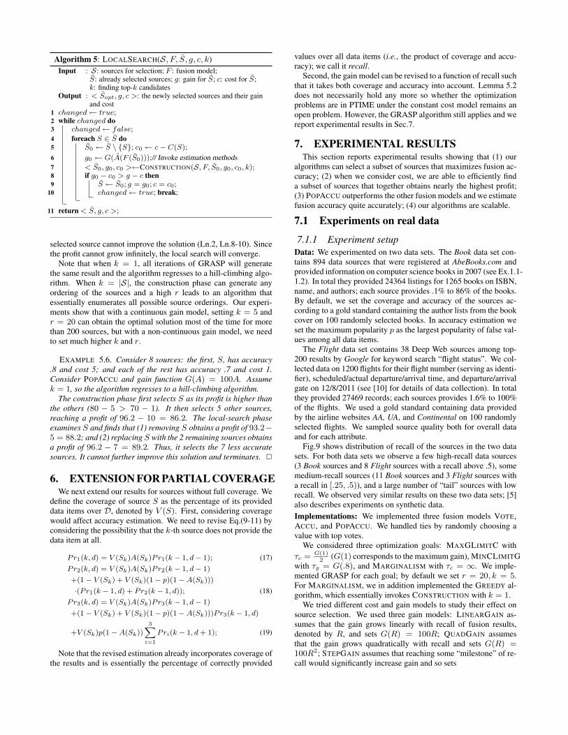
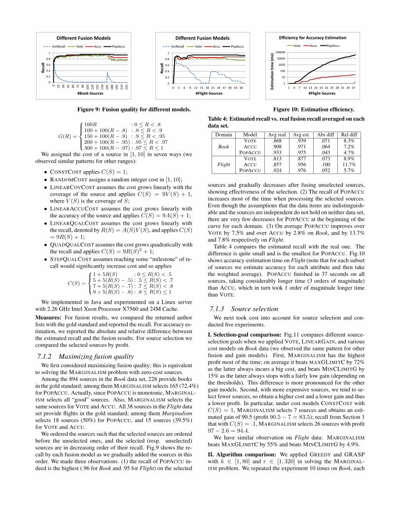
Fig.9 shows distribution of recall of the sources in the two datasets. For both data sets we observe a few high-recall data sources(3 Book sources and 8 Flight sources with a recall above .5), somemedium-recall sources (11 Book sources and 3 Flight sources witha recall in [.25, .5)), and a large number of “tail” sources with lowrecall. We observed very similar results on these two data sets; [5]also describes experiments on synthetic data.Implementations: We implemented three fusion models VOTE,ACCU, and POPACCU. We handled ties by randomly choosing avalue with top votes.
We considered three optimization goals: MAXGLIMITC withτc = G(1)
2(G(1) corresponds to the maximum gain), MINCLIMITG
with τg = G(.8), and MARGINALISM with τc = ∞. We imple-mented GRASP for each goal; by default we set r = 20, k = 5.For MARGINALISM, we in addition implemented the GREEDY al-gorithm, which essentially invokes CONSTRUCTION with k = 1.
We tried different cost and gain models to study their effect onsource selection. We used three gain models: LINEARGAIN as-sumes that the gain grows linearly with recall of fusion results,denoted by R, and sets G(R) = 100R; QUADGAIN assumesthat the gain grows quadratically with recall and sets G(R) =100R2; STEPGAIN assumes that reaching some “milestone” of re-call would significantly increase gain and so sets
0
0.2
0.4
0.6
0.8
1 0
15
30
45
60
75
90
10
5
12
0
13
5
15
0
16
5
18
0
19
5
21
0
22
5
Re
call
#Book-Sources
Different Fusion Models
SrcRecall Vote Accu PopAccu
0
0.2
0.4
0.6
0.8
1
0 3 6 9 12 15 18 21 24 27 30 33 36
Re
call
#Flight-Sources
Different Fusion Models
SrcRecall Vote Accu PopAccu
Figure 9: Fusion quality for different models.
1
10
100
1000
10000
100000
1 4 7 10 13 16 19 22 25 28 31 34 37 Esti
mat
ion
tim
e (m
s)
#Flight-Sources
Efficiency for Accuracy Estimation
Vote Accu PopAccu
Figure 10: Estimation efficiency.
G(R) =
8>>><>>>:100R : 0 ≤ R < .8100 + 100(R− .8) : .8 ≤ R < .9150 + 100(R− .9) : .9 ≤ R < .95200 + 100(R− .95) : .95 ≤ R < .97300 + 100(R− .97) : .97 ≤ R ≤ 1
We assigned the cost of a source in [1, 10] in seven ways (weobserved similar patterns for other ranges):
• CONSTCOST applies C(S) = 1;• RANDOMCOST assigns a random integer cost in [1, 10];• LINEARCOVCOST assumes the cost grows linearly with the
coverage of the source and applies C(S) = 9V (S) + 1,where V (S) is the coverage of S;
• LINEARACCUCOST assumes the cost grows linearly withthe accuracy of the source and applies C(S) = 9A(S) + 1;
• LINEARQUALCOST assumes the cost grows linearly withthe recall, denoted by R(S) = A(S)V (S), and applies C(S)= 9R(S) + 1;
• QUADQUALCOST assumes the cost grows quadratically withthe recall and applies C(S) = 9R(S)2 + 1;
• STEPQUALCOST assumes reaching some “milestone” of re-call would significantly increase cost and so applies
C(S) =
8><>:1 + 5R(S) : 0 ≤ R(S) < .55 + 5(R(S)− .5) : .5 ≤ R(S) < .77 + 5(R(S)− .7) : .7 ≤ R(S) < .89 + 5(R(S)− .8) : .8 ≤ R(S) ≤ 1
We implemented in Java and experimented on a Linux serverwith 2.26 GHz Intel Xeon Processor X7560 and 24M Cache.Measures: For fusion results, we compared the returned authorlists with the gold standard and reported the recall. For accuracy es-timation, we reported the absolute and relative difference betweenthe estimated recall and the fusion results. For source selection wecompared the selected sources by profit.
7.1.2 Maximizing fusion qualityWe first considered maximizing fusion quality; this is equivalent
to solving the MARGINALISM problem with zero-cost sources.Among the 894 sources in the Book data set, 228 provide books
in the gold standard; among them MARGINALISM selects 165 (72.4%)for POPACCU. Actually, since POPACCU is monotonic, MARGINAL-ISM selects all “good” sources. Also, MARGINALISM selects thesame sources for VOTE and ACCU. All 38 sources in the Flight dataset provide flights in the gold standard; among them Marginalismselects 18 sources (50%) for POPACCU, and 15 sources (39.5%)for VOTE and ACCU.
We ordered the sources such that the selected sources are orderedbefore the unselected ones, and the selected (resp. unselected)sources are in decreasing order of their recall. Fig.9 shows the re-call by each fusion model as we gradually added the sources in thisorder. We made three observations. (1) the recall of POPACCU in-deed is the highest (.96 for Book and .95 for Flight) on the selected
Table 4: Estimated recall vs. real fusion recall averaged on eachdata set.
Domain Model Avg real Avg est. Abs diff Rel diffVOTE .868 .939 .071 8.3%
Book ACCU .908 .971 .064 7.2%POPACCU .933 .975 .043 4.7%
VOTE .813 .877 .073 8.9%Flight ACCU .857 .956 .100 11.7%
POPACCU .924 .976 .052 5.7%
sources and gradually decreases after fusing unselected sources,showing effectiveness of the selection. (2) The recall of POPACCUincreases most of the time when processing the selected sources.Even though the assumptions that the data items are indistinguish-able and the sources are independent do not hold on neither data set,there are very few decreases for POPACCU at the beginning of thecurve for each domain. (3) On average POPACCU improves overVOTE by 7.5% and over ACCU by 2.8% on Book, and by 13.7%and 7.8% respectively on Flight.
Table 4 compares the estimated recall with the real one. Thedifference is quite small and is the smallest for POPACCU. Fig.10shows accuracy-estimation time on Flight (note that for each subsetof sources we estimate accuracy for each attribute and then takethe weighted average). POPACCU finished in 37 seconds on allsources, taking considerably longer time (3 orders of magnitude)than ACCU, which in turn took 1 order of magnitude longer timethan VOTE.
7.1.3 Source selectionWe next took cost into account for source selection and con-
ducted five experiments.
I. Selection-goal comparison: Fig.11 compares different source-selection goals when we applied VOTE, LINEARGAIN, and variouscost models on Book data (we observed the same pattern for otherfusion and gain models). First, MARGINALISM has the highestprofit most of the time; on average it beats MAXGLIMITC by 72%as the latter always incurs a big cost, and beats MINCLIMITG by15% as the latter always stops with a fairly low gain (depending onthe thresholds). This difference is more pronounced for the othergain models. Second, with more expensive sources, we tend to se-lect fewer sources, so obtain a higher cost and a lower gain and thusa lower profit. In particular, under cost models CONSTCOST withC(S) = 1, MARGINALISM selects 7 sources and obtains an esti-mated gain of 90.5 (profit 90.5− 7 = 83.5); recall from Section 1that with C(S) = .1, MARGINALISM selects 26 sources with profit97− 2.6 = 94.4.
We have similar observation on Flight data: MARGINALISMbeats MAXGLIMITC by 55% and beats MINCLIMITG by 4.9%.
II. Algorithm comparison: We applied GREEDY and GRASPwith k ∈ [1, 80] and r ∈ [1, 320] in solving the MARGINAL-ISM problem. We repeated the experiment 10 times on Book, each
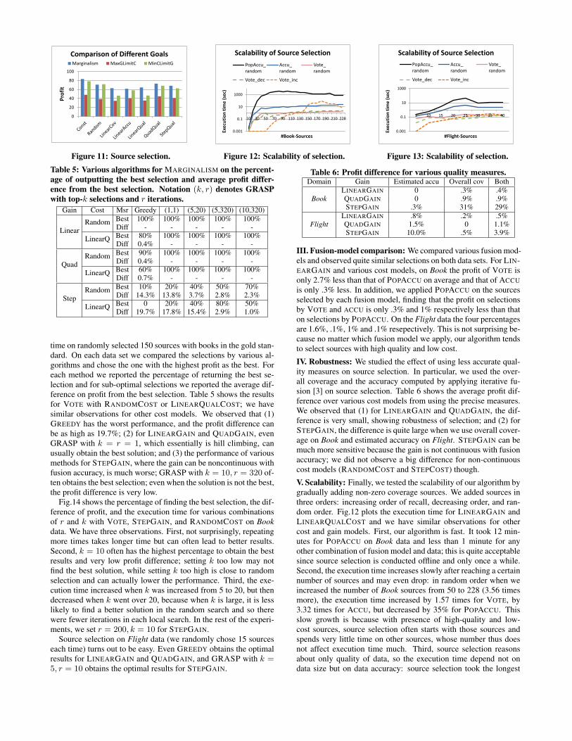
0
20
40
60
80
100
Pro
fit
Comparison of Different Goals Marginalism MaxGLimitC MinCLimitG
Figure 11: Source selection.
0.001
0.1
10
1000
10 30 50 70 90 110 130 150 170 190 210 228
Exec
uti
on
tim
e (s
ec)
#Book-Sources
Scalability of Source Selection
PopAccu_ random
Accu_ random
Vote_ random
Vote_dec Vote_inc
Figure 12: Scalability of selection.
0.001
0.1
10
1000
5 10 15 20 25 30 35 40
Exec
uti
on
tim
e (s
ec)
#Flight-Sources
Scalability of Source Selection
PopAccu_ random
Accu_ random
Vote_ random
Vote_dec Vote_inc
Figure 13: Scalability of selection.Table 5: Various algorithms for MARGINALISM on the percent-age of outputting the best selection and average profit differ-ence from the best selection. Notation (k, r) denotes GRASPwith top-k selections and r iterations.
Gain Cost Msr Greedy (1,1) (5,20) (5,320) (10,320)Best 100% 100% 100% 100% 100%RandomDiff - - - - -LinearBest 80% 100% 100% 100% 100%LinearQDiff 0.4% - - - -Best 90% 100% 100% 100% 100%RandomDiff 0.4% - - - -QuadBest 60% 100% 100% 100% 100%LinearQDiff 0.7% - - - -Best 10% 20% 40% 50% 70%RandomDiff 14.3% 13.8% 3.7% 2.8% 2.3%StepBest 0 20% 40% 80% 50%LinearQDiff 19.7% 17.8% 15.4% 2.9% 1.0%
time on randomly selected 150 sources with books in the gold stan-dard. On each data set we compared the selections by various al-gorithms and chose the one with the highest profit as the best. Foreach method we reported the percentage of returning the best se-lection and for sub-optimal selections we reported the average dif-ference on profit from the best selection. Table 5 shows the resultsfor VOTE with RANDOMCOST or LINEARQUALCOST; we havesimilar observations for other cost models. We observed that (1)GREEDY has the worst performance, and the profit difference canbe as high as 19.7%; (2) for LINEARGAIN and QUADGAIN, evenGRASP with k = r = 1, which essentially is hill climbing, canusually obtain the best solution; and (3) the performance of variousmethods for STEPGAIN, where the gain can be noncontinuous withfusion accuracy, is much worse; GRASP with k = 10, r = 320 of-ten obtains the best selection; even when the solution is not the best,the profit difference is very low.
Fig.14 shows the percentage of finding the best selection, the dif-ference of profit, and the execution time for various combinationsof r and k with VOTE, STEPGAIN, and RANDOMCOST on Bookdata. We have three observations. First, not surprisingly, repeatingmore times takes longer time but can often lead to better results.Second, k = 10 often has the highest percentage to obtain the bestresults and very low profit difference; setting k too low may notfind the best solution, while setting k too high is close to randomselection and can actually lower the performance. Third, the exe-cution time increased when k was increased from 5 to 20, but thendecreased when k went over 20, because when k is large, it is lesslikely to find a better solution in the random search and so therewere fewer iterations in each local search. In the rest of the experi-ments, we set r = 200, k = 10 for STEPGAIN.
Source selection on Flight data (we randomly chose 15 sourceseach time) turns out to be easy. Even GREEDY obtains the optimalresults for LINEARGAIN and QUADGAIN, and GRASP with k =5, r = 10 obtains the optimal results for STEPGAIN.
Table 6: Profit difference for various quality measures.Domain Gain Estimated accu Overall cov Both
LINEARGAIN 0 .3% .4%Book QUADGAIN 0 .9% .9%
STEPGAIN .3% 31% 29%LINEARGAIN .8% .2% .5%
Flight QUADGAIN 1.5% 0 1.1%STEPGAIN 10.0% .5% 3.9%
III. Fusion-model comparison: We compared various fusion mod-els and observed quite similar selections on both data sets. For LIN-EARGAIN and various cost models, on Book the profit of VOTE isonly 2.7% less than that of POPACCU on average and that of ACCUis only .3% less. In addition, we applied POPACCU on the sourcesselected by each fusion model, finding that the profit on selectionsby VOTE and ACCU is only .3% and 1% respectively less than thaton selections by POPACCU. On the Flight data the four percentagesare 1.6%, .1%, 1% and .1% resepectively. This is not surprising be-cause no matter which fusion model we apply, our algorithm tendsto select sources with high quality and low cost.
IV. Robustness: We studied the effect of using less accurate qual-ity measures on source selection. In particular, we used the over-all coverage and the accuracy computed by applying iterative fu-sion [3] on source selection. Table 6 shows the average profit dif-ference over various cost models from using the precise measures.We observed that (1) for LINEARGAIN and QUADGAIN, the dif-ference is very small, showing robustness of selection; and (2) forSTEPGAIN, the difference is quite large when we use overall cover-age on Book and estimated accuracy on Flight. STEPGAIN can bemuch more sensitive because the gain is not continuous with fusionaccuracy; we did not observe a big difference for non-continuouscost models (RANDOMCOST and STEPCOST) though.
V. Scalability: Finally, we tested the scalability of our algorithm bygradually adding non-zero coverage sources. We added sources inthree orders: increasing order of recall, decreasing order, and ran-dom order. Fig.12 plots the execution time for LINEARGAIN andLINEARQUALCOST and we have similar observations for othercost and gain models. First, our algorithm is fast. It took 12 min-utes for POPACCU on Book data and less than 1 minute for anyother combination of fusion model and data; this is quite acceptablesince source selection is conducted offline and only once a while.Second, the execution time increases slowly after reaching a certainnumber of sources and may even drop: in random order when weincreased the number of Book sources from 50 to 228 (3.56 timesmore), the execution time increased by 1.57 times for VOTE, by3.32 times for ACCU, but decreased by 35% for POPACCU. Thisslow growth is because with presence of high-quality and low-cost sources, source selection often starts with those sources andspends very little time on other sources, whose number thus doesnot affect execution time much. Third, source selection reasonsabout only quality of data, so the execution time depend not ondata size but on data accuracy: source selection took the longest
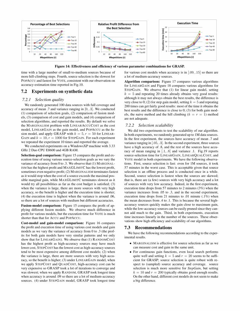
0
0.1
0.2
0.3
0.4
0.5
0.6
0.7
0.8
10 20 40 80 160 320
Pe
rce
nta
ge
#Repetitions (r)
Percentage of Best Selections
Top-5
Top-10
Top-20
Top-40
Top-80 0
0.05
0.1
0.15
0.2
10 20 40 80 160 320
Dif
fere
nce
#Repetitions (r)
Ralative Profit Difference from the Best Selection
Top-5
Top-10
Top-20
Top-40
Top-80 0
5
10
15
20
25
10 20 40 80 160 320
Exe
cuti
no
tim
e (
min
)
#Repetitions (r)
Execution Time
Top-5
Top-10
Top-20
Top-40
Top-80
Figure 14: Effectiveness and efficiency of various parameter combinations for GRASP.
time with a large number of small-to-medium sources because ofmore hill-climbing steps. Fourth, source selection is the slowest forPOPACCU and fastest for VOTE, consistent with our observation onaccuracy-estimation time reported in Fig.10.
7.2 Experiments on synthetic data
7.2.1 Selection qualityWe randomly generated 100 data sources with full coverage and
accuracy of mean .7 and variance ranging in [0, .3]. We conducted(1) comparison of selection goals, (2) comparison of fusion mod-els, (3) comparison of cost and gain models, and (4) comparison ofselection algorithms, and reported the results. By default we solvethe MARGINALISM problem with LINEARACCUCOST as the costmodel, LINEARGAIN as the gain model, and POPACCU as the fu-sion model, and apply GRASP with k = 5, r = 50 for LINEAR-GAIN and k = 10, r = 1000 for STEPGAIN. For each experimentwe repeated the experiment 10 times and reported the average.
We conducted experiments on a WindowsXP machine with 3.33GHz 2 Duo CPU E8600 and 4GB RAM.Selection-goal comparison: Figure 15 compares the profit and ex-ecution time of using various source-selection goals as we vary thevariance of accuracy from 0 to .3. We observe that (1) MARGINAL-ISM has the highest profit and MAXGLIMITC has the lowest profit,sometimes even negative profit; (2) MARGINALISM terminates fastestas it would stop when the cost of a source exceeds the maximal pos-sible marginal gain, while MAXGLIMITC terminates slowest as itwould try all possibilities as far as the cost budget is satisfied; (3)when the variance is large, there are more sources with very highaccuracy, so the benefit is higher and the execution time is shorter;(4) the execution time is highest when the variance is around .06,so there are a lot of sources with medium but different accuracies.Fusion-model comparison: Figure 15 compares the profit of ap-plying different fusion models. We observe much difference inprofit for various models, but the execution time for VOTE is muchshorter than that for ACCU and POPACCU.Cost-model and gain-model comparison: Figure 16 comparesthe profit and execution time of using various cost models and gainmodels as we vary the variance of accuracy from 0 to .3 (the prof-its for both gain models have very similar patterns and we onlyshow that for LINEARGAIN). We observe that (1) RANDOMCOSThas the highest profit as high-accuracy sources may have muchlower cost, STEPCOST has the lowest cost as high-accuracy sourcestend to be most expensive among different cost models; (2) whenthe variance is large, there are more sources with very high accu-racy, so the benefit is higher; (3) under LINEARGAIN model, whenwe apply STEPCOST and QUADCOST, high-accuracy cost can bevery expensive so GRASP took a lot of iterations to converge andwas slowest; when we apply RANDOM, GRASP took longest timewhen accuracy is around .09 so there are a lot of medium-accuracysources. (4) under STEPGAIN model, GRASP took longest time
for various cost models when accuracy is in [.09, .15] so there area lot of medium-accuracy sources.Algorithm comparison: Figure 17 compares various algorithmsfor LINEARGAIN and Figure 18 compares various algorithms forSTEPGAIN. We observe that (1) for linear gain model, settingk = 5 and repeating 20 times already obtains very good results:although it may not always obtain the best results, the difference isvery close to 0; (2) for step gain model, setting k = 5 and repeating200 times can get fairly good results: most of the time it obtains thebest results and the difference is close to 0; (3) for both gain mod-els, the naive method and the hill climbing (k = r = 1) methodare not adequate.
7.2.2 Selection scalabilityWe did two experiments to test the scalability of our algorithm.
In both experiments, we randomly generated up to 1M data sources.In the first experiment, the sources have accuracy of mean .7 andvariance ranging in [.05, .3]. In the second experiment, three sourceshave a high accuracy of .8, and the rest of the sources have accu-racy of mean ranging in [.1, .8] and variance .1. Fig.19 reportssource-selection time for LINEARGAIN, LINEARQUALCOST, andVOTE model in both experiments. We have the following observa-tions. First, source selection is fast: even for 1M sources, it took57 minutes in the worst case. This is acceptable given that sourceselection is an offline process and is conducted once in a while.Second, source selection is fastest when the sources are skewed;that is, there are (a few) sources with very high accuracy and a lotof sources with very low accuracy. Indeed, in the first experiment,execution time drops from 57 minutes to 2 minutes (3%) when thevariance increases from .05 to .3, and in the second experiment,execution time drops from 21 minutes to .01 minute (.1%) whenthe mean decreases from .4 to .1. This is because the several high-accuracy sources quickly makes the gain close to maximum gain,while the low-accuracy sources can be easily pruned since they can-not add much to the gain. Third, in both experiments, executiontime increases linearly in the number of the sources. These obser-vations show high efficiency and scalability of our algorithms.
7.3 RecommendationsWe have the following recommendations according to the exper-
imental results.
• MARGINALISM is effective for source selection as far as wecan measure cost and gain in the same unit.
• For continuous gain functions, even local search performsquite well and setting k = 5 and r = 20 seems to be suffi-cient for GRASP; source selection is quite robust with re-spect to (sampled) source accuracy and coverage. sourceselection is much more sensitive for StepGain, but settingk = 10 and r = 200 typically obtains good enough results.On the other hand, different cost models do not seem to makea big difference.
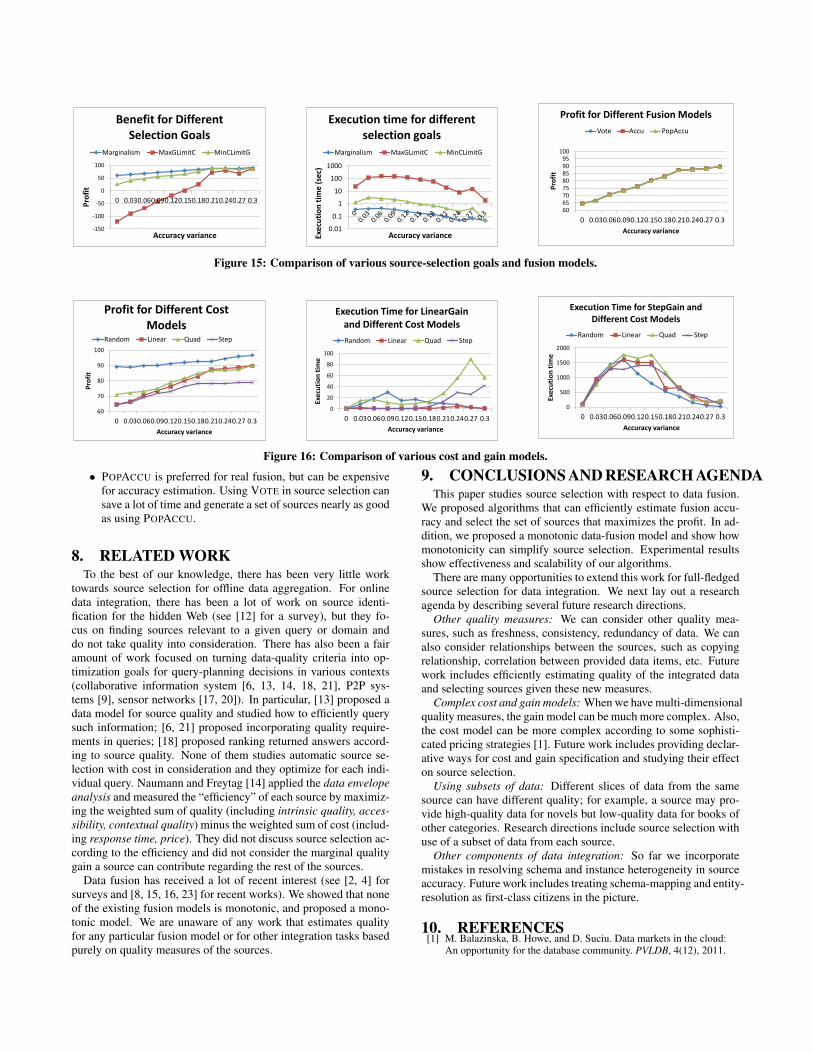
-150
-100
-50
0
50
100
0 0.03 0.06 0.09 0.12 0.15 0.18 0.21 0.24 0.27 0.3
Pro
fit
Accuracy variance
Benefit for Different Selection Goals
Marginalism MaxGLimitC MinCLimitG
0.01
0.1
1
10
100
1000
Exe
cuti
on
tim
e (
sec)
Accuracy variance
Execution time for different selection goals
Marginalism MaxGLimitC MinCLimitG
60 65 70 75 80 85 90 95
100
0 0.03 0.06 0.09 0.12 0.15 0.18 0.21 0.24 0.27 0.3
Pro
fit
Accuracy variance
Profit for Different Fusion Models
Vote Accu PopAccu
Figure 15: Comparison of various source-selection goals and fusion models.
60
70
80
90
100
0 0.03 0.06 0.09 0.12 0.15 0.18 0.21 0.24 0.27 0.3
Pro
fit
Accuracy variance
Profit for Different Cost Models
Random Linear Quad Step
0
20
40
60
80
100
0 0.03 0.06 0.09 0.12 0.15 0.18 0.21 0.24 0.27 0.3
Exe
cuti
on
tim
e
Accuracy variance
Execution Time for LinearGain and Different Cost Models
Random Linear Quad Step
0
500
1000
1500
2000
0 0.03 0.06 0.09 0.12 0.15 0.18 0.21 0.24 0.27 0.3
Exe
cuti
on
tim
e
Accuracy variance
Execution Time for StepGain and Different Cost Models
Random Linear Quad Step
Figure 16: Comparison of various cost and gain models.
• POPACCU is preferred for real fusion, but can be expensivefor accuracy estimation. Using VOTE in source selection cansave a lot of time and generate a set of sources nearly as goodas using POPACCU.
8. RELATED WORKTo the best of our knowledge, there has been very little work
towards source selection for offline data aggregation. For onlinedata integration, there has been a lot of work on source identi-fication for the hidden Web (see [12] for a survey), but they fo-cus on finding sources relevant to a given query or domain anddo not take quality into consideration. There has also been a fairamount of work focused on turning data-quality criteria into op-timization goals for query-planning decisions in various contexts(collaborative information system [6, 13, 14, 18, 21], P2P sys-tems [9], sensor networks [17, 20]). In particular, [13] proposed adata model for source quality and studied how to efficiently querysuch information; [6, 21] proposed incorporating quality require-ments in queries; [18] proposed ranking returned answers accord-ing to source quality. None of them studies automatic source se-lection with cost in consideration and they optimize for each indi-vidual query. Naumann and Freytag [14] applied the data envelopeanalysis and measured the “efficiency” of each source by maximiz-ing the weighted sum of quality (including intrinsic quality, acces-sibility, contextual quality) minus the weighted sum of cost (includ-ing response time, price). They did not discuss source selection ac-cording to the efficiency and did not consider the marginal qualitygain a source can contribute regarding the rest of the sources.
Data fusion has received a lot of recent interest (see [2, 4] forsurveys and [8, 15, 16, 23] for recent works). We showed that noneof the existing fusion models is monotonic, and proposed a mono-tonic model. We are unaware of any work that estimates qualityfor any particular fusion model or for other integration tasks basedpurely on quality measures of the sources.
9. CONCLUSIONS AND RESEARCH AGENDAThis paper studies source selection with respect to data fusion.
We proposed algorithms that can efficiently estimate fusion accu-racy and select the set of sources that maximizes the profit. In ad-dition, we proposed a monotonic data-fusion model and show howmonotonicity can simplify source selection. Experimental resultsshow effectiveness and scalability of our algorithms.
There are many opportunities to extend this work for full-fledgedsource selection for data integration. We next lay out a researchagenda by describing several future research directions.
Other quality measures: We can consider other quality mea-sures, such as freshness, consistency, redundancy of data. We canalso consider relationships between the sources, such as copyingrelationship, correlation between provided data items, etc. Futurework includes efficiently estimating quality of the integrated dataand selecting sources given these new measures.
Complex cost and gain models: When we have multi-dimensionalquality measures, the gain model can be much more complex. Also,the cost model can be more complex according to some sophisti-cated pricing strategies [1]. Future work includes providing declar-ative ways for cost and gain specification and studying their effecton source selection.
Using subsets of data: Different slices of data from the samesource can have different quality; for example, a source may pro-vide high-quality data for novels but low-quality data for books ofother categories. Research directions include source selection withuse of a subset of data from each source.
Other components of data integration: So far we incorporatemistakes in resolving schema and instance heterogeneity in sourceaccuracy. Future work includes treating schema-mapping and entity-resolution as first-class citizens in the picture.
10. REFERENCES[1] M. Balazinska, B. Howe, and D. Suciu. Data markets in the cloud:
An opportunity for the database community. PVLDB, 4(12), 2011.
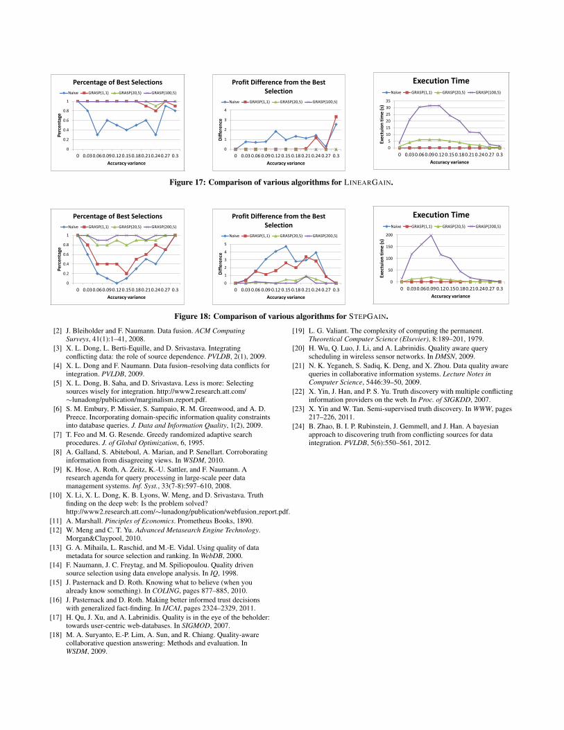
0
0.2
0.4
0.6
0.8
1
0 0.03 0.06 0.09 0.12 0.15 0.18 0.21 0.24 0.27 0.3
Pe
rce
nta
ge
Accuracy variance
Percentage of Best Selections
Naïve GRASP(1,1) GRASP(20,5) GRASP(100,5)
0
1
2
3
4
0 0.03 0.06 0.09 0.12 0.15 0.18 0.21 0.24 0.27 0.3
Dif
fere
nce
Accuracy variance
Profit Difference from the Best Selection
Naïve GRASP(1,1) GRASP(20,5) GRASP(100,5)
0
5
10
15
20
25
30
35
0 0.03 0.06 0.09 0.12 0.15 0.18 0.21 0.24 0.27 0.3
Exe
ctu
ion
tim
e (
s)
Accuracy variance
Execution Time Naïve GRASP(1,1) GRASP(20,5) GRASP(100,5)
Figure 17: Comparison of various algorithms for LINEARGAIN.
0
0.2
0.4
0.6
0.8
1
0 0.03 0.06 0.09 0.12 0.15 0.18 0.21 0.24 0.27 0.3
Pe
rce
nta
ge
Accuracy variance
Percentage of Best Selections
Naïve GRASP(1,1) GRASP(20,5) GRASP(200,5)
0
1
2
3
4
5
0 0.03 0.06 0.09 0.12 0.15 0.18 0.21 0.24 0.27 0.3
Dif
fere
nce
Accuracy variance
Profit Difference from the Best Selection
Naïve GRASP(1,1) GRASP(20,5) GRASP(200,5)
0
50
100
150
200
0 0.03 0.06 0.09 0.12 0.15 0.18 0.21 0.24 0.27 0.3
Exe
ctu
ion
tim
e (
s)
Accuracy variance
Execution Time Naïve GRASP(1,1) GRASP(20,5) GRASP(200,5)
Figure 18: Comparison of various algorithms for STEPGAIN.
[2] J. Bleiholder and F. Naumann. Data fusion. ACM ComputingSurveys, 41(1):1–41, 2008.
[3] X. L. Dong, L. Berti-Equille, and D. Srivastava. Integratingconflicting data: the role of source dependence. PVLDB, 2(1), 2009.
[4] X. L. Dong and F. Naumann. Data fusion–resolving data conflicts forintegration. PVLDB, 2009.
[5] X. L. Dong, B. Saha, and D. Srivastava. Less is more: Selectingsources wisely for integration. http://www2.research.att.com/∼lunadong/publication/marginalism report.pdf.
[6] S. M. Embury, P. Missier, S. Sampaio, R. M. Greenwood, and A. D.Preece. Incorporating domain-specific information quality constraintsinto database queries. J. Data and Information Quality, 1(2), 2009.
[7] T. Feo and M. G. Resende. Greedy randomized adaptive searchprocedures. J. of Global Optimization, 6, 1995.
[8] A. Galland, S. Abiteboul, A. Marian, and P. Senellart. Corroboratinginformation from disagreeing views. In WSDM, 2010.
[9] K. Hose, A. Roth, A. Zeitz, K.-U. Sattler, and F. Naumann. Aresearch agenda for query processing in large-scale peer datamanagement systems. Inf. Syst., 33(7-8):597–610, 2008.
[10] X. Li, X. L. Dong, K. B. Lyons, W. Meng, and D. Srivastava. Truthfinding on the deep web: Is the problem solved?http://www2.research.att.com/∼lunadong/publication/webfusion report.pdf.
[11] A. Marshall. Pinciples of Economics. Prometheus Books, 1890.[12] W. Meng and C. T. Yu. Advanced Metasearch Engine Technology.
Morgan&Claypool, 2010.[13] G. A. Mihaila, L. Raschid, and M.-E. Vidal. Using quality of data
metadata for source selection and ranking. In WebDB, 2000.[14] F. Naumann, J. C. Freytag, and M. Spiliopoulou. Quality driven
source selection using data envelope analysis. In IQ, 1998.[15] J. Pasternack and D. Roth. Knowing what to believe (when you
already know something). In COLING, pages 877–885, 2010.[16] J. Pasternack and D. Roth. Making better informed trust decisions
with generalized fact-finding. In IJCAI, pages 2324–2329, 2011.[17] H. Qu, J. Xu, and A. Labrinidis. Quality is in the eye of the beholder:
towards user-centric web-databases. In SIGMOD, 2007.[18] M. A. Suryanto, E.-P. Lim, A. Sun, and R. Chiang. Quality-aware
collaborative question answering: Methods and evaluation. InWSDM, 2009.
[19] L. G. Valiant. The complexity of computing the permanent.Theoretical Computer Science (Elsevier), 8:189–201, 1979.
[20] H. Wu, Q. Luo, J. Li, and A. Labrinidis. Quality aware queryscheduling in wireless sensor networks. In DMSN, 2009.
[21] N. K. Yeganeh, S. Sadiq, K. Deng, and X. Zhou. Data quality awarequeries in collaborative information systems. Lecture Notes inComputer Science, 5446:39–50, 2009.
[22] X. Yin, J. Han, and P. S. Yu. Truth discovery with multiple conflictinginformation providers on the web. In Proc. of SIGKDD, 2007.
[23] X. Yin and W. Tan. Semi-supervised truth discovery. In WWW, pages217–226, 2011.
[24] B. Zhao, B. I. P. Rubinstein, J. Gemmell, and J. Han. A bayesianapproach to discovering truth from conflicting sources for dataintegration. PVLDB, 5(6):550–561, 2012.
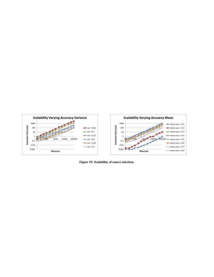
0.001
0.01
0.1
1
10
100
1000
100 1000 10000 100000 1000000
Exe
cuti
on
tim
e (s
ec)
#Sources
Scalability Varying Accuracy Variance
var = 0.05
var = 0.1
var = 0.15
var = 0.2
var = 0.25
var = 0.3 0.001
0.01
0.1
1
10
100
1000
100 1000 10000 100000 1000000
Exec
uti
on
tim
e (s
ec)
#Sources
Scalability Varying Accuarcy Mean
mean accu = 0.1
mean accu = 0.2
mean accu = 0.3
mean accu = 0.4
mean accu = 0.5
mean accu = 0.6
mean accu = 0.7
mean accu = 0.8
Figure 19: Scalability of source selection.