Lesson 13 - 1

Comparing Two Means

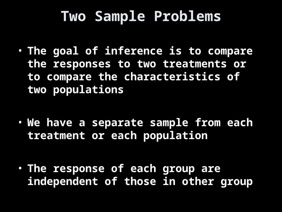
Two Sample Problems

• The goal of inference is to compare the responses to two treatments or to compare the characteristics of two populations

• We have a separate sample from each treatment or each population

• The response of each group are independent of those in other group

Conditions for Comparing 2 Means

• SRS– Two SRS’s from two distinct populations– Measure same variable from both populations

• Normality– Both populations are Normally distributed– In practice, (large sample sizes for CLT to apply)

similar shapes with no strong outliers

• Independence– Samples are independent of each other– Ni ≥ 10ni

2-Sample z Statistic

Facts about sampling distribution of x1 – x2

• Mean of x1 – x2 is 1 - 2 (since sample means are an unbiased estimator)

• Variance of the difference of x1 – x2 is

If the two population distributions are Normal, then so is the distribution of x1 – x2

σ1 σ2--- + ---n1 n2

² ²

2-Sample z Statistic

• Since we almost never know the population standard deviation (or for sure that the populations are normal), we very rarely use this in practice.

2-Sample t Statistic

Since we don’t know the standard deviations we use the t-distribution for our test statistic. But we have a problem with calculating the degrees of freedom! We have two options:•Let our calculator handle the complex calculations and tell us what the degrees of freedom are

•Use the smaller of n1 – 1 and n2 – 1 as a conservative estimate of the degrees of freedom

Classical and P-Value Approach – Two Means

Test Statistic:

tα-tα/2 tα/2-tα

Critical Region

P-Value is the area highlighted

|t0|-|t0|t0 t0

Reject null hypothesis, if

P-value < α

Left-Tailed Two-Tailed Right-Tailed

t0 < - tα

t0 < - tα/2

ort0 > tα/2

t0 > tα

Remember to add the areas in the two-tailed!

(x1 – x2) – (μ1 – μ2 ) t0 = ------------------------------- s1

2 s22

----- + ----- n1 n2

t-Test Statistic

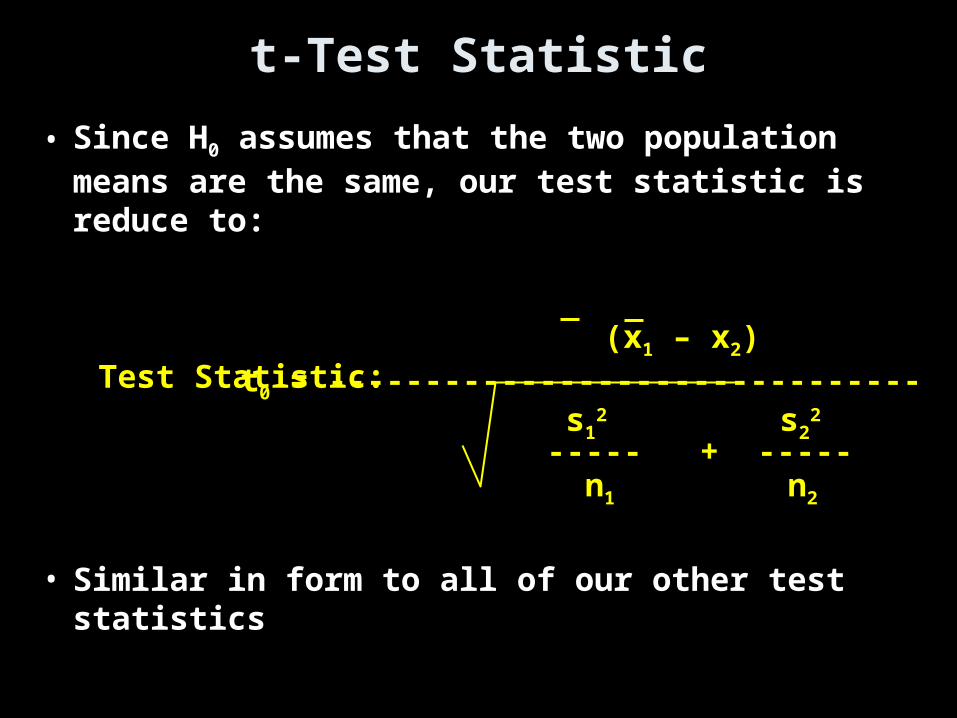
• Since H0 assumes that the two population means are the same, our test statistic is reduce to:

• Similar in form to all of our other test statistics

Test Statistic: (x1 – x2) t0 = ------------------------------- s1

2 s22

----- + ----- n1 n2

Confidence Intervals

Lower Bound:

Upper Bound:

tα/2 is determined using the smaller of n1 -1 or n2 -1 degrees of freedom

x1 and x2 are the means of the two samples

s1 and s2 are the standard deviations of the two samples

Note: The two populations need to be normally distributed or the sample sizes large

(x1 – x2) – tα/2 · s1

2 s22

----- + ----- n1 n2

(x1 – x2) + tα/2 · s1

2 s22

----- + ----- n1 n2

PE ± MOE

Two-sample, independent, T-Test on TI

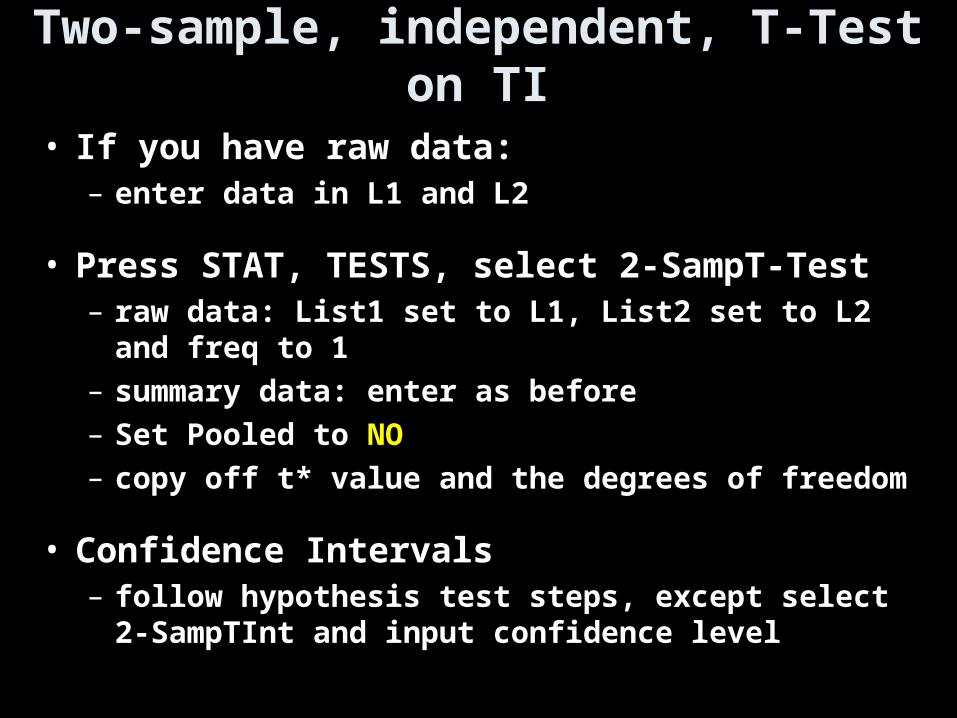
• If you have raw data:– enter data in L1 and L2

• Press STAT, TESTS, select 2-SampT-Test– raw data: List1 set to L1, List2 set to L2 and freq to

1– summary data: enter as before– Set Pooled to NO– copy off t* value and the degrees of freedom

• Confidence Intervals– follow hypothesis test steps, except select 2-

SampTInt and input confidence level

Inference Toolbox Review

• Step 1: Hypothesis– Identify population of interest and parameter

– State H0 and Ha

• Step 2: Conditions– Check appropriate conditions

• Step 3: Calculations– State test or test statistic– Use calculator to calculate test statistic and p-value

• Step 4: Interpretation– Interpret the p-value (fail-to-reject or reject)– Don’t forget 3 C’s: conclusion, connection and

context

Example 1Does increasing the amount of calcium in our diet reduce blood pressure? Subjects in the experiment were 21 healthy black men. A randomly chosen group of 10 received a calcium supplement for 12 weeks. The control group of 11 men received a placebo pill that looked identical. The response variable is the decrease in systolic (top #) blood pressure for a subject after 12 weeks, in millimeters of mercury. An increase appears as a negative response. Data summarized below

A)Calculate the summary statistics.

B)Test the claim

Subjects 1 2 3 4 5 6 7 8 9 10 11

Calcium 7 -4 18 17 -3 -5 1 10 11 -2 ----

Control -1 12 -1 -3 3 -5 5 2 -11 -1 -3

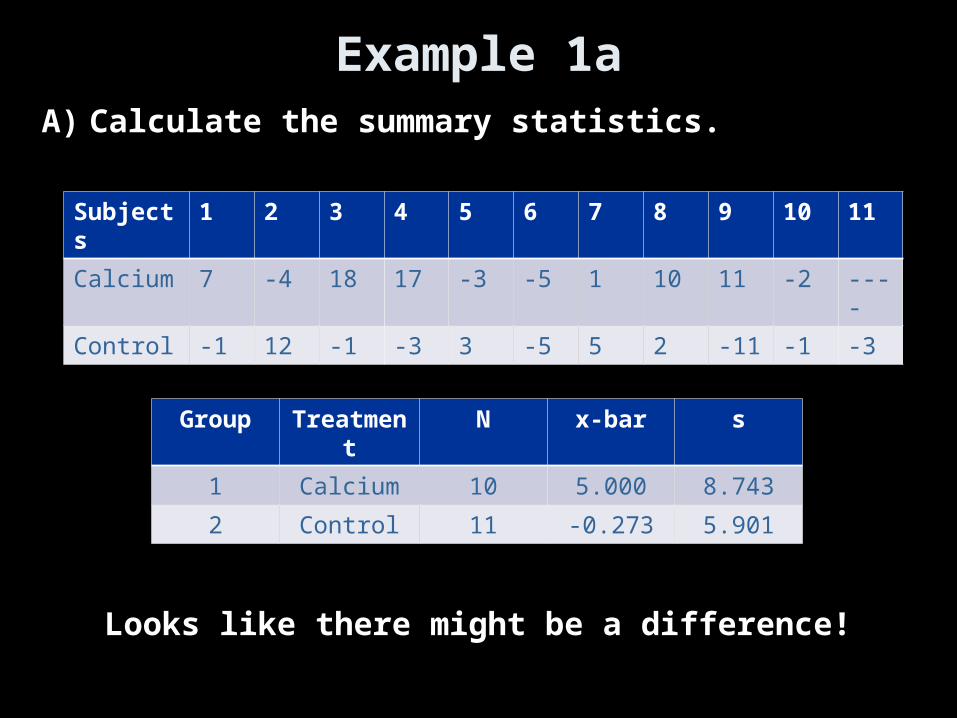
Example 1aA) Calculate the summary statistics.

Subjects 1 2 3 4 5 6 7 8 9 10 11

Calcium 7 -4 18 17 -3 -5 1 10 11 -2 ----

Control -1 12 -1 -3 3 -5 5 2 -11 -1 -3

Group Treatment N x-bar s

1 Calcium 10 5.000 8.743

2 Control 11 -0.273 5.901

Looks like there might be a difference!

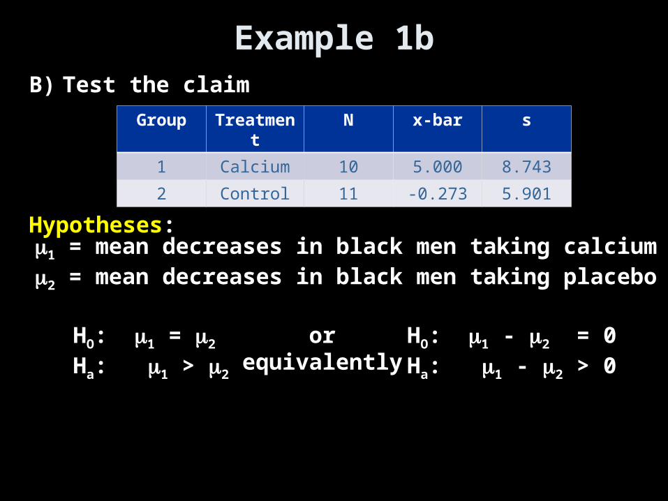
Example 1bB) Test the claim

Hypotheses:

Group Treatment N x-bar s

1 Calcium 10 5.000 8.743

2 Control 11 -0.273 5.901

HO: 1 = 2

Ha: 1 > 2

1 = mean decreases in black men taking calcium2 = mean decreases in black men taking placebo

HO: 1 - 2 = 0Ha: 1 - 2 > 0

orequivalently

Example 1b contConditions:

SRS

Normality

Independence

The 21 subjects were not a random selection from all healthy black men. Hard to generalize to that population any findings. Random assignment of subjects to treatments should ensure differences due to treatments only.

Sample size too small for CLT to apply; Plots Ok.

Because of the randomization, the groups can be treated as two independent samples

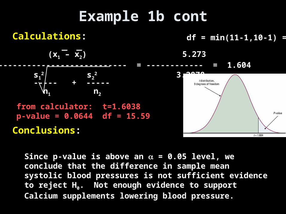
Example 1b contCalculations:

Conclusions:

(x1 – x2) 5.273t0 = ------------------------------- = ------------ = 1.604 s1

2 s22 3.2878

----- + ----- n1 n2

df = min(11-1,10-1) = 9

from calculator: t=1.6038 p-value = 0.0644 df = 15.59

Since p-value is above an = 0.05 level, we conclude that the difference in sample mean systolic blood pressures is not sufficient evidence to reject H0. Not enough evidence to support Calcium supplements lowering blood pressure.

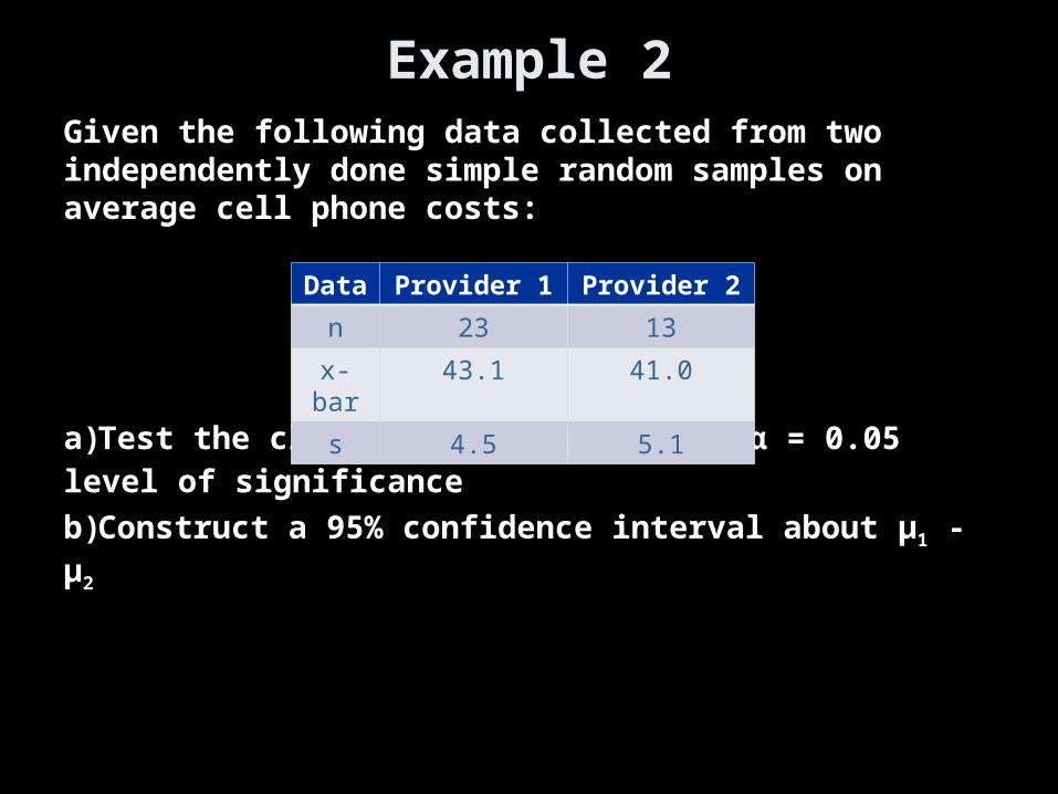
Example 2Given the following data collected from two independently done simple random samples on average cell phone costs:

a)Test the claim that μ1 > μ2 at the α = 0.05 level of significance

b)Construct a 95% confidence interval about μ1 - μ2

Data Provider 1 Provider 2

n 23 13

x-bar 43.1 41.0

s 4.5 5.1

Example 2a Cont• Parameters

• HypothesisH0: H1:

• Requirements:SRS:

Normality:

Independence:

μ1 > μ2 (Provider 1 costs more than Provider 2)

μ1 = μ2 (No difference in average costs)

ui is average cell phone cost for provider i

Stated in the problem

Have to assume to work the problem. Sample size to small for CLT to apply

Stated in the problem

Example 2a Cont

• Calculation:

Critical Value:

• Conclusion:

tc(13-1,0.05) = 1.782, α = 0.05

Since the p-value > (or that tc > t0), we would not have evidence to reject H0. The cell phone providers average costs seem to be the same.

= 1.237, p-value = 0.1144 x1 – x2 - 0t0 = ------------------------ (s²1/n1) + (s²2/n2)

Example 2b

• Confidence Interval: PE ± MOE

[ -1.5986, 5.7986] by hand

(x1 – x2) ± tα/2 · s1

2 s22

----- + ----- n1 n2

tc(13-1,0.025) = 2.179

2.1 ± 2.179 (20.25/23) + (26.01/13)

2.1 ± 2.179 (1.6974) = 2.1 ± 3.6986

[ -1.4166, 5.6156] by calculator

It uses a different way to calculate the degrees of freedom (as shown on pg 792)

DF - Welch and Satterthwaite Apx

• Using this approximation results in narrower confidence intervals and smaller p-values than the conservative approach mentioned before

Pooling Standard Deviations??

• DON’T

• Pooling assumes that the standard deviations of the two populations are equal – very hard to justify this

• This could be tested using the F-statistic (a non robust procedure beyond AP Stats)

• Beware: formula on AP Stat equation set under Descriptive Statistics

Summary and Homework

• Summary– Two sets of data are independent when observations

in one have no affect on observations in the other– Differences of the two means usually use a Student’s

t-test of mean differences– The overall process, other than the formula for the

standard error, are the general hypothesis test and confidence intervals process

• Homework– 13.1, 7, 8, 13, 17