Embed Size (px)
Citation preview

1
Lessons From Capital Market History:Return & Risk
Chapter 10
2
Topics• Calculate 1 Period Returns• Five Important Types of Financial Investments– Risk-Free Investment
• What We Can Learn From Capital Market History– Using Past To Predict Future– Average Returns: There Is Reward For Bearing Risk– Variability In Returns: The Greater The Potential Reward,
The Greater The Risk• Risk & Return• Arithmetic V Geometric Mean• Markets Are Only Efficient In The Long Run

3
1 Year Percent Return
t
ttt
t
tt
t
t
P
PPD
CGYDY
P
PPCGY
P
DDY
11
1
1
Return %
Return %
Dividend Yield
Capital Gains Yield
4
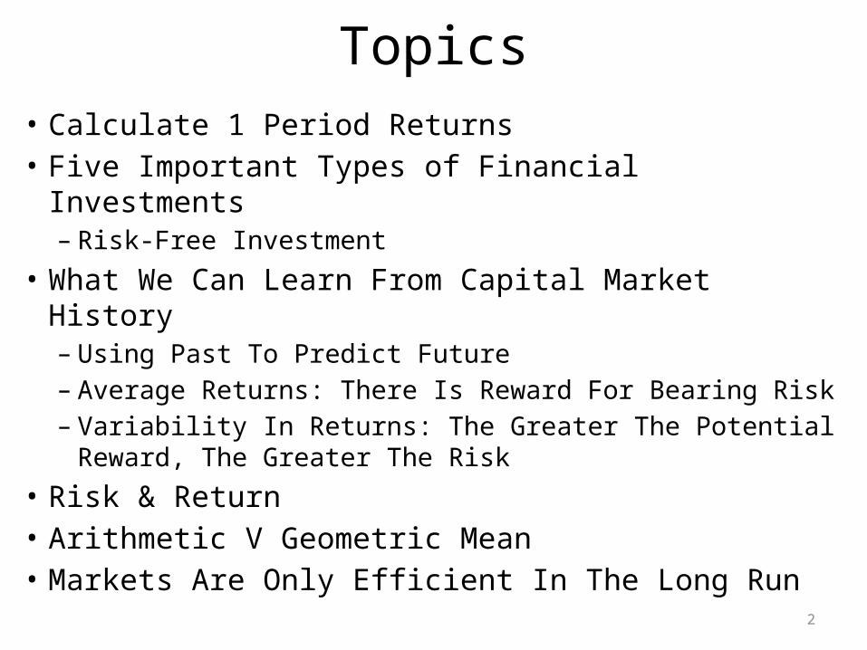
Period Returns = Holding Returns = 1 Year ReturnsReturns On Investment For 1 Year (Holding
Period Return)(Regardless of whether you sell the stock or
not)Stock Price Time 0 = (Beg) = Pt $25.00Stock Price Time 1 = (End) = Pt+1 $19.50Dividend Paid at Time 1 = Dt+1 $2.00Capital Gain = Pt+1 - Pt -$5.50Dollar Returns = Dividend Paid + Capital Gain -$3.50% Return = (Dollar Return)/(End Stock Price) -14.00%Dividend Yield = Dt+1/Pt 8.00%Capital Gain Yield = Pt+1/Pt - 1 -22.00%% Return = Dividend Yield + Capital Gain Yield -14.00%% Return + 1 = (Dt+1 + Pt+1)/Pt 86.00%
Returns On Investment For 1 Year (Holding Period Return)
(Regardless of whether you sell the stock or not)
Stock Price Time 0 = (Beg) = Pt $25.00Stock Price Time 1 = (End) = Pt+1 $26.00Dividend Paid at Time 1 = Dt+1 $2.00Capital Gain = Pt+1 - Pt $1.00Dollar Returns = Dividend Paid + Capital Gain $3.00% Return = (Dollar Return)/(End Stock Price) 12.00%Dividend Yield = Dt+1/Pt 8.00%Capital Gain Yield = Pt+1/Pt - 1 4.00%% Return = Dividend Yield + Capital Gain Yield 12.00%% Return + 1 = (Dt+1 + Pt+1)/Pt 112.00%

5
Five Important Types of Financial Investments• Roger Ibbotson & Rex Sinquefield did famous study that looked
at the nominal-pretax-returns for five important types of financial investments in US markets during the period 1926 - 2008:1. Large Company Stocks Portfolio based on S & P 500 Index (in terms of
MV of outstanding stock)2. Small Company Stocks Portfolio based on smallest 20% of companies
listed on NYSE (in terms of MV of outstanding stock)3. Long-term High Quality Corporate Bonds Portfolio (20 Years to
Maturity)4. Long-term US Government Bonds Portfolio (20 Years to maturity)5. US Treasury Bills (T-bills) with one-month maturity
• Virtually free of any default risk because government can raise taxes to pay bills, especially since the time frame is one monrth.
• T-bill return is considered the “risk-free return”
6
US Capital Market History• Looking at the past can perhaps provide some
insight into the future.• Using the past to predict the future can be
dangerous if the past isn’t representative of what the future will bring.– 2000 to 2007 people around the world looked at
past house prices to predict future house prices.– 1995 to 2000 people looked at past prices for
internet stocks prices to help predict future prices.

7
U.S. Financial Markets
The Historical Record: 1925-
2008

8
Year-to-Year Total Returns
Large-Company Stock Returns
9
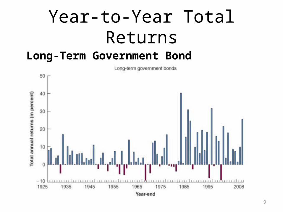
Year-to-Year Total Returns
Long-Term Government Bond Returns
10
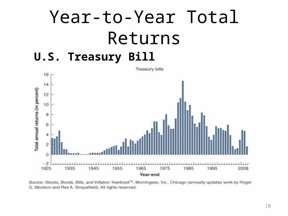
Year-to-Year Total Returns
U.S. Treasury Bill Returns

11
Year To Year Returns (Hand typed from tables in textbook)
YearLarge Company Stocks
Down Large Company Stocks
Long Term Government Bonds
Down Long Term Government Bonds US Treasury Bills
Consumer Price Index
1926 11.14% 7.90% 3.30% -1.12%1927 37.13% 10.36% 3.15% -2.26%1928 43.31% -1.37% -1.37% 4.05% -1.16%1929 -8.91% -8.91% 5.23% 4.47% 0.58%1930 -25.26% -25.26% 5.80% 2.27% -6.40%1931 -43.86% -43.86% -8.04% -8.04% 1.15% -9.32%1932 -8.85% -8.85% 14.11% 0.88% -10.27%1933 52.88% 31.00% 0.52% 0.76%1934 -2.34% -2.34% 12.98% 0.27% 1.52%1935 47.22% 5.88% 0.17% 2.99%1936 32.80% 8.22% 0.17% 1.45%1937 -35.26% -35.26% -0.13% -0.13% 0.27% 2.86%1938 33.20% 6.26% 0.06% -2.78%1939 -0.91% -0.91% 5.71% 0.04% 0.00%1940 -10.08% -10.08% 10.34% 0.04% 0.71%1941 -11.77% -11.77% -8.66% -8.66% 0.14% 9.93%1942 21.07% 2.67% 0.34% 9.03%1943 25.76% 2.50% 0.38% 2.96%1944 19.69% 2.88% 0.38% 2.30%1945 36.46% 5.17% 0.38% 2.25%1946 -8.18% -8.18% 4.07% 0.38% 18.13%1947 5.24% -1.15% -1.15% 0.62% 8.84%1948 5.10% 2.10% 1.06% 2.99%1949 18.06% 7.02% 1.12% -2.07%1950 30.58% -1.44% -1.44% 1.22% 5.93%1951 24.55% -3.53% -3.53% 1.56% 6.00%1952 18.50% 1.82% 1.75% 0.75%1953 -1.10% -1.10% -0.88% -0.88% 1.87% 0.75%1954 52.40% 7.89% 93.00% -0.74%1955 31.43% -1.03% -1.03% 1.80% 0.37%

12
Year To Year Returns (Hand typed from tables in textbook)
YearLarge Company Stocks
Down Large Company Stocks
Long Term Government Bonds
Down Long Term Government Bonds US Treasury Bills
Consumer Price Index
1956 6.63% -3.14% -3.14% 2.66% 2.99%1957 -10.85% -10.85% 5.25% 3.28% 2.90%1958 43.34% -6.70% -6.70% 1.71% 1.76%1959 11.90% -1.35% -1.35% 3.48% 1.73%1960 48.00% 7.74% 2.81% 1.36%1961 26.81% 3.02% 2.40% 0.67%1962 -8.78% -8.78% 4.63% 2.82% 1.33%1963 22.69% 1.37% 3.23% 1.64%1964 16.36% 4.43% 3.62% 0.97%1965 12.36% 1.40% 4.06% 1.92%1966 -10.10% -10.10% -1.61% -1.61% 4.94% 3.46%1967 23.94% -6.38% -6.38% 4.39% 3.04%1968 11.00% 5.33% 5.49% 4.72%1969 -8.47% -8.47% -7.45% -7.45% 6.90% 6.20%1970 3.94% 12.24% 6.50% 5.57%1971 14.30% 12.67% 4.36% 3.27%1972 18.99% 9.15% 4.23% 3.41%1973 -14.69% -14.69% -12.66% -12.66% 7.29% 8.71%1974 -26.47% -26.47% -3.28% -3.28% 7.99% 12.34%1975 37.23% 4.67% 5.87% 6.94%1976 23.93% 18.34% 5.07% 4.86%1977 -7.16% -7.16% 2.31% 5.45% 6.70%1978 6.57% -2.07% -2.07% 7.64% 9.02%1979 18.61% -2.76% -2.76% 10.56% 13.29%1980 32.50% -5.91% -5.91% 12.10% 12.52%1981 -4.92% -4.92% -0.16% -0.16% 14.60% 8.92%1982 21.55% 49.99% 10.94% 3.83%1983 22.56% -2.11% -2.11% 8.99% 3.79%1984 6.27% 16.53% 9.90% 3.95%1985 31.73% 39.03% 7.71% 3.80%

13
Year To Year Returns (Hand typed from tables in textbook)
YearLarge Company Stocks
Down Large Company Stocks
Long Term Government Bonds
Down Long Term Government Bonds US Treasury Bills
Consumer Price Index
1986 18.67% 32.51% 6.09% 1.10%1987 5.25% -8.09% -8.09% 5.88% 4.43%1988 16.61% 8.71% 6.94% 4.42%1989 31.69% 22.15% 8.44% 4.65%1990 -3.10% -3.10% 5.44% 7.69% 6.11%1991 30.46% 20.04% 5.43% 3.06%1992 7.62% 8.09% 3.48% 2.90%1993 10.08% 22.32% 3.03% 2.75%1994 1.32% -11.46% -11.46% 4.39% 2.67%1995 37.58% 37.28% 5.61% 2.54%1996 22.96% -2.59% -2.59% 5.14% 3.32%1997 33.36% 17.70% 5.19% 1.70%1998 28.58% 19.22% 4.86% 1.61%1999 21.04% -12.76% -12.76% 4.80% 2.68%2000 -9.10% -9.10% 22.16% 5.98% 3.39%2001 -11.89% -11.89% 5.30% 3.33% 1.55%2002 -22.10% -22.10% 14.08% 1.61% 2.38%2003 28.68% 1.62% 1.03% 1.88%2004 10.88% 10.34% 1.43% 3.26%2005 4.91% 10.35% 3.30% 3.42%2006 15.79% 28.00% 4.97% 2.54%2007 5.49% 10.85% 4.52% 4.08%2008 -37.00% -37.00% 39.46% 1.24% 0.09%

14
Arithmetic Mean = “Average”
• Arithmetic Mean =• Mean =• “Average” (everyday language) =• “Typical Value” =• One Value that Can Represent All The Values =
• (Add Then All Up)/Count

15
Historical Average Returns
• Historical Averages For Asset Classes = Arithmetic Mean of Asset Class = (Add then all up)/Count
• Reward For Risk = Risk Premium = Historical Arithmetic Mean of Asset Class – Historical Arithmetic Mean of T-Bill

16
Historical Averages, Reward For Risk, Real Rate
InvestmentHistorical Average Return = RH
RH - Rf = Reward For Risk
RH - I = Real Historical Rate
Large Stocks 11.70% 7.90% 8.60%Small Stocks 16.40% 12.60% 13.30%Long-term Corporate Bonds 6.20% 2.40% 3.10%Long-term Government Bonds 6.10% 2.30% 3.00%U.S. Treasury Bills = Rf 3.80% 0.00% 0.70%Inflation = I 3.10% 0.00%
• What We Can Learn From Capital Market History– Lesson 1: There Is Reward For Bearing Risk
•But why do some investments get more reward?– The answer lies in “variability of returns”

17
Variability In Returns = Volatility In Returns = Risk
• Variability seen with Line & Column Chart• Variability seen with X-Y scatter chart• Variability seen with Frequency Distribution• Risk Measured by calculating Standard
Deviation

18
U.S. Financial Markets
The Historical Record: 1925-
2008

19
Year-to-Year Total Returns
Large-Company Stock Returns

20
Year-to-Year Total Returns
Long-Term Government Bond Returns

21
Year-to-Year Total Returns
U.S. Treasury Bill Returns

22
Variability seen with X-Y scatter chart
Which set of data is more spread out?Which mean represents its data points more fairly?If the data points are all clustered around the mean, then there is less variability, less risk that your return will be different than the mean.

23
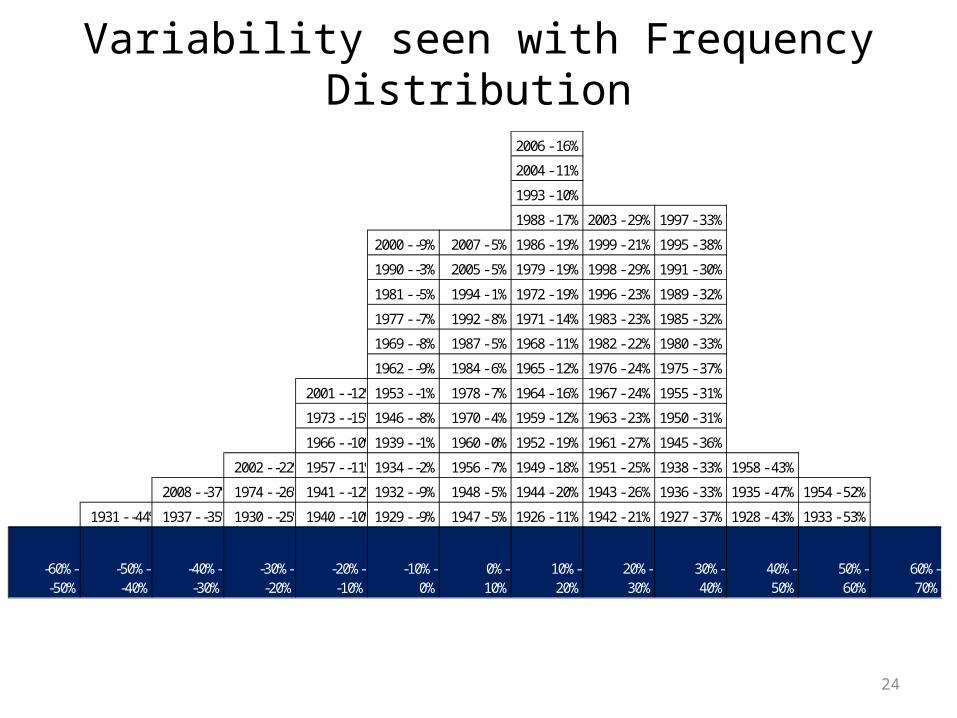
Variability seen with Frequency Distribution
24
Variability seen with Frequency Distribution
-60%--50%
-50%--40%
1931 - -44%
-40%--30%
1937 - -35%
2008 - -37%
-30%--20%
1930 - -25%
1974 - -26%
2002 - -22%
-20%--10%
1940 - -10%
1941 - -12%
1957 - -11%
1966 - -10%
1973 - -15%
2001 - -12%
-10%-0%
1929 - -9%
1932 - -9%
1934 - -2%
1939 - -1%
1946 - -8%
1953 - -1%
1962 - -9%
1969 - -8%
1977 - -7%
1981 - -5%
1990 - -3%
2000 - -9%
0%-10%
1947 - 5%
1948 - 5%
1956 - 7%
1960 - 0%
1970 - 4%
1978 - 7%
1984 - 6%
1987 - 5%
1992 - 8%
1994 - 1%
2005 - 5%
2007 - 5%
10%-20%
1926 - 11%
1944 - 20%
1949 - 18%
1952 - 19%
1959 - 12%
1964 - 16%
1965 - 12%
1968 - 11%
1971 - 14%
1972 - 19%
1979 - 19%
1986 - 19%
1988 - 17%
1993 - 10%
2004 - 11%
2006 - 16%
20%-30%
1942 - 21%
1943 - 26%
1951 - 25%
1961 - 27%
1963 - 23%
1967 - 24%
1976 - 24%
1982 - 22%
1983 - 23%
1996 - 23%
1998 - 29%
1999 - 21%
2003 - 29%
30%-40%
1927 - 37%
1936 - 33%
1938 - 33%
1945 - 36%
1950 - 31%
1955 - 31%
1975 - 37%
1980 - 33%
1985 - 32%
1989 - 32%
1991 - 30%
1995 - 38%
1997 - 33%
40%-50%
1928 - 43%
1935 - 47%
1958 - 43%
50%-60%
1933 - 53%
1954 - 52%
60%-70%

25
Which Stock Would You Prefer?Each Has a Mean Return Of 4.1%
Why?
Count 15Mean 4.1%Year Stock Return Deviation = R = Mean
1995 2.0% -2.1%1996 4.0% -0.1%1997 3.5% -0.6%1998 5.5% 1.4%1999 4.0% -0.1%2000 4.2% 0.1%2001 4.3% 0.2%2002 4.7% 0.6%2003 5.0% 0.9%2004 5.1% 1.0%2005 3.0% -1.1%2006 2.9% -1.2%2007 4.6% 0.5%2008 4.9% 0.8%2009 4.1% 0.0%
Total 0
Count 15Mean 4.1%Year Stock Return Deviation = R = Mean
1995 5.0% 0.9%1996 10.0% 5.9%1997 12.0% 7.9%1998 17.0% 12.9%1999 19.0% 14.9%2000 1.0% -3.1%2001 -15.0% -19.1%2002 -3.0% -7.1%2003 3.0% -1.1%2004 5.5% 1.4%2005 10.0% 5.9%2006 6.5% 2.4%2007 -2.0% -6.1%2008 -22.0% -26.1%2009 15.0% 10.9%
Total 0

26
Which Stock Would You Prefer?Each Has a Mean Return Of 4.1%
Why?

27
But Now We Need A Number To Measure The
Volatility of Returns

28
Variability Measured By Calculating Standard Deviation
• Risk is measured by the dispersion, spread, or volatility of returns.
• Standard Deviation will be calculated number that measures variability, or volatility, or dispersion, or simply RISK

29
How Far Does Each Actual Return Deviate From The Mean In A Typical Year?
• Deviation tells you how far each return is from the mean
• Deviation = Return – Mean• If we average these deviations, it will
give us an indication of the volatility of the stock.
• Sum of Deviations = 0• This means we can’t calculate the
mean in the normal way.
Mean 4.1%
Year Stock Return Deviation1995 5.0% 0.9%1996 10.0% 5.9%1997 12.0% 7.9%1998 17.0% 12.9%1999 19.0% 14.9%2000 1.0% -3.1%2001 -15.0% -19.1%2002 -3.0% -7.1%2003 3.0% -1.1%2004 5.5% 1.4%2005 10.0% 5.9%2006 6.5% 2.4%2007 -2.0% -6.1%2008 -22.0% -26.1%2009 15.0% 10.9%
Total 0

30
Standard Deviation Is A Numerical Measure Of Volatility Or “Risk” Of Stock

31
Standard Deviation Is A Numerical Measure Of Volatility Or “Risk” Of Stock

32
What We Can Learn From Capital Market HistoryLesson 2: The Greater The Potential Reward, The Greater The Risk

33
Standard Normal CurveDo Our Historical Distributions Look Bell Shaped?

34
Risk And The Standard Normal CurveOnly Past Distributions That Fit The “Normal” Curve Can Use The
Standard Normal Curve
• Normal distribution: – A symmetric frequency distribution – The “bell-shaped curve”– Completely described by the mean and variance
• Example: Mean = 11.7%, Standard Deviation = 20.6%, the 68% of the values should lie between 11.7%-20.6% and 11.7% + 20.6% or -8.9% and 32.3%.

35
If Assume Bell Shaped
If bell shaped Distributions68% chance that in any given year
the returns will lie between:
InvestmentHistorical Average Return = RH
Stabndard Devaition (risk) Lower Upper
Large Stocks 11.70% 20.60% -8.90% 32.30%Small Stocks 16.40% 33.00% -16.60% 49.40%Long-term Corporate Bonds 6.20% 8.40% -2.20% 14.60%Long-term Government Bonds 6.10% 9.40% -3.30% 15.50%U.S. Treasury Bills = Rf 3.80% 3.10% 0.70% 6.90%Inflation = I 3.10% 4.20% -1.10% 7.30%
10-36
Risk–Return Tradeoff(Conclusion To Chapter 10)
• Two key lessons from capital market history: – There is a reward for bearing risk– The greater the potential reward, the
greater the risk
37
Capital Market History
• Average Returns: There Is Reward For Bearing Risk
• Variability In Returns: The Greater The Potential Reward, The Greater The Risk
38
Mean Return & Standard Deviation
• For Historical Returns we use Mean & Standard Deviation
• For Projected Future Returns we use “Expected Returns” based probability theory to calculate returns and risk (standard deviation). Chapter 11

10-39
Arithmetic vs. Geometric Mean• Arithmetic average: – Return earned in an average period over multiple periods– Answers the question: “What was your return in an
average year over a particular period?”• Geometric average: – Average compound return per period over multiple
periods– Answers the question: “What was your average compound
return per year over a particular period?”
• Geometric average < arithmetic average unless all the returns are equal
10-40
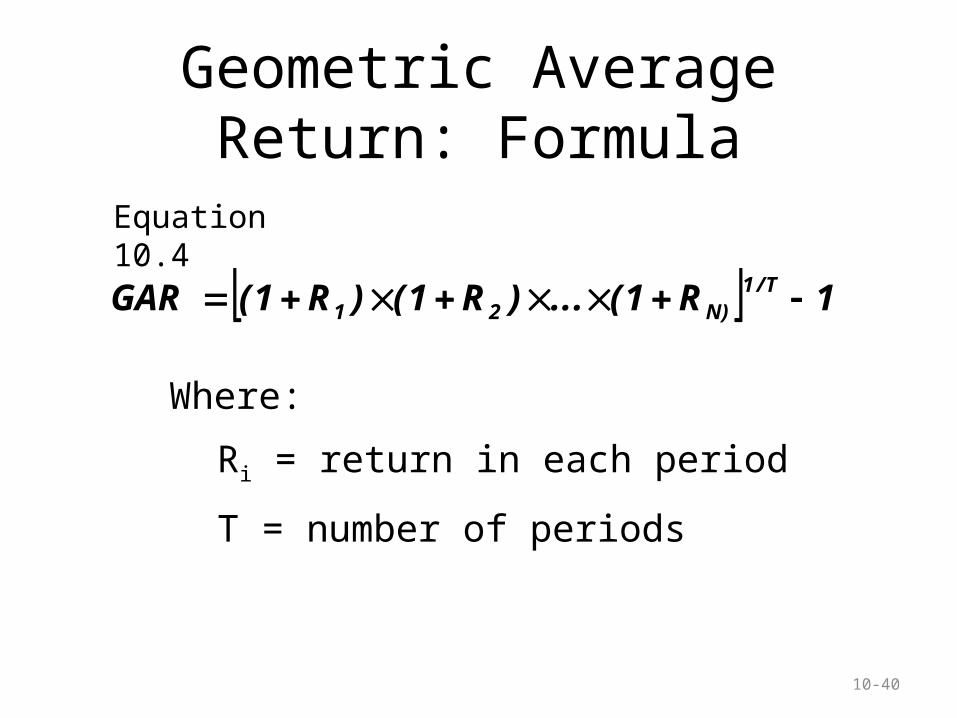
Geometric Average Return: Formula
1R1(...)R1()R1(GAR /T1N)21
Where:
Ri = return in each period
T = number of periods
Equation 10.4

10-41
Arithmetic vs. Geometric MeanWhich is better?
• The arithmetic average is overly optimistic for long horizons
• The geometric average is overly pessimistic for short horizons
• Depends on the planning period under consideration• 15 – 20 years or less: use arithmetic• 20 – 40 years or so: split the difference between them• 40 + years: use the geometric

42
Efficient Markets Hypothesis• Efficient Markets = new information is assimilated quickly &
correctly into financial asset prices. The correctly priced assets help to efficiently allocate resources in the capitalist system.
• Financial Markets are efficient in that when new information becomes available, people buying and selling stocks and bonds try to incorporate new information into their estimates of the security.– Competition between investors means that people study companies
very closely, trying to find the mispriced stock. When everyone is doing this, prices tend to be not mispriced.
– EMH implies that all investments are NPV = 0. This is because if prices are not too high or low:• NPV (investors estimate) – MV (Price in market) = 0

43
Efficient Markets Hypothesis
• Strong Efficient– All public and private info is reflected in security price.
• Semistrong Efficient• All public info is reflected in security price.• If true, financial statement analysis or studying current
mortgage rate defaults is futile.– People study info like this all the time.
– Weak Form Efficient• Past Security Price info is reflected in security price.
– If true, searching for patterns in historical prices is futile.– People do this all the time “Technical Analysis”.

44
Efficient Markets Theory As Currently Stated Is False
• Herd mentality or “animal spirits” tend to make people follow certain trends in the market even when the trend is unreasonable (1990 Internet Stocks, 2000 Housing Prices). Fisher, Keynes and Minsky all wrote extensively about such behavior.
• Often times Financial Market Bubbles are fueled by firms and individuals borrowing money to buy up assets, the increased demand for assets increases the price of the assets, the increased value of the assets allows people to borrow more because they have more collateral. In essence, “easy credit” can contribute to assets price increases that do not reflect the underlying fundamentals of the asset.– Examples: Depression and the 2007-2010 Housing Crisis.– 2007-2010 Housing Crisis: housing prices where well above the present
value of future rent cash flows.

45
Efficient Markets Theory As Currently Stated Is False
• The idea that markets always price financial assets correctly has been proven false a number of times in history.– Example: Public information about default rates on houses was
available in the years 2005 - 2007, and yet prices on mortgage back securities did not adjust downward until late 2007. As a result of the overpriced financial assets, people continued to take out loans and buy houses. This is an example of how resources are inefficiently allocated when prices are not correct based on inefficient markets. The result: many people got seriously hurt when the prices finally did adjust (late).
– AOL was priced high at the height of the Internet Bubble in the late 1990s.
– If markets are efficient, how come AOL stock was valued so high for so long? How come mortgage backed securities with loans from 2004 – 2007 had a price at all?

46
Efficient Markets Are Only Efficient In The Long Run
• In the long run, markets tend to be efficient (eventually, internet stocks and mortgage back securities did fall).