Embed Size (px)
Citation preview

U.S. ENVIRONMENTAL PROTECTION AGENCY (EPA) & MAJOR PARTNERS’
LESSONS LEARNED FROM IMPLEMENTING EPA’S PORTION OF THE
AMERICAN RECOVERY AND REINVESTMENT ACT:
FACTORS AFFECTING IMPLEMENTATION AND PROGRAM SUCCESS
ECONOMIC IMPACTS OF LEVERAGED PROJECTS ON LOCALITIES
SEPTEMBER 2013
EPA-100-K-13-010
PREPARED FOR
U.S. ENVIRONMENTAL PROTECTION AGENCY
OFFICE OF THE CHIEF FINANCIAL OFFICER
WASHINGTON, DC


ACKNOWLEDGEMENTS
This study could not have been possible without the help and cooperation of the many U.S. Environmental Protection Agency (EPA) employees at Headquarters and Regional offices who agreed to be interviewed, state staff and funding recipients who participated in lively focus group sessions, and the many other EPA and state staff who graciously provided answers to follow-up questions after the interviews and focus groups were completed. The Science Applications International Corporation (SAIC) Team appreciates the time given to share experiences beyond all the other audits and questions. The recollections of those ‘working in the trenches’ during the intense period of American Recovery and Reinvestment Act (ARRA) implementation were invaluable in this study.
September 2013 i

This page intentionally blank.
September 2013 ii

TABLE OF CONTENTS
EXECUTIVE SUMMARY ................................................................................................................ 1
PURPOSE ................................................................................................................................... 1 METHODOLOGY........................................................................................................................... 1 FINDINGS ................................................................................................................................... 2
SECTION 1. INTRODUCTION .................................................................................................. 3
1.1 BACKGROUND AND OBJECTIVES OF THIS STUDY ........................................................................ 3 1.2 STUDY QUESTIONS ............................................................................................................. 4
SECTION 2. METHODOLOGY AND DATA SOURCES ................................................................ 7
2.1 STUDY DESIGN .................................................................................................................. 7 2.2 CASE STUDY SELECTION ...................................................................................................... 8 2.3 CASE STUDY DATA COLLECTION .......................................................................................... 10 2.4 QUALITATIVE ANALYSIS – ENVIRONMENTAL AND HEALTH RISK REDUCTION BENEFITS ..................... 11 2.5 QUANTITATIVE ANALYSIS – REGIONAL ECONOMIC IMPACT MODELING ........................................ 12 2.6 STUDY LIMITATIONS ......................................................................................................... 13
SECTION 3. FINDINGS.......................................................................................................... 15
3.1 RESULTS OF QUALITATIVE ECONOMIC AND ENVIRONMENTAL IMPACT REVIEW .............................. 16 3.2 RESULTS OF QUANTITATIVE REGIONAL ECONOMIC IMPACT MODELING ....................................... 18
3.2.1 Variations in Local Expenditures ........................................................................... 19 3.2.2 Variations in RIMS II Modeling Results .................................................................. 21 3.2.3 Variations in Funding Leverage ............................................................................. 27
REFERENCES ............................................................................................................................. 29
September 2013 iii

TABLES
TABLE 1. STUDY QUESTIONS AND CORRESPONDING RESEARCH QUESTIONS.................................................. 5 TABLE 2. CHARACTERISTICS USED TO CATEGORIZE ARRA PROJECTS FOR CASE STUDY SELECTION ..................... 9 TABLE 3. CASE STUDY PROJECT LOCATION AND DESCRIPTION.................................................................... 9 TABLE 4. CASE STUDY PROJECTS BY PROGRAM AND SELECTION CATEGORY ................................................ 10 TABLE 5. DATA REQUIREMENTS AND SOURCES .................................................................................... 11 TABLE 6. EXAMPLE OF MULTIPLIER ANALYSIS INPUTS AND OUTPUTS (SANTA CRUZ COUNTY) ........................ 13 TABLE 7. STUDY QUESTIONS WITH BIG PICTURE FINDINGS ..................................................................... 15 TABLE 8. MEDIUM- AND LONG-TERM BENEFITS OF PROJECT .................................................................. 17 TABLE 9. CASE STUDY FINANCIAL DATA ($ IN MILLIONS) ........................................................................ 18 TABLE 10. CASE STUDY PROJECT TYPE AND LOCAL EXPENDITURES ($ IN MILLIONS) ...................................... 19 TABLE 11. VARIATIONS IN INDUSTRY-LEVEL RIMS II MULTIPLIERS ........................................................... 22 TABLE 12. DIRECT EXPENDITURES AND SUBSEQUENT INDIRECT AND INDUCED EXPENDITURES ($ IN MILLIONS) .. 23 TABLE 13. TOTAL PROJECT IMPACT RATIOS ($ IN MILLIONS) ................................................................... 24 TABLE 14. CASE STUDY DISTRIBUTION BY IMPACT RATIO AND LOCAL EXPENDITURE SHARE............................ 27
FIGURES
FIGURE 1. REGIONAL ECONOMIC IMPACT MODEL INPUTS AND OUTPUTS .................................................... 8 FIGURE 2. DISTRIBUTION OF LOCAL EXPENDITURES BY MAJOR INDUSTRY GROUP ........................................ 21 FIGURE 3. IMPACT RATIOS BY ARRA FUNDING SHARE, PROJECT SIZE, AND PROJECT TYPE ............................ 25 FIGURE 4. IMPACT RATIOS BY LOCAL DIRECT EXPENDITURE PROPORTION, PROJECT SIZE AND PROJECT TYPE .... 26 FIGURE 5. TOTAL ECONOMIC IMPACT BY LEVERAGE RATIOS, PROJECT SIZE AND PROJECT TYPE........................ 28
APPENDICES
APPENDIX 1: WEST END DRINKING WATER RESERVOIR .......................................................... APPENDIX 1-1 APPENDIX 2: AMSTERDAM DRINKING WATER TREATMENT PLANT UPGRADES ............................. APPENDIX 2-1 APPENDIX 3: ATHENS DRINKING WATER DISTRIBUTION SYSTEM IMPROVEMENT .......................... APPENDIX 3-1 APPENDIX 4: PINE BLUFFS METER INSTALLATION .................................................................. APPENDIX 4-1 APPENDIX 5: CAPE CHARLES WASTEWATER TREATMENT PLANT UPGRADES ................................ APPENDIX 5-1 APPENDIX 6: CITY OF HEDRICK WASTEWATER TREATMENT PLANT UPGRADE ............................... APPENDIX 6-1 APPENDIX 7: GRANT COUNTY SANITARY SEWER DISTRICT EXTENSION ........................................ APPENDIX 7-1 APPENDIX 8: SANTA CRUZ COUNTY REDUCTION OF NONPOINT SOURCE SEDIMENT AND
PESTICIDE POLLUTION ................................................................................... APPENDIX 8-1 APPENDIX 9: ST. PAUL PORT AUTHORITY BEACON BLUFF ASSESSMENT AND CLEANUP .................. APPENDIX 9-1
September 2013 iv

EXECUTIVE SUMMARY
PURPOSE
To help the U.S. Environmental Protection Agency (EPA) better understand how the American Recovery and Reinvestment Act (ARRA) funding was used to successfully leverage local resources to achieve short-term and long-term economic benefits, Science Applications International Corporation (SAIC) studied the impacts of several ARRA-funded projects. A crucial goal for ARRA enacted in 2009 was for local communities to leverage funds in their local economies to stimulate economic activity during the recession. To understand how particular programs leverage resources and expand local economic activity, EPA sought to capture some of the successful examples of ARRA programs and funding recipients leveraging resources and strengthening local economic activity.
EPA distributed the vast majority of its ARRA funding through programs designed to assist communities making investments in infrastructure such as water treatment plant upgrades or pipeline replacements or industrial site cleanups. These ARRA-funded investments potentially had two types of economic impact. First, the infrastructure expenditures increased the demand for locally produced goods and services. This, in turn, increased the demand for ‘upstream’ goods and services that produce the goods and services needed by the infrastructure project. Thus, a dollar of infrastructure spending led to more than one dollar of regional economic output. Second, the infrastructure investment may result in long-term economic benefits by achieving environmental and/or development goals such as reducing health risks or supporting local growth objectives.
Infrastructure investments such as water treatment plant upgrades to meet regulatory standards for water quality can be expensive. For some municipalities, these kinds of infrastructure investments pose a fiscal challenge when they have to raise fees and taxes to repay the capital construction loans or bonds. ARRA funding provided an opportunity for these recipients to leverage local resources using federal funding to implement such investments.
The study objectives are to quantitatively estimate the ratio of total regional economic growth relative to the original project investment, called an ‘impact ratio,’ and to qualitatively address the long-term benefits of the investment. To achieve these objectives, SAIC gathered information on nine ARRA-funded projects in the Drinking Water State Revolving Fund (DWSRF), the Clean Water State Revolving Fund (CWSRF) and the Brownfields program.
METHODOLOGY
For the qualitative analysis, SAIC used two information sources. SAIC interviewed local experts familiar with the infrastructure projects and reviewed studies of economic benefits of environmental regulations for projects that were part of a regulatory compliance plan.
For the quantitative analysis of regional economic impacts, SAIC collected detailed project expenditures data and used the Regional Input-Output Modeling System (RIMS II) to estimate local economic impacts. The RIMS II model was developed by the U.S. Bureau of Economic Analysis (BEA) to estimate the effect of direct expenditures on indirect expenditures and induced expenditures in the region. Direct expenditures are those paid to implement the project (e.g., laying a new pipeline), while indirect expenditures
September 2013 1

represent the additional economic impact of increases in the demand for ’upstream’ goods and services (e.g., from piping manufacturers or excavation companies), and induced expenditures represent the additional economic impact of increased demand of consumer goods and services attributable to ’upstream‘ labor earnings. The longer each dollar of direct expenditure can remain within a local community – going from vendor to vendor in the form of new revenue – the higher its regional impact will be. This is the multiplier effect that the RIMS II estimates. The multiplier effect is limited by the tendency for money to flow out of a region to pay for ’imported‘ goods and services, which is often called leakage. These are not imports in the sense they are goods or services produced outside the United States; any good or service that originates outside the local region is considered an import in RIMS II.
FINDINGS
Based on SAIC’s interviews of individuals associated with nine ARRA projects and analysis of data, the major case study findings regarding economic impacts are as follows.
The projects examined will provide the affected communities with a variety of medium- and long-term environmental and economic benefits. SAIC’s qualitative analysis shows that the environmental benefits stem from meeting various regulatory compliance requirements. The benefits include human health risk reductions and improvements in surface water quality from reduced nutrients, sediments and toxics in wastewater discharges. The DWSRF projects will also reduce water use and/or energy production costs. Both DWSRF and CWSRF projects will have some additional tangible financial benefits in the form of cost savings for the utility and for customers. Two of the projects will also facilitate community economic development objectives by increasing utility capacity to support residential and commercial growth. A third project supports economic growth through the renewal and sale of urban land to industrial and commercial businesses.
The case study project expenditures unambiguously achieved the objective of stimulating local economies during the recession. The regional economic impact per dollar of project expenditure ranges from $1.58 to $2.96 across the nine case study projects. These per-dollar estimates represent the quantifiable direct, indirect and induced expenditures in the regional economies that can be attributed to the infrastructure projects. These values are based on the impact ratios that SAIC estimated using RIMS II.
The regional economic impacts were higher for projects that could rely primarily on local sources of goods and services. The projects that retained the highest proportion of direct expenditures in the local community generally have higher impact ratios because the RIMS II multipliers applied to a majority of total project expenditures. Projects that required imports of expensive materials tend to have lower impact ratios. Because case study projects with treatment plant upgrades were more likely than other project types to have expensive treatment equipment imports, these projects had lower regional economic impacts.
These findings are subject to constraints that can lead to potential errors, uncertainties and biases. These constraints arise from factors such as a having limited number of case studies, which restricts the extent to which regional economic impact results can be generalized, and having a project mix that may be atypical because of the 2009 to 2011 timeframe.
September 2013 2

SECTION 1. INTRODUCTION
In February of 2009, Congress passed ARRA, aimed primarily at making new jobs and saving old ones, stimulating economic activity and long-term growth, and fostering accountability and transparency in government spending. Of the $787 billion authorized in the Recovery Act, EPA was given $7.2 billion. EPA distributed the majority of its ARRA funds to states in grants and contracts to support clean water and drinking water projects, diesel emissions reductions, leaking underground storage tank cleanups, Brownfields development and Superfund cleanups. This was a massive undertaking for EPA. The administration of the funds, which were to be injected into the economy at an unprecedented pace, required that EPA develop or revise policies, processes and automated information systems. In the Fall of 2011, EPA tasked SAIC, and its subcontractor Toeroek Associates, Inc., to design and conduct a study to examine several components of EPA’s implementation of ARRA. The SAIC Team studied three management topics - Cost Estimating processes, Funds Management processes and Systems enhancement and development. The Team also looked at three topics geared more towards outcomes than management processes. These include the Green Project Reserve initiative, the use of ARRA funds to spur Innovative Technologies and the use of ARRA funds to Leverage Local Economic Benefits. After completion of the research phase, the SAIC Team produced a series of six reports, each covering one of the six topics noted above. The Team also prepared a separate overarching summary report with an Executive Summary, containing highlights of each of the six reports, as well as a description of the goals and methodology for the entire study.
1.1 BACKGROUND AND OBJECTIVES OF THIS STUDY
A crucial goal for ARRA enacted in 2009 was for local communities to leverage funds in their local economies to support economic activity during the recession. To understand how particular programs leverage resources and expand local economic activity, EPA sought to capture and understand some examples of ARRA programs and funding recipients leveraging resources and strengthening local economic activity.
This chapter describes a review of the economic impacts of nine projects completed with ARRA funding distributed through the CWSRF, DWSRF and Brownfields programs. These are projects that used ARRA funding to leverage other resources to make infrastructure investments.
EPA awarded $7.2 billion of ARRA funding through programs such as the DWSRF, CWSRF and Brownfields to contribute to the nation’s economic stimulus and invest in environmental protection and infrastructure that will provide long-term economic benefits (EPA, 2010a). Projects funded by these programs potentially had two types of economic effects in a funding recipient’s local economy that are relevant to ARRA goals (EPA, 2010a). First, the federal funding affected the regional economy by increasing local expenditures during the implementation phase (i.e., when the project expenditures occur). The phrase ’regional economic impact‘ refers to this type of effect.
The second type of effect is related to the goals of the funded projects. For many CWSRF and DWSRF projects, the goals were to provide environmental and health risk reduction benefits. Brownfields projects also achieved risk reductions and provided opportunities to revitalize areas affected by abandoned infrastructure.
September 2013 3
SAIC conducted an analysis of both types of local economic impacts via a study of some examples of funding recipients using ARRA funding to leverage other sources of financing to pay for large infrastructure investments. In this context, leverage refers to the ratio of federal funding (including ARRA funding) to other resources such as utility capital accounts, municipal bonds, or other grants or loans.
In general, infrastructure expenditures will have a regional economic impact regardless of whether federal funds leverage money from other sources or pay for the entire project. Federal funding can be beneficial by affecting the size or timing of these expenditures. When federal funds leverage state or local funds, however, the project size can increase thereby leading to a larger overall impact. In addition, the availability of federal funds might help borrowers implement project components that might otherwise be unaffordable or deferred. The need for capital investments nationwide to replace aging infrastructure, meet regulatory requirements and redevelop industrial areas is extensive. For example, according to a recent infrastructure needs survey, the nationwide drinking water infrastructure need will cost $335 billion over the next 20 years (EPA, 2009); another study determined that the clean water infrastructure need will cost $298 billion (EPA, 2010b). Despite these needs, the 2008 financial crisis and recession resulted in many local governments canceling, delaying or scaling back projects because of budget cuts and tight credit conditions (Copeland et al., 2009).
1.2 STUDY QUESTIONS
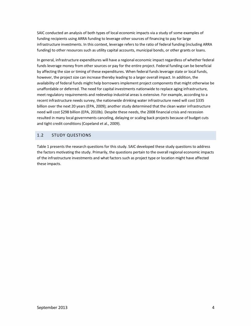
Table 1 presents the research questions for this study. SAIC developed these study questions to address the factors motivating the study. Primarily, the questions pertain to the overall regional economic impacts of the infrastructure investments and what factors such as project type or location might have affected these impacts.
September 2013 4

TAB LE 1. STUDY QUE STIONS AND C OR RE SPOND ING RE SE ARC H QUESTIONS
OVERARCHING STUDY QUESTIONS DETAILED RESEARCH QUESTIONS
What impact did the selected projects have on the local economies?
• What were the quantifiable direct, indirect and induced economic impacts of the State Revolving Fund (SRF) or other program project on the regional economy during the implementation phase (i.e., during the period when the project funds were expended)?
• What might the regional economic impacts of the project be during the post-project period?
• Do the quantitative impacts differ by technology or project type? How might technology affect the relative success or effectiveness of ARRA funding on local economic growth?
• Do the quantifiable economic impacts vary by location (e.g., region or urban versus rural)? How does location affect the relative success or effectiveness of ARRA funding on local economic growth?
• What kind of qualitative market and nonmarket impacts will the project have in the intermediate- and long-term (e.g., environmental- or health-related benefits)?
How do subsidy levels affect the extent of local impact?
• Do the quantitative impacts differ by subsidy level? • How might the level and/or type of subsidy affect the relative success or
effectiveness of ARRA funding in terms of the regional economic impact? How do leveraging levels affect the extent of local impact?
• Do the quantitative impacts differ by degree of leveraging? How might different leveraging schemes affect the relative success or effectiveness of ARRA funding on local economic growth? (e.g., Did the presence of additional local or state funds affect project type or project scope?)
September 2013 5

This page intentionally blank.
September 2013 6

SECTION 2. METHODOLOGY AND DATA SOURCES
2.1 STUDY DESIGN
The study has two parts. The first part is a qualitative analysis of anticipated future economic and environmental benefits, based on expert interviews as well as information in regulatory benefit studies. The second part is a regional economic impact analysis, which is a quantitative analysis of how the project expenditures – including the ARRA funding – affected total output in the local economy. Section 3.1 provides a summary of the case study results for the qualitative analysis while Section 3.2 provides the results for this quantitative analysis. The qualitative and quantitative analyses for each of the case studies are in the Appendices.
A regional economic impact analysis shows how expenditures for a project, such as constructing a new wastewater treatment plant, can have a greater impact on total local output because of a multiplier effect.1 This effect occurs because of linkages throughout the local economy–one industry’s cost is another industry’s revenue. Therefore, increased direct expenditures made by the industry implementing an ARRA-funded project lead to increased economic activity among its supplier industries and, in turn, their supplier industries. The increased supplier or ’upstream‘ economic activity is called indirect expenditures. The upstream economic activity includes wages to employees. When their expenditures stimulate the local economy, it is called induced expenditures. The total impact of a project is the sum of the direct, indirect and induced expenditures.
One widely used regional impact analysis model is the Regional Input-Output Modeling System (RIMS II) developed by the U.S. Bureau of Economic Analysis (BEA). For example, the Housing and Urban Development program used RIMS II multipliers to conduct a study of the regional economic impacts of ARRA-funded Public Housing Authority (PHA) projects.2
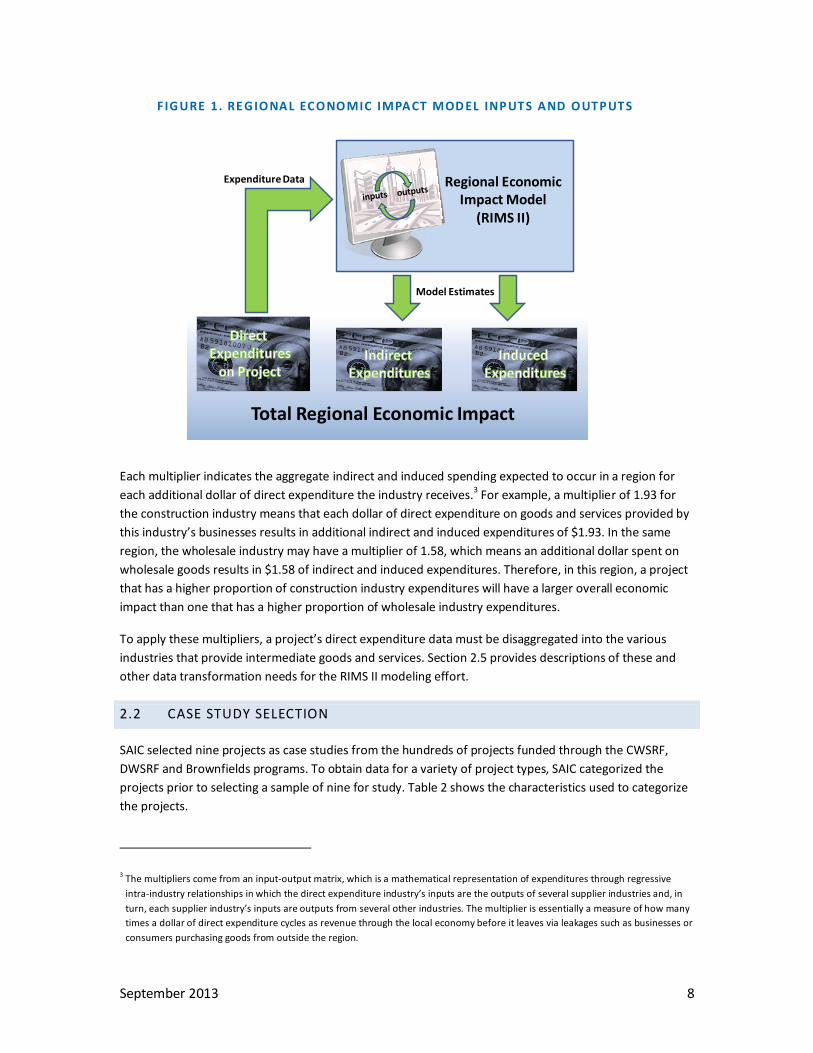
Figure 1 shows that the RIMS II model uses a project’s direct expenditures to generate estimates of indirect and induced expenditures. It generates these estimates using industry-level multipliers. RIMS II has multipliers for each of the 406 industries and these multipliers can vary by region. This variation comes from differences in regional industrial mix as well as differences in the input-output linkages among a region’s industries.
1 In essence, a regional economic impact analysis is a comparison of two alternative scenarios – the local economy without the project and the local economy with the project. The purpose of the comparison is to assess the net effect of the project in terms of growth in economic output. The method in this study uses a modeling approach that estimates the change or growth in the economy without having to estimate the level of economic output for both scenarios.
2 PHAs throughout the nation used $4 billion of ARRA funding to finance housing construction and renovation projects. A study of 20 PHAs that spent a total of $1.2 billion on capital investments, including $0.7 billion in ARRA funds that leveraged an additional $0.5 billion from other sources, estimated a total economic impact of almost $3.8 billion (Econsult Corporation, no date).
September 2013 7
F IGURE 1. RE GIONAL EC ONOMIC IMPACT MOD EL INPUTS AND OUTPUTS
Regional EconomicImpact Model
(RIMS II)
Total Regional Economic Impact
Expenditure Data
Model Estimates
September 2013 8
Each multiplier indicates the aggregate indirect and induced spending expected to occur in a region for each additional dollar of direct expenditure the industry receives.3 For example, a multiplier of 1.93 for the construction industry means that each dollar of direct expenditure on goods and services provided by this industry’s businesses results in additional indirect and induced expenditures of $1.93. In the same region, the wholesale industry may have a multiplier of 1.58, which means an additional dollar spent on wholesale goods results in $1.58 of indirect and induced expenditures. Therefore, in this region, a project that has a higher proportion of construction industry expenditures will have a larger overall economic impact than one that has a higher proportion of wholesale industry expenditures.
To apply these multipliers, a project’s direct expenditure data must be disaggregated into the various industries that provide intermediate goods and services. Section 2.5 provides descriptions of these and other data transformation needs for the RIMS II modeling effort.
2.2 CASE STUDY SELECTION
SAIC selected nine projects as case studies from the hundreds of projects funded through the CWSRF, DWSRF and Brownfields programs. To obtain data for a variety of project types, SAIC categorized the projects prior to selecting a sample of nine for study. Table 2 shows the characteristics used to categorize the projects.
3 The multipliers come from an input-output matrix, which is a mathematical representation of expenditures through regressive intra-industry relationships in which the direct expenditure industry’s inputs are the outputs of several supplier industries and, in turn, each supplier industry’s inputs are outputs from several other industries. The multiplier is essentially a measure of how many times a dollar of direct expenditure cycles as revenue through the local economy before it leaves via leakages such as businesses or consumers purchasing goods from outside the region.

TAB LE 2. CH ARAC TER IST IC S USE D TO CATEGOR IZE ARR A PR OJEC TS FOR CASE STUDY SELE CTION
CHARACTERISTIC VALUES REASON TO CONSIDER CHARACTERISTIC
Program CWSRF DWSRF Brownfields
Regional economic impacts and benefits will differ by type of program.
Project size Small (< $1 million) Medium ($1 to $10 million) Large (>$10 million)
Regional economic impacts will differ by project size.
Project type Varies by program The types of expenditures and hence the types of regional economic impacts will differ by project type.
Leverage - ratio A:B of federal funds (A) to non-federal funds (B) spent on a project)1
High leverage (> 3:1) Medium leverage (between 1:1 and 3:1) Low leverage (< 1:1)
Degree of leverage may affect post-project regional economic impacts because leveraged funding will presumably require repayment.
1 The federal funding in this ratio includes ARRA funds as well as other federal sources such as the federal portion of traditional SRF loans.
Table 3 provides a list of the selected case studies alon
g with their locations and brief project descriptions. Table 4 shows a summary of the case study programs, project sizes, project types and leverage intensities. There are four case studies from each of the SRF funding programs, which account for the vast majority of EPA’s ARRA funding, and one from the Brownfields program. The DWSRF and CWSRF project types come from the categories of projects most frequently funded (e.g., piping replacement/extensions and treatment). Finally, project sizes vary, as well as leverage amounts.
TAB LE 3. CASE STUDY PR OJEC T LOCATION AND DE SC R IPT ION
PROJECT NAME LOCATION PROJECT DESCRIPTION
Drinking Water State Revolving Fund Projects West End Drinking Water Reservoir
Hagerstown, Maryland
Partially replace 11 million gallon leaky, uncovered storage reservoir with 6.8 million gallon storage tank.
Amsterdam Drinking Water Treatment Plant Upgrades
Amsterdam, New York
Implement multiple equipment upgrades to existing conventional filtration plant to deal with drinking water violations for disinfection byproducts and lead.
Athens Drinking Water Distribution System Improvement
Athens, Ohio Replace frequently failing distribution main line and upgrade related pump and electrical system.
Pine Bluffs Meter Installation Pine Bluffs, Wyoming
Replace failing manual meters with radio signal meters, add meters to unmetered service lines, and move meter positions to connection with main line to enhance leak detection.
Clean Water State Revolving Fund Projects
Town of Cape Charles Wastewater Treatment Plant Upgrades
Cape Charles, Virginia
Retrofit existing wastewater treatment facility with advanced treatment to reduce nitrogen and phosphorus concentrations in discharge and also provide water suitable for nonpotable reuse (e.g., irrigation).
City of Hedrick Wastewater Treatment Plant Upgrades Hedrick, Iowa
Construct new treatment plant to reduce ammonia discharges to meet new permit limits, rehabilitate and increase lift station capacity to prevent overflows during storm events, and replace
September 2013 9

PROJECT NAME LOCATION PROJECT DESCRIPTION conventional sludge drying bed with a reed bed.
Grant County Sanitary District Extension
Sewer Grant County, Kentucky
Extend sewer service lines to new areas including a campground with an aging treatment plant and a mobile home park with a failing treatment plant.
Santa Cruz County Reduction Santa Cruz Implement roadside integrated vegetation management plan to of Nonpoint Source Sediment County, reduce pesticide application, mowing and presence of invasive and Pesticide Pollution California species.
Brownfields Project
St. Paul Port Authority Beacon Bluff Assessment and Cleanup
St. Paul, Minnesota
Conduct site assessment and cleanup activities for former 3M production facilities and surrounding acreage and install ’Next Generation‘ regional stormwater infiltration basin to treat runoff from neighboring areas.
TAB LE 4. CASE STUDY PR OJECTS BY PROGR AM AND SE LEC TION C ATEGO RY
Drinking Water State Revolving Fund Projects
PROJECT NAME
West End Drinking Water Reservoir
PROJECT TYPE CATEGORY
Storage
PROJECT SIZE CATEGORY
Medium
LEVERAGE CATEGORY
High
Amsterdam Drinking Water Treatment Plant Upgrades
Treatment Large High
Athens Drinking Water Distribution System Improvement
Piping Small High
Pine Bluffs Meter Installation Metering Medium High
Clean Water State Revolving Fund Projects Town of Cape Charles Wastewater Treatment Plant Upgrades Treatment Large Low
City of Hedrick Wastewater Treatment Plant Upgrades
Treatment Medium Medium
Grant County Sanitary Sewer District Extension Piping Medium Medium
Santa Cruz County Reduction of Nonpoint Source Sediment and Pesticide Pollution
Stormwater Small Low
Brownfields Project St. Paul Port Authority Beacon Bluff Assessment and Cleanup Redevelopment Medium Medium
2.3 CASE STUDY DATA COLLECTION
The analysis method required data from a variety of sources. Table 5 provides an overview of the data needs and sources. For each case study, SAIC obtained an expenditure breakdown that could be used to disaggregate total project expenditures by the industries used to categorize the expenditures within RIMS II. SAIC also obtained information to identify the local region for economic impact analysis. The region included the county where the project was implemented and any surrounding counties that were major suppliers of materials and labor. The Bureau of Economic Analysis developed custom RIMS II multipliers for each of the nine project regions. SAIC also interviewed one expert per case study to learn more about
September 2013 10

the current and future impacts of the project on environmental quality and the local economy. Usually this was a design engineer or utility official who understood the infrastructure needs that motivated the project. Finally, to identify potential environmental benefits, SAIC consulted regulatory technical support documents such as economic impact analyses for drinking water rules.
TAB LE 5. DATA REQUIRE ME NTS AND SOURCE S
TYPES OF REQUIRED DATA DATA SOURCES
Project expenditure breakdown Borrowers or finance documents, building contractors and RIMS II industry list
RIMS II multipliers for local region Bureau of Economic Analysis
Expert opinion Local utility or engineering experts
National environmental benefits information EPA national regulatory technical support documents
2.4 QUALITATIVE ANALYSIS – ENVIRONMENTAL AND HEALTH RISK REDUCTION BENEFITS
For the qualitative discussion of environmental and health risk reduction benefits, SAIC obtained information from relevant regulatory analysis documents. These documents contained inventories of the types of benefits that EPA attributes to actions taken to implement a particular rule. For example, the Amsterdam, New York water treatment plant upgrades reduced levels of disinfection byproducts and lead throughout its distribution system. Reducing the exposure to regulated disinfection byproducts can reduce the risk of bladder, colon and rectal cancers, and also reduce the risk of reproductive and developmental effects (EPA, 2006). In addition, improving corrosion control that reduces lead levels in households that have lead service lines and plumbing can reduce risks of damage to the brain and kidneys, and interference with the production of red blood cells that carry oxygen, especially among infants, children and pregnant women (EPA, 2007). In addition to health risk reductions, the upgrades may improve customer relations because the utility no longer has to notify its customers of health standard violations.
Some case study projects do not have a direct link to a recent federal regulation. For example, many projects are expenditures to replace aging and failing infrastructure such as water distribution pipes or sewer collection mains. SAIC collected data for the qualitative benefits of these projects via expert interview and literature review to identify the types of benefits that can be associated with these projects. For example, replacement of aging drinking water pipes can have benefits associated with health risk reduction (e.g., reducing infiltration of contaminated water into service lines) as well as improved water delivery services (e.g., reduced risk of catastrophic pipe failure, temporary loss of water supply and risk of flooding in low-lying areas).
September 2013 11

2.5 QUANTITATIVE ANALYSIS – REGIONAL ECONOMIC IMPACT MODELING
As a first step in the quantitative analysis, SAIC transformed the case study expenditure data into quantities that match the data input requirements for a RIMS II modeling effort (BEA, 2012; BEA, 1997). This required disaggregating expenditures into material purchases (i.e., revenues to supplier industries), labor expenses (only those paid as direct expenditures in the primary industry; labor expenses incurred by upstream industries remain in those industry totals because the supplier industry multipliers take induced spending into account), and transportation expenses (these represent revenues to the transportation industry).
In addition, SAIC identified the share of the direct expenditures that accrued to suppliers and businesses located in the region. RIMS II framework presumes that the share accruing to non-regional sources represents ’leakage,’ i.e., dollars that leave the local region and therefore provide no additional indirect or induced local economic benefit. For example, a water treatment project that includes a $1 million skid-mounted membrane filter purchased from a vendor in another state will result in less regional economic growth than a project that includes a $1 million sand filter built using locally sourced materials and services such as excavation and concrete basin forming and pouring for the filter basin.
SAIC applied the region-specific RIMS II multipliers to the local expenditures using the recommended “bill-of-goods” method (BEA, 2012; BEA, 1997). This method required that direct expenditures be disaggregated by supplier industry category.
Table 6 shows an example analysis for Santa Cruz County, California. It shows that after allocating each expenditure line item to an industry in RIMS II, there are two industries that received revenues for providing inputs to the project (construction and professional and technical services). In addition, direct expenditures were paid as wages for Santa Cruz County employees who worked on the project; RIMS II also has a “households” multiplier for this category of direct expenditure. The multipliers range from 0.88 for households to 1.62 for both construction and professional and technical services. According to the multipliers for the local region, the direct expenditures of approximately $0.84 million resulted in an additional $1.17 million of indirect and induced expenditures in the county. The total economic impact of direct, indirect and induced expenditures was approximately $2.0 million ($0.84 million + $1.17 million). The impact ratio is approximately 2.4 ($2.0 million divided by $0.84 million).
September 2013 12

TAB LE 6. E XAMPLE OF MULTIPL IER ANALYSIS INPUTS AND OUTPUTS ( SANTA C RUZ COUNTY )
INDUSTRIAL SECTOR
Construction
DIRECT IMPACTS
$16,225
RIMS II MULTIPLIER1
1.62
INDIRECT AND INDUCED IMPACTS
$26,349
Professional and Technical Services $570,475 1.62
$921,371
Households $253,000 0.88 $222,387
Indirect and Induced Impacts $1,170,107
Add Total Project Value $839,700
Total Output Impact $2,009,807 1 These are Type II multipliers, which means the multipliers for the construction and professional and technical services industries include indirect expenditures for the intermediate goods used by these industries as well as induced expenditures for all associated labor expenses. The multiplier that applies to direct expenditures in the households category (i.e., incomes earned by the Santa Cruz County employees) includes indirect household purchases of local goods and services as well as induced expenditures of wages earned by employees of those local businesses.
2.6 STUDY LIMITATIONS
As with any study, there are some limitations to the findings based on available data, resource and time constraints and statutory limitations (specifically, the Paperwork Reduction Act). These conditions can cause estimation difficulties, uncertainties and biases, arising from a number of factors, including those described below:
• The limited number of case studies restricts the extent to which regional economic impact results can be generalized. The distribution of expenditures and regional multipliers are unique to each project and, therefore, the regional economic impacts vary by project.
• The regional economic impacts of projects implemented in the 2009 to 2011 timeframe may not be typical of such investments because the underlying conditions (e.g., relatively tight credit markets and high unemployment) are not typical. Thus, the degree of ARRA leverage among the funded projects may be higher than under more typical economic circumstances.
• SAIC’s ability to disaggregate case study expenditures by industry affects the reliability of the RIMS II multiplier analysis. Some expenditure data were more detailed and, therefore, more readily allocated. In some cases, SAIC needed to estimate material and labor shares of direct expenditures.
• The discussion of qualitative environmental benefits, including health risk reductions, reflects the types of benefits expected to occur nationwide as a result of meeting a regulatory standard. The benefits realized in the region affected by a particular project might not include all of the types of benefits identified.
September 2013 13

This page intentionally blank.
September 2013 14

SECTION 3. FINDINGS
This section contains two subsections of study results – qualitative economic and environmental impacts and quantitative regional economic impact modeling results. Table 7 below summarizes the big picture findings for each study question. The big picture findings are based on information gathered from interviews with project recipient staff (local utility and engineers) for the qualitative impacts and analysis of modeling results (for the quantitative results). The sections of the report following Table 7 include a thorough discussion of the findings.
TAB LE 7. STUDY QUE STIONS WITH B IG P IC TUR E F IND INGS
OVERARCHING STUDY QUESTION – LOCAL ECONOMIC IMPACTS
What impact did the selected projects have on the local economies?
DETAILED RESEARCH QUESTIONS BIG PICTURE FINDINGS Quantifiable project impacts. What were the quantifiable direct, indirect and induced economic impacts of the SRF or other program project on the regional economy during the implementation phase (i.e., during the period when the project funds were expended)?
Identifiable longer-term economic impacts. What might the regional economic impacts of the project be during the post-project period?
Impact variability by project type. Do the quantitative impacts differ by technology or project type? How might technology affect the relative success or effectiveness of ARRA funding on local economic growth?
Impact variability by location. Do the quantifiable economic impacts vary by location (e.g., region or urban versus rural)? How does location affect the relative success or effectiveness of ARRA funding on local economic growth?
Identifiable qualitative impacts. What kind of qualitative market and nonmarket impacts will the project have in the intermediate- and long-term (e.g., environmental- or health-related benefits)?
The quantifiable impacts were greater than the expenditures. The quantifiable regional economic impact per dollar of project expenditure ranges from $1.58 to $2.96 across the nine case study projects.
There are a variety of post-construction regional economic impacts. They include cost savings for utilities and customers of reduced water use and/or energy production costs and enhanced capacity for residential and commercial growth because of increased water and wastewater utility capacity.
Project type affected local expenditure share, which affected overall impact. The projects that retained the highest proportion of direct expenditures in the local community generally have higher impact ratios. For example, treatment plant upgrades required outside expenditures on treatment equipment, which reduced regional economic impacts.
Location affects the magnitude of impact. The rural regions tended to have lower industry and households multipliers, which reduced the overall impact of local expenditures.
All projects had multiple qualitative impacts. Most of the projects had identifiable health risk reductions or environmental benefits in addition to long-term cost savings.
September 2013 15

OVERARCHING STUDY QUESTION – EFFECT OF SUBSIDY
How do subsidy levels affect the extent of local impact?
DETAILED RESEARCH QUESTIONS BIG PICTURE FINDINGS Effect of subsidy level on economic impact. Do the quantitative impacts differ by subsidy level? How might the level and/or type of subsidy affect the relative success or effectiveness of ARRA funding in terms of the regional economic impact?
ARRA subsidy was a key financial feature. For five of the projects, all of the ARRA funding was subsidized and for a sixth the ARRA funding was a grant. These six projects will benefit in the future from lower future capital financing costs. Some of the projects that were highly leveraged by subsidized ARRA funds would not have proceeded without the funding.
OVERARCHING STUDY QUESTION – EFFECT OF LEVERAGE
How do leveraging levels affect the extent of local impact?
DETAILED RESEARCH QUESTIONS BIG PICTURE FINDINGS Effect of leverage on economic impact. Do the quantitative impacts differ by degree of leveraging? How might different leveraging schemes affect the relative success or effectiveness of ARRA funding on local economic growth? (e.g., Did the presence of additional local or state funds affect project type or project scope?)
Degree of leverage may have increased level of economic impact. More highly leveraged projects generally had higher regional economic impacts, although not always. There is not enough variation in the small sample to assess the relative success of different leveraging schemes. Most of the projects - regardless of type - relied heavily on federal resources including ARRA funding.
3.1 RESULTS OF QUALITATIVE ECONOMIC AND ENVIRONMENTAL IMPACT REVIEW
The case study projects were implemented to meet a variety of infrastructure objectives. Consequently, they will provide a wide variety of mid-term and long-term economic and environmental benefits, ranging from health risk reductions to surface water quality improvements to economic growth support. Table 8 provides a list of common benefit categories and identifies which projects will provide each benefit. It also shows that each project provides multiple benefits. The Appendices provide detailed discussion of the benefits for each case study.
September 2013 16

TAB LE 8. MED IUM- AND LONG-TER M BE NE FITS OF PR OJE C T
BENEFIT
HUMAN HEALTH RISK REDUC
TION
IMPROVE SURFACE WATER QUALITY-NUTRIENTS/ SEDIMENTS
IMPROVE SURFACE WATER QUALITY-TOXIC
REDUCTION
WATER SAVING
REUSE
ENERGY SAVI
NGS
SUPPORTS LOCAL GROWTH OBJECTI
UTILITY AND/OR COMMERCIAL COST SAVINGS
September 2013 17
Drinking Water State Revolving Fund Projects West End (Hagerstown, Maryland) √ √ √ √
Amsterdam (New York) √ √ √ √ √
Athens (Ohio) √ √ √ √
Pine Bluffs (Wyoming) √ √ √ √
Clean Water State Revolving Fund Projects Cape Charles (Virginia) √ √ √ √
Hedrick (Iowa) √ √
Grant County (Kentucky) √ √
Santa Cruz County (California) √ √
Brownfields Project St. Paul (Minnesota) √ √ √
All of the DWSRF projects will reduce water use and production costs such as energy costs. The non-metering projects will also reduce health risks. The Amsterdam project reduces health risks by improving the quality of the water distributed to customers, while the West End and Athens projects help maintain water quality in the distribution system. The West End project provided covered water storage, which prevents drinking water contamination that might occur in an uncovered storage reservoir. The Athens project replaced underground distribution piping that regularly failed, which prompted boil alerts to ensure drinking water safety. Although the Pine Bluffs project helped identify leaking pipes, the health benefits, if any, are probably minor compared to the reductions in water loss.
The four CWSRF projects will improve surface water quality by reducing the discharge of nutrients, sediments or toxic substances to surface waters. The St. Paul redevelopment project similarly improves surface water quality by reducing sediments in stormwater runoff. It will also improve groundwater quality by removing contaminated soils from the site and by improving stormwater infiltration treatment via the ’Next Generation‘ infiltration basin.
Although most of the projects have economic benefits in the form of reduced future utility costs, four projects explicitly support community economic growth objectives. Two of the treatment projects (Amsterdam and Cape Charles) increased utility capacity, which will support long-term residential and commercial growth. Both also indirectly benefit commercial customers. Amsterdam’s improvements in water quality benefit a local manufacturer of baby food. Cape Charles’ new capacity for water reuse will benefit entities that can use nonpotable water for irrigation such as golf courses. By reducing water loss, the Pine Bluffs project helps extend water supply and provides capacity for growth.

The St. Paul Port Authority redevelopment project provides competitively priced development property that is centrally located in the urban core.
3.2 RESULTS OF QUANTITATIVE REGIONAL ECONOMIC IMPACT MODELING
The case studies encompass a wide range of financial conditions. Project size varies substantially – from less than $1 million to almost $19 million (see Table 9). Similarly, the ARRA funding proportion ranges widely from 16% (Grant County) to 90% (Pine Bluffs). Finally, financing conditions range from highly leveraged (i.e., a ratio of ARRA and other SRF funding to other funding of more than 10:1) to very low leverage (i.e., a ratio of less than 0.4:1).
Almost all of the ARRA funds are fully subsidized via principal forgiveness. This type of subsidy will continue to benefit the local economies following the infrastructure investment. The ARRA funds that have the principal forgiveness subsidy do not have to be repaid to either the SRFs or the federal government. Normally, a utility that borrows funds for infrastructure investments would raise customer water or wastewater rates to repay the borrowed funds. Furthermore, repayments made to state or federal agencies immediately leave the local economy. Therefore, principal forgiveness subsidies will reduce the amount of future rate increases and help keep money in the local economy.
TAB LE 9. CASE STUDY F INANC IAL DATA ( $ IN MILL IONS)
PROJECT NAME TOTAL
PROJECT FUNDING
ARRA FUNDING
ARRA SUBSIDY1
LEVERAGE RATIO2
West End Drinking Water Reservoir $6.64 $5.31 $0 6.3:1
Amsterdam Drinking Water Treatment Plant Upgrades $10.65 $5.08 $5.08 132:1
Athens Drinking Water Distribution System Improvement $0.88 $0.32 $0.32 10.7:1
Pine Bluffs Meter Installation $1.11 $1.00 $0.76 9.5:1
Town of Cape Charles Wastewater Treatment Plant Upgrades $18.90 $6.08 $6.08 0.5:1
City of Hedrick Wastewater Treatment Plant Upgrades $4.29 $0.90 $0.90 2.6:1
Grant County Sanitary Sewer District Extension $1.93 $0.30 $0.16 1.1:1
Santa Cruz County Reduction of Nonpoint Source Sediment and Pesticide Pollution
$0.84 $0.23 $0.23 0.4:1
St. Paul Port Authority Beacon Bluff Assessment and Cleanup $2.59 $1.40 $1.40 1.6:1
Source: DWSRF, CWSRF and Brownfields databases. 1 Subsidy amount shown is principal forgiveness except for the St. Paul Port Authority funding, which is a Brownfields grant. The West End project financing did not include any principal forgiveness; the ARRA funding is a 30-year loan with a 0% interest rate. 2 The leverage ratio shows the ratio of all federal funding to other resources. Several case studies received non-ARRA federal funding.
September 2013 18

3.2.1 VARIATIONS IN LOCAL EXPENDITURES
Table 10 shows the total expenditures for which line-item details were available and the portion determined to accrue to local businesses and employees.4 The proportion of local spending suggests a major difference in local spending patterns across project types. For five of the case studies, local expenditures exceed 90% of enumerated expenditures. This outcome is not surprising given the nature of these projects, which use materials and construction activities that can be locally provided in many areas (e.g., laying pipe or roadside maintenance). In some cases, even though the project occurs in a rural county, the local area includes a nearby major urban area that provides materials and skilled workers. For example, the Cape Charles project occurred in one of Virginia’s Eastern Shore counties, but most of the labor and materials came from the Virginia Beach-Norfolk-Newport News metropolitan area.
The three treatment projects and the metering project, however, have substantially lower local expenditure shares – 39 to 66 percent, compared to 94 to 100 percent for the five other projects. The difference can be attributed to relatively large purchases of specialized treatment or meter installation equipment from vendors located outside the local area. Consequently, ARRA funding for projects requiring equipment sold by only a few U.S. manufacturers is likely to have had a lower local economic impact because a larger portion of direct expenditures - and the resulting indirect and induced expenditures - accrue elsewhere.
TAB LE 10. CASE STUDY PROJE CT TY PE AND LOC AL E XPE ND ITURE S ($ IN MILL IONS)
PROJECT NAME PROJECT TYPE CATEGORY
TOTAL EXPENDITURES1
LOCAL EXPENDITURES $ %
St. Paul Port Authority Beacon Bluff Assessment and Cleanup
Redevelopment $1.60 $1.60 100%
Santa Cruz County Reduction of Nonpoint Source Sediment and Pesticide Pollution Stormwater $0.84 $0.84 100%
Athens Drinking Water Distribution System Improvement
Piping $0.82 $0.82 100%
West End Drinking Water Reservoir Storage $5.22 $5.12 98%
Grant County Sanitary Sewer District Extension Piping $1.93 $1.82 94%
Town of Cape Charles Wastewater Treatment Plant Upgrades Treatment $15.16 $9.97 66%
Amsterdam Drinking Water Treatment Plant Upgrades
Treatment $10.65 $6.74 63%
City of Hedrick Wastewater Treatment Plant Upgrades Treatment $3.36 $2.12 63%
Pine Bluffs Meter Installation Metering $0.97 $0.38 39% 1 Expenditures for which industry detail was available, which may represent a portion of overall project expenditures reported in Table 9. The quantitative analysis cannot include expenditures for which industry detail is not available.
September 2013 19
4 The total based on available expenditure data is sometimes less than the total project cost (shown as Total Project Funding in Table 9. Case Study Project Data ($ in Millions)) because SAIC did not receive expenditure details for all project costs. The quantitative analysis is based on the available expenditure data because the distribution of missing expenditures across industries or between local and nonlocal categories is not known.

The distribution of local expenditures across industries also varies across the projects. Figure 2 shows local expenditures broken into the percent accruing to the following major groups:
• Production industries (e.g., construction and manufacturing).
• Trade and transportation industries.
• Service industries (e.g., professional and technical services).
• Households.
This breakdown shows that two projects had expenditures dominated by service industries: the Santa Cruz County vegetation management project and the St. Paul Brownfields redevelopment project. Industry expenditures for the other projects tended to be dominated by production industries and trade and transportation industries.
Direct expenditures paid to households ranged from none for the St. Paul project to almost 45% for the Amsterdam project. The St. Paul project expenditures did not include any St. Paul Port Authority labor expenses; all funds were expended on contracted services for site assessment and cleanup. The household expenditures for the Amsterdam project comprise labor expenditures for treatment plant construction activities. As the next section shows, direct expenditures to households tended to decrease the total economic impact of a project because household expenditures can introduce a lot of leakage to a local economy. Consequently, the ability to disaggregate construction-related expenditures into material and labor expenditures is an important factor that affects the accuracy of the impact estimate.
September 2013 20

F IGURE 2. D ISTR IBUTION OF LOC AL E XPE ND ITURE S BY MAJOR IND USTRY GROUP
0.0%
10.0%
20.0%
30.0%
40.0%
50.0%
60.0%
70.0%
80.0%
90.0%
100.0%
Perc
ent o
f Loc
al E
xpen
ditu
res
Production Industries Trade/Transportation Service Industries Households
3.2.2 VARIATIONS IN RIMS II MODELING RESULTS
Table 11 provides the RIMS II industry-level multipliers by region for the industries occurring most frequently across the case studies. These are the multipliers that SAIC applied to the industry-level expenditures to estimate indirect and induced economic impacts. Detailed information on the expenditure distributions by industry for each project is in the Appendices.
Within a region, the RIMS II multipliers in Table 10 vary across industries. In general, the industry multipliers within a study region are often closely grouped within a range of ± 0.2. This is true of the service industries as well as the production industries such as mining, utilities, construction and manufacturing (except for the Pine Bluffs and Athens projects). The consistent outlier across case studies is the multiplier for household expenditures. This multiplier applies to direct expenditures identified as labor expenditures. Factors that reduce the household expenditure multiplier include taxes and savings as well as purchases of consumer goods that are imported to the region from elsewhere. Because there is little variability across industries, but substantial variability between all industries and households, the proportion of direct expenditures allocated to the households category tends to have a large effect on the overall economic impact of a project. Therefore, a higher proportion of funding going directly to recipient labor expenses will decrease regional economic impacts.
September 2013 21

TAB LE 11. VAR IATIONS IN IND USTRY- LEVE L R IMS I I MULTIPL IER S
ULTUR MAN WHO TRANSP PROFESS ADMINIAL, UFAC LESAL ORTATIO IONAL & STRATIV FISHIN TURIN E N & E & MINI CONS HOUS
TECHNICINDUSTRY G, G TRAD WASTE NG TRUC EHOL
& E WAREH AL SERVICETION DS HUNTI OUSING SERVICE S
NG S West End 1.60 1.69 1.93 1.74 1.58 1.82 1.66 1.69 0.95
Amsterdam -- -- 1.87 1.68 1.65 1.83 1.78 -- 0.96
Athens -- -- -- 1.59 0.14 1.35 1.46 1.44 0.73
Pine Bluffs -- -- -- 1.76 0.95 1.52 1.84 -- 0.88
Cape Charles 1.57 1.72 1.92 1.67 1.72 1.97 1.88 -- 1.09
Hedrick 1.50 1.62 1.77 1.61 1.54 1.74 1.61 -- 0.88
Grant County 1.71 1.87 1.73 1.64 1.89 -- -- 1.02
Santa Cruz County -- -- 1.62 -- -- -- 1.62 -- 0.88
St. Paul -- -- 2.01 -- -- -- 1.99 1.86 --
Source: RIMS II industry-level multipliers from BEA. The Appendices contain multipliers for additional industries that were affected in only one or two case studies. ‘--' = no local direct expenditures tabulated for this industry so the multiplier is excluded from the analysis.
Within an industry, the variation of multipliers across the case study regions is relatively small with the exception of the multipliers for the Athens Ohio project. The relatively low industry-level multipliers for this region indicate that direct expenditures with local businesses tend to leak rapidly out of the local region compared to the other regions. This is especially true of expenditures in the manufacturing industry with a multiplier of 0.14, which indicates that most of the inputs for this industry come from business located outside the local region.
Table 12 shows a summary of the RIMS II modeling results. It contains the local portion of direct expenditures for each project and the estimates of indirect and induced expenditures from the RIMS II model. It also shows project-specific multipliers that SAIC calculated by dividing the total indirect and induced expenditure by the local direct expenditures for each project. The project-specific multiplier shows the average impact of a dollar of local direct expenditure, given each project’s unique distribution of expenditures across local industries. Thus, it is an expenditure-weighted average of the RIMS II industry-level multipliers for a given region (i.e., the multipliers in Table 11).
AGRIC
September 2013 22

TAB LE 12. D IRE CT E XPE ND ITURE S AND SUB SE QUE NT IND IREC T AND INDUCE D E XPE ND ITURE S ( $ IN MILL IONS)
PROJECT NAME LOCAL DIRECT EXPENDITURES (A)
INDIRECT AND INDUCED
EXPENDITURES (B)
PROJECT-SPECIFIC MULTIPLIER 1
(B)/(A) West End Drinking Water Reservoir $5.12 $8.37 1.63
Amsterdam Drinking Water Treatment Plant Upgrades
$6.74 $9.24 1.37
Athens Drinking Water Distribution System Improvement $0.82 $0.55 0.67
Pine Bluffs Meter Installation $0.38 $0.56 1.49
Town of Cape Charles Wastewater Treatment Plant Upgrades
$9.97 $14.68 1.47
City of Hedrick Wastewater Treatment Plant Upgrades $2.12 $2.98 1.41
Grant County Sanitary Sewer District Extension $1.82 $2.91 1.60
Santa Cruz County Reduction of Nonpoint Source Sediment and Pesticide Pollution
$0.84 $1.17 1.39
St. Paul Port Authority Beacon Bluff Assessment and Cleanup
$1.60 $3.14 1.96
1 These are not the industry-level RIMS II multipliers. They are weighted averages across the industries that experienced increased demand because of the project expenditures. Ratios shown may vary from detail because of independent rounding.
September 2013 23
The project-specific multipliers in Table 12 show a wide range of local economic interdependencies. At the low end, the value of 0.67 for the Athens project indicates that a $1 of incremental direct expenditures led to only $0.67 of additional indirect and induced expenditures. For this region, all direct expenditures accrued to businesses in two rural counties. SAIC retained this as a definition for the local area to evaluate an example of multipliers for highly localized direct expenditures in rural areas.
At the opposite end of the spectrum is the multiplier of 1.96 for the St. Paul Port Authority project. This high value reflects a region that can produce much of the supply chain needed for the funded project. The outcome may be typical of expenditures in a large urban area.
One result to note is that the project-specific multipliers in Table 12 tend to be smaller than the construction industry multipliers in Table 11. For example, the project-specific multiplier for the Pine Bluffs project is 1.49, which is lower than the region’s construction industry multiplier of 1.76. If SAIC had not used the bill-of-goods method shown above in Table 6 to estimate the regional economic impact and had simply applied the construction industry multiplier to the local expenditures for the infrastructure projects, the RIMS II output would generate higher impact estimates, which would have overstated the impact of expenditure pattern for this particular project. This result illustrates the importance of using a bill-of-goods approach.
Table 13 shows the combined effect of local expenditure shares and the regional multipliers. The estimates of total project impact are the sum of the indirect and induced expenditures shown in Table 12 and the total project expenditures (from Table 10). The final column shows the impact ratio, which is the

ratio of total project economic impact to total project expenditures. These ratios demonstrate that the case study project expenditures unambiguously achieved the objective of stimulating local economies during the recession.
TAB LE 13. TOTAL PROJE CT IMPAC T R ATIOS ( $ IN MILL IONS)
PROJECT NAME TOTAL PROJECT IMPACT (A)1
TOTAL EXPENDITURES2
(B) IMPACT RATIO3
(A) / (B) West End Drinking Water Reservoir $13.59 $5.22 2.60
Amsterdam Drinking Water Treatment Plant Upgrades
$19.89 $10.65 1.87
Athens Drinking Water Distribution System Improvement
$1.38 $0.82 1.67
Pine Bluffs Meter Installation $1.53 $0.97 1.58
Town of Cape Charles Wastewater Treatment Plant Upgrades
$29.84 $15.16 1.97
City of Hedrick Wastewater Treatment Plant Upgrades $6.34 $3.36 1.89
Grant County Sanitary Sewer District Extension $4.85 $1.93 2.51
Santa Cruz County Reduction of Nonpoint Source Sediment and Pesticide Pollution
$2.01 $0.84 2.39
St. Paul Port Authority Beacon Bluff Assessment and Cleanup $4.74 $1.60 2.96
1 Total Project Impact equals the sum of Total Expenditures and Indirect and Induced Expenditures. 2 Expenditures for which industry detail was available, which may represent a portion of overall project expenditures reported in Table 9. The quantitative analysis cannot include expenditures for which industry detail is not available. 3 Ratios shown may vary from detail because of independent rounding.
Figure 3 shows the impact ratios along with three other project dimensions. The y-axis contains the scale for the impact ratio, while the x-axis contains the scale for the ARRA proportion of total funding. The size of the bubbles and data labels indicate overall project size, while the bubble color indicates project type - blue for treatment projects, red for piping and storage projects, green for land use (vegetation and redevelopment) projects and orange for the metering project.
September 2013 24

F IGURE 3. IMPACT RATIOS BY AR RA FUND ING SH ARE , PROJE CT SIZE , AND PROJE CT TYPE
$6.64
$10.65
$0.88 $1.11
$18.90
$4.29
$1.93 $0.84
$2.59
1.50
1.70
1.90
2.10
2.30
2.50
2.70
2.90
3.10
3.30
0% 20% 40% 60% 80% 100% 120%
Impa
ct R
atio
ARRA Funding Share (%)
September 2013 25
Piping and land use projects (red and green bubbles) tend to
outperform treatment and metering projects (blue and orange bubbles).
This display format shows that, of the nine case studies included in the study, the smaller piping and land use (vegetation or redevelopment) projects (red and green bubbles) tend to have higher impact ratios, regardless of the wide variations in ARRA funding shares; the one exception is the Athens project ($0.88), which has the second lowest impact ratio. In contrast, the treatment plant projects (blue bubbles) have ARRA funding shares in a narrower 20-to-50 percent range and had consistently lower impact ratios than four of the piping and landscape projects. The metering project had a high ARRA funding share, but a low impact ratio.
Figure 4 shows the same impact ratio and project type and size dimensions, but the x-axis now shows the proportion of project direct expenditures spent in the local area. There are three distinct categories of results.
First, there are four projects that have high local spending shares and impact ratios above 2.3. These projects have aggregate multipliers in Table 12 that are in the 1.39 to 1.96 range, but the high local expenditure share boosts the impact ratio above 2.30. The second category has one project with a high local expenditure share, but an impact ratio well below 2.00. This is the Athens project, which has a very low aggregate multiplier, as noted above.

F IGURE 4. IMPACT RATIOS BY LOC AL D IRE CT E XPE ND ITURE PR OPORTION, PROJEC T SIZE AND PR OJEC T TY PE
$6.64
$10.65
$0.88 $1.11
$18.90
$4.29
$1.93 $0.84
$2.59
1.50
1.70
1.90
2.10
2.30
2.50
2.70
2.90
3.10
3.30
0% 20% 40% 60% 80% 100% 120%
Impa
ct R
atio
Local Direct Expenditure Proportion (%)
September 2013 26
Piping and land use projects (red and green bubbles) tend to boost local economies more than treatment and metering projects (blue and orange bubbles).
The third category includes the projects with local expenditure proportions below 80%. Despite having aggregate multipliers in the 1.37 to 1.47 range, the impact ratios for the three treatment projects are below 2.30 because of the low local expenditure shares. The metering project has a slightly higher aggregate multiplier (1.49), but a smaller impact ratio because of the low local expenditure proportion.
Table 14 shows a summary of the case studies grouped by impact ratio and local expenditure share. This table suggests that in the nine case studies included in this study, the impact ratio is highly correlated with local expenditure share. The exception, however, is the Athens case study. None of the case studies were in the fourth category: high impact ratio and low local expenditure share. This outcome is theoretically possible, however. For example, the St. Paul case study has a high enough weighted average industry multiplier (1.97) that the project impact ratio would exceed 2.30 even if the local expenditure share were as low as 67%. Nevertheless, the results point to the importance of keeping a high proportion of direct expenditures in the local economy to achieve a high overall impact.

TAB LE 14. CASE STUDY D ISTR IB UTION BY IMPACT RATIO AND LOCAL E XPEND IT UR E SH ARE
HIGHER IMPACT RATIO (>2.3) LOWER IMPACT RATIO (<2.3)
West End
HIGHER LOCAL EXPENDITURE SHARE (≥90%)
Grant County Santa Cruz County
Athens
St. Paul
no case study
Amsterdam Pine Bluffs Cape Charles Hedrick
LOWER LOCAL EXPENDITURE SHARE (<90%)
3.2.3 VARIATIONS IN FUNDING LEVERAGE
This section returns to the concept of how leveraging resources helped local economies during the recession. To quantify the degree to which a project used federal funding to leverage other resources, SAIC calculated a ratio of federal funding (ARRA funding and other federal sources) to local resources funding the project. A higher leverage ratio means that more resources for the project are coming from outside the local area in the form of ARRA funds or other SRF funds. A lower leverage ratio means that the recipient has other financial resources such as annual maintenance funds for pipe replacement.
There are three observations to make about leverage based on the case study information. First, higher leverage generally led to higher regional economic impacts. Figure 5 illustrates this outcome. The figure shows four data dimensions for each case study: leverage ratio (shown on the x-axis), total economic impact (shown on the y-axis), project size (bubble size reflects dollar value), and project type (bubble color). For six of the nine projects, larger leverage ratios and higher total economic impacts are positively correlated. These six projects include three types: two treatment projects (blue bubbles), two piping and storage projects (red bubbles), and both land use projects (green bubbles).
There are three outliers. The first is a large $18.9 million treatment project that was not highly leveraged, but had a larger economic impact than other projects with the same degree of leverage. The other two are the small $0.88 million piping project and the $1.11 million metering project that were more highly leveraged than the other projects that had economic impacts of similar sizes.
September 2013 27

F IGURE 5. TOTAL EC ONOMIC IMPACT BY LEV ER AGE RATIOS, PROJEC T SIZE AND PR OJEC T TY PE
$6.64
$10.65
$0.88 $1.11
$18.90
$4.29
$1.93 $0.84 $2.59
$0.00
$5.00
$10.00
$15.00
$20.00
$25.00
$30.00
$35.00
0.1 1.0 10.0 100.0 1000.0
Tota
l Eco
nom
ic Im
pact
($ m
illio
ns)
Leverage Ratio (log scale)
September 2013 28
The second observation comes from an unusual ARRA funding condition. Usually, high leverage has a disadvantage of creating high indebtedness, which can increase future debt-servicing costs. For most of these projects, however, the ARRA funding was subsidized by principal forgiveness. This condition means that some portion of the loan principal does not need to be repaid. For five of the projects, all of the ARRA funding was subsidized; for a sixth project, the ARRA funding was a grant, which has the same effect as principal forgiveness. Thus, the presence of principal forgiveness results in the opposite outcome – more highly leveraged projects benefit from lower future capital financing costs.
The third observation is that the ability to leverage local resources with federal funding was either an important catalyst in moving projects forward during the recession or a major contributor to the project existing at all. For example, ARRA funding and additional SRF funding accounted for almost all the cost of the Amsterdam treatment plant and more than 70% of the Hedrick treatment plant cost. These cities might have had to choose different regulatory compliance strategies if they had to rely solely on local financing. The Santa Cruz County Integrated Vegetation Management project was placed on hold because the recession depleted the expected funding from California, but ARRA funding allowed Santa Cruz County to complete the project (Project Manager, Santa Cruz County, 2012). For the St. Paul redevelopment project, ARRA funding was critical to keep the redevelopment project going forward and provided a “big shot in the arm” for the regional economy (Vice President of Redevelopment, St. Paul Port Authority, 2012).

REFERENCES
Bureau of Economic Analysis. Regional Multipliers: A User Handbook for the Regional Input-Output Modeling System (RIMS II). Washington, DC: U.S. Department of Commerce. 1997.
Bureau of Economic Analysis. RIMS II: An Essential Tool for Regional Developers and Planners. Washington, DC: U.S. Department of Commerce. 2012.
C. Copeland, L. Levine, W. Mallett, and N. Carter. “The Role of Public Works Infrastructure in Economic Stimulus.” Congressional Research Service 7-5700. 2009.
DiScenza, B., Chief Operator, Amsterdam Water Treatment Plant. 2012 Interview with SAIC and EPA. September 25, 2012
Econsult Corporation. “Public Housing Stimulus Funding: A Report on the Economic Impact of Recovery Act Capital Improvements.” Report prepared for Council of Large Public Housing Authorities, the National Association of Housing and Redevelopment Officials and the Public Housing Authority Directors Association. Philadelphia, PA: Econsult Corporation. <http://www.econsult.com/projectreports/CLPHA-Full%20Report%2003_16_11.pdf>
EPA. “National Primary Drinking Water Regulations: Stage 2 Disinfectants and Disinfection Byproducts Rule.” 71 Federal Register 388 (January 4, 2006).
EPA. “National Primary Drinking Water Regulations for Lead and Copper: Short-Term Regulatory Revisions and Clarifications.” 72 Federal Register 57782 (October 10, 2007).
EPA. “Drinking Water Infrastructure Needs Survey and Assessment: Fourth Report to Congress.” EPA 816-R-09-001. 2009. <http://water.epa.gov/infrastructure/drinkingwater/dwns/upload/2009_03_26_needssurvey_2007_report_needssurvey_2007.pdf>
EPA. “American Recovery and Reinvestment Act of 2009, Environmental Protection Agency Recovery Act Plan: A Strong Economy and a Clean Environment” 2010a.
EPA. “Clean Watershed Needs Survey: 2008 Report to Congress.” EPA 832-R-10-002. 2010b. <http://water.epa.gov/scitech/datait/databases/cwns/upload/cwns2008rtc.pdf.>
Hilleman, M., Vice President of Redevelopment, St. Paul Port Authority. 2012 Interview with SAIC and EPA. December 20, 2012.
Silva, C., Project Manager, Santa Cruz Department of Public Works. 2012. Interview with SAIC and EPA. November 26, 2012.
September 2013 29

This page intentionally blank.
September 2013 30

APPENDIX 1: WEST END DRINKING WATER RESERVOIR

This page intentionally blank.

I. PROJECT DESCRIPTION
The City of Hagerstown is located about 75 miles northwest of the Washington, D.C. It is in Washington County, which is located in the northwest corner of Maryland in close proximity to Pennsylvania and West Virginia. The project area consists of eight counties, three of which are within the Hagerstown-Martinsburg, MD-WV metropolitan statistical area (MSA).
In 2010, the Hagerstown public water system (PWS) received $5.3 million in ARRA funding to support the planning, design and construction for a $6.6 million project to partially replace the West End Reservoir. The 11 million gallon (MG) reservoir was built in 1906 for drinking water storage. Because it was not covered, water stored in it did not meet drinking water standards after the covered storage requirement became effective on April 1, 2009. Furthermore, the reservoir’s condition had deteriorated beyond repair from exposure to the elements and outdated plumbing. The ARRA funding helped construct the 6.8 MG Hellane Park storage tank and appurtenances.
F IGURE 1. H ELLANE PAR K TANK UNDER CONSTR UCTION
Source: City of Hagerstown, photo of tank construction
II. REGION DESCRIPTION
The study region (Figure 2) contains eight counties in three states. The counties are: Frederick, MD; Washington, MD; Adams, PA; Franklin, PA; Fulton, PA; Berkeley, WV; Jefferson, WV; and Morgan, WV. It is assumed that the labor to construct the storage tank is from within the study region and that most of the earnings are spent within the study region.
September 2013 Appendix 1-1

F IGURE 2. AMSTE RDAM D R INING WATER PLANT E CONOMIC IMPAC T STUDY REGION
September 2013 Appendix 1-2

POPULATION
Table 1 reports population data for the study region components. In aggregate, the population in the communities within the study area grew by 1.7 percent annually between 2000 and 2010 largely driven by the relatively high growth rates in Berkeley, Jefferson and Frederick Counties, which were 3.2 percent, 2.4 percent and 1.8 percent, respectively. Population in the remaining five counties increased at rates below the average growth rate for the combined study region.
TAB LE 1. POPULATION CH ANGE S IN SELE CTED ARE AS, 2000- 2010
POPULATION PERCENT CHANGE, 2000-2010 COUNTY
2000 2010 TOTAL ANNUAL
Frederick, MD 196,563 234,188 19.1% 1.8%
Washington, MD 132,051 147,586 11.8% 1.1%
Adams, PA 91,457 101,443 10.9% 1.0%
Franklin, PA 129,745 149,850 15.5% 1.5%
Fulton, PA 14,296 14,860 3.9% 0.4%
Berkeley, WV 76,357 104,664 37.1% 3.2%
Jefferson, WV 42,485 53,643 26.3% 2.4%
Morgan, WV 15,021 17,519 16.6% 1.6%
Total 697,975 823,753 18.0% 1.7%
LOCAL ECONOMY
Within the study region, retail trade employs a significant portion of the full- and part-time workers, accounting for 12.2 percent of total employment in 2010 (Table 2). Next, state and local government and health care and social assistance account for 9.9 percent and 9.2 percent of employment, respectively.
Employment trends varied substantially across sectors. Overall, there was an increase of approximately 44,999 jobs or 12 percent of 2001 employment. The manufacturing sector experienced the largest decline with nearly 12,700 fewer employees in this sector and a reduction in the share of total employment of 4.5 percentage points (declining from 12.1 percent to 7.6 percent). The sector that experienced the next largest gain between 2001 and 2010 was the professional and technical services sector, which added more than 8,000 new employees for a 1.4% gain in the share of total employment (from 5.0 percent to 6.4 percent). The state and local government sector and administrative and waste services sector experienced gains of 6,688 (19.9 percent) and 6,103 (47.2 percent), respectively.
September 2013 Appendix 1-3

TAB LE 2. E MPLOY ME NT BY IND USTR IAL SE CTOR , 2001 AND 2010
PERCENT OF TOTAL INDUSTRIAL SECTOR 2001 2010
2001 2010
Total Employment 360,259 404,263 100.0% 100.0%
Farm Employment 10,085 9,128 2.8% 2.3%
Forestry, Fishing and Hunting 491 1,272 0.1% 0.3%
Mining 301 420 0.1% 0.1%
Utilities 338 161 0.1% 0.0%
Construction 27,301 26,278 7.6% 6.5%
Manufacturing 43,605 30,919 12.1% 7.6%
Wholesale Trade 8,457 7,267 2.3% 1.8%
Retail Trade 46,889 49,227 13.0% 12.2%
Transportation and Warehousing 10,043 11,482 2.8% 2.8%
Information 6,560 6,215 1.8% 1.5%
Finance and Insurance 16,890 22,171 4.7% 5.5%
Real Estate, Rental and Leasing 9,789 15,041 2.7% 3.7%
Professional and Technical Services 18,045 26,058 5.0% 6.4%
Management of Companies 800 1,701 0.2% 0.4%
Administrative and Waste Services 12,937 19,040 3.6% 4.7%
Educational Services 5,854 6,693 1.6% 1.7%
Health Care and Social Assistance 33,734 37,106 9.4% 9.2%
Arts, Entertainment and Recreation 6,462 10,125 1.8% 2.5%
Accommodation and Food Services 22,781 28,032 6.3% 6.9%
Other Services 20,752 22,857 5.8% 5.7%
Federal Government, Civilian 9,463 12,846 2.6% 3.2%
Military 4,087 3,888 1.1% 1.0%
State and Local Government 33,535 40,223 9.3% 9.9%
Source: BEA, 2012b Note: Totals include employment that is not displayed in the sector breakout because of non-disclosure issues.
September 2013 Appendix 1-4

Net income growth over the period was low. Real per capita income in the study area increased at average annual rate of 0.5 percent between 2000 and 2010 (Table 3). The variation in per capita incomes among counties within the study region is substantial with Frederick, MD having the highest 2010 real per capita income of $46,057 and Fulton, PA having the lowest of $30,132. Growth in real per capita income between 2000 and 2010 increased at the fastest rate in Washington, MD at average annual rate of 1.0 percent followed by Frederick, MD and Jefferson, WV at 0.8 percent and 0.6 percent, respectively. Income growth in the remaining counties was essentially flat with growth in incomes ranging between a loss of 0.3 to a gain of 0.1 percent per year. For perspective, during the same period, per capita income in the United States increased at average annual rate of 0.2 percent while the State of Maryland experienced an annual average increase of 0.9 percent.
TAB LE 3. REAL PER CAPITA INCOME FOR SE LEC TED ARE AS, 2000 AND 2010
PER CAPITA INCOME
PERCENT CHANGE, 2000-2010 COUNTY/CITY
2000 2010 TOTAL ANNUAL rederick, MDF $42,451 $46,057 8.5% 0.8%
ashington, MDW $32,715 $36,140 10.5% 1.0%
dams, PAA $33,319 $32,459 -2.6% -0.3%
ranklin, PAF $32,660 $32,898 0.7% 0.1%
ulton, PAF $29,708 $30,132 1.4% 0.1%
Berkeley, WV $30,496 $30,644 0.5% 0.0%
Jefferson, WV $34,532 $36,792 6.5% 0.6%
organ, WVM $30,550 $30,829 0.9% 0.1%
Weighted Average $35,285 $37,174 5.4% 0.5%
Source: BEA, 2012b Note: Values are in 2010 dollars.
III. QUANTITATIVE ANALYSIS INPUTS
The data collection efforts for this analysis focused on obtaining complete, accurate and descriptive data related to the West End Reservoir Tank construction project. The Maryland Water Quality Financing Administration provided a detailed invoice with line items for each component. The costs in the document are bid data provided by the general contractor. Any changes between the bid costs and actual costs were documented in change orders, which SAIC used to revise the original cost data.
SAIC made the following adjustments to transform the component cost data into inputs for the RIMS II model (BEA, 2012c):
• Assign each cost component to an industrial category.
• Split item costs into material and labor categories.
• Identify which material and labor line items were not local purchases.
• Disaggregate local material costs into transportation costs, wholesaler costs and wholesaler profit.
September 2013 Appendix 1-5
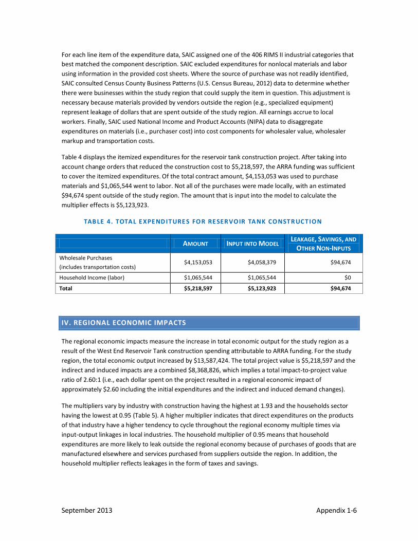
For each line item of the expenditure data, SAIC assigned one of the 406 RIMS II industrial categories that best matched the component description. SAIC excluded expenditures for nonlocal materials and labor using information in the provided cost sheets. Where the source of purchase was not readily identified, SAIC consulted Census County Business Patterns (U.S. Census Bureau, 2012) data to determine whether there were businesses within the study region that could supply the item in question. This adjustment is necessary because materials provided by vendors outside the region (e.g., specialized equipment) represent leakage of dollars that are spent outside of the study region. All earnings accrue to local workers. Finally, SAIC used National Income and Product Accounts (NIPA) data to disaggregate expenditures on materials (i.e., purchaser cost) into cost components for wholesaler value, wholesaler markup and transportation costs.
Table 4 displays the itemized expenditures for the reservoir tank construction project. After taking into account change orders that reduced the construction cost to $5,218,597, the ARRA funding was sufficient to cover the itemized expenditures. Of the total contract amount, $4,153,053 was used to purchase materials and $1,065,544 went to labor. Not all of the purchases were made locally, with an estimated $94,674 spent outside of the study region. The amount that is input into the model to calculate the multiplier effects is $5,123,923.
TAB LE 4. TOTAL E XPE ND ITURE S FOR RE SER VOIR TANK CONSTR UC TION
AMOUNT INPUT INTO MODEL LEAKAGE, SAVINGS, AND OTHER NON-INPUTS
Wholesale Purchases (includes transportation costs)
$4,153,053 $4,058,379 $94,674
Household Income (labor) $1,065,544 $1,065,544 $0
Total $5,218,597 $5,123,923 $94,674
IV. REGIONAL ECONOMIC IMPACTS
The regional economic impacts measure the increase in total economic output for the study region as a result of the West End Reservoir Tank construction spending attributable to ARRA funding. For the study region, the total economic output increased by $13,587,424. The total project value is $5,218,597 and the indirect and induced impacts are a combined $8,368,826, which implies a total impact-to-project value ratio of 2.60:1 (i.e., each dollar spent on the project resulted in a regional economic impact of approximately $2.60 including the initial expenditures and the indirect and induced demand changes).
The multipliers vary by industry with construction having the highest at 1.93 and the households sector having the lowest at 0.95 (Table 5). A higher multiplier indicates that direct expenditures on the products of that industry have a higher tendency to cycle throughout the regional economy multiple times via input-output linkages in local industries. The household multiplier of 0.95 means that household expenditures are more likely to leak outside the regional economy because of purchases of goods that are manufactured elsewhere and services purchased from suppliers outside the region. In addition, the household multiplier reflects leakages in the form of taxes and savings.
September 2013 Appendix 1-6

TAB LE 5. TOTAL OUTPUT BY IND USTRY B ASED ON R IMSII ANALY SIS
Forestry, Fishing
INDUSTRIAL
and
SECTOR
Hunting
REGIONAL PURCHASES
$13,052
MULTIPLIER
1.60
OUTPUT IMPACTS
$20,860
Mining $21,465 1.69 $36,373
Construction $1,743,120 1.93 $3,360,909
Manufacturing $1,812,089 1.74 $3,151,775
Wholesale Trade $218,522 1.58 $344,587
Transportation and Warehousing $158,706 1.82 $289,311
Professional and Technical Services $75,276 1.66 $125,279
Administrative and Waste Services $16,149 1.69 $27,359
Households $1,065,544 0.95 $1,012,373
Indirect and Induced Impacts $8,368,826
Total Project Value (including direct impact) $5,218,597
Total Output Impact $13,587,424
V. OTHER ENVIRONMENTAL AND ECONOMIC BENEFITS
The Hagerstown PWS provides drinking water for approximately 90,000 customers. It serves over 28,000 residences and businesses throughout the city and county (City of Hagerstown, no date). The PWS operates two conventional filtration plants (the R.C. Willson Water Treatment Plant and the W.M. Breichner Water Treatment Plant) to treat surface water from two sources (the Potomac River and the Edgemont Reservoir) (City of Hagerstown, 2012). The PWS has a peak production capacity of 15 million gallons per day (MGD), but produces an average of 11 MGD. It uses eight water storage tanks and four pump stations to distribute water throughout its 400 miles of water mains (City of Hagerstown, no date).
The ARRA-funded project partially replaced the 11 MG West End Reservoir with the 6.8 MG Hellane Park Water Tank (Spiker, 2012). This project was needed to meet drinking water regulations pertaining to covered storage of treated water. EPA required that all water storage facilities newly constructed after February 16, 1999 by large systems such as the Hagerstown PWS be covered under the Interim Enhanced Surface Water Treatment Rule (EPA, 1998). EPA then extended similar requirements to pre-existing storage facilities in the Long-Term 2 Interim Enhanced Surface Water Treatment Rule (EPA, 2006), which included storage facilities such as the West End Reservoir. Systems with existing uncovered storage needed to either provide covered storage or treat the water leaving the uncovered storage facility to levels that meet the standards for Cryptosporidium parvum by April 1, 2009.
Because the West End Reservoir was not covered, treated water stored in it was at risk of re-contamination from a variety of sources. Environmental risks included direct contact with water fowl, wet deposition of air contaminants during precipitation events, and direct storm water runoff into the reservoir. Man-made risks included illegal waste dumping, illegal swimming and intentional sabotage. Because the enclosed Hellane Park Water Tank protects treated water against these risks, it prevents exposure to contaminants that could cause a wide range of adverse health effects among customers.
September 2013 Appendix 1-7
In addition to ensuring drinking water quality, the Hagerstown PWS may also benefit from reduced operating costs. First, it avoids the added expense of having to re-treat all of the stored water to drinking water standards prior to distribution. In addition, it may be able to reduce chemical addition to the reservoir. The West End Reservoir had deteriorated to the extent that leakages led to daily losses of a minimum of 0.3 MG treated water (Spiker, 2012). This is the equivalent of the amount of water used by 3,000 people assuming an average daily per capita consumption of 100 gallons. The Hellane Park Water Tank ends a portion of this water loss. The related water savings reduces overall water production costs including costs for treatment chemicals, energy and sludge residuals that are the result of conventional filtration processes.
Water utility customers also benefit because the project funding included ARRA funds with a principal forgiveness. The City of Hagerstown originally planned to issue bonds to finance a portion of the project. After replacing that source with the ARRA funds, the City was able to reduce the long-term debt associated with the overall Hagerstown PWS capital investment plan. This savings can either reduce utility rates or it can allow the utility to incur debt for other projects that will continue to improve and expand overall service. Michael Spiker, Director of Utilities for Hagerstown, says that by reducing the amount of long term-debt incurred for the project, the favorable financing conditions have aided in allowing the utility to establish a Repair, Renewal and Replacement (3R) Reserve Fund to address aging infrastructure.
September 2013 Appendix 1-8

REFERENCES
Bureau of Economic Analysis (BEA). 2012a. Data from U.S. Census Bureau accessed on BEA website on November 9, 2012. http://www.bea.gov/regional/
BEA. 2012b. "Decennial Census, 2000 and 2010”. "Local Area Personal Income & Employment" Interactive tables on website. Accessed November 9, 2012. http://www.bea.gov/regional/
BEA. 2012c. RIMS II: An essential tool for regional developers and planners. Washington, D.C.; U.S. Government Printing Office.
BEA. 2012d. RIMS II Multipliers 2002/2010: Table 1.5, Total Multipliers for Output by Detailed Industry, Custom Study Region (Type II). November 2012.
City of Hagerstown. 2012. Consumer Confidence Report. Available online at http://www.hagerstownmd.org/DocumentCenter/Home/View/1183, accessed November 2012.
City of Hagerstown. No date. Utilities Department slide presentation. Available online at http://www.hagerstownmd.org/DocumentCenter/Home/View/1205, accessed November 2012.
City of Hagerstown. Photo of tank construction. Available online at http://www.hagerstownmd.org/PhotoViewScreen.aspx?PID=42, accessed November 2012.
EPA. 1998. National Primary Drinking Water Regulations: Interim Enhanced Surface Water Treatment; Final Rule. Federal Register 63 (69478), December 16, 1998.
EPA. 2006. National Primary Drinking Water Regulations: Long Term 2 Enhanced Surface Water Treatment Rule; Final Rule. Federal Register 71 (654), January 5, 2006.
Spiker, M. 2012. Personal communication with SAIC. November 30, 2012.
U.S. Census Bureau. 2012. County Business Patterns, 2010 for Frederick, MD; Washington, MD; Adams, PA; Franklin, PA; Fulton, PA; Berkeley, WV; Jefferson, WV; and Morgan, WV counties. http://www.census.gov/econ/cbp/, accessed August 15, 2012.
September 2013 Appendix 1-9

This page intentionally blank.
September 2013 Appendix 1-10

APPENDIX 2: AMSTERDAM DRINKING WATER TREATMENT PLANT UPGRADES

This page intentionally blank.

I. PROJECT DESCRIPTION
The City of Amsterdam is located in Montgomery County, New York about 35 miles northwest of the City of Albany. The project area consists of the Albany-Schenectady-Troy metropolitan statistical area (MSA) plus Fulton County and Montgomery County.
In 2009, the City of Amsterdam received $10.6 million to support the planning, design and construction for a major upgrade of the city’s existing drinking water treatment plant in order to meet current standards. The funding comprised $10.5 million in total SRF support including almost $5.1 million in ARRA funding. Therefore, the nonfederal funding of $100,000 is highly leveraged.
The original drinking water plant, built in 1974, consisted of direct filtration. It could not meet the water quality standards for haloacetic acid (HAA5) levels and total trihalomethanes (TTHM) (City of Amsterdam, 2009). Furthermore, the plant provided wholesale water to a purchasing system, the Town of Amsterdam, which had a violation for TTHM in 2009 (Town of Amsterdam, 2010). Finally, in 2008, the plant was also unable to meet standards for lead in the City of Amsterdam (City of Amsterdam, 2009).
The upgrade included a new sedimentation/clarification process to improve pre-filter solids removal, a new ultraviolet (UV) disinfection system, a new carbon contact system for taste and odor control, corrosion control treatment, and a multi-level intake system at the city’s Steele Reservoir. In addition, the existing degrading filter backwash water supply tank was demolished and replaced with a new bolted steel tank. Other facility improvements include emergency standby generators, a new high-efficiency space conditioning system, existing roof repairs, and upgrades to the existing computer control system. The project also incorporated improvements to the city's raw water source including rehabilitation of a portion of the raw water transmission main. The upgrades are expected to double the existing system's capacity to 12 million gallons per day and improve drinking water quality for the city’s approximately 19,000 residents (John M. McDonald Engineering, 2012).
II. REGION DESCRIPTION
The study region (Figure 1) consists of seven jurisdictions in upper New York, five of which are within the Albany-Schenectady-Troy MSA. The City of Amsterdam is located in Montgomery County about 35 miles northwest of the City of Albany. The market area reaches the boundaries of Massachusetts and Vermont, but only includes counties within the State of New York to remain consistent with the economically independent defined MSA.
September 2013 Appendix 2-1

F IGURE 1. C ITY OF AMSTER DAM PWS EC ONOMIC IMPACT STUDY REGION
September 2013 Appendix 2-2

The study region includes Fulton County and Montgomery County plus all of the Albany-Schenectady-Troy MSA: Albany County, Rensselaer County, Saratoga County, Schenectady County and Schoharie County.
POPULATION
Table 1 reports population data for the study region components. In aggregate, the population in the communities within the study area increased 4.8 percent between 2000 and 2010. The growth has been strong in three of the counties with Saratoga, Schenectady and Rensselaer gaining above 4 percent. Population growth in Fulton and Montgomery was essentially flat and Schoharie and Albany increased at a modest 3.7 and 3.0 percent, respectively.
TAB LE 1. POPULATION CH ANGE S IN SELE CTED ARE AS, 2000- 2010
COUNTY POPULATION PERCENT CHANGE, 2000-2010
2000 2010 TOTAL ANNUAL
Albany, NY 295,106 303,889 3.0% 0.3% Fulton, NY 54,976 55,471 0.9% 0.1% Montgomery, NY 49,605 50,260 1.3% 0.1% Rensselaer, NY 152,684 159,465 4.4% 0.4% Saratoga, NY 201,514 219,988 9.2% 0.9% Schenectady, NY 146,581 154,932 5.7% 0.6% Schoharie, NY 31,514 32,692 3.7% 0.4% Total 931,980 976,697 4.8% 0.5% Source: BEA, 2012a
LOCAL ECONOMY
Within the study region, local and state government is a significant portion of the full- and part-time employment accounting for 17.7 percent of total employment (Table 2). Next, healthcare and social assistance each account for 13 percent of employment, and retail trade accounts for 10.7 percent. The presence of Albany, the state capital of New York, results in a higher concentration of state and federal government employees within the Albany MSA.
Montgomery County is more reliant on manufacturing than other jurisdictions in the region. The manufacturing sector accounts for more than 14 percent of countywide employment, but this sector makes up less than 5 percent of total employment throughout the region. Furthermore, Montgomery County accounts for more than 12 percent of regional employment in the manufacturing sector, despite having less than 3 percent of regional jobs.
September 2013 Appendix 2-3

TAB LE 2. E MPLOY ME NT BY IND USTR IAL SE CTOR , 2010
INDUSTRIAL SECTOR FULTON MONTGOMERY ALBANY MSA AREAS1 TOTAL
Total Employment 27,093 22,485 535,201 584,779
Farm Employment 256 774 2,832 3,862
Forestry, Fishing and Hunting (D) 79 (D) 79
Mining (D) 101 (D) 101
Utilities (D) (D) (D) -
Construction 1,815 937 25,036 27,788
Manufacturing 1,938 3,327 21,544 26,809
Wholesale Trade (D) (D) 13,514 13,514
Retail Trade 3,472 3,102 56,071 62,645
Transportation and Warehousing 1,586 1,445 (D) 3,031
Information 469 329 10,261 11,059
Finance and Insurance 883 541 32,183 33,607
Real Estate, Rental and Leasing 1,316 410 20,884 22,610
Professional and Technical Services 971 437 41,455 42,863
Management of Companies 182 303 6,877 7,362
Administrative and Waste Services 816 291 20,647 21,754
Educational Services 217 89 22,537 22,843
Health Care and Social Assistance 4,118 4,321 67,842 76,281
Arts, Entertainment and Recreation 451 201 10,795 11,447
Accommodation and Food Services 1,323 1,352 31,509 34,184
Other Services 1,774 941 25,259 27,974
Federal Government, Civilian 121 118 7,240 7,479
Military 89 80 3,117 3,286
State and Local Government 4,347 2,743 96,340 103,430
Source: BEA, 2012b Note: Totals include employment that is not displayed in the sector breakout because of non-disclosure issues. 1. Includes the following counties: Albany, Rensselaer, Saratoga, Schenectady and Schoharie.
September 2013 Appendix 2-4
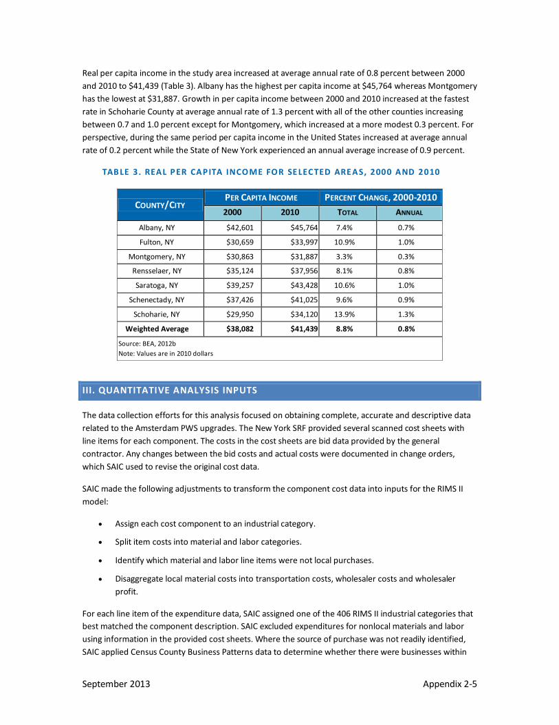
Real per capita income in the study area increased at average annual rate of 0.8 percent between 2000 and 2010 to $41,439 (Table 3). Albany has the highest per capita income at $45,764 whereas Montgomery has the lowest at $31,887. Growth in per capita income between 2000 and 2010 increased at the fastest rate in Schoharie County at average annual rate of 1.3 percent with all of the other counties increasing between 0.7 and 1.0 percent except for Montgomery, which increased at a more modest 0.3 percent. For perspective, during the same period per capita income in the United States increased at average annual rate of 0.2 percent while the State of New York experienced an annual average increase of 0.9 percent.
TAB LE 3. REAL PER CAPITA INCOME FOR SE LEC TED ARE AS, 2000 AND 2010
COUNTY/CITY PER CAPITA INCOME PERCENT CHANGE, 2000-2010 2000 2010 TOTAL ANNUAL
Albany, NY $42,601 $45,764 7.4% 0.7%
Fulton, NY $30,659 $33,997 10.9% 1.0%
Montgomery, NY $30,863 $31,887 3.3% 0.3%
Rensselaer, NY $35,124 $37,956 8.1% 0.8%
Saratoga, NY $39,257 $43,428 10.6% 1.0%
Schenectady, NY $37,426 $41,025 9.6% 0.9%
Schoharie, NY $29,950 $34,120 13.9% 1.3%
Weighted Average $38,082 $41,439 8.8% 0.8%
Source: BEA, 2012b Note: Values are in 2010 dollars
III. QUANTITATIVE ANALYSIS INPUTS
The data collection efforts for this analysis focused on obtaining complete, accurate and descriptive data related to the Amsterdam PWS upgrades. The New York SRF provided several scanned cost sheets with line items for each component. The costs in the cost sheets are bid data provided by the general contractor. Any changes between the bid costs and actual costs were documented in change orders, which SAIC used to revise the original cost data.
SAIC made the following adjustments to transform the component cost data into inputs for the RIMS II model:
• Assign each cost component to an industrial category.
• Split item costs into material and labor categories.
• Identify which material and labor line items were not local purchases.
• Disaggregate local material costs into transportation costs, wholesaler costs and wholesaler profit.
For each line item of the expenditure data, SAIC assigned one of the 406 RIMS II industrial categories that best matched the component description. SAIC excluded expenditures for nonlocal materials and labor using information in the provided cost sheets. Where the source of purchase was not readily identified, SAIC applied Census County Business Patterns data to determine whether there were businesses within
September 2013 Appendix 2-5

the study region that could supply the item in question. This adjustment is necessary because materials provided by vendors outside the region (e.g., filtration package plant) represent leakage of dollars that are spent outside of the study region. Finally, SAIC used National Income and Product Accounts (NIPA) data to disaggregate expenditures on materials (i.e., purchaser cost) into cost components for wholesaler value, wholesaler markup and transportation costs.
Table 4 displays the total expenditures for the PWS Upgrade project. The total contract amounts to $10,647,863 including change orders. ARRA funding accounted for nearly half of the value of the project with $5,081,049 provided in the form of a principal-forgiven loan. Of the total contract amount, $7,077,431 was used to purchase materials, $3,020,432 went to labor costs, and $550,000 was applied to insurance, bonding, and mobilization. Not all of the purchases were made locally, with an estimated $3,908,613 spent outside of the study region. The amount that is input into the model to calculate the multiplier effects is $6,739,250.
TAB LE 4. TOTAL E XPE ND ITURE S FOR PWS UPGR AD E
AMOUNT INPUT INTO MODEL
LEAKAGE, SAVINGS AND OTHER NON-INPUTS
Wholesale Purchases (includes transportation costs)
$7,077,431 $3,718,817 $3,358,613
Household Income (labor) $3,020,432 $3,020,432 $604,086
Other $550,000 $0 $550,000
Total $10,647,863 $6,739,250 $4,512,700
Note: Values are in 2008 dollars
IV. REGIONAL ECONOMIC IMPACTS
The regional economic impacts measure the increase in total economic output for the study region as a result of the Amsterdam PWS upgrades. For the study region, the total economic output increased by $19,889,366. The total project value is $10,647,863 and the indirect and induced impacts are a combined $9,241,503, which implies a total impact-to-project value ratio of 1.87:1 (i.e., each dollar spent on the project resulted in a regional economic impact of approximately $1.87 including the initial expenditures and the indirect and induced demand changes). The region applied in this analysis represents the area where the expenditures and labor were procured. However, many of the materials used in the project were manufactured outside of the region. The smaller study region most likely results in a lower total impact-to-project value ratio because spending leakages are likely given the size of the local economy.
The multipliers vary by industry with construction and finance and insurance sectors having the highest at 1.87 and the households sector having the lowest at 0.96 (Table 5). A higher multiplier indicates that direct expenditures on the products of that industry have a higher tendency to cycle throughout the regional economy multiple times via input-output linkages in local industries. The household multiplier of 0.96 indicates that household expenditures are more likely to leak outside the regional economy because of purchases of goods that are manufactured elsewhere and services purchased from suppliers outside the region. In addition, the households multiplier reflects leakages in the form of taxes and savings.
September 2013 Appendix 2-6
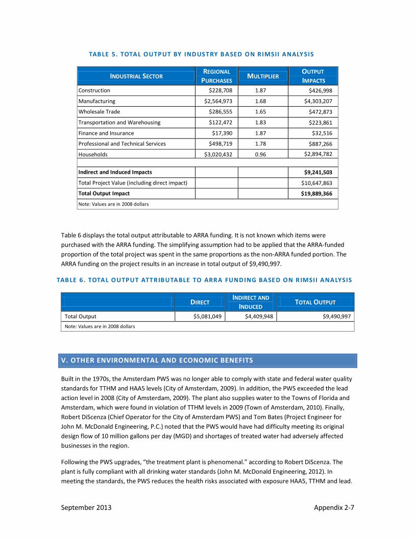
TAB LE 5. TOTAL OUTPUT BY IND USTRY B ASED ON R IMSII ANALY SIS
INDUSTRIAL SECTOR REGIONAL PURCHASES MULTIPLIER OUTPUT
IMPACTS Construction $228,708 1.87 $426,998
Manufacturing $2,564,973 1.68 $4,303,207
Wholesale Trade $286,555 1.65 $472,873
Transportation and Warehousing $122,472 1.83 $223,861
Finance and Insurance $17,390 1.87 $32,516
Professional and Technical Services $498,719 1.78 $887,266
Households $3,020,432 0.96 $2,894,782 Indirect and Induced Impacts $9,241,503
Total Project Value (including direct impact) $10,647,863
Total Output Impact $19,889,366
Note: Values are in 2008 dollars
Table 6 displays the total output attributable to ARRA funding. It is not known which items were purchased with the ARRA funding. The simplifying assumption had to be applied that the ARRA-funded proportion of the total project was spent in the same proportions as the non-ARRA funded portion. The ARRA funding on the project results in an increase in total output of $9,490,997.
TAB LE 6. TOTAL OUTPUT ATTR IB UTABLE TO ARR A FUND ING BASE D ON R IMSII ANALYSIS
DIRECT INDIRECT AND INDUCED TOTAL OUTPUT
Total Output $5,081,049 $4,409,948 $9,490,997
Note: Values are in 2008 dollars
V. OTHER ENVIRONMENTAL AND ECONOMIC BENEFITS
Built in the 1970s, the Amsterdam PWS was no longer able to comply with state and federal water quality standards for TTHM and HAA5 levels (City of Amsterdam, 2009). In addition, the PWS exceeded the lead action level in 2008 (City of Amsterdam, 2009). The plant also supplies water to the Towns of Florida and Amsterdam, which were found in violation of TTHM levels in 2009 (Town of Amsterdam, 2010). Finally, Robert DiScenza (Chief Operator for the City of Amsterdam PWS) and Tom Bates (Project Engineer for John M. McDonald Engineering, P.C.) noted that the PWS would have had difficulty meeting its original design flow of 10 million gallons per day (MGD) and shortages of treated water had adversely affected businesses in the region.
Following the PWS upgrades, “the treatment plant is phenomenal.” according to Robert DiScenza. The plant is fully compliant with all drinking water standards (John M. McDonald Engineering, 2012). In meeting the standards, the PWS reduces the health risks associated with exposure HAA5, TTHM and lead.
September 2013 Appendix 2-7

Exposure to disinfection byproducts such as HAA5 and TTHM can increase the risk of bladder, colon and rectal cancers, and also increase the risk of reproductive and developmental effects (EPA, 2006). In addition, the new corrosion control system should reduce lead levels in households that have lead service lines and plumbing. Reduced exposure to lead in drinking water reduces risks of damage to the brain and kidneys, and interference with the production of red blood cells that carry oxygen, especially among infants, children and pregnant women (EPA, 2007). The PWS also benefits from no longer having to notify its customers of health standard violations.
Maintaining compliance with drinking water quality standards improves customer relations, and DiScenza and Bates commented that it also benefits efforts to attract businesses to the region. In addition to providing short-term benefits for the local economy, the PWS upgrades contribute to medium- and long-term economic benefits and support future economic development. Local businesses will also benefit from improved water quality. For example, in June 2010, Beech-Nut opened a new $124 million plant in Montgomery County (Beech-Nut, 2012). This manufacturer initially requested up to 1.5 MGD of the treated water for its baby food production plant, which would have been a difficult demand to meet prior to the upgrades. Having a reliable source of high quality water reduces Beech-Nut’s cost for on-site water treatment. The plant may also result in indirect economic benefits in the local community if it fulfills its plan to use locally sourced food products.
The capacity constraints of the original plant also adversely affected growth potential. With higher production capacity, the municipalities served by the Amsterdam PWS can consider extending their service areas, which encourages economic growth.
The upgrades also have some environmental benefits related to water efficiency and renewable energy use. The PWS has lower filter backwash discharges because fewer solids reach the filters; the upflow clarifiers remove solids prior to filtering. The PWS was also able to upgrade a hydro-powered turbine that generates enough power to operate pumps, saving the utility up to $80,000 in avoided annual power expenses (DiScenza and Bates, 2012).
REFERENCES
Beech-Nut. www.beechnut.com/About%20Us/itn_newProductionFacility.asp. Accessed August 22, 2012.
Bureau of Economic Analysis (BEA). 2012a. Data from U.S. Census Bureau accessed on BEA website on August 3, 2012. http://www.bea.gov/regional/
BEA. 2012b. "Decennial Census, 2000 and 2010”. "Local Area Personal Income & Employment" Interactive tables on website. Accessed August 3, 2012. http://www.bea.gov/regional/
BEA. 2012c. RIMS II: An essential tool for regional developers and planners. Washington, D.C.; U.S. Government Printing Office.
BEA. 2012d. RIMS II Multipliers 2002/2008: Table 1.5, Total Multipliers for Output by Detailed Industry, Custom Study Region (Type II). July 2012.
The Buzz: Business news - timesunion.com. blog.timesunion.com/business/ticker-beech-nuts-new-plant-now-operating/20004. Accessed August 22, 2012.
September 2013 Appendix 2-8

City of Amsterdam. 2009. 2009 Annual Report for 2008 Drinking Water Quality.
DiScenza, Robert and Tom Bates. Personal communication with SAIC, September 25, 2012.
EPA. 2006. “National Primary Drinking Water Regulations: Stage 2 Disinfectants and Disinfection Byproducts Rule.” 71 Federal Register 388 (January 4, 2006).
EPA. 2007. “National Primary Drinking Water Regulations for Lead and Copper: Short-Term Regulatory Revisions and Clarifications.” 72 Federal Register 57782 (October 10, 2007).
John M. McDonald Engineering, P.C. Project Descriptions. www.mcdonaldengineers.com/past-projects/water. Accessed June 13, 2012.
Perez, D. 2010. “Amsterdam prepares for Beech-Nut’s arrival.” Your News Now, June 9, 2010. http://capitalregion.ynn.com/content/headlines/507487/amsterdam-prepares-for-beech-nut-s-arrival/. Accessed September 6, 2012.
Town of Amsterdam. 2010. Annual Drinking Water Quality Report for 2009.
September 2013 Appendix 2-9

This page intentionally blank.
September 2013 Appendix 2-10

APPENDIX 3: ATHENS DRINKING WATER DISTRIBUTION SYSTEM IMPROVEMENT

This page intentionally blank.

I. PROJECT DESCRIPTION
Athens County is located in eastern Ohio with the county seat in the City of Athens, which is located about 72 miles southeast of the City of Columbus, Ohio. The City received $320,000 in ARRA funding to repair and replace part of the drinking water utility’s distribution system. The ARRA funding included $320,000 of principal forgiveness. Additional funding for the project included $480,000 in other State Revolving Fund financing and up to $75,000 in other resources to cover the initial project cost of $875,000.
In 2010, the ARRA-funded Curtis Street and Mulligan Road project replaced 3,700 feet of 8- and 12-inch service lines that deliver water to a storage tower as well as distribute water in a residential area. The project also replaced a pump station. The service line for the tower in the Curtis Street and Mulligan Road area was old and prone to breakage. In addition, the electrical system that supports that part of the distribution network is older and prone to electrical fluctuations. These fluctuations could alter pumping pressures and cause water hammer – a surge in water pressure that can damage pipes. Thus, the project addressed both sources of frequent line breaks, which were almost a monthly occurrence (Stone, 2012).
II. REGION DESCRIPTION
Based on a recommendation of staff at the Athens Department of Public Works, the study region (Figure 2) contains two counties in Ohio: Athens and Washington (Adine, 2012). This recommendation was based on the belief that all labor and materials came from these counties. These two rural counties share a contiguous boundary with West Virginia and are located within 1.5 hours of Columbus, OH. Because both counties are rural and located near a major urban area, it is possible that some household expenditures occur outside the region and, therefore, will not be captured in the analysis.
September 2013 Appendix 3-1

F IGURE 1. ATH E NS DR INKING WATE R D ISTR IB UTION SYSTE M EC ONOMIC IMPACT STUDY REGION
September 2013 Appendix 3-2

POPULATION
Table 1 reports population data for the study region components. In aggregate, the population in the communities within the study area grew by 0.1 percent annually between 2000 and 2010. All of the growth occurred in Athens County where population increased at an average annual rate of 0.4 percent. Population declined, however, in Washington County at an average annual rate of 0.2 percent.
TAB LE 1. POPULATION CH ANGE S IN SELE CTED ARE AS, 2000- 2010
COUNTY POPULATION PERCENT CHANGE, 2000-2010
2000 2010 TOTAL ANNUAL
Athens, OH 62,324 64,774 3.9% 0.4%
Washington, OH 63,180 61,716 -2.3% -0.2%
Total 125,504 126,490 0.8% 0.1%
Source: BEA, 2012a
LOCAL ECONOMY
Within the study, region, state and local government accounts for over one-third of the full- and part-time workers in 2010 (Table 2). This share remained almost constant over the period. Other key employment industries in 2010 include retail trade (12.1 percent) and health care and social assistance (11.2 percent). Together, these three industries account for almost 60 percent of total employment.
Overall, there was a net gain of 2,025 jobs or approximately 7.3 percent of 2001 employment. Employment trends varied substantially across sectors. Employment growth rates ranged from net losses above 22 percent in the farming industry and the forestry, fishing and hunting industry to net gains of almost 50 percent in the real estate, rental and leasing industry. There is insufficient data to make a valid comparison among sectors such as the construction and manufacturing sectors that do not have data available for one of the years. The state and local government sector added the most employees between 2001 and 2010 with over 835 new employees (an increase of 8.6 percent).
September 2013 Appendix 3-3

TAB LE 2. E MPLOY ME NT BY IND USTR IAL SE CTOR , 2001 AND 2010
INDUSTRIAL SECTOR 2001 2010 PERCENT OF TOTAL 2001 2010
Total Employment 27,834 29,859 100.0% 100.0%
Farm Employment 709 548 2.5% 1.8%
Forestry, Fishing and Hunting 119 92 0.4% 0.3%
Mining 83 (D) 0.3% (D)
Utilities 90 83 0.3% 0.3%
Construction 1,144 (D) 4.1% (D)
Manufacturing 1,111 (D) 4.0% (D)
Wholesale Trade 293 400 1.1% 1.3%
Retail Trade 3,279 3,609 11.8% 12.1%
Transportation and Warehousing 331 305 1.2% 1.0%
Information 387 401 1.4% 1.3%
Finance and Insurance 640 674 2.3% 2.3%
Real Estate, Rental and Leasing 568 847 2.0% 2.8%
Professional and Technical Services 935 1,061 3.4% 3.6%
Management of Companies (D) 86 (D) 0.3%
Administrative and Waste Services (D) 613 (D) 2.1%
Educational Services 291 335 1.0% 1.1%
Health Care and Social Assistance 2,975 3,339 10.7% 11.2%
Arts, Entertainment and Recreation 495 440 1.8% 1.5%
Accommodation and Food Services 2,262 2,502 8.1% 8.4%
Other Services 1,338 1,372 4.8% 4.6%
Federal Government, Civilian 253 265 0.9% 0.9%
Military 181 174 0.7% 0.6%
State and Local Government 9,755 10,590 35.0% 35.5%
Source: BEA, 2012b (D) = not displayed because of non-disclosure issues. Note: Totals include employment that is not displayed in the sector breakout because of non-disclosure issues.
September 2013 Appendix 3-4

Real per capita income in the study area increased at average annual rate of 1.0 percent between 2000 and 2010 (Table 3). For perspective, during the same period per capita income in the United States increased at average annual rate of 0.2 percent while the State of Ohio experienced an annual average decrease of 0.3 percent. In 2010, Washington County has a substantially higher real per capita income of $32,134 compared to Athens County’s real per capita income of $26,296.
TAB LE 3. REAL PER CAPITA INCOME FOR SE LEC TED ARE AS, 2000 AND 2010
COUNTY/CITY PER CAPITA INCOME PERCENT CHANGE, 2000-2010
1990 2002 2000 2010 TOTAL ANNUAL
Athens, OH $23,477 $26,296 12.0% 1.1%
Washington, OH $29,395 $32,134 9.3% 0.9%
Weighted Average $26,456 $29,144 10.2% 1.0%
Source: BEA, 2012b Note: Values are in 2010 dollars.
III. QUANTITATIVE ANALYSIS INPUTS
The data collection efforts for this analysis focused on obtaining complete, accurate and descriptive data related to the Curtis Street and Mulligan Road construction project. The City of Athens Department of Public Works provided a detailed invoice with line items for each component. The costs in the document are bid data provided by the general contractor.
SAIC made the following adjustments to transform the component cost data into inputs for the RIMS II model (BEA, 2012c):
• Assign each cost component to an industrial category.
• Split item costs into material and labor categories.
• Identify which material and labor line items were not local purchases, if any.
• Disaggregate local material costs into transportation costs, wholesaler costs and wholesaler profit.
For each line item of the expenditure data, SAIC assigned one of the 406 RIMS II industrial categories that best matched the component description. Where the source of purchase was not readily identified, SAIC applied Census County Business Patterns (U.S. Census Bureau, 2012) data to determine whether there were businesses within the study region that could supply the item in question. This adjustment is necessary because materials provided by vendors outside the region (e.g., specialized equipment) represent leakage of dollars that are spent outside of the study region. Finally, SAIC used National Income and Product Accounts (NIPA) data to disaggregate expenditures on materials (i.e., purchaser cost) into cost components for wholesaler value, wholesaler markup and transportation costs.
Table 4 displays the itemized expenditures for the water line and pump station construction. For the total contract amount of $821,832, $528,129 was used to purchase materials and $293,703 went to labor. Because all expenditures for this project are local, the entire project value of $821,832 is considered as a
September 2013 Appendix 3-5

direct impact and is input into the model to calculate the multiplier effects.
TAB LE 4. TOTAL E XPE ND ITURE S FOR WATER L INE AND PUMP STATION
AMOUNT Wholesale Purchases (includes transportation costs) $528,129
Household Income (labor) $293,703
Total $821,832
Note: Values are in 2010 dollars.
IV. REGIONAL ECONOMIC IMPACTS
The regional economic impacts measure the increase in total economic output for the study region as a result of the Curtis Street and Mulligan Road construction spending attributable to ARRA funding. For the study region, the total economic output increased by $1,375,984. The total project value is $821,832 and the indirect and induced impacts are a combined $554,153, which implies a total impact-to-project value ratio of 1.67:1 (i.e., each dollar spent on the project resulted in a regional economic impact of approximately $1.67 including the initial expenditures and the indirect and induced demand changes). The region applied in this analysis represents the area where the expenditures and labor were procured. However, many of the materials used in the project were manufactured outside of the region. The smaller study region most likely results in a lower total impact-to-project value ratio because spending leakages are likely given the size of the local economy.
The multipliers vary by industry with the construction sector having the highest at 1.59 and the manufacturing sector having the lowest at 0.14 (Table 5). A higher multiplier indicates that direct expenditures on the products of that industry have a higher tendency to cycle throughout the regional economy multiple times via input-output linkages in local industries. The manufacturing multiplier of 0.14 indicates that most of the materials used in this project use inputs that were manufactured outside of the study region. This lack of second-order industry linkages results in almost no recirculation of initial manufacturing expenditures within the study region. Additionally, the household multiplier of 0.73 means that household expenditures are more likely to leak outside the regional economy because of purchases of goods that are manufactured elsewhere and services purchased from suppliers outside the region. In addition, the household multiplier reflects leakages in the form of taxes and savings.
September 2013 Appendix 3-6

TAB LE 5. TOTAL OUTPUT BY IND USTRY B ASED ON R IMSII ANALY SIS
INDUSTRIAL SECTOR REGIONAL PURCHASES MULTIPLIER OUTPUT
IMPACTS Construction $72,415 1.59 $114,994
Manufacturing $360,840 0.14 $52,010
Wholesale Trade $108,974 1.35 $147,246
Transportation and Warehousing $26,576 1.46 $38,861
Professional and Technical Services $7,663 1.44 $11,052
Administrative and Waste Services $17,000 1.36 $23,147
Households $228,364 0.73 $166,843
Indirect and Induced Impacts $554,153
Total Project Value (including direct impact) $821,832
Total Output Impact $1,375,984
Note: Values are in 2010 dollars. Totals may not add to detail because of independent rounding.
Table 6 displays the total output attributable to ARRA funding. It is not known which items were purchased with the ARRA funding. The simplifying assumption had to be applied that the industry allocation of the ARRA funds is the same as the overall project allocation shown in Table 5. Therefore, the ratio of total impacts-to-ARRA funding is also the same. The ARRA funding on the project results in an increase in total output of $535,772.
TAB LE 6. TOTAL OUTPUT ATTR IB UTABLE TO ARR A FUND ING BASE D ON R IMSII ANALYSIS
DIRECT INDIRECT AND INDUCED TOTAL OUTPUT
Total Output $320,000 $215,772 $535,772 Note: Values are in 2010 dollars
V. OTHER ENVIRONMENTAL AND ECONOMIC BENEFITS
The Athens Water Department has provided drinking water to residents since 1894 (AOWD, 2012). According to Andrew Stone, Director of Public Works, the system has grown over time throughout a hilly area, and as a result has a variety of pressure zones as well as aging infrastructure that deliver 3 million gallons per day (MGD) to its customers. One of the older parts of the distribution system, in particular, was a source of frequent pipeline breaks.
The highest point of the city has a small water storage tower, Longview Tower, which serves southwest Athens. At 0.2 million gallons (MG), the tower capacity is small relative to demand and, therefore ’turns over‘ several times a day. The service line for the tower in the Curtis Street and Mulligan Road area was old and prone to breakage. In addition, the electrical system that supports that part of the distribution network is older and prone to electrical fluctuations. These fluctuations affect pumping pressures, which can cause water hammer – a surge in water pressure that can damage pipes. Thus, there are multiple causes of frequent pipe breaks.
September 2013 Appendix 3-7

These breaks are problematic. They can result in temporary service interruptions for up to 500 households. Depending on the extent of the pressure loss, the repair can be followed by mandatory boil alerts. Finally, depending on the break location and severity, up to 0.3 MG of water can flood low-lying residential areas when the water from the tower and supply lines empties through the break (Stone, 2012).
The ARRA-funded Curtis Street and Mulligan Road project replaced 3,700 feet of 8- and 12-inch service lines for the tower and replaced the pump station. Thus, the project addressed both sources of frequent line breaks, which were almost a monthly occurrence. The ARRA funding was important to successfully implement this particular line upgrade because the cost exceeded the system’s typical annual budget of $0.4 million for line replacement (Stone, 2012). The system had nominated the project for the State Revolving Fund for several years and finally received support including ARRA funding.
There are several different kinds of economic benefits because the project has ended pipe breaks in this portion of the water distribution system. First and foremost, ending pipe breaks avoids any potential for health risk of drinking water contaminated via the break. It also reduces the nuisance of complying with boil alerts; secondary benefits of not having to issue boil alerts consist of improved customer relations and reduced administrative costs of handling the alerts and any subsequent complaints about the break, service loss, flooding and boil alerts. Additional benefits include avoided property damages to the residences at risk of flooding caused by pipeline breaks. Finally, the system no longer incurs the repair costs and saves on production costs because it avoids the large water losses that could accompany a pipe break in this area. For example, if a break results in a loss of 0.3 MG of water, then the loss is equivalent to 10% of one day’s production. Given an annual electricity cost of $375,000 for plant operation and distribution pumping, a break represents approximately $100 in wasted electricity expenditures (Stone, 2012).
The Curtis Street and Mulligan Road area of the distribution system serves a residential area. Therefore, there are no known benefits in terms of current economic benefits for commercial or industrial customers aside from the production cost savings associated with reductions in annual water loss. All customers, however, potentially benefit from lower water rates for two reasons. First, the principal forgiveness subsidy of the ARRA funding reduces the utility’s debt and payback requirements, which lowers rates. Also, lower production costs contribute to lower rates.
There are indirect environmental benefits associated with the savings in production costs that are associated with avoiding large water losses. An energy loss on the order of $100 per break noted above translates into 1400 kWh (kilowatt hour) of wasted treatment plant and pumping energy at an average power cost of $0.07 per kWh. There are most likely environmental externalities associated with power production (e.g., air emissions from coal or natural gas generation).
There are no other readily identifiable environmental benefits associated with the project (Stone, 2012). The water loss associated with breaks is not known to enter surface waters soon enough for the chlorine residual to have an ecosystem effect. The leaking water most likely infiltrates in pervious areas or is sufficiently diluted in the separate storm water system before it reaches discharge points. If it did discharge to surface waters, the chlorinated water could have adverse effect on aquatic ecosystems. For example, a recent fish kill occurred after chlorinated water flushed from a line elsewhere in the system entered a stream.
September 2013 Appendix 3-8
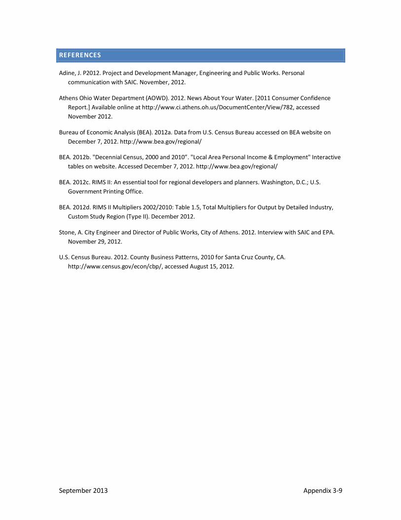
REFERENCES
Adine, J. P2012. Project and Development Manager, Engineering and Public Works. Personal communication with SAIC. November, 2012.
Athens Ohio Water Department (AOWD). 2012. News About Your Water. [2011 Consumer Confidence Report.] Available online at http://www.ci.athens.oh.us/DocumentCenter/View/782, accessed November 2012.
Bureau of Economic Analysis (BEA). 2012a. Data from U.S. Census Bureau accessed on BEA website on December 7, 2012. http://www.bea.gov/regional/
BEA. 2012b. "Decennial Census, 2000 and 2010”. "Local Area Personal Income & Employment" Interactive tables on website. Accessed December 7, 2012. http://www.bea.gov/regional/
BEA. 2012c. RIMS II: An essential tool for regional developers and planners. Washington, D.C.; U.S. Government Printing Office.
BEA. 2012d. RIMS II Multipliers 2002/2010: Table 1.5, Total Multipliers for Output by Detailed Industry, Custom Study Region (Type II). December 2012.
Stone, A. City Engineer and Director of Public Works, City of Athens. 2012. Interview with SAIC and EPA. November 29, 2012.
U.S. Census Bureau. 2012. County Business Patterns, 2010 for Santa Cruz County, CA. http://www.census.gov/econ/cbp/, accessed August 15, 2012.
September 2013 Appendix 3-9

This page intentionally blank.
September 2013 Appendix 3-10

APPENDIX 4: PINE BLUFFS METER INSTALLATION

This page intentionally blank.

I. PROJECT DESCRIPTION
The Town of Pine Bluffs is located in Laramie County, Wyoming. It is about 42 miles east of the City of Cheyenne and lies adjacent to the Wyoming-Nebraska border. The project area consists of Laramie County, which corresponds with the Cheyenne, WY metropolitan statistical area (MSA).
In 2009, the Town of Pine Bluffs received approximately $1.0 million in ARRA funding, most of which was used for a meter replacement project. The town needed to replace substantially malfunctioning water meters that were no longer working properly or were not used. The ARRA funding included $755,304 of principal forgiveness and a 20-year loan of $251,768 with 0% interest.
The project consisted of replacing substantially malfunctioning or nonfunctioning water meters. Poor meter reliability prevented the town from implementing conservation measures because it could not bill customers based on water consumption. Instead, the town had to charge a flat rate for water, which resulted in overconsumption. Facing water supply shortages, the town’s goal for the project was to improve conservation via a new use-based water billing system and leak detection monitoring. The project qualified for Green Project Reserve funding because of the expected energy savings and water savings associated with future reductions in unaccounted water losses and water conservation among customers.
II. REGION DESCRIPTION
The study region (Figure 1) consists of Laramie County which is in the southeast corner of Wyoming. The study area was limited to one county because the labor for the project and the locally supplied materials are all confined to Laramie County. A large portion of the expenditures, however, paid for metering materials that are manufactured outside of Wyoming. In addition, the wholesaler of the metering equipment (the only major wholesaler of such equipment in the state) is located in Casper, which is more than 200 miles northwest of the Town of Pine Bluffs in Natrona County, which is not part of the Cheyenne MSA. Therefore, Casper is too far away to be considered part of the local economy for the study region.
September 2013 Appendix 4-1

F IGURE 1. P INE BLUFFS ME TE R RE PLAC E ME NT PR OJEC T EC ONOMIC IMPACT STUDY REGION
September 2013 Appendix 4-2

POPULATION
Table 1 reports population data for the study region. The population in Laramie County increased from 81,825 to 92,130 between 2000 and 2010. Thus, the annual average growth rate is 1.2 percent.
TAB LE 1. POPULATION GROWTH IN LARAMIE C OUNTY, 2000 TO 2010
COUNTY POPULATION PERCENT CHANGE, 2000-2010
2000 2010 TOTAL ANNUAL
Laramie, WY 81,825 92,130 12.6% 1.2%
Source: BEA, 2012a
LOCAL ECONOMY
Within the study region, state and local government accounts for 18.2 percent of the full- and part-time workers in 2010 (Table 2). This share remained almost constant over the period. Other key employment industries in 2010 include retail trade (11.0 percent) and health care and social assistance (7.8 percent). Together, these three industries account for approximately 37 percent of total employment.
September 2013 Appendix 4-3

TAB LE 2. E MPLOY ME NT BY IND USTR IAL SE CTOR , 2001 AND 2010
INDUSTRIAL SECTOR 2001 2010 PERCENT OF TOTAL 2001 2010
Total Employment 53,220 61,984 100.0% 100.0%
Farm Employment 950 913 1.8% 1.5%
Forestry, Fishing and Hunting (D) (D) (D) (D)
Mining 172 (D) 0.3% (D)
Utilities 112 138 0.2% 0.2%
Construction 3,202 3,620 6.0% 5.8%
Manufacturing 1,683 1,618 3.2% 2.6%
Wholesale Trade 921 1,009 1.7% 1.6%
Retail Trade 6,937 6,814 13.0% 11.0%
Transportation and Warehousing 2,385 3,439 4.5% 5.5%
Information (D) 1,233 (D) 2.0%
Finance and Insurance 2,197 3,399 4.1% 5.5%
Real Estate, Rental and Leasing 1,847 3,286 3.5% 5.3%
Professional and Technical Services 2,236 2,807 4.2% 4.5%
Management of Companies 395 129 0.7% 0.2%
Administrative and Waste Services 2,467 2,518 4.6% 4.1%
Educational Services 315 571 0.6% 0.9%
Health Care and Social Assistance 3,159 4,811 5.9% 7.8%
Arts, Entertainment and Recreation 805 771 1.5% 1.2%
Accommodation and Food Services 3,793 4,236 7.1% 6.8%
Other Services 2,611 2,640 4.9% 4.3%
Federal Government, Civilian 2,393 2,682 4.5% 4.3%
Military 3,753 3,556 7.1% 5.7%
State and Local Government 9,542 11,251 17.9% 18.2%
Source: BEA, 2012b (D) = not displayed because of non-disclosure issues. Note: Totals include employment that is not displayed in the sector breakout because of non-disclosure issues.
Over the decade, there was a net gain of 8,764 jobs. This represents an overall growth rate of more than 16 percent above 2001 employment or an annual average of 1.5 percent. Employment trends varied substantially across sectors, however. Employment growth rates ranged from net losses of almost 4 percent in the farming and manufacturing sectors to net gains of approximately 13 percent in the construction sector. The state and local government sector added the most employees between 2001 and 2010 with over 1,700 new employees (an increase of about 18 percent).
September 2013 Appendix 4-4

Real per capita income in the study area increased at average annual rate of 1.9 percent between 2000 and 2010 (Table 3). For perspective, during the same period per capita income in the United States increased at average annual rate of 0.2 percent while the State of Wyoming experienced an annual average increase of 1.9 percent.
TAB LE 3. REAL PER CAPITA INCOME GROWTH IN LAR AMIE COUNTY, 2000 TO 2010
COUNTY/CITY PER CAPITA INCOME PERCENT CHANGE, 2000-2010
1990 2002 2000 2010 TOTAL ANNUAL
Laramie, WY $36,703 $44,285 20.7% 1.9% Source: BEA, 2012b Note: Values are in 2010 dollars.
III. QUANTITATIVE ANALYSIS INPUTS
The data collection efforts for this analysis focused on obtaining complete, accurate and descriptive data related to the Pine Bluffs meter replacement project. The Town Engineer for Pine Bluffs provided a detailed invoice with line items for each expenditure component. The expenditures in the document are final invoice data provided by the general contractor.
SAIC made the following adjustments to transform the component cost data into inputs for the RIMS II model (BEA, 2012c):
• Assign each cost component to an industrial category.
• Split item costs into material and labor categories.
• Identify which material and labor line items were not local purchases.
• Disaggregate local material costs into transportation costs, wholesaler costs and wholesaler profit.
For each line item of the expenditure data, SAIC assigned one of the 406 RIMS II industrial categories that best matched the component description. Based on final invoice information, SAIC identified which expenditures represented income to businesses within the study region. The nonlocal expenditures comprised purchases of metering equipment and related materials. A local contractor installed all of the equipment, however. This adjustment is necessary because materials provided by vendors outside the region (e.g., new metering equipment) represent leakage of dollars that are spent outside of the study region. Finally, SAIC used National Income and Product Accounts (NIPA) data to disaggregate expenditures on materials (i.e., purchaser cost) into cost components for wholesaler value, wholesaler markup and transportation costs.
Table 4 displays the itemized expenditures for the metering replacement project. For the total contract amount of $967,259, $816,714 was used to purchase materials and $61,885 went to labor. Because approximately 39 percent of expenditures for this project are local, $375,777 is considered as a direct impact and is input into the model to calculate the multiplier effects.
September 2013 Appendix 4-5

TAB LE 4. TOTAL E XPE ND ITURE S FOR ME TER RE PLACE ME NT
AMOUNT INPUT INTO MODEL
LEAKAGE, SAVINGS AND OTHER NON-INPUTS
Wholesale Purchases (includes transportation costs) $816,714 $313,891 $502,822
Household Income (labor) $61,885 $61,885 $0
Total $88,660 $0 $88,660
Note: Values are in 2010 dollars. $967,259 $375,777 $591,483
IV. REGIONAL ECONOMIC IMPACTS
The regional economic impacts measure the increase in total economic output for the study region as a result of the project spending attributable to ARRA funding. For the study region, the total economic output increased by $1,526,860, which is all attributable to the ARRA funding. The total project expenditure included in the analysis is $967,259 and the indirect and induced impacts are a combined $559,601, which implies a total impact-to-project value ratio of 1.58:1 (i.e., each dollar spent on the project resulted in a regional economic impact of approximately $1.58 including the initial expenditures and the indirect and induced demand changes). The affected region in this analysis represents the area where the locally produced materials and labor were procured. The metering materials, which accounted for a large fraction of overall expenditures, were manufactured outside of the region. This metering project had fairly large leakages because of the equipment purchases.
The multipliers vary by industry with the transportation and warehousing sector having the highest at 1.84 and the households sector having the lowest at 0.88. A higher multiplier indicates that direct expenditures on the products of that industry have a higher tendency to cycle throughout the regional economy multiple times via input-output linkages in local industries. The manufacturing multiplier of 0.95 indicates that there are limited second-order linkages (i.e., supplier industries acquire their inputs from outside the region). Additionally, the household multiplier of 0.88 means that household expenditures are more likely to leak outside the regional economy because of purchases of goods that are manufactured elsewhere and services purchased from suppliers outside the region. In addition, the household multiplier reflects leakages in the form of taxes and savings.
September 2013 Appendix 4-6

TAB LE 5. TOTAL OUTPUT BY IND USTRY B ASED ON R IMSII ANALY SIS
INDUSTRIAL SECTOR REGIONAL PURCHASES MULTIPLIER OUTPUT IMPACTS
Construction $244,654 1.76 $431,521
Manufacturing $56,885 0.95 $53,762
Wholesale Trade $9,808 1.52 $14,947
Transportation and Warehousing $2,544 1.84 $4,676
Households $61,885 0.88 $54,694
Indirect and Induced Impacts $559,601
Total Project Value (including direct impact) $967,259
Total Output Impact $1,526,860
Note: Values are in 2010 dollars. Totals may not add to detail because of independent rounding.
V. OTHER ENVIRONMENTAL AND ECONOMIC BENEFITS
The Pine Bluffs Department of Public Works used ARRA funding to implement a meter replacement project. Meters in the town were mostly installed in the 1970s. Many of these meters had failed or were too inaccurate to use for billing purposes (Wyoming State Revolving Fund, 2009). The project replaced all of the town’s water meters with new smart meters that can be read remotely by vehicle.
In addition to replacing the meters, the town moved the new meter locations from inside residential or commercial buildings to the point at which the individual customer service lines connected to main distribution lines. This move allowed the city to meter all water entering each service line, which has enhanced leak tracking capabilities substantially (Miller and McDonough, 2013). Because the original meters were located some distance away from the service line connections, a service line leak before the meter could not be detected.
Water conservation is an important issue for the Town of Pine Bluffs. Its water comes from several ground water wells. Water levels in the aquifer that supplies the wells are declining because consumption outpaces infiltration rates. Estimated water losses of 25 percent (Wyoming State Revolving Funds, 2009) exacerbate the aquifer drawdown. These losses can be attributed to leaks and malfunctioning meters that do not accurately account for all water usage.
Reduced water consumption is the primary environmental benefit of the project. Following meter installation, the Town of Pine Bluffs changed its billing from flat rate to use-based. This change led to improvements in residential water conservation. The movement of meters toward the distribution connections has helped the city identify and repair leaks. Both features of the program have helped reduce consumption from over 1 million gallons per day (MGD) to 0.5 MGD (Miller and McDonough, 2013).
Reducing water losses also leads to one of the economic benefits of the project. The system can reduce its treatment costs and pumping costs if it can meet customer demands while treating and distributing less water.
September 2013 Appendix 4-7

Another economic benefit of the project is reduced operating costs for meter reading and billing. Before installing the smart meters, the town collected data manually from each customer site and entered it into the billing system. With an estimated 80 percent of old meters located in household or business basements (Wyoming State Revolving Fund, 2009), the manpower requirements to read over 500 meters were extensive and made more complicated by access issues. With the smart meters, a single meter reader can collect digital meter readings while driving through the service area in a fraction of the time it took to do the manual readings. Employees also no longer encounter building access issues (Miller and McDonough, 2013). The system also reduces fuel costs and air emissions because meter reading trucks are not left idling as they were when meter readers had to access buildings (Wyoming State Revolving Fund, 2009).
REFERENCES
Bureau of Economic Analysis (BEA). 2012a. Data from U.S. Census Bureau accessed on BEA website on May 3, 2013. http://www.bea.gov/regional/
BEA. 2012b. "Decennial Census, 2000 and 2010”. "Local Area Personal Income & Employment" Interactive tables on website. Accessed May 3, 2013. http://www.bea.gov/regional/
BEA. 2012c. RIMS II: An essential tool for regional developers and planners. Washington, D.C.; U.S. Government Printing Office.
BEA. 2012d. RIMS II Multipliers 2002/2010: Table 1.5, Total Multipliers for Output by Detailed Industry, Custom Study Region (Type II). May 2013.
Miller, C. and T. McDonough. Pine Bluffs Department of Public Works. 2013. Personal communication with SAIC. April 30, 2013.
Wyoming State Revolving Funds. 2009. Pine Bluffs Meter Project and Telemetry Business Cases. Document prepared for U.S. Environmental Protection Agency. Dated July 8, 2009.
September 2013 Appendix 4-8

APPENDIX 5: CAPE CHARLES WASTEWATER TREATMENT PLANT UPGRADES

This page intentionally blank.

I. PROJECT DESCRIPTION
Located in Northampton County on Virginia's Eastern Shore, the Town of Cape Charles is connected to Virginia Beach by the 17.6 mile long Chesapeake Bay Bridge-Tunnel. In 2010, Cape Charles had a population of 1,009 residents in 516 households (U.S. Census Bureau. 2010). The town is a noted resort destination with over 30 percent of the houses designated as seasonal or recreational homes (U.S. Census Bureau. 2010).
In 2009, the Town of Cape Charles undertook a project to retrofit an existing Wastewater Treatment Plant (WWTP) for enhanced nutrient removal to reduce pollutants into the Chesapeake Bay. The tertiary treatment expansion is part of a brownfields redevelopment plan for a former landfill and abandoned industrial operations (EPA, 2000). Cape Charles received funding from the Virginia Department of Environmental Quality (VDEQ) including funds made available through ARRA. The ARRA funding – in the form of a loan with 100% principal forgiveness – was executed on September 28, 2009. In the CWSRF database, the total cost of the project is listed as $18.9 million with almost $6.1 million provided in ARRA assistance. The ARRA funding leveraged funds from the Virginia Water Quality Improvement Fund and the Town of Cape Charles.
The project consisted of installing nutrient reduction technology for nitrogen and phosphorus removal in a new facility capable of handing an average flow of 0.25 million gallons per day (MGD) and meeting treatment goals of 3.0 milligrams per liter (mg/l) total nitrogen and 0.3 mg/l total phosphorus. The upgraded plant employs a membrane bioreactor system and is designed to be expanded to a second phase of 0.5 MGD with an ultimate build-out of 0.75 MGD factored into site design. The retrofitted WWTP will allow the Town of Cape Charles to comply with its nutrient removal agreement with VDEQ and thereby contribute to the nutrient reduction efforts throughout the Chesapeake Bay watershed as outlined in the Total Maximum Daily Load (TMDL) for the Bay adopted in 2010 (EPA, 2010). Additional benefits result from the membrane technology’s production of higher quality discharge water that is suitable for reuse (Town of Cape Charles, 2009).
II. REGION DESCRIPTION
The study region (Figure 1) consists of eight jurisdictions in southeastern Virginia, six of which are within the Virginia Beach-Norfolk-Newport News metropolitan statistical area (MSA). The town of Cape Charles is located in Northampton County on the Virginia’s eastern shore and is accessible from Virginia Beach by crossing a 17.6 mile long toll bridge. Accomack County is also on the eastern shore located north of Northampton County. The eastern shore’s economy relies on the Virginia Beach-Norfolk-Newport News MSA to provide goods and services that are not available locally.
September 2013 Appendix 5-1

F IGURE 1. TOWN OF CAPE CH ARGE S WWTP E CONOMIC IMPAC T STUDY REGION
September 2013 Appendix 5-2

The study region includes only the MSA components that are closest to Northampton County. The Virginia Beach-Norfolk-Newport News MSA comprises nine counties and seven cities that are independent of the adjacent counties. For this study, six independent cities from within the MSA are included in the study region based on proximity to the eastern shore via the Chesapeake Bay Bridge-Tunnel: Chesapeake, Hampton, Newport News, Norfolk, Portsmouth and Virginia Beach.
POPULATION
Table 1 reports population data for the study region components. In aggregate, the population in the communities within the study area increased about 0.2 percent annually between 2000 and 2010. The growth has been varied with Accomack County, Northampton County, and the cities of Hampton and Portsmouth losing population and Chesapeake City growing by 11.6 percent over the decade. Population growth in Newport News was essentially flat and Norfolk and Virginia Beach increased at a modest 3.6 and 3.0 percent, respectively.
TAB LE 1. POPULATION CH ANGE S IN SELE CTED ARE AS, 2000- 2010
COUNTY/CITY POPULATION PERCENT CHANGE, 2000-2010
2000 2010 TOTAL ANNUAL
Accomack County 38,305 33,164 -13.4% -1.4%
Northampton County 13,093 12,389 -5.4% -0.6%
Chesapeake City 199,184 222,209 11.6% 1.1%
Hampton 146,437 137,436 -6.1% -0.6%
Newport News 180,150 180,719 0.3% 0.0%
Norfolk 234,403 242,803 3.6% 0.4%
Portsmouth 100,565 95,535 -5.0% -0.5%
Virginia Beach 425,257 437,994 3.0% 0.3%
Total 1,337,394 1,362,249 1.9% 0.2%
Source: BEA, 2012a
LOCAL ECONOMY
The military has a strong presence in the Virginia Beach-Norfolk-Newport News MSA. There are nine headquartered military commands in the area. Within the study region, federal civilian and military employment is a significant portion of the full- and part-time employment accounting for 16.6 percent of total employment (Table 2). The distribution of federal employees is highly concentrated in Norfolk and Virginia Beach with over 45 and 18 percent of the total federal employees, respectively. Accomack and Northampton Counties have a small federal presence with federal employees comprising only 5.2 and 1.6 percent of employment within the respective counties.
The employment profile for Northampton County reflects a more rural character compared to the other jurisdictions in the region. The farm and forestry, fishing and hunting industries account for more than 17 percent countywide employment, but these industries make up less than 0.4 percent of total employment
September 2013 Appendix 5-3

throughout the region. Furthermore, Northampton County accounts for nearly 46 percent of regional employment in these industries, despite having less than 1 percent of regional jobs.
TAB LE 2. E MPLOY ME NT BY IND USTR IAL SE CTOR , 2010
INDUSTRIAL SECTOR ACCOMACK NORTHAMPTON VA BEACH MSA AREAS1 TOTAL
Total Employment 18,121 7,135 822,480 847,736
Farm Employment 490 713 741 1,944
Forestry, Fishing and Hunting (D) 512 228 740
Mining (D) 0 301 301
Utilities 87 (D) 173 260
Construction 1,087 343 41,004 42,434
Manufacturing 3,526 441 45,440 49,407
Wholesale Trade 304 89 13,787 14,180
Retail Trade 1,668 700 78,188 80,556
Transportation and Warehousing 233 (D) 15,987 16,220
Information 119 22 13,147 13,288
Finance and Insurance 304 202 30,709 31,215
Real Estate, Rental and Leasing 627 318 33,545 34,490
Professional and Technical Services 997 (D) 52,271 53,268
Management of Companies 133 (D) 8,371 8,504
Administrative and Waste Services 903 194 48,459 49,556
Educational Services (D) (D) 16,296 16,296
Health Care and Social Assistance (D) (D) 75,869 75,869
Arts, Entertainment and Recreation 204 (D) 11,612 11,816
Accommodation and Food Services 1,274 (D) 58,698 59,972
Other Services 1,119 363 37,515 38,997
Federal Government, Civilian 647 44 47,927 48,618
Military 287 69 92,094 92,450
State and Local Government 2,201 907 87,497 90,605
Source: BEA, 2012b Note: Totals include employment that is not displayed in the sector breakout because of non-disclosure issues. 1. Includes the following cities: Chesapeake, Hampton, Newport News, Norfolk, Portsmouth and Virginia Beach.
September 2013 Appendix 5-4
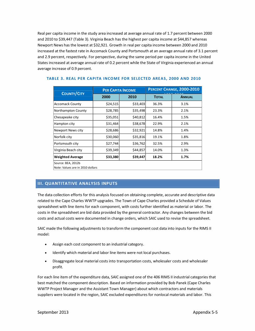
Real per capita income in the study area increased at average annual rate of 1.7 percent between 2000 and 2010 to $39,447 (Table 3). Virginia Beach has the highest per capita income at $44,857 whereas Newport News has the lowest at $32,921. Growth in real per capita income between 2000 and 2010 increased at the fastest rate in Accomack County and Portsmouth at an average annual rate of 3.1 percent and 2.9 percent, respectively. For perspective, during the same period per capita income in the United States increased at average annual rate of 0.2 percent while the State of Virginia experienced an annual average increase of 0.9 percent.
TAB LE 3. REAL PER CAPITA INCOME FOR SE LEC TED ARE AS, 2000 AND 2010
COUNTY/CITY PER CAPITA INCOME PERCENT CHANGE, 2000-2010
1990 2002 2000 2010 TOTAL ANNUAL
Accomack County $24,515 $33,403 36.3% 3.1%
Northampton County $28,785 $35,498 23.3% 2.1%
Chesapeake city $35,051 $40,812 16.4% 1.5%
Hampton city $31,464 $38,678 22.9% 2.1%
Newport News city $28,686 $32,921 14.8% 1.4%
Norfolk city $30,060 $35,816 19.1% 1.8%
Portsmouth city $27,744 $36,762 32.5% 2.9%
Virginia Beach city $39,349 $44,857 14.0% 1.3%
Weighted Average $33,380 $39,447 18.2% 1.7%
Source: BEA, 2012b Note: Values are in 2010 dollars
III. QUANTITATIVE ANALYSIS INPUTS
The data collection efforts for this analysis focused on obtaining complete, accurate and descriptive data related to the Cape Charles WWTP upgrades. The Town of Cape Charles provided a Schedule of Values spreadsheet with line items for each component, with costs further identified as material or labor. The costs in the spreadsheet are bid data provided by the general contractor. Any changes between the bid costs and actual costs were documented in change orders, which SAIC used to revise the spreadsheet.
SAIC made the following adjustments to transform the component cost data into inputs for the RIMS II model:
• Assign each cost component to an industrial category.
• Identify which material and labor line items were not local purchases.
• Disaggregate local material costs into transportation costs, wholesaler costs and wholesaler profit.
For each line item of the expenditure data, SAIC assigned one of the 406 RIMS II industrial categories that best matched the component description. Based on information provided by Bob Panek (Cape Charles WWTP Project Manager and the Assistant Town Manager) about which contractors and materials suppliers were located in the region, SAIC excluded expenditures for nonlocal materials and labor. This
September 2013 Appendix 5-5

adjustment is necessary because materials provided by vendors outside the region (e.g., membranes) represent leakage of dollars that are spent outside of the study region. Finally, SAIC used National Income and Product Accounts (NIPA) data to disaggregate expenditures on materials (i.e., purchaser cost) into cost components for wholesaler value, wholesaler markup and transportation costs.
Table 4 displays the total expenditures for the WWTP upgrade project. The original contract specified $14,737,000 with an additional $425,491 in change orders for a total amount of $15,162,491. Of the total amount, $10,823,056 was used to purchase materials, $3,850,435 went to labor costs and $489,000 was applied to insurance, bonding and mobilization. Not all of the purchases were made locally, with an estimated $5,196,972 spent outside of the study region. The amount that is input into the model to calculate the multiplier effects is $9,965,519.
TAB LE 4. TOTAL E XPE ND ITURE S FOR WWTP UPGR ADE
AMOUNT INPUT INTO MODEL
LEAKAGE, SAVINGS AND OTHER NON-INPUTS
Wholesale Purchases (includes transportation costs)
$10,823,056 $6,115,084 $4,707,972
Household Income (labor) $3,850,435 3,850,435 $0
Other $489,000 $0 $489,000
Total $15,162,491 $9,965,519 $5,196,972
IV. REGIONAL ECONOMIC IMPACTS
The regional economic impacts measure the increase in total economic output for the study region as a result of the Cape Charles WWTP upgrades. For the study region, the total economic output increased by $29,843,832. The total project value is $15,162,491 and the indirect and induced impacts are a combined $14,681,341, which implies a total impact-to-project value ratio of 1.97:1 (i.e., each dollar spent on the project resulted in a regional economic impact of approximately $1.97 including the initial expenditures and the indirect and induced demand changes). The region applied in this analysis represents the area where the expenditures and labor were procured. However, many of the materials used in the project were manufactured outside of the region. The smaller study region most likely results in a lower total impact-to-project value ratio because spending leakages are likely given the size of the local economy.
The multipliers vary by industry with the transportation and warehousing sector having the highest at 1.97 and the households sector having the lowest at 1.09 (Table 5). A higher multiplier indicates that direct expenditures on the products of that industry have a higher tendency to cycle throughout the regional economy multiple times via input-output linkages in local industries. The households multiplier of 1.09 indicates that household expenditures are more likely to leak outside the regional economy because of purchases of goods that are manufactured elsewhere and services purchased from suppliers outside the region. In addition, the household multiplier reflects leakages in the form of taxes and savings.
September 2013 Appendix 5-6

TAB LE 5. TOTAL OUTPUT BY IND USTRY B ASED ON R IMSII ANALY SIS
INDUSTRIAL SECTOR REGIONAL PURCHASES MULTIPLIER OUTPUT
IMPACTS Agriculture, Fishing and Hunting $48,059 1.57 $75,506
Mining $157,549 1.72 $271,013
Utilities $1,000 1.80 $1,797
Construction $249,642 1.92 $478,988
Manufacturing $4,455,431 1.67 $7,441,813
Wholesale Trade $607,532 1.72 $1,045,137
Transportation and Warehousing $361,871 1.97 $713,053
Professional and Technical Services $234,000 1.88 $439,733
Households $3,850,435 1.09 $4,214,301
Indirect and Induced Impacts $14,681,341
Total Project Value (including direct impact) $15,162,491
Total Output Impact $29,843,832
Note: Values are in 2008 dollars
Table 6 displays the total output attributable to ARRA funding. It is not known which items were purchased with the ARRA funding. The simplifying assumption had to be applied that the ARRA-funded proportion of the total project was spent in the same proportions as the non-ARRA funded portion. The ARRA funding on the project results in an increase in total output of $11,959,866.
TAB LE 6. TOTAL OUTPUT ATTR IB UTABLE TO ARR A FUND ING BASE D ON R IMSII ANALYSIS
Total Output
DIRECT
$6,076,343
INDIRECT AND INDUCED
$5,883,523
TOTAL OUTPUT
$11,959,866
Note: Values are in 2008 dollars
IV. OTHER ENVIRONMENTAL AND ECONOMIC BENEFITS
Water quality throughout the Chesapeake Bay watershed is impaired because excess nutrients and sediment loadings adversely affect the fish, shellfish and plants that are indigenous to the Bay. For example, nutrients cause algae blooms that deplete dissolved oxygen levels, block sunlight needed by underwater grasses, and smother aquatic life on the bottom (EPA, 2010).
Among the many sources of nutrient loadings are numerous WWTPs that discharge to various waterways throughout the Bay’s 64,000-square mile watershed. The Cape Charles WWTP is one of these sources. It has a National Pollutant Discharge Elimination System (NPDES) permit that limits the amount of contaminants such as nutrients that it can discharge to the Bay in its treated sewage flows.
September 2013 Appendix 5-7

A recent Chesapeake Bay TMDL establishes nutrient and sediment waste load allocations to help restore water quality. By 2025, the TMDL should reduce loadings of nitrogen by 25 percent and phosphorus loadings by 24 percent (EPA, 2010). The wasteload allocations for Virginia’s portion of the Eastern Shore are 1.31 million pounds per year for nitrogen, 0.14 million pounds per year for phosphorus, and 11.31 million pounds per year for sediment (EPA, 2010). These loads are further allocated among point sources such as WWTPs and nonpoint sources such as runoff from agricultural areas.
Cropper and Isaac (2011) identify the following types of use-related benefits of achieving the water quality standards in the Chesapeake Bay5:
• Commercial and recreational fishery benefits of improved fish and shellfish stocks.
• Boater and swimmer recreational benefits of improved water clarity.
• Property value increases of improved aesthetic and recreational values.
They also identify nonuse benefits in the form of higher existence values for improved water quality (i.e., higher willingness-to-pay for water quality improvements because people place intrinsic value on the quality of water resources). There are, however, no quantitative benefit estimates for the TMDL.
In addition to providing environmental benefits associated with reduced nutrient loadings, the WWTP upgrades should provide medium and long-term benefits to the Town of Cape Charles by increasing economic growth potential. The upgrades will allow water reuse for nonpotable use such as golf course irrigation and process water for a concrete supplier (Town of Cape Charles, 2009). This reuse capability reduces the current WWTP discharge volume to the Bay as well as aquifer withdrawals (Town of Cape Charles, 2009). Furthermore, the excess discharge capacity under the NPDES permit remains available to accommodate future population growth and related economic development (Panek, 2012).
5 Categories of benefits can be divided into those associated with resource use and those that do not require direct or indirect resource use. Use-related benefits categories include human health benefits such as reduced risk of mortality or morbidity; resource use for commercial purposes; resource use for recreational purposes or aesthetic enjoyment; and indirect resource use via its support for ecosystem functions. Nonuse benefits arise when natural resources or environmental quality have intrinsic value aside from their ability to directly or indirectly provide goods and services.
September 2013 Appendix 5-8

REFERENCES
Bureau of Economic Analysis (BEA). 2012a. Data from U.S. Census Bureau accessed on BEA website on May 14, 2012. http://www.bea.gov/regional/
BEA. 2012b. "Decennial Census, 2000 and 2010”. "Local Area Personal Income & Employment" Interactive tables on website. Accessed May 14, 2012. http://www.bea.gov/regional/
BEA. 2012c. RIMS II: An essential tool for regional developers and planners. Washington, D.C.; U.S. Government Printing Office.
BEA. 2012d. RIMS II Multipliers 2002/2008: Table 1.5, Total Multipliers for Output by Detailed Industry, Custom Study Region (Type II). May 2012.
Cropper, M.L., and W.S. Isaac. 2011. “The Benefits of Achieving the Chesapeake Bay TMDLs (Total Maximum Daily Loads): A Scoping Study.” RFF Discussion Paper 11-31. Available online at http://www.rff.org/RFF/Documents/RFF-DP-11-31.pdf.
EPA. 2000. Brownfields Assessment Demonstration Pilot: Cape Charles-Northampton County, VA. EPA 500-F-00-261.
EPA. 2010. The Chesapeake Bay TMDL. Available online at http://www.epa.gov/reg3wapd/tmdl/ChesapeakeBay/tmdlexec.html.
Panek, Bob. 2012. Personal communication with Walter Gills (VA DEQ), Kelly Ward (VA DEQ), Ed Hopkins (EPA/R3), Hamilton Humes (EPA/OCFO), and SAIC staff. May 8, 2012.
Town of Cape Charles. 2009. “Cape Charles WWTP Nutrient Removal Upgrade Groundbreaking Ceremony – November 12, 2009.” Electronic file: Groundbreaking Handout.pdf
September 2013 Appendix 5-9

This page intentionally blank.
September 2013 Appendix 5-10

APPENDIX 6: CITY OF HEDRICK WASTEWATER TREATMENT PLANT UPGRADES

This page intentionally blank.

I. PROJECT DESCRIPTION
The City of Hedrick is located in Keokuk County, Iowa, which is about 90 miles southwest of the City of Cedar Rapids. The project area consists of eight counties in southeastern Iowa, two of which are within the Cedar Rapids, IA metropolitan statistical area (MSA).
In 2009, the City of Hedrick received $2.3 million to support the planning, design and construction for a new $4.6 million wastewater treatment facility. The SRF funding of $2.3 million included an ARRA loan of $899,000 with 100% principal forgiveness.
The project consisted of replacing the wastewater lift station with one of greater capacity and constructing a new wastewater treatment facility. The increased capacity in lift station is expected to eliminate uncontrolled discharges during heavy rain events. The wastewater treatment system will include an Aeromod activated sludge plant to allow for larger flows and effective removal of ammonia from the wastewater before discharge into stream resulting in a higher quality effluent being introduced to receiving stream. The treatment plant will also employ reed bed technology for sludge storage (State of Iowa, 2012). This goal of the project was to maximize job creation and economic benefit by investing in infrastructure that provides long-term economic benefits to the community while avoiding reductions in essential services.
II. REGION DESCRIPTION
The study region (Figure 1) consists of eight counties in southeastern Iowa, two of which are within the Cedar Rapids, IA MSA. The City of Hedrick is located in Keokuk County about 90 miles southwest of the City of Cedar Rapids, which is located in Linn County. The market area reaches the Illinois boundary, but only includes counties within the State of Iowa to remain consistent with the economically independent defined MSA.
September 2013 Appendix 6-1

F IGURE 1. H EDR IC K WWTP EC ONOMIC IMPAC T STUDY REGION
September 2013 Appendix 6-2

The study region includes the following counties within the State of Iowa: Benton, Iowa, Johnson, Keokuk, Linn, Louisa, Muscatine and Washington.
POPULATION
Table 1 reports population data for the study region components. In aggregate, the population in the communities within the study area increased 9.4 percent between 2000 and 2010 largely driven by the growth in Johnson and Linn counties, which increased by 17.7 percent and 10 percent respectively. Population declined in Keokuk and Louisa counties and increased modestly in the remaining four counties.
TAB LE 1. POPULATION CH ANGE S IN SELE CTED ARE AS, 2000- 2010
COUNTY POPULATION PERCENT CHANGE, 2000-2010
2000 2010 TOTAL ANNUAL
Benton, IA 25,326 26,073 2.9% 0.3%
Iowa, IA 15,729 16,338 3.9% 0.4%
Johnson, IA 111,455 131,238 17.7% 1.6%
Keokuk, IA 11,418 10,501 -8.0% -0.8%
Linn, IA 192,365 211,564 10.0% 1.0%
Louisa, IA 12,174 11,374 -6.6% -0.7%
Muscatine, IA 41,791 42,732 2.3% 0.2%
Washington, IA 20,718 21,712 4.8% 0.5%
Total 430,976 471,532 9.4% 0.9% Source: BEA, 2012a
LOCAL ECONOMY
Within the study region, local and state government is a significant portion of the full- and part-time employment accounting for 15.8 percent of total employment, up from 15.0 percent in 2001 (Table 2). Next, manufacturing and retail trade account for 11.7 percent and 10.5 percent of employment, respectively. The manufacturing sector experienced the largest decline with over 4,200 fewer employees in this sector and a loss of over 2.2% in the share of total employment. The health care and social assistance sector experienced the largest increase with over 8,200 new employees and a 2.1% gain in the share of total employment.
September 2013 Appendix 6-3

TAB LE 2. E MPLOY ME NT BY IND USTR IAL SE CTOR , 2001 AND 2010
INDUSTRIAL SECTOR 2001 2010 PERCENT OF TOTAL 2001 2010
Total Employment 306,462 326,793 100% 100%
Farm Employment 9,997 8,519 3.3% 2.6%
Forestry, Fishing and Hunting 185 183 0.1% 0.1%
Mining 74 191 0.0% 0.1%
Utilities 1,552 1,878 0.5% 0.6%
Construction 16,611 16,381 5.4% 5.0%
Manufacturing 42,554 38,288 13.9% 11.7%
Wholesale Trade 8,961 8,365 2.9% 2.6%
Retail Trade 35,013 34,202 11.4% 10.5%
Transportation and Warehousing 10,567 13,807 3.4% 4.2%
Information 10,936 8,378 3.6% 2.6%
Finance and Insurance 12,225 16,734 4.0% 5.1%
Real Estate, Rental and Leasing 8,239 9,941 2.7% 3.0%
Professional and Technical Services 10,100 12,486 3.3% 3.8%
Management of Companies 372 1,369 0.1% 0.4%
Administrative and Waste Services 15,834 15,835 5.2% 4.8%
Educational Services 5,828 7,547 1.9% 2.3%
Health Care and Social Assistance 21,490 29,702 7.0% 9.1%
Arts, Entertainment and Recreation 4,340 5,343 1.4% 1.6%
Accommodation and Food Services 17,892 20,383 5.8% 6.2%
Other Services 14,185 14,438 4.6% 4.4%
Federal Government, Civilian 3,194 3,363 1.0% 1.0%
Military 2,022 2,001 0.7% 0.6%
State and Local Government 45,901 51,623 15.0% 15.8% Source: BEA, 2012b Note: Totals include employment that is not displayed in the sector breakout because of non-disclosure issues.
September 2013 Appendix 6-4

Real per capita income in the study area increased at average annual rate of 2.4 percent between 2000 and 2010 to $39,514 (Table 3). Linn has the highest per capita income at $41,062 whereas Louisa has the lowest at $32,197. Growth in per capita income between 2000 and 2010 increased at the fastest rate in Benton County at average annual rate of 1.2 percent with the other counties increasing between 0.2 and 0.7 percent except for Linn, which was essentially flat, and Iowa County, which experienced a small decrease. For perspective, during the same period per capita income in the United States increased at average annual rate of 0.2 percent while the State of Iowa experienced an annual average increase of 0.8 percent.
TAB LE 3. REAL PER CAPITA INCOME FOR SE LEC TED ARE AS, 2000 AND 2010
COUNTY/CITY PER CAPITA INCOME PERCENT CHANGE, 2000-2010 2000 2010 TOTAL ANNUAL
Benton, IA $34,681 $39,066 12.6% 1.2%
Iowa, IA $38,798 $37,797 -2.6% -0.3%
Johnson, IA $38,890 $39,607 1.8% 0.2%
Keokuk ,IA $30,713 $32,770 6.7% 0.7%
Linn, IA $40,891 $41,062 0.4% 0.0%
Louisa, IA $30,733 $32,197 4.8% 0.5%
Muscatine, IA $33,857 $36,100 6.6% 0.6%
Weighted Average $38,583 $39,514 2.4% 0.2%
Source: BEA, 2012b Note: Values are in 2010 dollars
III. QUANTITATIVE ANALYSIS INPUTS
The data collection efforts for this analysis focused on obtaining complete, accurate and descriptive data related to the Hedrick WWTP construction project. The Iowa SRF provided several scanned cost sheets with line items for each component. The costs in the cost sheets are bid data provided by the general contractor. Any changes between the bid costs and actual costs were documented in change orders, which SAIC used to revise the original cost data.
SAIC made the following adjustments to transform the component cost data into inputs for the RIMS II model:
• Assign each cost component to an industrial category.
• Split item costs into material and labor categories.
• Identify which material and labor line items were not local purchases.
• Disaggregate local material costs into transportation costs, wholesaler costs and wholesaler profit.
For each line item of the expenditure data, SAIC assigned one of the 406 RIMS II industrial categories that best matched the component description. SAIC excluded expenditures for nonlocal materials and labor using information in the provided cost sheets. Where the source of purchase was not readily identified,
September 2013 Appendix 6-5

SAIC applied Census County Business Patterns data to determine whether there were businesses within the study region that could supply the item in question. This adjustment is necessary because materials provided by vendors outside the region (e.g., filtration package plant) represent leakage of dollars that are spent outside of the study region. Finally, SAIC used National Income and Product Accounts (NIPA) data to disaggregate expenditures on materials (i.e., purchaser cost) into cost components for wholesaler value, wholesaler markup and transportation costs.
Table 4 displays the enumerated expenditures for the WWTP upgrade project. The total contract amounts to $3,356,043 including change orders. ARRA funding accounted for about 27 percent of the value of the project with $899,000 provided in the form of a principal-forgiven loan. Of the total amount, $2,665,016 was used to purchase materials, $636,027 went to labor costs, and $55,000 was applied to insurance, bonding and mobilization. Not all of the purchases were made locally, with an estimated $1,233,424 spent outside of the study region. The amount that is input into the model to calculate the multiplier effects is $2,122,619
TAB LE 4. TOTAL E XPE ND ITURE S FOR WWTP CONSTR UCTION
AMOUNT INPUT INTO MODEL
LEAKAGE, SAVINGS AND OTHER NON-INPUTS
Wholesale Purchases (includes transportation costs)
$2,665,016 $1,486,592 $1,178,424
Household Income (labor) $636,027 $636,027 $0
Other $55,000 $0 $55,000
Total $3,356,043 $2,122,619 $1,233,424
Note: Values are in 2008 dollars
IV. REGIONAL ECONOMIC IMPACTS
The regional economic impacts measure the increase in total economic output for the study region as a result of the Cape Charles WWTP upgrades. For the study region, the total economic output increased by $6,339,383. The total project value is $3,356,043 and the indirect and induced impacts are a combined $2,983,340, which implies a total impact-to-project value ratio of 1.89:1 (i.e., each dollar spent on the project resulted in a regional economic impact of approximately $1.89 including the initial expenditures and the indirect and induced demand changes). The region applied in this analysis represents the area where the expenditures and labor were procured. However, many of the materials used in the project were manufactured outside of the region. The smaller study region most likely results in a lower total impact-to-project value ratio because spending leakages are likely given the size of the local economy.
The multipliers vary by industry with the construction sector having the highest at 1.77 and the households sector having the lowest at 0.88 (Table 5). A higher multiplier indicates that direct expenditures on the products of that industry have a higher tendency to cycle throughout the regional economy multiple times via input-output linkages in local industries. The household multiplier of 0.88 indicates that household expenditures are more likely to leak outside the regional economy because of purchases of goods that are manufactured elsewhere and services purchased from suppliers outside the region. In addition, the households multiplier reflects leakages in the form of taxes and savings.
September 2013 Appendix 6-6

TAB LE 5. TOTAL OUTPUT BY IND USTRY B ASED ON R IMSII ANALY SIS
INDUSTRIAL SECTOR REGIONAL PURCHASES MULTIPLIER OUTPUT
IMPACTS Agriculture, Fishing and Hunting $4,997 1.50 $7,489
Mining $2,165 1.62 $3,503
Construction $200,062 1.77 $354,651
Manufacturing $1,082,715 1.61 $1,747,003
Wholesale Trade $135,403 1.54 $207,925
Transportation and Warehousing $57,968 1.74 $100,888
Professional and Technical Services $3,281 1.61 $5,294
Households $636,027 0.88 $556,587
Indirect and Induced Impacts $2,983,340
Total Project Value (including direct impact) $3,356,043
Total Output Impact $6,339,383
Note: Values are in 2008 dollars
Table 6 displays the total output attributable to ARRA funding. It is not known which items were purchased with the ARRA funding. The simplifying assumption had to be applied that the ARRA-funded proportion of the total project was spent in the same proportions as the non-ARRA funded portion. The ARRA funding on the project results in an increase in total output of $1,698,162.
TAB LE 6. TOTAL OUTPUT ATTR IB UTABLE TO ARR A FUND ING BASE D ON R IMSII ANALYSIS
DIRECT INDIRECT AND INDUCED TOTAL OUTPUT
Total Output $899,000 $799,162 $1,698,162
Note: Values are in 2008 dollars
V. OTHER ENVIRONMENTAL AND ECONOMIC BENEFITS
The Hedrick treatment plant project includes constructing a new treatment facility that includes an activated sludge plant, headworks, pumping stations, reed beds and a new lift station adjacent to the plant to replace an existing lift station (Krewson, 2009). The new plant has a design capacity of 1.878 million gallons per day (MGD; peak hour wet weather flow) and average flows of 0.465 MGD (wet weather) and 0.103 (dry weather) (Leopold, 2009). The plant was designed to meet national pollution discharge elimination system (NPDES) permit limits for ammonia, biological oxygen demand, total suspended solids and bacteria. These upgrades will improve the wastewater utility’s effluent quality and reduce loadings of nutrients and sediments in the receiving waters.
One of the green components of the project is using reed beds for sludge dewatering instead of more conventional options such as drying pads. Although there is no performance data available for the Hedrick facility, a study of another site shows that reed beds have the potential to dewater a greater volume of sludge per square foot of drying area, which reduces the land area needed for sludge drying (NYSERDA,
September 2013 Appendix 6-7

2006). The plants in a reed bed dewater sludge via water uptake, which is more efficient than dewatering via evaporation on a drying pad. The reed bed in a demonstration project achieved a 78% reduction in sludge volume compared to a 60% reduction for a drying bed (NYSERDA 2008). The reed bed also allows a higher loading rate per square foot of drying area and extended sludge storage. The same demonstration site showed that a reed bed could reduce annualized operating costs for sludge handling by over 70% because the sludge can remain in the reed bed for up to 10 years, but drying pads incur annual costs for sludge cake removal and disposal (NYSERDA, 2008). In addition, the plants may remove some contaminants such as metals.
The financial subsidies will benefit the utility’s customers. Of the total project, only $1.6 million will need to be repaid. Although the utility raised rates to repay the 20-year loan, the fee increases would have been substantially higher if the full amount had been financed via loans or bonds. The base household fee increased from $12.45 to $27.50, and the usage fees per 1,000 gallons over 3,000 per month increased from $4.15 to $5.30 (Davis, 2011). The principal forgiveness provision of the ARRA funding contributed to the affordability of the plant upgrades.
REFERENCES
Bureau of Economic Analysis (BEA). 2012a. Data from U.S. Census Bureau accessed on BEA website on September 7, 2012. http://www.bea.gov/regional/
BEA. 2012b. "Decennial Census, 2000 and 2010”. "Local Area Personal Income & Employment" Interactive tables on website. Accessed May 14, 2012. http://www.bea.gov/regional/
BEA. 2012c. RIMS II: An essential tool for regional developers and planners. Washington, D.C.; U.S. Government Printing Office.
BEA. 2012d. RIMS II Multipliers 2002/2008: Table 1.5, Total Multipliers for Output by Detailed Industry, Custom Study Region (Type II). September 2012.
Davis, C. 2011. “Hedrick Shoulders Sewer Rate Hikes.” Ottumwa Courier Online. October 25, 2011.
Krewson, J. 2009. Iowa State Revolving Fund - Categorical Exclusion. Prepared by Iowa Department of Natural Resources.
Leopold, R. 2009. Construction Permit. Prepared by Iowa Department of Natural Resources.
New York State Energy Research and Development Authority (NYSERDA). 2006. Energy Efficient Sludge Treatment with Reed-Bed Technology Demonstration Project. Final Report 06-12.
State of Iowa - Reporting on Iowa's Economic Recovery. https://reporting.iowa.gov/?cmd=AwardReports&AwardID=09-CDR-002. Accessed September 27, 2012.
U.S. Census Bureau. County Business Patterns, 2010 for Benton, Iowa, Johnson, Keokuk, Linn, Louisa, Muscatine and Washington counties
September 2013 Appendix 6-8

APPENDIX 7: GRANT COUNTY SANITARY SEWER DISTRICT EXTENSION

This page intentionally blank.
I. PROJECT DESCRIPTION
Grant County is located in northern Kentucky with the county seat in the City of Williamstown about 46 miles north of the City of Lexington. The project area consists of eight counties in northern Kentucky, six of which are within the Lexington-Fayette, KY metropolitan statistical area (MSA).
In 2010, the Grant County Sanitary Sewer District received $300,000 in ARRA funding to support the planning, design and construction for phase 1 of the extension to the County’s sanitary sewer, which cost approximately $1.9 million. Of the total ARRA loan of $300,000, principal forgiveness amounted to $156,300; the remainder is a loan to be repaid over 20 years at 3% interest.
The project extended sanitary sewer service to 50 residential customers and two larger customers who operated their own sewage package plants: a commercial campground that had a functioning plant, but was beginning to have problems; and a mobile home park (MHP) that had an old package plant that was not meeting National Pollutant Discharge Elimination System (NPDES) permit limits. It also reaches a second MHP that has not tied in yet. According to the design engineer for the project, Kerry Odle, the existing sewer treatment plant has excess capacity, so the added wastestream does not affect the plant (Odle, 2012).
II. REGION DESCRIPTION
The study region (Figure 1) consists of eight counties in northern Kentucky, six of which are within the Lexington-Fayette, KY MSA. The market area reaches both the Indiana and Ohio borders, but only includes counties within the State of Kentucky to remain consistent with the economically independent defined MSA. Kerry Odle, the Project Engineer, confirmed that materials were purchased from the Lexington-Fayette, KY MSA rather than the Cincinnati, OH MSA. The study region includes the following counties within the State of Kentucky: Boone, Bourbon, Clark, Fayette, Grant, Jessamine, Scott and Woodford.
September 2013 Appendix 7-1

F IGURE 1. GRANT C OUNTY SANITARY SEWER EC ONOMIC IMPAC T STUDY REGION
September 2013 Appendix 7-2
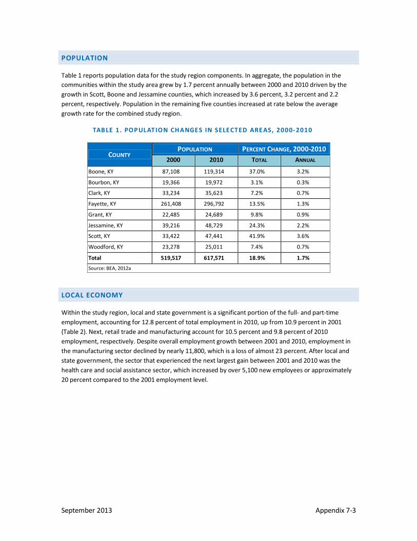
POPULATION
Table 1 reports population data for the study region components. In aggregate, the population in the communities within the study area grew by 1.7 percent annually between 2000 and 2010 driven by the growth in Scott, Boone and Jessamine counties, which increased by 3.6 percent, 3.2 percent and 2.2 percent, respectively. Population in the remaining five counties increased at rate below the average growth rate for the combined study region.
TAB LE 1. POPULATION CH ANGE S IN SELE CTED ARE AS, 2000- 2010
COUNTY POPULATION PERCENT CHANGE, 2000-2010
2000 2010 TOTAL ANNUAL
Boone, KY 87,108 119,314 37.0% 3.2%
Bourbon, KY 19,366 19,972 3.1% 0.3%
Clark, KY 33,234 35,623 7.2% 0.7%
Fayette, KY 261,408 296,792 13.5% 1.3%
Grant, KY 22,485 24,689 9.8% 0.9%
Jessamine, KY 39,216 48,729 24.3% 2.2%
Scott, KY 33,422 47,441 41.9% 3.6%
Woodford, KY 23,278 25,011 7.4% 0.7%
Total 519,517 617,571 18.9% 1.7%
Source: BEA, 2012a
LOCAL ECONOMY
Within the study region, local and state government is a significant portion of the full- and part-time employment, accounting for 12.8 percent of total employment in 2010, up from 10.9 percent in 2001 (Table 2). Next, retail trade and manufacturing account for 10.5 percent and 9.8 percent of 2010 employment, respectively. Despite overall employment growth between 2001 and 2010, employment in the manufacturing sector declined by nearly 11,800, which is a loss of almost 23 percent. After local and state government, the sector that experienced the next largest gain between 2001 and 2010 was the health care and social assistance sector, which increased by over 5,100 new employees or approximately 20 percent compared to the 2001 employment level.
September 2013 Appendix 7-3

TAB LE 2. E MPLOY ME NT BY IND USTR IAL SE CTOR , 2001 AND 2010
INDUSTRIAL SECTOR 2001 2010 PERCENT OF TOTAL 2001 2010
Total Employment 386,295 409,599 100.0% 100.0%
Farm Employment 12,103 10,049 3.1% 2.5%
Forestry, Fishing and Hunting 1,923 1,934 0.5% 0.5%
Mining 411 392 0.1% 0.1%
Utilities 1,222 609 0.3% 0.1%
Construction 22,803 18,221 5.9% 4.4%
Manufacturing 51,997 40,200 13.5% 9.8%
Wholesale Trade 14,585 16,712 3.8% 4.1%
Retail Trade 44,899 43,086 11.6% 10.5%
Transportation and Warehousing 21,334 20,913 5.5% 5.1%
Information 8,131 7,052 2.1% 1.7%
Finance and Insurance 13,695 16,086 3.5% 3.9%
Real Estate, Rental and Leasing 11,397 15,747 3.0% 3.8%
Professional and Technical Services 17,837 21,717 4.6% 5.3%
Management of Companies 3,057 4,484 0.8% 1.1%
Administrative and Waste Services 20,166 24,547 5.2% 6.0%
Educational Services 4,124 7,521 1.1% 1.8%
Health Care and Social Assistance 25,390 30,522 6.6% 7.5%
Arts, Entertainment and Recreation 6,668 8,973 1.7% 2.2%
Accommodation and Food Services 26,701 30,632 6.9% 7.5%
Other Services 16,820 19,108 4.4% 4.7%
Federal Government, Civilian 5,502 6,175 1.4% 1.5%
Military 1,760 2,046 0.5% 0.5%
State and Local Government 42,200 52,337 10.9% 12.8% Source: BEA, 2012b Note: Totals include employment that is not displayed in the sector breakout because of non-disclosure issues.
September 2013 Appendix 7-4

Real per capita income in the study area decreased at average annual rate of 1.0 percent between 2000 and 2010 to $35,098 as wages failed to keep pace with inflation primarily due the loss of higher-paying manufacturing jobs (Table 3). The variation in per capita incomes among counties within the study region is substantial with Woodford having the highest 2010 real per capita income of $40,483 and Grant having the lowest of $28,058. The rate of decline in real per capita income between 2000 and 2010 was fastest in Bourbon County, where per capita income declined at average annual rate of 2.2 percent. Other counties experienced declines ranging between 0.1 and 1.6 percent per year. For perspective, during the same period per capita income in the United States increased at average annual rate of 0.2 percent while the State of Kentucky experienced an annual average increase of 0.2 percent.
TAB LE 3. REAL PER CAPITA INCOME FOR SE LEC TED ARE AS, 2000 AND 2010
COUNTY/CITY PER CAPITA INCOME PERCENT CHANGE, 2000-2010 2000 2010 TOTAL ANNUAL
Boone, KY $39,215 $34,043 -13.2% -1.4%
Bourbon, KY $38,428 $30,903 -19.6% -2.2%
Clark, KY $34,590 $32,697 -5.5% -0.6%
Fayette, KY $40,514 $37,874 -6.5% -0.7%
Grant, KY $28,244 $28,058 -0.7% -0.1%
Jessamine, KY $33,594 $29,863 -11.1% -1.2%
Scott, KY $38,717 $32,995 -14.8% -1.6%
Woodford, KY $46,977 $40,483 -13.8% -1.5%
Weighted Average $38,960 $35,098 -9.9% -1.0% Source: BEA, 2012b Note: Values are in 2010 dollars
III. QUANTITATIVE ANALYSIS INPUTS
The data collection efforts for this analysis focused on obtaining complete, accurate and descriptive data related to the Grant County sanitary sewer construction project. The Kentucky Infrastructure Authority provided two detailed spreadsheets with line items for each component and information regarding the location and payrolls of the contractors. The costs in the cost sheets are bid data provided by the general contractor. Any changes between the bid costs and actual costs were documented in change orders, which SAIC used to revise the original cost data.
SAIC made the following adjustments to transform the component cost data into inputs for the RIMS II model:
• Assign each cost component to an industrial category.
• Split item costs into material and labor categories.
• Identify which material and labor line items were not local purchases.
• Disaggregate local material costs into transportation costs, wholesaler costs and wholesaler profit.
September 2013 Appendix 7-5

For each line item of the expenditure data, SAIC assigned one of the 406 RIMS II industrial categories that best matched the component description. SAIC excluded expenditures for nonlocal materials and labor using information in the provided cost sheets. Where the source of purchase was not readily identified, SAIC applied Census County Business Patterns (U.S. Census Bureau, 2010) data to determine whether there were businesses within the study region that could supply the item in question. This adjustment is necessary because materials provided by vendors outside the region (e.g., filtration package plant) represent leakage of dollars that are spent outside of the study region. Finally, SAIC used National Income and Product Accounts (NIPA) data to disaggregate expenditures on materials (i.e., purchaser cost) into cost components for wholesaler value, wholesaler markup and transportation costs.
Table 4 displays the total expenditures for the sanitary sewer construction project. The total contract was $1,933,558. ARRA funding of $300,000 accounted for about 15.5 percent of the value of the project and included principal forgiveness for $156,300; the remainder is a loan to be repaid over 20 years at 3% interest. Of the total contract amount, $1,532,459 was used to purchase materials and $401,100 went to labor. Not all of the purchases were made locally, with an estimated $110,000 spent outside of the study region. The amount that is input into the model to calculate the multiplier effects is $1,823,558.
TAB LE 4. TOTAL E XPE ND ITURE S FOR SANITARY SE WER C ONSTR UC TION
AMOUNT INPUT INTO MODEL
LEAKAGE, SAVINGS AND OTHER NON-INPUTS
Wholesale Purchases (includes transportation costs)
$1,532,459 $1,422,459 $110,000
Household Income (labor) $401,100 $401,100 $0
Total $1,933,558 $1,823,558 $110,000
Note: Values are in 2010 dollars
IV. REGIONAL ECONOMIC IMPACT
The regional economic impacts measure the increase in total economic output for the study region as a result of the Grant County sanitary sewer construction spending (BEA, 2012c). For the study region, the total economic output increased by $4,847,230. The total project value is $1,933,558 and the indirect and induced impacts are a combined $2,913,671, which implies a total impact-to-project value ratio of 2.51:1 (i.e., each dollar spent on the project resulted in a regional economic impact of approximately $2.51 including the initial expenditures and the indirect and induced demand changes). The region applied in this analysis represents the area where the expenditures and labor were procured. If, however, workers living in the northern counties (Boone and Grant) tend to spend earnings in the Cincinnati, OH MSA instead of the Lexington-Fayette, KY MSA, then the households multiplier may overstate the impact of some portion of the household earnings portion of total project expenditures.
The multipliers vary by industry with the transportation and warehousing sector having the highest at 1.89 and the households sector having the lowest at 1.02 (Table 5). A higher multiplier indicates that direct expenditures on the products of that industry have a higher tendency to cycle throughout the regional economy multiple times via input-output linkages in local industries. The households multiplier of 1.02 indicates that household expenditures are more likely to leak outside the regional economy because
September 2013 Appendix 7-6

of purchases of goods that are manufactured elsewhere and services purchased from suppliers outside the region. In addition, the households multiplier reflects leakages in the form of taxes and savings.
TAB LE 5. TOTAL OUTPUT BY IND USTRY B ASED ON R IMSII ANALY SIS
INDUSTRIAL SECTOR REGIONAL PURCHASES MULTIPLIER OUTPUT
IMPACTS Mining $4,396 1.71 $7,522
Construction $358,999 1.87 $671,651
Manufacturing $898,622 1.73 $1,552,419
Wholesale Trade $123,420 1.64 $202,470
Transportation and Warehousing $37,022 1.89 $69,845
Households $401,100 1.02 $409,764
Indirect and Induced Impacts $2,913,671
Total Project Value (including direct impact) $1,933,558
Total Output Impact $4,847,230
Note: Values are in 2010 dollars
Table 6 displays the total output attributable to ARRA funding. It is not known which items were purchased with the ARRA funding. The simplifying assumption had to be applied that the ARRA-funded proportion of the total project was spent in the same proportions as the non-ARRA funded portion. The ARRA funding on the project results in an increase in total output of $752,069.
TAB LE 6. TOTAL OUTPUT ATTR IB UTABLE TO ARR A FUND ING BASE D ON R IMSII ANALYSIS
DIRECT INDIRECT AND INDUCED TOTAL OUTPUT
Total Output $300,000 $452,069 $752,069
Note: Values are in 2010 dollars
V. OTHER ENVIRONMENTAL AND ECONOMIC BENEFITS
The Grant County Sanitary Sewer District (the District) provides sanitary sewer service to approximately 1,500 customers via approximately 30 miles of sewer lines. Its customers are primarily located in and around the city of Crittenden, KY. The District also operates a sanitary sewer treatment plant, which was operating at 60% of its maximum treatment capacity of 0.3 million gallons per day (MGD) (Grant County Sanitary Sewer District, 2010).
The project extended sanitary sewer service along the US-25 corridor between Crittenden and Dry Ridge. This sewer extension brings sanitary sewer service to the Grant Mobile Home Park and the Cincinnati South Campground recreational vehicle park, both of which operated package sewage treatment plants. It
September 2013 Appendix 7-7
also provides service to residences, businesses and churches that previously used septic systems. Furthermore, service will also be available to three additional mobile home parks serviced by package treatment plants, should they choose to connect to the sewer system. Finally, the US-25 corridor is believed to be the area with the greatest potential for growth and development in Grant County. Therefore, the project provides service for future development and growth (Grant County Sanitary Sewer District, 2010).
An immediate environmental benefit of the project comes from switching the Grant County Mobile Home Park (56 mobile home pads) and Cincinnati South Campground (12 acres in size) from package wastewater treatment plants to centralized treatment. The average daily flow from these plants is 17,000 gallons (Grant County Sanitary Sewer District, 2010). Although the campground’s plant is meeting its discharge permit limits, the mobile home park’s plant is older and is no longer meeting its permit limits for chlorine residual (Odle, 2012) and (EPA ECHO, 2012). Therefore, shifting treatment to the Grant County plant will improve surface water quality in the receiving streams for discharges from the two package plants. Although the connections will increase the flow of treated effluent from the District’s treatment plant, larger centralized treatment plants can have more advanced treatment capabilities compared to small package plants.
Another environmental benefit pertains to the new customers who switched from septic systems to the sewer service. The original grant proposal estimated that at least 15 of the replaced septic systems had failed. Untreated sewage from these systems may not affect ground water quality, but because of the clay soils, sewage can seep to the surface causing health risks and odor problems (Odle, 2012).
The future economic benefits will primarily be realized when growth occurs along the US-25 corridor. Investors in new commercial operations will have readily available sewer connections. A wood truss factory that closed during the recession now has sewer service, which may make the industrial site easier to sell. Among the medium-term benefits, the connecting campground and mobile home park avoid the costs of maintaining and replacing their own package treatment plants, which is likely to be more expensive than the sewer connection and service fees.
REFERENCES
Bureau of Economic Analysis (BEA). 2012a. Data from U.S. Census Bureau accessed on BEA website on November 9, 2012. http://www.bea.gov/regional/
BEA. 2012b. "Decennial Census, 2000 and 2010”. "Local Area Personal Income & Employment" Interactive tables on website. Accessed November 9, 2012. http://www.bea.gov/regional/
BEA. 2012c. RIMS II: An essential tool for regional developers and planners. Washington, D.C.; U.S. Government Printing Office.
BEA. 2012d. RIMS II Multipliers 2002/2010: Table 1.5, Total Multipliers for Output by Detailed Industry, Custom Study Region (Type II). October 2012.
September 2013 Appendix 7-8

EPA ECHO. 2012. Available online at http://www.epa-echo.gov/cgi-bin/effluents.cgi?permit=KY0083631&charts=viols&monlocn=all&outt=all accessed October 2012.
Grant County Sanitary Sewer District. 2010. Application of the Grant County Sanitary Sewer District for Certificate of Public Convenience and Necessity to Construct Proposed Sanitary Sewer Line Improvements and Approval of the Proposed Plan to Finance the Improvements. Available online at http://psc.ky.gov/pscscf/2009%20cases/2009-00488/20091210_grant_application.pdf accessed October 2012.
Odle, Kerry. 2012. Personal communication with SAIC. October 26, 2012.
U.S. Census Bureau. County Business Patterns, 2010 for Boone, Bourbon, Clark, Fayette, Grant, Jessamine, Scott and Woodford counties.
September 2013 Appendix 7-9

This page intentionally blank.
September 2013 Appendix 7-10

APPENDIX 8: SANTA CRUZ COUNTY REDUCTION OF NONPOINT SOURCE SEDIMENT AND PESTICIDE POLLUTION

This page intentionally blank.
I. PROJECT DESCRIPTION
Santa Cruz County is located along the California coastline about 73 miles south of the City of San Francisco. The County of Santa Cruz Department of Public Works (CSCDPW) utilized $226,089 in ARRA funding to partially finance activities under its integrated vegetation management plan (IVMP). The CSCDPW is responsible for maintaining 600 miles of roadway in the county. In addition to road construction and repair, the CSCDPW controls roadside vegetation to maintain good visibility along the roadways and reduce fire risk of either on-road vehicles or fire spread across roadways. Roadside vegetation is also a vector for the spread of invasive plants. Roadways managed by the CSCDPW have gravel pullouts that are subject to soil erosion. The CSCDPW adopted the IVMP to replace historical control and management measures such as pesticide application, frequent mowing and gravel addition with more sustainable practices.
According to Connie Silva of the CSCDPW, the ARRA funding replaced approximately $200,000 in expected State Water Resources Control Board (SWRCB) grant funds that could not be allocated to the County because of California’s fiscal crisis (Silva, 2012). The SWRCB supported the initial project phase, during which the IVMP was developed and partially implemented at top priority sites. The ARRA funding helped complete the IVMP project. The ARRA funding of $226,089 included 100 percent principal forgiveness.
II. REGION DESCRIPTION
Based on information provided by Connie Silva, the CSCDPW Project Manager, the project used materials from local nurseries and employed local labor increasing the benefits to the local community (Silva, 2012). Therefore, the study region (Figure 2) consists solely of Santa Cruz County. The main cities are Santa Cruz and Watsonville.
September 2013 Appendix 8-1

F IGURE 1. SANTA CR UZ VE GETAT ION MANAGE ME NT EC ONOMIC IMPAC T STUDY REG ION
September 2013 Appendix 8-2

POPULATION
Table 1 reports population and real per capita income data for the study region. The population within the study area grew by 0.3 percent annually between 2000 and 2010. Real per capita income growth decreased at an average annual rate of 1.2 percent between 2000 and 2010 from $52,611 to $46,586. For perspective, during the same period per capita income in the United States increased at average annual rate of 0.2 percent while the State of California experienced an annual average decrease of 0.2 percent.
TAB LE 1. POPULATION AND REAL PER CAPITA INCOME FOR SANTA CR UZ, C A, 2000- 2010
COUNTY POPULATION PERCENT CHANGE, 2000-2010
2000 2010 TOTAL ANNUAL
Population 255,835 262,880 2.8% 0.3%
Per Capita Income $52,611 $46,586 -11.5% -1.2%
Source: BEA, 2012a and 2012b Note: Values are in 2010 dollars
LOCAL ECONOMY
Within the study region, state and local government employs a significant portion of the full- and part-time workers, accounting for 12.8 percent of total employment in 2010, up from 12.1 percent in 2001 (Table 2). Next, health care and social assistance account for 10.7 percent and retail trade accounts for 10.6 percent of employment.
Employment trends varied substantially across sectors. Overall, there was a loss of 8,952 jobs or approximately 6 percent of 2001 employment. The manufacturing sector experienced the largest decline with 3,800 fewer employees – a loss of over one-third of sector jobs. Construction industry losses were also high with a reduction of 23 percent from 2001 to 2010 – a loss of 2,053 jobs. The largest percentage loss, however, accrued to the information sector, which lost 1,724 jobs, or over 50 percent. Employment grew in some sectors. The sector that experienced the largest gain between 2001 and 2010 was the health care and social assistance sector, which increased by over 1,800 new employees. The educational services sector grew by more than 50 percent with a gain of over 1,400 jobs.
September 2013 Appendix 8-3

TAB LE 2. E MPLOY ME NT BY IND USTR IAL SE CTOR , 2001 AND 2010
INDUSTRIAL SECTOR 2001 2010 PERCENT OF 2001
TOTAL 2010
Total Employment 147,338 138,386 100.0% 100.0%
Farm Employment 7,912 8,463 5.4% 6.1%
Forestry, Fishing and Hunting 1,074 (D) 0.7% (D)
Mining 140 (D) 0.1% (D)
Utilities (D) 186 (D)% 0.1%
Construction 8,820 6,767 6.0% 4.9%
Manufacturing 10,317 6,517 7.0% 4.7%
Wholesale Trade 4,322 4,575 2.9% 3.3%
Retail Trade 17,561 14,610 11.9% 10.6%
Transportation and Warehousing (D) 1,873 (D) 1.4%
Information 3,260 1,536 2.2% 1.1%
Finance and Insurance 3,926 4,566 2.7% 3.3%
Real Estate, Rental and Leasing 6,743 7,587 4.6% 5.5%
Professional and Technical Services 12,522 11,105 8.5% 8.0%
Management of Companies 2,222 1,921 1.5% 1.4%
Administrative and Waste Services 6,928 6,977 4.7% 5.0%
Educational Services 2,451 3,861 1.7% 2.8%
Health Care and Social Assistance 12,955 14,789 8.8% 10.7%
Arts, Entertainment and Recreation 4,600 4,869 3.1% 3.5%
Accommodation and Food Services 11,403 10,127 7.7% 7.3%
Other Services 8,913 8,259 6.0% 6.0%
Federal Government, Civilian 562 548 0.4% 0.4%
Military 472 425 0.3% 0.3%
State and Local Government 17,893 17,775 12.1% 12.8%
Source: BEA, 2012b (D) = Not reported for non-disclosure purposes. Note: Totals include employment that is not displayed in the sector breakout because of non-disclosure issues.
September 2013 Appendix 8-4

III. QUANTITATIVE ANALYSIS INPUTS
The data collection efforts for this analysis focused on obtaining complete, accurate and descriptive data related to the vegetation management project. CSCDPW provided a detailed invoice with line items for each component.
SAIC made the following adjustments to transform the component cost data into inputs for the RIMS II model (BEA, 2012c):
• Assign each cost component to an industrial category.
• Split item costs into material and labor categories.
• Identify which material and labor line items were not local purchases, if any.
• Disaggregate local material costs into transportation costs, wholesaler costs and wholesaler profit.
For each line item of the expenditure data, SAIC assigned one of the 406 RIMS II industrial categories that best matched the component description. Where the source of purchase was not readily identified, SAIC applied Census County Business Patterns (U.S. Census Bureau, 2012) data to determine whether there were businesses within the study region that could supply the item in question. This adjustment is necessary because materials provided by vendors outside the region (e.g., specialized equipment) represent leakage of dollars that are spent outside of the study region. Finally, SAIC used National Income and Product Accounts (NIPA) data to disaggregate expenditures on materials (i.e., purchaser cost) into cost components for wholesaler value, wholesaler markup and transportation costs.
Table 3 displays the itemized expenditures for the water line and pump station construction. For the total contract amount of $839,700, $586,700 was used to purchase materials and $253,000 went to labor. Because all expenditures for this project are local, the entire project value of $839,700 is considered as a direct impact and is input into the model to calculate the multiplier effects.
September 2013 Appendix 8-5

TAB LE 3. TOTAL E XPE ND ITURE S FOR VEGETATION MANAGE ME NT
AMOUNT Wholesale Purchases (includes transportation costs)
$586,700
Household Income (labor) $253,000
Total $839,700
Note: Values are in 2010 dollars.
IV. REGIONAL ECONOMIC IMPACTS
The regional economic impacts measure the increase in total economic output for the study region as a result of the vegetation management spending attributable to ARRA funding. For the study region, the total economic output increased by $2,009,807. The total project value is $839,700 and the indirect and induced impacts are a combined $1,170,107, which implies a total impact-to-project value ratio of 2.39:1 (i.e., each dollar spent on the project resulted in a regional economic impact of approximately $2.39 including the initial expenditures and the indirect and induced demand changes).
The labor and materials applied in this project are attributable to three industrial sectors: construction, professional and technical services and households. The multipliers for construction and professional and technical services are both 1.62 whereas the households sector has a multiplier of 0.88 (Table 4). A higher multiplier indicates that direct expenditures on the products of that industry have a higher tendency to cycle throughout the regional economy multiple times via input-output linkages in local industries. The households multiplier of 0.88 means that household expenditures are more likely to leak outside the regional economy because of purchases of goods that are manufactured elsewhere and services purchased from suppliers outside the region. In addition, the households multiplier reflects leakages in the form of taxes and savings.
TAB LE 4. TOTAL OUTPUT BY IND USTRY B ASED ON R IMSII ANALY SIS
INDUSTRIAL SECTOR REGIONAL PURCHASES MULTIPLIER OUTPUT
IMPACTS Construction $16,225 1.62 $26,349
Professional and Technical Services $570,475 1.62 $921,371
Households $253,000 0.88 $222,387
Indirect and Induced Impacts $1,170,107
Total Project Value (including direct impact) $839,700
Total Output Impact $2,009,807
Note: Values are in 2010 dollars. Totals may not add to detail because of independent rounding.
September 2013 Appendix 8-6

Table 5 displays the total output attributable to ARRA funding. It is not known which items were purchased with the ARRA funding. The simplifying assumption had to be applied that the ARRA-funded proportion of the total project was spent in the same proportions as the non-ARRA funded portion. The ARRA funding on the project results in an increase in total output of $541,141.
TAB LE 5. TOTAL OUTPUT ATTR IB UTABLE TO ARR A FUND ING BASE D ON R IMSII ANALYSIS
DIRECT INDIRECT AND INDUCED TOTAL OUTPUT
Total Output $226,089 $315,052 $541,141
Note: Values are in 2010 dollars.
V. OTHER ENVIRONMENTAL AND ECONOMIC BENEFITS
The County of Santa Cruz Department of Public Works (CSCDPW) utilized $226,089 in ARRA funding to partially finance activities under its integrated vegetation management plan (IVMP). According to the CSCDPW Project Manager, Connie Silva, the ARRA funding replaced approximately $200,000 in expected State Water Resources Control Board (SWRCB) grant funds that could not be allocated to the County because of California’s fiscal crisis (Silva, 2012).
The IVMP seeks to address water quality problems in perennial streams that are caused by pesticide runoff and soil erosion from areas along county-maintained roads. Historically, CSCDPW roadside maintenance practices along over 600 miles of roadway include mowing and herbicide application to roadside plants. The objectives of these practices were to improve driver visibility, reduce fire risk, and reduce the spread of invasive species. Such practices can, however, adversely affect water quality in surface waters that receive sediment loads and pesticide runoff from the maintained areas. Therefore, the IVMP alters maintenance practices for roadside management areas that are within 150 feet of perennial waters - defined as including streams, ponds, lakes or inundated wetlands (URS, 2008).
URS (2008) reports that nine stream segments in the County are impaired because of sedimentation and siltation and lists road construction and nonpoint sources among the potential sources of impairment. These segments account for more than 53 stream miles. Impaired waters are those that do not meet water quality standards (WQS) adopted by California pursuant to Section 303 of the Clean Water Act (40 CFR Part 131 and Part 132). WQS are adopted to protect designated uses for a water body such as supporting aquatic life.
Water quality impairment for aquatic life is a particular concern in streams and wetlands throughout the County that are designated as critical habitat for several species listed as threatened or endangered species: Coho salmon (Oncorhynchus kisutch), steelhead (Oncorhynchus mykiss), the tidewater goby (Eucyclogobius newberryi)], and the California red-legged frog (Rana aurora draytonii). Sediment adversely affects fisheries by reducing the amount of habitat suitable for eggs and juveniles as well as their typical food sources (URS, 2008). Pesticides such as herbicides can be toxic to nontarget organisms in aquatic ecosystems. Even if pesticide concentrations are not high enough to cause lethal or sublethal effects among fish species, they may be high enough to adversely affect the food chain. Historically, the
September 2013 Appendix 8-7

CSCDPW used the pesticide RoundupTM to treat roadside vegetation (Silva, 2012). This product contains glyphosate – a broad-spectrum herbicide that is regulated as a contaminant under the Safe Drinking Water Act.
The intent of the IVMP is to “plan and implement roadside maintenance activities to discourage or eliminate unwanted vegetation and promote desirable vegetation” (URS, 2008). It identifies a variety of alternatives to control roadside vegetation including invasive species:
• Mechanical controls (e.g., manual/mechanical weed removal, weed burning and weed barriers).
• Cultural controls (e.g., preventing inadvertent spread of weed seeds via vehicles, disposing of weed timely and properly, and planting appropriate native species that need less maintenance).
• Chemical controls in limited circumstances when other control methods are not acceptable or feasible.
The plan also identifies several erosion control measures (e.g., mulching, erosion control blankets and wattles).
After implementing the IVMP measures at the ten high-priority sites, monitoring efforts show that the measures have substantially reduced invasive plant species without extensive pesticide use. Furthermore, the sediment runoff from project sites has been reduced. For example, URS (no date) indicates that the run-off control measures along Upper Zayante Creek have reduced sediment runoff by 98% (i.e., from 0.5 to 0.01 tons per year). The expected benefits include improved aquatic habitat in the affected streams as well as downstream waters. These improvements may help fisheries recover.
Removing invasive plant species and replacing them with indigenous species also has benefits independent of water quality concerns. First, these controls will improve riparian habitats. Furthermore, removing and destroying invasive plant species helps reduce the risk of their spread to public and private property throughout the County and, consequently, reduces future control costs.
There are several economic benefits of the IVMP implementation effort. First, the CSCDPW should benefit from lower roadside maintenance costs in the affected areas. Following the intensive management phase funded by the ARRA and state grants, future costs to control invasive species should be lower. In addition, replacing tall road-side vegetation with low-growing species can help reduce future mowing costs incurred to maintain visual and fire protection benefits.
Additional benefits are associated with the implementation program, which emphasized multiple training components. First, several adults from the Community Action Board received training in species identification and in proper nuisance species removal techniques. Similarly, CSCDPW road maintenance crews learned new vegetation management and sediment control measures that they can apply as needed in other locations throughout the County. Finally, the CSCDPW generated several outreach materials including the IVMP and follow-up site reports and a video that shows the IVMP measures for a variety of sites. Ms. Silva reports broad interest in these outreach materials by neighboring counties that face similar challenges, as well as other agencies that are interested in improving sediment management practices.
September 2013 Appendix 8-8

REFERENCES
Bureau of Economic Analysis (BEA). 2012a. Data from U.S. Census Bureau accessed on BEA website on December 7, 2012. http://www.bea.gov/regional/
BEA. 2012b. "Decennial Census, 2000 and 2010”. "Local Area Personal Income & Employment" Interactive tables on website. Accessed December 5, 2012. http://www.bea.gov/regional/
BEA. 2012c. RIMS II: An essential tool for regional developers and planners. Washington, D.C.; U.S. Government Printing Office.
BEA. 2012d. RIMS II Multipliers 2002/2010: Table 1.5, Total Multipliers for Output by Detailed Industry, Custom Study Region (Type II). November 2012.
Silva, C. Santa Cruz Department of Public Works. 2012. Personal communication with SAIC. November 26, 2012.
URS Corporation (URS). 2008. County of Santa Cruz Integrated Vegetation Management Plan for Roads Near Perennial Waters. Prepared for County of Santa Cruz Department of Public Works. Available online at http://www.dpw.co.santa-cruz.ca.us/Operations/IVMP_Feb08.pdf, accessed November 2012.
URS. no date. Upper Zayante Creek Sedimentation Reduction Project Results. Available online at http://www.dpw.co.santa-cruz.ca.us/Operations/HerbicideReductionProject/Upper_Zayante_Creek_Rd-Complete_Report.pdf. Accessed December 2012.
U.S. Census Bureau. 2012. County Business Patterns, 2010 for Santa Cruz County, CA.
September 2013 Appendix 8-9

This page intentionally blank.
September 2013 Appendix 8-10

APPENDIX 9: ST. PAUL PORT AUTHORITY BEACON BLUFF ASSESSMENT AND CLEANUP

This page intentionally blank.

I. PROJECT DESCRIPTION
In 2009, the St. Paul Port Authority (SPPA) received $1.6 million in ARRA funding through four grants to support the assessment and cleanup of urban brownfields sites contaminated with petroleum and other hazardous substances. Most of the funding, which was awarded through the EPA Brownfields Program, supported the Beacon Bluff redevelopment project. This project transformed the former 11.4-acre 3M manufacturing site located along Phalen Avenue in St. Paul. Prior to redevelopment, the site had contaminated soils and over 200,000 square feet of contaminated industrial structures (SPPA, 2009).
The ARRA-funded redevelopment project comprised multiple site assessments and extensive cleanup efforts to make the brownfields site construction-ready for new businesses. Although the assessments were initiated before the recession, the ARRA funding was critical to keep the project going during the recession. The cleanup phase could not have gotten underway without the ARRA funding (Hilleman, 2012). As a result of the ARRA-funded cleanup efforts, the former 3M industrial site is ready for redevelopment and lots are being sold to companies that can meet hiring requirements designed to maximize the benefit of SPPA’s investment to the St. Paul economy.
II. REGION DESCRIPTION
The St. Paul study region (Figure 1) consists of four counties in eastern Minnesota, all of which are within the Minneapolis-St. Paul-Bloomington metropolitan statistical area (MSA). The market area reaches the Wisconsin border, but only includes counties within Minnesota to remain consistent with the economically independent defined MSA. The study region counties are: Dakota, Hennepin, Ramsey and Washington. According to the St. Paul Port Authority, the labor employed in the brownfields assessment and cleanup project is from within the study region and that most of the earnings are likely to be spent within the study region.
September 2013 Appendix 9-1

F IGURE 1. ST. PAUL PORT AUTH OR ITY B ROWNFIELD S ASSE SSME NT AND CLEANUP PROJEC T EC ONOMIC IMPAC T STUDY REGION
September 2013 Appendix 9-2

POPULATION
Table 1 reports population data for the study region components. In aggregate, the population in the communities within the study area grew by 0.5 percent annually between 2000 and 2010 driven by the growth in Washington and Dakota counties, which increased by 1.7 percent and 1.1 percent, respectively. Population in Hennepin and Ramsey counties increased at a rate below the average growth rate for the combined study region.
TAB LE 1. POPULATION CH ANGE S IN SELE CTED ARE AS, 2000- 2010
COUNTY POPULATION PERCENT CHANGE, 2000-2010
2000 2010 TOTAL ANNUAL
Dakota, MN 357,848 399,155 11.5% 1.1%
Hennepin, MN 1,117,775 1,154,067 3.2% 0.3%
Ramsey, MN 511,520 509,259 -0.4% 0.0%
Washington, MN 202,686 238,983 17.9% 1.7%
Total 2,189,829 2,301,464 5.1% 0.5%
Source: BEA, 2012a
LOCAL ECONOMY
Within the study region, employment in the health care and social assistance sector is substantial, accounting for 11.7 percent of total employment in 2010, up from 9.2 percent in 2001 (Table 2). Next, local and state government and retail trade account for 9.4 percent and 8.9 percent of 2010 employment, respectively.
Employment trends varied substantially across sectors. Employment growth rates ranged from a net loss of more than 27 percent in the construction industry to a net gain of almost 49 percent in the educational services industry. The health care and social assistance sector added the most employees between 2001 and 2010 with over 46,000 new employees. Over the same period, employment in the manufacturing sector declined by over 41,700 representing a loss of almost 25 percent.
September 2013 Appendix 9-3

TAB LE 2. E MPLOY ME NT BY IND USTR IAL SE CTOR , 2001 AND 2010
INDUSTRIAL SECTOR 2001 2010 PERCENT OF TOTAL 2001 2010
Total Employment 1,726,401 1,745,504 100.0% 100.0%
Farm Employment 3,724 3,331 0.2% 0.2%
Forestry, Fishing and Hunting 867 955 0.1% 0.1%
Mining 958 977 0.1% 0.1%
Utilities 4,549 4,734 0.3% 0.3%
Construction 77,482 56,182 4.5% 3.2%
Manufacturing 170,829 129,038 9.9% 7.4%
Wholesale Trade 89,608 79,261 5.2% 4.5%
Retail Trade 177,177 155,868 10.3% 8.9%
Transportation and Warehousing 53,688 54,657 3.1% 3.1%
Information 54,520 42,833 3.2% 2.5%
Finance and Insurance 120,678 136,975 7.0% 7.8%
Real Estate, Rental and Leasing 55,839 76,211 3.2% 4.4%
Professional and Technical Services 133,167 143,369 7.7% 8.2%
Management of Companies 59,965 61,916 3.5% 3.5%
Administrative and Waste Services 101,678 104,510 5.9% 6.0%
Educational Services 36,235 53,933 2.1% 3.1%
Health Care and Social Assistance 158,619 205,016 9.2% 11.7%
Arts, Entertainment and Recreation 37,833 46,131 2.2% 2.6%
Accommodation and Food Services 102,613 107,415 5.9% 6.2%
Other Services 86,649 85,927 5.0% 4.9%
Federal Government, Civilian 19,610 20,412 1.1% 1.2%
Military 9,267 9,366 0.5% 0.5%
State and Local Government 158,422 163,927 9.2% 9.4% Source: BEA, 2012b Note: Totals include employment that is not displayed in the sector breakout because of non-disclosure issues.
September 2013 Appendix 9-4

Real per capita income in the study area decreased at average annual rate of 0.7 percent between 2000 and 2010 to $44,453 as wages failed to keep pace with inflation (Table 3). The variation in per capita incomes among counties within the study region is substantial with Hennepin having the highest 2010 real per capita income of $55,122 and Ramsey having the lowest of $43,787. Real per capita income between 2000 and 2010 decreased at the fastest rate in Dakota County at average annual decline of 0.7 percent. For perspective, during the same period per capita income in the United States and in Minnesota both increased at average annual rate of 0.2 percent.
TAB LE 3. REAL PER CAPITA INCOME FOR SE LEC TED ARE AS, 2000 AND 2010
COUNTY/CITY PER CAPITA INCOME PERCENT CHANGE, 2000-2010 2000 2010 TOTAL ANNUAL
Dakota, MN $47,535 $44,453 -6.5% -0.7%
Hennepin, MN $56,268 $55,122 -2.0% -0.2%
Ramsey, MN $43,263 $43,787 1.2% 0.1%
Washington, MN $47,229 $47,033 -0.4% <0.0%
Weighted Average $50,967 $49,923 -2.0% -0.2%
Source: BEA, 2012b Note: Values are in 2010 dollars
III. QUANTITATIVE ANALYSIS INPUTS
The data collection efforts for this analysis focused on obtaining complete, accurate and descriptive data related to the SPPA brownfields assessment and cleanup projects. The SPPA provided a detailed invoice with line items for each component. The costs in the document are bid data provided by the general contractors.
SAIC made the following adjustments to transform the component cost data into inputs for the RIMS II model:
• Assign each cost component to an industrial category.
• Split item costs into material and labor categories.
• Identify which material and labor line items were not local purchases, if any.
For each line item of the expenditure data, SAIC assigned one of the 406 RIMS II industrial categories that best matched the component description. Where the source of purchase was not readily identified, SAIC applied Census County Business Patterns (U.S. Census Bureau, 2010) data to determine whether there were businesses within the study region that could supply the item in question. This adjustment is necessary because materials provided by vendors outside the region (e.g., specialized equipment) represent leakage of dollars that are spent outside of the study region.
Table 4 displays the itemized expenditures for the brownfields assessment and cleanup. The total contract amount of $1,600,000 was used to purchase contract services of various types. None of the ARRA funding was allocated to labor at SPPA. Therefore, the table shows household income for the direct demand
September 2013 Appendix 9-5

business as zero; induced demand attributable to workers in the contracted industries are embedded in those industries’ multipliers. Because all expenditures for this project are local, the entire project value of $1,600,000 is considered as a direct impact and is input into the model to calculate the multiplier effects.
TAB LE 4. TOTAL E XPE ND ITURE S FOR BROWNFIE LD S ASSE SSME NT AND CLEANUP
AMOUNT Production and Services $1,600,000
Household Income (labor) $0
Total $1,600,000 Note: Values are in 2010 dollars
IV. REGIONAL ECONOMIC IMPACTS
The regional economic impacts measure the increase in total economic output for the study region as a result of the SPPA brownfields assessment and cleanup spending attributable to ARRA funding (BEA, 2012c). For the study region, the total economic output increased by $4,739,245, which is attributable to funding made available through ARRA. The total direct expenditure is $1,600,000 and the indirect and induced impacts are a combined $3,139,245, which implies a total impact-to-project value ratio of 2.96:1 (i.e., each dollar spent on the project resulted in a regional economic impact of approximately $2.96 including the initial expenditures and the indirect and induced demand changes).
The multipliers vary by industry with other services having the highest at 2.07 and the utilities sector having the lowest at 1.50 (Table 5). A higher multiplier indicates that direct expenditures on the products of that industry have a higher tendency to cycle throughout the regional economy multiple times via input-output linkages in local industries. The Beacon Bluff project was a “big shot in the arm” for the regional economy because many earth and utility workers were unemployed and ARRA funding played an important role in leveraging other funding to keep the project on pace: “Folks can say about ARRA what they want, but I saw it feed families” (Hilleman, 2012).
TAB LE 5. TOTAL OUTPUT BY IND USTRY B ASED ON R IMSII ANALY SIS
INDUSTRIAL SECTOR REGIONAL PURCHASES MULTIPLIER OUTPUT
IMPACTS Utilities $1,128 1.50 $1,689 Construction $236,019 2.01 $473,784 Professional and Technical Services $943,666 1.99 $1,880,034 Administrative and Waste Services $392,637 1.86 $728,734 Other Services1 $26,550 2.07 $55,004 Indirect and Induced Impacts $3,139,245 Total Project Value (including direct impact) $1,600,000 Total Output Impact $4,739,245 Note: Values are in 2010 dollars. Totals may not add to detail because of independent rounding. 1. Consists of various services including government-owned enterprises
September 2013 Appendix 9-6

V. OTHER ENVIRONMENTAL AND ECONOMIC BENEFITS
The SPPA obtained ARRA funding in the form of four grants or loans (EPA, 2009):
• Two $200,000 assessment grants to perform multiple environmental site assessments to characterize hazardous substance and petroleum contamination at two brownfields sites including Beacon Bluff.
• A $200,000 cleanup grant for hazardous substances to clean up the Minehaha Lanes site, a vacant bowling center and parking lot that was previously an unpermitted dump with contaminants including metals, vinyl chloride and other volatile organic compounds.
• A $1,000,000 revolving loan fund grant to support cleanup activities at the Beacon Bluff site.
Because the Beacon Bluff project received a majority of ARRA funding, the discussion in this section focuses on the environmental and economic benefits of that redevelopment project.
The redevelopment site that is now called Beacon Bluff served most recently as 3M’s global headquarters and production facility, but supported other industries including a foundry over the past century. These industrial activities left the soils contaminated with hazardous substances such as benzo(a)pyrene, polychlorinated biphenyls, iron, lead and arsenic. Some contaminants posed a risk to ground and surface waters via stormwater leaching and run-off (SPPA, 2009). In addition, the older on-site buildings were contaminated with lead paint and asbestos (SPPA, 2009).
The SPPA acquired the 3M property with the intent of removing the contaminated soils and structures and preparing the site for sale to commercial ventures. Thus, the medium- and long-term benefits of the project are two-fold: a variety of environmental and health risk reductions because of the cleanup and economic growth from attracting new companies to the business center.
The SPPA routinely acquires and cleans up brownfields sites that are ‘shovel-ready’ building sites suitable for developing new industrial or business centers to attract commercial and industrial investment to St. Paul. SPPA’s process also encourages green redevelopment efforts. For example, SPPA provides an incentive to recycle demolished structures by requiring demolition contractors to submit salvage credits for the nonferrous materials that are recycled by the contractor (e.g., building materials crushed and used for site fill material). For the Beacon Bluff project, SPPA estimates that 80% to 90% of the materials from the demolished structures have been recycled (Hilleman, 2012).
The ARRA-funded Beacon Bluff project also provided a demonstration site for stormwater handling innovations. Sitework included designing, installing and continued monitoring of a ’Next Generation‘ stormwater infiltration basin. The basin was a collaborative effort between SPPA, the City of Saint Paul, the Capitol Region Watershed District, Loucks Associates and the University of Minnesota (Enterprise Minnesota, 2010). It included several innovative approaches to constructing and monitoring an engineered infiltration basin that captures and treats stormwater runoff from 143.6 acres of neighboring residential and brownfields areas (Shopek, 2012). The infiltration basins demonstrate innovative use of recycled materials and engineered soil to remove contaminants from stormwater flows that are small enough to percolate through the soil. For larger flows, there are three 10-foot diameter culverts that convey stormwater underground, away from the site. A sump manhole that conveys water to the culverts contains the first field installation of a Saint Anthony Falls Laboratory (SAFL) baffle, designed by the Saint
September 2013 Appendix 9-7
Anthony Falls Laboratory at the University of Minnesota with support from the Minnesota Department of Transportation. The SAFL baffle is the result of a multi-year research and development process to design a simple vertical-mounted perforated metal plate that almost completely reduces sediment concentrations in high stormwater flows that would normally wash out the settled sediments in sumps (e.g., from 100-500 milligrams per liter (mg/L) without the baffle to almost 0 mg/L with the baffle) (McIntire et al., 2012). These innovative technologies may lead to improvements in stormwater management in other urban areas and, thereby, have indirect environmental benefits beyond the study area.
In addition to improving environmental quality, the redevelopment project should improve the city’s economic conditions. Because the Beacon Bluff project is located in one of the poorer St. Paul neighborhoods, bringing businesses and jobs to the neighborhood has social benefits associated with replacing a source of blight with a productive business center. If future business center buyers are new businesses to the St. Paul area, then they will also bring new industrial and commercial employment opportunities to the region. These jobs tend to have higher-than-average wages. For example, employees in the industrial sector earn an average of $4,400 more than the average for all employees in St. Paul (ICIC et al., 2012). Furthermore, ICIC et al (2012) show that industrial sector growth can also improve municipal finances because the city earns a dollar of industrial sector revenue for every $0.60 to $0.70 spent to support this sector.
September 2013 Appendix 9-8

REFERENCES
Bureau of Economic Analysis (BEA). 2012a. Data from U.S. Census Bureau accessed on BEA website on December 7, 2012. http://www.bea.gov/regional/
BEA. 2012b. "Decennial Census, 2000 and 2010”. "Local Area Personal Income & Employment" Interactive tables on website. Accessed December 22, 2012. http://www.bea.gov/regional/
BEA. 2012c. RIMS II: An essential tool for regional developers and planners. Washington, D.C.; U.S. Government Printing Office.
BEA. 2012d. RIMS II Multipliers 2002/2010: Table 1.5, Total Multipliers for Output by Detailed Industry, Custom Study Region (Type II). December 2012.
Enterprise Minnesota. 2010. “Eco-Development: The St. Paul Port Authority's Beacon Bluff redevelopment project features a state-of-the-art storm water treatment system.” Enterprise Minnesota Magazine. December, 2010. Available online at http://www.enterpriseminnesota.org/resources/magazine-enewsletter/enterprise-minnesota-magazine/2010-december/eco-development.html, accessed January, 2013.
EPA. 2009. Brownfields 2009 Assessment, Cleanup and Revolving Loan Fund Grant Fact Sheet, St. Paul Port Authority, MN. http://cfpub.epa.gov/bf_factsheets/gfs/index.cfm?event=factsheet.display&display_type=PDF&xpg_id=6894
Hilleman, Monte. 2012. St. Paul Port Authority. Interview with SAIC and EPA. December 20, 2012.
Initiative for a Competitive Inner City (ICIC), Interface Studio, and Penn School of Design. 2012. An Industrial Strategy for Saint Paul. Report prepared for the Saint Paul Port Authority. May 2012.
McIntire, K., A. Howard, O. Mohseni, and J. Gulliver. 2012. Standard Sumps as Best Management Practices for Stormwater Treatment (Volume 2). Report prepared for Minnesota Department of Transportation. MN/RC 2012-13. Available online at http://www.dot.state.mn.us/research/TS/2011/201108.pdf, accessed January, 2013.
St. Paul Port Authority (SPPA). 2009. Draft USEPA Brownfields Cleanup Grant - Narrative Proposal 3M Parcel 5. Available online at http://www.sppa.com/wp-content/uploads/2009/10/DRAFT-10-2-Cleanup-Grant-3M-Parcel-5.pdf, accessed January, 2013.
Shopek, J. 2012. Beacon Bluff Next Generation Storm Water System. Presentation for the 2012 American Planning Association Minnesota Conference. Available online at http://www.plannersconference.com/pdf/sessions/t900_Next%20Generation%20Stormwater%20Management.pdf, accessed January, 2013.
U.S. Census Bureau. 2012. County Business Patterns, 2010. http://www.census.gov/econ/cbp/, accessed August 15, 2012.
September 2013 Appendix 9-9

This page intentionally blank.
September 2013 Appendix 9-10