Let's take a break: Trends and cycles in US real GDP

ARTICLE IN PRESS

Contents lists available at ScienceDirect

Journal of Monetary Economics

Journal of Monetary Economics 56 (2009) 749–765

0304-39

doi:10.1

$ Thi

Genshir

Boston,

Europea� Cor

E-m

journal homepage: www.elsevier.com/locate/jme

Let’s take a break: Trends and cycles in US real GDP$

Pierre Perron a,�, Tatsuma Wada b

a Department of Economics, Boston University, Boston, MA 02215, USAb Department of Economics, Wayne State University, Detroit, MI 48202, USA

a r t i c l e i n f o

Available online 15 August 2009

JEL classification:

C22

E32

Keywords:

Trend–cycle decomposition

Structural change

Non-Gaussian filtering

Unobserved components model

Beveridge–Nelson decomposition

32/$ - see front matter & 2009 Elsevier B.V. A

016/j.jmoneco.2009.08.001

s paper was previously circulated with the tit

o Kitagawa, James Morley, Zhongjun Qu, Tho

Hitotsubashi, Keio and Kyushyu Universities,

n, Canadian and Japanese Economic Associat

responding author. Tel.: +1617 353 3026; fax:

ail addresses: [email protected] (P. Perron), tats

a b s t r a c t

Trend–cycle decompositions for US real GDP such as the unobserved components

models, the Beveridge–Nelson decomposition, the Hodrick–Prescott filter and others

yield very different cycles which bear little resemblance to the NBER chronology,

ascribes much movements to the trend leaving little to the cycle, and some imply a

negative correlation between the noise to the cycle and the trend. We argue that these

features are artifacts created by the neglect of a change in the slope of the trend

function. Once this is accounted for, all methods yield the same cycle with a trend that is

non-stochastic except for a few periods around 1973. The cycle is more important in

magnitude than previously reported and it accords well with the NBER chronology. Our

results are corroborated using an alternative trend–cycle decomposition based on a

generalized unobserved components models with errors having a mixture of normals

distribution for both the slope of the trend function and the cyclical component.

& 2009 Elsevier B.V. All rights reserved.

1. Introduction

Interest in the business cycle has a long standing history in both theoretical investigations and empirical applications.The important contribution of Burns and Mitchell (1946) paved the way for methods to measure it. The literature has,however, departed from their methods due to its complexity and the need for subjective evaluations. Instead, much of thework has concentrated on easily applicable mechanical and non-subjective methods. In the last few decades, manyalternative procedures have been suggested. The need for a quantitative measure of the business cycle arises in great partbecause most macroeconomic models deliver implications that pertain to the non-trending component of series. In orderto confront these models with the data, there is, accordingly, a need to separate the trend and the cycle. This issue oftrend–cycle decomposition is the object of our paper.

We shall concentrate on the trend–cycle decomposition of (log) post-war quarterly US real GDP seasonally adjusted.Popular methods to extract the cyclical component include, among others, the Beveridge and Nelson (1981) (BN)decomposition based on unconstrained ARIMA model (Campbell and Mankiw, 1987; Watson, 1986; Cochrane, 1988),unobserved components (UC) models (Clark, 1987), the Hodrick and Prescott (1997) (HP) filter, the band-pass (BP) filter(Baxter and King, 1999) and the generalized Butterworth filters (e.g., Harvey and Trimbur, 2003). For reviews andapplications, see Stock and Watson (1988, 1999).

ll rights reserved.

le ‘‘Trends and Cycles: A New Approach and Explanations of Some Old Puzzles’’. We are grateful to

mas Triumber, the editor and a referee for helpful comments as well as seminar participants at

the Federal Reserve Bank of Richmond, the Summer 2005 Econometric Society World Congress, the

ion 2005 Meeting, and the Midwest Macro Meeting.

+1617 353 4449.

[email protected] (T. Wada).

www.elsevier.com/locate/jme

dx.doi.org/10.1016/j.jmoneco.2009.08.001

mailto:[email protected]

mailto:[email protected]

ARTICLE IN PRESS

P. Perron, T. Wada / Journal of Monetary Economics 56 (2009) 749–765750

A major problem faced by practitioners is that these methods usually lead to a different trend–cycle decomposition. Thedifferences are often substantial and they lead to quite different ‘‘stylized facts’’ about the business cycle to be used whenconfronting models with the data (see, e.g., Canova, 1998, 1999). It is therefore important to carefully assess the suitabilityof each method. In this paper, we shall concentrate on the BN and UC decompositions with some remarks about the HP andBP filters.

It is well known that the UC and BN decompositions yield very different cycles, in particular the latter ascribes mostmovements to the trend and leaves little to the cycle. Such differences may, at first sight, not be surprising since the UCdecomposition assumes no correlation between the shock to the trend and the cycle, unlike the BN decomposition(provided the trend is stochastic). In a recent paper, Morley et al. (2003) show that by specifying a simple AR(2) process forthe cycle, it is possible to identify an unobserved component in which this correlation is a free parameter to be estimated.When doing so, the data suggest a high (negative) correlation and the decomposition is virtually identical to that providedby the BN decomposition.

Hence, we are left with what may be perceived by some as a set of puzzling features: (1) the fact that these methodsyield drastically different answers; (2) the small scale and noisy structure of the cycle delivered by the BN decomposition;(3) the fact that most methods yield a cycle that bears little resemblance to the NBER chronology; (4) the negativecorrelation between the noise to the cycle and the trend.

We shall argue that these features are artifacts created by the neglect of the presence of a change in the slopeof the trend function in real GDP. Once this is properly accounted for the results show that: (1) all methods yield thesame cycle and the trend is non-stochastic except for a few periods around the date of the change in the slope; (2) thiscycle is important in magnitude, more so than previously reported; (3) it accords very well with the NBER chronology;(4) there is no correlation between the trend and cycle, since the former is non-stochastic. All the features describedabove disappear and we are left with a cyclical component that agrees much better with common notions of the businesscycle.

The outline of the paper is as follows. Section 2 presents preliminary results about the trend–cycle decompositionobtained using standard UC models (with and without correlation in the noise of the trend and cycle) and their relation tothe BN decomposition. We discuss the important differences across various specifications. Section 3 presents similardecompositions for which the only modification is to allow for the possibility of a one time change in the slope of the trendfunction in 1973:1. The results are very different from those models without the possibility of a change in slope, yet they allagree across different specifications. Section 4 shows via simulations that if our decomposition is right, previous results canbe explained, in particular the importance of variations in the trend component and the negative correlation between thenoise to the trend and the noise to the cycle. Our specification is therefore encompassing in that it not only provides abetter description of the data but is also able to explain the results obtained using common specifications. Section 5presents an alternative framework for trend–cycle decompositions based on mixtures of normal distributions for the noisecomponents. It is able to capture infrequent changes to the slope and also to allow different variances in the cycle forperiods of recessions and expansions. The results show a trend–cycle decomposition that agrees well with common notionsof business cycles and the NBER chronology and provides additional evidence of a smooth trend with a change in slope near1973:1. Section 6 presents further comparisons with the Hodrick–Prescott and band-pass filters. Section 7 offers briefconclusions. An Appendix contains all technical material related to the estimations and simulations performed. Weorganized the paper such that the main text contains only a description of the main issues and results without theimportant technical details contained in the Appendix available on this journal’s supplementary material website. Since wemake frequent comparisons to their results, the data set used is the same as in Morley et al. (2003), namely the (log)quarterly US real GDP series seasonally adjusted for the period 1947:1–1998:2.

2. Preliminaries

Consider the basic unobserved components model that describes log real GDP yt as the sum of a trend tt and a cyclicalcomponent ct

1:

yt ¼ tt þ ct

tt ¼ mþ tt�1 þ Zt

AðLÞct ¼ BðLÞet ð1Þ

where AðLÞ and BðLÞ are polynomials in L of order p and q, respectively, with all roots outside the unit circle, t0�Nðy1; P0Þ,and

Zt

et

" #�i:i:d: N

0

0

� �;

s2Z sZe

sZe s2e

" # !

1 The model could be more general (e.g., with a noise component for measurement errors). We keep this basic structure since we shall make frequent

comparisons with the results of Morley et al. (2003). We shall extend the model in Section 5.

ARTICLE IN PRESS

1950 1955 1960 1965 1970 1975 1980 1985 1990 1995720

740

760

780

800

820

840

860

880

900

year

UC0GDP

1950 1955 1960 1965 1970 1975 1980 1985 1990 1995

−6

−4

−2

0

2

4

6

year

Dev

iatio

n (%

)

1950 1955 1960 1965 1970 1975 1980 1985 1990 1995720

740

760

780

800

820

840

860

880

900

year

UCUR

1950 1955 1960 1965 1970 1975 1980 1985 1990 1995

0

0.5

1

1.5

2

year

Dev

iatio

n (%

)

−0.5

−1.5

−1

−2

GDP

Fig. 1. Trend and cycle decompositions of US log real GDP, 1947:1–1998:2 (BN: Beveridge–Nelson decomposition; UC0: unobserved components model

assuming no correlation between the errors in the trend and the cycle; UCUR: unobserved components model allowing for correlation between the errors

in the trend and the cycle; the shaded areas are the periods of recessions as defined by the NBER). (Top left) Data and UC0 trend, (top right) UC0 cycle,

(bottom left) data and UCUR trend (equivalent to BN trend), (bottom right) UCUR cycle (equivalent to BN cycle).

P. Perron, T. Wada / Journal of Monetary Economics 56 (2009) 749–765 751

Hence, the trend is a random walk with drift and the cycle is an autoregressive moving-average, ARMAðp; qÞ, process. It is wellknown that, under this level of generality, the model is not identified (see, e.g., Watson, 1986). A sufficient condition foridentification is to specify a value for the covariance sZe. A popular choice is to set sZe ¼ 0, that is to specify that the shocks tothe trend function are uncorrelated with the shocks to the cyclical component. This implies that the reduced form of the systemis a constrained ARMAðp;q�Þ with q� ¼ maxðp; qþ 1Þ. In particular, the constraints are such that the only class of permissiblemodels are those for which the spectral density function of Dyt , the growth rates of real GDP, takes a minimal value at frequencyzero. This rules out, in particular, a positive AR(1) specification for Dyt. This specification will be denoted UC0.

An alternative is to use an unconstrained ARMAðp; q�Þ process of the form

AðLÞDyt ¼ m1 þ B�ðLÞut

where ut�i:i:d: Nð0;s2uÞ with the value s2

u depending on the parameters of the model. The trend function can then beobtained via the Beveridge and Nelson (1981) decomposition

BNt ¼ m2 þ BNt�1 þjð1Þut

with jð1Þ ¼ B�ð1Þ=Að1Þ.To see the trend and cycle decompositions implied by each specification, we use the same data set as in Morley et al.

(2003), namely the logarithm of US real GDP 1947:1–1998:2 seasonally adjusted. A specification for the cyclical componentthat was found to be adequate is a simple AR(2), and accordingly an ARIMAð2;1;2Þ for the BN decomposition is used.Fig. 1 reproduces the results of Morley et al. (2003) for the estimated trend and cycle for each method (details about the

ARTICLE IN PRESS


estimation method can be found in Appendix A). As can be seen, the decompositions are very different. The BNdecomposition ascribes most movements in the real GDP series to the trend function leaving a cyclical component that isvery small, noisy and which bears no resemblance to the NBER chronology, whose periods of recessions are indicated witha shaded area. On the other hand, the UC0 decomposition leaves more importance to the cyclical component whose peaksand troughs correspond somewhat more closely to the NBER chronology.

The great differences in the implied trend and cycle suggest that either or both of the crucial identifying assumptionsare at odds with the data, i.e., the correlation between the shocks to the trend and the cycle may not be 0 or 1. Morley et al.(2003) recognized that it is possible to identify model (1) with sZe unconstrained, provided pZqþ 2. With an AR(2) cyclicalcomponent ðp ¼ 2; q ¼ 0Þ, we have a just identified system. This is important since an AR(2) specification for the cycle is, atleast with US data, a reasonable approximation which can be tested ex post. Following Morley et al. (2003), thisdecomposition is labeled UCUR. The resulting trend–cycle decomposition is found to be indistinguishable from the BNdecomposition (hence, the graphs are not repeated). This suggests the following conclusions: (1) the data do not supportthe hypothesis that the correlation between the shocks to the trend and the cycle is 0; (2) the results from the UCUR modelare compatible with the estimated unrestricted ARIMAð2;1;2Þ model.

Remark 1. It is important to note that the results discussed so far remain basically unchanged if the trend function isspecified as follows:

tt ¼ bt þ tt�1 þ Zt

bt ¼ bt�1 þot

where ot�i:i:d: Nð0;s2oÞ, i.e., by allowing the slope of the trend function to follow a random walk with normal errors. With

the real GDP series, the estimate of s2o is very small and this generalization leaves the trend–cycle decompositions virtually

unchanged (see, e.g., Oh and Zivot, 2006).

This analysis implies the following, provided the basic structure of the model (1) is adequate: (1) the trend dominates theseries leaving only a small role to the cycle; (2) shocks to the trend are very negatively correlated with shocks to the cycle;and (3) the cycle bears no resemblance to the NBER chronology. Various explanations have been advanced to explain theseresults. For item (1), a common explanation is that technology shocks are mostly responsible for movements in aggregateproduction. These are generally perceived as having a permanent effect so that variations in real GDP show up as variationsin the trend function. Hence, this type of results tends to support a real business cycle approach to movements inproduction leaving little room for monetary type explanations, which could account for the cyclical component.2

Explanations for item (2) can follow from results related to New Keynesian type models involving nominal rigidities so thata positive technology shock can have a negative impact on labor input in the short-run (see, e.g., Gali, 1999). Anotherexplanation is that a positive shock to technology may imply that some labor skills become obsolete, thereby inducing adecrease in employment of a temporary nature until re-training is completed (note, however, that this type of explanationis harder to justify in the case of a negative technological shock). Finally, explanations for item (3) often center on adistinction between ‘‘growth cycles’’ and ‘‘business cycles’’ (e.g., Zarnowitz and Ozyildirim, 2007). The NBER chronology isthen viewed as pertaining to ‘‘business cycles’’ while decompositions of the type considered here pertain to document‘‘growth cycles’’. Whatever the appeal, or lack thereof, of such explanations, the issue is ultimately an empirical one. It istherefore important to carefully assess whether the basic model (1) is free of important mispecifications.

Our argument will be that the basic models suffer from an important mispecification, which completely biases theresults and their implications. A glimpse of our explanation can be gleaned from Fig. 1, where it is seen that the cyclicalcomponent of the UC0 decomposition shows a marked decrease in mean from the pre- to the post-1973 periods.The decrease in mean is such that the cyclical component completely misses the boom period of the late 1990s and classifyit as one of below trend activity. A more precise characterization of this feature can be obtained by looking at the mean ofthe estimates of the residuals of the trend function Zt , using the filtered values. For the period pre-1973:1, the sampleaverages are 0.159 and 0.148 for the UCUR and UC0 decompositions, respectively, while for the post-1973:1 period thecorresponding sample averages are �0:168 and �0:143. This is an economically important difference since it suggests amean growth rate of the trend that is 1.31% (on an annual basis) lower after 1973:1 using the UCUR decomposition. Theimplied decrease is 1.16% using the UC0 decomposition, a figure that is smaller due to the fact that the change in the cyclicalcomponent also accounts for a part of the decrease (unlike the UCUR cycle which shows no apparent change). Given thatthe full sample estimate of the rate of growth m is 3.24% on an annual basis (see Tables 1 and 3, Morley et al., 2003), theshocks to the trend function account for a 40% decrease in the overall rate of growth after 1973:1 (using the UCURdecomposition).

Hence, if we take the results suggested by the UCUR or BN decompositions at face values we are led to conclude that, onaverage, the post-1973 period has been subject to a sequence of negative shocks and the pre-1973 period enjoyed a

2 Note, however, that this explanation is by no means universally accepted. For instance, Hansen (1997) argues that real business cycle models do a

poor job of accounting for business cycles when technical progress is difference-stationary and that they fare better when it is trend-stationary but highly

persistent. According to this view, our results could potentially allow reconciling the type of real business cycle models considered by Hansen (1997) with

the data.

ARTICLE IN PRESS


sequence of positive shocks. While one may find appealing some ex post justifications for the fact that the decompositionleaves little to the cycle, that the shocks to the trend and the cycle are negatively correlated and that the cycle bears noresemblance to the NBER chronology, it is hard to find any plausible explanation for sequences of shocks having differentmeans and signs for the pre- and post-1973 periods. Our aim is to show that all these features are artifacts of a neglectedchange in the slope of the trend function in 1973, and that once this is accounted for, all methods agree on a singledecomposition, which is albeit very different.

3. Decompositions allowing a change in the trend function

Our approach is to allow for the possibility of a permanent change in the trend function of real GDP occurring in 1973:1.To that effect, we introduce a simple modification to the basic model (1) such that

tt ¼ mþ d1ðt4TbÞ þ tt�1 þ Zt ð2Þ

where 1ðAÞ is the indicator function for the event A, and Tb is the observation corresponding to the time of break, 1973:1.The rest of the model stays the same.

It is important to discuss the implications of this, seemingly, minor change. First, we model the change in the trendfunction by a change in the deterministic component of the trend. This is to capture the fact that the change is viewed as a‘‘permanent’’ one time change in the rate of growth. By ‘‘permanent’’, we mean that the change is still in effect at the end ofthe sample period under consideration. Also, it is modeled as exogenously given to separate this change from the noisecomponent. We shall return in Section 5 with a specification that allows for stochastic changes occurring at unknowndates. We start with this simple exogenous change occurring at a known date to better highlight how such a generalizationleads to dramatically different results, quantitatively and qualitatively. Note also that our specification nests the previousones. We are not forcing a change in the average rate of growth in 1973, we are simply allowing it to happen. This isimportant since many tests fail to find significant evidence in favor of a change in the slope of the deterministic part of thetrend function for US real GDP even though the point estimates show economically important differences in the rates ofgrowth. One must, however, bear in mind that a failure to reject can simply be due to a lack of power. Finally, we shall notattempt to provide an economic explanation for such a decrease in the rate of growth.3

As a matter of notation, we denote the corresponding models by UC073, UCUR73 and BN73 (the latter is estimated by anARIMAð2;1;2Þ model allowing for a change in the slope of the trend in 1973, which is henceforth referred to asARIMA73ð2;1;2Þ). Technical details about the estimation are in Appendix B. The results for the parameter estimates arepresented in Table 1 and the trend–cycle decompositions in Fig. 2. The results are now strikingly different.

First, all three models agree on the point estimates of the rates of growth. It is 3.8% on an annual basis for the pre-1973period and 2.64% for the post-1973 period, thereby indicating a 31% decrease. The UC073 specification, which constrainsthe shocks to the trend and cycle to be uncorrelated, shows a point estimate of sZ ¼ 0, implying a deterministic trendfunction, i.e., all random variations are captured by the cyclical component. For the UCUR73 specification, the pointestimates are different but in accordance with those of the UC073 decomposition. The correlation of the shocks to the trendand the cycle is 1.0, perfectly positively correlated. This is expected if the true value of the variance of the noise to the trendfunction is zero since the covariance parameter between the shocks to the trend and the shocks to the cycle is notidentified. As discussed by Watson (1986), in such cases the trend–cycle decomposition is well identified but the fact thatthe Kalman filter minimizes the mean-squared error of the estimates of the state vector implies that a perfect correlationwill result since it allows a perfect fit to the state vector.4

The numerical values for the ARIMA73ð2;1;2Þ specification are slightly different, especially with respect to the ARcoefficients for the cycle, and the likelihood function is higher by a value 1.58, which suggests that neither constraintsimposed by the UC073 and UCUR73 specifications are exactly satisfied. Yet the point estimates of the moving-averagecoefficients sum to �1, which again indicates a deterministic trend function since the first-differences of real GDP are thenover-differenced.5

Despite the numerical differences in the point estimates, the trend–cycle decompositions for the three specifications,reported in Fig. 2, are virtually identical. They clearly show a trend function that is piecewise linear (except at the verybeginning of the sample period), with a clear decrease in the average rate of growth. The implied cycle is very differentfrom those without the change in trend. It is important in magnitude and shows movements that correspond very closelyto the NBER chronology. Indeed, with two minor exceptions, a crossing of the zero axis from above occurs during a period

3 The literature on this issue is quite large and one may start, for instance, with the Symposium on the Slowdown in productivity growth in the Journal

of Economic Perspectives (1988).4 We verified this fact via simulations. We generated data with a trend specified by (2) with s2

Z ¼ 0 for various specifications of the magnitude of the

break and the cycle. In all cases, the estimated correlation between the shocks to the trend and the shocks to the cycle was either �1 or þ1, depending on

the parameter configurations.5 The slight differences in the value of the maximized likelihood function across the three specifications are due to the different constraints implicit in

each model. The ARIMA73ð2;1;2Þ is the least constrained and contains one unidentified parameter if the noise to the trend function is 0 (indeed, the roots

of the MA polynomial were not even constrained to lie in some interval). The UCUR73 model also has an unidentified parameter but is restricted so that

the covariance matrix of the innovations is positive semi-definite. The UC073 model has no unidentified parameter.

ARTICLE IN PRESS

Table 1Maximum likelihood estimates when a change in slope is allowed.

UCUR73 UC073 ARIMA73ð2;1;2Þ

Estimate s.e. Estimate s.e. Estimate s.e.

f1 1.328 (0.125) f1 1.279 (0.053) f1 1.522 (0.117)

f2 �0.418 (0.115) f2 �0.373 (0.054) f2 �0.601 (0.109)

m 0.952 (0.026) m 0.951 (0.024) m 0.951 (0.021)

d �0.288 (0.046) d �0.288 (0.043) d �0.287 (0.038)

sZ 0.104 (0.661) sZ 0.000 (0.136) y1 �1.283 (0.138)

se 0.843 (0.219) se 0.945 (0.041) y2 0.283 (0.137)

sZe 0.088 (0.067) sZe se 0.936 (0.047)

lnðLÞ ¼ �280:505 lnðLÞ ¼ �280:697 lnðLÞ ¼ �278:930

Notes: UCUR73 refers to the unobserved components model allowing for correlation between the errors in the trend and the cycle and a change in the

slope of the trend function in 1973:1; UC073 refers to the unobserved components model assuming no correlation between the errors in the trend and the

cycle allowing for a change in the slope of the trend in 1973:1; ARIMA73ð2;1;2Þ refers to an ARIMAð2;1;2Þ allowing for a change in the slope of the trend

function in 1973:1; lnðLÞ is the value of the likelihood function evaluated at the maximum likelihood estimates; s.e. stands for the standard errors of the

estimates.


identified by the NBER as a recession (the main exception is the recession of 1958, which would have been called a fewquarters earlier according to our cycle). Also, unlike most trend–cycle decompositions proposed, ours clearly identifies thelate 1990s as a period of above-trend activity.

To summarize, the main qualitative features of the trend–cycle decompositions allowing for a change in the rate ofgrowth in 1973:1 are: (1) all three specifications lead to the same conclusions, there are no conflicts anymore; (2) theaverage rate of growth has decreased 31% after 1973; (3) the trend function is piecewise linear so that random variationsare ascribed solely to the cyclical component; (4) the correlation of the shocks to the trend and cycle is trivially zero sincethe former is non-stochastic; (5) the cycle shows movements that follow closely the NBER chronology.

Note that these results are consistent with those of Perron (1989) who argued that allowing for the possibility of achange in the trend function of real GDP, the null hypothesis of a unit root can be rejected. This result was criticized byseveral authors (e.g., Christiano, 1992; Zivot and Andrews, 1992) who argued that one must take into account the possibilityof data-mining induced by the ex post choice of the break date and suggested methods to treat the break date as unknown,in which case the unit root could no longer be rejected. Some of the ensuing literature viewed their result as convincingevidence that a unit root was present. Such a conclusion simply misses the fact that a failure to reject does not imply thatthe null hypothesis is true, indeed the differences obtained may simply be due to a reduction in the power of the testsinduced by treating the break date as unknown. Our results are also consistent with those of Cheung and Chinn (1997) whoargue that the US real GPD is better characterized by a trend stationary process over the period 1886–1994, in which casethe change in the slope of the trend function in 1973 induces only a small bias such that a rejection of the null hypothesis ofa unit root is possible.

3.1. Additional evidence

The fact that our ARIMA73ð2;1;2Þ model shows a non-invertible moving-average structure and that our UC073 modelhas a point estimate of zero variance for the trend needs to be carefully assessed. The problem is that such estimates arelikely to occur with some probability even if the true value is different. This is often referred to as the ‘‘pile-up’’ problem. Inthe case of the ARIMA73ð2;1;2Þ specification, the problem is that if the sum of the moving-average coefficients is negativeand close to�1, the probability distribution of the maximum likelihood estimate (MLE) of this sum will show a mass at thevalue �1. Similarly in the UC073 model, if the value of s2

Z is small, the MLE will also have a probability distribution with amass at 0. So care must be exercised to assess the extent to which such a problem may be present.

If, as we conjecture, the UC073 or ARIMA73ð2;1;2Þ specifications are appropriate ones for the data, two equivalentrepresentations are an ARIMAð2;1;1Þ with a moving average coefficient of �1 or a trend-stationary model in levels of theform

fðLÞðyt � c � mt � d1ðt4TbÞðt � TbÞÞ ¼ et

where fðLÞ ¼ 1�f1L� f2L2. We denote these models by ARIMA73ð2;1;1Þ and AR73ð2Þ in level, respectively. Themaximum likelihood estimates of these two models are presented in Table 2. For the ARIMA73ð2;1;1Þ, the moving-averagecoefficient is indeed �1 and the estimates of the other parameters are virtually identical to those obtained from the UC073specification. Similarly, the estimates of the model in level are again basically identical. This is important because these areunaffected by any pile-up problem. Hence, it provides strong support for the adequacy of the results.

These results provide additional evidence pointing to the fact that the appropriate specification for the data is thatdelivered by the UC073 specification (the UCUR and ARIMA73ð2;1;2Þ both contain unidentified parameters which may

ARTICLE IN PRESS

1950 1955 1960 1965 1970 1975 1980 1985 1990 1995720

740

760

780

800

820

840

860

880

900

year

UC0GDP

1950 1955 1960 1965 1970 1975 1980 1985 1990 1995

0

2

4

6

year

Dev

iatio

n (%

)

1950 1955 1960 1965 1970 1975 1980 1985 1990 1995720

740

760

780

800

820

840

860

880

900

year

UCURGDP

1950 1955 1960 1965 1970 1975 1980 1985 1990 1995

0

2

4

6

year

Dev

iatio

n (%

)

1950 1955 1960 1965 1970 1975 1980 1985 1990 1995720

740

760

780

800

820

840

860

880

900

year

BNGDP

1950 1955 1960 1965 1970 1975 1980 1985 1990 1995

−6

−4

−2

−6

−4

−2

−6

−4

−2

0

2

4

6

year

Dev

iatio

n (%

)

Fig. 2. Trend and cycle decompositions allowing for a change in slope in 1973:1 (BN73: Beveridge–Nelson decomposition allowing for a change in the

slope of the trend function in 1973:1; UC073: unobserved components model assuming no correlation between the errors in the trend and the cycle

allowing for a change in the slope of the trend in 1973:1; UCUR73: unobserved components model allowing for correlation between the errors in the trend

and the cycle and a change in the slope of the trend function in 1973:1; the shaded areas are the periods of recessions as defined by the NBER). (Top left)

Data and UCO73 trend, (top right) UCO73 cycle, (middle left) data and UCUR73 trend, (middle right) UCUR73 cycle, (bottom left) data and BN73 trend,

(bottom right) BN73 cycle.


result in some inaccuracies even though the trend–cycle decompositions are similar). Note also that the AR(2) specificationfor the cyclical component is supported by the data. Both coefficients are significant and the Ljung–Box statistics applied tothe estimated residuals et show no evidence of remaining serial correlation.

ARTICLE IN PRESS

Table 2Maximum likelihood estimates of the alternative specifications.

(a) ARIMA73ð2;1;1Þ (b) AR73ð2Þ in level

Estimate s.e. Estimate s.e.

f1 1.279 (0.064) f1 1.275 (0.064)

f2 �0.373 (0.064) f2 �0.375 (0.064)

m 0.951 (0.024) m 0.951 (0.023)

d �0.288 (0.043) d �0.287 (0.041)

y �1.000 (0.013) c 724.175 (1.597)

se 0.945 (0.047) se 0.942 (0.046)

lnðLÞ ¼ �280:697 lnðLÞ ¼ �281:201

Notes: ARIMA73ð2;1;1Þ refers to and an ARIMAð2;1;1Þ allowing for a change in the slope of the trend function in 1973:1; AR73(2) in level refers to a model

with a linear trend and an AR(2) noise component with a change in the slope of the trend function in 1973:1; lnðLÞ is the value of the likelihood function

evaluated at the maximum likelihood estimates; s.e. stands for the standard errors of the estimates.


An alternative way to provide additional evidence for our proposed specification is to obtain a median unbiasedestimate of s2

Z for the UC073 model. A method to do so was provided by Stock and Watson (1998). To implement thisprocedure, we write the UC073 model as

yt � c � mt � d1ðt4TbÞðt � TbÞ ¼ tt þ ut

tt ¼ tt�1 þ ðl=TÞZ�t ð3Þ

and fðLÞut ¼ et , or in first-differences, as

Dyt � m� dIðt4TbÞ¼lTZ�t þ Dut

where Z�t�i:i:d: Nð0;1Þ so that Zt ¼ ðl=TÞZ�t�i:i:d: Nð0; ðl=TÞ2Þ. This specifies that the variance of the trend function is ‘‘closeto’’ zero, pertaining to cases where the pile-up problem may occur. Stock and Watson (1998) provide methods to constructa median-unbiased estimate of l as well as a confidence interval. The method relies on the fact that the component tt þ ut

will show structural changes in levels if la0, the extent of which depends on the parameter l. The idea is then to apply astructural change test to this component and back out from it a confidence interval and the median unbiased estimate of l.Since tt þ ut is unobserved, one applies the procedure to the least-squares residuals from a regression of yt on a constant,and the split trend. Stock and Watson (1998) suggest a variety of structural change tests to perform this procedure. Weapplied all of them and the results are presented in Appendix C. The results are unanimous. The median unbiased estimateof l is 0, there is no evidence of a pile-up problem (sensitivity analyses showed that the same results obtain withalternative specifications for the order of the autoregressive process for the cyclical component). This reinforces ourconclusion that the appropriate specification is that provided by the UC073 model.

We also performed several other experiments to assess the extent of the possibility of a pile-up problem. We simulateddata according to the ARIMAð2;1;2Þ model of Morley et al. (2003),6 estimated ARIMAð2;1;2Þ models, with and without abreak, and computed the probability that the estimate of the sum of the moving-average coefficients be �1 out of 10,000replications. Without a break, this probability is 1.9% and it barely increases to 4.7% when a break is included. Hence, onthis count, the probability that our results are affected by the pile-up problem is very low.7

Finally, we repeated the same investigations with data up to 2004:2 with no change in qualitative results and onlyminor ones quantitatively. Also, we estimated the UC0, UCUR and BN decompositions using split samples before and after1973:1. The results show a non-stochastic linear trend function in both cases, though for the pre-1973:1 period it does so ifthe sample starts in 1954:1, i.e., when the effect of the Korean War is eliminated.8

6 The parameters are: f1 ¼ 1:34, f2 ¼ �0:71, y1 ¼ �1:05, y2 ¼ 0:52, s ¼ 0:97, m ¼ 0:82, T ¼ 206 and when a break is included it is at the 105th

observations (corresponding to 1973:1).7 Another issue we investigated is the following: conditional on having an estimate of the sum of the moving-average coefficients be �1, how likely is

it to obtain an estimate of the sum of the autoregressive coefficients that is far away from 1 (as it is in our results)? We considered the first-differenced

real GDP and specified an ARMAð2;1Þ as the data-generating process with autoregressive parameters 1.28 and �0:38. Under our hypothesis the MA

coefficient is �1. If the pile-up problem is in effect, the true value is greater than �1. For our simulations, we set the MA parameter at �0:8. We generated

10,000 replications and kept those realizations for which the estimate of the MA coefficient was �1 (i.e., those corresponding to the pile-up problem). For

these, the associated sum of the autoregressive coefficients is very tightly distributed around 1, which is opposite to what happens in our results where

the sum is 0.9. In the pile-up case, the sum is 1 to cancel the estimated unit MA coefficient so that the fitted process for the first-differences is stationary

and invertible. Hence, this shows that a pile-up problem is likely to be associated with a fitted sum of the AR coefficients near one. Since this is not the

case in our results, it provides additional evidence that the pile-up problem is likely not in effect.8 It is often argued that the Korean War period is atypical and can induce spurious results. It is accordingly often excluded in macroeconomic studies,

see, e.g., King et al. (1991) and Cogley and Nason (1995). For this reason, the trend-stationary result obtained without the Korean War period should be

viewed as the better representation.

ARTICLE IN PRESS

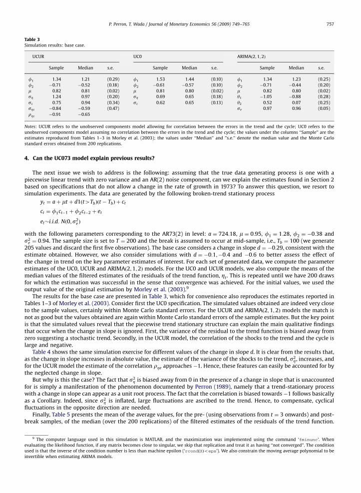
Table 3Simulation results: base case.

UCUR UC0 ARIMAð2;1;2Þ

Sample Median s.e. Sample Median s.e. Sample Median s.e.

f1 1.34 1.21 (0.29) f1 1.53 1.44 (0.10) f1 1.34 1.23 (0.25)

f2 �0.71 �0.52 (0.18) f2 �0.61 �0.57 (0.10) f2 �0.71 �0.44 (0.20)

m 0.82 0.81 (0.02) m 0.81 0.80 (0.02) m 0.82 0.80 (0.02)

sZ 1.24 0.97 (0.20) sZ 0.69 0.65 (0.18) y1 �1.05 �0.88 (0.28)

se 0.75 0.94 (0.34) se 0.62 0.65 (0.13) y2 0.52 0.07 (0.25)

sZe �0.84 �0.59 (0.47) se 0.97 0.96 (0.05)

rZe �0.91 �0.65

Notes: UCUR refers to the unobserved components model allowing for correlation between the errors in the trend and the cycle; UC0 refers to the

unobserved components model assuming no correlation between the errors in the trend and the cycle; the values under the columns ‘‘Sample’’ are the

estimates reproduced from Tables 1–3 in Morley et al. (2003); the values under ‘‘Median’’ and ’’s.e.’’ denote the median value and the Monte Carlo

standard errors obtained from 200 replications.


4. Can the UC073 model explain previous results?

The next issue we wish to address is the following: assuming that the true data generating process is one with apiecewise linear trend with zero variance and an AR(2) noise component, can we explain the estimates found in Section 2based on specifications that do not allow a change in the rate of growth in 1973? To answer this question, we resort tosimulation experiments. The data are generated by the following broken-trend stationary process

yt ¼ aþ mt þ d1ðt4TbÞðt � TbÞ þ ct

ct ¼ f1ct�1 þf2ct�2 þ et

et�i:i:d: Nð0;s2e Þ

with the following parameters corresponding to the AR73(2) in level: a ¼ 724:18, m ¼ 0:95, f1 ¼ 1:28, f2 ¼ �0:38 ands2

e ¼ 0:94. The sample size is set to T ¼ 200 and the break is assumed to occur at mid-sample, i.e., Tb ¼ 100 (we generate205 values and discard the first five observations). The base case considers a change in slope d ¼ �0:29, consistent with theestimate obtained. However, we also consider simulations with d ¼ �0:1;�0:4 and �0:6 to better assess the effect ofthe change in trend on the key parameter estimates of interest. For each set of generated data, we compute the parameterestimates of the UC0, UCUR and ARIMAð2;1;2Þ models. For the UC0 and UCUR models, we also compute the means of themedian values of the filtered estimates of the residuals of the trend function, Zt . This is repeated until we have 200 drawsfor which the estimation was successful in the sense that convergence was achieved. For the initial values, we used theoutput value of the original estimation by Morley et al. (2003).9

The results for the base case are presented in Table 3, which for convenience also reproduces the estimates reported inTables 1–3 of Morley et al. (2003). Consider first the UC0 specification. The simulated values obtained are indeed very closeto the sample values, certainly within Monte Carlo standard errors. For the UCUR and ARIMAð2;1;2Þ models the match isnot as good but the values obtained are again within Monte Carlo standard errors of the sample estimates. But the key pointis that the simulated values reveal that the piecewise trend stationary structure can explain the main qualitative findingsthat occur when the change in slope is ignored. First, the variance of the residual to the trend function is biased away fromzero suggesting a stochastic trend. Secondly, in the UCUR model, the correlation of the shocks to the trend and the cycle islarge and negative.

Table 4 shows the same simulation exercise for different values of the change in slope d. It is clear from the results that,as the change in slope increases in absolute value, the estimate of the variance of the shocks to the trend, s2

Z, increases, andfor the UCUR model the estimate of the correlation rZe approaches �1. Hence, these features can easily be accounted for bythe neglected change in slope.

But why is this the case? The fact that s2Z is biased away from 0 in the presence of a change in slope that is unaccounted

for is simply a manifestation of the phenomenon documented by Perron (1989), namely that a trend-stationary processwith a change in slope can appear as a unit root process. The fact that the correlation is biased towards �1 follows basicallyas a Corollary. Indeed, since s2

Z is inflated, large fluctuations are ascribed to the trend. Hence, to compensate, cyclicalfluctuations in the opposite direction are needed.

Finally, Table 5 presents the mean of the average values, for the pre- (using observations from t ¼ 3 onwards) and post-break samples, of the median (over the 200 replications) of the filtered estimates of the residuals of the trend function.

9 The computer language used in this simulation is MATLAB, and the maximization was implemented using the command ‘fminunc’. When

evaluating the likelihood function, if any matrix becomes close to singular, we skip that replication and treat it as having ‘‘not converged’’. The condition

used is that the inverse of the condition number is less than machine epsilon (‘rcondðXÞoeps’). We also constrain the moving average polynomial to be

invertible when estimating ARIMA models.

ARTICLE IN PRESS

Table 4Simulation results: effect of varying the change in slope d.

d ¼ �0:1 d ¼ �0:4 d ¼ �0:6

Median s.e. Median s.e. Median s.e.

(a) UCUR

f1 1.24 (0.26) 1.12 (0.28) 0.99 (0.29)

f2 �0.51 (0.16) �0.48 (0.16) �0.40 (0.18)

m 0.90 (0.02) 0.75 (0.02) 0.65 (0.02)

sZ 0.74 (0.37) 1.15 (0.16) 1.39 (0.15)

se 0.83 (0.28) 1.08 (0.33) 1.27 (0.38)

sZe �0.28 (0.43) �0.95 (0.50) �1.52 (0.65)

rZe �0.46 �0.76 �0.86

(b) UC0

f1 1.32 (0.10) 1.47 (0.11) 1.51 (0.11)

f2 �0.45 (0.11) �0.62 (0.11) �0.67 (0.13)

m 0.90 (0.01) 0.75 (0.02) 0.65 (0.02)

sZ 0.31 (0.26) 0.75 (0.16) 0.84 (0.25)

se 0.86 (0.13) 0.55 (0.15) 0.48 (0.21)

(c) ARIMAð2;1;2Þ

f1 1.26 (0.27) 1.15 (0.36) 1.03 (0.47)

f2 �0.45 (0.20) �0.45 (0.23) �0.33 (0.25)

m 0.90 (0.01) 0.75 (0.02) 0.65 (0.19)

y1 �1.00 (0.29) �0.80 (0.38) �0.64 (0.49)

y2 0.09 (0.25) 0.13 (0.26) 0.12 (0.28)

se 0.95 (0.05) 0.97 (0.05) 0.99 (0.05)


unobserved components model assuming no correlation between the errors in the trend and the cycle; the values under ‘‘Median’’ and ‘‘s.e.’’ denote the

median value and the Monte Carlo standard errors obtained from 200 replications.

Table 5Simulation results: filtered estimates of the residuals of the trend function Ztjt .

Sample mean Simulated

UCUR UC0 UCUR UC0

(a) Sample mean and simulated values with d ¼ �0:29

Full sample �0.003 0.004 0.003 0.012

Pre-break 0.159 0.148 0.144 0.136

Post-break �0.168 �0.142 �0.139 �0.109

d �0.1 �0.4 �0.6

UCUR UC0 UCUR UC0 UCUR UC0

(b) Simulated values for different values of d

Full sample 0.008 0.011 �0.002 0.004 �0.004 0.008

Pre-break 0.048 0.030 0.208 0.189 0.294 0.278

Post-break �0.030 �0.009 �0.205 �0.176 �0.293 �0.254


unobserved components model assuming no correlation between the errors in the trend and the cycle; d is the size of the change in the slope of the trend

function; the pre- and post-break samples are separated in 1973:1 for the sample values and at observation 100 out of a total sample size of 200 in the

simulations.


The results confirm the following features: (1) for both the UC0 and UCUR models, the mean is positive for the pre-breakperiod and negative for the post-break period; (2) the difference is bigger for the UCUR model than for the UC0 model(recall that the cyclical component also shows a change in level for the UC0 model); (3) the spread increases as themagnitude of the change increases; (4) the base case with d ¼ �0:29 delivers values quite close to the sample estimates. Insummary, our model is encompassing since it not only provides a better description of the data but also explains the resultsobtained from standard models that do not allow for a change in slope.

ARTICLE IN PRESS


5. Additional evidence without the need to specify a break date

In the previous sections, our analysis was conditional on the imposition of a fixed break date, 1973:1. In practice, onewould like a method that does not pre-supposes a choice for such a break date but delivers it as an outcome of thetrend–cycle decomposition procedure. Our aim in this section is to consider a class of unobserved components models thatis able to capture structural changes in the trend function endogenously. This type of model is not new and has been usedin the statistics literature to model structural changes; see, in particular, Kitagawa (1987), Gerlach et al. (2000), Giordaniet al. (2007) and for an application to the nature of shocks to inflation, Bidarkota (2003), among others. However, to ourknowledge it has not been used to provide a flexible trend–cycle decomposition.

It is a generalized State Space model where some of the errors are non-normal. We shall extend it to allow us to addressthe problems of interest and show how it can be a powerful tool for issues related to trend–cycle decompositions and,hence, a viable avenue for further developments.10 The specification used here is not the most general but is well suited tothe problems addressed. To understand the need for the key ingredients, let us go back to the generalized trend function


bt ¼ bt�1 þ vt ð4Þ

As stated in Remark 1, this specification provides very similar results compared to the case where bt is assumed fixed, whenthe noise to the slope component bt is assumed i:i:d: Nð0;s2

vÞ. The reason is that any positive variance s2v would imply

changes in the slope occurring at every period, though of different magnitudes each time, and the real GDP series wouldthen be Ið2Þ, a feature not supported by the data. Now, if our proposed specification is adequate, the slope of the trendfunction changes very rarely, indeed it is expected to change only once, or if the change occurs smoothly, for a few periodsaround 1973:1. This is the key observation and it suggests the use of a non-normal distribution for the errors vt . The naturalone to adopt in our context is a mixture of normal distributions where a realization of vt is a draw from one of two normaldistributions, one with high and the other with small or zero variance. More specifically,

vt ¼ ltg1t þ ð1� ltÞg2t ð5Þ

where git�i:i:d: Nð0;s2giÞ and lt is a Bernoulli random variable that takes value one with probability a1, and value 0 with

probability 1� a1. In our case, we would expect a1 to be close to one and s2g1 to be zero, so that most of the time there is no

change in the slope of the trend function. Furthermore, if s2g240, there will be occasional changes to the value of the slope.

Hence, this specification appears ideally suited to the problems we face. It is important to note that the probabilities thatthe errors be drawn from one regime or the other are independent of past realizations. This is in contrast to the popularMarkov switching type model (e.g., Hamilton, 1989). Here the different regimes affect the magnitude of the shocks and notper se what regime is in effect. Our goal is to have a framework which can allow special events such as a one-timeproductivity slowdown. Hence, the probability that we draw from the high variance distribution should be independent ofwhether past draws came from the small or large variance distributions. Accordingly, it is more appropriate to make theprobabilities of being in one regime or the other as independent of past realizations. Note also that using a mixture ofnormal distributions is better suited than using a t-distribution as in, say, Durbin and Koopman (2001). The latter indeedallows accounting for outliers but it remains that at each period there is a shock occurring. Since we wish to allow extendedperiods of time with no shock this approach is not useful.

More generally, the unobserved component model we propose is the following:

yt ¼ tt þ ct þot ð6Þ

where tt is specified by (4) with Zt�i:i:d: Nð0;s2ZÞ and vt is generated by the mixture distribution (5). The component ot is

introduced to capture measurement errors and is assumed to be i:i:d: Nð0;s2oÞ. The cyclical component will still be assumed

to be an AR(2)11 but we shall also generalize it to have shocks generated by a mixture of normals as well, i.e., we have

ct ¼ f1ct�1 þf2ct�2 þ et ð7Þ

where

et ¼ dtx1t þ ð1� dtÞx2t ð8Þ

with xit�i:i:d: Nð0;s2xiÞ and dt a Bernoulli random variable that takes value one with probability a2, and value 0 with

probability 1� a2. This generalization is made to potentially capture the fact that the variance of recessions may bedifferent from the variance of expansions. So the complete model consists of the specifications (4)–(8) with the addedassumption that all error terms and Bernoulli random variables are mutually independent. Note that we do not impose a

10 Additional evidence about the usefulness of the methodology proposed in this section is presented in Wada (2006) and Wada and Perron (2006)

who generalize the method and apply it to a wide variety of series.11 We use the AR(2) structure to keep close to the model analyzed in the previous sections and clearly see the implications of the changes introduced.

But more importantly, it provides a good approximation. Alternative specifications would be possible, see, e.g., Harvey and Trimbur (2003).

ARTICLE IN PRESS

Table 6Parameter estimates of the Gaussian mixture model.

Estimate s.e.

sZ 0.0004 0.2861

sx1 0.2583 0.1388

sx2 1.2816 0.1643

sg1 0.0001 0.0925

sg2 0.0634 0.3405

so 0.2497 0.0421

f1 1.3800 0.0640

f2 �0.4719 0.0609

a1 0.9000 1.0763

a2 0.5813 0.0986

lnðLÞ ¼ �271:3898

Notes: lnðLÞ is the value of the likelihood function evaluated at the maximum likelihood estimates; s.e. stands for the standard errors of the estimates.


change in the variance of the shock to reflect the so-called great-moderation (e.g., Stock and Watson, 2002). The goal is tohave a flexible trend–cycle decomposition that allows one to deduce such a feature.

The State Space model is of the form

yt ¼ Hxt þot

xt ¼ Fxt�1 þ Gut

where xt ¼ ½tt ; ct ; ct�1;bt�0, H ¼ ½1;1;0;0�

F ¼

1 0 0 1

0 f1 f2 0

0 1 0 0

0 0 0 1

26664

37775; G ¼

1 0 0

0 1 0

0 0 0

0 0 1

26664

37775

and ut ¼ ½Zt ; et ;vt�0. What is different from the usual State Space model is that the distribution of ut is not normal. However,

we can view the specification as a State Space model with normal errors but with four possible states. These states aredefined by the combined values of the Bernoulli random variables lt and dt and imply four possible covariance matrices forthe vector of errors ut , namely

Q ¼

s2Z 0 0

0 s2g1 0

0 0 s2x1

26664

37775;

s2Z 0 0

0 s2g1 0

0 0 s2x2

26664

37775;

s2Z 0 0

0 s2g2 0

0 0 s2x1

26664

37775;

s2Z 0 0

0 s2g2 0

0 0 s2x2

26664

37775

8>>><>>>:

9>>>=>>>;

where each component occurs with probabilities a1a2, a1ð1� a2Þ, ð1� a1Þa2, and ð1� a1Þð1� a2Þ, respectively. Thisinterpretation is helpful in constructing an algorithm for estimation.

Our generalization complicates the estimation procedure considerably and details are given in Appendix C. The basicprinciples are, however, the same as for the estimation of the usual State Space model with normal errors. The likelihoodfunction is estimated using a variant of the Kalman filter and a by-product is an estimate of the conditional expectation ofthe state vector xt using information available up to time t. These are denoted xtjt and are called filtered estimates. One canalso construct estimates using the full sample, i.e., xtjT which are obtained using a smoothing algorithm and are,accordingly, called smoothed estimates. The main goal here is to obtain smoothed estimates of the trend function tt and ofthe cyclical component ct .

It is important to note that, using Lemma 1 of Gerlach et al. (2000), the parameters a1, s2g1 and s2

g2 are not identified,though the trend–cycle decomposition is. To get parameter estimates we impose the following restrictions: a140:9,s2g1o0:0001, s2

g1os2g2 and s2

x1os2x2. The last two restrictions are standard and inconsequential. The first two are, however,

more substantive. They impose the variance of the state occurring with highest probability to be very small and the latterprobability to be quite high. This is to allow for the possibility of having relatively rare events occurring to the trendfunction. We tried many variations on the constraints and in no case was there a change in the trend–cycle decompositionand in the estimates of the other parameters of the model.

5.1. Discussion of the results

The results are presented in Table 6 and Fig. 3. The most important element is the smoothed trend–cycle decompositionpresented in the bottom panel of Fig. 3. It shows a trend and a cycle that are qualitatively similar to those obtained

ARTICLE IN PRESS

1950 1960 1970 1980 1990720

740

760

780

800

820

840

860

880

900

year

Trend

Data

1950 1955 1960 1965 1970 1975 1980 1985 1990 1995-10

-8

-6

-4

-2

0

2

4

6

8

10

year

1950 1960 1970 1980 1990720

740

760

780

800

820

840

860

880

900

year

Trend

Data

1950 1955 1960 1965 1970 1975 1980 1985 1990 1995-10

-8

-6

-4

-2

0

2

4

6

8

10

year

Dev

iatio

n (%

)D

evia

tion

(%)

Fig. 3. Trend and cycle decompositions of the Gaussian mixture model (the shaded areas are the periods of recessions as defined by the NBER). (Top left)

Data and filtered trend, (top right) filtered cycle, (bottom left) smoothed trend, (bottom right) smoothed cycle.


imposing an exogenous break in the slope of the trend in 1973:1. To better understand its properties, it is useful to look atthe parameters estimates presented in Table 6.

First, and most important, is the fact that the estimate of the variance of the residuals of the trend function s2Z is

nearly 0. Hence, except for changes in the slope bt , the trend is deterministic. The innovations to the trend function aregoverned by a process that has standard deviation 0.0001 with probability 0.9 and one that has standard deviation 0.0633with probability 0.10. These estimates are, however, highly dependent on the restrictions imposed and we shall returnbelow with a better method to identify the pattern of the slope of the trend function. But the basic message is clear, most ofthe time the slope does not vary. A look at Fig. 3 suggests that the changes occur smoothly around 1973:1.

Other estimates are also very informative. The noise of the cyclical component also consists of draws from normaldistributions with very different variances. With probability 0.58 the standard deviation is small at the value 0.26, and withprobability 0.42 it is high at the value 1.28. We interpret these results as follows. The variance of shocks in recessions ismuch larger than the variance of shocks in expansions. A look at the smoothed cycle in Fig. 3 shows this to be indeed thecase. Recessions are much more pronounced than expansions. This accords well with previous studies on business cyclesasymmetries; see, e.g., Beaudry and Koop (1993), Neftci (1984) and Sichel (1993, 1994). The reduction in volatility after1985 is also apparent from the plotted cycle. The parameter estimates of the AR coefficients are well within the stationaryregion, the sum being close to 0.91. The variance of the measurement errors is quite small and does not account for much ofthe movements of real GDP. Finally, note that the value of the maximized likelihood function is �271:4, well above that forthe models discussed earlier.

ARTICLE IN PRESS

1950 1960 1970 1980 19900.4

0.5

0.6

0.7

0.8

0.9

1

1.1

year

slop

e

Fig. 4. Smoothed estimates of the slope of the trend function. (The dashed lines correspond to 1, 2 and 3 standard deviations confidence intervals.)

Table 7Estimates for the Gaussian mixture model of the filtered trend.

Estimate s.e.

sZ 0.4655 0.0233

sg1 0.0001 0.1250

sg2 1.0757 1.2591

a 0.9992 0.0009

lnðLÞ ¼ �137:5639

Notes: lnðLÞ is the value of the likelihood function evaluated at the maximum likelihood estimates; s.e. stands for the standard errors of the estimates.


The smoothed estimate of the cycle shares many of the interesting features that were present for the models with anexogenous change in 1973:1. First, the movements agree quite well with the NBER chronology. Second, the late 1990s are,as should be expected, characterized by above trend activity. Third, as alluded to above, recessions are characterized bysharp drops in activity, while expansions are gradual increases. Fourth, the sharpest recession is that of 1982, while ourmodel with an exogenous change in slope and symmetric errors for the cyclical component indicated the recession of 1958as the sharpest. Fifth, depth of recessions are larger than highs of expansions in the sense that recessions are oftencharacterized by a value 6–8 percentage points below trend, while expansions are characterized by values that reachbetween 2 and 4 percentage points above trend.

The filtered estimates of the trend and cycles also show some interesting features. This filtered decomposition gives thebest estimates of the trend and cycle using only information available up to the current period. One fact is that the slope ofthe trend seemed to be on the increase in the late 1990s. This accords well with discussions at the time that the trend mayhave been on a new path with the new information technology. However, a comparison with the smoothed trend, whichuses all information in the sample, shows this hope not to have materialized (at least by the end of 1998). Another featureof interest is that the sharpness of the 1991 recession was ex post more severe than what could have been inferred at thetime.

We believe these results to be in accordance with common notions about the business cycles and to lend credence toour framework as a general methodology for trend–cycle decomposition.

5.2. Filtered estimates for the slope of the trend function

As discussed, while the trend–cycle decomposition is well identified, the identification of some components is not. Sincethe temporal behavior of the slope of the trend function is of central concern here, we present a two-step method todocument it. We start with the filtered estimates of the trend function, ftt ¼ ttjtg, as the basic inputs (using the smoothedestimates leads to the same results). We then estimate the following model:


bt ¼ bt�1 þ vt ð9Þ

ARTICLE IN PRESS


where

Zt ¼ ðtt�1 � tt�1jt�1Þ � ðtt � ttjtÞ þ Zt

and vt is specified by the mixture of normal distributions (5). This model is simple enough that an exact numericalprocedure to obtain smoothed estimates of the slope is possible, i.e., btjT . The Fortran algorithm was constructed byKitagawa (1993) and we translated it in MATLAB for the estimation reported (see Appendix D for details). Note that eventhough the variance of Zt is zero, the variance of Zt is not since it depends of the filtered estimates ttjt whose variance isnon-null.

The results are presented in Fig. 4 and Table 7. The solid line is the smoothed estimate of the slope btjT and the dashedlines are 1, 2 and 3 standard deviations intervals. The results are quite informative and in line with our main argument. Theslope starts at a value 0.94 at the beginning of the sample and remains at that value until roughly the late 1960s when aminor decrease starts to take effect. The main change occurs in the period 1973–1974 when the slope decreases to a valueof approximately 0.75. Until 1977 there is a further gradual decline to a new value of 0.66 that remains in effect until theend of the sample.

1950 1955 1960 1965 1970 1975 1980 1985 1990 1995−10

0

10HP filter 1600

year

Dev

iatio

n (%

)

1950 1955 1960 1965 1970 1975 1980 1985 1990 1995−10

0

10Band Pass Filter

year

Dev

iatio

n (%

)

1950 1955 1960 1965 1970 1975 1980 1985 1990 1995−10

0

10

HP Filter 800,000

year

Dev

iatio

n (%

)

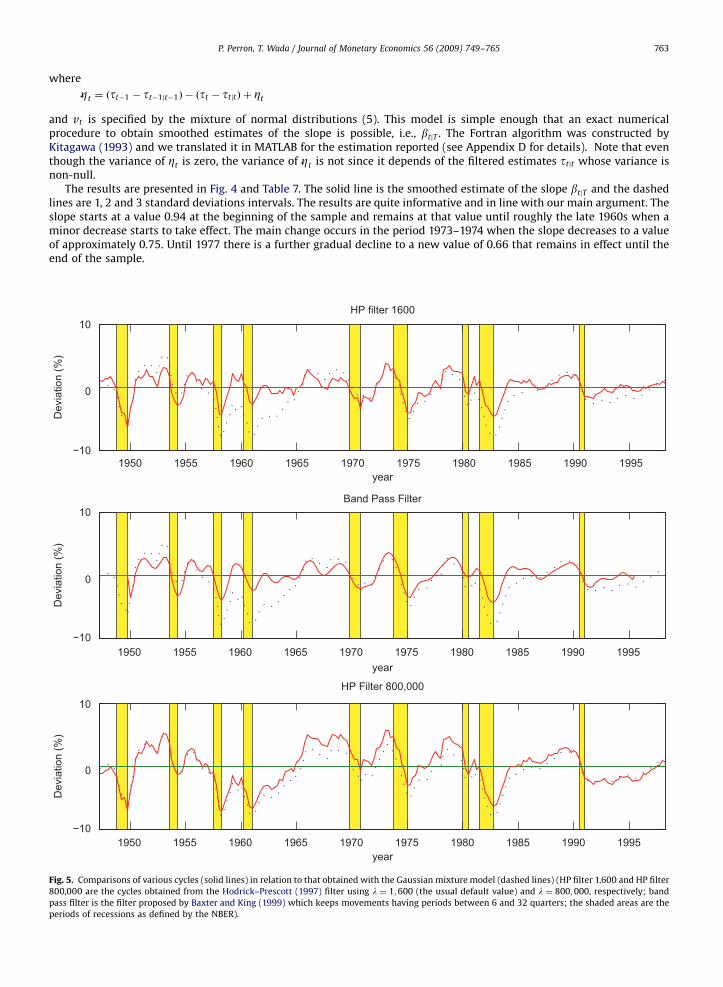
Fig. 5. Comparisons of various cycles (solid lines) in relation to that obtained with the Gaussian mixture model (dashed lines) (HP filter 1,600 and HP filter

800,000 are the cycles obtained from the Hodrick–Prescott (1997) filter using l ¼ 1;600 (the usual default value) and l ¼ 800;000, respectively; band

pass filter is the filter proposed by Baxter and King (1999) which keeps movements having periods between 6 and 32 quarters; the shaded areas are the

periods of recessions as defined by the NBER).

ARTICLE IN PRESS


These results lend support to the central theme of our work, namely that an important change in the slope of the trendfunction has occurred around the year 1973. While, the change depicted here is more gradual than the assumed suddenchange used in the previous sections, the message is the same. The change is important and is responsible for the severebiases arising when estimating models that neglect its presence. Finally, note that we repeated the estimation with anextended data set that goes up to 2004:2, with no change in the qualitative results.

6. Comparisons with other decompositions

Many trend–cycle decompositions have been suggested in the literature. Besides the Beveridge–Nelson decompositionand the unobserved components models examined previously, two other popular methods are the Hodrick–Prescott filterand the band-pass filter (Baxter and King, 1999). The former is a method to extract a trend function and delivers, as aconsequence, a cycle as the difference with the original series. The BP filter, however, does not address the issue of trendestimation directly. The cycle is defined as movements having periods between 6 and 32 quarters. Hence, both high andlow frequency movements are eliminated and the difference between the cycle obtained and the original series cannot beviewed as an estimate of the trend function.

In this section, we compare these trend and cycle extraction procedures with our decomposition. The first panel in Fig. 5presents the cycle obtained from the HP filter with the usual value of the smoothing parameter l ¼ 1;600. The secondpanel in Fig. 5 presents the cycle obtained using the two-sided BP filter suggested by Baxter and King (1999) with 12 termson each sides (accordingly the cycle is undefined for the first and last 12 quarters of the sample).

The cycles obtained are somewhat ‘‘in between’’ our decomposition and the BN cycle advocated by Morley et al. (2003).Both show much less variations than our cycle and slightly more than the BN cycle. Also, the movements are more frequentthan in our cycle but less so than in the BN cycle. Overall, they capture rather well the timing of the recessions (as does ourcycle) but the depth of the recessions and the heights of the expansions are very different. For example, both the HP and BPcycles show the sixties as a period of average activities or very mild expansion following a mild recession in 1961, whileours characterize the sixties as a period of important and sustained expansion following a deep recession in 1961. Otherdifferences can be ascertained from the graphs, but the most striking feature is the magnitude of the cycle. The HP trendbeing stochastic, a lot of the movements in real GDP are due to movements in the trend and little is left for the cycle. Whilethe BP filter does not estimate a trend directly, the overall picture is much the same. It should be stressed, however, that thecycle obtained with our decomposition offers the most contrasting picture of the cycle when compared to that obtainedwith the Beveridge–Nelson decomposition.

Finally, the last panel in Fig. 5 presents an interesting result about the HP filter. It gives the trend–cycle decompositionwhen the smoothing parameter is set to the very large number l ¼ 800;000. The results are then basically equivalent to ourdecomposition with a trend that has a single shift in slope in 1973. So we can, in a sense, reconcile our results with thedecomposition of the HP filter. The latter depends crucially on the choice of the smoothing parameter l and, as is wellknown, the best value depends on the underlying true structure of the process and the usual rule of thumb of settingl ¼ 1;600 is unlikely to be appropriate in most cases. Our decomposition does not suffer from such arbitrariness andsuggests that for the particular case of the real GDP series analyzed, l ¼ 1;600 is too small a value that has an effect ofascribing too much variation to the trend and too little to the cycle.

7. Concluding remarks

The central ingredient of our analysis is that once allowance is made for the possibility of a change in the slope of thetrend function for postwar US real GDP, results pertaining to trend–cycle decompositions are very different from thoseobtained using currently popular methods (Beveridge–Nelson or unobserved components decompositions, Hodrick–Prescott or band-pass filters). It also agrees much better with the NBER chronology and has the advantage of being able toexplain results pertaining to decompositions obtained by methods such as that of Beveridge–Nelson and the unobservedcomponents models. In particular, once a change in the slope of the trend function is permitted, these methods yield thesame decomposition with a non-stochastic trend (except for the change in 1973) and the negative correlation between theshock to the trend and to the cycle is no longer an issue.

We also presented a generalized unobserved components model based on errors that follow a mixture of normaldistributions. It was found to be successful in reaching the same conclusions without the need to make any priorspecifications about the nature or timing of the change in the slope. Such a framework should find wide appeal fortrend–cycle decompositions in a variety of contexts, when the trend path of some series is affected by infrequent levelshifts or changes in slope, when the noise function shows different variability across two regimes, or when the overallseries is affected by aberrant observations.

A useful generalization would be to allow for the possibility of correlation across the stochastic components of the trendand the cycle. While we have documented that such a feature is not present with the particular US real GDP series used,this may not be the case in general. Finally, while most decompositions used in applied work are based on univariatemethods, extensions to decompositions based on modeling multiple series jointly are important. More in-depthcomparisons of the implied cycles with other methods would also be useful.

ARTICLE IN PRESS


Appendix. Supplementary data

Supplementary data associated with this article can be found in the online version at doi:10.1016/j.jmoneco.2009.08.001.

References

Baxter, M., King, R.G., 1999. Measuring business cycles: approximate band-pass filters for economic time series. Review of Economics and Statistics 81,575–593.

Beaudry, P., Koop, G., 1993. Do recessions permanently change output?. Journal of Monetary Economics 31, 149–163.Beveridge, S., Nelson, C.R., 1981. A new approach to decomposition of economic time series into permanent and transitory components with particular

attention to measurement of the ‘business cycle’. Journal of Monetary Economics 7, 151–174.Bidarkota, P.V., 2003. Do fluctuations in U.S. inflation rates reflect infrequent large shocks or frequent small shocks?. Review of Economics and Statistics

85, 765–771.Burns, A.M., Mitchell, W.C., 1946. Measuring Business Cycles. National Bureau of Economic Research, New York.Campbell, J.Y., Mankiw, N.G., 1987. Are output fluctuations transitory?. Quarterly Journal of Economics 102, 857–880.Canova, F., 1998. Detrending and business cycle facts. Journal of Monetary Economics 41, 475–512.Canova, F., 1999. Does detrending matter for the determination of the reference cycle and the selection of turning points?. Economic Journal 109, 126–150.Cheung, Y.N., Chinn, M., 1997. Further investigation of the uncertain unit root in U.S. GDP. Journal of Business and Economic Statistics 15, 68–73.Christiano, L.J., 1992. Searching for breaks in GNP. Journal of Business and Economic Statistics 10, 237–250.Clark, P.K., 1987. The cycle component of the U.S. economic activity. Quarterly Journal of Economics 102, 797–814.Cochrane, J., 1988. How big is the random walk in GNP?. Journal of Political Economy 96, 893–920.Cogley, T., Nason, J.M., 1995. Output dynamics in real-business-cycle models. American Economic Review 85, 492–511.Durbin, J., Koopman, S.J., 2001. Time Series Analysis by State Space Methods. Oxford University Press, New York.Gali, J., 1999. Technology, employment, and the business cycle: Do technology shocks explain aggregate fluctuations?. American Economic Review 89,

249–271.Gerlach, R., Carter, C., Kohn, R., 2000. Efficient Bayesian inference for dynamic mixture models. Journal of the American Statistical Association 95, 819–828.Giordani, P., Kohn, R., van Dijk, D., 2007. A unified approach to nonlinearity, structural change, and outliers. Journal of Econometrics 137, 112–133.Hamilton, J.D., 1989. A new approach to the economic analysis of nonstationary time series and business cycles. Econometrica 57, 357–384.Hansen, G.D., 1997. Technical progress and aggregate fluctuations. Journal of Economic Dynamic and Control 21, 1005–1023.Harvey, A.C., Trimbur, T.M., 2003. General model-based filters for extracting cycles and trends in economic time series. Review of Economics and Statistics

85, 244–255.Hodrick, R., Prescott, E., 1997. Postwar US business cycles: an empirical investigation. Journal of Money, Credit, and Banking 29, 1–16.King, R.G., Plosser, C.I., Stock, J.H., Watson, M.W., 1991. Stochastic trend and economic fluctuations. American Economic Review 81, 819–840.Kitagawa, G., 1987. Non-Gaussian state-space modeling of nonstationary time series. Journal of American Statistic Association 82, 1032–1063.Kitagawa, G., 1993. FORTRAN77 Time Series Analysis Programming. Iwanami-Shoten, Tokyo (in Japanese).Morley, J.C., Nelson, C.R., Zivot, E., 2003. Why are Beveridge–Nelson and unobserved-component decompositions of GDP so different?. Review of

Economics and Statistics 85, 235–243.Neftci, S.N., 1984. Are economic time series asymmetric over the business cycles?. Journal of Political Economy 92, 307–328.Oh, K.H., Zivot, E., 2006. The Clark model with correlated components. Unpublished manuscript, Department of Economics, University of Washington.Perron, P., 1989. The great crash, the oil price shock and the unit root hypothesis. Econometrica 57, 1361–1401.Sichel, D.E., 1993. Business cycle asymmetry: a deeper look. Economic Inquiry, 224–236.Sichel, D.E., 1994. Inventories and the three phases of the business cycle. Journal of Business and Economic Statistics 12, 269–277.Stock, J.H., Watson, M.W., 1988. Variable trends in economic time series. Journal of Economic Perspectives 2, 147–174.Stock, J.H., Watson, M.W., 1998. Median unbiased estimation of coefficient variance in time-varying parameter model. Journal of American Statistical

Association 93, 349–358.Stock, J.H., Watson, M.W., 1999. Business cycle fluctuations in US macroeconomic time series. In: Taylor, J.B., Woodford, M. (Eds.), Handbook of

Macroeconomics, vol. 1A. North-Holland, Amsterdam.Stock, J.H., Watson, M.W., 2002. Has the business cycle changed and why?. In: Gertler, M., Rogoff, K. (Eds.), NBER Macroeconomics Annual, vol. 17. MIT

Press, Cambridge, MA, pp. 159–218.Wada, T., 2006. Trend–cycle decompositions allowing structural changes and outliers: econometric analyses with macroeconomic applications. Ph.D.

Dissertation, Department of Economics, Boston University.Wada, T., Perron, P., 2006. An alternative trend–cycle decomposition using a state space model with mixtures of normals: specifications and applications

to international data. Unpublished manuscript, Department of Economics, Boston University.Watson, M.W., 1986. Univariate detrending methods with stochastic trend. Journal of Monetary Economics 18, 49–75.Zarnowitz, V., Ozyildirim, A., 2007. Time series decompositions and measurement of business cycles, trends and growth cycles. Journal of Monetary

Economics 53, 1717–1739.Zivot, E., Andrews, D.W.K., 1992. Further evidence on the great crash, the oil-price shock and the unit root hypothesis. Journal of Business and Economic

Statistics 10, 251–287.

10.1016/j.jmoneco.2009.08.001

10.1016/j.jmoneco.2009.08.001

Documents

Let's take a break: Trends and cycles in US real GDP