Stellar Oscillations:Pulsations of Stars Throughout the H-R diagram

Mike Montgomery

Department of Astronomy and McDonald Observatory,The University of Texas at Austin

January 15, 2013

Stellar Oscillations

Why study stars inthe first place?

• Distance scales• Cepheids/RR Lyrae stars• Planetary Nebulae• Supernovae

• Ages• Main-Sequence turnoff• White Dwarf cooling

• Chemical Evolution• stellar nucleosynthesis• ISM enrichment

The Role of the Star in Astrophysics

The Role of the Star in Astrophysics

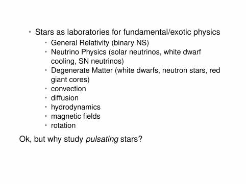
• Stars as laboratories for fundamental/exotic physics• General Relativity (binary NS)• Neutrino Physics (solar neutrinos, white dwarf

cooling, SN neutrinos)• Degenerate Matter (white dwarfs, neutron stars, red

giant cores)• convection• diffusion• hydrodynamics• magnetic fields• rotation

Ok, but why study pulsating stars?

Pulsations give us a differential view of a star:

• not limited to global quantities such asTeff and log g

• get a dynamic versus a static picture• can ‘see inside’ the stars, study stellar interiors

(‘helio- and asteroseismology’)• potential to measure rotation (solid body and

differential)• find thickness of convection zones

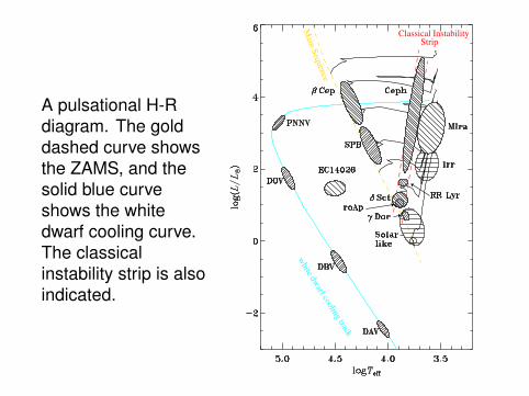
A pulsational H-Rdiagram. The golddashed curve showsthe ZAMS, and thesolid blue curveshows the whitedwarf cooling curve.The classicalinstability strip is alsoindicated.

white dw

arf cooling track

Classical InstabilityStrip

Main

Seq

uen

ce

Theory of Stellar Pulsations

• Stellar pulsations are global eigenmodesAssuming they have “small” amplitudes,they are …

• coherent fluid motions of the entire star• sinusoidal in time• the time-dependent quantities are characterized by

small departures about the equilibrium state of thestar

• the angular dependence is ∝ Y`m(θ, φ), if theequilibrium model is spherically symmetric

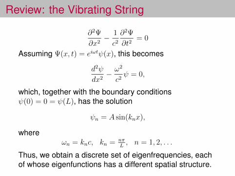
Review: the Vibrating String

∂2Ψ

∂x2− 1

c2

∂2Ψ

∂t2= 0

Assuming Ψ(x, t) = eiωtψ(x), this becomes

d2ψ

dx2− ω2

c2ψ = 0,

which, together with the boundary conditionsψ(0) = 0 = ψ(L), has the solution

ψn = A sin(knx),

whereωn = knc, kn = nπ

L, n = 1, 2, . . .

Thus, we obtain a discrete set of eigenfrequencies, eachof whose eigenfunctions has a different spatial structure.

Completely analogous to the case of pulsations of a star:(Montgomery, Metcalfe, & Winget 2003, MNRAS, 344, 657)

vibrating string stellar pulsations

wave equation ←→ fluid equations (e.g., massand momentum cons.)

frequencies (ωn) ←→ frequencies (ωn)

vertical displacement ←→radial displacement(δr), or pressure (δp)eigenfunction

1D spatial eigenfunction ←→ 1D in radius × 2Din θ, φ (Y`m(θ, φ))

The time dependence (eiωt) of both are identical

Stellar Hydrodynamics Equations• mass conservation

∂ρ

∂t+∇ · (ρv) = 0

• momentum conservation

ρ

(∂

∂t+ v · ∇

)v = −∇p− ρ∇Φ

• energy conservation

ρ T

(∂

∂t+ v · ∇

)S = ρ εN −∇ · F

• Poisson’s Equation∇2Φ = 4πGρ

Definitionsρ density T temperaturev velocity S entropyp pressure F radiative fluxΦ gravitational

potentialεN nuclear energy

generation rate

Stellar Hydrodynamics EquationsTo obtain the equations describing linear pulsations (Unno et al.1989, pp 87–104)

• perturb all quantities to first order (e.g.,p′, ρ′,v′ = v = ∂~ξ/∂t)

• assume p′(r, t) = p(r)Y`m(θ, φ) eiωt, and similarly for otherperturbed quantities

• rewrite in terms of, say, ξr and p′

Technical Aside:We use primes (e.g., p′) to refer to Eulerian perturbations(perturbations of quantities at a fixed point in space) and delta’s(δp) to refer to Lagrangian perturbations (evaluated in the frameof the moving fluid). The relationship between the two is

δp = p′ + ~ξ · ∇p,

where ~ξ is the displacement of the fluid.

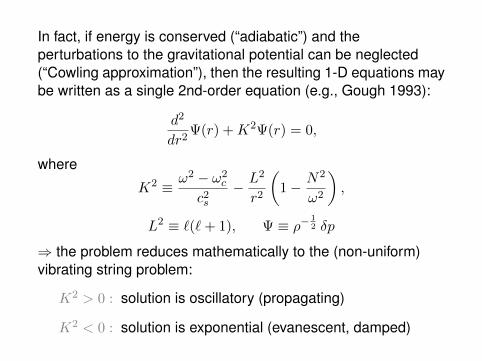
In fact, if energy is conserved (“adiabatic”) and theperturbations to the gravitational potential can be neglected(“Cowling approximation”), then the resulting 1-D equations maybe written as a single 2nd-order equation (e.g., Gough 1993):

d2

dr2Ψ(r) +K2Ψ(r) = 0,

where

K2 ≡ ω2 − ω2c

c2s

− L2

r2

(1− N2

ω2

),

L2 ≡ `(`+ 1), Ψ ≡ ρ−12 δp

⇒ the problem reduces mathematically to the (non-uniform)vibrating string problem:

K2 > 0 : solution is oscillatory (propagating)

K2 < 0 : solution is exponential (evanescent, damped)

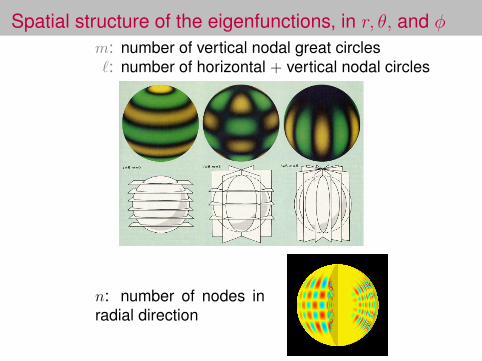
Spatial structure of the eigenfunctions, in r, θ, and φm: number of vertical nodal great circles`: number of horizontal + vertical nodal circles

n: number of nodes inradial direction

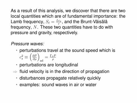
As a result of this analysis, we discover that there are twolocal quantities which are of fundamental importance: theLamb frequency, S` = Lcs

r, and the Brunt-Väisälä

frequency, N . These two quantities have to do withpressure and gravity, respectively.

Pressure waves:• perturbations travel at the sound speed which isc2s ≡

(∂P∂ρ

)ad

= Γ1Pρ

• perturbations are longitudinal⇒ fluid velocity is in the direction of propagation

• disturbances propagate relatively quickly• examples: sound waves in air or water

The Brunt-Väisälä frequency, N , is a local buoyancyfrequency, which owes its existence to gravity.

Gravity waves:• perturbations are transverse⇒ fluid velocity is perpendicular to the direction of

propagation of the wave• disturbances propagate relatively slowly• medium must be stratified (non-uniform)

Example: surface water waves

Amplitude particle motion

v =1

2(gλ)1/2

Can we calculate N physically?

Fluid element isdisplaced fromits equilibriumposition.

Assume• pressure equilibrium• no energy exchange (“adiabatic”)

P (r + δr) = P (r) +

(∂P

∂ρ

)ad

δρ

⇒ δρ =ρ

Γ1P

dP

drδr

• density difference, ∆ρ, with new surroundings:∆ρ = ρ(r) + δρ− ρ(r + δr)

=ρ

Γ1P

dP

drδr − dρ

drδr

• applying F = ma to this fluid element yields

ρd2δr

dt2= −g∆ρ

= −ρg(

1

Γ1

d lnP

dr− d ln ρ

dr

)δr

d2δr

dt2= − g

(1

Γ1

d lnP

dr− d ln ρ

dr

)︸ ︷︷ ︸

N2

δr

N2 > 0: fluid element oscillates about equilibrium positionwith frequency N

N2 < 0: motion is unstable⇒ convection (Schwarzschildcriterion)

Mode Classification

Depending upon whether pressure or gravity is the dominantrestoring force, a given mode is said to be locally propagatinglike a p-mode or a g-mode. This is determined by the frequencyof the mode, ω.

Ford2

dr2Ψ(r) +K2Ψ(r) = 0,

Gough (1993) showed that K2 could be written as

K2 =1

ω2c2(ω2 − ω2

+)(ω2 − ω2−),

whereω+ ≈ S` ≡

Lcsr, ω− ≈ N

Mode Classification

Whether a mode is locally propagating or evanescent isdetermined by its frequency relative to S` and N :

p-modes: ω2 > S2` , N

2 (“high-frequency”)K2 > 0, mode is locally “propagating”

g-modes: ω2 < S2` , N

2 (“low-frequency”)K2 > 0, mode is locally “propagating”

However, ifmin(N2, S2

` ) < ω2 < max(N2, S2` ),

thenK2 < 0,

and the mode is not locally propagating, and is termed‘evanescent’, ‘exponential’, or ‘tunneling’.

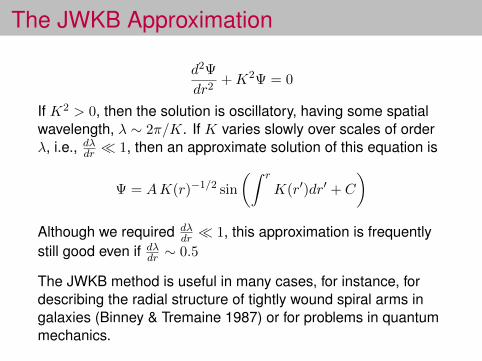
The JWKB Approximation

d2Ψ

dr2+K2Ψ = 0

If K2 > 0, then the solution is oscillatory, having some spatialwavelength, λ ∼ 2π/K. If K varies slowly over scales of orderλ, i.e., dλdr 1, then an approximate solution of this equation is

Ψ = AK(r)−1/2 sin

(∫ r

K(r′)dr′ + C

)Although we required dλ

dr 1, this approximation is frequentlystill good even if dλdr ∼ 0.5

The JWKB method is useful in many cases, for instance, fordescribing the radial structure of tightly wound spiral arms ingalaxies (Binney & Tremaine 1987) or for problems in quantummechanics.

Asymptotic Analysis: The JWKB Approximation

Satisfying the boundary conditions for a modepropagating between r1 and r2 yields the following“quantization” condition:∫ r2

r1

drK = nπ.

For high frequencies, K ∼ ω/c, so this leads to

ω =nπ∫dr c−1

⇒ frequencies are evenly spaced as a function of radialovertone number n (just like the vibrating string).

Asymptotic Analysis: The JWKB Approximation

For low frequencies, K ∼ LN/ωr, so this leads to

ω =L

nπ

∫dr N/r,

so

P =2nπ2

L

[∫dr N/r

]−1

.

⇒ periods are evenly spaced as a function of radialovertone number n.

Example: propagation diagram for a white dwarf model

p-modes

g-modes300 sec

center surface

Driving Pulsations: The Adiabatic Assumption

Adiabatic: No heat gain or loss during a pulsation cycle,i.e., dqdt = 0

One way to quantify this is to compare the energy content“stored” in the layers in the star above a certain point, ∆qs, withthe energy which passes through these layers in one pulsationperiod, ∆ql:

∆qs ∼ CV T ∆Mr

Here ∆Mr ≡M? −Mr is the envelope mass. The energypassing through this layer in one pulsation period, Π, is

∆ql ∼ Lr Π,

where Lr is the luminosity at radius r.

Driving Pulsations: The Adiabatic Assumption

In order for the adiabatic approximation to be valid we need∆ql ∆qs, which implies that

η ≡ Lr Π

CV T ∆Mr 1

In general, CV ∼ 109 ergs/g-K, and for solar p-modes,Π ∼ 300 sec. Using solar values for Lr and Mr we find

• η ∼ 10−16 in the inner regions of the sun

• η ∼ 1 at ∆Mr/M ∼ 10−10

In other words, η 1 throughout the vast majority of the Sun.

Driving Pulsations: Mechanisms

Without some mechanism to drive the pulsations, finiteamplitude eigenmodes would not be observed in starsTwo classes of driven modes:linearly unstable: Mode amplitudes grow exponentially in

time until quenched by nonlinear effects(“large amplitude pulsators”), e.g., modesradiatively driven by the “Kappa-gammamechanism”.

stochastically driven: Modes are intrinsically stable, butare dynamically excited (“hit”) by theconvective motions, and then decay away(“solar-like, low amplitude pulsators”), e.g.,driven by turbulent motions of the convectionzone.

Linear Driving/Amplification

• A mode which is linearly unstable will increase itsamplitude with time

• infinitesimal perturbations are linearly amplified(“self-amplified”), grow exponentially

• Example: the harmonic oscillator

x+ γ x+ ω20 x = 0

⇒ x(t) = Aeγ t/2 cosω t,

whereω =

√ω2

0 − γ2/4.

So amplitude grows in time as eγ t/2.

Linear Driving/Amplification

Several mechanisms exist which can do this:

nuclear driving: “the epsilon mechanism”radiative driving: “the kappa mechanism”

• In order to drive locally, energy must be flowing into aregion at maximum compression

• Typically, only a few regions of a star can drive amode, but the mode is radiatively dampedeverywhere else. For a mode to grow, the totaldriving has to exceed the total damping

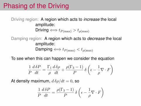
Phasing of the Driving

Driving region: A region which acts to increase the localamplitude:Driving⇐⇒ tP (max) > tρ(max)

Damping region: A region which acts to decrease the localamplitude:Damping⇐⇒ tP (max) < tρ(max)

To see when this can happen we consider the equation

1

P

d δP

dt=

Γ1

ρ

d δρ

dt+ρ(Γ3 − 1)

Pδ

(ε− 1

ρ∇ · F

)At density maximum, d δρ/dt = 0, so

1

P

d δP

dt=ρ(Γ3 − 1)

Pδ

(ε− 1

ρ∇ · F

)

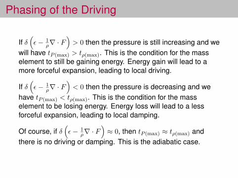
Phasing of the Driving

If δ(ε− 1

ρ∇ · F)> 0 then the pressure is still increasing and we

will have tP (max) > tρ(max). This is the condition for the masselement to still be gaining energy. Energy gain will lead to amore forceful expansion, leading to local driving.

If δ(ε− 1

ρ∇ · F)< 0 then the pressure is decreasing and we

have tP (max) < tρ(max). This is the condition for the masselement to be losing energy. Energy loss will lead to a lessforceful expansion, leading to local damping.

Of course, if δ(ε− 1

ρ∇ · F)≈ 0, then tP (max) ≈ tρ(max) and

there is no driving or damping. This is the adiabatic case.

The Kappa-gamma MechanismConsider a temperature perturbation δT/T which isindependent of position:

In equilibrium, F1 = F2. Now consider perturbations only to theopacity due to the temperature perturbation. Since

F = − 4ac

3κρT 3∇T ∝ 1/κ,

we have δF = −F δκ

κ= −Fδ lnκ = −F ∂ lnκ

∂ lnT

δT

T

The flux going in minus the flux leaving is

∆F ≡ F1 + δF1 − (F2 + δF2)

= −F δT

T

[(∂ lnκ

∂ lnT

)r1

−(∂ lnκ

∂ lnT

)r2

]= F

δT

Th

(d

drκT

),

whereκT ≡

(∂ lnκ

∂ lnT

)ρ

.

Thus, we have local driving if

d

drκT > 0

This condition is fulfilled in the outer partial ionization zones ofmany stars.

A more careful derivation(including densityperturbations in thequasi-adiabaticapproximation) shows thatthe condition for local drivingdue to the Kappa-gammamechanism is actually

d

dr[κT + κρ/(Γ3 − 1)] > 0,

where Γ3 − 1 ≡(∂ lnT∂ ln ρ

)S.

Timescales and DrivingA region which can locally drive modes (e.g., He II partialionization) most effectively drives modes whose periods areclose to the thermal timescale of the region:

τthermal ∼∆MrcV T

Ltot∼ P (mode period)

Timescales

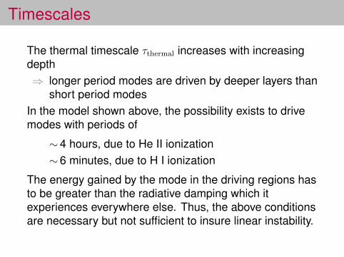
The thermal timescale τthermal increases with increasingdepth⇒ longer period modes are driven by deeper layers than

short period modesIn the model shown above, the possibility exists to drivemodes with periods of

∼4 hours, due to He II ionization∼6 minutes, due to H I ionization

The energy gained by the mode in the driving regions hasto be greater than the radiative damping which itexperiences everywhere else. Thus, the above conditionsare necessary but not sufficient to insure linear instability.

A More Detailed (but still qualitative)Calculation of κ-γ Driving

ρ Tds

dt= ρ ε−∇ · ~F

Again, let’s assume a perturbation with δT/T constant in space.For a region in the envelope, ε = 0, and let’s qualitatively writeT ds ≈ cV dT/T , so

ρ cVdT

dt= −∇ · ~F = −∂Fr

∂r

Ignoring differences between δ and ′, we consider the effect of aperturbation in δT :

ρ cVd δT

dt= −∂ δFr

∂r

Fr ∝ −∇T 4

κ⇒ δFr

Fr= −δκ

κ+ 4

δT

T

Calculation of κ-γ Driving

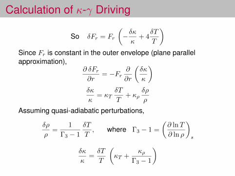
So δFr = Fr

(−δκκ

+ 4δT

T

)Since Fr is constant in the outer envelope (plane parallelapproximation),

∂ δFr∂r

= −Fr∂

∂r

(δκ

κ

)δκ

κ= κT

δT

T+ κρ

δρ

ρ

Assuming quasi-adiabatic perturbations,

δρ

ρ=

1

Γ3 − 1

δT

T, where Γ3 − 1 =

(∂ lnT

∂ ln ρ

)s

δκ

κ=δT

T

(κT +

κρΓ3 − 1

)

Calculation of κ-γ Driving

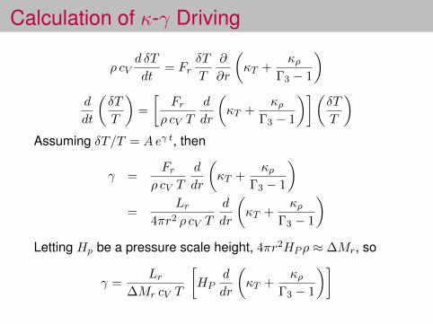
ρ cVd δT

dt= Fr

δT

T

∂

∂r

(κT +

κρΓ3 − 1

)d

dt

(δT

T

)=

[Fr

ρ cV T

d

dr

(κT +

κρΓ3 − 1

)](δT

T

)Assuming δT/T = Aeγ t, then

γ =Fr

ρ cV T

d

dr

(κT +

κρΓ3 − 1

)=

Lr4πr2 ρ cV T

d

dr

(κT +

κρΓ3 − 1

)Letting Hp be a pressure scale height, 4πr2HPρ ≈ ∆Mr, so

γ =Lr

∆Mr cV T

[HP

d

dr

(κT +

κρΓ3 − 1

)]

Calculation of κ-γ Driving

In terms of the thermal timescale this is

γ = τ−1th

[HP

d

dr

(κT +

κρΓ3 − 1

)]The term in brackets is O(1), although it can be as large as 10.Thus, the local growth rate can be as large as τ−1

th , and weagain see that

d

dr

(κT +

κρΓ3 − 1

)> 0

is the criterion for local driving to occur. In practice, this alwaysoccurs in a partial ionization (PI) zone of some element.

Of course, the total growth rate for a mode is summed over theentire star, which includes driving and damping regions, and itis typically much smaller than this.

Incidentally, I have saved you from the derivation in Unno et al.(1989), which is somewhat less transparent:

Which periods are most strongly driven?

The transition region between adiabatic and nonadiabatic for amode is by

cV T ∆Mr

LP∼ 1

Deeper than this (larger ∆Mr) the mode is adiabatic, and higherthan this (smaller ∆Mr) the mode is strongly nonadiabatic.

If the transition region for a given mode lies above the PI zone,then the oscillation is nearly adiabatic in the PI zone so verylittle driving or damping can occur.

If the transition region for a given mode lies below the PI zone,then energy leaks out of the region too quickly for driving tooccur, i.e., the luminosity is “frozen in.”

Which periods are most strongly driven?

Thus, the modes that are most strongly driven are the oneswhose adiabatic/nonadiabatic transition region lies on top of thePI zone. The period of these modes is given by

P ∼ τth ≈cV T∆Mr

L.

This is a necessary but not sufficient condition for a mode to beglobally driven.

Convective Driving

If we are honest with ourselves(and we often are not), the κ-γmechanism is often lessapplicable than one wouldimagine.

This is because PI zones areusually coupled to large risesin the opacity, and these largeopacities often lead toconvection.

If flux is predominantlytransported by convection, notradiation, then modulating theopacity does nothing, so theκ-γ mechanism cannotoperate.

Convective Driving

Fortunately, work by Brickhill (1991,1992) and Goldreich & Wu(1999) has shown that a convection zone can naturally drivepulsations if the convective turnover timescale, tconv, is muchshorter than the pulsation period, P , i.e., tconv P :

THE ASTROPHYSICAL JOURNAL, 511 :904È915, 1999 February 11999. The American Astronomical Society. All rights reserved. Printed in U.S.A.(

GRAVITY MODES IN ZZ CETI STARS. I. QUASI-ADIABATIC ANALYSIS OF OVERSTABILITY

PETER GOLDREICH1 AND YANQIN WU1,2Received 1998 April 28 ; accepted 1998 September 3

ABSTRACTWe analyze the stability of g-modes in white dwarfs with hydrogen envelopes. All relevant physical

processes take place in the outer layer of hydrogen-rich material, which consists of a radiative layeroverlaid by a convective envelope. The radiative layer contributes to mode damping, because its opacitydecreases upon compression and the amplitude of the Lagrangian pressure perturbation increasesoutward. The convective envelope is the seat of mode excitation, because it acts as an insulating blanketwith respect to the perturbed Ñux that enters it from below. A crucial point is that the convectivemotions respond to the instantaneous pulsational state. Driving exceeds damping by as much as a factorof 2 provided where u is the radian frequency of the mode and with being theuq

cº 1, q

cB 4qth, qththermal time constant evaluated at the base of the convective envelope. As a white dwarf cools, its con-

vection zone deepens, and lower frequency modes become overstable. However, the deeper convectionzone impedes the passage of Ñux perturbations from the base of the convection zone to the photosphere.Thus the photometric variation of a mode with constant velocity amplitude decreases. These factorsaccount for the observed trend that longer period modes are found in cooler DA variables. Overstablemodes have growth rates of order where n is the modeÏs radial order and is the thermalc D 1/(nqu), qutimescale evaluated at the top of the modeÏs cavity. The growth time, c~1, ranges from hours for thelongest period observed modes (P B 20 minutes) to thousands of years for those of shortest period(P B 2 minutes). The linear growth time probably sets the timescale for variations of mode amplitudeand phase. This is consistent with observations showing that longer period modes are more variablethan shorter period ones. Our investigation con!rms many results obtained by Brickhill in his pioneeringstudies of ZZ Cetis. However, it su†ers from two serious shortcomings. It is based on the quasiadiabaticapproximation that strictly applies only in the limit and it ignores damping associated withuq

c? 1,

turbulent viscosity in the convection zone. We will remove these shortcomings in future papers.Subject headings : convection È stars : atmospheres È stars : oscillations È stars : variables : other È

waves

1. INTRODUCTION

ZZ Cetis, also called DA variables (DAVs), are variablewhite dwarfs with hydrogen atmospheres. Their photo-metric variations are associated with nonradial gravitymodes (g-modes) ; for the !rst conclusive proof, see Robin-son, Kepler, & Nather (1983). These stars have shallowsurface convection zones overlying stably strati!ed inte-riors. As the result of gravitational settling, di†erent ele-ments are well separated. With increasing depth, thecomposition changes from hydrogen to helium, then inmost cases to a mixture of carbon and oxygen. From centerto surface the luminosity is carried !rst by electron conduc-tion, then by radiative di†usion, and !nally by convection.

Our aim is to describe the mechanism responsible for theoverstability of g-modes in ZZ Ceti stars. This topic hasreceived attention in the past. Initial calculations of over-stable modes were presented in Dziembowski & Koester(1981), Dolez & Vauclair (1981), and Winget et al. (1982).These were based on the assumption that the convectiveÑux does not respond to pulsation ; this is often referred toas the frozen convection hypothesis. Because hydrogen ispartially ionized in the surface layers of ZZ Ceti stars, these

1 Theoretical Astrophysics, Caltech 130-33, Pasadena, CA 91125, USA;pmg=gps.caltech.edu.

2 Astronomy Unit, School of Mathematical Sciences, Queen Maryand West!eld College, Mile End Road, London E1 4NS, UK;Y.Wu=qmw.ac.uk.

workers attributed mode excitation to the i-mechanism. Inso doing, they ignored the fact that the thermal timescale inthe layer of partial ionization is many orders of magnitudesmaller than the periods of the overstable modes. Pesnell(1987) pointed out that in calculations such as those justreferred to, mode excitation results from the outward decayof the perturbed radiative Ñux at the bottom of the convec-tive envelope. He coined the term ““ convective blocking ÏÏfor this excitation mechanism.3 Although convective block-ing is responsible for mode excitation in the above citedreferences, it does not occur in the convective envelopes ofZZ Ceti stars. This is because the dynamic timescale forconvective readjustment (i.e., convective turn-over time) inthese stars is much shorter than the g-mode periods. Notingthis, Brickhill (1983, 1990, 1991a, 1991b) assumed that con-vection responds instantaneously to the pulsational state.He demonstrated that this leads to a new type of modeexcitation, which he referred to as convective driving. Brick-hill went on to present the !rst physically consistent calcu-lations of mode overstability, mode visibility, and instabilitystrip width. Our investigation supports most of his conclu-sions. Additional support for convective driving is providedby Gautschy, Ludwig, & Freytag (1996), who found over-stable modes in calculations in which convection is modeledby hydrodynamic simulation.

3 This mechanism was described in a general way by Cox & Giuli (1968)and explained in more detail by Goldreich & Keeley (1977).

904

Convective Driving

As a convection zone is heatedfrom below its entropy rises. Thisrequires heat/energy, so lessenergy is radiated out the top ofthe convection zone than enters atits base.

It is possible (but not easy) toshow that this energy gain occursat maximum density during thepulsations, so this naturally leadsto driving.

This explains the driving inpulsating white dwarfs (DAs andDBs), and possibly also GammaDoradus and other stars.

Stochastic Driving

Stochastic driving is not the linear driving we have been considering.It is driving due to the turbulent fluid motions of a star’s convectionzone. The modes are intrinsically damped but excited by a broadspectrum driving force. This is completely analogous to the dampedharmonic oscillator with time-dependent forcing:

x+ γ x+ ω20 x = f(t)

If we do an FT, we find

x(ω) =f(ω)

ω20 − ω2 + iωγ

In terms of power this is

|x(ω)|2 =|f(ω)|2

(ω20 − ω2)

2+ ω2γ2

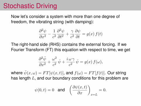
Stochastic DrivingNow let’s consider a system with more than one degree offreedom, the vibrating string (with damping):

∂2ψ

∂x2− 1

c2

∂2ψ

∂t2+γ

c2

∂ψ

∂t= g(x) f(t)

The right-hand side (RHS) contains the external forcing. If weFourier Transform (FT) this equation with respect to time, we get

∂2ψ

∂x2+ω2

c2ψ +

i ω γ

c2ψ = g(x) f(ω),

where ψ(x, ω) = FT [ψ(x, t)], and f(ω) = FT [f(t)]. Our stringhas length L, and our boundary conditions for this problem are

ψ(0, t) = 0 and(∂ψ(x, t)

∂x

)x=L

= 0.

Stochastic Driving

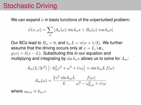
We can expand ψ in basis functions of the unperturbed problem:

ψ(x, ω) =∑n

[An(ω) sin knx+Bn(ω) cos knx]

Our BCs lead to Bn = 0, and kn L = π(n+ 1/2). We furtherassume that the driving occurs only at x = L, i.e.,g(x) = δ(x− L). Substituting this in our equation andmultiplying and integrating by sin knx allows us to solve for Am:

Am(L/2c2)[−k2

mc2 + ω2 + iγω

]= sin kmLf(ω)

Am(ω) =2 c2 sin kmL

L

f(ω)

ω2 − ω20,m + iγω

where ω0,m ≡ km c.

Stochastic DrivingThus, we find that ψ at x = L is

ψ(L, ω) =∑n

c2

2L

f(ω) sin2 knL

ω2 − ω20,n + iγω

=c2

2Lf(ω)

∑n

1

ω2 − ω20,n + iγω

.

The power spectrum of the FT is therefore given by

POWER ≡∣∣ψ(L, ω)

∣∣2∝ |f(ω)|2

∣∣∣∣∣∑n

1

ω2 − ω20,n + iγω

∣∣∣∣∣2

≈ |f(ω)|2∑n

1∣∣∣ω2 − ω20,n + iγω

∣∣∣2

• In the Sun, the driving f(ω) due to the convection zone is a fairlyflat function of ω.

• Although there is power at “all” frequencies (continuous), thediscrete peaks in the power spectrum correspond to the lineareigenfrequencies of the Sun.

A “real” solar spectrum obtained from Doppler observations:

24 CHAPTER 2. ANALYSIS OF OSCILLATION DATA

Figure 2.14: Power spectrum of solar oscillations, obtained from Doppler ob-servations in light integrated over the disk of the Sun. The ordinate is nor-malized to show velocity power per frequency bin. The data were obtainedfrom six observing stations and span approximately four months. Panel (b)provides an expanded view of the central part of the frequency range. Heresome modes have been labelled by their degree l, and the large and smallfrequency separations !! and "!l [cf. equations (2.40) and (2.41)] have beenindicated. (See Elsworth et al. 1995.)

Good News:• “All” the modes in a

broad frequencyrange, with manyvalues of `, areobserved to beexcited in the Sun

Bad News:• The amplitudes are very small. For a given mode, the

flux variations ∆I/I ∼ 10−6, and the velocityvariations are ∼ 15 cm/s

The Sun is so close that these variations are detectable(both from the ground and from space).

In the last 12 years convincing evidence has been foundfor Solar-like oscillations in other stars. The principaldrivers for this progress are the satellite missions COROTand Kepler.

⇒ solar-like oscillations appear to be a generic feature ofstars with convection zones

Asteroseismology — how does it work?

“Using the observed oscillation frequencies of a star to infer itsinterior structure”

• If the structure of our model is “close” to the actualstructure of the star, then the small differencesbetween the observed frequencies and the modelfrequencies give us specific information about theinternal structure of the star

This can be illustrated with a simple physical example:The Vibrating String.

1c2∂2ψ∂t2

= ∂2ψ∂x2 ⇒ ωn = nπc/L, n = 1, 2, 3 . . .

Now perturb the “sound speed” c at the point x, δc(x)

location of perturbation δc(x) ∆ωn ≡ ωn+1 − ωn − πc/L

nL

x = 0.17 L

x = 0.16 L

x = 0.15 L

Pattern of ∆ωn vs n gives location of δc(x)

Amplitude of ∆ωn vs n gives magnitude of δc(x)

How this works mathematically…It can be shown that the string equation,

d2ψ

dx2+ω2

c2ψ = 0,

can be derived from a variational principle for ω2:

ω2[ψ] =

∫ L0dx(dψdx

)2∫ L0dx 1

c2ψ2

.

If ω2[ψ] is an extremum with respect to ψ, then

δω2[ψ] ≡ ω2[ψ + δψ]− ω2[ψ] = 0

∝∫ L

0

dx δψ

(d2ψ

dx2+ω2

c2ψ

).

For δω2 to be zero for arbitrary variations δψ requires that

⇒ d2ψ

dx2+ω2

c2ψ = 0

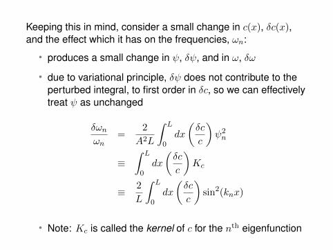
Keeping this in mind, consider a small change in c(x), δc(x),and the effect which it has on the frequencies, ωn:

• produces a small change in ψ, δψ, and in ω, δω

• due to variational principle, δψ does not contribute to theperturbed integral, to first order in δc, so we can effectivelytreat ψ as unchanged

δωnωn

=2

A2L

∫ L

0dx

(δc

c

)ψ2n

≡∫ L

0dx

(δc

c

)Kc

≡ 2

L

∫ L

0dx

(δc

c

)sin2(knx)

• Note: Kc is called the kernel of c for the nth eigenfunction

As an example, if

δc = 0.06L c δ(x−x0),

then we find thefollowingperturbations to thefrequencies:

n (overtone number)

This is because thedifferent modesshow differentsensitivities to theperturbationbecause they havedifferent kernels(eigenfunctions):

Example: specially chosen bumps for the string

(Montgomery 2005, ASP, 334, 553)

The bump/bead introduces “kinks” into the eigenfunctions.Sharp bumps produce larger kinks than broader ones.

Example: specially chosen bumps for the string

The bumps also introduce patterns into the frequencyand/or period spacings:

5 10 15 20 25 30 35 40n (overtone number)

2.5

3.0

3.5

∆ω≡ωn

+1−ωn

Forward Frequency Differences for the Vibrating String

Example: specially chosen bumps for the string

(Montgomery 2005, ASP, 334, 553)

Three beads introduce three “kinks” into the eigenfunctions. Sharpbumps produce larger kinks than broader ones. Note the amplitudedifference across the bumps due to partial reflection of the waves.

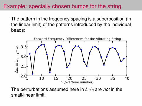
Example: specially chosen bumps for the string

The pattern in the frequency spacing is a superposition (inthe linear limit) of the patterns introduced by the individualbeads:

5 10 15 20 25 30 35 40n (overtone number)

2.0

2.5

3.0

3.5

∆ω≡ωn

+1−ωn

Forward Frequency Differences for the Vibrating String

The perturbations assumed here in δc/c are not in thesmall/linear limit.

Why do we care? Because beads on a stringare like bumps in a stellar model

Changes in thechemical profiles (in aWD) produce bumps inthe Brunt-Väisäläfrequency. Thesebumps produce modetrapping in exactly theyway that beads on astring do. This allows usto learn about thelocation and width ofchemical transitionzones in stars.

Φ ≡ “normalized buoyancy radius” ∝∫ r0dr|N |/r

Mode trapping ofeigenfunctions in a WDmodel due to thecomposition transitionzones.

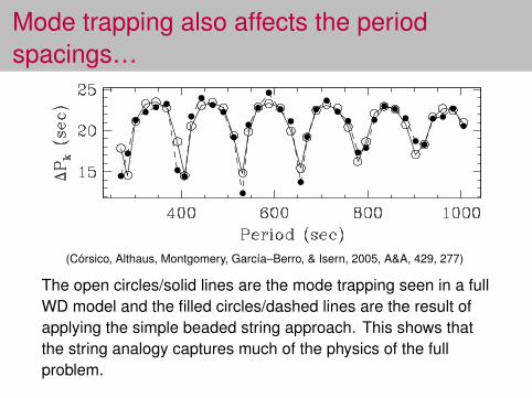
Mode trapping also affects the periodspacings…

(Córsico, Althaus, Montgomery, García–Berro, & Isern, 2005, A&A, 429, 277)

The open circles/solid lines are the mode trapping seen in a fullWD model and the filled circles/dashed lines are the result ofapplying the simple beaded string approach. This shows thatthe string analogy captures much of the physics of the fullproblem.

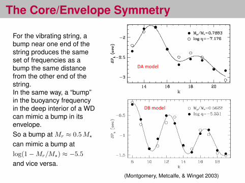
The Core/Envelope Symmetry

For the vibrating string, abump near one end of thestring produces the sameset of frequencies as abump the same distancefrom the other end of thestring.In the same way, a “bump”in the buoyancy frequencyin the deep interior of a WDcan mimic a bump in itsenvelope.So a bump at Mr ≈ 0.5M?

can mimic a bump atlog(1−Mr/M?) ≈ −5.5

and vice versa.

21

DA#model#

DB#model#

(Montgomery, Metcalfe, & Winget 2003)

The Core/Envelope SymmetryWe can map the connection between these “reflection” points,points in the envelope that produce qualitatively the samesignature as points in the core:

"En

vel

op

e M

ass"

"Core Mass"

Observations and Time Series Data

Pulsations are observed by time series measurements of• intensity variations• radial velocity variations

Only for the case of the Sun can we obtain disc-resolvedmeasurements of the perturbations.For other stars, we observe the light integrated over theobserved disc of the star, although the techniques ofDoppler Imaging can be used to provide information aboutthe spatial structure of the perturbations on the stellarsurface.

Sampling and Aliasing

In trying to recover frequencies from data, it is importantfor any gaps in the data to be as small as possible

• This is because data gaps introduce false peaks intothe Fourier transform

• these peaks are called “aliases” of the true frequency• a priori, one cannot tell which peaks are the “true”

peaks and which are the aliases (especially if severalfrequencies are simultaneously present)

For instance, if one observes a star from a singleobservatory, one might obtain 8 hours of data per nightwith a 16-hour gap until the next night’s observations.

Sampling and Aliasing (cont.)

Taking the Fourier Transform of such a signal, we find that

|A(ω)| =

sin[N tD(ω − ω0)/2]

sin[tD(ω − ω0)/2]· sin[tN(ω − ω0)/2]

tN(ω − ω0)/2

where, tD is the length of a day in seconds, tN is the lengthof time observed per night, ω0 is the angular frequency ofthe input signal, and N is the number of nights observed.

The alias structure of a single frequency, sampled in thesame way as the data, is called the “spectral window”, orjust the “window”. The closer this is to a delta function, thebetter.

Sampling and Aliasing (cont.)

five 8-hour nights with16-hour gaps five days continuous data

Sampling and Aliasing (cont.)

Two obvious solutions to this problem:• observe target continuously from space

• SOHO (Solar Heliospheric Observatory)• Kepler satellite

• observe target continuously from the ground…usinga network of observatories

• WET (Whole Earth Telescope)• BISON (Birmingham Solar Oscillations Network)• GONG (Global Oscillations Network Group)

Spectral window for WET observations of the white dwarf GD 358

(Winget, D. E. et al. 1994, ApJ, 430, 839)

Power spectrum of the white dwarf GD 358

(Winget, D. E. et al. 1994, ApJ, 430, 839)

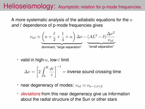
Helioseismology: Asymptotic relation for p-mode frequencies

A more systematic analysis of the adiabatic equations for the nand ` dependence of p-mode frequencies gives

νn` '(n+

`

2+

1

4+ α

)∆ν︸ ︷︷ ︸

dominant, “large separation”

− (AL2 − δ)∆ν2

νn`︸ ︷︷ ︸“small separation”

• valid in high-n, low-` limit

∆ν =

[2

∫ R

0

dr

c

]−1

= inverse sound crossing time

• near degeneracy of modes: νn` ' νn−1,`+2

• deviations from this near degeneracy give us informationabout the radial structure of the Sun or other stars

HelioseismologyHelioseismology is the application of exactly theseprinciples to the oscillations in the Sun:

δωn`ωn`

=

∫ R

0

[Kn`c2δc2

c2+Kn`

ρ

δρ

ρ

]dr

In the above formula, we have defined

δωn` ≡ ωn`(observed)− ωn`(model)δc2 ≡ c2(Sun)− c2(model)δρ ≡ ρ(Sun)− ρ(model)

Kn`c2 ≡ the sampling kernel for c2

for eigenmode n, `Kn`ρ ≡ the sampling kernel for ρ

for eigenmode n, `

Given the large number of observed modes in the Sun (millions,literally), we can hope to construct “locally optimized kernels” bylooking at the appropriate linear combinations of the frequencydifferences, δωn`:∑

n,`

An`δωn`ωn`

=

∫ R

0

[δc2

c2

∑n,`

An`Kn`c2︸ ︷︷ ︸

≡Kopt

c2

+δρ

ρ

∑n,`

An`Kn`ρ︸ ︷︷ ︸

≡Koptρ

]dr

Since the original kernels are oscillatory, such as individualterms in a Fourier series, by choosing the Ai appropriatelywe can make the optimized kernels, Kopt

x have any functionalform we choose. In particular, …

InversionsThe An` can be chosen such that

• Koptc2 is strongly peaked at r = 0.75R, say

• Koptρ is negligibly small everywhere (is suppressed)

The result: a helioseismic inversion for the sound speed in the Sun

The most conspicuous feature of this inversion is thebump at r ∼ 0.65R, where

δc2 ≡ c2(Sun)− c2(model)

• most likely explanation has to do with He settling(diffusion)

• the model includes He settling, which enhances theHe concentration in this region

• overshooting of the convection zone may inhibit Hesettling

⇒ Sun has lower He concentration than model at thispoint

• since c2 ∝ Γ1T/µ, and model has higher µ than Sun,this produces a positive bump in δc2

Why do inversions work so well for solarp-modes?

• solar p-modes can be thought ofas sound waves which refract offthe deeper layers

• depth of penetration depends on `

low-`: penetrate deeply, samplethe core

high-`: do not penetrate deeply,sample only the envelope

⇒ different `’s are very linearly independent

⇒ relatively easy to construct localized kernels

Refraction of p-modes• p-modes are essentially sound waves• c2

s ∼ kBT/m⇒ c2

s is a decreasing function of r• wavefront is refracted upward

• “mirage” or “hot road” effect

Major Results of Helioseismology

• depth of the convection zone measured• found to be ∼ 3 times deeper than previously thought

(models in the 1970’s had been “tweaked” to minimizethe Solar neutrino problem)

In addition, Houdek and Gough (2007, MNRAS, 375, 861)have recently shown that, by looking at seconddifferences of low-` modes only, one could derive thedepth of the convection zone:

Major Results of Helioseismology (cont.)(∆2ν ≡ νn+1,` − 2 νn,` + νn−1,`)

12 G.Houdek & D.O.Gough

Figure 11. Top: The symbols are second di!erences "2!, definedby equation (2), of low-degree (l=0,1,2) eigenfrequencies obtainedfrom adiabatic pulsation calculations of the central model 0, andhave the same relation to l as in Fig. 1. The solid curve is thediagnostic D2 determined by equations (21), (30) & (37), whoseeleven parameters "k have been adjusted to fit the data by leastsquares. The measure #2 (mean squared di!erences) of the over-all misfit is (53 nHz)2. The dashed curve represents the smoothcontribution (last term in equation (21)). Bottom: Individual con-tributions of the oscillatory seismic diagnostic. The solid curvedisplays the He II contribution, the dotted curve is the He I con-tribution and the dot-dashed curve is the contribution from thebase of the convection zone.

within the He I ionization zone (in the case of the Sun andsimilar stars, this is not the case of He II ionization), and theevanescence of the eigenfunction above the turning pointmust be taken into account. This can be achieved via theusual Airy-function representation. But for the purpose ofevaluating the integral !!K it is adequate simply to use theappropriate high-|"| sinusoidal or exponential asymptoticrepresentations either side of the turning point to estimatethe ‘oscillatory’ component of the integrand, which amountsto setting

[(div#)2]osc ! " $3

2%pcr2&cos 2" , for ' > 't , (34)

with " given by equation (27), without the subscripts II,and & by equation (26). Despite the vanishing of & at' = 't = (m + 1)/$, expression (34) is finite at ' = 'tbecause 2"('t) = (/2. One can treat the evanescent regionsimilarly, avoiding the singularity and making the represen-tation continuous at ' = 't by writing

[(div#)]2osc ! " $3

2%pcr2|&| (1 " e2"!#/2) , for ' < 't , (35)

Figure 12. Top: The symbols (with error bars computed underthe assumption that the raw frequency errors are independent)represent second di!erences "2!, defined by equation (2), of low-degree solar frequencies with l=0,1,2 and 3, obtained from Bi-SON (Basu et al. 2006). The e!ective overall error in the data is!$" =5.3 nHz. The solid curve is the diagnostic D2(!;"k), whichhas been fitted to the data in a manner intended to provide an op-timal estimate of the eleven parameters "k . The values of someof these fitting parameters are: #%&/&|$II $ 0.047, 'II $ 819 s,"II $ 70 s, and the measure E of the overall misfit is 33 nHz.The direct measure # is 2.1; the minimum-#2 fit of the functionD2 to the data yields #min = 1.6. The dashed curve representsthe smooth contribution (last term in equation (21)). Bottom: In-dividual contributions of the seismic diagnostic. The solid curvedisplays the He II contribution, the dotted curve is the He I con-tribution and the dot-dashed curve is the contribution from the

base of the convection zone.

where now

"(' ) ! |&|'$ " (m + 1) ln

„

m + 1

'$+ |&|

«

+(

4. (36)

Although this expression has the wrong magnitude where"" is large, that region makes very little contribution tothe integral for !!K. We have confirmed numerically thatthe formula (35) provides a tolerable approximation. At anypoint the integrand for !!K is the product of an exponentialand a slowly varying function F (' ), say. Both F (' ) and "(' )can be Taylor expanded about ' = 'I = 'I + $!1)I ()I =)II) up to the quadratic term, rendering the approximationasymptotically integrable in closed form. The correction tothe result of assuming F (' ) = F ('I) and " = "I is small, sowe actually adopt just the leading term.

The cyclic-eigenfrequency contribution to the entire he-lium glitch then becomes

!!* ! AII

ˆ

* + 12(m + 1)*0

˜

12 G.Houdek & D.O.Gough

Figure 11. Top: The symbols are second di!erences "2!, definedby equation (2), of low-degree (l=0,1,2) eigenfrequencies obtainedfrom adiabatic pulsation calculations of the central model 0, andhave the same relation to l as in Fig. 1. The solid curve is thediagnostic D2 determined by equations (21), (30) & (37), whoseeleven parameters "k have been adjusted to fit the data by leastsquares. The measure #2 (mean squared di!erences) of the over-all misfit is (53 nHz)2. The dashed curve represents the smoothcontribution (last term in equation (21)). Bottom: Individual con-tributions of the oscillatory seismic diagnostic. The solid curvedisplays the He II contribution, the dotted curve is the He I con-tribution and the dot-dashed curve is the contribution from thebase of the convection zone.

within the He I ionization zone (in the case of the Sun andsimilar stars, this is not the case of He II ionization), and theevanescence of the eigenfunction above the turning pointmust be taken into account. This can be achieved via theusual Airy-function representation. But for the purpose ofevaluating the integral !!K it is adequate simply to use theappropriate high-|"| sinusoidal or exponential asymptoticrepresentations either side of the turning point to estimatethe ‘oscillatory’ component of the integrand, which amountsto setting

[(div#)2]osc ! " $3

2%pcr2&cos 2" , for ' > 't , (34)

with " given by equation (27), without the subscripts II,and & by equation (26). Despite the vanishing of & at' = 't = (m + 1)/$, expression (34) is finite at ' = 'tbecause 2"('t) = (/2. One can treat the evanescent regionsimilarly, avoiding the singularity and making the represen-tation continuous at ' = 't by writing

[(div#)]2osc ! " $3

2%pcr2|&| (1 " e2"!#/2) , for ' < 't , (35)

Figure 12. Top: The symbols (with error bars computed underthe assumption that the raw frequency errors are independent)represent second di!erences "2!, defined by equation (2), of low-degree solar frequencies with l=0,1,2 and 3, obtained from Bi-SON (Basu et al. 2006). The e!ective overall error in the data is!$" =5.3 nHz. The solid curve is the diagnostic D2(!;"k), whichhas been fitted to the data in a manner intended to provide an op-timal estimate of the eleven parameters "k . The values of someof these fitting parameters are: #%&/&|$II $ 0.047, 'II $ 819 s,"II $ 70 s, and the measure E of the overall misfit is 33 nHz.The direct measure # is 2.1; the minimum-#2 fit of the functionD2 to the data yields #min = 1.6. The dashed curve representsthe smooth contribution (last term in equation (21)). Bottom: In-dividual contributions of the seismic diagnostic. The solid curvedisplays the He II contribution, the dotted curve is the He I con-tribution and the dot-dashed curve is the contribution from the

base of the convection zone.

where now

"(' ) ! |&|'$ " (m + 1) ln

„

m + 1

'$+ |&|

«

+(

4. (36)

Although this expression has the wrong magnitude where"" is large, that region makes very little contribution tothe integral for !!K. We have confirmed numerically thatthe formula (35) provides a tolerable approximation. At anypoint the integrand for !!K is the product of an exponentialand a slowly varying function F (' ), say. Both F (' ) and "(' )can be Taylor expanded about ' = 'I = 'I + $!1)I ()I =)II) up to the quadratic term, rendering the approximationasymptotically integrable in closed form. The correction tothe result of assuming F (' ) = F ('I) and " = "I is small, sowe actually adopt just the leading term.

The cyclic-eigenfrequency contribution to the entire he-lium glitch then becomes

!!* ! AII

ˆ

* + 12(m + 1)*0

˜

rC/R ' 0.7

Major Results of Helioseismology (cont.)

• the standard opacities used up to the late 1980’swere found to be ∼ 3 too smallthe effects of metals needed to be added

• this led to the:OPAL opacity project (Iglesias & Rogers 1996, ApJ,464, 943)OP opacity project (Seaton et al. 1994, MNRAS, 266,805)

• this had effects throughout the H-R diagram:e.g., with new higher opacities, the pulsations of Bstars could now be explained (bump in opacity due topartial ionization of metals — Dziembowski &Pamyatnykh 1993, MNRAS, 262, 204)

Major Results of Helioseismology (cont.)

• detection of differential rotation in the Sun• rotation profile different from what was theoretically

expected

• discovery of a shear layer near the base of the Solarconvection zone (the “tachocline”)

Both of these effects have to do with rotation.

How does rotation affect a pulsating object?

The Effect of Rotation

• breaks spherical symmetry• analogous to an H atom in an external magnetic field

• lifts degeneracy of frequencies of modes with thesame n, ` but different m

• again analogous to an H atom (Zeeman splitting)

• frequencies are perturbed by the non-zero fluidvelocities of the equilibrium state (e.g., to linear orderby the “Coriolis force” and to second order by the“centrifugal force”)

The Effect of Rotation (cont.)

• if rotation may be treated as a perturbation (“slowrotation”), then we can calculate kernels which give thefrequency perturbations as an average over the rotationprofile Ω(r, θ):

δωn`m =

∫ R

0dr

∫ π

0rdθKn`m(r, θ) Ω(r, θ)

• for uniform (“solid body”) rotation

δωn`m = mβn` Ωsolid

⇒ δω is linearly proportional to m, the azimuthalquantum number

• for more general (differential) rotation, e.g., Ω = Ω(r, θ), δωis no longer a linear function of m

⇒ departures from linearity give information aboutΩ(r, θ)

Rotational Inversion for the Sun

• radiative interiorrotates rigidly

• convection zonerotatesdifferentially

• faster atequator

• slower atpoles

nHz

radiative convective

• naive models predict “constant rotation on cylinders”• in contrast, in the convective region, we find that the

rotation rate is mainly a function of latitude, Ω ≈ Ω(θ)⇒ little radial shear in the convection zone

• nearly rigid rotation of radiative region impliesadditional processes are at work

• e.g., a magnetic field could help these layers to rotaterigidly

• The tachocline: the region of shear between therigidly rotating radiative region and the differentiallyrotating convective region

The Solar Tachocline

(from Charbonneau et al. 1999, Apj, 527, 445)

• location: r ≈ 0.70R• thickness: w ≈ 0.04R• prolate in shape:

rt ≈ 0.69R (equator)rt ≈ 0.71R (latitude 60)

• likely seat for the Solar dynamo• magnetic field + shear

Rotation in Red Giants

LETTERdoi:10.1038/nature10612

Fast core rotation in red-giant stars as revealed bygravity-dominated mixed modesPaul G. Beck1, Josefina Montalban2, Thomas Kallinger1,3, Joris De Ridder1, Conny Aerts1,4, Rafael A. Garcıa5, Saskia Hekker6,7,Marc-Antoine Dupret2, Benoit Mosser8, Patrick Eggenberger9, Dennis Stello10, Yvonne Elsworth7, Søren Frandsen11,Fabien Carrier1, Michel Hillen1, Michael Gruberbauer12, Jørgen Christensen-Dalsgaard11, Andrea Miglio7, Marica Valentini2,Timothy R. Bedding10, Hans Kjeldsen11, Forrest R. Girouard13, Jennifer R. Hall13 & Khadeejah A. Ibrahim13

When the core hydrogen is exhausted during stellar evolution, thecentral region of a star contracts and the outer envelope expands andcools, giving rise to a red giant. Convection takes place over much ofthe star’s radius. Conservation of angular momentum requires thatthe cores of these stars rotate faster than their envelopes; indirectevidence supports this1,2. Information about the angular-momentumdistribution is inaccessible to direct observations, but it can beextracted from the effect of rotation on oscillation modes that probethe stellar interior. Here we report an increasing rotation rate fromthe surface of the star to the stellar core in the interiors of red giants,obtained using the rotational frequency splitting of recently detected‘mixed modes’3,4. By comparison with theoretical stellar models, weconclude that the core must rotate at least ten times faster than thesurface. This observational result confirms the theoretical predictionof a steep gradient in the rotation profile towards the deep stellarinterior1,5,6.

The asteroseismic approach to studying stellar interiors exploitsinformation from oscillation modes of different radial order n andangular degree l, which propagate in cavities extending at differentdepths7. Stellar rotation lifts the degeneracy of non-radial modes, pro-ducing a multiplet of (2l 1 1) frequency peaks in the power spectrum foreach mode. The frequency separation between two mode componentsof a multiplet is related to the angular velocity and to the properties ofthe mode in its propagation region. More information on the exploita-tion of rotational splitting of modes may be found in the SupplementaryInformation. An important new tool comes from mixed modes thatwere recently identified in red giants3,4. Stochastically excited solar-likeoscillations in evolved G and K giant stars8 have been well studied interms of theory9–12, and the main results are consistent with recentobservations from space-based photometry13,14. Whereas pressuremodes are completely trapped in the outer acoustic cavity, mixed modesalso probe the central regions and carry additional information from thecore region, which is probed by gravity modes. Mixed dipole modes(l 5 1) appear in the Fourier power spectrum as dense clusters of modesaround those that are best trapped in the acoustic cavity. These clusters,the components of which contain varying amounts of influence frompressure and gravity modes, are referred to as ‘dipole forests’.

We present the Fourier spectra of the brightness variations of starsKIC 8366239 (Fig. 1a), KIC 5356201 (Supplementary Fig. 3a) and KIC12008916 (Supplementary Fig. 5a), derived from observations with theKepler spacecraft. The three spectra show split modes, the sphericaldegree of which we identify as l 5 1. These detected multiplets cannothave been caused by finite mode lifetime effects from mode damping,

because that would not lead to a consistent multiplet appearance overseveral orders such as that shown in Fig. 1. The spacings in periodbetween the multiplet components (Supplementary Fig. 7) are toosmall to be attributable to consecutive unsplit mixed modes4 and donot follow the characteristic frequency pattern of unsplit mixedmodes3. Finally, the projected surface velocity, v sin i, obtained fromground-based spectroscopy (Table 1), is consistent with the rotationalvelocity measured from the frequency splitting of the mixed mode thatpredominantly probes the outer layers. We are thus left with rotationas the only cause of the detected splittings.

The observed rotational splitting is not constant for consecutivedipole modes, even within a given dipole forest (Fig. 1b and Sup-plementary Figs 3b and 5b). The lowest splitting is generally presentfor the mode at the centre of the dipole forest, which is the mode withthe largest amplitude in the outer layers. Splitting increases for modeswith a larger gravity component, towards the wings of the dipole modeforest. For KIC 8366239, we find that the average splitting of modes inthe wings of the dipole forests is 1.5 times larger than the mean splittingof the centre modes of the dipole forests.

We compared the observations (Fig. 1b) with theoretical predictionsfor a model representative of KIC 8366239, as defined in the Sup-plementary Information. The effect of rotation on the oscillationfrequencies can be estimated in terms of a weight function, called arotational kernel (Knl). From the kernels, it is shown that at least 60% ofthe frequency splitting for the l 5 1 mixed modes with a dominantgravity component is produced in the central region of the star (Fig. 2).This substantial core contribution to mixed modes enables us toinvestigate the rotational properties of the core region, which washitherto not possible for the Sun, owing to a lack of observed modesthat probe the core region (within a radius r , 0.2 R[; ref. 15). Thesolar rotational profile is known in great detail for only those regionsprobed by pressure-dominated modes16–18. In contrast to these modesin the wings of the dipole forest, only 30% of the splitting of the centremode originates from the central region of the star, whereas the outerthird by mass of the star contributes 50% of the frequency splitting. Bycomparing the rotational velocity derived from the splitting of suchpressure-dominated modes with the projected surface velocity fromspectroscopy, we find that the asteroseismic value is systematicallylarger. This offset cannot be explained by inclination of the rotationaxis towards the observer alone (Supplementary Tables 1 and 2), butoriginates from the contribution of the fast-rotating core (Fig. 2).Furthermore, internal non-rigid rotation leads to a larger splittingfor modes in the wings of the dipole forest than for centre modes.

1Instituut voor Sterrenkunde, Katholieke Universiteit Leuven, 3001 Leuven, Belgium. 2Institut d’Astrophysique et de Geophysique de l’Universite de Liege, 4000 Liege, Belgium. 3Institut fur Astronomie derUniversitat Wien, Turkenschanzstraße 17, 1180 Wien, Austria. 4Afdeling Sterrenkunde, Institute for Mathematics Astrophysics and Particle Physics (IMAPP), Radboud University Nijmegen, 6500GLNijmegen, The Netherlands. 5Laboratoire Astrophysique, Instrumentation et Modelisation (AIM), CEA/DSM—CNRS—Universite Paris Diderot; Institut de Recherche sur les lois Fondamentales de l’Univers/Service d’Astrophysique (IRFU/Sap), Centre de Saclay, 91191 Gif-sur-Yvette Cedex, France. 6Astronomical Institute ’Anton Pannekoek’, University of Amsterdam, Science Park 904, 1098 XH Amsterdam,The Netherlands. 7School of Physics and Astronomy, University of Birmingham, Edgbaston, Birmingham B15 2TT, UK. 8Laboratoire d’etudes spatiales et d’instrumentation (LESIA), CNRS, Universite Pierreet Marie Curie, Universite Denis Diderot, Observatoire de Paris, 92195 Meudon Cedex, France. 9Observatoire de Geneve, Universite de Geneve, 51 Ch. des Maillettes, 1290 Sauverny, Switzerland. 10SydneyInstitute for Astronomy (SIfA), School of Physics, University of Sydney 2006, Australia. 11Department of Physics and Astronomy, Aarhus University, DK-8000 Aarhus C, Denmark. 12Department ofAstronomy and Physics, Saint Marys University, Halifax, NS B3H 3C3, Canada. 13Orbital Sciences Corporation/NASA Ames Research Center, Moffett Field, 94035 California, USA.

5 J A N U A R Y 2 0 1 2 | V O L 4 8 1 | N A T U R E | 5 5

Macmillan Publishers Limited. All rights reserved©2012

Rotation in Red Giants

Supplementary Figure 8. The value βnl and mode inertia for a representative stellar model

of KIC 8366239. a, βnl as a function of mode frequency for oscillation modes of spherical degree

ℓ=1 and ℓ=2 b, The corresponding mode inertia log(E) of these modes. Modes of degree ℓ=0,

ℓ=1, ℓ=2 are drawn in green, blue, and red, respectively.

SUPPLEMENTARY INFORMATIONRESEARCHdoi:10.1038/nature10612

WWW.NATURE.COM/ NATURE | 16

Supplementary Figure 8. The value βnl and mode inertia for a representative stellar model

of KIC 8366239. a, βnl as a function of mode frequency for oscillation modes of spherical degree

ℓ=1 and ℓ=2 b, The corresponding mode inertia log(E) of these modes. Modes of degree ℓ=0,

ℓ=1, ℓ=2 are drawn in green, blue, and red, respectively.

SUPPLEMENTARY INFORMATIONRESEARCHdoi:10.1038/nature10612

WWW.NATURE.COM/ NATURE | 16

Rotation in Red Giants

A&A 548, A10 (2012)DOI: 10.1051/0004-6361/201220106c! ESO 2012

Astronomy&

Astrophysics

Spin down of the core rotation in red giants!

B. Mosser1, M. J. Goupil1, K. Belkacem1, J. P. Marques2, P. G. Beck3, S. Bloemen3, J. De Ridder3, C. Barban1,S. Deheuvels4, Y. Elsworth5, S. Hekker6,5, T. Kallinger3, R. M. Ouazzani7,1, M. Pinsonneault8, R. Samadi1, D. Stello9,

R. A. García10, T. C. Klaus11, J. Li12, S. Mathur13, and R. L. Morris12

1 LESIA, CNRS, Université Pierre et Marie Curie, Université Denis Diderot, Observatoire de Paris, 92195 Meudon Cedex, Francee-mail: benoit.mosser@obspm.fr

2 Georg-August-Universität Göttingen, Institut für Astrophysik, Friedrich-Hund-Platz 1, 37077 Göttingen, Germany3 Instituut voor Sterrenkunde, K. U. Leuven, Celestijnenlaan 200D, 3001 Leuven, Belgium4 Department of Astronomy, Yale University, PO Box 208101, New Haven, CT 06520-8101, USA5 School of Physics and Astronomy, University of Birmingham, Edgbaston, Birmingham B15 2TT, UK6 Astronomical Institute ‘Anton Pannekoek’, University of Amsterdam, Science Park 904, 1098 XH Amsterdam, The Netherlands7 Institut d’Astrophysique et de Géophysique de l’Université de Liège, Allée du 6 Août 17, 4000 Liège, Belgium8 Department of Astronomy, The Ohio State University, Columbus, OH 43210, USA9 Sydney Institute for Astronomy, School of Physics, University of Sydney, NSW 2006, Australia

10 Laboratoire AIM, CEA/DSM CNRS – Université Denis Diderot IRFU/SAp, 91191 Gif-sur-Yvette Cedex, France11 Orbital Sciences Corporation/NASA Ames Research Center, Mo!ett Field, CA 94035, USA12 SETI Institute/NASA Ames Research Center, Mo!ett Field, CA 94035, USA13 High Altitude Observatory, NCAR, PO Box 3000, Boulder, CO 80307, USA

Received 26 July 2012 / Accepted 13 September 2012

ABSTRACT

Context. The space mission Kepler provides us with long and uninterrupted photometric time series of red giants. We are now able toprobe the rotational behaviour in their deep interiors using the observations of mixed modes.Aims. We aim to measure the rotational splittings in red giants and to derive scaling relations for rotation related to seismic andfundamental stellar parameters.Methods. We have developed a dedicated method for automated measurements of the rotational splittings in a large number of redgiants. Ensemble asteroseismology, namely the examination of a large number of red giants at di!erent stages of their evolution,allows us to derive global information on stellar evolution.Results. We have measured rotational splittings in a sample of about 300 red giants. We have also shown that these splittings aredominated by the core rotation. Under the assumption that a linear analysis can provide the rotational splitting, we observe a smallincrease of the core rotation of stars ascending the red giant branch. Alternatively, an important slow down is observed for red-clumpstars compared to the red giant branch. We also show that, at fixed stellar radius, the specific angular momentum increases withincreasing stellar mass.Conclusions. Ensemble asteroseismology indicates what has been indirectly suspected for a while: our interpretation of the observedrotational splittings leads to the conclusion that the mean core rotation significantly slows down during the red giant phase. The slow-down occurs in the last stages of the red giant branch. This spinning down explains, for instance, the long rotation periods measuredin white dwarfs.

Key words. stars: oscillations – stars: interiors – stars: rotation – stars: late-type

1. Introduction

The internal structure of red giants bears the history of their evo-lution. They are therefore seen as key for the understanding ofstellar evolution. They are expected to have a rapidly rotatingcore and a slowly rotating envelope (e.g. Sills & Pinsonneault2000), as a result of internal angular momentum distribution.Indirect indications of the internal angular momentum are givenby surface-abundance anomalies resulting from the action ofinternal transport processes and from the redistribution of an-gular momentum and chemical elements (Zahn 1992; Talon &Charbonnel 2008; Maeder 2009; Canto Martins et al. 2011).Direct measurements of the surface rotation are given by themeasure of v sin i (e.g. Carney et al. 2008). The slow rotation

! Appendices A and B are available in electronic form athttp://www.aanda.org

rate in low-mass white dwarfs (e.g. Kawaler et al. 1999) sug-gests a spinning down of the rotation during the red giant branch(RGB) phase. In addition, 3D simulations show non-rigid rota-tion in the convective envelope of red giants (Brun & Palacios2009). Di!erent mechanisms for spinning down the core havebeen investigated (e.g. Charbonnel & Talon 2005). Rotationally-induced mixing, amid other angular momentum transport mech-anisms, is still poorly understood but is known to take place instellar interiors. Therefore, a direct measurement of rotation in-side red giants would give us an unprecedented opportunity toperform a leap forward on our understanding of angular mo-mentum transport in stellar interiors (e.g. Lagarde et al. 2012;Eggenberger et al. 2012).

This is becoming possible with seismology, which providesus with direct access to measure the internal rotation profile, asshown by Beck et al. (2012) and Deheuvels et al. (2012a). They

Article published by EDP Sciences A10, page 1 of 14

A&A 548, A10 (2012)DOI: 10.1051/0004-6361/201220106c! ESO 2012

Astronomy&

Astrophysics

Spin down of the core rotation in red giants!

B. Mosser1, M. J. Goupil1, K. Belkacem1, J. P. Marques2, P. G. Beck3, S. Bloemen3, J. De Ridder3, C. Barban1,S. Deheuvels4, Y. Elsworth5, S. Hekker6,5, T. Kallinger3, R. M. Ouazzani7,1, M. Pinsonneault8, R. Samadi1, D. Stello9,

R. A. García10, T. C. Klaus11, J. Li12, S. Mathur13, and R. L. Morris12

1 LESIA, CNRS, Université Pierre et Marie Curie, Université Denis Diderot, Observatoire de Paris, 92195 Meudon Cedex, Francee-mail: benoit.mosser@obspm.fr

2 Georg-August-Universität Göttingen, Institut für Astrophysik, Friedrich-Hund-Platz 1, 37077 Göttingen, Germany3 Instituut voor Sterrenkunde, K. U. Leuven, Celestijnenlaan 200D, 3001 Leuven, Belgium4 Department of Astronomy, Yale University, PO Box 208101, New Haven, CT 06520-8101, USA5 School of Physics and Astronomy, University of Birmingham, Edgbaston, Birmingham B15 2TT, UK6 Astronomical Institute ‘Anton Pannekoek’, University of Amsterdam, Science Park 904, 1098 XH Amsterdam, The Netherlands7 Institut d’Astrophysique et de Géophysique de l’Université de Liège, Allée du 6 Août 17, 4000 Liège, Belgium8 Department of Astronomy, The Ohio State University, Columbus, OH 43210, USA9 Sydney Institute for Astronomy, School of Physics, University of Sydney, NSW 2006, Australia

10 Laboratoire AIM, CEA/DSM CNRS – Université Denis Diderot IRFU/SAp, 91191 Gif-sur-Yvette Cedex, France11 Orbital Sciences Corporation/NASA Ames Research Center, Mo!ett Field, CA 94035, USA12 SETI Institute/NASA Ames Research Center, Mo!ett Field, CA 94035, USA13 High Altitude Observatory, NCAR, PO Box 3000, Boulder, CO 80307, USA

Received 26 July 2012 / Accepted 13 September 2012

ABSTRACT

Context. The space mission Kepler provides us with long and uninterrupted photometric time series of red giants. We are now able toprobe the rotational behaviour in their deep interiors using the observations of mixed modes.Aims. We aim to measure the rotational splittings in red giants and to derive scaling relations for rotation related to seismic andfundamental stellar parameters.Methods. We have developed a dedicated method for automated measurements of the rotational splittings in a large number of redgiants. Ensemble asteroseismology, namely the examination of a large number of red giants at di!erent stages of their evolution,allows us to derive global information on stellar evolution.Results. We have measured rotational splittings in a sample of about 300 red giants. We have also shown that these splittings aredominated by the core rotation. Under the assumption that a linear analysis can provide the rotational splitting, we observe a smallincrease of the core rotation of stars ascending the red giant branch. Alternatively, an important slow down is observed for red-clumpstars compared to the red giant branch. We also show that, at fixed stellar radius, the specific angular momentum increases withincreasing stellar mass.Conclusions. Ensemble asteroseismology indicates what has been indirectly suspected for a while: our interpretation of the observedrotational splittings leads to the conclusion that the mean core rotation significantly slows down during the red giant phase. The slow-down occurs in the last stages of the red giant branch. This spinning down explains, for instance, the long rotation periods measuredin white dwarfs.

Key words. stars: oscillations – stars: interiors – stars: rotation – stars: late-type

1. Introduction

The internal structure of red giants bears the history of their evo-lution. They are therefore seen as key for the understanding ofstellar evolution. They are expected to have a rapidly rotatingcore and a slowly rotating envelope (e.g. Sills & Pinsonneault2000), as a result of internal angular momentum distribution.Indirect indications of the internal angular momentum are givenby surface-abundance anomalies resulting from the action ofinternal transport processes and from the redistribution of an-gular momentum and chemical elements (Zahn 1992; Talon &Charbonnel 2008; Maeder 2009; Canto Martins et al. 2011).Direct measurements of the surface rotation are given by themeasure of v sin i (e.g. Carney et al. 2008). The slow rotation

! Appendices A and B are available in electronic form athttp://www.aanda.org

rate in low-mass white dwarfs (e.g. Kawaler et al. 1999) sug-gests a spinning down of the rotation during the red giant branch(RGB) phase. In addition, 3D simulations show non-rigid rota-tion in the convective envelope of red giants (Brun & Palacios2009). Di!erent mechanisms for spinning down the core havebeen investigated (e.g. Charbonnel & Talon 2005). Rotationally-induced mixing, amid other angular momentum transport mech-anisms, is still poorly understood but is known to take place instellar interiors. Therefore, a direct measurement of rotation in-side red giants would give us an unprecedented opportunity toperform a leap forward on our understanding of angular mo-mentum transport in stellar interiors (e.g. Lagarde et al. 2012;Eggenberger et al. 2012).

This is becoming possible with seismology, which providesus with direct access to measure the internal rotation profile, asshown by Beck et al. (2012) and Deheuvels et al. (2012a). They

Article published by EDP Sciences A10, page 1 of 14

Rotation in Red GiantsB. Mosser et al.: Rotation in red giants

Fig. 9. Mean period of core rotation as a function of the asteroseismic stellar radius, in log-log scale. Same symbols and color code as in Fig. 6. Thedotted line indicates a rotation period varying as R2. The dashed (dot-dashed, triple-dot-dashed) line indicates the fit of RGB (clump, secondaryclump) core rotation period. The rectangles in the right side indicate the typical error boxes, as a function of the rotation period.

momentum is certainly transferred from the core to the envelope,in order to spin down the core. However, a strong di!erential ro-tation profile takes place when giants ascend the RGB (Marqueset al. 2012; Goupil et al. 2012).

6.1.2. Clump stars

The extrapolation of the fit reported by Eq. (26) to a typical stel-lar radius at the red clump shows that cores of clump stars arerotating six times slower. This slower rotation can be partly ex-plained by the core radius change occurring when helium fusionignition removes the degeneracy in the core. This change, esti-mated to be less than 50% (Sills & Pinsonneault 2000), can how-ever not be responsible for an increase of the mean core rotationperiod as large as a factor of six. As a consequence, the slowerrotation observed in clump stars indicates that internal angularmomentum has been transferred from the rapidly rotating coreto the slowly rotating envelope (Fig. 9).

6.1.3. Comparison with modeling

The comparison with modeling reinforces this view (Fig. 1 ofSills & Pinsonneault 2000). Their evolution model assumes alocal conservation of angular momentum in radiative regions andsolid-body rotation in convective regions. It provides values forthe core rotation in a 0.8 M! star of about 50 days on the mainsequence, about 2 days on the RGB at the position of maximumconvection zone depth in mass, and about 7 days in the clump.This means that, even in a case where the initial rotation on themain-sequence is slow (certainly much slower than the main-sequence progenitors of the red giants studied here) and whereangular momentum is massively transferred in order to insurethat convective regions rotate rigidly, the predicted core rotationperiods are much smaller than observed. The expansion of theconvective envelope provides favorable conditions for internalgravity waves to transfer internal momentum from the core tothe envelope to spin down the core rotation (Zahn et al. 1997;Mathis 2009). Talon & Charbonnel (2008) have shown that the

conditions are favorable for these waves to operate at the end ofthe subgiant branch and during the early-AGB phase. There isobservational evidence that the spinning down should have beenboosted in the upper RGB too.

The comparison of the core rotation evolution on the RGBand in the clump shows that the angular momentum transfer isnot enough for erasing the di!erential rotation in clump stars.The line representing an evolution of "Trot#c with R2 extrapo-lated to typical main-sequence stellar radii gives a much morerapid core rotation than the extrapolation from the RGB fit. Thisindicates that the interior structure of a red-clump star has to sus-tain, despite the spinning down of the core rotation, a significantdi!erential rotation. This conclusion, implicitly based on the as-sumption of total angular momentum conservation, is reinforcedin case of total spinning down at the tip of the RGB. However,the large similarities of the values of the core rotation period ob-served in clump stars, together with an evolution of "Trot#c closeto R2 (Eq. (27)), should imply that a regime is found with a corerotation of clump stars much more rapid than the envelope rota-tion but closely linked to it.

6.2. Mass dependence

We have calculated, for di!erent mass ranges [M1,M2], a meancore rotation period defined by

""Trot#c#[M1,M2] =

!M2M1"Trot#c R$r

!M2M1

R$r(29)

where r is the exponent given by Eqs. (26) or (27), depending onthe evolutionary status.

This expression allows us to derive a mean value even forRGB stars, in the mass range [1.2, 1.5 M!] where the RGB starsample can be considered as unbiased. We do not detect anymass dependence. The situation changes drastically for clumpstars, with a clear mass dependence: the mean value of "Trot#c isdivided by a factor of about 1.7 from 1 to 2 M!. This reinforcesthe view that angular momentum is certainly exchanged in the

A10, page 9 of 14

B. Mosser et al.: Rotation in red giants

Fig. 9. Mean period of core rotation as a function of the asteroseismic stellar radius, in log-log scale. Same symbols and color code as in Fig. 6. Thedotted line indicates a rotation period varying as R2. The dashed (dot-dashed, triple-dot-dashed) line indicates the fit of RGB (clump, secondaryclump) core rotation period. The rectangles in the right side indicate the typical error boxes, as a function of the rotation period.

momentum is certainly transferred from the core to the envelope,in order to spin down the core. However, a strong di!erential ro-tation profile takes place when giants ascend the RGB (Marqueset al. 2012; Goupil et al. 2012).

6.1.2. Clump stars

The extrapolation of the fit reported by Eq. (26) to a typical stel-lar radius at the red clump shows that cores of clump stars arerotating six times slower. This slower rotation can be partly ex-plained by the core radius change occurring when helium fusionignition removes the degeneracy in the core. This change, esti-mated to be less than 50% (Sills & Pinsonneault 2000), can how-ever not be responsible for an increase of the mean core rotationperiod as large as a factor of six. As a consequence, the slowerrotation observed in clump stars indicates that internal angularmomentum has been transferred from the rapidly rotating coreto the slowly rotating envelope (Fig. 9).

6.1.3. Comparison with modeling

The comparison with modeling reinforces this view (Fig. 1 ofSills & Pinsonneault 2000). Their evolution model assumes alocal conservation of angular momentum in radiative regions andsolid-body rotation in convective regions. It provides values forthe core rotation in a 0.8 M! star of about 50 days on the mainsequence, about 2 days on the RGB at the position of maximumconvection zone depth in mass, and about 7 days in the clump.This means that, even in a case where the initial rotation on themain-sequence is slow (certainly much slower than the main-sequence progenitors of the red giants studied here) and whereangular momentum is massively transferred in order to insurethat convective regions rotate rigidly, the predicted core rotationperiods are much smaller than observed. The expansion of theconvective envelope provides favorable conditions for internalgravity waves to transfer internal momentum from the core tothe envelope to spin down the core rotation (Zahn et al. 1997;Mathis 2009). Talon & Charbonnel (2008) have shown that the

conditions are favorable for these waves to operate at the end ofthe subgiant branch and during the early-AGB phase. There isobservational evidence that the spinning down should have beenboosted in the upper RGB too.

The comparison of the core rotation evolution on the RGBand in the clump shows that the angular momentum transfer isnot enough for erasing the di!erential rotation in clump stars.The line representing an evolution of "Trot#c with R2 extrapo-lated to typical main-sequence stellar radii gives a much morerapid core rotation than the extrapolation from the RGB fit. Thisindicates that the interior structure of a red-clump star has to sus-tain, despite the spinning down of the core rotation, a significantdi!erential rotation. This conclusion, implicitly based on the as-sumption of total angular momentum conservation, is reinforcedin case of total spinning down at the tip of the RGB. However,the large similarities of the values of the core rotation period ob-served in clump stars, together with an evolution of "Trot#c closeto R2 (Eq. (27)), should imply that a regime is found with a corerotation of clump stars much more rapid than the envelope rota-tion but closely linked to it.

6.2. Mass dependence

We have calculated, for di!erent mass ranges [M1,M2], a meancore rotation period defined by

""Trot#c#[M1,M2] =

!M2M1"Trot#c R$r

!M2M1

R$r(29)

where r is the exponent given by Eqs. (26) or (27), depending onthe evolutionary status.

This expression allows us to derive a mean value even forRGB stars, in the mass range [1.2, 1.5 M!] where the RGB starsample can be considered as unbiased. We do not detect anymass dependence. The situation changes drastically for clumpstars, with a clear mass dependence: the mean value of "Trot#c isdivided by a factor of about 1.7 from 1 to 2 M!. This reinforcesthe view that angular momentum is certainly exchanged in the

A10, page 9 of 14

Pulsations of Other Classes of Stars

• white dwarf stars:• DOV, DBV, and DAV

stars

• sdB pulsators(EC14026 stars)

• classical Cepheids• roAp stars• β Cephei stars• δ Scuti stars• γ Doradus stars• Solar-like pulsators

(Christensen-Dalsgaard 1998)

white dw

arf cooling track

Classical InstabilityStrip

Main

Seq

uen

ce

White Dwarf Pulsators

• richest pulsators other than the Sun (many modessimultaneously present)

• many are large amplitude pulsators (δI/I ∼ 0.05 for agiven mode, nonlinear)

• pulsations are due to g-modes, periods of∼ 200–1000 sec

• pulsations are probably excited by “convectivedriving” (Brickhill 1991, Goldreich & Wu 1999), andpossibly also by the kappa mechanism

DAVs: pure H surface layer, driving due to Hionization zoneDBVs: pure He surface layer, driving due to Heionization zone (predicted to pulsate by Winget et al.1983, ApJ, 268, L33 before they were observed)

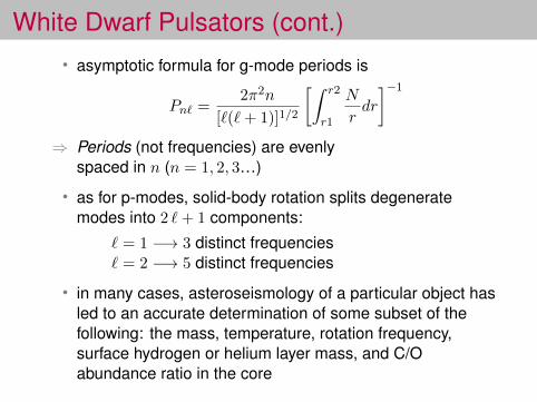
White Dwarf Pulsators (cont.)• asymptotic formula for g-mode periods is

Pn` =2π2n

[`(`+ 1)]1/2

[∫ r2

r1

N

rdr

]−1

⇒ Periods (not frequencies) are evenlyspaced in n (n = 1, 2, 3…)

• as for p-modes, solid-body rotation splits degeneratemodes into 2 `+ 1 components:

` = 1 −→ 3 distinct frequencies` = 2 −→ 5 distinct frequencies

• in many cases, asteroseismology of a particular object hasled to an accurate determination of some subset of thefollowing: the mass, temperature, rotation frequency,surface hydrogen or helium layer mass, and C/Oabundance ratio in the core

A DOV star: PG 1159-035

• 125 individual frequencies observed

• both ` = 1 and 2 modes observed

1991ApJ...378..326W

A DOV star: PG 1159-035 (cont.)

(Winget, D. E. et al. 1991, ApJ, 378, 326)

A DOV star: PG 1159-035 (cont.)

• proved beyond a shadow of a doubt that the modeswere g-modes corresponding to ` = 1, 2

• asteroseismologically derived parameters:

mass: 0.586± 0.003 Mrotation period: 1.38± 0.01 daysmagnetic field: . 6000 G

A DBV star: GD 358

10 consecutive ` = 1radial orders observed,with n=8–17(Winget et al. 1994, ApJ, 430, 839)

Power spectrum of the white dwarf GD 358

(Winget, D. E. et al. 1994, ApJ, 430, 839)

GD 358 (cont.)

• asteroseismologically derived parameters(Bradley & Winget 1994, Winget et al. 1994):

mass: 0.61± 0.03 MMHe: 2± 1× 10−6 M?

rotation period: ∼ 0.9–1.6 daysdifferential rotationimplied

luminosity: 0.05± 0.012Ldistance: 42± 3 pc

• measured parallax for GD 358 is 36± 4 pc⇒ agrees with asteroseismologically derived distance

However, looking more carefully reveals two classes ofasteroseismological fits…

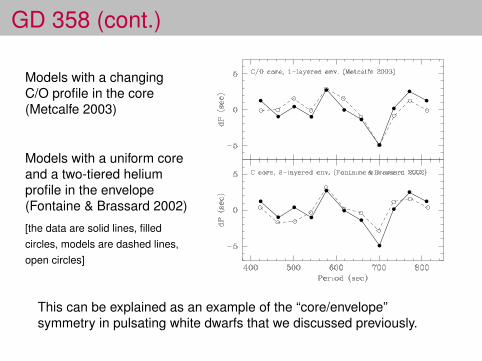
GD 358 (cont.)

Models with a changingC/O profile in the core(Metcalfe 2003)

Models with a uniform coreand a two-tiered heliumprofile in the envelope(Fontaine & Brassard 2002)

[the data are solid lines, filledcircles, models are dashed lines,open circles]

This can be explained as an example of the “core/envelope”symmetry in pulsating white dwarfs that we discussed previously.

GD 358 (cont.)

Genetic algorithm fitting techniques have recently beenapplied to white dwarf modeling (e.g., Metcalfe et al. 2000, ApJ,545, 974, Metcalfe, Montgomery, & Kawaler 2003):

• explore possibility of a 3He layer(Montgomery, Metcalfe, & Winget 2001, ApJ, 548, L53)

• constrain the 12C(α, γ)16O reaction rate(Metcalfe 2003)

• constrain the mass fraction of oxygenin the core: XO = 67–76 %(Metcalfe 2003; Metcalfe, Winget, & Charbonneau 2001, ApJ, 557, 1021)

• constrain neutrino emission rates, compare withStandard Model of particle physics(Winget et al. 2004, ApJ, 602, L109)

A DAV: BPM 37093

• White dwarfs predictedto crystallize as theycool (Abrikosov 1960,Kirzhnitz 1960, and Salpeter1961)

• crystallization delayscooling, adds ∼ 2 Gyrto Galactic disk agesbased on white dwarfcooling

• promise of deriving thecrystallized massfractionasteroseismologically

High mass⇒ crystallized(Montgomery & Winget 1999, ApJ, 526, 976)

BPM 37093 (cont.)

• BPM 37093 has been extensively observed with the WholeEarth Telescope (WET)

The effect of the crystallized core is to exclude the pulsationsfrom it (Montgomery & Winget 1999)

Preliminary results:BPM 37093 is ∼ 90 % crystallized by mass

(Metcalfe, Montgomery, & Kanaan 2004)

This would be the first “detection” of the crystallization processin a stellar interior.

As a cross-check of our approach, we will do a similar analysisfor a low-mass star which should be uncrystallized, and we willcheck if we do indeed find a best fit having 0% crystallization.

The Classical Cepheids

Yellow giants andsupergiants, radialpulsators, 1 or 2 modesexcited, periods ∼ 1 – 50days. This is

• great forPeriod-Luminosityrelationship (purelyempirical)

• bad for seismology –not enough modes!

(Sandage & Tammann 1968)

Subdwarf B/EC 14026 stars

• are Extreme Horizontal Branch (EHB) stars• recently predicted and then observed to pulsate

(Charpinet et al. 1996, ApJ, 471, L103)

• Teff ∼ 35, 000 K, log g ∼ 5.9

• driving is due to an opacity bump due to metals (inthis case, mainly Fe), as in the β Cephei stars

• gravitational settling and radiative levitation work toincrease the abundance of Fe in regions of theenvelope, enhancing the driving effect

Subdwarf B/EC 14026 stars

Typical lightcurves ofpulsating sdB stars(Charpinet et al. 2009, AIP Conf.

Proc. 1170, 585)

I. / , f. f. A * • A >

5.0

-5.0

^ V V \ A ^ V v ^ A W v V y V V ^ ^ . v ^

1 \ P-MODE PULSATORS

G-MODE PULSATORS: TIME AXIS COMPRESSED BY . FACTOR 3

-35.0 I ^ ^ ^ ^ ^ 0. 1000, 3000. 3000. 4000. 5000, 6000.

Time (seconds)

FIGURE 5. Typical lightcurves for pulsating sdB stars. The upper part (in blue) shows sections of lightcurves obtained for four rapid sdB pulsators (the V361 Hya stars) through PMT broadband photometry using a uniform sampling of 10 s. The lower part (in red) shows lightcurves obtained for four long period sdB pulsators (the VI093 Her stars) through CCD R-band photometry using a nearly constant sampling time of - 8 0 s .

many - if not all - of the sdB stars in that surface gravity, effective temperature range seem to develop these grav-ity mode oscillations. Let us mention that three stars are known to show both the g-mode and the j9-mode pulsa-tions. These hybrid pulsators lie near the red edge of the EC 14026 instability strip and the blue edge of the VI093 Her instability region. The two domains therefore over-lap.

of hot subdwarf stars and are responsible for the large chemical anomalies observed in their atmosphere, as re-called in previous sections.

If, overall, the agreement between models and obser-vations is excellent within this framework, difficulties still persist to explain in detail the observed nonadiabatic properties of hot pulsating subdwarfs. Improvements in this area are likely to come from a refined treatment of the physics involved in driving the oscillations, in partic-ular concerning microscopic diffusion and atomic data for opacity calculations. For instance, beyond iron itself which is the main contributor to the opacity bump, the role of other opaque elements such as nickel was empha-sized [29, 28]. Other physical mechanisms potentially competing with radiative levitation and gravitational set-tling, such as weak stellar winds and mixing processes, are also likely to influence the driving. For the interested reader, more can be found about the driving mechanism in hot subdwarf stars in the recent reviews by Charpinet et al. [6, 4] and Fontaine et al. [17].

ASTEROSEISMIC SOUNDING

The exploitation of stellar oscillations as probes of the structural properties of hot subwarf stars has seen im-portant progress in recent years, following the very first attempt made by Brassard et al. to analyse in detail a pulsating sdB star [2]. Thus far, the focus has mostly been on rapid EC 14026 pulsators that turn out to be par-ticularly well suited for detailed asteroseismic studies. Meanwhile, the g-mode sdB pulsators and the sdO pul-sators also possess a high potential for asteroseismology that has yet to be exploited. In the next sections, we recall the method developed for objective asteroseismic sound-ing of sdB stars and we summarize the most interesting recent achievements in this domain.

The driving mechanism

The physical processes responsible for the pulsations observed in hot subdwarf stars are well identified. For all three classes, a classical K-mechanism involving the iron-group elements (and mostly iron itself) through the so-called Z-bump structure occurring at a temper-ature of '-^ 200,000 K in the mean Rosseland opacity profile is responsible for the driving of the pulsations [14, 13, 20, 18]. For the mechanism to be efficient, how-ever, it is necessary to enhance well above solar propor-tions the amount of heavy metals, especially iron, present in that Z-bump region [13, 3]. This requirement can be naturally fulfilled through mechanisms involving selec-tive diffusive processes, such as radiative levitation, that are known to be efficient in the hot and stable envelope

Mandatory physics for the stellar models

The asteroseismic probing of sdB stars requires that sufficiently accurate stellar models are computed for a meaningful comparison of the theoretical pulsations pe-riods with those observed in the analyzed star. This re-quires that the most relevant pieces of physics must be implemented in the models. For sdB stars, the role of gravitational settling and radiative levitation has been shown to be central to understand many of the properties of these stars, from their atmospheric chemical composi-tion to the driving of pulsations. We want to emphasize that this fimdamental ingredient must also be considered for quantitative seismic analyses.

589

Downloaded 19 Apr 2013 to 128.83.129.41. This article is copyrighted as indicated in the abstract. Reuse of AIP content is subject to the terms at: http://proceedings.aip.org/about/rights_permissions

Subdwarf B/EC 14026 stars

(Charpinet et al. 2009, AIP Conf. Proc. 1170, 585)TABLE 2. Structural parameters from asteroseismology for a sample of 11 /i-mode sdB pulsators.

' " " " i„„i/f /i/f ^^ References Name Teff logg logMenv/M*

PG 1047+003 PG 0014+067 PG 1219+534 Feige 48 PG 1325+101 EC 20117^014 PG 0911+456 BAL 090100001 PG 1336-018 EC 09582-1137 PG 0048+091

33150±200 34130±370 33600 ±370 29580 ±370 35050 ±220 34800 ±2000 31940 ±220

28000 ±1200 32780 ±200 34806 ±233 33335±1700

5.800±0.006 5.775 ±0.009 5.807±0.006 5.437± 0.006 5.811±0.004 5.856±0.008 5.777 ±0.002 5.383 ±0.004 5.739± 0.002 5.788± 0.004 5.711±0.010

-3.72±0.11 -4.32 ±0.23 -4.25±0.15 -2.97 ±0.09 -4.18±0.10 -4.17±0.08 -4.69 ±0.07 -4.89±0.14 -4.54 ±0.07 -4.39±0.10 -4.92 ±0.20

0.490±0.014 0.477 ±0.024 0.457±0.012 0.460 ±0.008 0.499±0.011 0.540 ±0.040 0.390±0.010 0.432±0.015 0.459 ±0.005 0.485±0.011 0.447 ±0.027

[11] [10] [8] [9] [V] [43] [40] [46] [5] [38] in prep

should encourage fiirther efforts in that direction which can be twofold: 1) pursuing the analysis of more pulsat-ing sdB stars with current models and tools to clarify our global view of the internal properties of sdB stars, and 2) improving further the sounding power of asteroseis-mology applied to these stars. This second objective is becoming particularly relevant and can possibly take two directions.

proved opacity calculations (OPAL vs. OP), a treatment for possibly competing processes, such as stellar winds, meridional circulation, or thermohaline convection [45] that could modify the distribution of chemical species in-side the envelope. The strong constraints imposed by as-teroseismology should be extremely valuable to explore and better handle these phenomena in stellar models.

Improving the accuracy of the seismic fits

As recalled in a previous section, the current astero-seismic fits can reproduce the observed period spectrum of a star with a precision that is still significantly lower than the accuracy at which the periods can be measured. This fact points toward shortcomings in the physical de-scription implemented in stellar models currently used for asteroseismology. Despite these shortcomings, recent asteroseismic results have shown that such models are precise enough, however, to allow robust determinations of the main structural parameters with an already highly interesting level of accuracy. However, we expect that much more can be achieved by improving further the physical description of the star in the models with the ultimate goal of providing period fits that reach the pre-cision of the observations.

On this venture, current hints suggest to us that the pri-ority should be given to improve the treatment of diffu-sive processes and other competing mechanisms that can affect the chemical stratification in the stellar envelope, i.e., in regions where j9-modes are indeed sensitive to the structure of the star This is likely one of the main source of uncertainty that can possibly account for the limi-tations encountered with current asteroseismic models. Possible improvements could be a more complete treat-ment for the radiative levitation, including other species contributing significantly to the opacity (such as Ni), im-

Sounding deeper layers with the long period g-mode pulsators

Another interesting prospect is to exploit the long period g-mode pulsators (the VI093 Her stars) with the same asteroseismic methods. In B subdwarfs, acoustic waves are mostly confined in the outermost part of the star and do not permit to probe efficiently the deepest stellar regions (as shown, for example, by Figure 10, in the context of stellar rotation). Gravity modes, for their part, propagate much deeper in the star and are therefore more sensitive to the structure of these deep regions. Hence, the g-mode pulsators could potentially provide complementary information on the internal structure and dynamics of hot B subdwarf stars.

Asteroseismology of VI093 Her stars will hopefiilly benefit from the advent of space observations. The satel-lite COROT is programmed to observe a long period g-mode sdB pulsator in faU 2009 for a continuous, ^^ 20 day duration coverage. Such pulsators may also be found among the many variable stars discovered by this in-strument. In addition, programs to search and monitor long period sdB pulsators with the KEPLER satellite have been proposed. Space observations could provide the high quality seismic data needed for detailed stud-ies such as those performed to date for the EC 14026 stars. Such data have been difficult to obtain from ground based campaigns, so far

595

Downloaded 19 Apr 2013 to 128.83.129.41. This article is copyrighted as indicated in the abstract. Reuse of AIP content is subject to the terms at: http://proceedings.aip.org/about/rights_permissions

Other Pulsators

roAp stars: “rapidly oscillating Ap stars”• have magnetic fields and peculiar

chemical abundances• p-mode oscillators (∼ 5 minute periods)

with the pulsation axis inclined relative tothe magnetic axis

• driving mechanism not yet establisheddelta Scuti stars:

• ∼ 1.6–2.5M• p-mode oscillators, periods of hours• driven by the standard Kappa mechanism

Other Pulsators (cont.)

Gamma Doradus Stars:• g-mode oscillators, periods of one to

several days• probably driven by “convective driving”• long periods make it difficult to do

asteroseismologySolar-like stars:

• p-mode oscillators• stochastically driven (by convection zone)• periods of several minutes

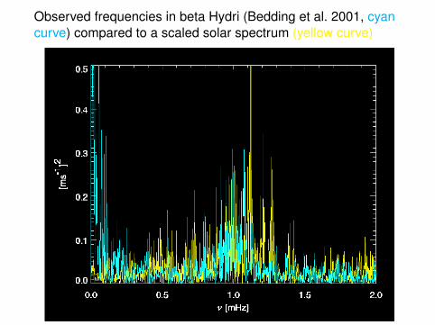
Observed frequencies in beta Hydri (Bedding et al. 2001, cyancurve) compared to a scaled solar spectrum (yellow curve)

Electronic copies of these notes (in living color) can befound at:

www.as.utexas.edu/˜ mikemon/pulsations.pdf

Good luck!