Level-1A to Level-1B Spacecraft data to Geolocation Data and Antenna Temperature

Level-1B to Level-2AAntenna Temperatures Converted to TOA Brightness Temperature

Level-2A to Level-2BSea-surface Salinity found from TOA TB plus Ancillary Data

Based on

Aquarius Science Pre-CDRLevel 1 and 2 Algorithms, Frank J. Wentz20-21 July, 2006

Algorithm Theoretical Basis DocumentAquarius Level-2 Radiometer Algorithm: Revision 1January 22 2008

Aquarius Data Processing

Aquarius

Sunsunlat,sunlonsundis

SolarReflection refllatrefllonreflinc

Gain AnglesDirect and Reflected Solartht_global_sun(2)phi_global_sun(2)

Boresight cellatcelloncelinccelazmcelpra

SolarBackscattersunincsunazmsunglt

GalaxyBig Bangglxlatglxlon(J2KM)

Moonmoonlat,moonlonmoondis

Earth Surface

Radiation Seen by Aquarius

Atmosphere

Level 1A DataEssentially Organized Version of Level 0

Data organized in orbital files Start near the South Pole where z-velocity=0.

Orbit contain 20% overlap on both ends Accommodate count averaging

Spacecraft Position in MJ2K Coordinates: [x, y, z, t] Coordinates have been verified with CONAE

Spacecraft Attitude [roll, pitch, yaw, t]

Radiometer Counts: Earth and Calibration

Thermistor Counts

Housekeeping Counts

Level-1A to Level-1B Processing

Geolocation

S/C subtrack latitude, longitude altitude, zang. For each horn observation every 1.44 sec:1. Geodetic latitude and east longitude2. Boresight incidence angle and azimuth angle 3. Sun incidence and azimuth angle (for backscattering computation)4. Polarization rotation angles relative to Earth5. Zenith and azimuth angles for sun and moon6. Zenith and azimuth angles for reflected ray (MJ2K coordinates)

Sun and MoonContamination

Approximate increase in TA due to (requires antenna pattern)1. Direct and Reflected Sun (assuming nominal flux)2. Reflected Moon

RFI DetectionFlags applied to radiometer countsEarth maps of number of occurrences stratified by horn number, pol, and asc/dsc

RadiometerCount Averaging

Earth Counts averaged 1.44 sec (one complete radiometer cycle)Calibration Counts averaged for longer time periods (TBD)

Convert Thermistor Counts to Temperature (K)

Level-1A DataAll time tagged, MJ2K coordinatesS/C Position, Velocity, AttitudeRadiometer CountsThermistor Counts

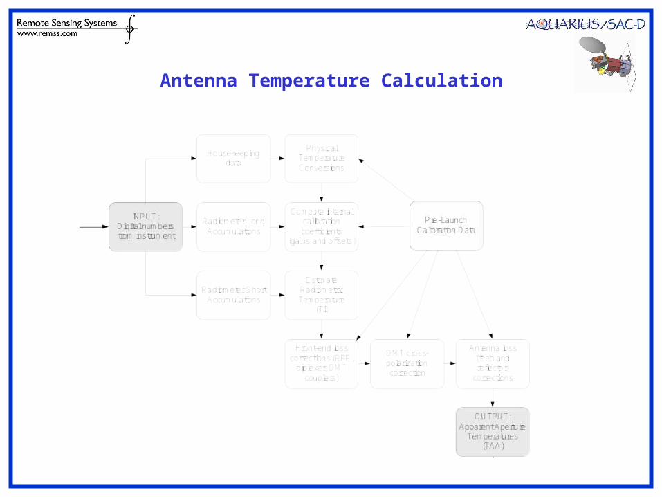
Compute Antenna Temperature

TAv, TAh, TAp, TAm (one value for each complete 1.44 s radiometer cycle)

Geolocation

Oblate Spheroid Earth Model: WGS-84 RE=6378.137D3, RP=6356.752D3

Sensor Point Geometry for 3 Horns Nadir Angle = [ 25.80o, 33.77o, 40.34o] Azimuth Angle= [ 9.76o, -15.33o, 6.50o] Rotation Matrix for Sensor/Spacecraft Misalignment

Vector formulation in MJ2K coordinates

Plenty of Heritage (SSM/I,TMI,AMSR, etc.)

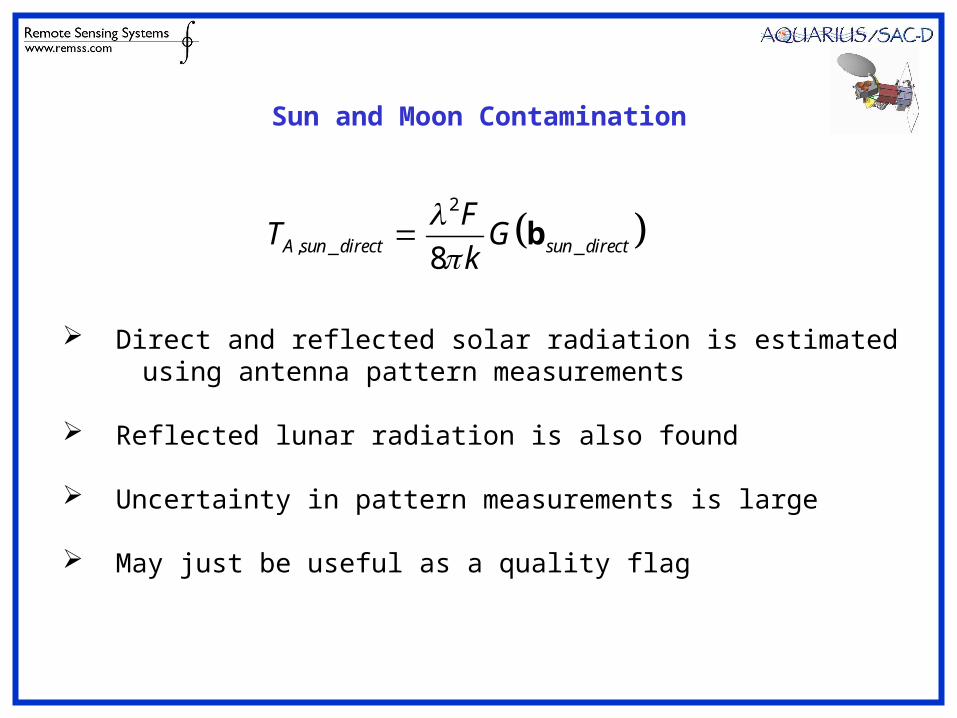
Sun and Moon Contamination

2

, _ _8A sun direct sun direct

FT G

k

b

Direct and reflected solar radiation is estimated using antenna pattern measurements Reflected lunar radiation is also found

Uncertainty in pattern measurements is large May just be useful as a quality flag

RFI Detection

Done before any averaging of Earth counts Statistical outlier analysis

Earth maps of persistent sources Suspected Earth counts are flagged and excluded from averaging

Count Averaging and Thermistor Temperatures

Earth counts are averaged for 1.44 sec (one complete radiometer cycle) Calibration counts are averaged over longer intervals

Thermistor counts are converted to physical temperatures using laboratory derived coefficients

Antenna Temperature Calculation

, ,

, ,

, 45 , 45

, ,

Amea V Amea H

Amea V Amea H

AAmea Amea

Amea left Amea right

T T

T T

T T

T T

T

,1 1

4 4i space

Earth Space

dA dA

A B BT G b R T G b T

1 0 0 0

0 cos2 sin 2 0

0 sin 2 cos2 0

0 0 0 1

f f

f f

R

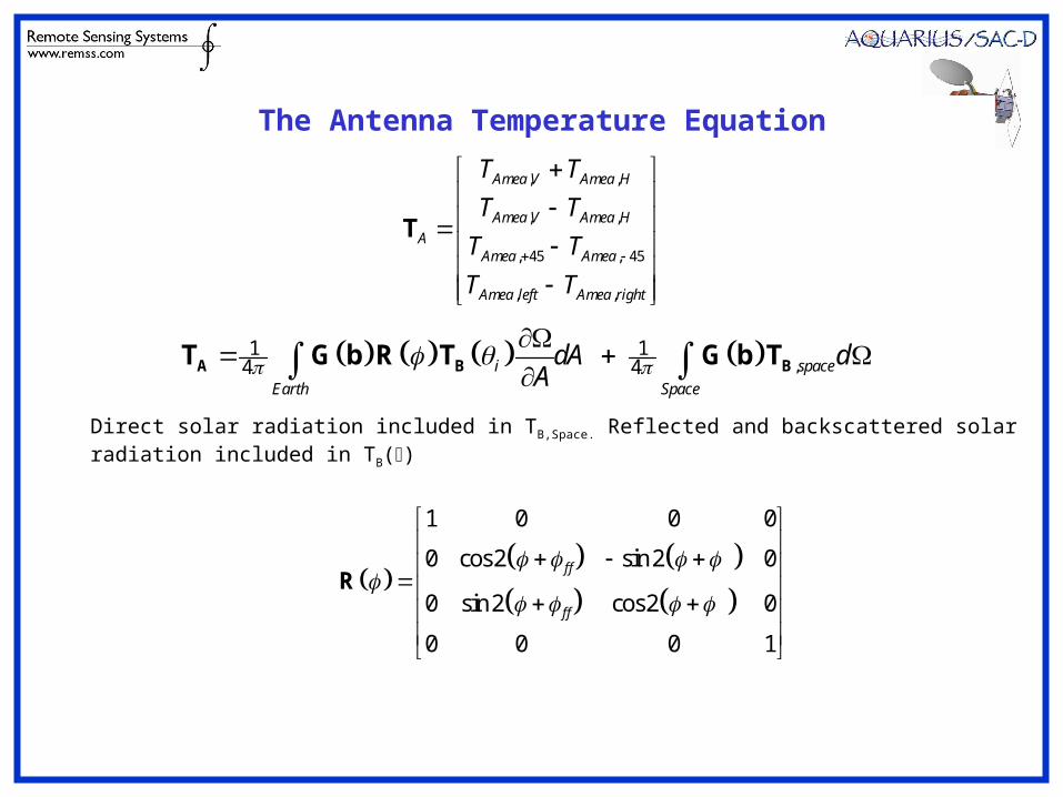
Direct solar radiation included in TB,Space. Reflected and backscattered solar radiation included in TB()

The Antenna Temperature Equation

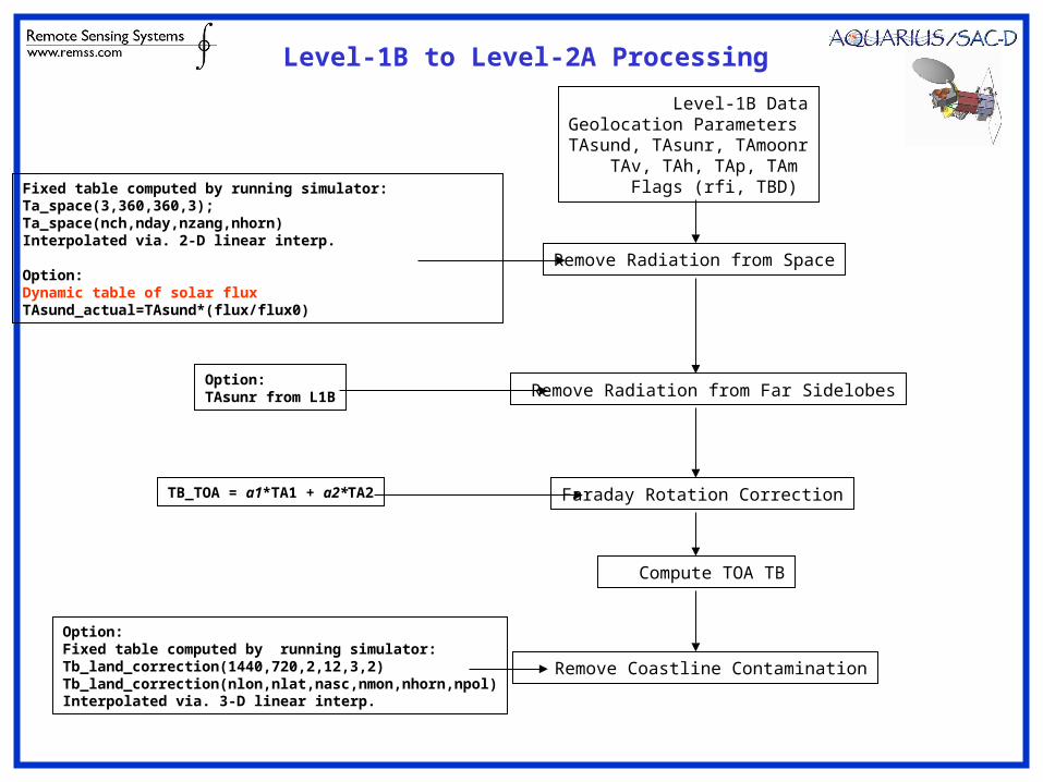
Level-1B to Level-2A Processing

Remove Radiation from Far Sidelobes

Option:Fixed table computed by running simulator:Tb_land_correction(1440,720,2,12,3,2)Tb_land_correction(nlon,nlat,nasc,nmon,nhorn,npol)Interpolated via. 3-D linear interp.

Fixed table computed by running simulator:Ta_space(3,360,360,3); Ta_space(nch,nday,nzang,nhorn)Interpolated via. 2-D linear interp.

Option:Dynamic table of solar fluxTAsund_actual=TAsund*(flux/flux0)

Faraday Rotation Correction

Compute TOA TB

Remove Radiation from Space

Level-1B DataGeolocation ParametersTAsund, TAsunr, TAmoonr TAv, TAh, TAp, TAm Flags (rfi, TBD)

Option:TAsunr from L1B

Remove Coastline Contamination

TB_TOA = a1*TA1 + a2*TA2

Removal of Radiation from Space

Cosmic background, TB=2.73 K

Galactic radiation (smoothed by antenna pattern)

Earth limb (very small, TA=0.006)

Pre-computed tables a function of day-of-year and orbit position

Direct solar radiation

(expected to be <0.05 K, optional, computed during Level-1)

Removal of Reflected Solar and Lunar Radiation

Reflected solar radiation

Expected to be <0.05 K, optional, computed during Level-1

Reflected lunar radiation

In mainlobe and may be correctable

Top of the Atmosphere (TOA) TB (slide 1)

Definition of TOA TB:A simple average (no weighting) of the upwelling brightness at the top of the atmosphereThe average is just over the 3-dB footprintThe incidence angle is constantAn effective incidence angle can be used in place of the boresight incidence angle.In other words: TOA TB is independent of antenna characteristics and is just a function of the environment and specified incidence angle.

Over the Open Ocean:Very detailed and elaborate simulations show:TB_TOA = a1*TA1 + a2*TA2to a 1-sigma accuracy of 0.04 K TA1 and TA2 and the first and second TA stokes measurements after removing space contributionand doing Faraday Rotation Correction.See The Estimation of TOA TB from Aquarius Observations, RSS Report 013006, January 30,

2006

Coefficients a1 and a2 determined before launch using scale-model antenna patterns.They may be revised after launch to remove any global, absolute difference between Aquarius TOA TB and TOA TB coming from the RTM.

Over Extended Land Areas:The expression:TB_TOA = a1*TA1 + a2*TA2still works very well, although a1 and a2 are slightly different

Areas Containing a Mixture of Land and Water:Very difficult to maintain accuracies required for salinity retrievalsPossibly one can extended salinity retrievals towards the coast by 100 km (?).

We propose using the simulator to produce correction tables.Tb_land_correction(1440,720,2,12,3,2) {0.5 GB} . 1440 by 720 is a 0.25 latitude, longitude map2 is ascending/descending orbit12 is months of year3 is horns2 is polarizations

Table can be redone at the end of the mission using more realistic L-band land temperatures.

Top of the Atmosphere (TOA) TB (slide 2)

Coastline Correction Table for Ascending Orbit Segments for 1st Stokes

Coastline Correction Map

Level-2A to Level-2B Processing

Remove Reflected and Scattered Radiation1. Galactic reflected2. Solar backscatter3. Moon reflected

NCEP Profiles of temperature, pressure, vaporInterpolated via. 3-D linear interp.

Compute atmospheric upwelling and downwellingradiation (TBup, TBdw) and transmittance t.

Salinity Retrieval Algorithm

Remove Radiation from the Atmosphere

Level-2A DataGeolocation Parameters TBtoav, TBtoah Flags (TBD)

NCEP 10-m windInterpolated via. 3-D linear interp.

Fixed table giving galactic maps with varying amounts of smoothingTB_gal(1440,720,21)TB_gal(nlon,nlat,nwind)Interpolated via. 3-D linear interp.

Options:solar backscatter=f(tht,thtsun,azm-azmsun,wind)TAmoonr from L1B.

!!! Salinity !!!

NCEP 10-m wind (TBR)NCEP SST (TBR)Interpolated via. 3-D linear interp.

Sea-Surface Emission

,,

BP toa BUBP sur P S BP

T TT E T T

,cos , ,BP BD B B gal P BP sunT T T T R T

Atmospheric parameters come from NCEP 6-hour fields Spatial averaging of galactic radiation is an important consideration Option for computing backscattered solar radiation

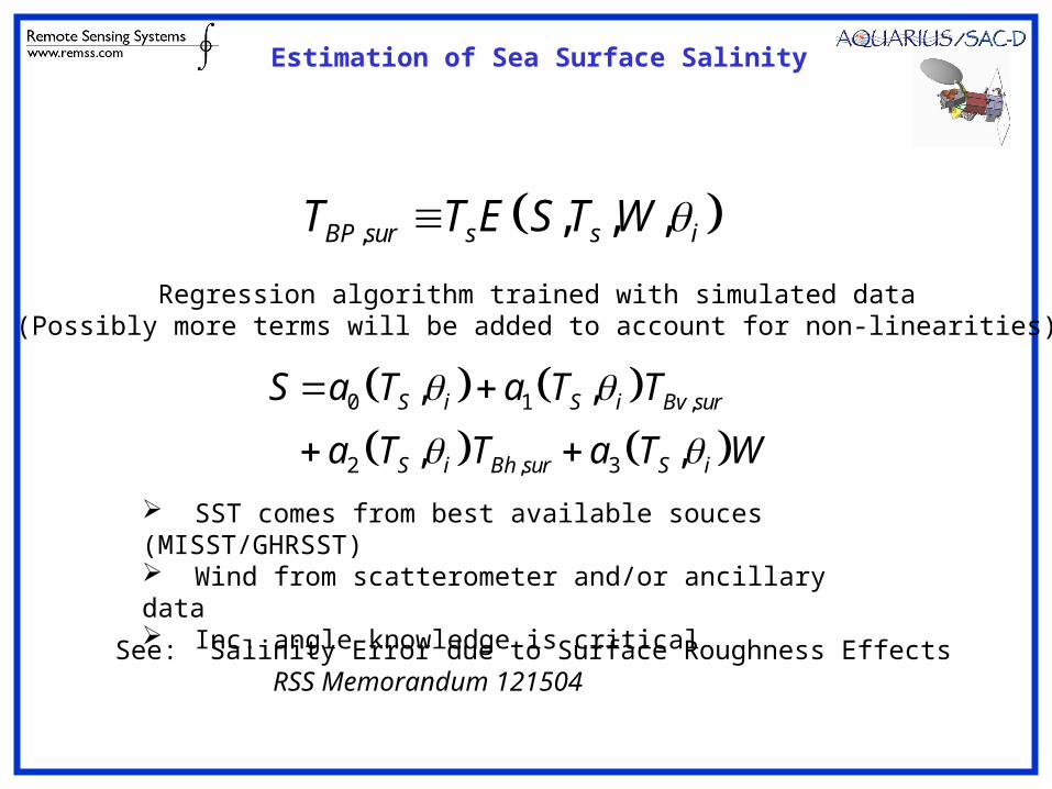
, , , ,BP sur s s iT T E S T W

0 1 ,

2 , 3

, ,

, ,

S i S i Bv sur

S i Bh sur S i

S a T a T T

a T T a T W

Regression algorithm trained with simulated data(Possibly more terms will be added to account for non-linearities)

SST comes from best available souces (MISST/GHRSST) Wind from scatterometer and/or ancillary data Inc. angle knowledge is critical

See: Salinity Error due to Surface Roughness Effects RSS Memorandum 121504

Estimation of Sea Surface Salinity

Earth SceneOcean: Salinity, SST, Wind fieldsLand: Soil moisture, vegetation type, LSTIce: Ice type and temperatureAtmosphere (including limb): NCEP profiles

TA IntegrationFull 4-Stokes Integration over Earth and Space

SunYear 2000 actual values Easily scalable

Cosmic Background 2.7 K

GalaxyTo be implemented

Faraday Rotation Actual TEC valuesEarth Magnetic Field

Orbiting AntennaCONAE Orbit ParametersRoll/Pitch/Yaw now includedAquarius Scale Model patterns

Radiometer Piepmeier Forward Model for TA to counts

TB TB

TB

TB

TBrotated

TA

Radiometer Counts

Orbiting Thermal ModelSimple harmonic of orbit position

Thermistor Response Func. Linear with temperature

Temperatures

Thermistor Counts

Orbit Position

End-to-End Aquarius On-Orbit Simulator: Part 1

End-to-End Aquarius On-Orbit Simulator: Part 2

Radiometer Counts Thermistor Counts

Pre-FormatterFormat in Group, Block, and Sub-Block Structure

Telemetry FormatterFormat in Group, Block, and Sub-Block Structure

Scatterometer Data Platform Data

Simulated Downlink Telemetry

Level-0 to Level-1A Processing

Level-1A to Level-1B Processing

Level-1B to Level-2 Processing

Level-2 to Level-3 Processing

Antenna Temperature

TOA Brightness TemperatureSwath Salinity, SST, wind, etc

Time-Averaged Salinity Fields

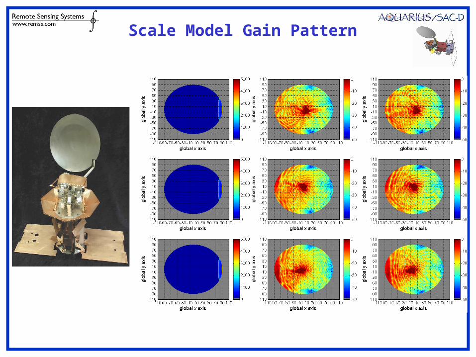
Scale Model Gain Pattern

• Includes

– surface temperature and moisture from NCEP (simultaneous)

– Surface type (bare, ice, grass, crop, tree (tropical, deciduous, conifer)) from EUROCLIMAP monthly/annual climatology

– Soil roughness effect

– Vegetation effect

– L-band dielectric model of Dobson et al. 1985

Land Emissivity Model

• Simulates, based on ATBD (Piepmeier/Pellerano/Wilson/Yueh 2005) – radiometer (Ta counts)

– Ta retrieval (counts Ta)

• Used minimum 2 calibration looks for v-/h-pol and 4 calibration looks for 3 rd Stokes

• Fully used correlated noise diodes

• Accuracy is better than 0.01K

Testing TA Counts TA

Components of Aquarius On-orbit Simulator

1. Complete integration of the 4-Stokes parameters over the complete 4steradians

2. Direct and reflected solar radiation for year 2000

3. Cosmic and galactic spillover contribution (galactic TBI)

4. Earth Limb Contribution

5. Faraday rotation in the ionosphere

6. Full slant-path integration through NCEP atmospheres

7. Surface emissivity from NCEP wind fields, Reynolds SST fields, & ECCO salinity model.

8. Intensive numerics with integration error < 0.01 K

Error Modeling for Aquarius On-orbit Simulator

1. Year 2000 (maximum of last solar cycle) used for ionosphere electron density

2. Worst case Faraday rotation (Julian day 303 in 2003)

3. NEDT for 6-sec average = 0.08 K

3. Incidence angle knowledge error is 0.03 deg std. dev. error added to incidence angle

4. SST knowledge error is 0.3 C

5. Wind speed knowledge error is 0.5 m/s (also 1.0 m/s)

6. Six-hour variability added to atmospheric model

7. No correction for solar radiation (included in simulation but not retrieval)

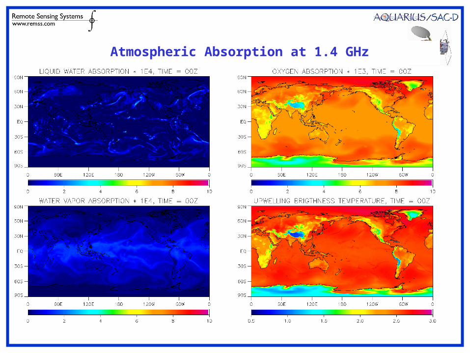
Atmospheric Absorption at 1.4 GHz

Global Results for Salinity Retrievals (7-days)

Reference

Retrieval

s

Salinity Retrieval Performance (7days)

Mean

Std. Dev.

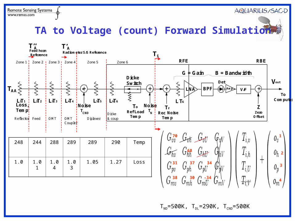
LNA Det

Amp V/F V out

+

T r Rec Noise

Temp

Z Zero

Offset

T o Ref Load

Temp

G = Gain Dicke Switch

+

L T 6 To

Computer

BPF

B = Bandwidth

Noise T

N

T i

+

Noise T

CND

+

L 6 T 6 L 5 T 5 L 4 T 4 L 3 T 3 L 2 T 2 L 1 T 1 Loss, Temp

Zone 6 Zone 5 Zone 4 Zone 3 Zone 2 Zone 1

T ’ A Radiometer S/S Reference

T AA

RFE RBE

Diplexer OMT Coupler

OMT Feed Reflector Dicke & coup

T ’’ A Feed horn Reference

31 37 34

70 1

38 30 -34

682

3

4

248 244 288 289 289 290 Temp

1.0 1.01 1.04 1.03 1.05 1.27 Loss

TND=500K, TDL=290K, TCND=500K

TA to Voltage (count) Forward Simulation

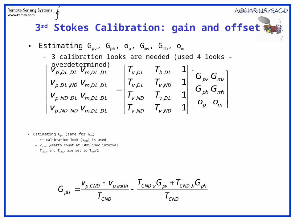
3rd Stokes Calibration: gain and offset

, , , , , ,

, , , , , ,

, , , , , ,

, , , , , ,

1

1

1

1

p DL DL m DL DL v DL h DLpv mv

p DL ND m DL DL v DL v NDph mh

p ND DL m DL DL v ND v DLp m

p ND ND m DL DL v ND v ND

v v T TG G

v v T TG G

v v T To o

v v T T

• Estimating Gpv, Gph, op, Gmv, Gmh, om

– 3 calibration looks are needed (used 4 looks - overdetermined)

• Estimating GpU (same for GmU)

– 4th calibration look (vCND) is used

– vp,earth=earth count at 10milisec interval

– TCND,v and TCND,h are set to TCND/2

, , , ,p CND p earth CND v pv CND h phpU

CND CND

v v T G T GG

T T

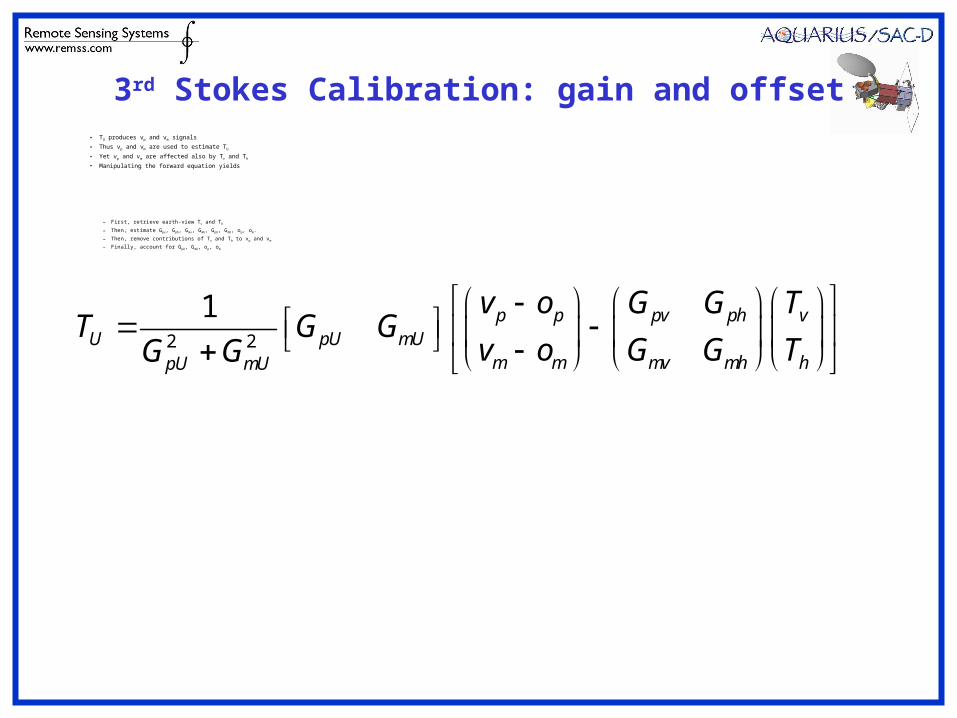
3rd Stokes Calibration: gain and offset• TU produces vp and vm signals

• Thus vp and vm are used to estimate TU

• Yet vp and vm are affected also by Tv and Th

• Manipulating the forward equation yields

– First, retrieve earth-view Tv and Th

– Then, estimate Gpv, Gph, Gmv, Gmh, GpU, GmU, op, om.

– Then, remove contributions of Tv and Th to vp and vm

– Finally, account for GpU, GmU, op, om

2 2

1 p p pv ph vU pU mU

m m mv mh hpU mU

v o G G TT G G

v o G G TG G