Embed Size (px)
Citation preview
Research report manuscript No.(will be inserted by the editor)
Level Bundle Methods for Constrained Convex Optimization with
Various Oracles
Wim van Ackooij · Welington de Oliveira
Received: May 23, 2013
Abstract We propose restricted memory level bundle methods for minimizing constrained convexnonsmooth optimization problems whose objective and constraint functions are known throughoracles (black-boxes) that might provide inexact information. Our approach is general and cov-ers many instances of inexact oracles, such as upper, lower and on-demand oracles. We showthat the proposed level bundle methods are convergent as long as the memory is restricted toat least four well chosen linearizations: two linearizations for the objective function, and twolinearizations for the constraints. The proposed methods are particularly suitable for both jointchance-constrained problems and two-stage stochastic programs with risk measure constraints.The approach is assessed on realistic joint constrained energy problems, arising when dealing withrobust cascaded-reservoir management.
Keywords Nonsmooth Optimization · Stochastic Optimization · Level Bundle Method · ChanceConstrained Programming
Mathematics Subject Classification (2010) MSC 49M37 · MSC 65K05 · MSC 90C15
1 Introduction
In this work we consider problems of the type
minx
f0(x) s.t. x ∈ X ⊂ Rn and fj(x) 6 0 for j = 1, ...,m , (1)
Wim van AckooijEDF R&D. OSIRIS1, avenue du General de Gaulle, 92141 Clamart Cedex, FranceTel.: +33-(0)1-47-655831Fax: +33-(0)1-47-653037
Wim van AckooijEcole Centrale ParisGrande Voie des Vignes, F-92295, Chatenay-Malabry, FranceE-mail: [email protected]
Welington de OliveiraInstituto Nacional de Matematica Pura e Aplicada - IMPARua Dona Castorina 110, 22460-320, Rio de Janeiro, BrazilE-mail: [email protected]
2 Wim van Ackooij, Welington de Oliveira
where fj : Rn → R, j = 0, ...,m are convex functions and X 6= ∅ a polyhedral bounded set in R
n.We will make the assumption that some (or all) functions fj are hard to evaluate. We thereforeassume that the mappings fj , j = 1, ...,m can be inexactly evaluated by some oracle (or black-box) providing approximate values and subgradients, hereafter denoted by oracle information. Theprecision of the oracle information might be unknown, but it is assumed bounded.
Many optimization problems arising from real-life applications cast into the above framework. Forsome problems, as in large-scale stochastic optimization or in combinatorial optimization, comput-ing exact information from the oracle is too expensive, or even out-of-reach, whereas computingsome inexact information is still possible. For these type of problems, optimization algorithmsbased only on exact oracle information can be impracticable, unless some simplifications on theproblems are made.
Applications in which a decision maker has to make a decision hedging risks often lead to optimiza-tion problems with nonlinear convex constraints that are difficult to deal with. For instance, if suchconstraints (fj , with j = 1, . . . ,m) are setup as joint chance constraints (see Example 2 below).Evaluating the functions for a given point involves computing numerically a multidimensionalintegral. This is a difficult task when uncertainty variables are high-dimensional (say dimension100), see [4]. A second difficulty is obtaining an efficient estimate of a subgradient. This can bedone in many cases of interest, but equally involves imprecisions (see [2] for a special case and[33–35] for very general results).
The last few years have seen the occurrence of a new generation of bundle methods, capable to han-dle inexact oracle information. For unconstrained (or polyhedral constrained) convex nonsmoothoptimization problems we refer to [12] and [16] for general approaches, [18] for a combinatorialcontext, and [9], [8], [22] and [20] for a stochastic optimization framework. For an encompassingapproach we refer to the recent work [21].
For constrained convex optimization problems like (1) more sophisticated methods need to comeinto play. We refer to [9] and [7] for level bundle methods capable to deal with asymptoticallyexact oracle information. Such oracle information is assumed to underestimate the exact value ofthe functions, i.e., the oracle is of the Lower type. Since [9] and [7] are based on the pioneeringwork [19], they are not readily implementable because they might require unbounded storage,i.e. all the linearizations built along iterations must be kept. The recent work [4] overcomes thisdrawback and furthermore allows for Upper Oracles, i.e., oracles that provide inexact informationwhich might overestimate the exact values of the functions. In contrast to [9] and [7] that employlevel bundle methods, the work [4] applies a proximal bundle method, see also [13]. These worksdefine different improvement functions (see (8) below) to measure the improvement of each iteratetowards a solution of the problem. Level bundle methods have at disposal lower bounds (self-built)to define improvement functions, in contrast to proximal bundle that must find other alternativesto the (not at hand) lower bounds. We refer to [4], [30] and [14] for some improvement functionalternatives.
Due to the improvement function definition, level bundle methods are likely to be more preferablethan proximal bundle methods to handle (nonlinear) constrained convex optimization problems.For this reason we follow some features of the restricted memory level bundle method proposedin [15] and extend [7] to handle Upper Oracles and to keep the storage information bounded; thisis what we call restricted memory. Moreover, we extend [4] by considering Upper Oracles withon-demand accuracy (see the formal definition in § 4.2), and like [7] we prove convergence forLower Oracles with on-demand accuracy without assuming a Slater point.
This work is organized as follows: Section 2 presents two important examples of optimizationproblems that cast into the problem formulation (1), with difficult to evaluate objective and/orconstraint functions. In Section 3 we propose our algorithm and prove its convergence for exactoracle information. The convergence analysis therein is the key for proving convergence of thealgorithm when inexact oracle information come into play. Section 4 deals with inexact oracleinformation. We consider Upper, Lower, and on-demand oracles, depending on the assumptions
Level Bundle Methods for Constrained Convex Optimization with Various Oracles 3
made. In Section 5 we provide numerical experiments on realistic joint chance constrained energyproblems, arising when dealing with robust cascaded-reservoir management. These are problemsfrom Electricite de France – EdF. We compare the proposed approaches with some algorithmsconsidered in [4]. The paper ends with concluding comments and remarks.
To easy notation, in what follows we consider a short formulation to problem (1). Without lossof generality we may assume that m = 1 in (1) by defining the (nonsmooth and convex) functionc : R
n → R
c(x) := maxj=1,...,m
fj(x) ,
and call f0 just f . With this notation, the problem we are interested in solving is
fmin := minx∈X⊂Rn
f(x) s.t. c(x) 6 0 , (2)
which is assumed to have a solution; therefore, its optimal value fmin is finite.
2 Some examples coming from stochastic optimization
We now provide two examples coming from stochastic optimization that can be cast into the abovescheme, wherein f and/or c are difficult to evaluate.
Example 1 (Risk-averse two-stage stochastic programming) Let Z ⊂ Rn be a bounded polyhedral
set. Let also Ξ ⊂ Rd be a finite set containing elements (scenarios) ξi, i = 1, . . . , N ; and suppose
that ϕ : Z → R is a convex function. A two-stage stochastic problem with mean-CV@R aversionmodel and finitely many scenario can be written as
min ϕ(z) +∑N
i=1 piQ(z, ξi)
s.t. t + 1β
∑Ni=1 pi[Q(z, ξi)− t]+ 6 ρ
z ∈ Z, t ∈ R ,
(3)
where 1 > β > 0 and ρ > 0 are given parameters, pi > 0 is the probability associate to the scenarioξi, [·]+ denotes the positive part of a real number, and Q : Z × Ξ → R is a convex function on Zdefined for instance by the linear problem
Q(z, ξ) :=
min 〈q, y〉s.t. W (ξ)y + T (ξ)z = h(ξ)
y ∈ Rn2+ .
The components q,W, T and h are assumed to be mesurable mappings with appropriate dimensionsand well defined in Ξ.
Problem (3) is a risk-averse two-stage stochastic programming problem. The nonlinear and difficult
to evaluate constraint t + 1β
∑Ni=1 pi[Q(z, ξi) − t]+ 6 ρ is the so called conditional value-at-risk
(CV@Rβ) with confidence level β; see [27], [28], [7].
By bounding the variable t, writing x = (z, t) ∈ X ⊂ Y × R, and by taking
f(x) = f(z, t) = ϕ(z) +
N∑
i=1
piQ(z, ξi) and c(x) = c(z, t) = t +1
β
N∑
i=1
pi[Q(z, ξi)− t]+ − ρ
problem (3) corresponds to (2). Notice that computing the value of the functions f(x) and c(x)for each given point x ∈ X amounts to solving N linear problems Q(x, ξi), i = 1, . . . , N . Afterhaving solved those linear problems, subgradients for f and c are easily at hand; see [31] for moredetails. Therefore, for large N (say N > 10000) the functions f and c are hard to evaluate, andby making use of inexact oracle information (e.g., solving inexactly or just skipping some linearproblems) problem (3) can be numerically tractable even for a large N . ut
4 Wim van Ackooij, Welington de Oliveira
This kind of problems are taken into account in [7], by considering Lower Oracles with on-demandaccuracy (see § 4.4 for the formal definition). Besides the conditional value-at-risk approach of two-stage stochastic programs, [7] considers more risk-aversion concepts such as stochastic dominancemeasure, proposed in [6]. In all cases, no Upper Oracles are studied.
Example 2 (Chance-constrained programming) Given a probability level p, the (differentiable) op-timization problem
min 〈q, x〉s.t. P[Ax + a 6 ξ 6 Ax + b] > p
x ∈ X(4)
has a feasible set that is convex for d-dimensional random variables ξ with log-concave probabilitydistribution (but in many other settings too). In this formulation, A is a fixed matrix and a, b arefixed vectors with appropriate dimensions. Evaluating the constraint and computing a gradientwith high precision is possible but potentially very costly, especially when the dimension d is large(say d ≥ 100).
By a classical result ([23, Thm. 4.2.4]), not only the feasible set induced by the joint chanceconstraint in (4) is convex but also the function
log(p)− log(P[Ax + a 6 ξ 6 Ax + b]) . (5)
Therefore, problem (4) corresponds to (2) by taking
f(x) = 〈q, x〉 and c(x) = log(p)− log(P[Ax + a 6 ξ 6 Ax + b]) .
The oracle for the function c(x) employs multidimensional numerical integration and quasi-MonteCarlo techniques for which the error sign is unknown (but a bound is computable). ut
Take x ∈ X . Since the inexact oracle information can overestimate the exact value c(x) (UpperOracle), the constrained level bundle methods proposed in [7] is not suitable.
In what follows we propose a new algorithm to deal with (in-)exact oracle information.
3 Level Bundle Method for Exact Oracles
In this section we assume that both functions f and c in (2) can be exactly evaluated by an oraclethat provides for each xk ∈ X :
{
f -oracle information: f(xk) and gkf ∈ ∂f(xk)
c-oracle information: c(xk) and gkc ∈ ∂c(xk) .
(6)
With such information from the oracle, we consider the approximate linearizations
fk(x) := f(xk) + 〈gkf , x− xk〉
ck(x) := c(xk) + 〈gkc , x− xk〉 .
At iteration k, two polyhedral cutting-plane models are available:
fk(x) := maxj∈Jk
f
f j(x) with Jkf ⊂ {1, 2, . . . , k} (7a)
ck(x) := maxj∈Jk
c
cj(x) with Jkc ⊂ {1, 2, . . . , k} . (7b)
It follows from convexity that
fk(x) 6 f(x) and ck(x) 6 c(x) for all k and for all x ∈ X .
Level Bundle Methods for Constrained Convex Optimization with Various Oracles 5
Given a lower bound fklow for fmin, we define the so called improvement function at iteration k by
hk(x) := max{f(x)− fklow, c(x)} . (8)
As already mentioned, the above definition of improvement function is not possible for proximalbundle methods, since the lower bounds fk
low are not available. Some alternatives for fklow must be
taken instead.
We have the following important result.
Lemma 1 Consider the improvement function hk given in (8). Then, hk(x) > 0 for all x ∈ Xand for each iteration k. If there exists a sequence {xk
rec} ⊂ X such that limk hk(xkrec) = 0, then
any cluster point of the sequence {xkrec} is a solution to problem (2). In particular, if hk(xk
rec) = 0for some k then xk
rec is a solution to problem (2).
Proof Let x ∈ X and k be arbitrary. If c(x) 6 0, then f(x) > fklow by definition of fk
low; on theother hand, if f(x) < fk
low then x cannot be feasible, i.e., c(x) > 0. It thus follows trivially thathk(x) > 0 for all x ∈ X , as x and k were taken arbitrarily.
Assume that a sequence {xkrec} ⊂ X such that limk hk(xk
rec) = 0 is given. It follows from (8) thathk(xk
rec) ≥ f(xkrec) − fk
low > f(xkrec) − fmin. We can thus conclude (i) 0 > limk(f(xk
rec) − fklow) >
limk(f(xkrec)− fmin) and similarly (ii) 0 > limk c(xk
rec).
Let x be a cluster point of the sequence {xkrec} ⊂ X . Then x ∈ X and by (ii) c(x) 6 0. Therefore,
since x is feasible, by (i) we have that 0 > limk(f(xkrec)− fmin) = f(x)− fmin > 0. Hence, x is a
solution to problem (2).
In particular, if hk(xkrec) = 0 for some k then 0 > f(xk
rec)− fmin and 0 > c(xkrec), showing that xk
rec
is a solution to problem (2).
That having been said, we will provide an algorithm that generates a sequence of iterates {xk} ⊂ X ,a subsequence of recorded iterates {xk
rec} ⊂ {xk}, a nondecreasing sequence of lower bounds {fk
low}for fmin, and a sequence of levels fk
lev ≥ fklow such that
fklow ↑ fmin, fk
lev → fmin and hk(xkrec)→ 0 .
In order to do so, at iteration k we obtain a new iterate xk+1 by projecting a given stability centerxk ∈ X (not necessary feasible for c) onto the level set
Xk := {x ∈ X : fk(x) 6 fk
lev , ck(x) 6 0} (9)
whenever it is nonempty. Obtaining xk+1 amounts to solving the following quadratic problem(QP)
xk+1 := arg minx∈Xk
1
2|x− xk|2 , or just xk+1 := PXk(xk) for short. (10)
Whenever Xk is empty, the current level fk
lev and lower bound fklow require updating.
The following proposition provides us with properties of the minimizer xk+1. We will use thenotation NX for the normal cone of convex analysis of a set X .
Proposition 1 The point xk+1 solves (10) if and only if xk+1 ∈ X , fk(xk+1) 6 fklev, ck(xk+1) 6
0, and there exist vectors gkf ∈ ∂fk(xk+1), gk
c ∈ ∂ck(xk+1), sk ∈ NX (xk+1) and stepsizes µkf , µk
c >
0, such that
xk+1 = xk − (µkf gk
f + µkc gc + sk) , µk
f (fk(xk+1)− fklev) = 0 and µk
c ck(xk+1) = 0 . (11)
In addition, the aggregate linearizations
faf (k)(·) := fk(xk+1) + 〈gkf , · − xk+1〉 satisfies faf (k)(x) 6 fk(x) 6 f(x) for all x ∈ X (12a)
6 Wim van Ackooij, Welington de Oliveira
cac(k)(·) := ck(xk+1) + 〈gkc , · − xk+1〉 satisfies cac(k)(x) 6 ck(x) 6 c(x) for all x ∈ X . (12b)
Moreover,PXk(xk) = PXa(k)(xk) (13)
holds, where Xa(k) is the aggregate level set defined as X
a(k) := {x ∈ X : faf (k)(x) 6 fklev, cac(k)(x) 6
0}.
Proof Let iX be the indicator function of the polyhedral set X , i.e., iX (x) = 0 if x ∈ X andiX (x) =∞ otherwise. Remembering that the set X 6= ∅ is polyhedral and by [26, p.215] ∂iX (x) =NX (x) for x ∈ X , the first claim results from the KKT conditions for problem (10) rewritten as
minx∈Rn12 |x− xk|2 + iX (x)
s.t. fk(x) 6 fklev
ck(x) 6 0 .
The subgradient inequality gives (12).
We now proceed to show (13). Notice that PXa(k)(xk) is the solution to the following QP:
minx∈Rn12 |x− xk|2 + iX (x)
s.t. faf (k)(x) 6 fklev
cac(k)(x) 6 0 .(14)
Moreover, x solves the above problem if, and only if, there exist ρ, λ > 0 and s ∈ NX (x) such that
x = xk − (ρgkf + λgc + s) , ρ(faf (k)(x)− fk
lev) = 0 and λcac(k)(x) = 0 .
Notice that by taking ρ = µkf , λ = µk
c and s = sk above, the resulting x = xk+1 satisfiesthe optimality conditions for problem (14). Since (14) has a unique solution, we conclude thatxk+1 = PXa(k)(xk), as stated.
The interest of the aggregate level set is that Xa(k) condenses all the past information relevant for
defining xk+1. This property is crucial for the bundle compression mechanism to be put in place.Namely, the property makes it possible to change the feasible set X
k in (10), possibly with manyconstraints, by any smaller set containing X
a(k). In this manner, the size of the bundles Jkf and
Jkc in (7) can be kept controlled, thus making (10) easier to solve; see comment (g) below.
We are now in position to give the algorithm with full details. In the algorithm we will keeptrack of special iterations called “critical iterations” that allow us to either progress significantlyin the quest of solving (2) or improve our currently proven lower bound for fmin in (2). Criticaliterations are counted with l. All iterations are counted with k. Iterations between the changeof the critical iteration counter from l to l + 1 are said to belong to the l-th cycle. We willmoreover denote with k(l) the critical iteration at the start of the l-th cycle and hence Kl ={k(l), k(l) + 1, . . . , k(l + 1) − 1} is the index set gathering the iterations in the l-th cycle. Therecorded sequence {xk
rec} is constructed by defining x0rec equal to the first iterate x0 and
xkrec :=
xk−1rec if
[
minj∈Jkf ∩Jk
chk(xj) > hk−1(xk−1
rec ) and k > 1
or {Jkf ∩ Jk
c } = ∅,arg minj∈Jk
f ∩Jkc
hk(xj) otherwise.(15)
Algorithm 1 We assume given an oracle computing f/c values as in (6) for any x ∈ X .
Step 0 (Input and Initialization) Choose a parameter γ ∈ (0, 1) and a stopping toleranceδTol > 0. Given x0 ∈ X and a lower bound f0
low 6 fmin, set x0 ← x0. Call the oracle to obtain(f(x0), g0
f ) and (c(x0), g0c ) and set l← 0, k ← 0, k(l)← 0, J0
f ← {0} and J0c ← {0}.
Step 1 (Best Current Minimizer) Update the recorded sequence xkrec according to (15).

Level Bundle Methods for Constrained Convex Optimization with Various Oracles 7
Step 2 (Stopping Test) Perform the stopping test hk(xkrec) 6 δTol. If satisfied return xk
rec andf(xk
rec).
Step 3 (Descent Test) In this optional Step we test if hk(xkrec) ≤ (1 − γ)hk(l)(x
k(l)rec ). If so we
declare a critical iteration and we set l← l + 1, k(l)← k and choose xk ∈ {xj : j ∈ Jkf ∩ Jk
c }.
Step 4 (Level Updating) Set fklev ← fk
low + γhk(xkrec) and update the feasible set X
k given in(9).
Step 5 (Quadratic Program) Try to solve the quadratic program (10). If no feasible solutionis found then declare a critical iteration, set l ← l + 1, k(l) ← k, fk
low ← fklev and choose
xk ∈ {xj : j ∈ Jkf ∩ Jk
c }. Return to Step 1. If problem (10) is solved then move to Step 6.
Step 6 (Oracle) Call the oracle to obtain (f(xk+1), gk+1f ) and (c(xk+1), gk+1
c ).
Set fk+1low ← fk
low and xk+1 ← xk.
Step 7 (Bundle Management) Manage the bundle freely as long as Jk+1f ⊃ {k +1, af(k)} and
Jk+1c ⊃ {k + 1, ac(k)} remain true at each bundle compression.
Step 8 (Loop) Set k = k + 1 and go to Step 1.
We can provide the following remarks concerning Algorithm 1:
(a) The sequence {hk(xkrec)} is monotonically decreasing by (8) and (15).
(b) Let Kl be the index set belonging to the l-th cycle, it then follows that both the stabilitycenter xk and lower bound fk
low are fixed for all k ∈ Kl. As a consequence,
for each fixed l ≥ 0, the sequence {f jlev}j∈Kl is nonincreasing. (16)
This property is essential for Lemma 3.It may happen by Step 3 and 5 that Kl is an empty set. In the convergence analysis given belowwe simply assume that Kl is nonempty for each l. This strategy eases the calculations withoutloosing generality.
(c) If the level set Xk is empty, this means that fk
lev < fk(x) for all x ∈ {z ∈ X : ck(z) 6 0}. Sinceck(·) 6 c(·), it follows that {z ∈ X : c(z) 6 0} ⊆ {z ∈ X : ck(z) 6 0} and thus, fk
lev < fk(x)for all x ∈ {z ∈ X : c(z) 6 0}. As fk(·) 6 f(·) we conclude that fk
lev is a lower bound for theoptimal value fmin. Therefore, the updating rule fk
low ← fklev at Step 4 gives a valid lower bound
for fmin.
(d) Whenever the level set is empty at Step 5, the lower bound fklow is increased by at least an
amount of γhk(xkrec) > 0 and the cycle-counter l is incremented by one. Moreover fk
low 6 fmin forall k > 0. Assume that δTol = 0. If there is an infinite loop between Steps 5 and 1, one concludes
that fk(l+1)low > f
k(l)low because the stopping test in Step 2 fails. Since fmin <∞ is an upper bound
on this sequence, we must therefore have that hk(xkrec)→ 0. Hence, if δTol > 0 there cannot be
an infinite loop between Steps 5 and 1.
(e) In order to avoid excessively short cycles, we can solve the following linear problem to updatefklow at Step 5:
fklow = min
x∈Xfk(x) s.t. ck(x) 6 0 . (17)
As fklev > fk
low, then Xk will be nonempty.
(f) If problem (17) is solved at each iteration at Step 3, then the level set Xk is nonempty. However,
this procedure might not ensure (16) and thus Lemma 3 below holds only if there is no bundlecompression along each cycle Kl, i.e., Jk+1
f = Jkf ∪ {k + 1} and Jk+1
c = Jkc ∪ {k + 1} for all
k ∈ Kl. For more details see [19, p. 121] or [20, Lemma 3.5].
(g) In fact, the aggregate linearizations (12) do not need to be included in the bundle at eachiteration but only when the bundle is compressed. This provides a versatile framework for dealingwith bundle compression and avoid encumbering memory.Considering that the bundle is full (we have saved more elements than some a priori bound), aquite practical rule would consist of keeping only the active linearization index sets, i.e., delete
8 Wim van Ackooij, Welington de Oliveira
inactive ones:
Jkf := {j ∈ Jk
f : f j(xk+1) = fklev} and Jk
c := {j ∈ Jkc : cj(xk+1) = 0} .
If the bundle is still considered full, we can replace any two indices i, j ∈ Jkf by af(k) (respectively
i, j ∈ Jkc by ac(k)) until the Bundle is sufficiently cleaned up. Then we update as follows:
Jk+1f = Jk
f ∪ {k + 1} and Jk+1c = Jk
c ∪ {k + 1} .
(h) After having solved problem (10), each constraint f j(xk+1) 6 fklev with j ∈ Jk
f (respec.
ci(xk+1) 6 0 with i ∈ Jkc ) has a Lagrange multiplier αj
f > 0 (respec. αic > 0). Furthermore, it
follows from the cutting-plane definition that gjf ∈ ∂f(xk+1) for all j ∈ Jk
f such that αjf > 0
(respec. gic ∈ ∂c(xk+1) for all i ∈ Jk
c such that αic > 0). In this manner, by taking µk
f =∑
j∈Jkf
αjf
and gkf = 1
µkf
∑
j∈Jkf
αjfgj
f (respec. µkc =
∑
j∈Jkc
αjc and gk
c = 1µk
c
∑
j∈Jkc
αjcg
jc) the aggregate lin-
earizations (12) can be easily obtained. If µkf = 0, then all constraints f j(xk+1) 6 fk
lev are
inactive (the inequality holds strictly) and all the bundle Jkf information is useless. Then the
aggregate linearization fa(k) is also inactive. The equivalent conclusion holds if µkc = 0. Lemma 2
below ensures that µkc = µk
f = 0 cannot happen, otherwise we would have xk+1 = xk.
Steps 6 and 7 in Algorithm 1 are optional in a way. We can consider two important alternativeswhich will be particularly useful when either the f or the c oracle is costly.
A variant of Algorithm 1 for costly c-oracles
The following strategy is useful if, for instance, the constraint oracle information (c(xk+1), gk+1c )
is more difficult to obtain than the information (f(xk+1), gk+1f ). This is the case of Example 2.
Avoiding to compute the c-oracle information if xk+1 does not give a significant decrease.
Step 6(f) (Oracle) Set fk+1low ← fk
low, xk+1 ← xk and call the oracle to obtain (f(xk+1), gk+1f ).
If f(xk+1) > fklev +(1−γ)hk(xk
rec) go to Step 7(f). Otherwise, before going to Step 7(f) compute(c(xk+1), gk+1
c ).
Step 7(f) (Bundle Management) Manage the bundle freely as long as:– (If both f(xk+1) and c(xk+1) were computed at Step 6(f))Jk+1
f ⊃ {k + 1, af(k)} and Jk+1c ⊃ {k + 1, ac(k)} hold true at each bundle compression.
– (If c(xk+1) was not computed at Step 6(f))Jk+1
f ⊃ {k + 1, af(k)} and Jk+1c ⊃ {ac(k)} hold true at each bundle compression.
We emphasize that the test f(xk+1) > fklev + (1− γ)hk(xk
rec) implies that the c-oracle informationis computed only if f(xk+1) < max{f(xk
rec), fklow + c(xk
rec)}, i.e., when f(xk+1) provides decreasewith respect to at least one of the two thresholds f(xk
rec) or fklow + c(xk
rec).
A variant of Algorithm 1 for costly f-oracles
For the case in which (f(xk+1), gk+1f ) is more difficult to compute than (c(xk+1), gk+1
c ) Algorithm 1may consider the following strategy.
Avoiding to compute the f-oracle information if xk+1 is far from feasibility.
Step 6(c) (Oracle) Set fk+1low ← fk
low, xk+1 ← xk and call the oracle to obtain (c(xk+1), gk+1c ).
If c(xk+1) > (1 − γ)hk(xkrec) go to Step 7(c). Otherwise, before going to Step 7(c) compute
(f(xk+1), gk+1f ).
Step 7(c) (Bundle Management) Manage the bundle freely as long as:– (If both f(xk+1) and c(xk+1) were computed at Step 6(c))Jk+1
f ⊃ {k + 1, af(k)} and Jk+1c ⊃ {k + 1, ac(k)} remain true at each bundle compression.
– (If f(xk+1) was not computed at Step 6(c))Jk+1
c ⊃ {k + 1, ac(k)} and Jk+1f ⊃ {af(k)} remain true at each bundle compression.
According to the above two strategies, we consider the following three versions for Algorithm 1:

Level Bundle Methods for Constrained Convex Optimization with Various Oracles 9
Algorithm 1(fc) Algorithm 1 as it is stated;
Algorithm 1(f) Algorithm 1 with Steps 6 and 7 replaced by Steps 6(f) and 7(f);
Algorithm 1(c) Algorithm 1 with Steps 6 and 7 replaced by Steps 6(c) and 7(c).
Remark 1 Notice that the index set Jkf ∩Jk
c can be empty for versions (f) and (c) of Algorithm 1.If it is the case, the choice of the next stability center xk at Steps 3 and 5 is not well defined. Wemay proceed as follows according to Steps 6(f) and 6(c):
– At Steps 3 and 5 of Algorithm 1(f), choose xk ∈ {xj : j ∈ Jkf ∩ Jk
c } if Jkf ∩ Jk
c 6= ∅.
Otherwise, xk ∈ {xj : j ∈ Jkf and f(xj) > f j−1
lev + (1− γ)hj−1(xj−1rec )}.
– At Steps 3 and 5 of Algorithm 1(c), choose xk ∈ {xj : j ∈ Jkf ∩ Jk
c } if Jkf ∩ Jk
c 6= ∅.Otherwise, xk ∈ {xj : j ∈ Jk
c and c(xj) > (1− γ)hj−1(xj−1rec )}.
Here comes an interesting feature of Algorithm 1: differently from the constrained level bundlemethods [19], [15], [9], [7] and version (fc), the versions (f) and (c) of Algorithm 1 do not needto include the two linearizations fk+1 and ck+1 into the bundle at each iteration k. As shown inTheorem 2 below, even considering less oracle information, versions (f) and (c) provide the samecomplexity result than version (fc).
Convergence analysis of the above three versions ((fc), (f) and (c)) of Algorithm 1 is given in thefollowing subsection.
3.1 Convergence analysis
Throughout this section we suppose the feasible set X in (2) is compact with diameter D, anddenote by Λf > 0 (respectively Λc) a Lipschitz constant for the objective function (respectivelyconstraint) over the set X . Therefore, Λ := max{Λf , Λc} is a Lipschitz constant for hk, definedin (8). In what follows, both constants D and Λ can be unknown, since they are not used by thealgorithm but only to give upper bounds for the length of cycles Kl.
In the following lemma, we extend the result given in [15, Lemma 3.1] to our setting.
Lemma 2 Let l ≥ 0 be arbitrary, Λ = max{Λf , Λc} and γ ∈ (0, 1) be given. At iteration k of anyversion (fc), (f) or (c) of Algorithm 1, the following estimates hold:
|xk+1 − xk| >(1− γ)
Λhk(xk
rec) if k > k(l)
|xk+1 − xk| >(1− γ)
Λhk(xk
rec) if k = k(l) .
Proof Let us split this proof in three cases: we consider Algorithm 1(fc) first, then Algorithm 1(f)and finally Algorithm 1(c). We now study the first case.
Let k be arbitrary and j ∈ Jkf ∩ Jk
c be given. By (9) combined with (10), we get
f(xj) + 〈gjf , x
k+1 − xj〉 6 fklev
c(xj) + 〈gjc , x
k+1 − xj〉 6 0 .
By applying the Cauchy-Schwarz inequality we thus derive
f(xj)− fklev 6 |gj
f ||xk+1 − xj | 6 Λf |xk+1 − xj |
c(xj) 6 |gjc ||x
k+1 − xj | 6 Λc|xk+1 − xj | .
10 Wim van Ackooij, Welington de Oliveira
Since Λ = max{Λf , Λc}, fklev = fk
low + γhk(xkrec) and hk(xk
rec) > 0, we conclude that
Λ|xk+1 − xj | > max{f(xj)− fklow − γhk(xk
rec), c(xj)}
> max{f(xj)− fklow − γhk(xk
rec), c(xj)− γhk(xkrec)}
= −γhk(xkrec) + max{f(xj)− fk
low, c(xj)}
= −γhk(xkrec) + hk(xj) (18)
> (1− γ)hk(xkrec) .
Assuming that k > k(l), then the Oracle and Bundle Management steps assure that k ∈ Jkf ∩ Jk
c .Hence the estimate (18) with j = k provides the result. When k = k(l), the stability center xk ischosen among the bundle members. Hence, there exists a j ∈ Jk
f ∩ Jkc such that xj = xk and (18)
allows us to conclude this proof for the first case.
For versions 1(f) and 1(c) of Algorithm, if k ∈ Jkf ∩ Jk
c or j ∈ Jkf ∩ Jk
c with xj = xk nothingmore needs to be shown. Consider Algorithm 1(f) and j ∈ Jk
f but j /∈ Jkc together with f(xj) −
f j−1lev > (1 − γ)hj−1(xj−1
rec ) which holds for j = k and j s.t. xj = xk. As f j−1lev > fk
lev by (16) andhj−1(xj−1
rec ) > hk(xkrec) by (15) and comment (a), it follows that
f(xj)− fklev > (1− γ)hk(xk
rec) .
Since xk+1 is feasible for (10), then f(xj) + 〈gjf , x
k+1 − xj〉 6 fklev. All together we conclude that
Λ|xk+1 − xj | > 〈gjf , x
j − xk+1〉 > f(xj)− fklev > (1− γ)hk(xk
rec),
which was to be shown.
Consider Algorithm 1(c) and j ∈ Jkc but j /∈ Jk
f such that c(xj) > (1− γ)hj−1(xj−1rec ), which holds
for j = k and j s.t. xj = xk. In this case we obtain c(xj) > (1− γ)hj−1(xj−1rec ) > (1− γ)hk(xk
rec),where the last inequality follows from (15). Since xk+1 is feasible for (10), then 0 > c(xj) +〈gj
c , xk+1 − xj〉. It follows from Cauchy-Schwarz inequality that
Λ|xk+1 − xj | > 〈gjc , x
j − xk+1〉 > c(xj) > (1− γ)hk(xkrec) ,
which concludes the proof.
Lemma 2 shows that consecutive iterates are different. The following result implies that each cycleKl is finite.
Lemma 3 Let l ≥ 0 be arbitrary, D be the diameter of the feasible set X and Λ = max{Λf , Λc}.Assume that at each bundle compression in the versions (fc), (f) and (c) of Algorithm 1 we includethe aggregate indices in the bundle during the l-th cycle. Then, for all three versions (fc), (f) and(c) of Algorithm 1, any iteration k in the l-th cycle (i.e., k ∈ Kl) with hk(xk
rec) > δTol may differno more from k(l) than the following bound:
k − k(l) + 1 6
(
ΛD
(1− γ)hk(xkrec)
)2
Proof Let k ∈ Kl be such that k > k(l). It follows from (10) that xk = PXk−1(xk−1); thus
〈xk−1 − xk, x− xk〉 6 0 for all x ∈ Xk−1. (19)
If no bundle compression took place between step k−1 and step k, it holds that fk(x) > fk−1(x),ck(x) > ck−1(x) for all x ∈ R
n. Since fklev ≤ fk−1
lev by (16), it follows that Xk ⊆ X
k−1. Since kbelongs to the l-th cycle, X
k is nonempty and xk+1 ∈ Xk. This fact combined with xk−1 = xk
and (19) allows us to deduce that⟨
xk − xk, xk+1 − xk⟩
≤ 0. When bundle compression tookplace between steps k − 1 and k, the aggregate indices belong to the bundle for each of the three
Level Bundle Methods for Constrained Convex Optimization with Various Oracles 11
considered versions, i.e., af(k − 1) ∈ Jkf and ac(k − 1) ∈ Jk
c for Algorithms 1(fc), 1(f) and 1(c).This implies fk(x) > faf (k−1)(x), ck(x) > cac(k−1)(x) for all x ∈ R
n. It follows from (13) thatxk = PXa(k−1)(xk−1) and thus,
〈xk−1 − xk, x− xk〉 6 0 for all x ∈ Xa(k−1) . (20)
Since fklev ≤ fk−1
lev by (16), it follows that Xk ⊂ X
a(k−1). Similarly as before we can use (20) toobtain
⟨
xk − xk, xk+1 − xk⟩
6 0 for each of the versions (fc), (f) and (c). Therefore, by developingsquares in the identity |xk+1 − xk|2 = |xk+1 − xk + (xk − xk)|2 we have that
|xk+1 − xk|2 > |xk − xk|2 + |xk+1 − xk|2 .
As hk(xrec) > δTol for all k ∈ Kl, Algorithm 1 does not stop and xk = xk(l). A recursive applicationof the above inequality implies
|xk+1 − xk|2 > |xk − xk|2 + |xk+1 − xk|2
= |xk − xk−1|2 + |xk+1 − xk|2
> |xk−1 − xk−1|2 + |xk − xk−1|2 + |xk+1 − xk|2
...
> |xk(l)+1 − xk(l)|2 +
k∑
j=k(l)+1
|xj+1 − xj |2.
Since X is compact with diameter D and both xk+1 and xk are in X , then D > |xk+1 − xk|.Together with Lemma 2, this yields the bounds
D2>
(
(1− γ)
Λhk(xk
rec)
)2
+
k∑
j=k(l)+1
(
(1− γ)
Λhk(xk
rec)
)2
=
(
(1− γ)
Λhk(xk
rec)
)2
(k − k(`) + 1) ,
and result follows as k was arbitrary.
If the stopping test tolerance is set to zero, we now show that any cluster point of the recordedsequence of points generated by any version of Algorithm 1 solves problem (2).
Theorem 1 Consider any version (fc), (f) or (c) of Algorithm 1. Suppose that δTol = 0 and thatthe algorithm does not terminate. Then limk hk(xk
rec) = 0 and any cluster point of the sequence{xk
rec} is a solution to problem (2).
Proof If any version of Algorithm 1 stops at iteration k with hk(xkrec) = 0, by Lemma 1 xk
rec is anoptimal solution to problem (2).
If the algorithms do not stop, then by Lemma 3 (each cycle Kl is finite) we conclude that l→∞.Let W (respec. L) be an index set gathering counters l updated at Step 3 (respec. Step 5) of (anyversion of) Algorithm 1.
Let li be the i-th index in W = {l1, l2 . . . , }. Therefore, the inequality hk(li)(xk(li)rec ) 6 (1 −
λ)hk(li−1)(xk(li−1)rec ) holds even if there exists some l ∈ L such that li−1 < l < li. A recursive
application of the previous inequality gives us
0 6 hk(li)(xk(li)rec ) 6 (1− λ)hk(li−1)(xk(li−1)
rec ) 6 . . . 6 (1− γ)ihk(0)(xk(0)rec ) .
As both function f and c are finite valued, ifW has infinitely many indices then limi hk(li)(xk(li)rec ) =
0. Moreover, limk hk(xkrec) = 0 by monotonicity; see (15).
Let us now suppose that W is finite. As l→∞, then the index set L has infinitely many indices.
As fk(l+1)low is increased at Step 5 of the algorithm by an amount of γhk(xk
rec) > 0 for each l ∈ L,we obtain that limk hk(xk
rec) = 0 (otherwise we would have fklow ↑ ∞, which contradicts fk
low 6
fmin <∞).
We have shown in both cases (W finite or infinite) that limk hk(xkrec) = 0. Hence, the stated result
follows from Lemma 1.
12 Wim van Ackooij, Welington de Oliveira
3.2 Complexity results
We now provide an upper bound for the maximum number of iterations performed by versions(fc), (f) and (c) of Algorithm 1 in order to reach a given tolerance δTol > 0. To do so, we considerall the versions of Algorithm 1 without the optional Step 3.
Theorem 2 Let D be the diameter of the feasible set X and Λ = max{Λf , Λc}. Let −∞ < f1low 6
fmin be given in all versions (fc), (f) and (c) of Algorithm 1 and let the Step 3 be deactivated.Assume that at each bundle compression the aggregate indices are included in the bundle. Then,to reach an optimality measure hk(xk
rec) smaller than δTol > 0 Algorithms 1(fc), 1(f) and 1(c)perform at most
(
1 +fmin − f1
low
γδTol
)(
ΛD
(1− γ)δTol
)2
iterations.
Proof Consider any arbitrary but fixed version of Algorithm 1. Notice that every time that Xk = ∅,
the lower bound fklow for the optimal value fmin is increased by an amount of γhk(xk
rec) (> γδTol).Since f1
low is finite, the maximum number of cycles lmx times the stepsize γδTol is less thanfmin − f1
low, i.e.,
lmx6
fmin − f1low
γδTol.
It follows from Lemma 3 that each cycle Kl has at most(
ΛD(1−γ)δTol
)2
iterations, where we have
used that hk(xkrec) > δTol since the algorithm did not stop at iteration k. Let K(δTol) := {1, 2, . . . , }
be the index set for which hk(xkrec) > δTol. We have thus shown that K(δTol) is finite and if kδTol
is its maximal element, then:
kδTol 6
(
1 +fmin − f1
low
γδTol
) (
ΛD
(1− γ)δTol
)2
,
as was to be shown.
Notice that the better is the initial lower bound f1low for the optimal value fmin, the lower is
the upper bound for the maximum number of iterations performed by any considered version ofAlgorithm 1. If a lower bound f1
low is not available, we might obtain an initial lower bound bysolving a linear program, as follows.
Corollary 1 In the setting of Theorem 2, suppose that the initial lower bound f1low is defined as
f1low = min f1(x) s.t. c1(x) 6 0 , x ∈ X .
Then, fmin − f1low 6 2ΛfD and to reach an optimality measure hk(xk
rec) smaller than δTol > 0Algorithms 1(fc), 1(f) and 1(c) perform at most
(
1 +2ΛfD
γδTol
)(
ΛD
(1− γ)δTol
)2
iterations.
Proof We have that fmin = f(xmin) 6 f(x1) + ΛfD. Let x be a solution to the above linearprogram. Then f1
low = f1(x) = f(x1)+ 〈g1f , x−x1〉 > f(x1)−ΛfD by Cauchy-Schwarz inequality.
The result follows by combining the preceding inequalities and invoking Theorem 2.
So far we have considered only exact oracle information. In the next section we deal with inexact-ness from the oracle.
Level Bundle Methods for Constrained Convex Optimization with Various Oracles 13
4 Level Bundle Method for Inexact Oracles
In this section we assume that both functions f and c in (2) are inexactly evaluated. In whatfollows we will assume that the oracle provides us for each x ∈ X with
f -oracle information
[
fx = f(x)− ηxf and
gfx ∈ R
n such that f(·) > fx + 〈gfx, · − x〉 − εx
f
c-oracle information
[
cx = c(x)− ηxc and
gcx ∈ R
n such that c(·) > cx + 〈gcx, · − x〉 − εx
c
(21)
for some unknown ηxf , ηx
c , εxf , εx
c ∈ R.
By substituting fx = f(x)− ηxf in the second inequality and evaluating at x we derive that ηx
f >
−εxf . Similarly we observe that ηx
c > −εxc . Therefore, gf
x ∈ ∂(ηxf +εx
f )f(x) and gcx ∈ ∂(ηx
c +εxc )c(x).
Throughout this section we will make the assumption that the error on each of these estimates isbounded, i.e., there exist constants ηf , ηc, εf , εc > 0 such that
|ηxf | 6 ηf , εx
f 6 εf , |ηxc | 6 ηc, εx
c 6 εc for all x ∈ X . (22)
With such information from the oracle, we consider the approximate linearizations
fk(x) := fxk + 〈gfk, x− xk〉 and ck(x) := cxk + 〈gc
k, x− xk〉 (23)
to set up the cutting-plane models in (7), which gives
fk(x) 6 f(x) + εf and ck(x) 6 c(x) + εc for all k and all x ∈ X . (24)
Since both functions f and c in (2) are convex, the feasible set X is compact, and the oracle errorsin (21) are bounded (it follows from (21) and (22) that −ηf 6 εx
f 6 εf and −ηc 6 εxc 6 εc), [13,
Prop.XI.4.1.2] ensures that there exists a constant Λ such that
Λ > max{|gfx|, |gc
x|}; for all x ∈ X . (25)
Given a (approximate) lower bound fklow for the optimal value fmin in (2), we define the inexact
improvement function byhk
i (x) = max{fx − fklow, cx} . (26)
Due to inaccuracy from the oracle, we can have hki (x) < 0.
Lemma 4 Consider the improvement function hki given in (26). If there exists a sequence {xk
rec} ⊂X such that limk hk
i (xkrec) 6 0, then any cluster point of the sequence {xk
rec} is a η-solution toproblem (2), with a possibly unknown error η := max{ηf + εf , ηc}.
Proof By (24) the lower bound updating at Step 5.2 ensures that fklow 6 fmin + εf .
If limk hki (xk
rec) 6 0, it follows by (26), the definition of η and oracle assumptions that
(i) 0 > limk
(fxkrec− fk
low) > limk
(f(xkrec)− ηf − fk
low) > limk
(f(xkrec)− ηf − fmin − εf) ,
(ii) 0 > limk
cxkrec
> limk
c(xkrec)− ηc .
Let x be a cluster point of the sequence {xkrec} ⊂ X . Then x ∈ X and we conclude by (i) and (ii)
that f(x) 6 fmin + ηf + εf and c(x) 6 ηc, i.e, x is a η-solution to problem (2).
We now show that Lemma 2 still holds when all the three versions of Algorithm 1 are applied withthe inexact improvement function hi of (26).
14 Wim van Ackooij, Welington de Oliveira
Lemma 5 Let l ≥ 0 be arbitrary, Λ be the bound in (25) and γ ∈ (0, 1) be given. At iteration k ofall versions (fc), (f) and (c) of Algorithm 1 applied to improvement function hi of (26), assumethat hk
i (xkrec) ≥ 0 holds. Then the following estimates are true:
|xk+1 − xk| >(1− γ)
Λhk
i (xkrec) if k > k(l)
|xk+1 − xk| >(1− γ)
Λhk
i (xkrec) if k = k(l) .
Proof In the following we focus on the version (fc), i.e., Algorithm 1(fc). The proofs for theremaining two versions can be obtained in a similar manner to the proof of Lemma 2.
Let k be arbitrary and j ∈ Jkf ∩ Jk
c be given. By (9) combined with (10) and assumptions (21),we get
fxj + 〈gfj , xk+1 − xj〉 6 fk
lev
cxj + 〈gcj , xk+1 − xj〉 6 0 .
By applying the Cauchy-Schwarz inequality we thus derive
fxj − fklev 6 |gf
j ||xk+1 − xj | 6 Λ|xk+1 − xj |
cxj 6 |gcj ||xk+1 − xj | 6 Λ|xk+1 − xj | .
Since fklev = fk
low + γhki (xk
rec) and hki (xk
rec) > 0 by assumption, we conclude that
Λ|xk+1 − xj | > max{fxj − fklow − γhk
i (xkrec), cxj}
> max{fxj − fklow − γhk
i (xkrec), cxj − γhk
i (xkrec)}
= −γhki (xk
rec) + max{fxj − fklow, cxj}
= −γhki (xk
rec) + hki (xj) (27)
> (1− γ)hki (xk
rec) .
Assuming that k > k(l), then the Oracle and Bundle Management steps assure that k ∈ Jkf ∩ Jk
c .Hence the estimate (18) with j = k provides the result. When k = k(l), the stability center xk ischosen among the bundle members. Hence, there exists a j ∈ Jk
f ∩ Jkc such that xj = xk and (27)
allows us to conclude this proof.
Similarly Lemma 3 can be derived by a slight change of conditions, as shown below.
Lemma 6 Let l ≥ 0 be arbitrary, D be the diameter of the feasible set X and Λ be the bound of(25). Consider the versions (fc), (f) and (c) of Algorithm 1, with improvement function hi givenin (26). Assume that at each bundle compression in all versions (fc), (f) and (c) of Algorithm1 we include the aggregate indices in the bundle during the l-th cycle. Then, any iteration k inthe l-th cycle (i.e., k ∈ Kl) may differ no more from k(l) than the following bound, provided thathj
i (xjrec) > δTol > 0 for all j ≤ k:
k − k(l) + 1 6
(
ΛD
(1− γ)hki (xk
rec)
)2
The proof of the above lemma is identical to the proof of Lemma 3.
In what follows we make a distinction on the possible oracle types (21). We start by consideringthe most general case: Upper Oracles.
Level Bundle Methods for Constrained Convex Optimization with Various Oracles 15
4.1 Inexact constrained level methods for upper oracles
An Upper Oracle is an oracle of type (21) wherein εf > 0 and/or εc > 0 in (22) might occur. This inparticular implies that ηx
f , ηxc can be negative too and that the f - (c-) values can be overestimated.
Since in this case (24) holds, we can no longer keep Step 5 of Algorithm 1 as we can no longerassure that fk
lev remains a lower bound for fmin. We thus suggest to change Step 5 as follows:
Step 5 (Upper) Try to solve the quadratic program (10). If no feasible solution is found:
Step 5.1 solve the linear problem
valLP := min∑
j∈Jkc
sj s.t. x ∈ X , cj(x)− sj 6 0 ∀ j ∈ Jkc . (28)
If valLP > 0, stop (the problem is εc-infeasible); otherwise,
Step 5.2 Declare a critical iteration, set l← l + 1, k(l)← k, fklow ← fk
lev and choose xk ∈ {xj :j ∈ Jk
f ∩ Jkc }. Return to Step 1.
If problem (10) is solved then move to Step 6.
We thus obtain the following convergence result.
Theorem 3 Consider any version (fc), (f) or (c) of Algorithm 1, wherein Step 5 is replaced byStep 5 (Upper) applied with an Upper Oracle (21) and improvement function hk
i given in (26).Suppose that δTol = 0 and that the algorithm does not terminate. Then limk hk
i (xkrec) 6 0 and any
cluster point of the sequence {xkrec} is a η-solution to problem (2), with η := max{ηf + εf , ηc}.
Proof Given the assumptions Lemma 6 holds. Proceed similarly as in the proof of Theorem 1to show that limk hk
i (xk) 6 0, where fmin should be substituted by f + ηf . Here f is defined asf := minx :c(x)≤−εc f(x). It is easily observed that fk
low is a proven lower bound for f + ηf and
hence indeed hki (xk
rec) must tend to zero. We can now use Lemma 4 to conclude.
Since the bounds given in Lemmas 3 and 6 are the same, we conclude that the complexity resultof Theorem 2 also holds for inexact oracle satisfying (21). Up to our knowledge, general inexactoracles satisfying (21) have not been considered for (nonlinear) constrained level bundle methods.In [9] and [7] only Lower Oracles (see § 4.3 below) are considered. The work [4] deals with UpperOracles by applying a proximal bundle method.
Theorem 3 assumes that the algorithm does not terminate. This is not the case when problem (2)is detected to be εc-infeasible, i.e., {x ∈ X : ck(x) 6 0} = ∅ in Step 5.1. In the following sectionwe deal with εc-infeasibility by making additional assumptions on problem (2) and oracle (21).
4.2 Inexact constrained level methods for upper oracles with on-demand accuracy
In this subsection we additionally assume that:
– problem (2) has a Slater point, i.e., there exists a point xs ∈ X such that c(xs) < 0;
– demanding more accuracy on the c-information from (21) is possible (the upper bound εc in (22)might be demanded to decrease).
From (21) one directly derives that ck(x) 6 c(x) + εc for all x ∈ X . This shows that upper oracleshave nonetheless
{x ∈ Rn : c(x) 6 −εc} ⊆
{
x ∈ Rn ck(x) 6 0
}
. (29)
Now if the optimal value valLP of the LP (28) is strictly positive, this means that the latterset is empty. Therefore, no proven feasible point could be produced by the algorithm and oracle
16 Wim van Ackooij, Welington de Oliveira
anyway. Requesting that problem (2) admits a Slater point xs and that the oracle error is suchthat c(xs) < −εc as in [4] would eliminate this case and the need for solving (28). However, howcould we know if the inequality c(xs) < −εc holds when xs is unknown? In fact, as shown belowwe do not need to verify (at least explicitly) this inequality.
Let (x, s) be an optimal solution of problem (28). We say that cj is a wrong linearization ifsj > 0. That having been said, by assuming the existence of a Slater point xs ∈ X we may modifyStep 5 (Upper) above in order to eliminate wrong linearizations cj(·) that cause εc-infeasibility.Eliminating indefinitely wrong linearizations from the bundle Jk
c may deteriorate the convergenceanalysis. In order to avoid this problem, the adopted strategy is to clean the bundle Jk
c whilerequesting more accuracy from the c-oracle in (21). It follows from (29) that
{x ∈ X : ck(x) 6 0} 6= ∅ if εc 6 −c(xs) . (30)
Hence, if the accuracy εc is decreased until it satisfies εc 6 −c(xs), no wrong linearization will beidentified and the algorithm will not stop before satisfying the stopping test. In what follows, weformalize the above idea:
Step 5 (Upper On-demand) Try to solve the quadratic program (10). If no feasible solutionis found:
Step 5.1 Solve the linear problem (28) to get valLP . If valLP > 0 continue; otherwise go toStep 5.3.
Step 5.2 (Bundle Cleaning) Let (x, s) be a solution to (28). Set Jkc ← {j ∈ Jk
c : sj 6 0},εc ←
εc2 and go back to Step 5.
Step 5.3 declare a critical iteration, set l← l + 1, k(l)← k, fklow ← fk
lev and choose xk ∈ {xj :j ∈ Jk
f ∩ Jkc }. Return to Step 1.
If problem (10) is solved then move to Step 6.
Every time Step 5.2 is accessed, the maximal c-oracle error is decreased by half. Hence, afterfinitely many applications of Step 5.2 the algorithm will determine εc 6 −c(xs), and by (30)the existence of a Slater point ensures that no infinite loop between Steps 5 and 5.2 can occur.Therefore, Theorem 3 holds without any change. We emphasize that only the assumption of suchSlater point xs ∈ X is enough for our strategy. In fact, we need to know neither xs nor c(xs).
Since Step 5.2 requires more accuracy from the c-oracle by checking εc-infeasibility, the aboveapproach can be considered as the on-demand accuracy type. Up to our knowledge, Upper Oracleswith on-demand accuracy have not been studied so far in the literature of inexact bundle methods.
In what follows we no longer assume a Slater point. Furthermore, we focus on a particular case oforacle (21): Lower Oracles.
4.3 Inexact constrained level methods for lower oracles
A Lower Oracle is an oracle consistent with setting (21) allowing for one-sided errors only: in (22),we therefore assume εf ≤ 0, εc ≤ 0.
We thus derive ηxf > −εx
f > 0, ηxc > −εx
c > 0 for all x ∈ X . In particular, the cutting-plane modelsset up from approximate linearizations will remain below the true functions: using definition (7),the linearizations (23) provide for lower oracles cutting-plane models satisfying
fk(x) 6 f(x) and ck(x) 6 c(x) for all iteration counter k and x ∈ X .
In order to state our convergence result, we provide the oracle assumptions formally: for each givenx ∈ X , an inexact oracle delivers
the same information than oracle (21), however with εxf 6 0, εx
c 6 0 . (31)
Level Bundle Methods for Constrained Convex Optimization with Various Oracles 17
As before, the upper bounds ηf and ηc in (22) can be unknown.
Lemma 7 For Lower Oracles, the updating procedure of fklow at Step 5 of any version of Algorithm
1 assures fklow 6 fmin. Moreover, Lemma 4 holds with η := max{ηf , ηc}.
Proof Lower Oracles have the special property that{
x ∈ Rn : fk(x) 6 fk
lev
}
∩ {x ∈ Rn : c(x) 6 0} ⊆ X
k,
due to the inequality ck(·) 6 c(·). If Xk is found to be empty, we also have fk
lev ≤ fk(x) 6 f(x) forall x ∈ X with c(x) 6 0, thus showing that fk
lev is indeed a proven lower bound for fmin. Moreover,since for Lower Oracles εf = 0, Lemma 4 holds with η := max{ηf , ηc}.
We thus rely on Lemma 7 and Theorem 3 to give an asymptotic convergence result.
Theorem 4 Consider any version (fc), (f) or (c) of Algorithm 1 applied with oracle (31) andimprovement function hk
i given in (26). Suppose that δTol = 0 and that the algorithm does notterminate. Then limk hk
i (xkrec) 6 0 and any cluster point of the sequence {xk
rec} is a η-solution toproblem (2), with η := max{ηf , ηc}.
Since Lower Oracles are likely to be less noisy than Upper Oracles, it is natural to expect that asolution obtained by any version of Algorithm 1 employing a Lower Oracle has a better quality.This is confirmed by comparing Theorems 3 and 4. Notice that the only difference between thesetwo theorems is in the solution error η: max{ηf + εf , ηc} for Upper Oracles and max{ηf , ηc} forLower Oracles.
If Algorithm 1 terminates at iteration k with hki (xk
rec) 6 δTol, then xkrec is a (max{ηf , ηc}+ δTol)-
solution to problem (2). A more refined solution can be ensured if the oracle errors ηxk
f and ηxk
c
vanish asymptotically for special iterates xk. This case is addressed in the following section.
4.4 Constrained level bundle methods for lower oracles with on-demand accuracy
Following the lead of [7] we denote xk ∈ X a f-substantial iterate if the inexact value of thefunction fxk meets a descent target fk
tar ∈ R. Similarly, we denote xk ∈ X a c-substantial iterate ifthe inexact constraint value cxk meets a feasibility target ck
tar ∈ R. We call an iterate substantialif it is both f - and c-substantial. Moreover, we call substantial set S, the index set gatheringiterations that provided substantial iterates.
The aim of this section is to provide a few changes in Algorithm 1 to deal with Lower Oraclesthat cast into the setting of (21), with errors that vanish for substantial iterates. Once again,εf ≤ 0, εc ≤ 0 in (22). We also assume that for each given point x ∈ X , upper bound η > 0 for theoracle error, and targets ftar and ctar, an inexact oracle delivers
the same information than oracle (21), with:εxf ≤ 0, εx
c ≤ 0ηxf 6 η if fx 6 ftar
ηxc 6 η if cx 6 ctar .
(32)
Notice that the upper bound for the oracle error η is given as input; therefore, it is known and con-trollable. Moreover, oracle (32) provides information with accuracy up to η for substantial iterates.We denote an oracle satisfying (32) by oracle with on-demand accuracy. This kind of oracles wasintroduced in [20] for unconstrained (or polyhedral constrained) convex nonsmooth optimizationproblems. The recent work [7] extends this concept to the constrained setting. Differently from
18 Wim van Ackooij, Welington de Oliveira
the method in [7], our proposal allows for bundle compression, an important feature for practicalapplications. Moreover, in [7] the additional linear problem (17) is solved at each iteration k, whilein Algorithm 1 it is optional.
We emphasize that oracle (32) is still quite general. Notice that for given xk = x and ηk = η = 0,the oracle provide exact information if both fxk and cxk meet the targets. This is a kind of partiallyexact oracle introduced in [17] for an unconstrained proximal bundle method, and further studiedin [20] and [21]. Moreover, if both targets fk
tar and cktar are set as +∞ for all iterations, then
oracle (32) is an exact one. An asymptotically exact version of oracle (32) is obtained if, again,fktar = ck
tar = ∞ for all k and ηk → 0. A combination between partially exact and asymptoticallyexact versions of oracle (32) is possible. For this setting, in order to get an exact solution toproblem (2) the algorithm must force ηk → 0 only for substantial iterates.
Let fklow be a proven lower bound for fmin at any iteration k. At any substantial iterate j ∈ S, the
oracle bound ηj is known and can be exploited in the definition of the improvement function. Wetherefore define:
hkae(x
j) :=
{
max{fxj − fklow, cxj}+ ηj if j ∈ S
hj−1ae (xj−1
rec ) otherwise.(33)
Since we force j = 0 ∈ S, the above rule is well defined.
Lemma 8 Consider the improvement function hkae given in (33), and S the substantial index set.
It follows that hkae(x
j) > hk(xj) > 0 for all xj ∈ X and j ∈ S, with hk defined in (8). Besides,if there exists an index set K ⊂ S such that {xk
rec}k∈K ⊂ X and limk∈K hkae(x
krec) = 0, then any
cluster point of the sequence {xkrec}k∈K is a solution to problem (2).
Proof Note that for each j ∈ S, hkae(x
j) = max{fxj + ηj − fklow, cxj + ηj} > max{fxj + ηxj
f −
fklow, cxj + ηxj
c }. By the oracle assumptions, hkae(x
j) > max{f(xj)− fklow, c(xj)} = hk(xj). There-
fore, limk∈K hkae(x
krec) = 0 implies that limk∈K hk(xk
rec) = 0. As function hk is monotone, thenlimk hk(xk
rec) = 0 and the stated result follows from Lemma 1.
With such a new setting, in order to show convergence of Algorithm 1 to an exact solution ofproblem (2) we need to force ηk to zero, for substantial iterates. This is done by controlling theoracle error at Step 5 of Algorithm 1 as following:
Step 5 (On-demand) This step is similar as Step 5, however, if problem (10) is solved go toStep 5.1 before going to Step 6.
Step 5.1 (Noise Updating) Update the oracle error ηk+1 ← θhk(l)ae (x
k(l)rec ), for a given θ ∈
(0, (1− γ)2).
Step 5.2 (Target Updating) Set fk+1tar ← fk
lev +(1−γ)hkae(x
krec) and ck+1
tar ← (1−γ)hkae(x
krec).
Go to Step 6.
We now consider the following result based on Lemma 2.
Lemma 9 Let Λ > 0 given in (25) and parameters γ ∈ (0, 1) and θ ∈ (0, (1−γ)2) in Algorithm 1,with Step 5 replaced by Step 5 (On-demand) and improvement function hk replaced by hk
ae givenin (33). Then, at iteration k of any version (fc), (f) or (c) of Algorithm 1, the following estimateshold:
|xk+1 − xk| >[(1− γ)2 − θ]
Λhk
ae(xkrec) if k ∈ Kl is such that k > k(l) .
Proof We can proceed as in Lemma 5 to show that version (fc) satisfies
fxk − fklev 6 |gf
k||xk+1 − xk| 6 Λ|xk+1 − xk| (34)
cxk 6 |gck||xk+1 − xk| 6 Λ|xk+1 − xk| . (35)
Level Bundle Methods for Constrained Convex Optimization with Various Oracles 19
Suppose first that xk is a substantial iterate: k ∈ S. Since fklev = fk
low+γhkae(x
krec) and hk
ae(xkrec) > 0
by Lemma 8, we conclude that
Λ|xk+1 − xk| > max{fxk − fklow − γhk
ae(xkrec), cxk}
> max{fxk − fklow − γhk
ae(xkrec), cxk − γhk
ae(xkrec)}
= −γhkae(x
krec) + max{fxk − fk
low, cxk}
= −γhkae(x
krec) + hk
ae(xk)− ηk ,
where the equality follows from (33), due to the assumption that k ∈ S. Since k ∈ Kl is suchthat k > k(l), we have by Step 5 (On-demand) that ηk+1 = ηk, and by Step 3 hk
ae(xkrec) >
(1− γ)hk(l)ae (x
k(l)rec ). All together with the identity ηk+1 = θh
k(l)ae (x
k(l)rec ) by Step 5 (On-demand) we
conclude that
Λ|xk+1 − xk| > (1− γ)hkae(x
krec)− θhk(l)
ae (xk(l)rec )
> (1− γ)2hk(l)ae (xk(l)
rec )− θhk(l)ae (xk(l)
rec )
> [(1− γ)2 − θ]hk(l)ae (xk(l)
rec )
> [(1− γ)2 − θ]hkae(x
krec)
where the last inequality is due to the monotonicity of {hkae(x
krec)}. Hence, the result follows for
k ∈ S.
Under the assumption that k /∈ S, i.e., xk is not a substantial iterate, we have (a) fxk > fktar,
and/or (b) cxk > cktar.
– Case (a): the inequality fxk > fktar implies fxk −fk−1
lev > (1−γ)hk−1ae (xk−1
rec ). Since k ∈ Kl is such
that k > k(l), we have that fklev 6 fk−1
lev . Therefore, it follows by monotonicity of hkae that
fxk − fklev > fxk − fk−1
lev > (1− γ)hk−1ae (xk−1
rec ) > (1− γ)hkae(x
krec) > [(1− γ)2 − θ]hk
ae(xkrec) ,
and the result follows from (34).
– Case (b): in this version, cxk > (1− γ)hk−1ae (xk−1
rec ) > (1− γ)hkae(x
krec) > [(1− γ)2 − θ]hk
ae(xkrec),
and the result follows from (35).
Since the three considered possibilities (k ∈ S, case (a) and case (b)) cover Algorithms 1(fc), 1(f)and 1(c), the stated result follows.
In what follows, D denotes again the diameter of compact set X .
Lemma 10 In the setting of Lemma 9, consider the versions (fc), (f) and (c) of Algorithm 1,with improvement function hk
ae given in (33) and Step 5 replaced by Step 5 (On-demand). Assumethat at each bundle compression in all versions (fc), (f) and (c) of Algorithm 1 we include theaggregate indices in the bundle during the l-th cycle. Then, any iteration k in the l-th cycle (i.e.,k ∈ Kl) may differ no more from k(l) than the following bound, provided that hj
ae(xjrec) > δTol > 0
for all j ≤ k:
k − k(l) + 1 6 1 +
(
ΛD
[(1− γ)2 − θ]hkae(x
krec)
)2
Proof Since (16) holds, we can proceed as in Lemma 3 to conclude that
D2> |xk+1 − xk|2 > |xk(l)+1 − xk(l)|2 +
k∑
j=k(l)+1
|xj+1 − xj |2, for k ∈ Kl , l > 0 .
Together with Lemma 9, this yields the bounds
D2>
k∑
j=k(l)+1
(
[(1− γ)2 − θ]
Λhk
ae(xkrec)
)2
=
(
[(1− γ)2 − θ]
Λhk
ae(xkrec)
)2
(k − k(`)) ,
and result follows.
20 Wim van Ackooij, Welington de Oliveira
The main convergence result is given in the following theorem.
Theorem 5 Consider any version (fc), (f) or (c) of Algorithm 1 applied with oracle (32) andimprovement function hk
ae given in (33). Suppose that Step 5 is replaced by Step 5 (On-demand),and that parameters are chosen to satisfy γ ∈ (0, 1) and θ ∈ (0, (1−γ)2). Suppose also that δTol = 0and that the algorithm does not terminate. Then limk hk
ae(xkrec) = 0 and any cluster point of the
sequence {xkrec} is a solution to problem (2).
Proof If any version of Algorithm 1 stops at iteration k with hkae(x
krec) = 0, then by (33) we have
that k ∈ S. Lemma 8 ensures that (0 =) hkae(x
krec) > hk(xk
rec) > 0; thus xkrec is an optimal solution
to problem (2).
If the algorithm does not stop, then by Lemma 10 (each cycle Kl is finite) we conclude thatl→∞. Let W (respec. L) be an index set gathering counters l updated at Step 3 (respec. Step 5(On-demand)) of (any version of) Algorithm 1.
Let li be the i-th index in W = {l1, l2 . . . , }. Therefore, the inequality hk(li)ae (x
k(li)rec ) 6 (1 −
λ)hk(li−1)ae (x
k(li−1)rec ) holds even if there exists some l ∈ L such that li−1 < l < li. A recursive
application of the previous inequality gives us
0 6 hk(li)ae (xk(li)
rec ) 6 (1− λ)hk(li−1)ae (xk(li−1)
rec ) 6 . . . 6 (1− γ)ihk(0)ae (xk(0)
rec ) .
As both function f and c are finite valued and the oracle error is bounded by η0 < ∞, if W has
infinitely many indices then limi hk(li)ae (x
k(li)rec ) = 0. Moreover, limk hk
ae(xkrec) = 0 by monotonicity;
see (33).
Let us now suppose that W is finite. As l→∞, then the index set L has infinitely many indices.Since we are dealing with Lower Oracles, Lemma 7 shows that fk
low is a proven lower bound for
fmin < ∞. As fk(l+1)low is increased at Step 5 (On-demand) of the algorithm by an amount of
γhkae(x
krec) for each l ∈ L, we obtain that limk hk
ae(xkrec) = 0 (otherwise we would have fk
low ↑ ∞,which contradicts fk
low 6 fmin <∞).
We have shown in both cases (W finite or infinite) that limk hkae(x
krec) = 0. Hence, it follows from
(33) that there exists an index set K ⊂ S such that limk∈K hkae(x
krec) = 0, and together with
Lemma 8 we have the stated result.
Theorem 5 ensures that if δTol = 0, then the algorithm eventually finds an exact solution toproblem (2). This is not necessary the case if the algorithm is employed with Upper Oracles withon-demand accuracy; see Theorem 3 and comments in § 4.2.
5 Numerical experiments
5.1 Benchmark Instance
For Benchmarking purposes we will investigate a Joint-Chance-Constrained Programming problemcoming from cascaded reservoir management. As a first numerical instance we will pick the onedescribed in [4, section 5]. A full description of cascaded reservoir management with Joint ChanceConstraints can be found in [3].
These problems fit in the abstract structure (4), which we provide here with a few more details:
min 〈q, x〉s.t. P[ar + Arx 6 ξ 6 br + Arx] > p
Ax ≤ bx > 0 .
(36)
Level Bundle Methods for Constrained Convex Optimization with Various Oracles 21
In (36), ξ ∈ Rm is a Gaussian random vector with variance-covariance matrix Σ and zero mean (we
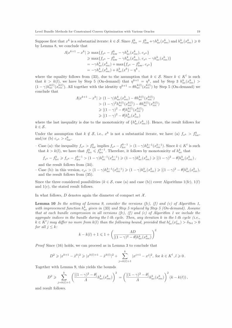
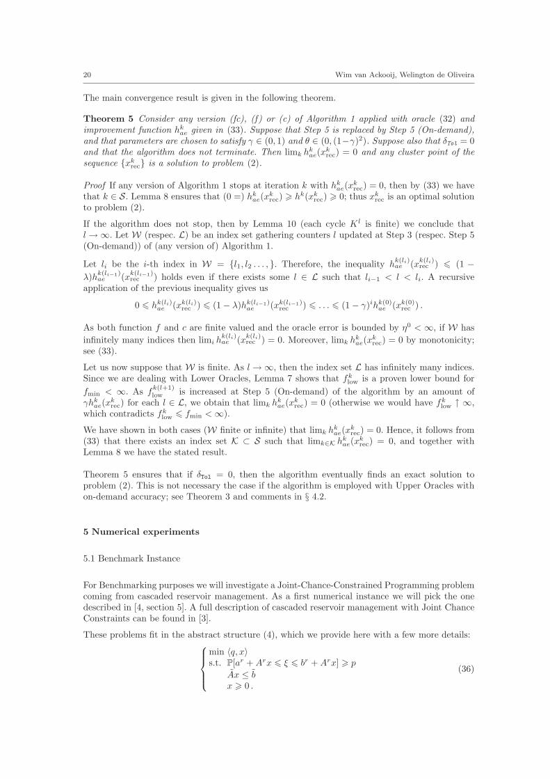
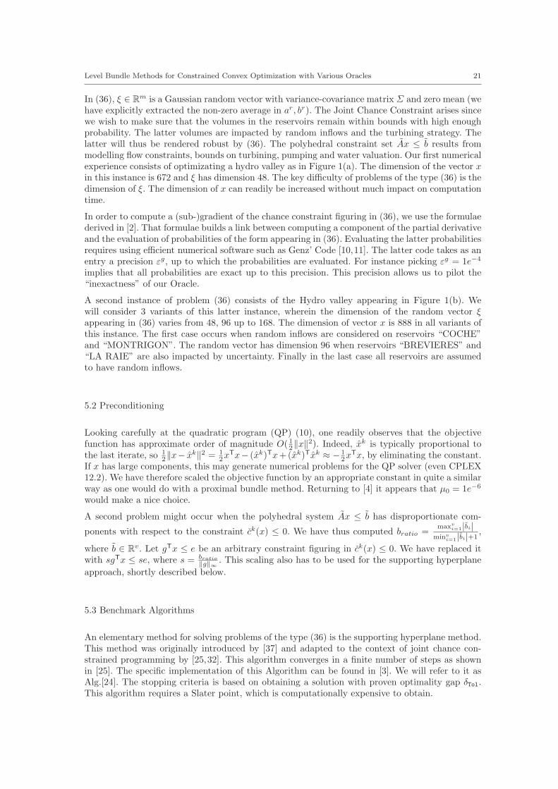
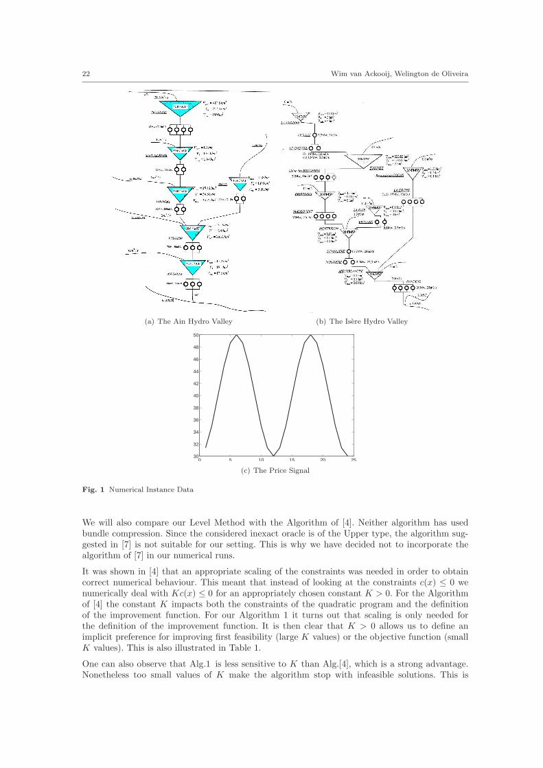
have explicitly extracted the non-zero average in ar, br). The Joint Chance Constraint arises sincewe wish to make sure that the volumes in the reservoirs remain within bounds with high enoughprobability. The latter volumes are impacted by random inflows and the turbining strategy. Thelatter will thus be rendered robust by (36). The polyhedral constraint set Ax ≤ b results frommodelling flow constraints, bounds on turbining, pumping and water valuation. Our first numericalexperience consists of optimizating a hydro valley as in Figure 1(a). The dimension of the vector xin this instance is 672 and ξ has dimension 48. The key difficulty of problems of the type (36) is thedimension of ξ. The dimension of x can readily be increased without much impact on computationtime.
In order to compute a (sub-)gradient of the chance constraint figuring in (36), we use the formulaederived in [2]. That formulae builds a link between computing a component of the partial derivativeand the evaluation of probabilities of the form appearing in (36). Evaluating the latter probabilitiesrequires using efficient numerical software such as Genz’ Code [10,11]. The latter code takes as anentry a precision εg, up to which the probabilities are evaluated. For instance picking εg = 1e−4
implies that all probabilities are exact up to this precision. This precision allows us to pilot the“inexactness” of our Oracle.
A second instance of problem (36) consists of the Hydro valley appearing in Figure 1(b). Wewill consider 3 variants of this latter instance, wherein the dimension of the random vector ξappearing in (36) varies from 48, 96 up to 168. The dimension of vector x is 888 in all variants ofthis instance. The first case occurs when random inflows are considered on reservoirs “COCHE”and “MONTRIGON”. The random vector has dimension 96 when reservoirs “BREVIERES” and“LA RAIE” are also impacted by uncertainty. Finally in the last case all reservoirs are assumedto have random inflows.
5.2 Preconditioning
Looking carefully at the quadratic program (QP) (10), one readily observes that the objectivefunction has approximate order of magnitude O( 1
2‖x‖2). Indeed, xk is typically proportional to
the last iterate, so 12‖x− xk‖2 = 1
2xTx− (xk)Tx+(xk)Txk ≈ − 12xTx, by eliminating the constant.
If x has large components, this may generate numerical problems for the QP solver (even CPLEX12.2). We have therefore scaled the objective function by an appropriate constant in quite a similarway as one would do with a proximal bundle method. Returning to [4] it appears that µ0 = 1e−6
would make a nice choice.
A second problem might occur when the polyhedral system Ax ≤ b has disproportionate com-
ponents with respect to the constraint ck(x) ≤ 0. We have thus computed bratio =maxv
i=1|bi|minv
i=1|bi|+1,
where b ∈ Rv. Let gTx ≤ e be an arbitrary constraint figuring in ck(x) ≤ 0. We have replaced it
with sgTx ≤ se, where s = bratio
‖g‖∞
. This scaling also has to be used for the supporting hyperplane
approach, shortly described below.
5.3 Benchmark Algorithms
An elementary method for solving problems of the type (36) is the supporting hyperplane method.This method was originally introduced by [37] and adapted to the context of joint chance con-strained programming by [25,32]. This algorithm converges in a finite number of steps as shownin [25]. The specific implementation of this Algorithm can be found in [3]. We will refer to it asAlg.[24]. The stopping criteria is based on obtaining a solution with proven optimality gap δTol.This algorithm requires a Slater point, which is computationally expensive to obtain.
22 Wim van Ackooij, Welington de Oliveira
(a) The Ain Hydro Valley (b) The Isere Hydro Valley
0 5 10 15 20 2530
32
34
36
38
40
42
44
46
48
50
(c) The Price Signal
Fig. 1 Numerical Instance Data
We will also compare our Level Method with the Algorithm of [4]. Neither algorithm has usedbundle compression. Since the considered inexact oracle is of the Upper type, the algorithm sug-gested in [7] is not suitable for our setting. This is why we have decided not to incorporate thealgorithm of [7] in our numerical runs.
It was shown in [4] that an appropriate scaling of the constraints was needed in order to obtaincorrect numerical behaviour. This meant that instead of looking at the constraints c(x) ≤ 0 wenumerically deal with Kc(x) ≤ 0 for an appropriately chosen constant K > 0. For the Algorithmof [4] the constant K impacts both the constraints of the quadratic program and the definitionof the improvement function. For our Algorithm 1 it turns out that scaling is only needed forthe definition of the improvement function. It is then clear that K > 0 allows us to define animplicit preference for improving first feasibility (large K values) or the objective function (smallK values). This is also illustrated in Table 1.
One can also observe that Alg.1 is less sensitive to K than Alg.[4], which is a strong advantage.Nonetheless too small values of K make the algorithm stop with infeasible solutions. This is
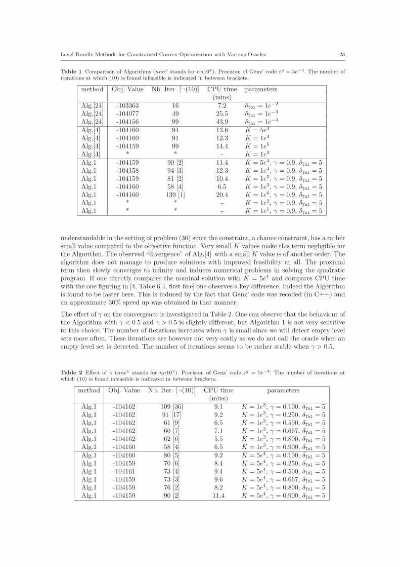
Level Bundle Methods for Constrained Convex Optimization with Various Oracles 23
Table 1 Comparison of Algorithms (nnex stands for nn10x). Precision of Genz’ code ε
g = 5e−4. The number of
iterations at which (10) is found infeasible is indicated in between brackets.
method Obj. Value Nb. Iter. [¬(10)] CPU time parameters(mins)
Alg.[24] -103363 16 7.2 δTol = 1e−2
Alg.[24] -104077 49 25.5 δTol = 1e−3
Alg.[24] -104156 99 43.9 δTol = 1e−4
Alg.[4] -104160 94 13.6 K = 5e4
Alg.[4] -104160 91 12.3 K = 1e4
Alg.[4] -104159 99 14.4 K = 1e5
Alg.[4] * * - K = 1e3
Alg.1 -104159 90 [2] 11.4 K = 5e4, γ = 0.9, δTol = 5Alg.1 -104158 94 [3] 12.3 K = 1e4, γ = 0.9, δTol = 5Alg.1 -104159 81 [2] 10.4 K = 1e5, γ = 0.9, δTol = 5Alg.1 -104160 58 [4] 6.5 K = 1e3, γ = 0.9, δTol = 5Alg.1 -104160 139 [1] 20.4 K = 1e6, γ = 0.9, δTol = 5Alg.1 * * - K = 1e2, γ = 0.9, δTol = 5Alg.1 * * - K = 1e1, γ = 0.9, δTol = 5
understandable in the setting of problem (36) since the constraint, a chance constraint, has a rathersmall value compared to the objective function. Very small K values make this term negligible forthe Algorithm. The observed “divergence” of Alg.[4] with a small K value is of another order. Thealgorithm does not manage to produce solutions with improved feasibility at all. The proximalterm then slowly converges to infinity and induces numerical problems in solving the quadraticprogram. If one directly compares the nominal solution with K = 5e4 and compares CPU timewith the one figuring in [4, Table 6.4, first line] one observes a key difference. Indeed the Algorithmis found to be faster here. This is induced by the fact that Genz’ code was recoded (in C++) andan approximate 30% speed up was obtained in that manner.
The effect of γ on the convergence is investigated in Table 2. One can observe that the behaviour ofthe Algorithm with γ < 0.5 and γ > 0.5 is slightly different, but Algorithm 1 is not very sensitiveto this choice. The number of iterations increases when γ is small since we will detect empty levelsets more often. These iterations are however not very costly as we do not call the oracle when anempty level set is detected. The number of iterations seems to be rather stable when γ > 0.5.
Table 2 Effect of γ (nnex stands for nn10x). Precision of Genz’ code ε
g = 5e−4. The number of iterations at
which (10) is found infeasible is indicated in between brackets.
method Obj. Value Nb. Iter. [¬(10)] CPU time parameters(mins)
Alg.1 -104162 109 [36] 9.1 K = 1e3, γ = 0.100, δTol = 5Alg.1 -104162 91 [17] 9.2 K = 1e3, γ = 0.250, δTol = 5Alg.1 -104162 61 [9] 6.5 K = 1e3, γ = 0.500, δTol = 5Alg.1 -104162 60 [7] 7.1 K = 1e3, γ = 0.667, δTol = 5Alg.1 -104162 62 [6] 5.5 K = 1e3, γ = 0.800, δTol = 5Alg.1 -104160 58 [4] 6.5 K = 1e3, γ = 0.900, δTol = 5Alg.1 -104160 80 [5] 9.2 K = 5e4, γ = 0.100, δTol = 5Alg.1 -104159 70 [6] 8.4 K = 5e4, γ = 0.250, δTol = 5Alg.1 -104161 73 [4] 9.4 K = 5e4, γ = 0.500, δTol = 5Alg.1 -104159 73 [3] 9.6 K = 5e4, γ = 0.667, δTol = 5Alg.1 -104159 76 [2] 8.2 K = 5e4, γ = 0.800, δTol = 5Alg.1 -104159 90 [2] 11.4 K = 5e4, γ = 0.900, δTol = 5
24 Wim van Ackooij, Welington de Oliveira
In the standard variant of Alg.1 the level set (9) is detected to be empty when the quadratic solverattempting to solve (10) produces an infeasible solution. The lower bound fk
low is then updated.Alternatively the lower bound can be updated by solving the additional linear program (17) in Step5 of Algorithm 1. Since in these numerical experiments there is no bundle compression, solving(17) at each iteration does not impact the convergence analysis of the algorithm; see comment (f)after Algorithm 1. The effect of this choice is reported in Table 3. In the setting of problem (36)the c-oracle is costly to call and hence solving an additional linear program (or even quadraticprogram) has a negligible effect on computation time. A further effect of adding (17) to step 5 ofthe Algorithm is that (9) will never be empty anymore.
Table 3 Effect of adding (17) to Step 5. (nnex stands for nn10x). Precision of Genz’ code ε
g = 5e−4.
method Obj. Value Nb. Iter. CPU time parameters(mins)
Alg.1 -104161 35 4.4 K = 1e3, γ = 0.8, δTol = 5Alg.1 -104158 65 9.2 K = 5e4, γ = 0.8, δTol = 5
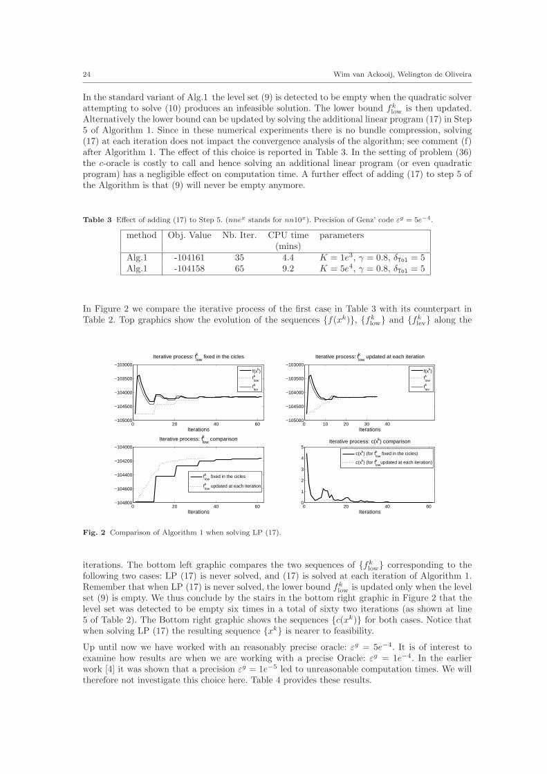
In Figure 2 we compare the iterative process of the first case in Table 3 with its counterpart inTable 2. Top graphics show the evolution of the sequences {f(xk)}, {fk
low} and {fklev} along the
0 20 40 60−105000
−104500
−104000
−103500
−103000
Iterations
Iterative process: fklow
fixed in the cicles
f(xk)
fklow
fklev
0 10 20 30 40−105000
−104500
−104000
−103500
−103000
Iterations
Iterative process: fklow
updated at each iteration
f(xk)
fklow
fklev
0 20 40 60−104800
−104600
−104400
−104200
−104000
Iterations
Iterative process: fklow
comparison
fklow
fixed in the cicles
fklow
updated at each iteration
0 20 40 600
1
2
3
4
5
Iterations
Iterative process: c(xk) comparison
c(xk) (for fklow
fixed in the cicles)
c(xk) (for fklow
updated at each iteration)
Fig. 2 Comparison of Algorithm 1 when solving LP (17).
iterations. The bottom left graphic compares the two sequences of {fklow} corresponding to the
following two cases: LP (17) is never solved, and (17) is solved at each iteration of Algorithm 1.Remember that when LP (17) is never solved, the lower bound fk
low is updated only when the levelset (9) is empty. We thus conclude by the stairs in the bottom right graphic in Figure 2 that thelevel set was detected to be empty six times in a total of sixty two iterations (as shown at line5 of Table 2). The Bottom right graphic shows the sequences {c(xk)} for both cases. Notice thatwhen solving LP (17) the resulting sequence {xk} is nearer to feasibility.
Up until now we have worked with an reasonably precise oracle: εg = 5e−4. It is of interest toexamine how results are when we are working with a precise Oracle: εg = 1e−4. In the earlierwork [4] it was shown that a precision εg = 1e−5 led to unreasonable computation times. We willtherefore not investigate this choice here. Table 4 provides these results.
Level Bundle Methods for Constrained Convex Optimization with Various Oracles 25
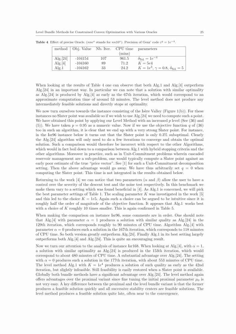
Table 4 Effect of precise Oracle. (nnex stands for nn10x). Precision of Genz’ code ε
g = 1e−4.
method Obj. Value Nb. Iter. CPU time parameters(mins)
Alg.[24] -104154 107 961.5 δTol = 1e−4
Alg.[4] -104160 89 71.2 K = 5e4Alg.1 -104162 33 24.2 K = 1e3, γ = 0.8, δTol = 5
When looking at the results of Table 4 one can observe that both Alg.1 and Alg.[4] outperformAlg.[24] in an important way. In particular we can note that a solution with similar optimalityas Alg.[24] is produced by Alg.[4] as early as the 67th iteration, which would correspond to anapproximate computation time of around 53 minutes. The level method does not produce anyintermediately feasible solutions and directly stops at optimality.
We now turn ourselves towards the instance consisting of the Isere Valley (Figure 1(b)). For theseinstances no Slater point was available so if we wish to use Alg.[24] we need to compute such a point.We have obtained this point by applying our Level Method with an increased p level (See (36) and(5)). We have taken p = 0.95 as a numeric value. Now if we use the objective function q of (36)too in such an algorithm, it is clear that we end up with a very strong Slater point. For instance,in the Isr96 instance below it turns out that the Slater point is only 0.3% suboptimal. Clearlythe Alg.[24] algorithm will only need to do a few iterations to converge and obtain the optimalsolution. Such a comparison would therefore be incorrect with respect to the other Algorithms,which would in fact boil down to a comparison between Alg.1 with hybrid stopping criteria and theother algorithms. Moreover in practice, such as in Unit-Commitment problems wherein cascadedreservoir management are a sub-problem, one would typically compute a Slater point against anearly poor estimate of the true “price vector”. See [1] for such a Unit-Commitment decompositionsetting. Then the above advantage would go away. We have thus arbitrarily set q = 0 whencomputing the Slater point. This time is not integrated in the results obtained below.
Returning to the work [4] we can notice that two parameters (α and β) allow the user to have acontrol over the severity of the descent test and the noise test respectively. In this benchmark wemake them vary to a setting which was found beneficial in [4]. As Alg.1 is concerned, we will pickthe best parameter settings of Table 1. The scaling parameter K was investigated in the work [5]and this led to the choice K = 1e5. Again such a choice can be argued to be intuitive since it isroughly half the order of magnitude of the objective function. It appears that Alg.1 works bestwith a choice of K roughly 10 times smaller. This is again confirmed in Table 5.
When making the comparison on instance Isr96, some comments are in order. One should notethat Alg.[4] with parameter α = 1 produces a solution with similar quality as Alg.[24] in the129th iteration, which corresponds roughly to 90 minutes of CPU time. Algorithm Alg.[4] withparameter α = 0 produces such a solution in the 167th iteration, which corresponds to 118 minutesof CPU time. So both version greatly outperform Alg.[24]. Finally Alg.1 in its best setting largelyoutperforms both Alg.[4] and Alg.[24]. This is quite an encouraging result.
Now we turn our attention to the analysis of instance Isr168. When looking at Alg.[4], with α = 1,a solution with similar optimality as Alg.[24] is produced in the 153th iteration, which wouldcorrespond to about 480 minutes of CPU time. A substantial advantage over Alg.[24]. The settingwith α = 0 produces such a solution in the 177th iteration, with about 553 minutes of CPU time.The level method Alg.1 with K = 1e4 produces a solution of such quality as early as the 42nditeration, but slightly infeasible. Still feasibility is easily restored when a Slater point is available.Globally both bundle methods have a significant advantage over Alg.[24]. The level method againoffers advantages over the proximal variant since fine tuning the initial proximal parameter µ0 isnot very easy. A key difference between the proximal and the level bundle variant is that the formerproduces a feasible solution quickly and all successive stability centers are feasible solutions. Thelevel method produces a feasible solution quite late, often near to the convergence.
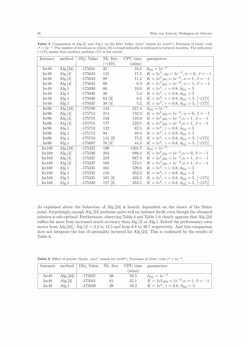
26 Wim van Ackooij, Welington de Oliveira
Table 5 Comparison of Alg.[4] and Alg.1 on the Isere Valley. (nnex stands for nn10x). Precision of Genz’ code
εg = 5e
−4. The number of iterations at which (10) is found infeasible is indicated in between brackets. The indication[¬(17)] means that auxiliary problem (17) is not solved.
Instance method Obj. Value Nb. Iter. CPU time parameters[¬(10)] (mins)
Isr48 Alg.[24] -175031 35 10.5 δTol = 1e−4
Isr48 Alg.[4] -175043 115 17.5 K = 1e5, µ0 = 1e−5, α = 0, β = −1Isr48 Alg.[4] -175043 88 11.2 K = 1e5,µ0 = 1e−5, α = 1, β = −1Isr48 Alg.[4] -175042 69 8.3 K = 1e5,µ0 = 1e−6, α = 1, β = −1Isr48 Alg.1 -175039 66 10.0 K = 1e5, γ = 0.8, δTol = 5Isr48 Alg.1 -175040 38 5.4 K = 1e4, γ = 0.8, δTol = 5Isr48 Alg.1 -175040 63 [3] 8.6 K = 1e5, γ = 0.8, δTol = 5, [¬(17)]Isr48 Alg.1 -175037 38 [4] 5.2 K = 1e4, γ = 0.8, δTol = 5, [¬(17)]Isr96 Alg.[24] -175708 143 217.4 δTol = 1e−4
Isr96 Alg.[4] -175714 214 152.3 K = 1e5,µ0 = 1e−5, α = 0, β = −1Isr96 Alg.[4] -175715 159 110.9 K = 1e5,µ0 = 1e−5,α = 1, β = −1Isr96 Alg.[4] -175715 177 123.5 K = 1e5,µ0 = 1e−6,α = 1, β = −1Isr96 Alg.1 -175713 122 82.5 K = 1e5, γ = 0.8, δTol = 5Isr96 Alg.1 -175713 94 48.4 K = 1e4, γ = 0.8, δTol = 5Isr96 Alg.1 -175710 115 [3] 75.3 K = 1e5, γ = 0.8, δTol = 5, [¬(17)]Isr96 Alg.1 -175697 76 [4] 44.3 K = 1e4, γ = 0.8, δTol = 5, [¬(17)]Isr168 Alg.[24] -175222 190 1504.7 δTol = 1e−4
Isr168 Alg.[4] -175236 284 888.4 K = 1e5,µ0 = 1e−5,α = 0, β = −1Isr168 Alg.[4] -175237 219 687.4 K = 1e5,µ0 = 1e−5,α = 1, β = −1Isr168 Alg.[4] -175237 188 573.5 K = 1e5,µ0 = 1e−6,α = 1, β = −1Isr168 Alg.1 -175235 161 529.6 K = 1e5, γ = 0.8, δTol = 5Isr168 Alg.1 -175232 110 352.3 K = 1e4, γ = 0.8, δTol = 5Isr168 Alg.1 -175235 165 [3] 423.2 K = 1e5, γ = 0.8, δTol = 5, [¬(17)]Isr168 Alg.1 -175220 127 [5] 353.5 K = 1e4, γ = 0.8, δTol = 5, [¬(17)]
As explained above the behaviour of Alg.[24] is heavily dependent on the choice of the Slaterpoint. Surprisingly enough Alg.[24] performs quite well on instance Isr48, even though the obtainedsolution is sub-optimal. Furthermore, observing Table 4 and Table 1 it clearly appears that Alg.[24]suffers far more from increased oracle accuracy than Alg.[4] or Alg.1. Indeed the performance ratiomoves from Alg.[24]/ Alg.[4] = 3.2 to 13.5 and from 6.8 to 39.7 respectively. And this comparisondoes not integrate the loss of optimality incurred for Alg.[24]. This is confirmed by the results ofTable 6.
Table 6 Effect of precise Oracle. (nnex stands for nn10x). Precision of Genz’ code ε
g = 1e−4.
Instance method Obj. Value Nb. Iter. CPU time parameters(mins)
Isr48 Alg.[24] -175037 39 58.5 δTol = 1e−4
Isr48 Alg.[4] -175041 81 35.1 K = 1e5,µ0 = 1e−6,α = 1, β = −1Isr48 Alg.1 -175039 39 16.2 K = 1e4, γ = 0.8, δTol = 5
Level Bundle Methods for Constrained Convex Optimization with Various Oracles 27
5.4 Comments on Parameter Settings
The previous subsection was devoted to a comparison of Bundle Methods and the SupportingHyperplane method for solving convex joint chance constrained programs. The latter methodrequires a Slater point, which might be tricky to obtain, but on the other hand the methodhas few parameters. This can be perceived as an advantage, since one might be afraid to have tospend much time in setting up appropriate choices. However this is untrue, since natural parameterchoices for the Bundle methods led to good results. Indeed, both Bundle Methods have parametersettings to play with. The proximal variant, has choices for the definition of the nominal decrease,the noise test, the “magic” scaling parameter K and the initial proximal parameter µ0. The LevelMethod also has the scaling parameter K, γ and the stopping tolerance to set. We have howevershown that results are relatively robust to changes in such parameters provided they are in theright zone. Also when moving from one instance to another (both coming from cascaded reservoirmanagement) the same rules of thumb seem to give quite excellent initial choices. Globally for jointchance constraint programming we would suggest to solve the following deterministic equivalentof (36):
min 〈q, x〉s.t. ar + Arx 6 0
0 6 br + Arx
Ax ≤ bx > 0
(37)
and call xd its optimal solution. Then f0low =
⟨
q, xd⟩
is a good lower bound for (36), K = 12
⟨
q, xd⟩
an appropriate choice for the magic Scaling parameter in the proximal Bundle Method. For thelevel method we should pick around 1
10 th of that value. The initial proximal parameter shouldbe set up according to what has been explained in section 5.2. According to our experience thequadratic term ‖x− xk‖2 should not exceed 1e11 and µ0 can be set accordingly.
6 Conclusions
In this work we have proposed a class of nonlinear constrained level bundle methods for convexnonsmooth optimization. The proposed algorithms can deal with exact, inexact (of Upper andLower type) and on-demand accuracy oracles. Such methods are readily implementable and re-quire, in addition to convexity, only the additional compactness assumption. The latter is readilyavailable in engineering problems. By assuming the existence of a Slater point, a variant of themethod capable of dealing with Upper oracles with on-demand accuracy is suggested as well. Thisis a new and interesting kind of oracle suitable for difficult-to-evaluate functions for the which onewishes to find (with reasonable CPU time) an approximate minimizer of good quality.
We emphasize that all proposed variants are of restricted-memory type: the bundle of informationused to build the cutting-plane models (approximating the constraint and objective functions)can be kept bounded, having for instance only four linearizations. This is an important feature forusing computer memory wisely. It also helps to keep the quadratic problem as small as one wishes.Although this feature appears in [15], it is not present in the inexact versions of constrained levelbundle methods proposed in [9] and [7].
In addition to the convergence analysis of all proposed variants, complexity results are also given.We can derive the same complexity results if we skip, in an appropriate way, a call to the oraclefor either the objective or constraint function. Such a feature is of interest if either one of theseoracles is expensive. The proposed variants of our algorithms avoid calling one of these oracles ifthe current iterate does not provide enough improvement towards a solution of the problem. Thisis an useful feature that was not present in the literature of the constrained level bundle methods.
28 Wim van Ackooij, Welington de Oliveira
As already mentioned, one important advantage of constrained level bundle methods over con-strained proximal bundle methods is the easily defined improvement function. Level bundle meth-ods have at disposal lower bounds (self-built) to define such an improvement function, useful tomeasure the improvement of each iterate towards a solution to the problem. In contrast, proximalbundle methods must find other definitions of the improvement function, since lower bounds forthe optimal value are, in general, not available. Moreover, the latter class of methods use the con-cept of serious and null steps, that are classified according to the “faulty” improvement function.Serious steps are set as stability centers for the proximal bundle methods, and their classificationis crucial for the efficiency of the algorithm. None of the proposed level method variants employsthe idea of serious and null steps. Moreover, the stability center (projection point) for the givenvariants can be any point in the bundle (e.g., the initial point). This is another advantage of thelevel variant over the proximal one: no special attention needs to be given to the choice of stabilitycenters. Therefore, from the theoretical point of view, we can conclude that the level variant islikely to be preferable than the proximal one to solve nonlinear constraint convex optimizationproblems. This conclusion is also supported by our numerical experiments.
We carried out numerical experiments on realistic joint chance constrained energy problems, arisingwhen dealing with robust cascaded-reservoir management. On several instances of the problem, wehave compared our algorithm with a supporting hyperplane method and a performant proximalbundle method.
Numerical results show that globally the bundle (level and proximal) variants greatly outperformthe supporting hyperplane algorithm. Moreover, our level variant outperforms the proximal bundlealgorithm. For the most difficult instance of the considered problem (Isr168, whose CPU timespent to compute an inexact oracle information is around three minutes), the proximal bundle inits best setting provides a reduction in CPU time of around 61%, when compared to the supportinghyperplane algorithm. When using the best setting of the level variant, the reduction in CPU timeis around 76%. This is a very promising improvement (the level algorithm solves the problem inslightly more than 5 hours, while the supporting hyperplane algorithm needs more than 25 hours).
Another observed difference between the proximal and the level bundle variant is that the formerproduces a feasible solution quickly and all successive stability centers are feasible solutions. Thelevel algorithm produces a feasible solution quite late, often near convergence.
Finally, it was shown by our numerical experiments that solving a linear problem at each itera-tion to avoid empty level sets decreases the total number of iterations. While this strategy hasbeen very effective in some cases, we cannot ensure that it will be in general: the computationalburden increases at each iteration. It is worthy mentioning that solving such linear programmingis optional for the proposed variants, but it is mandatory for earlier published constrained levelbundle algorithms.
[36,29]
References
1. van Ackooij, W.: Decomposition approaches for block-structured chance-constrained programs with applicationto hydro-thermal unit-commitment. Submitted ; Preprint CR-2012-08 (2012). URL http://www.lgi.ecp.fr/
Biblio/PDF/CR-LGI-2012-08.pdf2. van Ackooij, W., Henrion, R., Moller, A., Zorgati, R.: On probabilistic constraints induced by rectangular sets
and multivariate normal distributions. Mathematical Methods of Operations Research 71(3), 535–549 (2010)3. van Ackooij, W., Henrion, R., Moller, A., Zorgati, R.: Joint chance constrained programming for hydro reser-
voir management. Draft submitted; Preprint DFG Matheon #862 (2011). URL http://opus4.kobv.de/
opus4-matheon/frontdoor/index/index/docId/9924. van Ackooij, W., Sagastizabal, C.: Constrained bundle methods for upper inexact oracles with application
to joint chance constrained energy problems. Submitted; Preprint available at http://www.optimization-online.org/DB HTML/2012/12/3711.html pp. 1–25 (2012)
5. van Ackooij, W., Zorgati, R.: Estimating the probabilistic contents of gaussian rectangles faster in joint chanceconstrained programming for hydro reservoir management. EngOpt2012, 3rd International Conference onEngineering optimization (2012)
Level Bundle Methods for Constrained Convex Optimization with Various Oracles 29
6. Dentcheva, D., Martinez, G.: Two-stage stochastic optimization problems with stochastic ordering constraintson the recourse. European Journal of Operational Research 219(1), 1–8 (2012)
7. Fabian, C.: Computational aspects of risk-averse optimisation in two-stage stochastic models. Tech. rep. (2013).URL http://www.optimization-online.org/DB_HTML/2012/08/3574.html. Optimization Online report
8. Fabian, C., Szoke, Z.: Solving two-stage stochastic programming problems with level decomposition. Compu-tational Management Science 4, 313–353 (2007)
9. Fabian, C.I.: Bundle-type methods for inexact data. In: Proceedings of the XXIV Hungarian OperationsResearc Conference (Veszprem, 1999), vol. 8 (special issue, T. Csendes and T. Rapcsk, eds.), pp. 35–55 (2000)
10. Genz, A.: Numerical computation of multivariate normal probabilities. J. Comp. Graph Stat. 1, 141–149 (1992)11. Genz, A., Bretz, F.: Computation of multivariate normal and t probabilities. No. 195 in Lecture Notes in
Statistics. Springer, Dordrecht (2009)12. Hintermuller, M.: A proximal bundle method based on approximate subgradients. Computational Op-
timization and Applications 20, 245–266 (2001). URL http://dx.doi.org/10.1023/A:1011259017643.10.1023/A:1011259017643
13. Hiriart-Urruty, J., Lemarechal, C.: Convex Analysis and Minimization Algorithms II. No. 306 in Grundlehrender mathematischen Wissenschaften, 2nd edn. Springer-Verlag (1996)
14. Karas, E., Ribeiro, A., Sagastizabal, C., Solodov, M.: A bundle-filter method for nonsmooth convex constrainedoptimization. Math. Program. 116(1), 297–320 (2008). DOI 10.1007/s10107-007-0123-7. URL http://dx.doi.
org/10.1007/s10107-007-0123-7
15. Kiwiel, K.: Proximal level bundle methods for convex nondifferentiable optimization, saddle-point problemsand variational inequalities. Math. Programming 69(1), 89–109 (1995)
16. Kiwiel, K.: A proximal bundle method with approximate subgradient linearizations. SIAM Journal on Opti-mization 16(4), 1007–1023 (2006)
17. Kiwiel, K.: An inexact bundle approach to cutting stock problems. Informs Journal on Computing 22, 131–143(2010)
18. Kiwiel, K., Lemarechal, C.: An inexact bundle variant suited to column generation. Math. Program. 118(1),177–206 (2009)
19. Lemarechal, C., Nemirovskii, A., Nesterov, Y.: New variants of bundle methods. Math. Programming 69(1),111–147 (1995)
20. Oliveira, W., Sagastizabal, C.: Level bundle methods for oracles with on demand accuracy. Available athttp://www.optimization-online.org/DB HTML/2012/03/3390.html (2012)
21. Oliveira, W., Sagastizabal, C., Lemarechal, C.: Bundle methods in depth: a unified analysis for inexact oracles.Available at http://www.optimization-online.org/DB HTML/2013/02/3792.html (2013)
22. Oliveira, W., Sagastizbal, C.A., Scheimberg, S.: Inexact bundle methods for two-stage stochastic programming.SIAM Journal on Optimization 21(2), 517–544 (2011). DOI http://dx.doi.org/10.1137/100808289
23. Prekopa, A.: Stochastic Programming. Kluwer, Dordrecht (1995)24. Prekopa, A.: Probabilistic programming. In [29] (Chapter 5). Elsevier, Amsterdam (2003)25. Prekopa, A., Szantai, T.: Flood control reservoir system design using stochastic programming. Math. Program-
ming Study 9, 138–151 (1978)26. Rockafellar, R.: Convex Analysis. 1st edn. Princeton University Press (1970)27. Rockafellar, R., Uryas’ev, S.: Optimization of conditional value-at-risk. Journal of risk 2, 21–42 (2000)28. Rockafellar, R., Uryas’ev, S.: Conditional value at risk: optimization approach. Stochastic optimization: algo-
rithms and applications pp. 411–435 (2001)29. Ruszczynski, A., Shapiro, A.: Stochastic Programming, Handbooks in Operations Research and Management
Science, vol. 10. Elsevier, Amsterdam (2003)30. Sagastizabal, C., Solodov, M.: An infeasible bundle method for nonsmooth convex constrained optimization
without a penalty function or a filter. SIAM Journal on Optimization 16(1), 146–169 (2005). URL http:
//siamdl.aip.org/dbt/dbt.jsp?KEY=SJOPE8&Volume=16&Issue=1
31. Shapiro, A., Dentcheva, D., Ruszczynski, A.: Lectures on Stochastic Programming. Modeling and Theory,MPS-SIAM series on optimization, vol. 9. SIAM and MPS, Philadelphia (2009)
32. Szantai, T.: A computer code for solution of probabilistic-constrained stochastic programming problems. In(Y. Ermoliev and R.J.-B. Wets eds.): Numerical Techniques for Stochastic Optimization pp. 229–235 (1988)
33. Uryas’ev, S.: A differentation formula for integrals over sets given by inclusion. Numerical functional Analysisand Optimization 10(7&8), 827–841 (1989)
34. Uryas’ev, S.: Derivatives of probability functions and some applications. Annals of Operations Research 56,287–311 (1995)
35. Uryas’ev, S.: Introduction to the Theory of Probabilistic Functions and Percentiles (Value-at-Risk) Chapter 1in [36]. Kluwer Academic Publishers (2000)
36. Uryas’ev (ed), S.: Probabilistic Constrained Optimization: Methodology and Applications. Kluwer AcademicPublishers (2000)
37. Veinott, A.: The supporting hyperplane method for unimodal programming. Operations Research 15, 147–152(1967)