Embed Size (px)
Citation preview
Level Set Formulationfor Curve Evolution
Ron Kimmel
www.cs.technion.ac.il/~ron
Computer Science Department Technion-Israel Institute of Technology
Geometric Image Processing Lab
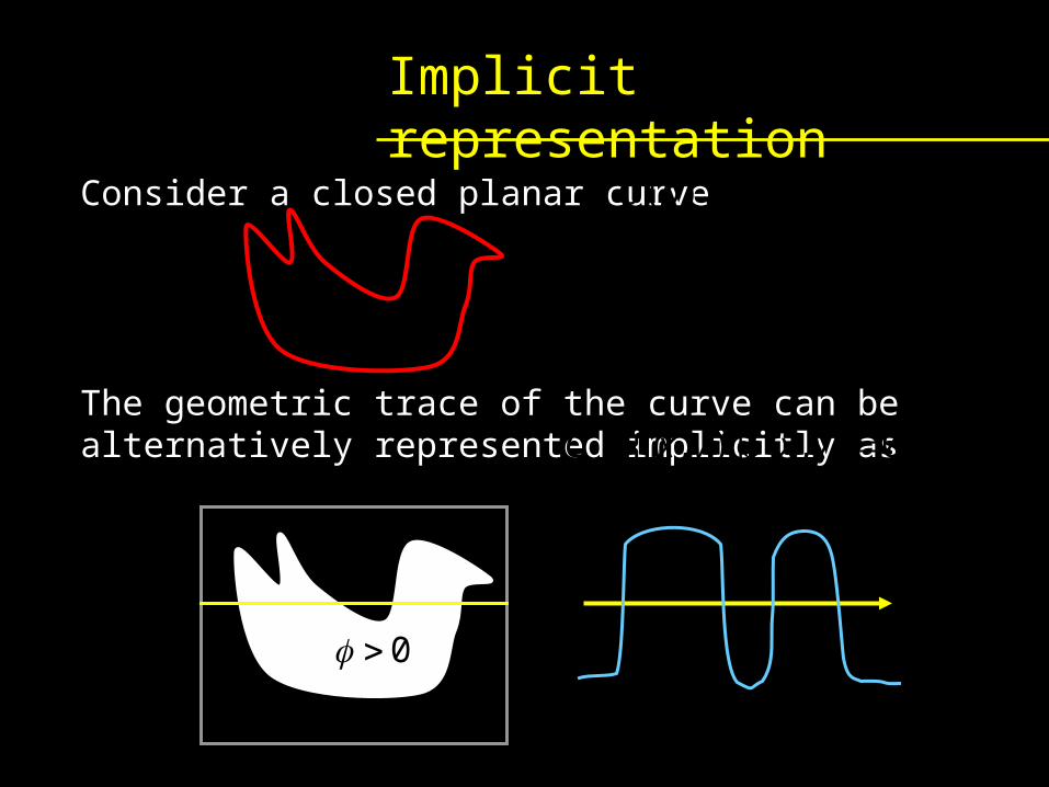
Consider a closed planar curve
The geometric trace of the curve can be alternatively represented implicitly as
Implicit representation21:)( RS pC
}0),(|),{( yxyxC
0
0
1
1
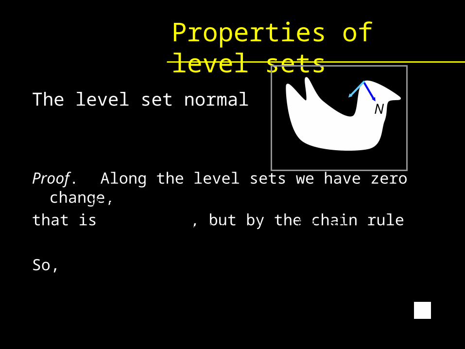
Properties of level sets
The level set normal
Proof. Along the level sets we have zero change,
that is , but by the chain rule
So,
||
N
N
0s
Tyxyx sysxs
,),(
T
||||0,
||
NTT
||
T
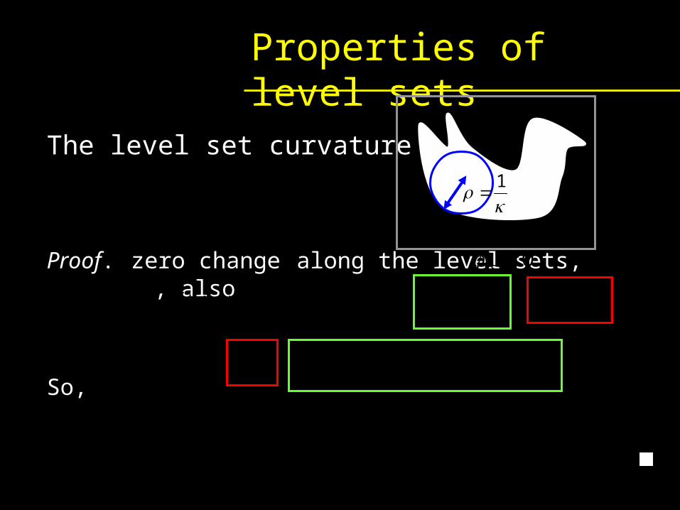
Properties of level sets
The level set curvature
Proof. zero change along the level sets, , also
So,
||
div
0ss
NTds
dT
ds
dyx
ds
dyx sysxss
,,,)(),(
...||
,||
,,||
,||
,,,,
||],,[||
||,
yxyx
syysxysxysxx
TT
yxyx
1
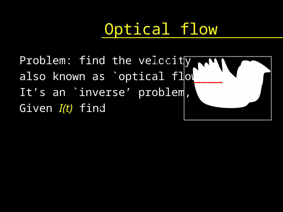
Optical flow
Problem: find the velocity also known as `optical flow’It’s an `inverse’ problem,Given I(t) find
VII t
,
),( yxV
),( yxV
VtxItxI
dtVdtdtVOVdttxItxdtItxItxI
dtVOVdtdttxIdttxItxI
dttVdtxItxI
t
t
),,(),(
0),,(),,(),(),(),(
0)(),,(),(),(
0),(),(
2222
22
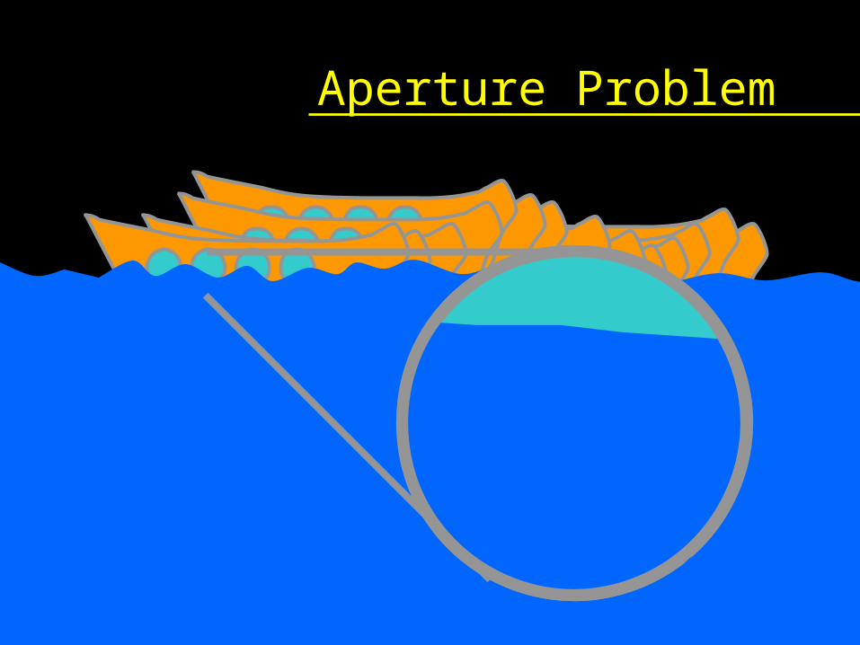
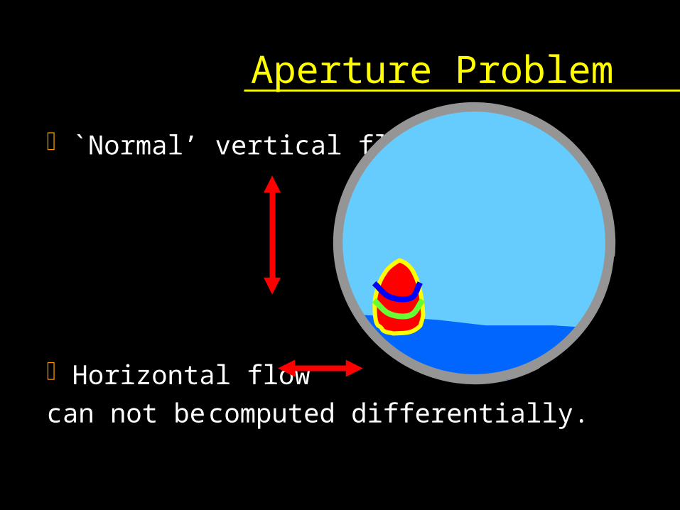
Aperture Problem
Aperture Problem
`Normal’ vertical flow
Horizontal flow can not be computed differentially.
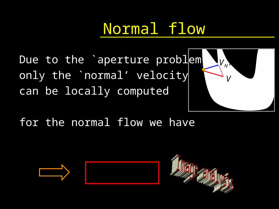
Normal flow
Due to the `aperture problem’only the `normal’ velocity can be locally computed
for the normal flow we have
V
||,
I
IVNNVNV NN
||||
,,, IVI
IIVNVIVII NNNt
NVN
|| IVI Nt
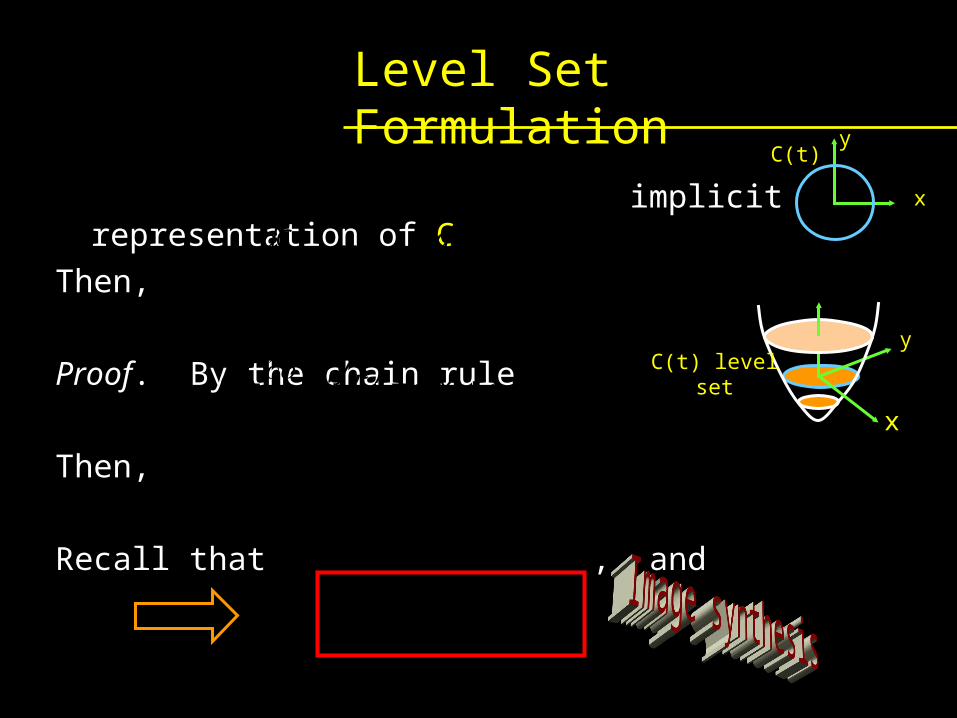
Level Set Formulation
implicit representation of CThen,
Proof. By the chain rule
Then,
Recall that , and
RR 2:, yx 0),(:, yxyxC
dC d
VN Vdt dt
ttytx yxt
tyx
);,(
0
y
x
C(t)
C(t) level set 0
, ,x y t
x
y
NVNVCyx ttytxt
,,,
||
N
||||
,,
VVNV
|| Vt
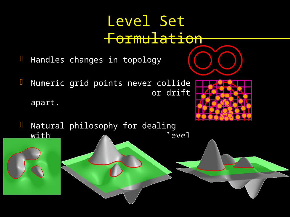
Level Set Formulation
Handles changes in topology
Numeric grid points never collide or drift apart.
Natural philosophy for dealing with gray level images.
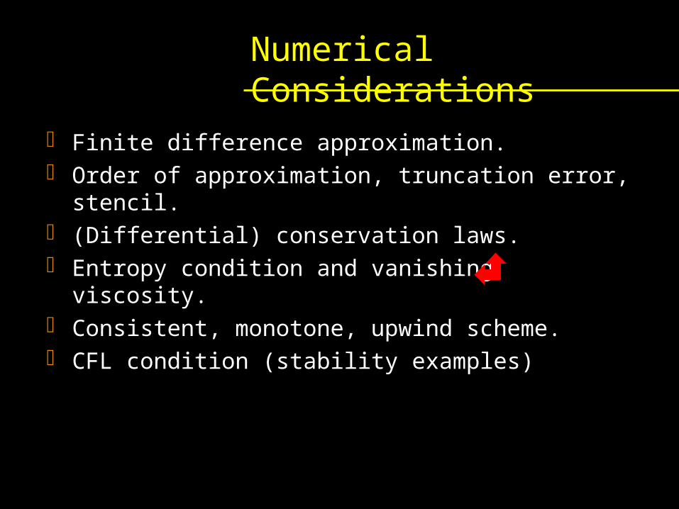
Numerical Considerations
Finite difference approximation. Order of approximation, truncation error, stencil. (Differential) conservation laws. Entropy condition and vanishing viscosity. Consistent, monotone, upwind scheme. CFL condition (stability examples)
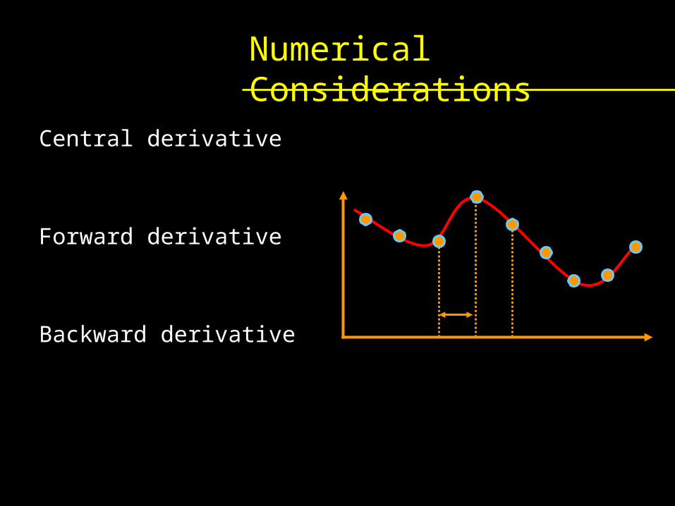
Numerical Considerations
Central derivative
Forward derivative
Backward derivative
)(ihuui )(xu
x
h
1 1 iii
h
uuuD ii
x 211
h
uuuD ii
x
1
h
uuuD ii
x1
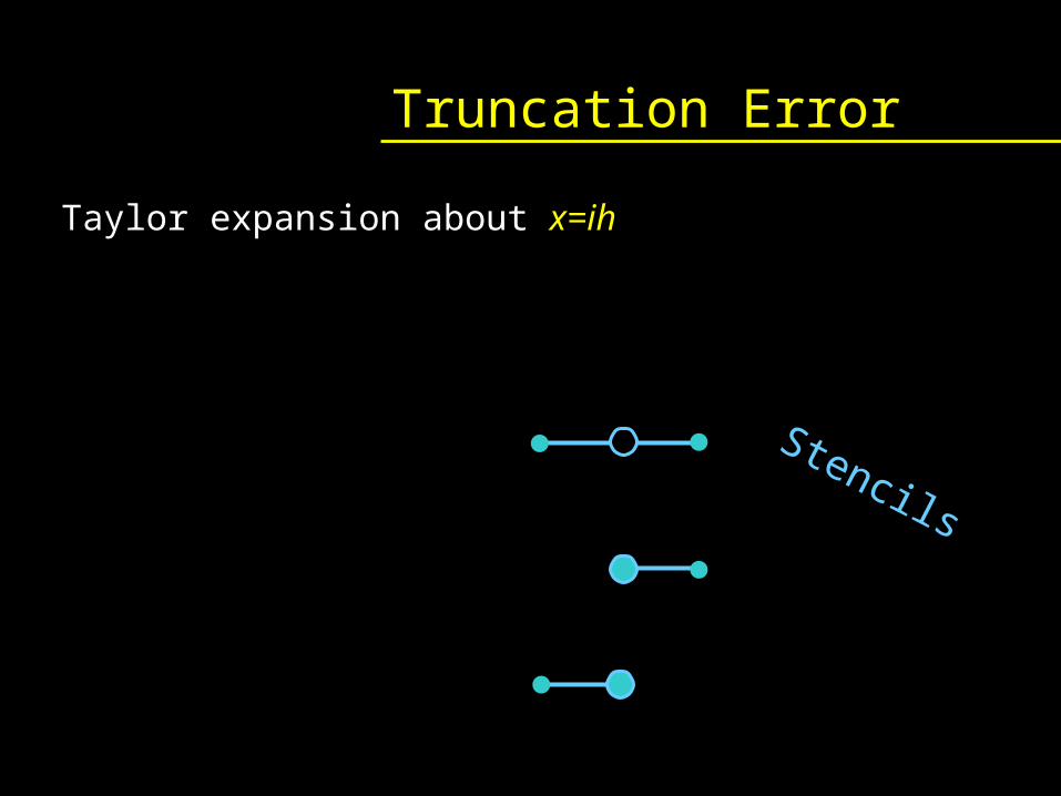
Truncation Error
Taylor expansion about x=ih
)()('
)()('
)()('
)()('')(')()(
)()('')(')()(
2
32!2
11
32!2
11
hOihuuD
hOihuuD
hOihuuD
hOihuhihhuihuhihuu
hOihuhihhuihuhihuu
ix
ix
ix
i
i
21
21
1 1
11
Stencils
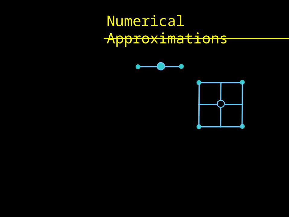
Numerical Approximations
2
1,11,11,11,1
4h
uuuuuD jijijiji
xy
211 2
h
uuuuD iii
xx
1 2- 1
41
41
41
41
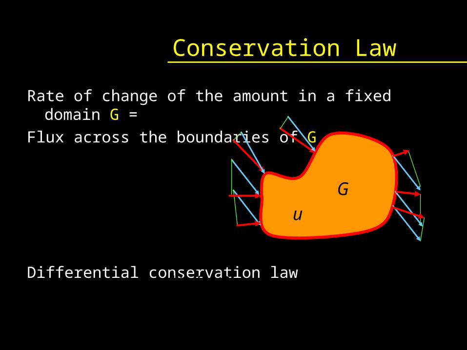
Conservation Law
Rate of change of the amount in a fixed domain G =
Flux across the boundaries of G
Differential conservation law
GG
dSnfudxdt
d ,
G
u
0 div fut
nnf
,
f
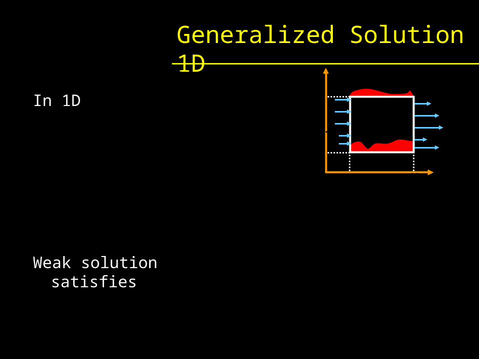
Generalized Solution 1D
In 1D
Weak solution satisfies
u
0),(),(),(),(
0
0 div
1
0
1
0
1
0
1
0
1
0
1
0
0101
dttxftxfdxtxutxu
dtdxfu
dtdxfu
t
t
x
x
t
t
x
x
xt
t
t
x
x
t
)),(()),((),( 10
1
0
txuHtxuHdxtxudt
dx
x
t
x
1t
0t
0x 1x
ff u
u

Hamilton-Jacobi
In 1D: HJ=Hyperbolic conservation lawsIn 2D: just the `flavor’…
Vanishing viscosity, of
The `entropy condition’ selected the `weak solution’
that is the `vanishing viscosity solution’ also known
as `entropy solution’.
xxxt uuHu )(0
lim
Nεκ
NCt
Numerical Schemes
Conservation form
Numerical flux
The scheme is monotone, if F is non-decreasing.
Theorem: A monotone, consistent scheme, in conservation form converges to the entropy solution.
Yet, up to 1st order accurate ;-( …
x
gg
t
uu nj
nj
nj
nj
2
12
11
),...,( 11 n
qjn
pjnj uuFu
)(),...,( ),,...,( 1121 uHuuguugg qjpj
nj

Upwind Monotone
Upwind scheme
For we have upwind-monotone schemes
we define Then, and the final scheme is
)()( 2uhuH
0' )(
0' )(
12
1HuH
HuHg
j
jnj
)))0,,((min(),(
)))0,max()0,((min(),(2
11
21
1
nj
nj
nj
njM
nj
nj
nj
njHJ
uuhuug
uuhuug
xxdtxutx ~),~(),(
1
nj
nj
nj
nj
Du
Du
),(1 nj
nj
nj
nj DDtg
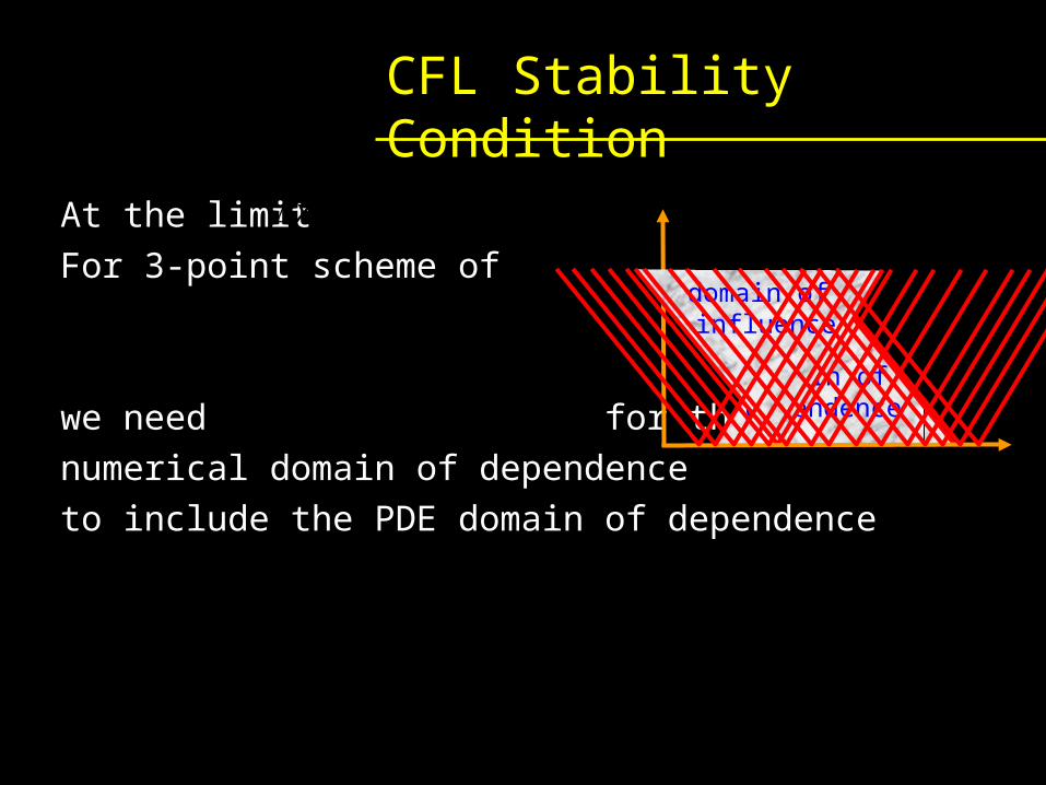
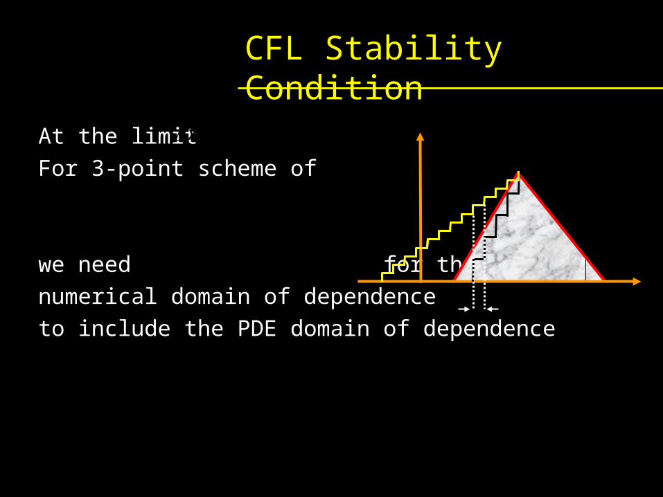
CFL Stability Condition
At the limitFor 3-point scheme of
we need for the numerical domain of dependenceto include the PDE domain of dependence
0)( xt uHu
0 0, tx t
x1x
tx ~,~
domain of dependence
0x
domain of influence
x̂
'1 Hx
t
CFL Stability Condition
At the limitFor 3-point scheme of
we need for the numerical domain of dependenceto include the PDE domain of dependence
0)( xt uHu
0 0, tx t
x1x
tx ~,~
0x
'1 Hx
t
x
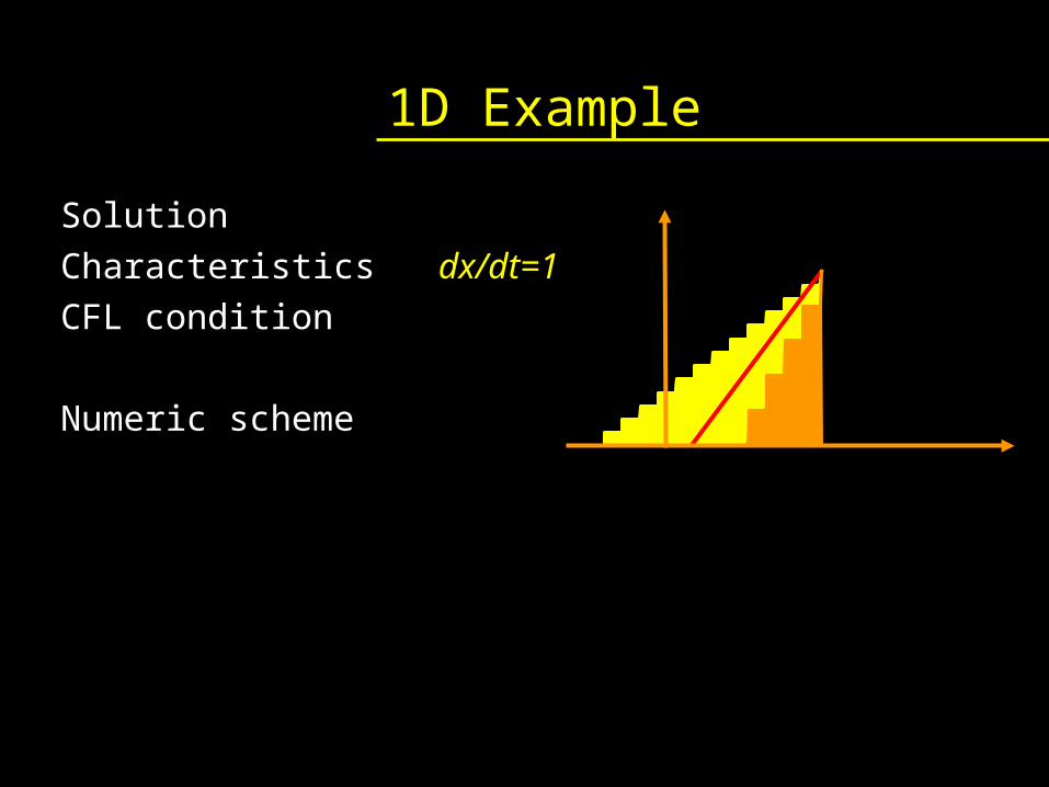
1D Example
SolutionCharacteristics dx/dt=1CFL condition
Numeric scheme
xt uu
)0,(),( txutxu t
x
tx 0
0x
x
t
1
ni
xni
t uDuD

1D Example
where
Characteristics
Numeric scheme
CFL condition
xt uxau )(
1 1
1 1)(
x
xxa
t
x
ta
x
)2()(
))0,min()0,(max(
112||
1121 n
ini
ni
ani
ni
axtn
ini
ni
xi
ni
xi
ni
t
uuuuuuu
uDauDauDii
1 1
1 1
x
x
dx
dt
1
xxxxi uauax ||||
Numerical viscosity
2D Example
Numeric scheme
CFL condition
t
2
1
h
t
2,1,1
12
22
)0,,min(max)0,,max(
)0,,max()0,,max(
nji
nji
nijh
nij
xnij
x
nij
ynij
ynij
xnij
xnij
t
DD
DDDDD
tt NC

2D Examples
Some flows
Vt
31
31
31 22
22
22
2div
2div
xyyyxxyyxxtt
yx
xyyyxxyyxxtt
tt
NC
NC
NC
require upwind/monotoneschemes
,2
div ,
22
22
gg
gNNggC
yx
xyyyxxyyxx
tt


![Active contours for multi-region image segmentation with a ...web.stanford.edu/~adkarni/publications/DRK_SSVM13.pdf · 2 Anastasia Dubrovina, Guy Rosman and Ron Kimmel [36,35,29]](https://img.pdfslide.net/doc/110x75/5e099e0f128dd76505178c90/active-contours-for-multi-region-image-segmentation-with-a-web-adkarnipublicationsdrkssvm13pdf.jpg)