Leveling the Playing Field?The Role of Public Campaign Funding

in Elections∗

Tilman Klumpp† Hugo M. Mialon‡ Michael A. Williams§

March 8, 2015

Abstract

In a series of First Amendment cases, the U.S. Supreme Court established that governmentmay regulate campaign finance, but not if regulation imposes costs on political speech andthe purpose of regulation is to “level the political playing field.” The Court has applied thisprinciple to limit the ways in which governments can provide public campaign funding tocandidates in elections. A notable example is the Court’s decision to strike down matchingfunds provisions of public funding programs (Arizona Free Enterprise Club’s Freedom ClubPAC v. Bennett, 2011). In this paper, we develop a contest-theoretic model of elections inwhich we analyze the effects of public campaign funding mechanisms, including a simplepublic option and a public option with matching funds, on program participation, politicalspeech, and election outcomes. We show that a public option with matching funds isequivalent to a simple public option with a lump-sum transfer equal to the maximum level offunding under the matching program; that a public option does not always “level the playingfield” but may make it more uneven and can decrease as well as increase the quantity ofpolitical speech by all candidates, depending on the maximum public funding level; and thata public option tends to increase speech in cases where it levels the playing field. Severalof the Supreme Court’s arguments in Arizona Free Enterprise are discussed in light of ourtheoretical results.

Keywords: Campaign finance; public options; clean election programs; matching funds;trigger funds; First Amendment; U.S. Supreme Court.

JEL codes: D72, H41, H71, H76, K19

∗We thank David Park for outstanding research assistance.†University of Alberta, Department of Economics. 9-20 Tory Building, Edmonton, AB, Canada T6G 2H4. E-mail:

klumpp@ualberta.ca.‡Emory University, Department of Economics. Rich Building 317, 1602 Fishburne Dr., Atlanta, GA 30322, USA.

E-mail: hmialon@emory.edu.§Competition Economics, LLC. 2000 Powell Street, Suite 510, Emeryville, CA 94608, USA. E-mail:

mwilliams@competitioneconomics.com.

1 Introduction

Half of the states in the U.S. provide some form of public funding to political campaigns in stateelections, and sixteen of these states allocate public funds directly to candidates. As a generalrule, political candidates who accept public funding are required to limit their campaign spendingand restrict their private fundraising activities.1 The goals of public campaign funding includecurbing political corruption and helping less wealthy candidates remain competitive in racesagainst well-funded opponents.

In a series of highly publicized cases, however, the U.S. Supreme Court has placed limits onthe interests that government can legitimately pursue when regulating campaign finance, includingrestrictions on the ways in which public campaign funding can be provided. In particular, theCourt has established that government may regulate campaign finance, but not if regulationimposes costs on political speech and the primary purpose of regulation is to “level the politicalplaying field.” 2 This doctrine has affected public campaign financing programs in several U.S.states. In particular, public financing programs that try to achieve a financial balance in electionsby allocating state funds to participating candidates in direct response to campaign spending bynon-participating candidates are unconstitutional, as they impose an unjustifiable burden on thespeech of the latter.

In this paper, we examine formally the effects of different public campaign financing mecha-nisms on political speech and election outcomes. To do so, we develop a contest-theoretic modelin which two candidates compete by engaging in costly political speech. The winning candidateis determined through a Tullock success function, so that the likelihood of election increases in acandidate’s own speech and decreases in the speech of the opponent. Candidates differ in theircosts of raising private funds, reflecting differences in wealth or access to wealthy donors. Wethen introduce public campaign funding to this framework. Participation in a public programfrees a candidate from the need to raise private funds, but limits his speech to the level feasiblewith public funds.

Our model encompasses a variety of public funding mechanisms. One such mechanism is asimple public option: Candidates who participate in the program receive a one-time, lump-sumtransfer of state funds to be used in their campaigns, but they are barred from raising private funds.This is the most common form of public funding used in the U.S. states. Another mechanismis a public option with matching funds (also called trigger funds). This mechanism works as

1The strongest form of these restrictions is imposed by clean elections systems, which prohibit publicly fundedcandidates from accepting any private donations. Seven states have adopted clean elections laws to datte: Arizona,Connecticut, Maine, New Jersey, New Mexico, North Carolina, and Vermont. Source: National Conference of StateLegislatures (www.ncsl.org).

2Landmark decisions that were based on the “leveling the playing field” argument include Davis v. FEC (2008),which concerns individual private campaign contribution limits; Citizens United v. FEC (2010), which concerns theregulation of independent political expenditures; Arizona Free Enterprise Club’s Freedom Club PAC v. Bennett (2011),which concerns the provision of public campaign funds and which we discuss in more detail in Section 5 of this paper;and McCutcheon v. FEC (2014), which concerns aggregate private campaign contribution limits.

1

follows: Candidates who opt for public financing first receive an initial distribution of state fundsto their campaigns. If campaign spending by privately funded candidates exceeds this initialpublic outlay, additional matching transfers are made to publicly funded candidates, up to apredetermined maximum. Until 2010, matching programs were used in a number of jurisdictions,most prominent among them Arizona and Maine. In 2011, the Supreme Court declared theseprograms unconstitutional, as matching mechanisms disburse public funds in direct response toprivate campaign spending, impermissibly burdening the speech of privately financed candidates(Arizona Free Enterprise Club’s Freedom Club PAC v. Bennett, 564 U.S. 2011, henceforth“Arizona Free Enterprise”).3

We examine both funding mechanisms in our contest model and establish a number of sur-prising, and often counterintuitive, results. These results call into question the way in which theSupreme Court has applied its “leveling the playing field” doctrine to determine the constitution-ality of public campaign funding programs. Specifically, we reach the following conclusions:

1. We show that a public option with matching funds is equivalent, in terms of the candidates’participation decicions, equilibrium election probabilities, private spending, and payoffs,to a simple public option whose lump-sum transfer equals the maximum possible fundinglevel under the matching program. Thus, the argument that the provision of matching funds,in order to level the playing field, burdens private speech would, if valid, apply equally tosimple public options. Yet, simple public options remain legal while those that include amatching mechanism do not.

2. We then examine if public funding levels the political playing field in the first place. Wedemonstrate that, when some candidates choose to participate in the public program butothers do not, privately funded candidates may be more or less likely to win than theywould be if public funding were not available to their opponents. Conversely, removing orrestricting a public financing program may lower the election probability of candidates thatdo not accept the public option. The reason is that a publicly funded candidate is constrainedby the funding maximum level permitted under the program, and thus can be outspent byan unconstrained candidate relatively easily. It is even possible that all candidates prefer theavailability of a public option over a purely private system of campaign finance, including

3Arizona and Maine enacted clean elections acts in 1998 and 1996, respectively, and used matching mechanismscomprehensively in all elections for state offices. In addition, several other states have used matching provisions as partof their public election funding programs. Minnesota operated an early matching program but was forced to abolish itin 1994 following a federal court decision (Day v. Holahan, 34 F.3d 1356, U.S. Court of Appeals, 8th Circuit, 1994).Connecticut adopted its matching program in 2006, but abolished it four years later following a separate federal courtdecision (Green Party of Connecticut v. Garfield, 616 F.3d 189, U.S. Court of Appeals, 2nd Circuit, 2010). Matchingprograms were also used in judicial elections in North Carolina and West Virginia, gubernatorial elections in Florida,as well as in municipal elections in Albuquerque, Los Angeles, and San Francisco. For detailed legal analyses ofmatching provisions in public campaign finance and the court challenges against them, see LoBiondo (2011), Hudson(2012), Rahmanpour (2012), and Steele (2012).

2

candidates who do not use the public option.4 Yet, the plight of privately funded candidateswho ran against state-funded opponents was a major concern of the Supreme Court inArizona Free Enterprise.

3. Finally, we examine how public campaign financing affects the candidates’ incentives toengage in political speech. We show that if a small increase in the funding level of a publicprogram induces additional candidates to forgo private fundraising and receive state fundsinstead, political speech decreases. However, this effect is reversed when participationdecisions do not change. In particular, we show that in any equilibrium in which onecandidate accepts a simple public option while the other elects to raise funds privately, theintroduction of additional matching funds increases speech by all candidates. We also showthat public funding systems that increase total speech are systems that level the playingfield.

In addition to casting doubt on the validity of several of the arguments the Supreme Courtmade when evaluating the effects of public campaign funding programs, our theoretical resultsalso allow us to examine the validity of empirical assessments of these effects. Some authorshave proposed the following test to determine whether a public option with matching funds chillspolitical speech: If it does, then private campaign spending should cluster just below the initialdisbursement paid to publicly funded candidates (Gierzynski 2011; Dowling et al. 2012). Electionfinance data for states that had matching programs does not reveal such clustering, suggestingthat privately funded candidates were not effectively constrained in their speech. The state ofArizona used the same argument when it defended its matching provision before the SupremeCourt. We show that the presence or absence of clustering cannot be used to infer that publicfunding affects the level of speech.

In sum, our results suggest that a number of important strategic aspects of public campaignfunding programs may have been misunderstood by courts and academics alike. The gametheoretic model that leads us to this conclusion is admittedly stylized. However, the fact thatthe predictions from even this simple model are often at odds with intuition provides all themore reason to be cautious when using intuitive reasoning to predict the effects of public fundingprograms on election outcomes, campaign spending, and political speech.

The remainder of the paper is organized as follows. In Section 2 we review the relatedliterature. In Section 3 we present a contest model of two-candidate elections with private andpublic campaign funding, and in Section 4 we derive its equilibria. In Section 5 we discussthe Supreme Court’s Arizona Free Enterprise ruling in light of our model results. In Section 6we examine the extent to which our results are robust to a number of alternative modeling

4This scenario can indeed be an equilibrium: Financially weaker candidates may prefer to accept public funding,not because of how it affects their probability of election but because of the cost savings it entails. Conversely,financially stronger candidates may prefer to run against publicly funded candidates who, because they participate inthe public program, are constrained in their private fundraising and spending activities.

3

choices. These include funding decisions that are made sequentially (instead of simultaneously),asymmetries in the canddidates’ impact of political speech (instead of their fundraising costs),and the introduction of risk in private fundraising. Section 7 concludes. Most proofs are in theAppendix.

2 Literature Review

The clean elections acts passed in Arizona and Maine in the late 1990s were the first cleanelections acts and still constitute the most comprehensive attempts at campaign finance reformin the United States to date (for an overview of earlier reforms, see Jones 1981). For thisreason, a number of studies have examined the effects of public campaign financing in bothstates. These papers investigate a very similar set of questions that we examine here: How doespublic funding affect candidates’ election probabilities; how does public funding affect campaignspending and political speech; and what are the effects (if any) of providing public funds throughmatching mechanisms instead of lump-sum. Unlike our paper, however, the previous literaturehas addressed these questions empirically.

Public campaign financing and election probabilities. Malhotra (2008) compares win margins forincumbents in senate races in Arizona and Maine before and after these states introduced a publicoption in 2000. He finds that win margins for incumbents decreased from 1998 to 2000. Stratmann(2009) finds that public financing in Maine reduced vote margins in House elections compared toother states with limited or no public financing. However, in a recent survey of the literature onthe effects of laws on public funding of elections across all states, Mayer (2013) concludes thatwhile there is some evidence that public funding may have slightly increased competitivenessin state legislative elections, mainly by reducing the number of uncontested elections, there isno evidence that it has increased competitiveness of contested elections. Moreover, there is noevidence that it has changed incumbency reelection rates or margins of victory in the longer run.The effects are even less discernable in statewide elections. Primo, Milyo, and Groseclose (2006)find no significant effect of public funding on the competitiveness of gubernatorial elections.

Public campaign financing and election spending. Miller (2011a) finds that total spending inArizona House and Senate races increased significantly after 2000, and that total spending inMaine House and Senate races decreased slightly after 2000. Miller (2011b) finds that publiclyfunded candidates in Arizona and Maine spent more time interacting with the public in crucialelection phases, compared to privately funded candidates (a possible reason being that publiclyfunded candidates need to spend less time fundraising). Miller (2012) finds that the introductionof a public option in Arizona and Maine yielded greater benefits to Democratic challengers thanto Republican ones.

Public campaign financing and matching programs. Several papers examine specifically thematching mechanisms that were part of the programs operated by Arizona and Maine. Miller

4

(2008) and U.S. Government Accountability Office (2010) examine empirically the effects ofmatching funds provisions in Arizona and Maine on the timing of privately funded candidates’expenditures. These studies find that privately funded candidates strategically delay their ex-penditures in order to postpone triggering matching funds for their publicly funded opponents.Gierzynski (2011) and Dowling et al. (2012) examine whether contributions to privately financedcandidates in state congressional elections in Maine and Arizona exhibit clustering below theinitial funding level of publicly financed candidates. Since contributions beyond this thresholdtrigger matching payments to publicly financed candidates, clustering just below the matchingthreshold might indicate that matching funds chill private speech. However, no evidence of suchclustering is found. Dowling et al. (2012) also compare the evolution of aggregate campaigncontributions in Arizona to those in Maine, as well as a synthetic control state, to estimate thetreatment effect associated with the injunction halting Arizona’s matching program in 2010. Noevidence is found that the injunction increased contributions in Arizona, relative to the comparisonstates.

Our paper contributes to this literature by providing a formal, game theoretic model that allowsus to examine the channels through which both simple public options and matching programsaffect election probabilities and campaign spending. It complements the empirical literature byproviding an analytical framework, based on contest theory, that can help explain several of theempirical findings discussed above. For example, we provide conditions under which publiccampaign funding makes elections more competitive and less competitive, and we explain whypublic funding programs that include a matching component do not result in clustered spendingby privately funded candidates.

Finally, we note for completeness that a number of authors have investigated other types ofmatching mechanisms. Coate (2004) and Ashworth (2006) theoretically analyze the properties ofcampaign finance systems in which the state matches any private contributions to a party withpublic contributions to the same party.5 These programs can provide a “continuous” alternativeto more conventional threshold grants that require candidates to demonstrate their viability bycollecting a certain amount of private donations before becoming eligible for a fixed publicsubsidy. Our paper does not analyze this type of matching mechanism. In contrast, we examine asystem that matches private contributions to a candidate with public contributions to opposingcandidates. Ortuno-Ortı́n and Schultz (2004), Prat et al. (2010), and Klumpp (2014) examineEuropean systems of public financing, in which candidates receive public funds in proportionto their vote shares. In contrast, we analyze American systems of public financing, in whichcandidates receive a lump-sum transfer of money and, possibly, matching grants that dependdirectly on contributions to their opponents, but not on election outcomes.

5Such programs are presently in use in Florida, Hawaii, Maryland, Massachusetts, Michigan, New Jersey, andRhode Island. Source: National Conference of State Legislatures (www.ncsl.org).

5

3 Election Contests with Public Campaign Funding

Two candidates (i = 1, 2) compete to win an election. Both candidates attach a value of one towinning the election, and a value of zero to losing. We model electoral competition as a speech (oradvertising) contest. Let xi ≥ 0 denote candidate i’s amount of speech (i = 1, 2). The probabilitythat candidate i wins the election is given by the Tullock contest success function:

Pi = f (xi, x−i) ≡

xi

xi + x−iif x1 + x2 > 0,

1/2 if x1 + x2 = 0.(1)

where, as usual, −i denotes i’s opponent. The success function in (1), introduced in Tullock (1980),is one of several “workhorse models” employed in the literature on contests and rent-seeking (seeKonrad 2009 for an overview).

Each unit of advertising costs one unit of money and has to be paid by the politician’scampaign. For this, the campaign needs to raise contributions, either from private sources or frompublic sources. These funding sources are modelled as follows.

Private funding. If candidate i is privately funded, he freely chooses xi. The cost of raising theseprivate funds is ci xi. The coefficient ci ∈ (0,∞) has several interpretations. It may represent i’sopportunity cost of a dollar spent on campaigning. A candidate with a low ci can be thoughtof as a “rich” politician, and a candidate with a high ci can be thought of as a “poor” politician.Alternatively, ci may represent i’s fundraising costs. A candidate with a low ci can be thought ofas a politician with access to a large number of wealthy supporters, relative to one with a high ci.Both candidates’ fundraising cost parameters, c1 and c2, are common knowledge.6

Public funding. A candidate who participates in a public program incurs no fundraising costs;however, this candidate cannot raise or spend private funds. Instead, publicly funded candidate ireceives an initial transfer T0 ≥ 0 from the state to spend on his campaign.

A participating candidate whose opponent is privately funded may receive additional transfers,which are determined as follows: Let i be the publicly funded candidate and let −i be i’s privatelyfunded opponent. For every dollar spent by −i above T0, candidate i receives one dollar from thestate, until i’s funding reaches a maximum Tmax ≥ T0. The overall funds received by the publiclyfinanced candidate are then given by the formula

xi = γ(x−i) ≡

T0 if x−i ≤ T0,

x−i if T0 < x−i < Tmax,

Tmax if x−i ≥ Tmax.

(2)

6In Section 6.3 we discuss other characteristics in which candidates could differ.

6

If both candidates are publicly funded, then both receive only the initial transfer T0.7

A public funding program is hence a pair (T0,Tmax) ∈ [0,∞)2, consisting of the minimumand maximum funding level of participating candidates. A simple public option is a programsuch that 0 < T0 = Tmax. If Tmax > T0 we say that the program has matching funds. A program0 = T0 < Tmax has only matching funds, and the program (0, 0) is equivalent to there being nopublic campaign funding.

The timing of the game is as follows. First, both candidates simultaneously decide whether toparticipate in the public funding program or not (stage 1). For candidate i = 1, 2, this choice isdenoted si ∈ {Pr, Pu}. The candidates then observe each other’s choice and engage in the electoralcontest (stage 2). A publicly funded candidate does not have any further decisions to make, as hisspending level is determined automatically via (2). A privately funded candidate, on the otherhand, has to decide how much to spend.

We will investigate the subgame perfect equilibria of the game described above. These can befound as follows. Let vi(·|si, s−i) be candidate i’s payoff function in the electoral contest at stage2, given the funding choices si and s−i. This payoff function is

vi( xi, x−i | si, s−i ) =

f (xi, x−i) − cixi if (si, s−i) = (Pr, Pr),

f (xi, γ(xi)) − cixi if (si, s−i) = (Pr, Pu),

f (γ(x−i), x−i) if (si, s−i) = (Pu, Pr),

f (T0,T0) if (si, s−i) = (Pu, Pu).

(3)

Let v∗i (s1, s2) be candidate i’s expected Nash equilibrium payoff in the subgame at (s1, s2). At theinitial stage 1 of our model, a pure strategy Nash equilibrium in funding choices is then a pair(s∗1, s

∗2) ∈ {Pu, Pr} × {Pu, Pr} such that

v∗i (s∗i , s∗−i) ≥ v∗i (si, s∗−i) for i = 1, 2 and si = Pu, Pr.

In the next section, we find the subgame perfect equilibria by first computing the second-stagepayoffs v∗1 and v∗2 and then finding a stage-1 equilibrium in funding choices (s∗1, s

∗2).

Before we go on, let us note that for the purpose of this paper we equate political speech,advertising, campaign spending, and campaign fundraising. Each of these assumed equivalences

7The actual matching programs that were used in Arizona and Maine did not match dollar-for-dollar but, instead,contained small reductions in the matching rate that were meant to offset private fundraising expenses. For example,Arizona’s 2008 funding formula awarded to every participant who ran as a candidate for state representative in districtd the amount

γ(xd) = $21, 479 + min{

0.94 ·max{0, xd − $21, 479

}, $64, 437

},

where xd denotes the maximum private spending among the candidates in district d. Furthermore, both the matchingrate of 94 cents per dollar and the maximum public funding level $64, 437 could be adjusted by the state electioncommission at various points during an election cycle, depending on the proportion of Arizona’s budgeted publiccampaign funds that had already been allocated. We abstract from these details here.

7

is a simplification. First, some forms of political speech do not require much in the way of costlyadvertising (e.g., a politician giving a media interview), and we ignore such types of “non-costly”speech in our model. Second, campaigns routinely spend money they have raised on activitiesother than advertising (e.g., staff salaries, office rent, travel, or voter mobilization). Our model alsodoes not distinguish these non-advertising expenses as a separate spending category. However,to the extent that they support the communication of the candidate’s message, or increase thecandidate’s chance of success in some other way, they fit the formal structure of our contestmodel. Third, campaigns sometimes raise more money than they spend (allowing a politicianto save resources for a future election), and sometimes they spend more money than they raise(in which case the campaign must repay its debt after the election). Because ours is a static,one-shot model, we do not consider these possibilities. Instead, we assume that a campaignspends precisely as much money as it raises. These simplifications allow us to focus on the issuesraised by the Supreme Court when it evaluated public campaign funding programs in light of theFirst Amendment.

4 Equilibrium Characterization

In this section we characterize the equilibrium funding choices of the candidates, their advertisinglevels, their success probabilities, and their payoffs. In the spirit of backward induction, we firstsolve the second-stage contest conditional on the candidates’ funding choices, and then use theseresults to determine the equilibrium funding choices at the first stage.

4.1 Analysis of the second-stage contest

Consider a public campaign funding program (T0,Tmax). Suppose each candidate has made hisdecision of whether to participate in this program or not. The following three cases can then ariseat the second stage of the game.

First, if both candidates are publicly funded the outcome is trivial. Both candidates receivefrom the state the transfer T0, which they spend in the contest at no personal cost to themselves.Therefore, we have x1 = x2 = T0 and P1 = P2 = 1/2, and the candidates’ payoffs in this subgameare

v∗1(Pu, Pu) = v∗2(Pu, Pu) =12.

Next, if both candidates are privately funded, stage 2 of our model becomes a standard Tullockcontest with common prize 1 and marginal costs c1 and c2. This contest has a well-known, uniquepure strategy Nash equilibrium, in which spending levels and success probabilities are

x1 =c2

(c1 + c2)2 , x2 =c1

(c1 + c2)2 and P1 =c2

c1 + c2, P2 =

c1

c1 + c2.

8

The payoffs in this equilibrium are given by

v∗1(Pr, Pr) =(c2)2

(c1 + c2)2 , v∗2(Pr, Pr) =(c1)2

(c1 + c2)2 .

For details on the computation, we refer the reader to the large literature on Tullock contests (see,for example, Konrad 2009).

Finally, consider the case where one candidate is privately funded and the other is publiclyfunded. Without loss of generality, assume that candidate 1 is privately funded and candidate 2 ispublicly funded (the analysis is similar when the roles are reversed). Candidate 1’s payoff whenspending x1 against his opponent in the public funding system (T0,Tmax) is

x1

x1 + γ(x1)− c1x1 =

x1

x1 + T0− c1x1 if x1 ≤ T0,

1/2 − c1x1 if T0 < x1 < Tmax,

x1

x1 + Tmax− c1x1 if x1 ≥ Tmax.

(4)

Note that, in case of a simple public option, only the first line on the right-hand side of (4) isrelevant. Maximizing this payoff function with respect to x1, we get

x1 =

0 if c1 >1

T0,

√T0/c1 − T0 if 1

T0≥ c1 >

14T0,

T0 if 14T0≥ c1 >

14Tmax

,√

Tmax/c1 − Tmax if c1 ≤1

4Tmax.

(5)

(Again, in case of a simple public option, the two middle cases in (5) collapse into one.) Themoney received by publicly funded candidate 2 is now determined by using (5) in the fundingformula (2):

x2 = γ(x1) =

T0 if c1 >1

4Tmax,

Tmax if c1 ≤1

4Tmax.

(6)

Plugging both (5) and (6) into the Tullock success function, we get the following successprobabilities for candidate 1:

P1 = f (x1, x2) =

0 if c1 >1

T0,

1 −√

c1T0 if 1T0≥ c1 >

14T0,

1/2 if 14T0≥ c1 >

14Tmax

,

1 −√

c1Tmax if c1 ≤1

4Tmax.

(7)

9

Candidate 2’s success probability is then P2 = 1 − P1, and because candidate 2 has no campaigncosts his payoff is also P2. Candidate 1’s payoff is his election probability, P1, minus his privatecost, x1c1. After a few manipulations, this payoff can be written as

v∗1(Pr, Pu) =

0 if c1 >1

T0,(

1−√

c1T0)2

if 1T0≥ c1 >

14T0,

1/2 − c1T0 if 14T0≥ c1 >

14Tmax

,(1−√

c1Tmax)2

if c1 ≤1

4Tmax.

(8)

4.2 Analysis of the first-stage funding choices

The second-stage continuation payoffs v∗1(s1, s2) and v∗2(s1, s2) that we derived in Section 4.1define a normal form game that describes the initial stage of our game, at which candidates choosewhether or not to participate in the public campaign funding program (i.e., they choose s1 and s2).In an overall subgame perfect equilibrium of our model, the stage-1 funding choices must form aNash equilibrium. We distinguish three types of pure strategy equilibrium:

– All-public equilibrium: Both candidates accept the public option, i.e., (s1, s2)= (Pu, Pu).

– All-private equilibrium: Both candidates choose private funding, i.e., (s1 s2)= (Pr, Pr).

– Private-public equilibrium: One candidate chooses private funding while the other choosespublic funding, i.e., (s1, s2)= (Pr, Pu) or (s1, s2)= (Pu, Pr).

Depending on the parameters of the model—that is, the fundraising costs c1 and c2 and thepolicy parameters T0 and Tmax—all three equilibrium types can emerge:

Proposition 1. The following characterizes all pure strategy equilibria of the model. Define

K ≡3/2 −

√2

Tmax, L(c) ≡ c ·

((c Tmax)−1/4 − 1

). (9)

(a) An all-public equilibrium exists if and only if ci ≥ K (i = 1, 2). In this equilibrium, bothcandidates spend T0 from state funds and both win with probability 1/2.

(b) An all-private equilibrium exists if and only if ci ≤ L(c−i) (i = 1, 2). In this equilibrium,candidate i spends c−i/(c1+ c2)2 from private funds and wins with probability c−i/(c1+ c2).

(c) A private-public equilibrium in which candidate i is privately funded and candidate −iaccepts the public option exists if and only if ci ≤ K and c−i ≥ L(ci). In this equilibrium,candidate i spends

√Tmax/ci − Tmax from private funds and candidate −i spends Tmax from

public funds. Privately funded candidate i wins with probability 1 −√

ciTmax, and publiclyfunded candidate −i wins with probability

√ciTmax.

10

c2

c1

K

K

L(c1)

L(c2)

Pr, Pr

Pu, Pu

Pu, Pr

Pr, Pu

Pr, PuPu, Pr

Figure 1: Equilibrium funding choices for different c1, c2-combinations.

Figure 1 depicts the parameter regions that give rise to the equilibria identified in Proposition 1.If both candidates have relatively high fundraising costs, they both accept the public option (thetop right corner of the figure). If both have relatively low costs, they both reject the publicoption (the lense-shaped region in the bottom left corner). If the candidates’ fundraising costsare sufficiently asymmetric, the high-cost candidate chooses public financing while the low-costcandidate remains privately funded. In the blue-shaded region, candidate 1 choses the publicoption; and in the red-shaded region, candidate 2 chooses the public option.

In the small diamond-shaped area at the center of the figure, depicted in purple, two typesof private-public equilibrium exist—one in which candidate 1 accepts the public option but notcandidate 2, and one in which the roles are reversed. In this area, which is characterized bythe inequality L(c−i) < ci < K (i = 1, 2), the candidates’ first-stage problem constitutes ananti-coordination game (a game of “Chicken”). This implies that there is also a mixed strategyequilibrium in which candidates randomize over public and private financing.8

8In general, a Nash equilibrium (in pure or mixed strategies) is a pair (p1, p2) ∈ [0, 1] × [0, 1], where pi is theprobability that candidate i participates in the public program, such that pi > 0 (pi < 1) implies

p−ivi(Pu, Pu) + (1 − p−i)v∗i (Pu, Pr) ≥ (≤) p−ivi(Pr, Pu) + (1 − p−i)v∗i (Pr, Pr) (i = 1, 2).

11

5 Putting the Model to Use: A Rebuttal to Arizona Free Enterprise

In Arizona Free Enterprise, the Supreme Court ruled that the clean election program operated bythe state of Arizona prior to 2010, whose central component was a public option with matchingfunds, was unconstitutional. The Court’s decision was based on the following line of reasoning:

1. Public options with matching grants burden political speech in ways simple public optionsdo not.

2. The purpose of imposing this burden is to “level the political playing field,” which is not acompelling state interest in regulating speech.

3. The effect of a more level playing field is a decrease in the political speech of at least somecandidate.

The equilibria we characterized in the previous section have interesting properties that beardirectly on each of these arguments. We consider them in turn to assess the validity of the Court’sreasoning within the context of our model. In Section 5.1 we examine whether there is a materialdifference between simple public options and matching programs; in Section 5.2 we examinewhether public campaign funding (with and without matching funds) levels the political playingfield; and in Section 5.3 we examine whether a more level playing field chills political speech.

5.1 Are matching grants and simple options really different?

The Supreme Court’s central concern in Arizona Free Enterprise was not the public funding ofcandidates per se, but the matching mechanism through which the state allocated public fundsto candidates. In particular, the Court suggested that even a large lump-sum transfer from thestate to candidates may be constitutional because it does not depend on the political speech of anyprivately financed candidates:

The State correctly asserts that the candidates and independent expenditure groups“do not [. . . ] claim that a single lump sum payment to publicly funded candidates,”equivalent to the maximum amount of state financing that a candidate can obtainthrough matching funds, would impermissibly burden their speech. . . . The Statereasons that if providing all the money up front would not burden speech, providingit piecemeal does not do so either. And the State further argues that such incrementaladministration is necessary to ensure that public funding is not under- or over-distributed. . . . These arguments miss the point. It is not the amount of funding that

If a mixed strategy equilibrium exists, the probability that candidate i chooses the public option can be shown to be

pi =

(√ciTmax −

c2i

(c1 + c2)2

) / (√ciTmax −

c2i

(c1 + c2)2 +(1−

√c−iTmax

)2−

12

).

We will not consider the possibility of mixed strategy equilibrium in the rest of our analysis.

12

the State provides to publicly financed candidates that is constitutionally problematicin this case. It is the manner in which that funding is provided — in direct responseto the political speech of privately financed candidates and independent expendituregroups. (564 U.S. 2011, at 21.)

We now examine if this distinction between lump-sum transfers and matching grants is of anyconsequence in our model. Proposition 1 shows that the candidates’ incentives to select public orprivate financing depends on the public funding program (T0,Tmax) only through the maximallevel of state funding Tmax, but not on T0. Moreover, in every equilibrium the candidates’ electionprobabilities depend on Tmax only, and the same is true for the fundraising and spending of privatecandidates. Hence, we have the following:

Corollary 1. Financing decisions, election probabilities, private spending, and the candidates’payoffs under any funding program (T0,Tmax) that includes matching funds are the same as thoseunder an alternative program (Tmax,Tmax) that consists only of a simple public option in theamount Tmax but no matching funds.

The intuition behind Corollary 1 is simple. Public programs with the same maximum fundinglevel Tmax result in different outcomes only when candidates who reject public funding spend lessthan Tmax. But a candidate should not reject state funding unless he is prepared to spend more thanTmax: Spending less than Tmax from private funds against a publicly funded opponent is costlyand results in a probability of election that is at most one-half. Choosing public funding againstthe same opponent, on the other hand, entails no costs and guarantees an election probability ofone-half. Thus, a case in which the election probability of a privately funded candidate undera matching program (T0,Tmax) is different from that under a simple public option of value Tmax

cannot arise in equilibrium.9

Note that Corollary 1 does not say that removing a matching component from a publicprogram will not change election outcomes or speech. What it says is that any public fundingprogram that includes a matching component is equivalent—in terms of program participation,election outcomes, and private speech—to a simple public option whose value is equal to themaximal state funding level under the matching program. An implication of this result is thatstates can undo restrictions on matching programs imposed by courts by adopting an appropriatelychosen simple public option that replicates the equilibrium outcomes under the matching program.For example, this is how Connecticut adjusted its public funding program for gubernatorialelections when its matching funds provision was ruled unconstitutional by a federal court in 2010(Thomas 2010).

9We will return to this dominance argument again at the end of Section 5.3, where we find that the Court appliedit correctly when it rejected empirical evidence presented by Arizona in defense of its matching program, and inSection 6.1, where we examine its robustness to fundraising uncertainty as well as alternative candidate payoff

functions.

13

Moreover, Proposition 1 implies that this adjustment also leaves public campaign spendingunchanged except when all candidates choose public funding, in which case public spending ishigher in program (Tmax,Tmax) than in program (T0,Tmax). Therefore, on expectation, a matchingprogram costs the state less to operate than a simple option that results in the same participationincentives, the same amount of privately funded speech, and the same election outcomes.10 Notethat states that operated a matching program (T0,Tmax) and do not have the resources to offerthe public option (Tmax,Tmax) could respond by replacing their matching program with a simplepublic option (T,T ), where T0 < T < Tmax. In this case, the candidates’ participation decisionsas well as their speech may be affected. In particular, a candidate who would have acceptedthe public option in programs (T0,Tmax) and (Tmax,Tmax) may decline it in program (T,T ). InProposition 4 in Section 5.3 below we show that, if candidates adjust their participation decisionand the change in the program funding level is not too drastic, both candidates’ speech increases(while the cost to the state decreases).

It follows that, in our model, a matching program does not impose a burden on private politicalspeech that would not be the same in a program that consisted only of an “equilibrium-equivalent”simple public option. (In fact, the burden imposed by a simple public option could even bemore severe, as we will argue in Section 6.1.) Thus, if public options with matching funds areunconstitutional because they burden the speech of privately funded candidates or independentexpenditure groups, then the same must be true for simple options.

5.2 Does public campaign funding level the political playing field?

In a series of First Amendment cases, the U.S. Supreme Court has ruled that burdens on politicalspeech that are imposed to achieve a balance of speech between candidates are unconstitutional(see Footnote 3). The decision in Arizona Free Enterprise follows the same doctrine:

We have repeatedly rejected the argument that the government has a compelling stateinterest in “leveling the playing field” that can justify undue burdens on politicalspeech. . . . [I]n a democracy, campaigning for office is not a game. It is a criticallyimportant form of speech. The First Amendment embodies our choice as a Nationthat, when it comes to such speech, the guiding principle is freedom—the “unfetteredinterchange of ideas”—not whatever the State may view as fair. (564 U.S. 2011,at 24–25.)

In the preceding section, we compared public financing programs that include matching grantsand those that consist only of a simple option equal to the maximum funding level under thematching program. We showed that both result in the same relative speech by each candidate, andhence in the same election probabilities. Put differently, in our model matching grants and simple

10The same argument was made by Judge Elena Kagan in her dissent to Arizona Free Enterprise. See 564 U.S.2011, Kagan, J., dissenting, at 9.

14

options alter the balance of political speech in the same way, compared to a hypothetical scenarioin which no public funding is available. Thus, if matching programs are unconstitutional becausestates may use them to “level the playing field,” the same must be true for simple public options.

The Court’s reasoning when it declared matching funds unconstitutional is based on theassumption that a public option with matching funds does, indeed, “level the playing field,” anddoes so at the expense of burdening political speech. In this section, we examine how publicfunding programs—with or without matching funds—affect the balance of political speech,showing that it can increase as well as decrease balance. In the following section, we examinehow it affects the quantity of speech, showing that it can increase as well as decrease speech,and that it tends to increase speech in cases where it “levels the playing field.” To do so, wecompare our model equilibria under a public financing program to those of a counterfactualcontest in which no public funding is available. The equilibrium of this counterfactual contestwill necessarily be of the all-private type. As shown in Section 4.1, in an all-private equilibriumthe candidate with the larger fundraising cost (the disadvantaged candidate) is outspent by thecandidate with the lower fundraising cost (the advantaged candidate) and is less likely to winagainst this opponent. Compared to this case, a public financing program can have five possibleeffects on relative spending and election probabilities:

– It unlevels the playing field if the disadvantaged candidate’s equilibrium funding share andelection probability is less than it would be without the program;

– it leaves the playing field unchanged if the disadvantaged candidate’s equilibrium fundingshare and election probability is the same as it would be without the program;

– it partially levels the playing field if the disadvantaged candidate’s equilibrium fundingshare and election probability is greater than it would be without the program, but less than1/2;

– it fully levels the playing field if the disadvantaged candidate’s equilibrium funding shareand election probability is equal to 1/2;

– it reverses the playing field if the disadvantaged candidate’s equilibrium funding share andelection probability is greater than 1/2.

All five possibilities can arise in our model, and the following result provides a completecharacterization of the possible effects of public financing on the political playing field, assumingcandidates play pure strategy equilibria.

15

Proposition 2. Suppose that candidate i is the advantaged candidate (i.e., ci < c−i). The effectsof public funding program (T0,Tmax) in pure strategy equilibrium are the following:

(a) The program unlevels the playing field if and only if(ci

c1 + c2

)2 ci

(c1 + c2)2 ≤ Tmax < min

ci

(c1 + c2)2 ,3/2 −

√2

ci

.(b) The program leaves the playing field unchanged if and only if

Tmax ≤

(ci

c1 + c2

)2 ci

(c1 + c2)2 .

(c) The program partially levels the playing field if and only if

ci

(c1 + c2)2 < Tmax ≤3/2 −

√2

ci.

(d) The program fully levels the playing field if and only if

Tmax ≥3/2 −

√2

ci.

(e) The program reverses the playing field if and only if(c−i

c1 + c2

)2 c−i

(c1 + c2)2 ≤ Tmax ≤3/2 −

√2

c−i.

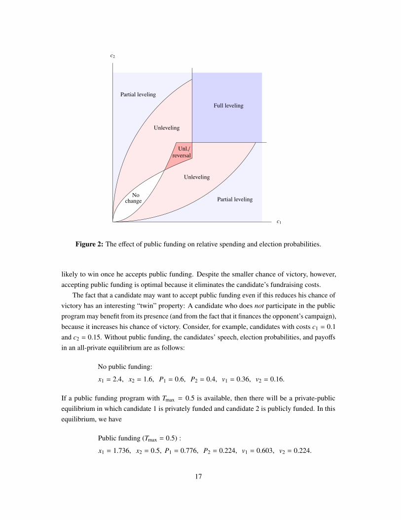
All five cases in Proposition 2 depend on the candidates’ costs in relation to the maximumpublic funding level Tmax, but not on T0 (showing again that it does not matter if Tmax is distributedas a lump-sum payment or through a matching mechanism). Figure 2 depicts these cases fordifferent (c1, c2)-pairs, holding Tmax fixed.

The ‘full leveling’ (dark blue) and ‘no change’ (white) regions correspond precisley to theall-public and all-private regions in Figure 1. The private-public region is divided into a part wherefundraising costs are relatively asymmetric, resulting in a partial leveling of the playing field(light blue); and a part where fundraising costs are relatively symmetric, resulting in an unlevelingof the playing field (light red). The possibility of a reversed playing field arises in the small centerregion where our model gave rise to two private-public equilibria (dark red). A reversal occurs inthe equilibrium in which the candidate with the higher cost rejects public financing, while thecandidate with the lower cost accepts it. In this case, the advantaged candidate would have beenmore likely to win than his opponent if both were forced to raise private funds, but becomes less

16

c2

c1

Nochange

Full leveling

Partial leveling

Partial leveling

Unleveling

Unleveling

Unl./reversal

Figure 2: The effect of public funding on relative spending and election probabilities.

likely to win once he accepts public funding. Despite the smaller chance of victory, however,accepting public funding is optimal because it eliminates the candidate’s fundraising costs.

The fact that a candidate may want to accept public funding even if this reduces his chance ofvictory has an interesting “twin” property: A candidate who does not participate in the publicprogram may benefit from its presence (and from the fact that it finances the opponent’s campaign),because it increases his chance of victory. Consider, for example, candidates with costs c1 = 0.1and c2 = 0.15. Without public funding, the candidates’ speech, election probabilities, and payoffsin an all-private equilibrium are as follows:

No public funding:

x1 = 2.4, x2 = 1.6, P1 = 0.6, P2 = 0.4, v1 = 0.36, v2 = 0.16.

If a public funding program with Tmax = 0.5 is available, then there will be a private-publicequilibrium in which candidate 1 is privately funded and candidate 2 is publicly funded. In thisequilibrium, we have

Public funding (Tmax = 0.5) :

x1 = 1.736, x2 = 0.5, P1 = 0.776, P2 = 0.224, v1 = 0.603, v2 = 0.224.

17

Here, public financing unlevels the playing field and at the same time decreases the absluteamount of speech by each candidate. Both effects help the privately funded candidate, who isnow more likely to win with less effort. The disadvantaged candidate is less likely to win, butprefers this outcome all the same because of the cost-savings he enjoys by not having to raiseprivate funds. In this example, the availability of public funding is a Pareto improvement for thecandidates even though only one of them accepts public funding.11

We conclude that, while states that institute public financing programs may or may not do sowith the intention of leveling the political playing field, the ex post impact of such programs canbe anything—from a leveling effect, to the opposite, to nothing at all—depending on the privatefundraising costs of the candidates. Without further information as to the relative likelihood ofthe cases listed in Proposition 2, the actual consequences of any given program for the balance ofspeech are impossible to assess.12

5.3 Does public campaign funding chill political speech?

Campaign finance regulations and the First Amendment are inherently at odds—the latter guar-antees private entities to be free from government-imposed burdens on their speech, while theformer imposes implicit costs on the most important form of speech, that is, political speech. Ofinterest in campaign finance cases, therefore, is the question of whether these costs are so highthat they reduce the speech of some, or all, candidates in an election. In Arizona Free Enter-prise, the Supreme Court concluded that the burden imposed by Arizona’s matching program onnon-participating candidates was sufficiently severe:

Any increase in speech resulting from the Arizona law is of one kind and onekind only—that of publicly financed candidates. The burden imposed on privately fi-nanced candidates and independent expenditure groups reduces their speech. . . . Thus,even if the matching funds provision did result in more speech by publicly financedcandidates and more speech in general, it would do so at the expense of impermissi-bly burdening (and thus reducing) the speech of privately financed candidates andindependent expenditure groups.13 (564 U.S. 2011, at 15.)

11If society values an “unfettered interchange of ideas,” the fact that the program decreased speech by bothcandidates could be considered a negative externality. We will examine the effect of public funding on the absoluteamount of speech in Section 5.3.

12One could argue that states that want to level the political playing field would only institute a public policy to thiseffect if the playing field is rather uneven to begin with, and Figure 2 suggests that, in such a case, public campaignfinancing often achieves at least a partial balancing of speech. But even if this is so, the public funding programwould achieve its goal regardless of whether it contains a matching funds provision or only a (large enough) lump-sumtransfer.

13The Supreme Court actually went further than that. While it believed that a decrease in privately funded speechwas an undesirable consequence of Arizona’s matching provision, it made clear that a burden on an activity remains aburden even when it does not decrease the activity (564 U.S. 2011, at 19). Thus, it is possible that the Court wouldhave ruled the matching program unconstitutional even if it did not have speech-chilling effects.

18

We now examine the validity of this claim within the context of our theoretical model. To doso, we derive its comparative statics and examine the effects of changes in the policy parametersT0 and Tmax on the equilibrium. The effect of matching funds on speech is then the derivative ofequilibrium advertising with respect to Tmax.

Let us first consider the case where a change in the policy parameters does not affect thecandidates’ decisions to participate in the public program. That is, any adjustments in x1 and x2

are on the “intensive margin.” The following result determines the direction of these adjustmentsfor the three types of equilibrium we characterized previously:

Proposition 3. Suppose that either T0 or Tmax increases, without altering the candidates’ equi-librium funding choices.

(a) In an all-private equilibrium, speech by each candidate remains unchanged.

(b) In an all-public equilibrium, speech by each candidate either remains constant (if only Tmax

increases but T0 is constant) or increases strictly (if T0 increases).

(c) In a private-public equilibrium, speech by each candidate either remains constant (if onlyT0 increases but Tmax is constant) or increases strictly (if Tmax increases).

Part is (c) speaks directly to the scenario the Supreme Court alluded to in the quote above,namely, a privately financed candidate running against a publicly financed candidate. In this case,a small increase in Tmax increases the speech of both candidates, while a small decrease in T0

does not decrease it. Because this applies, inter alia, to the case Tmax = T0, we have the followingresult:

Corollary 3. Suppose the public funding program consists of a simple public option. Considerany equilibrium in which one candidate accepts this option and the other candidate rejects it.Then the introduction of a small additional amount of funds, awarded through matching, resultsin a strict increase of both candidates’ speech. Conversely, awarding some of the existing amountof the public option through matching instead of lump-sum, does not decrease speech by eithercandidate.

The reason why not only the publicly funded candidate, but also the privately funded candidate,increases his speech when additional matching funds become available is the following. In atwo-player Tullock contest model, as is ours, strategies are strategic complements for the playerwho spends the larger amount. In a private-public equilibrium, this is the player who is privatelyfunded (see our discussion in Section 5.1). Adding matching funds to a public option thereforeallows the publicly funded candidate to increase his speech, and because his opponent views hisown spending and that of the publicly funded candidate as strategic complements, he increaseshis speech as well.

Next, consider the case where a change in the public funding program affects the candidates’financing choices; for example, a privately funded candidate decides to switch to the public

19

program. The resulting changes in x1 and x2 are then “extensive margin” adjustments. In ArizonaFree Enterprise the Supreme Court was also concerned with the potentially speech-reducingeffects of such adjustments:

If the matching funds provision achieves its professed goal and causes candidatesto switch to public financing . . . there will be less speech: no spending above theinitial state-set amount by formerly privately financed candidates, and no associatedmatching funds for anyone. Not only that, the level of speech will depend on theState’s judgment of the desirable amount, an amount tethered to available (and oftenscarce) state resources. (564 U.S. 2011, at 15.)

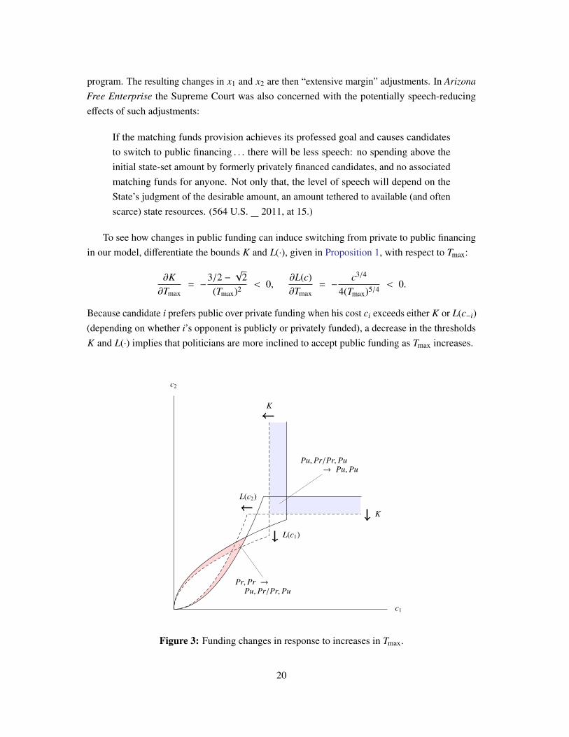
To see how changes in public funding can induce switching from private to public financingin our model, differentiate the bounds K and L(·), given in Proposition 1, with respect to Tmax:

∂K∂Tmax

= −3/2 −

√2

(Tmax)2 < 0,∂L(c)∂Tmax

= −c3/4

4(Tmax)5/4 < 0.

Because candidate i prefers public over private funding when his cost ci exceeds either K or L(c−i)(depending on whether i’s opponent is publicly or privately funded), a decrease in the thresholdsK and L(·) implies that politicians are more inclined to accept public funding as Tmax increases.

c2

c1

K

K

L(c1)

L(c2)

Pu, Pr/Pr, Pu→ Pu, Pu

Pr, Pr →Pu, Pr/Pr, Pu

Figure 3: Funding changes in response to increases in Tmax.

20

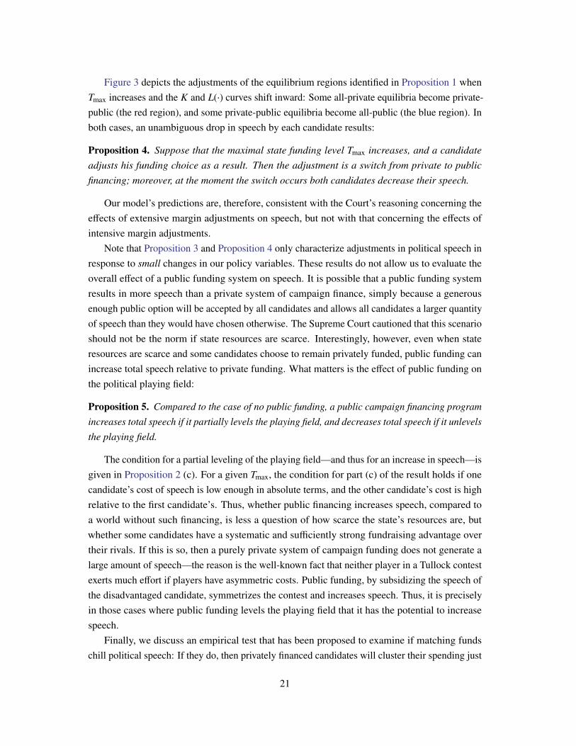
Figure 3 depicts the adjustments of the equilibrium regions identified in Proposition 1 whenTmax increases and the K and L(·) curves shift inward: Some all-private equilibria become private-public (the red region), and some private-public equilibria become all-public (the blue region). Inboth cases, an unambiguous drop in speech by each candidate results:

Proposition 4. Suppose that the maximal state funding level Tmax increases, and a candidateadjusts his funding choice as a result. Then the adjustment is a switch from private to publicfinancing; moreover, at the moment the switch occurs both candidates decrease their speech.

Our model’s predictions are, therefore, consistent with the Court’s reasoning concerning theeffects of extensive margin adjustments on speech, but not with that concerning the effects ofintensive margin adjustments.

Note that Proposition 3 and Proposition 4 only characterize adjustments in political speech inresponse to small changes in our policy variables. These results do not allow us to evaluate theoverall effect of a public funding system on speech. It is possible that a public funding systemresults in more speech than a private system of campaign finance, simply because a generousenough public option will be accepted by all candidates and allows all candidates a larger quantityof speech than they would have chosen otherwise. The Supreme Court cautioned that this scenarioshould not be the norm if state resources are scarce. Interestingly, however, even when stateresources are scarce and some candidates choose to remain privately funded, public funding canincrease total speech relative to private funding. What matters is the effect of public funding onthe political playing field:

Proposition 5. Compared to the case of no public funding, a public campaign financing programincreases total speech if it partially levels the playing field, and decreases total speech if it unlevelsthe playing field.

The condition for a partial leveling of the playing field—and thus for an increase in speech—isgiven in Proposition 2 (c). For a given Tmax, the condition for part (c) of the result holds if onecandidate’s cost of speech is low enough in absolute terms, and the other candidate’s cost is highrelative to the first candidate’s. Thus, whether public financing increases speech, compared toa world without such financing, is less a question of how scarce the state’s resources are, butwhether some candidates have a systematic and sufficiently strong fundraising advantage overtheir rivals. If this is so, then a purely private system of campaign funding does not generate alarge amount of speech—the reason is the well-known fact that neither player in a Tullock contestexerts much effort if players have asymmetric costs. Public funding, by subsidizing the speech ofthe disadvantaged candidate, symmetrizes the contest and increases speech. Thus, it is preciselyin those cases where public funding levels the playing field that it has the potential to increasespeech.

Finally, we discuss an empirical test that has been proposed to examine if matching fundschill political speech: If they do, then privately financed candidates will cluster their spending just

21

below the initial public grant T0, as, at this threshold, the marginal benefit of a campaign dollarspent against a publicly financed candidate is neutralized by the state’s matching transfers. Theabsence of clustering in actual campaign finance data from Maine and Arizona has been cited asevidence that these states’ matching programs did not reduce privately financed speech in boththe academic literature (see Gierzynski 2011; Dowling et al. 2012) and in the arguments the stateof Arizona brought before the Supreme Court in defense of its matching funds program.

In our model, it is indeed true that the marginal benefit of private spending against a publiclyfunded opponent is zero when private spending equals T0, while the marginal cost is positive(see Equation (4), assuming Tmax > T0). But, as we argued earlier, spending less than T0 fromprivate funds against a publicly financed opponent is dominated by choosing the public option.The Supreme Court rejected the empirical “evidence” for the same reason:

The State contends that if the matching funds provision truly burdened the speechof privately financed candidates and independent expenditure groups, spending onbehalf of privately financed candidates would cluster just below the triggering level,but no such phenomenon has been observed. . . . That should come as no surprise.The hypothesis presupposes a privately funded candidate who would spend his ownmoney just up to the matching funds threshold, when he could have simply takenmatching funds in the first place. (564 U.S. 2011, at 19.)

We point out, however, that the reasoning should be independent of whether the state operatesa matching program or offers only a simple public option: By Proposition 1 (c), the equilibriumspeech by a privately financed candidate who runs against a publicly financed candidate is√

Tmax/ci − Tmax ≥√

Tmax/K − Tmax = Tmax ·((

3/2−√

2)−1/2

− 1)> Tmax ≥ T0.

Thus, while public options or matching funds may or may not reduce speech, the absence ofprivate spending clustered at T0 is not evidence for or against either of these possibilities.

6 Robustness and Extensions

In this section, we introduce several alternatives to our model assumptions and discuss if, andhow, our model predictions would change under these alternatives. In Section 6.1 we revisitthe equivalence of simple public options and matching mechanisms when private fundraising isrisky, or when candidates’ funding decisions are motivated by ideological, instead of monetary,considerations. In Section 6.2 we extend our model to allow candidates to condition their fundingchoice on their opponent’s choice. In Section 6.3 we change our model so that candidates differin the impact of their speech, instead of their fundraising costs.

22

6.1 Uncertain fundraising costs and ideologically motivated candidates

We argued that awarding public campaign funds through a matching mechanism, or througha simple public option in the amount equal to the maximum funding level under the matchingprogram, does not affect the candidates’ participation decisions, their election probabilities, ortheir payoffs. The reason is that any candidate who spends less than the state maximum Tmax

from private funds would be better off if he accepted public financing. But if privately financedcandidates always spend more than Tmax, a publicly funded opponent of a privately fundedcandidate will have resources Tmax regardless of the mechanism through which Tmax is paid. Thus,a privately funded candidate is not worse off if the state awards some of Tmax through a matchingprogram instead of awarding all of Tmax in a lump-sum fashion.

Several counterarguments could be made to dismiss the above reasoning. First, a candidatesmay decline to participate in the public funding program in the expectation that he will raiseprivate funds in excess of the state maximum Tmax. If this candidate’s fundraising cost turns outhigher than anticipated, he might adjust his fundraising and spending by an amount that dependson whether the public funding program is lump-sum or has a matching component.

Consider the following example. The public program is (T0,Tmax) = (1, 2) and the candidateshave made funding decisions (s1, s2) = (Pr, Pu). These decisions would arise in equilibriumif c1 < K = 0.0428 and c2 > L(c1). Suppose that, after having declined public funding,candidate 2 learns that, unexpectedly, his fundraising cost has increased to c1 = 0.15. Since1/(4T0) > c1 > 1/(4Tmax) now, using (5)–(6) we have

x1 = 1.00, x2 = 1.00, x1 + x2 = 2.00.

That is, candidate 1 spends exactly the state minimum, as any additional campaign dollar up toTmax would be neutralized by public funds disbursed to opponent (but spending more than Tmax

would be even worse for 1’s payoff). If, instead, the public program were a simple option of theamount Tmax, then (5)–(6) imply that

x1 = 1.65, x2 = 2.00, x1 + x2 = 3.65.

Thus, each candidate’s speech is higher in the second case than in the first.What does this imply for social welfare and candidate welfare? Assuming political speech

has a positive externality on society as a whole, this externality is larger under the lump-sumprogram in cases such as the one considered above. But so is the monetary cost of the program,and what type and size of public financing program society prefers, therefore, depends on thevalue society places on the quantity of political speech and on the public resources available to

23

pay for political speech.14 From the perspective of the privately funded candidate, on the otherhand, the preference ordering is clear: The consequences of a cost shock or other fundraisingfailure are less severe in a matching program, compared to a simple option equal to the statemaximum under matching. In the example above, candidate 1 wins with probability 1/2 andspends 1 in the matching program, while he wins with probably less than 1/2 and spends morethan 1 in the lump-sum program. Thus, while the quantity of political speech may depend on howpublic funds are awarded, our finding that privately funded candidates are not worse off undermatching program (T0,Tmax), compared to lump-sum program (Tmax,Tmax), continues to holdwhen fundraising costs are uncertain.

A second counterargument to our equivalence result is that some candidates may declinepublic financing for ideological reasons. The reasoning from the previous case applies here aswell: Unless these candidates’ costs of raising funds privately are low enough to forgo statefunding in the first place, a matching program (T0,Tmax) could result in less speech than a simplepublic option (Tmax,Tmax), and hence in lower social welfare. From the candidate’s perspective,if the decision to decline state funding for ideological reasons lowers a candidate’s chance ofelection and payoff, the effect is more severe under the lump-sum program than under matching.The same holds for political speech by independent expenditure groups: These groups cannotopt for public funding, which was a significant concern for the Supreme Court in Arizona FreeEnterprise ( 2011, at 3). But this is so regardless of whether public funding is provided ina lump-sum manner or through a matching program, and the burden imposed on independentexpenditure groups by program (Tmax,Tmax) is the same, or larger, than the burden imposed byprogram (T0,Tmax). Thus, while the quantity of political speech will depend on public financingprogram, our result that privately funded candidates (or independent expenditure groups) are notworse off under matching still holds.

6.2 Sequential funding choices

Some equilibria of our model may seem to be driven primarily by the assumption that the choiceof campaign funding is a one-shot affair. For example, if candidates are symmetric, an all-privateequilibrium will be Pareto-dominated by the outcome in which both candidates choose publicfunding. (In the all-private equilibrium the canddiates win with equal probability and spend costlyprivate funds; if both accepted public funding they would win with the same probabilities but atno cost.) A move to this superior outcome requires a coordinated deviation from the all-privateequilibrium. It appears, then, that if a candidate could commit to receive public funding, the othermight follow suit, resulting in an overall payoff gain to both candidates.

14The excerpts from Arizona Free Enterprise on Page 18 and Page 20 of our paper suggest that the Supreme Courtwas perhaps relatively less concerned with the positive externalities from speech, and relatively more concerned withthe state’s ability to pay for speech.

24

Similarly, when our model gave rise to two private-public equilibria, allowing the candidatesto move in sequence might eliminate one of these outcomes. For example, the candidate withthe higher private fundraising cost might want to accept public funding early in a preemptivemove. We now examine if the equilibrium outcomes of our model are affected if we allowed thecandidates more flexibility in the timing of their decisions.

To do so, we consider the following extended version of our model. Decision making takesplace over T + 1 stages (T ≥ 1). At each stage t = 1, . . . ,T , candidates make simultaneousfunding choices (st

1, st2). We assume that a candidate can opt in to the public funding program at

any time; but once a candidate has decided to receive public funding he cannot opt out at a laterstage. Formally, assume that candidate i = 1, 2 starts out in “default funding mode” s0

i = Pr andthen chooses

sti ∈

{Pr, Pu} if st−1i = Pr,

{Pu} if st−1i = Pu

at stages t = 1, . . . ,T . At the end of stage t, each candidate observes if his opponent has opted toreceive public funding, that is, candidates see (st

1, st2) before setting st+1

1 and st+12 . Finally, at stage

T + 1 the candidates compete in the election contest by setting (x1, x2), taking (sT1 , s

T2 ) as given.

Because a candidate cannot withdraw from the public program once he has elected to par-ticipate, this extension of our model permits us to study commitment and preemption effects ofthe type discussed above. However, it does not require us to arbitrarily declare one candidate a“first mover” and the other a “second mover.” Instead, the sorting of players into first, second, orsimultaneous movers is allowed to happen endogenously.15

Call the game with T funding rounds, followed by one election contest, ΓT . We look for thepure strategy, subgame perfect equilibria of ΓT . Note that our original model is the game Γ1, and,mirroring our previous terminology, we identify an equilibrium by the funding modes with whichthe candidates head into the election contest. In particular, we say (s∗1, s

∗2) is an equilibrium funding

pair of ΓT if ΓT has a pure strategy, subgame perfect equilibrium in which (sT1 , s

T2 ) = (s∗1, s

∗2).

Given the equilibrium funding pair, campaign spending and election probabilities at stage T + 1are then determined as they were at stage 2 of our original model (see Section 4.1). We have thefollowing result:

Proposition 6. (s∗1, s∗2) is an equilibrium funding pair of ΓT (T > 1) if and only if (s∗1, s

∗2) is an

equilibrium funding pair of Γ1.

Thus, our original model did not “miss” any outcomes that might arise in equilibrium ofthe longer game ΓT , and neither did it create any equilibria that would not survive if there weremultiple rounds of funding decisions. In particular, all equilibria of our original model are robustto the possibility that a candidate may want to delay the decision to accept public funding until

15See Fu (2006) for a contest model where a similar structure is used to endogenize the timing of the players’efforts.

25

his opponent has done so, and to the possibility that a candidate may want to commit to publicfunding early in order to induce their opponent to accept public funding.

6.3 Asymmetric campaign strengths

In our model, candidates differed in terms of their private fundraising costs. This is not the onlykind of asymmetry that exists between political candidates. In particular, candidates could differin terms of the impact of their speech on election outcomes, instead of the cost of their speech. Ina Tullock contest, one can model such an asymmetry by replacing the original contest successfunction (1) with

Pi = g(xi, x−i) ≡

αixi

αixi + α−ix−iif x1 + x2 > 0,

αi

αi + α−iif x1 + x2 = 0.

(10)

The variables x1 and x2 can be thought of as the candidates’ “nominal speech” and α1x1 and α2x2

as their “effective speech,” where α1 > 0 and α2 > 0 measure the impact of each candidate’snominal speech.16

In our original model we set α1 = α2 = 1 for the following reason. An important motivationfor states to offer public campaign funds is a concern that candidates who lack access to wealthydonors may otherwise be unable to fund competitive campaigns. States generally do not offerpublic financing with the goal of assisting candidates whose speech has (for whatever reason)little impact on election results. It is therefore natural to begin studying the effects of publicfunding programs in elections where candidates differ in their fundraising costs. Nevertheless,it is also interesting to ask how a public funding program would affect elections if candidatesdiffered in the impact of their speech on election probabilities. For simplicity, let us assume thatfundraising costs are the same in this case.

If all funds are privately raised, a Tullock contest with asymmetric impacts and symmetricfundraising costs is isomorphic to one with symmetric impact and asymmetric costs. To see this,set x′i ≡ cixi and αi ≡ 1/ci and observe that f (xi, x−i)−cixi = g(x′i , x

′−i)−x′i . That is, after rescaling

the candidates’ strategies the payoff function of an asymmetric-cost contest is the same as that ofan asymmetric-impact contest with impacts (1/c1, 1/c2) and unit costs.17 This implies that in anall-private equilibrium of the asymmetric-impact model, the two candidates win with probabilities

16There are several possible interpretations of the impact coefficients αi. First, one candidate’s impact could besmall, relative to his opponent’s, because he utilizes a less efficient advertising technology. Second, the candidate withthe smaller αi could be campaigning on a fringe platform that affects only a small subset of the electorate. Third, αi

could be small because candidate i’s platform addresses a complex policy challenge and requires relatively more effortto be conveyed to voters. Fourth, αi could be small because candidate i is unattractive to voters for some extraneousreason, such as appearance or ancestry.

17Both specifications are also equivalent to one with symmetric campaign strengths and symmetric fundraisingcosts, but asymmetric prizes.

26

Pi = αi/(α1 + α2). In the presence of a public financing program, this equivalence no longerholds. For example, in the all-public equilibrium of the asymmetric-cost model, both candidateswin with probability 1/2, while in the same type of equilibrium of the asymmetric-impact modelthey win with probability α1/(α1 + α2) and α2/(α1 + α2), respectively. Because the public optiononly equalizes nominal speech, but not effective speech, it fully preserves the existing asymmetrybetween the candidates. In particular, if both candidates accept public funding, the politicalplaying field would remain unaltered.

While a full analysis of the equilibria in the asymmetric-impact model is beyond the scope ofthis paper, one important insight from our original model is unaffected by the nature of asymmetrybetween candidates: The candidates’ election probabilities and funding choices depend on thepublic financing program only through its maximum state funding level, Tmax. The reason is adominance argument similar to the one made in Section 5.1 (subject to the same potential caveatsdiscussed in Section 6.1): A matching program (T0,Tmax) generates different outcomes than thesimple public option (Tmax,Tmax) only if one candidate accepts public funding while the othercandidate rejects it and spends below Tmax. In this case, the privately funded candidate (i, say)wins with a probability of not more than αi/(α1 + α2), and pays a positive cost. If i deviated atstage 1 and accepted public funding, he would win with probability αi/(α1 + α2) and pay zero. Itfollows that both (T0,Tmax) and (Tmax,Tmax) result in the same election outcomes; however, aswas the case before, the simple option will be costlier to the state if both candidates accept it.

7 Conclusion

We developed a model of costly political speech in election contests to examine the effects ofdifferent public campaign financing programs on election probabilities and the quantity of politicalspeech by candidates. We used the model to evaluate the arguments made by the U.S. SupremeCourt when it invalidated the allocation of public funds through matching mechanisms basedon its “leveling the playing field” doctrine. Within the context of our model we found severalof these arguments to be incorrect or inconsistent. While we do not take a stance with regard tothe “leveling” doctrine itself, our results call into question the Court’s application of it to publiccampaign financing.

We derived our results in a simple model based on the Tullock contest. However, the intuitionbehind many of our results appears to be robust to alternative specifications of the contest successfunction. For example, the observation that a candidate should accept public funding unlesshe is willing to spend in excess of the maximum public funding level is a straingthforward,dominance-based argument, which holds regardless of the functional form used to describe therelationship between campaign spending and election probabilities. We used this argument toestablish the equivalence between simple public options and matching programs, and to challengethe interpretation of existing empirical studies of matching programs. Likewise, the fact that amore symmetric contest results in more effort is a general result that has been shown to hold in a

27

variety of alternative specifications (see Konrad (2009) for a survey). In our model, this resultimplied that the incentives to engage in political speech under a public financing program arestrengthened if the program achieves some degree of leveling of the playing field.

Our analysis could be extended in a number of directions. First, one could examine the caseof more than two candidates. In a matching program, for example, the grants made to publiclyfinanced candidates would then depend on the highest spending of any of the privately financedcandidates (see the matching formula previously used by Arizona described in Footnote 7).Second, one could more fully investigate the case where candidates differ in the impact of theircampaign messages. While we demonstrated in Section 6.3 that election probabilities in anall-private and all-public equilibrium are the same in this case, we did not analyze the candidates’decisions to accept public funding in the first place. Third, the candidates’ fundraising costs (orother payoff-relevant characteristics) could be endogenized, by adding a stage at which candidatesdecide whether to enter the contest. For concreteness, suppose that potential candidates belong toa pool of politicians with varying fundraising costs, and a candidate from this pool would enter thecontest against a give opponent if his expected payoff in equilibrium of our current model exceedssome reservation utility (which could be correlated with the candidate’s fundraising cost). TheNash equilibria of this entry game could then provide some information about which of the casesin Proposition 2, for example, are more likely to arise than others. Investigating these extensionsis beyond the scope of this paper, but each could be a fruitful direction for future research.

Appendix

Proof of Proposition 1

To prove part (a), suppose that candidate −i chooses public funding. Then candidate i gets

v∗i (Pu, Pu) =12

(11)

if i chooses public funding, and

v∗i (si = Pr, s−i = Pu) =

0 if ci >1

T0,(

1 −√

ciT0)2 if 1

T0≥ ci >

14T0,

1/2 − ciT0 if 14T0≥ ci >

14Tmax

,(1−√

ciTmax)2 if ci ≤

14Tmax

(12)

if i chooses private funding. The first three terms in (12) are strictly less than (11), and the fourthterm is weakly greater than (11) if and only if

ci ≤ K =3/2 −

√2

Tmax<

14Tmax

.

28

Part (a) of the result now follows immediately.To prove part (b), suppose that candidate −i chooses private funding. Then candidate i gets

v∗i (si = Pu, s−i = Pr) =

1 if c−i >1

T0,

√c−iT0 if 1

T0≥ c−i >

14T0,

1/2 if 14T0≥ c−i >

14Tmax

,√

c−iTmax if c−i ≤1

4Tmax

(13)

if i chooses public funding, and

v∗i (Pr, Pr) =(c−i)2

(ci + c−i)2 (14)

if i chooses private funding. Consider the fourth term in (13), which applies if c−i ≤ 1/(4Tmax).This term is less than or equal to (14) if and only if

ci ≤ L(c−i) = c−i ·((c−iTmax)−1/4 − 1

).

Let c ≡ 1/(16Tmax) < 1/(4Tmax). We will show two claims: (i) ci ≤ c ∀i is necessary for anall-private equilibrium; (ii) ci ≤ L(c−i) ∀i implies ci ≤ c ∀i. It then follows that ci ≤ L(c−i) fori = 1, 2 is necessary and sufficient for an all-private equilibrium.

To prove claims (i) and (ii), observe that

L(c)>=<

c if c<=>

c and L(c) ≤ c if c ≤ c. (15)

For claim (i), note that, if ci > c ∀i, then (13) implies that v∗i (si = Pu, s−i = Pr) > 1/4 ∀i. Onthe other hand, (14) implies that v∗i (Pr, Pr) = (c−i)2/[(ci + c−i)2] ≤ 1/4 for some i (regardless ofthe candidates’ costs). It follows that, if both candidates have costs above c and choose privatefunding, at least one candidate wants to deviate to public funding. Therefore, in an all-privateequilibrium at least one of c1 and c2 must be weakly below c. Without loss of generality, assumec1 ≤ c. By (15), this implies that L(c1) ≤ c. Candidate 2 prefers private to public funding if andonly if c2 ≤ L(c1); since L(c1) ≤ c we have c2 ≤ c and claim (i) follows. For claim (ii), assumec1 ≤ L(c2) and c2 ≤ L(c1). Suppose, contrary to the claim, that c1 > c. By (15), this implies thatL(c1) < c1. Also, since c1 ≤ L(c2), we have L(c2) > c. By (15) this implies c2 > c, and thusL(c2) < c2. Combining these inequalities, we get c2 ≤ L(c1) < c1 ≤ L(c2) < c2, a contradiction.The case against c2 > c is similar.

Finally, we prove part (c). From the proof of part (a), we know that si = Pr is a best responseto s−i = Pu if and only if ci ≤ K. From the proof of part (b) we know that s−i = Pu is a best

29

response to si = Pr if and only if c−i ≥ L(ci), provided ci < 1/(4Tmax). Since K < 1/(4Tmax), thisis satisfied when ci ≤ K. The result follows. �

Proof of Proposition 2

Part (b) is the same as the condition for an all-private equilibrium in Proposition 1 (b), assumingci < c−i. If the public financing program results in an all-private equilibrium then it obviouslyleaves the playing field unchanged. Similarly, part (d) is the same as the condition for an all-publicequilibrium in Proposition 1 (a), again assuming ci < c−i. If the public financing program resultsin an all-public equilibrium, it levels the playing field fully (both candidates spend T0 and bothwin with probability 1/2)

Now consider a private-public equilibrium in which the disadvantaged candidate −i choosespublic funding. By Proposition 1 (c) this equilibrium exists if

ci ≤ K =3/2 −

√2

Tmax⇔ Tmax ≤

3/2 −√

2ci

(16)

and c−i ≥ L(ci) = ci(ciTmax)−1/4 − 1

)⇔ Tmax ≥

(ci

c1 + c2

)2 ci

(c1 + c2)2 . (17)

Since the privately financed candidate spends more than the publicly funded candidate in aprivate-public equilibrium, −i is less likely to win than i. This implies that the funding systemeither partially levels the playing field or unlevels it. Note that in an all-private equilibrium wehave

xi

x−i=

c−i

ci,

and in the private-public equilibrium where i is privately funded we have

xi

x−i=

√Tmax/ci − Tmax

Tmax=

1√

ciTmax− 1.

For a partial leveling of the playing field, therefore, we need

1√

ciTmax− 1 <

c−i

ci⇔ Tmax >

ci

(c1 + c2)2 . (18)

Note that (18) implies (17); thus, (16) and (18) together constitute a condition for a private-publicequilibrium with partial leveling. This condition can be written

ci

(c1 + c2)2 < Tmax ≤3/2 −

√2

ci,

30

which is the condition stated in part (c). Similarly, for an unleveling of the playing field the strictinequality in (18) is reversed:

1√

ciTmax− 1 >

c−i

ci⇔ Tmax <

ci

(c1 + c2)2 . (19)

In this case, (16), (17), and (18) together constitute a condition for a private-public equilibriumwith unleveling. This condition can be written as(

ci

c1 + c2

)2 ci

(c1 + c2)2 ≤ Tmax < min

ci

(c1 + c2)2 ,3/2 −

√2

ci

,which is the condition stated in part (a).

Finally, consider a private public equilibrium in which the advantaged candidate i choosespublic funding. By Proposition 1 (c) this equilibrium exists if

c−i ≤ K =3/2 −

√2

Tmax⇔ Tmax ≤

3/2 −√

2c−i

(20)

and ci ≥ L(c−i) = c−i(c−iTmax)−1/4 − 1

)⇔ Tmax ≥

(c−i

c1 + c2

)2 c−i

(c1 + c2)2 . (21)

Since the privately financed candidate spends more than the publicly funded candidate in aprivate-public equilibrium, −i is more likely to win than i, so that the funding system reversesthe playing field. Therefore, (20) and (21) together constitute a condition for a private-publicequilibrium with reversal of the playing field. This condition can be written as(

c−i

c1 + c2

)2 c−i

(c1 + c2)2 ≤ Tmax ≤3/2 −

√2

c−i,

which is the condition stated in part (b).Because we have now considered all possible pure strategy equilibria, the conditions (a)–(e)

are also necessary. �

Proof of Proposition 3

By Proposition 1 (a), candidate i’s speech in an all-private equilibrium is xi = c−i/(c1 +c2)2, whichis independent of T0 and Tmax. Similarly, by Proposition 1 (b), candidate i’s speech in an all-publicequilibrium is xi = T , which is increasing in T0 and independent of Tmax. This establishes parts(a) and (b) of the result. To show part (c), consider a private-public equilibrium. Let i be theprivately funded candidate and let −i be the publicly funded candidate. By Proposition 1 (c), theamount of private speech is xi =

√Tmax/ci − Tmax and the amount of publicly funded speech is

31

x−i = Tmax. x−i is strictly increasing in Tmax. xi is increasing in Tmax if and only if

∂

∂Tmax

[ √Tmax/ci − Tmax

]=

√1/(4ciTmax) − 1 > 0 ⇔ ci <

14Tmax

.

Note that ci ≤ K in a private-public equilibrium. Since

K =3/2 −

√2

Tmax≈ 0.09

1Tmax

<1

4Tmax,

the result follows. �

Proof of Proposition 4

To show part (a), consider a private-public equilibrium. Assume that candidate i is privately fundedand candidate −i is publicly funded. Proposition 1 (c) implies ci ≤ K and c−i ≤ L(ci); furthermore,xi =

√(Tmax)/ci − Tmax and x−i = Tmax. Now suppose that ci = K. Then a small increase in Tmax

turns the private-public equilibrium into an all-public equilibrium (by Proposition 1 (a)). In thenew all-public equilibrium, spending is x̃i = x̃−i = T0. Thus, candidate −i weakly decreases hisspending when the switch occurs. Furthermore, since ci = K = (3/2−

√2)/(Tmax) we can express

candidate i’s spending in the original private-public equilibrium as

xi =√

(Tmax)/ci − Tmax = Tmax(√

1/(3/2 −

√2)− 1

).

This is larger than T0 if and only if 3/2 −√

2 < T 2max/[(T0 + Tmax)2]. Since Tmax ≥ T0, we have

T 2max/[(T0 + Tmax)2] ≥ 1/4 > 3/2 −

√2 and therefore xi > x̃i. Thus, when the funding switch

occurs, candidate i strictly decreases his spending as well.To show part (b), consider an all-private equilibrium. Proposition 1 (b) implies ci ≤ L(c−i)

and c−i ≤ L(ci); furthermore, xi = c−i/[(ci + c−i)]2 and x−i = ci/[(ci + c−i)]2. Now suppose thatc−i = L(ci). Then a small increase in Tmax will turn the all-private equilibrium into a private-publicequilibrium where candidate i remains privately funded, and candidate −i has switched to publicfunding (by Proposition 1 (c)). In the new private-public equilibrium, total spending equalsx̃i + x̃−i =

√Tmax/ci. Using c−i = L(ci), we can express candidate −i’s spending in the original

all-private equilibrium as

x−i = ci ·(ci[(ciTmax)−1/4 − 1

]+ ci

)−2=

√(Tmax)/ci = x̃i + x̃−i.

That is, candidate −i alone spends as much in the all-private equilibrium as the two candidatesspend together in the public-private equilibrium. It follows that, at the moment the funding switchoccurs, candidate −i decreases his speech strictly. Lastly, let us consider candidate i’s spending inthe all-private equilibrium, which is xi = c−i/[(ci + c−i)]2. Recall from the proof of Proposition 1(b) that in an all-private equilibrium ci, c−i ≤ c, and thus L(ci) ≥ ci. Since c−i = L(ci), this implies

32

c−i ≥ ci, and thus xi ≥ x−i > x̃i + x̃−i. It follows that, at the moment the funding switch occurs,candidate i also decreases his speech strictly. �

Proof of Proposition 5

By Proposition 1, total speech in a private-public equilibrium with candidate i being privatelyfunded and candidate −i being publicly funded equals

XPr,Pu =√

Tmax/ci − Tmax + Tmax =√

Tmax/ci.︸ ︷︷ ︸ ︸︷︷︸xi x−i

Total speech in an all-private equilibrium, which would necessarily obtain if there was no publicfinancing available to candidates, equals

XPr,Pr =c−i

(c1 + c2)2 +ci

(c1 + c2)2 =1

c1 + c2.︸ ︷︷ ︸ ︸ ︷︷ ︸

xi x−i

Speech in the private-public equilibrium exceeds that in the all-private equilibrium if

√Tmax/ci >

1c1 + c2

⇔ Tmax >ci

(c1 + c2)2 . (22)

A private-public equilibrium arises if conditions (16)–(17) hold (see proof of Proposition 2). Notethat (22) implies (17); thus, (16) and (22) together constitute a condition for the public fundingsystem (T0,Tmax) to have a private-public equilibrium in which total speech is higher than in theabsence of public funding, and this is precisely the same condition as that for partial leveling inProposition 2 (c).

Similarly, speech in the private-public equilibrium is less than speech in the all-privateequilibrium if the inequality in (22) is reversed:

√Tmax/ci <

1c1 + c2

⇔ Tmax <ci

(c1 + c2)2 . (23)

(23), (16), and (17), constitutes a condition for the public funding system (T0,Tmax) to have aprivate-public equilibrium where total speech is less than in the absence of public funding. Thisis precisely the same condition as that for unleveling in Proposition 2 (a).

Proof of Proposition 6

We express ΓT recursively as follows. Denote by Gi a game in which candidate −i is publiclyfunded and candidate i chooses between public and private funding, followed by an electioncontest. Denote by G0 an election in which both candidates are publicly funded and neither

33

candidate makes a decision. Call two games strategically equivalent if they have the same reducednormal form, and observe that

Stage-2 subgame of ΓT is strategically equivalent to

ΓT−1 if (s1

1, s12) = (Pr, Pr),

G0 if (s11, s

12) = (Pu, Pu),

G1 if (s11, s

12) = (Pr, Pu),

G2 if (s11, s

12) = (Pu, Pr).

Note that (Pu, Pu) is the unique EFP of G0; (Pr, Pu) and (Pu, Pu) are the only possible EFPs ofG1, and (Pu, Pr) and (Pu, Pu) are the only possible EFPs of G2. Further, note that the continuationpayoffs at stage T + 1 of ΓT are the same as the continuation payoffs at the second stage of Γ1

and given by v∗i (sT1 , s

T2 ) (see Section 4.1).

We now proceed in two parts. In part 1 we prove that an equilibrium funding pair (EFP) orΓ1 is an EFP of ΓT (T > 1), and in part 2 we prove the converse.

Part 1. Suppose (s∗1, s∗2) is an EFP of Γ1 and ΓT−1, for T = 2, 3, . . .. We show that (s∗1, s

∗2) is

an EFP of ΓT ; the result then follows by induction on T . Consider the following cases:

1. (s∗1, s∗2) = (Pr, Pr). By Proposition 1, c1 ≤ L(c2) and c2 ≤ L(c1). In the proof of Proposi-

tion 1 we showed that ci ≤ L(c−i) ∀i implies ci ≤ 1/(16Tmax) < K ∀i. Therefore, we havec1, c2 < K, which means that (Pr, Pu) is an EFP of G1 and (Pu, Pr) is an EFP of G2. Itfollows that ΓT has an equilibrium in which (sT

1 , sT2 ) = (s1

1, s12). Suppose (s1

1, s12) = (Pr, Pr),

so that (sT1 , s

T2 ) = (Pr, Pr). If candidate 1 deviates and chooses s1

1 = Pu, he changes thefinal funding pair to (sT

1 , sT2 ) = (Pu, Pr), and because (Pr, Pr) is an EFP of Γ1 he does not

strictly prefer do so. The same argument applies to candidate 2. Therefore, ΓT has anequilibrium in which (s1

1, s12) = (Pr, Pr), and hence (sT

1 , sT2 ) = (Pr, Pr).

2. (s∗1, s∗2) = (Pu, Pu). By Proposition 1, c1, c2 ≥ K, which means (Pu, Pu) is an EFP of G1

and G2. Suppose (s11, s

12) = (Pu, Pu), so that (sT

1 , sT2 ) = (Pu, Pu). If candidate 1 deviates and

chooses s11 = Pr, he does not change (sT

1 , sT2 ); the same applies to candidate 2. Therefore,

ΓT has an equilibrium in which (s11, s

12) = (Pu, Pu), and hence (sT

1 , sT2 ) = (Pu, Pu).

3. (s∗1, s∗2) = (Pr, Pu). By Proposition 1, c1 ≤ L and c2 ≥ L(c1), so (Pr, Pu) is an EFP of G1.

It follows that ΓT has an equilibrium in which

(sT1 , s

T2 ) =

(Pr, Pu) if (s1

1, s12) = (Pr, Pr) or (Pr, Pu),

(Pu, Pu) if (s11, s

12) = (Pu, Pu),

(Pu, Pr) or (Pu, Pu) if (s11, s

12) = (Pu, Pr).

Suppose (s11, s

12) = (Pr, Pu), so that (sT

1 , sT2 ) = (Pr, Pu). If candidate 1 deviates and chooses

s11 = Pu, he changes the final funding pair to (sT

1 , sT2 ) = (Pu, Pu), and because (Pr, Pu) is

an EFP of Γ1 he does not strictly prefer do so. If candidate 2 deviates and chooses s12 = Pr,

34

he does not change (sT1 , s

T2 ). Therefore, ΓT has an equilibrium in which (s1

1, s12) = (Pr, Pu),

and hence (sT1 , s

T2 ) = (Pr, Pu). (The case (s∗1, s

∗2) = (Pu, Pr) is analogous.)

Part 2. Suppose (s1, s2) is not an EFP of Γ1 and ΓT−1, for T = 2, 3, . . .. We show that (s1, s2)is not an EFP of ΓT ; the result then follows by induction on T . Consider the following cases:

1. (s1, s2) = (Pr, Pr). In this case, none of the stage-2 subgames of ΓT admits (Pr, Pr) as anEFP. Thus, (Pr, Pr) is not an EFP of ΓT .

2. (s1, s2) = (Pu, Pu). This means v∗1(Pr, Pu) > v∗i (Pu, Pu) or v∗2(Pu, Pr) > v∗2(Pu, Pu) or both.Without loss of generality assume the first case. Suppose ΓT has an equilibrium in which(sT

1 , sT2 ) = (Pu, Pu). Since the only stage-2 subgame that admits (Pu, Pu) as an EFP is G0,

we have s11 = s1

2 = Pu in this equilibrium. By deviating to s11 = Pr, candidate 1 can change

the final funding pair to (Pr, Pu), which he strictly prefers. Thus, (Pu, Pu) is not an EFP ofΓT .

3. (s1, s2) = (Pr, Pu). This means v∗1(Pu, Pu) = 1/2 > v∗1(Pr, Pu) or v∗2(Pr, Pr) > v∗2(Pr, Pu)or both. Suppose ΓT has an equilibrium in which (sT

1 , sT2 ) = (Pr, Pu). Since the only

stage-2 subgame of ΓT that admits (Pr, Pu) as an EFP is G1, it must be that s11 = Pr

and s12 = Pu in this equilibrium. Since candidate 1 can induce subgame G0 by deviating

s11 = Pu, it must be that v∗1(Pr, Pu) ≥ 1/2 = v∗1(Pu, Pu), and hence v∗2(Pr, Pr) > v∗2(Pr, Pu).

Note that candidate 2 can induce subgame ΓT−1 by deviating s12 = Pr; thus, the final

funding pair in ΓT−1 cannot be (Pr, Pr). It can also not be (Pr, Pu), as this is not an EFP ofΓT−1. This means that candidate 1 accepts public funding in ΓT−1. But then candidate 2can induce final funding pair (Pu, Pu) in ΓT , by setting s1

2 = Pr to enter subgame ΓT−1 andthen accepting public funding in the final funding stage of ΓT−1. Since (Pr, Pu) is an EFPof ΓT , it follows that v∗2(Pr, Pu) ≥ v∗2(Pu, Pu) ≥ 1/2. Thus, v∗1(Pr, Pu) + v∗2(Pr, Pu) ≥ 1, animpossibility (see (7)–(8)), and we conclude that (Pr, Pu) is not an EFP of ΓT . (The case(s1, s2) = (Pu, Pr) is analogous.)

References

[1] Ashworth, Scott (2006). “Campaign Finance and Voter Welfare with Entrenched Incum-bents.” American Political Science Review 100 (1), 55–68.

[2] Coate, Stephen (2004). “Pareto-Improving Campaign Finance Policy.” American EconomicReview 94 (3), 628–655.

[3] Dowling, Conor, Ryan Enos, Anthony Fowler, and Costas Panagopoulos (2012). “Does Pub-lic Financing Chill Political Speech? Exploiting a Court Injunction as a Natural Experiment.”Election Law Journal 11 (3), 1–14.

35

[4] Fu, Qiang (2006). “Endogenous Timing of Contests with Asymmetric Information.” PublicChoice 129, 1–23.

[5] Gierzynski, Anthony (2011). “Do Maine’s Public Funding Program’s Trigger ProvisionsHave a Chilling Effect on Fund Raising?” Working Paper, University of Vermont.

[6] Hudson, Glen (2012). “Think Small: The Future of Public Financing After Arizona FreeEnterprise.” Wake Forest Law Review 43, 413–434.

[7] Jones, Ruth (1981). “State Public Campaign Finance: Implications for Partisan Politics.”American Journal of Political Science 25 (2), 342–361.

[8] Klumpp, Tilman (2014). “Populism, Partisanship, and the Funding of Political Campaigns.”Working Paper, University of Alberta.

[9] Konrad, Kai (2009). Strategy and Dynamics in Contests. Oxford, UK: Oxford UniversityPress.

[10] LoBiondo, George (2011). “Pulling the Trigger on Public Campaign Finance: The Contex-tual Approach to Analyzing Trigger Funds.” Fordham Law Review 79, 1743–1785.

[11] Malhotra, Neil (2008). “The Impact of Public Financing on Electoral Competition: Evidencefrom Arizona and Maine.” State Politics and Policy Quarterly 8 (3), 263–281.

[12] Mayer, Kenneth (2013). “Public Election Funding: An Assessment of What We Would Liketo Know.” The Forum: A Journal of Applied Research in Contemporary Politics, 11 (3),365–384.

[13] Miller, Michael (2008). “Gaming Arizona: Public Money and Shifting Campaign Strategies”PS: Political Science and Politics 41, 527–532.

[14] Miller, Michael (2011a). “After the GAO Report: What Do We Know About Public ElectionFunding?” Election Law Journal: Rules, Politics, and Policy 10 (3), 273–290.

[15] Miller, Michael (2011b). “Public Money, Candidate Time, and Electoral Outcomes inState Legislative Elections.” In: Costas Panagopoulos (ed.), Public Financing in AmericanElections. Philadelphia: Temple University Press.

[16] Miller, Michael (2012). “Does Public Election Funding Hurt Republicans? Evidence From‘Clean Elections’ States.” Working Paper, University of Illinois, Springfield.

[17] Ortuno-Ortı́n, Ignacio and Christian Schultz (2004). “Public Funding of Political Parties.”Journal of Public Economic Theory, 7 (5), 781–791.

36

[18] Prat, Andrea, Riccardo Puglisi, and James Snyder Jr. (2010). “Is Private Campaign Financea Good Thing? Estimates of the Potential Informational Benefits.” Quarterly Journal ofPolitical Science 5, 291–318.

[19] Primo, David, Jeffrey Milyo, and Timothy Groseclose (2006). “State Campaign FinanceReform, Competitiveness, and Party Advantage in Gubernatorial Elections.” In MichaelMcDonald and John Samples, eds., The Marketplace of Democracy: Electoral Competitionand American Politics, Washington, DC: Brookings Institution Press.

[20] Rahmanpour, Roya (2012). “Arizona Free Enterprise Club’s Freedom Club PAC v. Bennett:Money Talks, Matching Funds Provision Walks.” Loyola of Los Angeles Law Review 45 (2),657–674.

[21] Steele, Robert (2012). “Arizona Free Enterprise Club’s Freedom Club PAC v. Bennett: Tak-ing the Government’s Finger off the Campaign Finance Trigger.” Georgia State UniversityLaw Review 28, 467–498.

[22] Stratmann, Thomas (2009). “The Effect of Public Financing on the Competitiveness ofElections.” Working Paper, George Mason University.

[23] Supreme Court of the United States. Arizona Free Enterprise Club’s Freedom Club PAC v.Bennett. 564 U.S. (2011).

[24] Thomas, Jacqueline (2010). “Despite Veto Threat, Lawmakers Send Bill Increasing Cam-paign Grants to Governor.” The Connecticut Mirror, July 30, 2010. goo.gl/O0lvcN (accessedMarch 8, 2015).

[25] Tullock, Gordon (1980). “ Efficient Rent Seeking.” In: J.M. Buchanan, R.D. Tollison and G.Tullock (eds.), Toward a Theory of the Rent Seeking Society. College Station: Texas A&MUniversity Press.

[26] United States Government Accountability Office (2010). “Campaign Finance Reform:Experiences of Two States That Offered Full Public Funding for Political Candidates.”GAO-10-390.

37