Leverage- and Cash-Based Tests of Risk and Reward

With Improved Identification

Ivo Welch

Anderson School at UCLA

January 31, 2017

Abstract

Leverage offers not only its own directional implications for both risk and reward,

but also facilitate superior tests of risk-reward theories: Leverage can change with and

without corporate intervention, and even discontinuously so. The evidence suggests

that leverage not only lowers average rates of return (Fama and French (1992)), but

also raises volatility. Changes in leverage work even better. These effects appear in the

large panel of U.S. stock returns, survive progressively better empirical identification,

and even hold in quasi-experimentally identified discontinuity tests using dividend

and equity issues. Unlike many other asset-pricing anomalies, it is difficult to see

how this could be attributed to omitted factors, contamination, information, or corpo-

rate responses. It raises fundamental questions about the perfect-market risk-reward

paradigm.

Keywords: Leverage, Risk, Reward, Quasi-Experiments, Behavioral Finance.

JEL Codes: G12 G31 G32 G35

I thank Malcolm Baker, Mark Garmaise, Lukas Schmid, Richard Thaler, and Jeff Wurgler and seminarparticipants at BYU, Cornell, the FRB, and UCLA for comments. The computer programs were (are) rewrittenindependently to reduce the chance of inadvertent selection issues or programming bugs. The reportedresults were robust to all considered variations.

1

The central paradigm of macro-finance is built around the fact that investors earn more

reward only when they take on more risk. Yet this is remarkably difficult to test. There

is no academic agreement about what the correct risk factors are—although the models

posit that investors are aware of them. Furthermore, unidentified contaminants—such

as new information simultaneously released or counteracting corporate responses—and

simply measurement error can render inference difficult. Nevertheless, the academic faith

in this fundamental risk-reward tradeoff is so strong that academic ignorance has shifted

the burden of proof further in favor of risk-reward models: there are now a wide range of

empirical correlations that may originally have raised doubt but nowadays are no longer

viewed as necessarily inconsistent with the paradigm. Empirical rejections of specific

version of the risk-reward theory are more likely to motivate dismissal of the risk metrics

than dismissal of the risk-reward association.

Nevertheless, there is one near-universal risk implication that should work regardless

of deeper risk factors: leverage. Ceteris paribus, every risky asset should become riskier

with more leverage. This risk prediction should hold for priced and non-priced factors.

It is even more basic than equilibrium factor models. It should apply not only in factor

models, but even if risk-averse investors are unable to diversify. Leverage also offers the

same directional implication (weakly) for expected rates of return. Leverage amplifies

the expected return difference to the risk-free rate of return. Gomes and Schmid (2010)

characterizes the expected return vs. leverage relationship as a fundamental insight of

rational asset pricing:

Increases in financial leverage directly increase the risk of the cash flows to

equity holders and thus raise the required rate of return on equity. This remark-

ably simple idea has proved extremely powerful and has been used by countless

researchers and practitioners to examine returns and measure the cost of capital

across and [sometimes] within firms with varying capital structures.

Paradoxically, Fama and French (1992) had shown that corporate leverage failed to

associate with higher average rates of return in their asset-pricing tests. As Gomes-Schmid

write, “Unfortunately, despite, or perhaps because of, its extreme clarity, this relation

between leverage and returns has met with, at best, mixed empirical success.” Table 2

below will update and confirm the findings in Fama and French (1998). Using various

leverage definitions, controls, and specifications, by-and-large, more levered stocks have

offered similar or lower average rates of return than their less levered counterparts. Since

2

then, leverage has largely been neglected in or omitted from empirical asset-pricing tests,

despite its central theoretical importance.

Fama and French (1998) conclude that there “must be information about profitability

[that] obscures [the] effect of financing decisions,” i.e., one omitted variable contaminating

and invalidating the test. Gomes and Schmid (2010) also propose an omitted variable.

Because leverage is endogenous., riskier firms with more growth options should choose

lower leverage. Thus, riskier firms could end up with both lower leverage and higher

expected returns (due to commensurately higher equity risk). These explanations are not

only conceptually appealing but also make plain sense.

Unfortunately, my own paper shows that information and endogenous leverage choice

cannot put the matter to rest.

First, it offers empirical evidence not only about average rates of return, but also about

risk. The simplest measure of risk is equity volatility. It is interesting not because it should

be priced, but because (net) leverage has sharp, specific, and quantitative implications for

its response. Therefore, it can serve as an indicator either for the basic role of leverage—the

theory that any risky asset should become riskier when levered more—or for distinguishing

between theories in which leverage is exogenous or endogenous—where riskier firms

choose lower leverage. Own volatility is also central to the Gomes-Schmid explanation.

While diversified investors should care more about undiversifiable factor risk (reflected

in expected returns), corporate finance suggests that firms should care more about their

own risk. Focusing on firm’s own variance also has a pragmatic advantage in that it avoids

having to take sides in the controversial academic risk-factor choice and covariance debates.

My paper further shows that controls for many prominent risk factors (those in Fama and

French (2015)) do not invalidate the inference.

Second, it improves on the empirical identification in a number of steps: (1) In the full

panel of U.S. stocks, it investigates not only levels but also changes in leverage. (2) It looks

at changes in leverage that reflect the fact that the same absolute change in leverage means

more for highly-levered firms than it does for less-levered firms. Surprisingly, this turns out

not to matter much. (3) It looks at changes in leverage that are induced by stock returns

before they are (or are not) undone by active corporate responses. (4) It looks at changes

in leverage that occurred jointly with simultaneous same-sign changes in idiosyncratic

volatility; (5) It looks at discrete known-in-advance changes in leverage. The empirical

evidence is clear. Leverage and changes in leverage associate universally positively with

volatility increases and universally negatively with reward. And, paradoxically, average

3

rates of return on equity are even lower after firms have experienced both increases in

leverage and increases in equity volatility.

The settings in which there are discrete known-in-advance change in leverage are

particularly important, because they are not plausibly explainable by an endogenous (or

any other contemporaneous) change in corporate projects and/or by new contaminating

information. Of course, this identification highlights only a small piece of the puzzle, but

one with the advantage that a very clear answer can be found. After briefly exploring

equity issuing activity, my paper focuses on its main discrete known-in-advance leverage

change: the days surrounding discrete cum-to-ex day transitions associated with previ-

ously-announced dividend payments.1 Any systematic news about underlying projects

associated with the dividend new would have already become public at earlier declarations,

which would have been days or weeks before the cum-to-ex date. Conditional on the

past declaration, the cum-to-ex date is no longer endogenous at the firm’s discretion,

and any information would have already been fully conveyed to external investors at the

announcement.

After the declaration but before the cum-to-ex date, the firm’s stockholders in effect own

one low-risk claim on a cash payment plus one higher-risk claim on the remaining equity

components of the projects, both inside the corporate shell. After the payout, investors

still own the same two claims, except that the low-risk asset component has shifted from

inside the corporate shell to the outside. The public stock returns are henceforth only for

the residual riskier project assets. From the owners’ perspective, public equity quotes prior

to the cum-to-ex date are for both claims; quotes after the cum-to-ex date are only for the

more levered claim. The bundle’s net risk and reward would not change—only the part

that is quoted in the stock returns changes.

This is all true regardless of the firm’s underlying investment policy. It is true regardless

of whether the firm already already holds the cash or whether it leaves the dividend-required

resources in risky projects up until the moment of the cum-ex transition: any post-payment

project equity risk would attach to the residual traded firm equity net of the risk-free

dividend payment. The dividend cash was—repurposing an accounting term—de-facto

defeased at the moment of declaration and merely quoted together in the public stock price

as part of a bundle for a few more days.

1Leverage in the divident event study is net leverage, with cash subtracted off obligations, and it can takeon negative values (Acharya, Almeida, and Campello (2007), Pinkowitz, Stulz, and Williamson (2006)). It isnot merely the financial debt structure of the firm.

4

The picture that emerges in all settings is that leverage causally raises total stock

volatility. The effects are well in line with the quantitative predictions of the version

of the leverage theory in which leverage is exogenous. But leverage does not associate

with increases in average rates of return. Neither risk-metric mismeasurement nor new

information nor other contamination can plausibly explain this paradoxical association.

Simply put, investors seem to overprice lower-leverage assets.

This is not “merely” just another empirical anomaly in the zoo of anomalies (Harvey,

Liu, and Zhu (2016)). The purpose of my study is not developing yet another trading

strategy. Instead, it is to investigate leverage as a building block of risk and reward that is

as fundamental and theoretically firmly-predicted as consumption or market betas, but with

the advantage that leverage lends itself to better identification. The leverage risk metric is

known not only to investors (who have to form portfolios to hedge against factor risks),

but also to academics. The leverage risk metric has separable components determined

by financial markets and by corporate managers. The leverage risk metric has discrete

known-in-advance changes. Quasi-experimental identification can also reduce concerns

about measurement error, and information and other potential contamination. The effect

of leverage documented here seems causally suggested by the data and not just by (model)

assumption.

The paper now proceeds as follows: Section I investigates the role of leverage and

leverage changes in the full cross-section of US CRSP and Compustat stocks. Section II

investigates the role of leverage changes in the dividend payment and equity issuing

contexts. Section III speculates on how the findings can be interpreted and offers some

more perspective and relationship to existing research. And Section IV concludes.

5

I The Full-Panel Relation Between Leverage, Own Risk,

and Reward

We begin with a study of the full panel of US firms. The data are exclusively from CRSP and

Compustat from 1962 to 2015 and therefore immediately and universally replicable. All

Compustat variables are assumed to be dated five months after their applicable fiscal year

end before 2004 and four months after 2004 (Bartov, DeFond, and Konchitchki (2013)).2

Define the following six debt ratios:

bknegcash: The negcash ratio is 1-cash/debt, where cash is preferably (Compustat) CHE,

but CH if not available.

bklev: The leverage ratio is netdebt/(netdebt + equity), where netdebt is debt (itself DLTT

plus DLC) minus cash. The book value of equity is the Compustat book-value (CEQ),

net of the investment tax credit (TXDITC or TXDB) when available, and the value of

preferred stock (PSTK). All ingredients are winsorized at 0.

bkliab: The liability ratio is total liabilities net of cash divided by total assets ((LT–

cash)/AT). It avoids the mistaken omission of (often very large) non-financial li-

abilities in the commonly used measure, financial debt divided by total assets (Welch

(2011)).

mknegcash: This measure replaces the book value of equity (itself inside AT) with the

market value of equity in bknegcash. The market value is preferably from Compustat

(either MKVALT or PRCC_f·CSHO), but from CRSP if a Compustat market-value of

equity is not available. The market-value of equity is always kept contemporaneous

with analogous book values, so the assumed accounting lag is also applied here.

mklev: This measure replaces the book value of equity in bklev with the market value of

equity.

mkliab: This measure replaces the book value of equity in bkliab (itself in AT) with the

market value of equity.

The three basic measures, negcash, lev, and liab ratios can be viewed as in order of measure

breadth. Negcash is the narrowest definition of (negative) leverage, while liab is the

broadest. All debt ratios are winsorized to 0.001 and 0.999.2Not reported, the results strengthen when the lag is shortened.

6

We also define changes in these variables and denote them with prefixes:

schg.ratio: The simple one-year change in the debt ratio.

xchg.ratio: The “extreme change,” defined as 1/(1− ratio). For example, a 5% increase

from 0% to 5% ratio maps into a change in 5.3%; a change from 50% to 55% maps

into a change in 22.2%; and a change from 90% to 95% maps into a change of 1000%.

(This transformation can be shown to appropriately reflect changes in expected rates

of return under further assumptions.)

R.schg.ratio: An imputed change in a debt ratio without knowledge of actual year-end

equity and debt but interim stock returns. Thus, this leverage change can be changed

only by the interim change in stock returns. The end-of-period equity value is

the beginning-of-period equity value times one plus the compound rate of return

on the stock. (It matters little whether the paid dividends are subtracted or not.)

These R.schg variables exclude all managerial capital-structure activity during the

calculation interval. A decomposition of leverage changes into those caused by stock

returns and those caused by managers was investigated in Welch (2004).

Table 1 shows the summary statistics. The panel is dominated by the cross-section, so

the average cross-sectional standard deviation is similar to the overall standard deviation,

typically about 0.25 for the two broader debt-ratio levels, about 0.1 for simple debt-ratio

changes, and about 0.5 for the extreme changes. The narrower negcash leverage measure

spreads are about half that of the two broader leverage measures.

[Insert Table 1 here: Spread of Debt-Ratio Levels and Changes]

My paper also often looks at the performance of stocks sorted into quartiles that maintain

year and asset-size balance. That is, in each year, stocks are first sorted by book-assets

(Compustat AT). Within each set of four contiguous similar-size stocks, the one with the

lowest debt ratio (or change in debt ratio) is assigned to category #1; the one with the

highest debt-ratio is assigned to category #4. Typically, in all rows, the interquartile spread

after asset-size control is a little less than twice the standard deviation of the variables. The

final two rows and columns in Table 1 show that despite year and firm-size control, the

R.schg quartiles maintain a good and meaningful spread in actual leverage debt ratios.

7

A Debt-Ratio Levels and Subsequent Average Rates of Return

[Insert Table 2 here: Corporate Debt-Ratio Levels and Subsequent Rates of Return]

Table 2 shows the panel-wide association between leverage and subsequent average

returns, already mentioned in the introduction. They largely update and confirm the

findings in Fama and French (1998), although financial firms are included in my sample.

Panel A shows the Black-Jensen-Scholes / Fama-French time-series monthly alphas of

portfolios long in the quartile of (asset-size controlled) high-levered stocks and short in the

quartiles of low-levered stocks. As in Fama and French (1992, p.444), when few controls

are included, market liabilities have a positive relation with subsequent rates of return while

book liabilities have a negative relation.3 With all Fama and French (2015) factor controls,

all net-leverage portfolios have negative alphas. Depending on the leverage measure, the

least-levered stock quartiles offered average rates of return of between 0.107 · 12 ≈ 1.5%

(mkliab) and 0.464 · 12 ≈ 5% (mknegcash) per annum more than the most-levered stock

quartiles.

Panel B shows the performance of the quartile portfolios in monthly cross-sectional

Fama-Macbeth regressions. The first coefficient columns (“DT Qrtl”) use simple quartile

indicators (from #1 to #4) in lieu of the debt-ratios (“DT Ratio”). The maximum difference

in quartiles is 3. Depending on specification, the coefficients on this variable suggest that

least-levered quartile stocks outperformed the most-levered quartile per annum by an

insignificant 3 · 0.002 · 12 ≈ 0.7% for mkliab, to 3 · 0.116 · 12 ≈ 4% for mknegcash. The

next sets of columns use the debt ratio measures themselves (rather than their categories),

with their average heterogeneity of about 0.25 for the broader debt ratios. Less levered

stocks offer worse performance, and the quantitative inference remains similar, especially

after controls are included.

Although not all spreads are statistically significant, many are. More importantly, there

is no robust evidence in favor of a positive association, as predicted by a naive theory with

exogenous leverage. This was the motivation of Gomes and Schmid (2010).

3They explain this with book/market effects. The third column shows the positive relationship indeeddisappears after HML is controlled for.

8

B Debt-Ratio Changes, Subsequent Equity Volatility, and Subsequent

Average Rates of Return

[Insert Table 3 here: Changes in Leverage, Annual Daily Return Volatility, and Annual Average Returns

— Controlling for Assets ]

Levels are more easily contaminated by spurious contemporaneous factors than differ-

ences. Nevertheless, I could not locate tests of whether leverage changes affect subsequent

average returns, much less whether they affect subsequent equity volatilities.

For intuition, Table 3 begins with displays of annual statistics for the (year- and asset-

controlled) quartiles. The first column shows that the four quartile portfolios are indeed

well-balanced in terms of firm assets and still maintain good spread in debt-ratio changes.

In the leverage-reducing quartile #1, the average debt-ratio reduction was about 6% for

mknegcash and 9% for mklev and mkliab. In the leverage-increasing quartile #4, the

average increases were about 6% and 10-11%.

To be clear about the timing, denote the leverage at the end of year y as L y (itself

assumed available only a few months after the fiscal year end); the rate of return during

the year as ry−1,y and the daily-volatility during the year sdy−1,y . (The sd is the standard

deviation of daily stock returns during the year, based on≈252 daily stock returns, reported

in annualized terms by multiplying byp

252.) The displayed return statistics (x ∈ {r, sd})are then x y−2,y−1 (lag), x y−1,y (contemporaneous), and x y,y+1 (lead); and the displayed

leverage change is L y − L y−1. A simple diagram is

−1 0 1 2

fyr04 or 5 months

accounting delay

fyr14 or 5 months

accounting delay

fyr2

4 or 5 monthsaccounting delayLvg0 Lvg1

Leverage Change

Lag Return StatisticsCntmp

(usually ignored)

Lead Return Statistics

The middle “Annualized Volatility” columns show each quartile’s total annualized equity

volatilities net of its own benchmark lagged volatility. It is more interesting to discuss equity

volatility changes between lead and lag, sdy,y+1−sdy−2,y−1, ignoring the annualized volatility

in the year of the leverage change measurement. The table shows that annualized volatilities

were similar across quartiles in the year before the leverage change (the “lag”). With the

exception of mknegcash, there are subsequent volatility increases in all leverage ratios (the

9

“lead”). The volatility increases are modest but economically significant.4 Depending on

the measure (and excluding schg.mknegcash), the spreads in volatility changes between

quartiles #1 and #4 are about 6-10% per annum. These volatility increase magnitudes

are also reasonably in line with the form of the theory in which leverage is exogenous and

not endogenous (as in Gomes-Schmid). The differential increase of about 0.2 in leverage

ratios across quartiles maps into predicted volatility increase of about 0.2× 0.5 ≈ 0.1.

Ang et al. (2006) and subsequent research (e.g., Herskovic et al. (2016)) have already

noted that firms with high stock return volatility tend to have low subsequent rates of return.

Thus, one could conjecture that the observed higher equity volatility could result in low

subsequent average returns, too—a hypothesis that could suggest that low average returns

may be due not to Gomes-Schmid, but due (possibly only in part) to the ivol anomaly. One

difference in interpretation is that Ang et al. (2006) consider ivol to be the input, while my

paper considers it to be an output (leverage is the input).

The right “Net Return” columns show that stocks whose leverage increased (positive

schg and xchg) had lower average net returns than stocks whose leverage decreased.

Leverage increasers produced about 2-4% per annum lower average annual rates of return

than leverage decreasers.5

Panels C and G use “extreme” (xchg) change versions rather than simple (schg) change

versions. The xchg sort emphasizes leverage changes for firms with already large leverage

to begin with. Unfortunately, although this is economically a good idea, in practice it is

useless. The results are disappointingly similar to those for the simple changes.

[Insert Table 4 here: Changes in Leverage, Annual Daily Return Volatility, and Annual Average Returns

— Controlling for Lag Returns]

However, the lag net returns in Table 3 had the same ordering across quartiles as the

lead net returns. Thus, increases in leverage predicted not only low subsequent returns,

but also low past returns. (Stocks increase leverage when they perform badly.) This makes

it difficult to judge changes in average rate of returns. In Table 4, we temporarily alter the

sort-control to keep not assets but the lag net return constant. The eighth column in each

panel (“Lag Net Return”) shows that this control is very effective. The tenth column (“Lead

4The large number of firm-years also ensures that they are statistically significant beyond reproach. Thiscan be confirmed by repeated draws that randomize the leverage metric and repeat the calculation of thevolatility statistics.

5The returns are quoted net of value-weighted returns, but the net returns do not sum to zero, because ofcompounding, because of the composition of the value-weighted stock market used here, and because ofJensen’s inequality.

10

Net Return”) can now be interpreted as changes in net returns. It still shows that leverage

decreasers had higher average returns than leverage increasers.

[Insert Table 5 here: Annual Stock Return Characteristics Surrounding Changes in Debt Ratios]

Whereas Table 3 described annual measures in categories, Table 5 describes them with

coefficients from least-square regressions. Each regression explains the lead annual variable

with its own lag annual variable (thus ignoring the interceding contemporaneous annual

leverage-change) plus the contemporaneous measure of the in-between debt-ratio change.

The left-side shows the results of Fama-Macbeth-like regressions. The panel coefficients

are plain OLS, with T-statistics that are double-clustered for serial and time correlation,

with heteroskedasticity-adjustment. The Fama-Macbeth procedure is more useful for stock

returns, where we would expect more severe cross-sectional correlation and less severe

time-series correlation in residuals. Of course, tests on annual returns are less powerful

than on monthly returns, the usual domain of Fama-Macbeth regressions. The regression

coefficients by-and-large back up the inference in Table 3.

Panel A shows how leverage changes predict volatility changes. Again, except for

schg.mknegcash, the coefficients are clearly positive for all other leverage changes. Stocks

that raised leverage experienced increases in volatility. A one-standard change in leverage

of about 0.1 induces an increase of about 0.002 in daily volatility, or about 3% per annum.

Stock return volatility is less noisy and thus easier to measure than average rates

of return. Panel B shows that average rates of return decrease in leverage—except for

schg.mkliab where the coefficients are so insignificant that they are best considered to be

zero.

[Insert Table 6 here: The Effect of Changes in Debt Ratios on Subsequent Monthly Stock Returns, All

Stocks]

The annual return regressions in Table 5 are not state-of-the-art for inference about

average stock returns. Table 6 shows the average stock performance in the familiar Fama-

French and Fama-Macbeth regressions, this time using monthly stock returns, for firms

with different leverage-ratio changes.

Panel A shows that the average quartile spread net portfolio, consisting of long leverage-

increasing stock and short leverage-decreasing stocks, subsequently underperformed in

Fama-French timeseries regressions. In the most stringent control—using six Fama-French

11

factors, including UMD that rolls forward—leverage increases predict lower average rates

of return of between 0.076 ·12 ≈ 1% (schg.mkliab)to about 0.201 ·12 ≈ 2.5% per annum.

The significance is twice this without UMD momentum control. Leverage and momentum

are connected: Stocks that experience high momentum also experience market-based

leverage reductions. However, measures that are not directly influenced by these changes

(mknegcash and the three book measures) continue to compete well. Increases in leverage

predict subsequently low average rates of return.

Panel B shows that the typical change in debt-ratio can explain about a 3 · 0.1 · 12 ≈3.5% spread in the quartile spread portfolios in Fama-MacBeth cross-sectional regressions

(averaged). Firms increasing leverage show subsequently lower average rats of return.

Interestingly, even when we control for lagged volatility (as in the last columns), the

leverage measures continue to come in statistically significant. This suggests that there is

more at work than merely the Ang et al. (2006) idiosyncratic volatility effect. Leverage may

work in decreasing average returns through more than just its increases in own volatility.

In the multivariate specifications, both in Table 5 and Table 6, schg.mkliab seems to

have no reliable influence on subsequent average returns. Other measures of debt increases

are reliable and strong predictors. Stocks that increase their leverage experienced low

average rates of return thereafter.

C Debt-Ratio With Simultaneous Equity Risk Changes

The Gomes-Schmid endogenous-response explanation requires a strong negative leverage-

risk link to overcome the direct positive leverage-average-return association. Leverage

increasers should be accompanied not just by weaker equity volatility increases than what

would obtain if there were no change in underlying projects, but by decreases so strong

that they result in net decreases in equity volatility.

A simple way to investigate the Gomes-Schmid endogeneity explanation is to focus

only on stocks that experience not only leverage increases, but also simultaneous equity

volatility (and, say, market-beta) increases. These stocks are not Gomes-Schmid responders.

There should be few of them, and such stocks should still show both increases in volatility

and increases in average rates of return.

Define one reasonable measure of firm risk:

12

• A positive equity risk change is defined as a volatility increase of at least 0.1% per

day (from the lag year to the contemporaneous year).

• A negative equity risk change is defined as a volatility decrease of at least 0.1% per

day.

(An earlier change required also a simultaneous same-sign change in market-beta, but this

does not influence the results.) The equity risk-change metrics are measured contempora-

neous with the leverage-change metrics, i.e., we examine lead statistics based on L1 − L0

leverage and f y r0 − f y r−1 risk.

[Insert Table 7 here: The Effect of Changes in Market-Based Debt Ratios on Subsequent Monthly Stock

Returns, Cross-Classified Simultaneous Risk (Daily Volatility and Market-Beta) Changes]

Tables 7 show cross-tabulations by leverage quartile and risk change category.

The top row shows that there may be a Gomes-Schmid effect in cash. Firms whose

leverage increased had relatively more observations with equity volatility reductions, com-

pared to firms whose leverage decreased. This is not the case for financial leverage and

total liabilities, where the firms that increased leverage were also the firms that increased

risk.

The middle row shows that subsequent volatility increases in leverage within all risk

classes and all leverage change metrics. There is no evidence that firms that increased

their leverage ended up less risky. On the contrary—equity volatility continues to increase

positively with leverage, just as it should when leverage is exogenous.6

The important evidence of this table appears in the bottom row. The average rate of

return seems to decline with leverage even for firms that experienced equity risk increases.

Paradoxically—contrary not only to formal Gomes-Schmid theory but also to basic leverage

theory and common sense—stocks that suffered from both leverage increases and risk

increases also did not return high but low average rates of return. They were not attractive

investments compared to their opposites.

6However, because (1) volatility is now a sorting variable in itself, and (2) we need to use a past volatilityto benchmark the risk change (i.e., measure the risk change), there are near-mechanical mean-reversionaspects. Firms that experienced a random high equity-risk in year (-1,0) were more likely to experience alower risk not only in year (0,1), leading to categorization as a declining risk stock, but also more likely toexperience a lower risk also in year (1,2), which is the displayed statistic. Our interest is in leverage, not inrisk itself, however. There is no economic interpretation of interest that risk increased from left to right.

13

[Insert Table 8 here: Fama-French Alphas for Quartile Portfolios Spread By Debt-Ratio Changes, Year

and Book-Asset Balanced]

Using the same quartiles, Table 8 reports Fama-French intercepts for a net portfolio of

stocks that increased in leverage, volatility, and market-beta net of a portfolio of stocks that

decreased in leverage, volatility, and market-beta. The evidence suggests that leverage-

and risk-increasers underperformed, although about half of the underperformance can be

explained by the fact that these stocks were also losers in the momentum sense. Again,

momentum and leverage are overlapping phenomena. This is now robust even for the

negcash leverage change measures.

D Stock-Return Instrumented Debt-Ratio Changes

Debt ratios can change based on active corporate intervention or based on experienced

stock returns. Monthly stock returns contain about one order of magnitude more noise

than signal. Returns reflect primarily realizations of stock returns, not reflections of their

expected rates of return.

When shocked with a negative rate of return, and thus an increase in their market-based

leverage and risk, Gomes-Schmid-type managers interested in adjusting their leverage

to fit their risk should undo the stock-return caused change by retiring some debt and

issuing some equity. Yet, Welch (2004) shows that firms did not actively countermand such

stock-return induced changes in leverage. Although debt ratios could have been under a

targeted control, firms (though active) tended not to undo these stock-market changes.

Under the additional assumption that stock returns induce leverage shocks that are

essentially and primarily exogenous, we can test whether these exogenous leverage shocks

result in higher average rates of return even in the absence of managerial intervention.

Before the managerial intervention, average returns should increase in leverage. After the

managerial intervention, they can increase or decrease.

Define as the instrument a change in debt ratio that is based on the start-of-period

debt ratio but using the interim stock return to infer the change. Consequently, a stock

that has had no debt would not be affected by stock returns, while a stock that has had

a lot of debt would experience large changes. The instrument can see changes only for

high-leverage stocks and large stock returns. The instrument is unaffected by managerial

responses during the year. Table 1 shows that the instrument still induces spread in debt

changes, too.

14

[Insert Table 9 here: The Effect of Changes in Stock-Implied Not-Firm-Managed Changes in Debt

Ratios on Subsequent Monthly Stock Returns]

Table 9 shows that stocks whose leverage increased due to a decline in their equity price,

even in the absence of managerial intervention, did not offer higher but lower average

rates of return. Explanations that require active managerial responses are thus unlikely to

explain the high-leverage-low-reward association.7

II Discrete Managerially-Induced Leverage Changes

The full panel study has shown that the paradoxical negative association between leverage

and reward requires an explanation that is also consistent with a positive association

between leverage and risk. The negative association between leverage and reward cannot

stem from a negative association between leverage and risk.8 Moreover, it should be

consistent with a scenario in which stocks that increase in the both leverage and equity

volatility.

The full CRSP-Compustat panel shows a positive association between leverage and equity

volatility. Although it has improved on the identification of the effects of leverage—using

changes, instrumented changes, and risk-and-leverage changes, and effects not only on

average returns but also on volatility—it is not inconceivable that omitted factors could still

explain these associations. There could be an unmeasured systematic risk factors—different

from those already controlled for (like XMKT, SMB, HML, RMW, CMA, and UMD, as in

Fama and French (2015))—which decreased so greatly that they could overcome the direct

leverage effect and thereby explain the reduction in average rates of return. Investors

would learn that the equity of firms increasing their leverage would be becoming safer—

better hedges against some academically unknown risk factor—so that their subsequent

average rates would be lower, though somehow leaving their equity volatility higher. This

is not impossible but also not a priori expected. If the theory is based on managerial

capital-structure optimization and financial distress, it would have to explain how and why

managers reduce this mysterious risk-factor exposure and not their own equity risk.

7The effect does not appear when momentum is included. This is not surprising, because the instrument isitself very similar to momentum. Unreported, momentum has more influence on highly-levered stocks thanlow-levered stocks. The former have about 80bp/mo momentum, while the latter have 60bp/mo momentum.But leverage changes cannot explain momentum in itself.

8It may well be that leverage reflects higher unlevered asset risk, but it is the equity risk that is relevant inexplaining equity average returns.

15

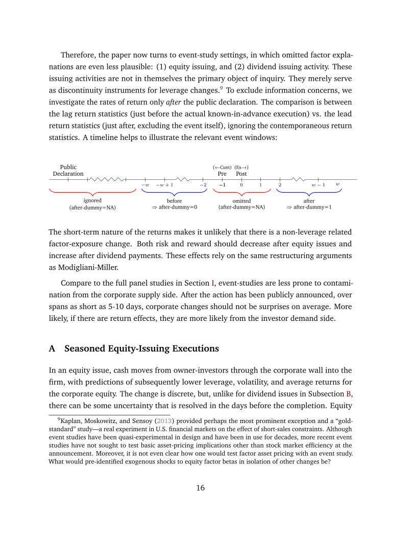
Therefore, the paper now turns to event-study settings, in which omitted factor expla-

nations are even less plausible: (1) equity issuing, and (2) dividend issuing activity. These

issuing activities are not in themselves the primary object of inquiry. They merely serve

as discontinuity instruments for leverage changes.9 To exclude information concerns, we

investigate the rates of return only after the public declaration. The comparison is between

the lag return statistics (just before the actual known-in-advance execution) vs. the lead

return statistics (just after, excluding the event itself), ignoring the contemporaneous return

statistics. A timeline helps to illustrate the relevant event windows:

PublicDeclaration

−w −w + 1 −2 −1 1 2 w − 1 w−1

(←Cum)Pre

0

(Ex→)Post

before⇒ after-dummy=0

after⇒ after-dummy=1

omitted(after-dummy=NA)

ignored(after-dummy=NA)

The short-term nature of the returns makes it unlikely that there is a non-leverage related

factor-exposure change. Both risk and reward should decrease after equity issues and

increase after dividend payments. These effects rely on the same restructuring arguments

as Modigliani-Miller.

Compare to the full panel studies in Section I, event-studies are less prone to contami-

nation from the corporate supply side. After the action has been publicly announced, over

spans as short as 5-10 days, corporate changes should not be surprises on average. More

likely, if there are return effects, they are more likely from the investor demand side.

A Seasoned Equity-Issuing Executions

In an equity issue, cash moves from owner-investors through the corporate wall into the

firm, with predictions of subsequently lower leverage, volatility, and average returns for

the corporate equity. The change is discrete, but, unlike for dividend issues in Subsection B,

there can be some uncertainty that is resolved in the days before the completion. Equity

9Kaplan, Moskowitz, and Sensoy (2013) provided perhaps the most prominent exception and a “gold-standard” study—a real experiment in U.S. financial markets on the effect of short-sales constraints. Althoughevent studies have been quasi-experimental in design and have been in use for decades, more recent eventstudies have not sought to test basic asset-pricing implications other than stock market efficiency at theannouncement. Moreover, it is not even clear how one would test factor asset pricing with an event study.What would pre-identified exogenous shocks to equity factor betas in isolation of other changes be?

16

issues can and have been cancelled. Their success is not just dependent on corporate

actions, but also on investor participation. The successful equity-issue completion could

still reveal information, despite earlier public announcements. A second contaminating

aspect is that firms often issue debt together with equity and new equity has effects that

depend on the firm’s prior capital structure (Welch (2004)). Therefore, we will cover equity

issuing activity in less detail than dividend issuing activity.

All stock return data in this eventstudy is from CRSP. The event dates are from the

Thomson SDC global issue database. In early 2016, it listed 1,131,497 offerings, of which

130,349 were corporate equity offerings. Removing IPOs yielded 97,440 offerings, of which

20,010 occurred in the United States, 17,862 were not privately placed, and 16,995 were

identified as the issue containing the entire filing amount. The need for a stock ticker,

CUSIP, a filing date, an issue date, complete filing amount, specific issue filing amount,

primary shares sold, at least 10 days between filing and offering date, and a merge with

CRSP by CUSIP, left 9,569 corporate equity offerings.10 The WRDS event-study program

yielded 7,859 offerings that had complete or near-complete stock return histories from

seven days before the offering to seven days after the offering, with about 7,600–7,800

stock return days per event day. Note again that all equity issues used in this study were

already publicly announced on the first day on which we look at stock returns.

[Insert Table 10 here: Explaining Market-Adjusted Stock Returns Around Actual Equity-Issue

Execution Dates, Given Previous Declaration]

Table 10 shows that every daily equity volatility before the issue execution is higher

than every daily equity volatility after. The average absolute rate of return from event

day –6 to –3 is 4.63%, while the average absolute rate of return from event day +3 to +6

is 3.46%. This is as it should be. Yet again, the average rate of return is not lower but

higher. In the days before the issue, the average rate of return is –0.041%/day. In the

days after, it is 0.078%/day. Together, these relations are in line with the full panel results

from Section I. Again, the risk decreases, which is expected; but the reward increases,

which is paradoxical. The panel regressions confirm the descriptive evidence and show

that the result is statistically significant. Investors receive higher average rates of return for

the less volatile equity after firms have issued equity. The chosen window from –6 to –3

versus +3 to +6 is conservative, in that pulling it one day closer to the issue date would

10Some hand-checking revealed that the CRSP data are not a good data source for the number of sharesoutstanding. CRSP is more (but not greatly) reliable at picking up reasonable number-of-shares estimates atmonth-ends than mid-months. This is also why we did not attempt to measure the dilution.

17

further increase the difference. However, this is a very short interval. Over longer intervals,

presumably as firms use the funds to execute investment plans and ordinary return noise

reasserts itself, the difference in average returns declines.

Unfortunately, there are no further large issuing or repurchasing capital structure

experiments that easily lend themselves to similar tests.11 Equity repurchases are not

suitable, because they tend to be spread over long time windows. Equity shelf-offerings are

not suitable for lack of clear event dates.12 Debt issues and repurchases do not have a clear

directional predictions for corporate net leverage.

B Dividend Payments

Dividend payments are of a smaller-magnitude than equity offerings, but also very common,

important in their aggregate effects over time, and a cleaner experiment. Again, we are

considering not announcements but dates around actual dividends payments13 of dividends

after the public declaration. We compare the behavior of stock returns just before to just

after the cum-ex transition (1) while restricting (conditioning) the sample to days on which

the declaration had already been made public many days earlier, and (2) excluding the

cum-to-ex and surrounding days themselves. This is especially important because of known

dividend-tax cum-ex drops.14

The actual dividend payments are small shocks that increase net leverage. For under-

standing the intuition that any investment actions of the firm between announcement

and payment no longer have relevance, consider two extreme examples for a firm whose

business is holding the underlying stock market index (so that it has a market-beta of 1).

In one extreme case, the firm immediately sells some index shares and puts the funds into

stock, in effect defeasing the dividend at the moment of the announcement. It is now a

bundle of stocks and bonds up to the cum date and stocks only after the ex date. Clearly,

the risk and reward should go up at the cum-ex transition. In the other extreme case, the

11One other unexploited event may be relatively rare call-forced conversions. Again, the emphasis wouldbe on the execution date, not the announcement date.

12This is also why exchange offers, as in Korteweg (2004), are not suitable for this experiment. An exchangeoffer is usually not executed on one sharp day, but over multiple weeks.

13For convenience and intuitive clarity, this study often refers to the ex-day day as the payment day. Thestudy always ignores the actual payment day on which the checks are mailed out.

14Including them would only further strengthen the results. Similarly, all reported results are robust toreasonably different event windows.

18

firm remains fully invested in the stock market up to the final moment.15 It then sells index

shares to satisfy the payment promise. At the moment of the declaration, the firm becomes

a composite of one risk-free claim worth DV and one levered claim worth 100%−DV . If the

stock-market has a rate of return of rM between the announcement and the payment, then

the risk-free claim will pay DV and the residual firm will be worth 100% · (1+ rM)− DV .

The entire risk is on the residual claim, which is riskier than 100% · (1+ rM). In net terms,[see also table with numerical

example in the appendix]

the cum-dividend stock returns are always less levered than the ex-dividend stock returns.

The cash-flow split is determined at the moment of declaration, not at the moment of

payment.16

Because the approach is quasi-experimental, the model itself can be simple. In the

exogenous leverage-risk-reward paradigm framework,

Equitypre = EquityEquity-Other + (EquityRisk-free = Dividend) ,

R̃pre = (1−δ) · R̃Equity-Other + δ · RRisk-free ,

Equitypost = EquityEquity-Other ,

R̃post = R̃Equity-Other ,

where δ is the single-event dividend yield paid at the event date. Therefore, the expected

rate of return on equity should increase by the dividend-yield scaled expected rate of return

on the prepayment equity above the risk-free rate,

E(R̃post) =�

11−δ

�

· E(R̃pre) −�

δ

1−δ

�

· RRisk-free ,

which is strictly greater than E(R̃pre) if E(R̃pre) > RRisk-free. For small δ and risk-free rates,

E(R̃)post − E(R̃pre) ≈ δ · E(R̃pre). For daily stock returns, this is a tiny but strictly positive

increase. If expected rates of return are similar, then the increase is quantitatively pinned

15Realistically, it is likely that liquidation of ordinary risky projects into cash would occur more than 5-10days before the payment, and dividend payments would be paid out of cash and short-term investments.Over time, firms would then replenish cash, either through cash flow or external financing. Farre-Mensa,Michaely, and Schmalz (2014) show that about a third of the dividends were externally financed. However,these were long-term finance patterns, and not likely to occur exactly at the dividend payment date. And,again, even if such managerial choices had had any influences on the average rate of return patterns, it isdifficult to see how such an explanation could explain both averages and volatilities.

16To have a different impact on leverage would require that firms do more than just cover the dividendpayment at the day of the dividend payment. For example, if they also sell further assets cum-day for cash,then the project leverage and risk could decline. There is no reason to believe that this should happensystematically.

19

down by the model. An empirical change larger or smaller than the prediction rejects the

exogenous-leverage paradigm.17

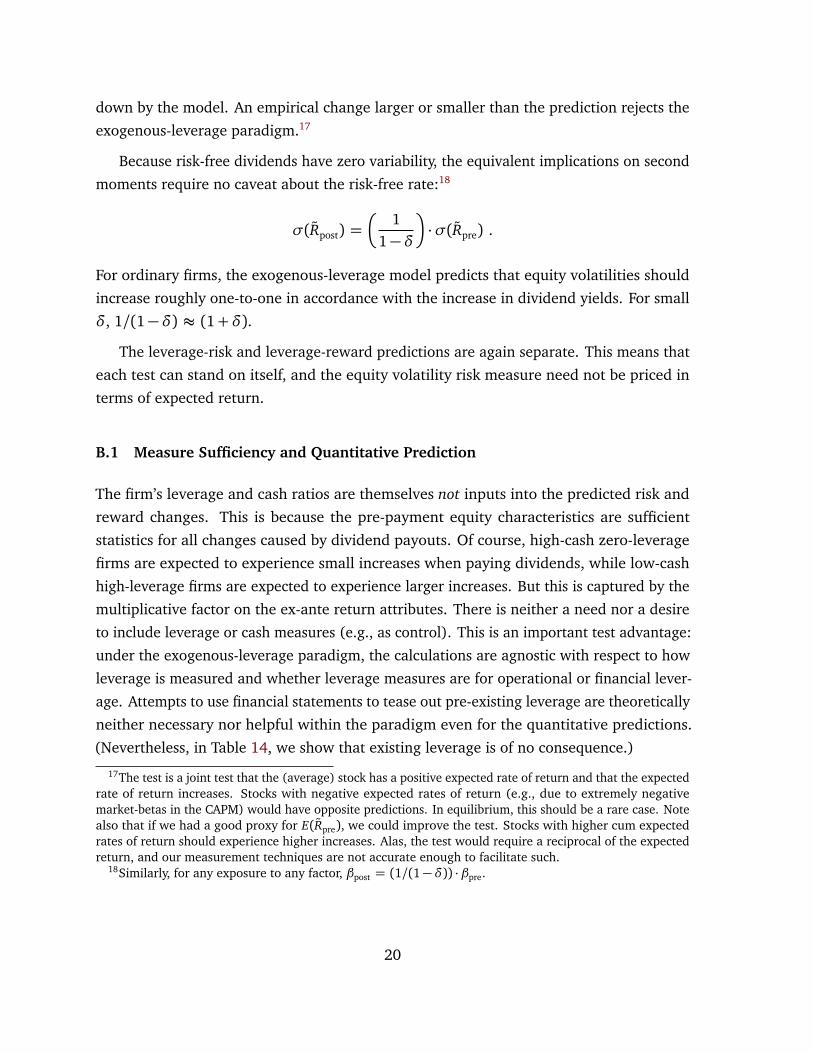
Because risk-free dividends have zero variability, the equivalent implications on second

moments require no caveat about the risk-free rate:18

σ(R̃post) =�

11−δ

�

·σ(R̃pre) .

For ordinary firms, the exogenous-leverage model predicts that equity volatilities should

increase roughly one-to-one in accordance with the increase in dividend yields. For small

δ, 1/(1−δ) ≈ (1+δ).

The leverage-risk and leverage-reward predictions are again separate. This means that

each test can stand on itself, and the equity volatility risk measure need not be priced in

terms of expected return.

B.1 Measure Sufficiency and Quantitative Prediction

The firm’s leverage and cash ratios are themselves not inputs into the predicted risk and

reward changes. This is because the pre-payment equity characteristics are sufficient

statistics for all changes caused by dividend payouts. Of course, high-cash zero-leverage

firms are expected to experience small increases when paying dividends, while low-cash

high-leverage firms are expected to experience larger increases. But this is captured by the

multiplicative factor on the ex-ante return attributes. There is neither a need nor a desire

to include leverage or cash measures (e.g., as control). This is an important test advantage:

under the exogenous-leverage paradigm, the calculations are agnostic with respect to how

leverage is measured and whether leverage measures are for operational or financial lever-

age. Attempts to use financial statements to tease out pre-existing leverage are theoretically

neither necessary nor helpful within the paradigm even for the quantitative predictions.

(Nevertheless, in Table 14, we show that existing leverage is of no consequence.)

17The test is a joint test that the (average) stock has a positive expected rate of return and that the expectedrate of return increases. Stocks with negative expected rates of return (e.g., due to extremely negativemarket-betas in the CAPM) would have opposite predictions. In equilibrium, this should be a rare case. Notealso that if we had a good proxy for E(R̃pre), we could improve the test. Stocks with higher cum expectedrates of return should experience higher increases. Alas, the test would require a reciprocal of the expectedreturn, and our measurement techniques are not accurate enough to facilitate such.

18Similarly, for any exposure to any factor, βpost = (1/(1−δ)) · βpre.

20

The predictions of the theory are quantitative: ceteris paribus, twice the dividend

payment should have twice the effect. Because both the volatility and the means tests are

scaled by the strictly positive dividend yield, they both have strictly positive predictions.

However, the volatility predictions are quantitatively larger. This is because the factor

multiplies the initial value, and the average daily volatility is about 1%, while the average

daily mean is two orders of magnitude lower—positive but near zero. The average return

prediction is near zero.

B.2 Data and Methods

All data are from CRSP, including the dividend announcement and cum-ex payment dates.

Therefore, this study is immediately and universally replicable. Except for Table 13, the

event-study uses only ordinary cash dividends, CRSP distribution code 1232. We define

the (one-event-payment) dividend yield as the dividend payment divided by the market

price of the stock at the start of the event window (either 5 or 9 days before the payment);

and winsorize it at 50%.19 The signal-to-noise ratio for detecting the effects of dividend

payments on stock returns is necessarily very small. Stock returns are very volatile on a daily

basis (1-3% per day) relative to their means (1-3 bp per day). The dividend-payment yields

are typically under 1%.20 Consequently, dividend payments predict only extremely small

changes in stock return averages and modest changes in volatility. Fortunately, there are

many observations. Unfortunately, dividends from before 1962 had to be excluded because

CRSP does not report their declaration dates. This leaves 494,643 ordinary cash-dividend

distributions from 1962 to 2015.

[Insert Table 11 here: Dividend Event-Study Descriptive Statistics]

Panel A of Table 11 shows the distribution of days between the declaration and the

cum-ex transition. CRSP reports no cases in which a firm has already declared a dividend

but fails to pay it as promised, nor are any cases familiar to me. (For further discussion of

selection biases and their possible effects, see Section III.)

The primary data restriction is the requirement of a specific number of days between

the dividend declaration and the dividend (cum-to-ex) payment date. This is because

19Winsorization affects about 300 dividend events. The results are similar if yields are winsorized at 10%,20%, or if such observations are completely removed. (This is valid, because the declaration has alreadyoccurred and therefore this criterion is based on an ex-ante known characteristic.)

20They are on the order of 1% of equity per payment in an unweighted portfolio and 1.5% of equity in thedividend-weighted portfolio. The inference is the same, regardless of weighting.

21

the maintained assumption in the experiment is that any information about the leverage

change, projects, or dividends must have already been released and thus is already known.

The event window never begins earlier than three trading days after the declaration. Events

in which the payment occurs more closely to the declaration dates are excluded. The

imposition of the requirement of availability of rate of return data from two days after the

declaration through the payment date is not a concern, because the declaration-to-ex-day

timespan is a known ex-ante (pre-event) criterion. (It does affect the kind of dividend

events from and to which the findings obtain—only distributions that would occur no

sooner than in 7 or 11 days.) Stocks that disappeared from the CRSP data set before the

dividend announcement dates are not included in CRSP. Thus they cannot affect the study,

either. However, the window choice could have raised another potential complication.

Availability of certain stocks’ returns in the window could change the composition of stocks.

In other words, some (but not other) stocks with shorter declaration notices may not mix

in the averages on different days. Permitting composition changes could cause spurious

differences in stock return moments. However, the results are robust to the treatment of

this complication in this study. It just so happened to be unimportant here. (Figure 1 and 2

will provide some support for this claim.) The paper’s main specifications are based on

stocks with 5-day and 9-day windows that have full data throughout their entire event pre-

and post-windows. The imposition of the same-firm-set requirement could have introduced

a bias if large attrition had occurred just after the payment date. This again turns out not

to be a concern. Out of 434,923 distribution events with a stock return at the payment

date, 433,375 had a stock return five days after the payment date. The reduction is just

the normal background attrition of stock returns on CRSP. Robustness checks indicate that

the results remain very robust when all stock returns on any available dates are used, which

means (for example) including stocks that were delisted during the window and even

mixing different stocks into different days.

The event study itself requires little sophistication. The event dates are not (greatly)

clustered (and we considered various [unreported] time regularity dummies), and the 1-2

week time intervals are relatively short. Moreover, the most common return adjustment

method used in this paper subtracts off the contemporaneous equal-weighted stock market

rate of return to reduce first-factor noise. The averages and standard errors can be presumed

to have been (nearly) independent draws. The results are not different if the standard errors

are calculated from the event time-series or if raw returns are used. Heteroskedasticity could

have been an issue, and thus the paper often reports both plain and White heteroskedasticity-

adjusted standard errors. Again, it matters little.

22

The study only makes sense for a few days around the dividend payment. Indeed,

when firms pay dividends every quarter, after 6 weeks, the post-payment period from the

previous payment becomes the pre-payment period for the next payment. (The pattern

already evens out after a shorter time-frame.) This design is simply not amenable to testing

long-term average return patterns.

Panel B of Table 11 shows background statistics on dividend payments and stock returns.

In the 5-day and 9-day event windows around dividend dates, stock returns have average

rates of return of 5-6 bp above the prevailing 30-day Treasury bill and 1-2 bp below

the equal-weighted stock market. In our most common specification, stock returns are

winsorized at –20% and +20%. The volatility of stock returns is about 2% per day. Dividend

yields are about 0.75% per event (i.e., about 3% per annum).

B.3 Dividend-Payment Leverage-Risk Associations

As in Section I, this section first investigates risk and then reward.

[Insert Table 12 here: Risk and Reward Changes Around Dividend Cum-Ex Transitions]

Panel A in Table 12 provides tests for a difference in the volatility of stock returns

before vs. after the dividend cum-ex transition. Each row shows the coefficients of one

panel regression. The inference is through the coefficient on an “after-payment” dummy

that takes a value of 0 before the payment and 1 after. (It can be considered NA during

the three cum-ex transition days, as well as outside the measurement interval) An earlier

draft considered many variations in the specifications of the event-window, the abnormal

return adjustment, the volatility metric, the choice of fixed effects, etc. The results were

always not just similar but nearly identical, so the table shows only some representative

variations. The coefficients on the “after-payment” dummy in A.1 through A.3 suggest

that equity volatility increases after the payment by about 1-2 bp/day, accumulating to

about 10-20 basis points over the 5-10 day event windows. The large sample ensures that

statistical accuracy is never an issue. With an average dividend payment yield of about

0.9% (see Table 11) on a base daily volatility of about 1.5%/day, the 1-2 bp/day magnitude

of the volatility increase is almost perfectly in line with the prediction of the exogenous

leverage-risk paradigm.

Lines A.4 and A.5 show coefficients of similar panel regressions that also include the

dividend yield itself plus a cross-variable on the dividend-yield before versus after the

23

event. Stocks paying higher dividends should experience greater increases. The leverage-

theory prediction fits the exogenous leverage paradigm nearly perfectly. The cross-variable

subsumes almost the entire intercept—only the higher-dividend payment events show

marked increases in volatility, and the intercept becomes insignificant. The volatility

evidence is exactly in line with (the quantitative predictions of) the leverage-risk theory

and consistent with the evidence in Section I.

B.4 Dividend-Payment Leverage-Reward Associations

Panel B provides analogous tests for the difference in average rates of returns before vs. after

the dividend cum-ex transition. The “after-payment dummy” coefficients in B.1 through

B.3 show that the average return decreases by about 3-6 bp per day. Over a window of 10

days, the estimate implies a cumulative rate of return of 30 bp less after that the payment

date. This 30 bp is high enough to be economically meaningful, but not high enough

to attract more (risky) arbitrage to eliminate it. Hartzmark and Solomon (2012) find a

similar average-return decline around dividend cum-ex transitions in their Section 4.3,

although their investigation originated from a set of related but different monthly dividend

anomalies. The positive average-rate-of-return effect is the opposite of that predicted by

the leverage-reward paradigm, but in line with the full CRSP panel evidence in Section I

and the equity issuing activity in Subsection A.

Lines B.4 and B.5 show results of similar panel regressions as A.4 and A.5 that also

include the dividend yield itself plus a cross-variable on the dividend-yield before versus

after the event. The leverage-risk-reward paradigm again predicts the opposite of what the

empirical evidence shows; and the cross-variable again largely subsumes the after-dividend

dummy: Only the higher-dividend yield stock events show the marked decrease in average

returns.21

B.5 Extended and Graphical Perspective

21Not reported, there was moderate year observation clustering, but the reported results are not drivenby the year of payment. They were similarly not driven by day-of-week effects or day-of-month effects.Including individual time-regularity dummies to control for such effects did not change the reported meansand standard deviations to the level of accuracies reported in the paper.

24

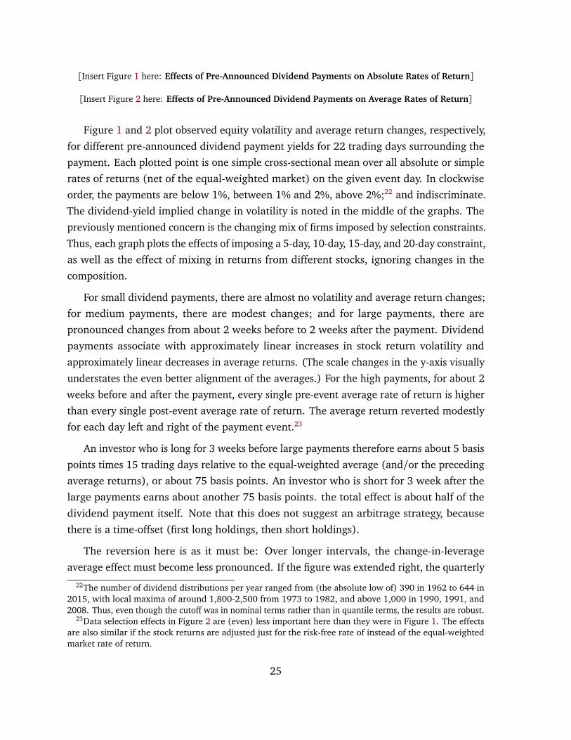
[Insert Figure 1 here: Effects of Pre-Announced Dividend Payments on Absolute Rates of Return]

[Insert Figure 2 here: Effects of Pre-Announced Dividend Payments on Average Rates of Return]

Figure 1 and 2 plot observed equity volatility and average return changes, respectively,

for different pre-announced dividend payment yields for 22 trading days surrounding the

payment. Each plotted point is one simple cross-sectional mean over all absolute or simple

rates of returns (net of the equal-weighted market) on the given event day. In clockwise

order, the payments are below 1%, between 1% and 2%, above 2%;22 and indiscriminate.

The dividend-yield implied change in volatility is noted in the middle of the graphs. The

previously mentioned concern is the changing mix of firms imposed by selection constraints.

Thus, each graph plots the effects of imposing a 5-day, 10-day, 15-day, and 20-day constraint,

as well as the effect of mixing in returns from different stocks, ignoring changes in the

composition.

For small dividend payments, there are almost no volatility and average return changes;

for medium payments, there are modest changes; and for large payments, there are

pronounced changes from about 2 weeks before to 2 weeks after the payment. Dividend

payments associate with approximately linear increases in stock return volatility and

approximately linear decreases in average returns. (The scale changes in the y-axis visually

understates the even better alignment of the averages.) For the high payments, for about 2

weeks before and after the payment, every single pre-event average rate of return is higher

than every single post-event average rate of return. The average return reverted modestly

for each day left and right of the payment event.23

An investor who is long for 3 weeks before large payments therefore earns about 5 basis

points times 15 trading days relative to the equal-weighted average (and/or the preceding

average returns), or about 75 basis points. An investor who is short for 3 week after the

large payments earns about another 75 basis points. the total effect is about half of the

dividend payment itself. Note that this does not suggest an arbitrage strategy, because

there is a time-offset (first long holdings, then short holdings).

The reversion here is as it must be: Over longer intervals, the change-in-leverage

average effect must become less pronounced. If the figure was extended right, the quarterly

22The number of dividend distributions per year ranged from (the absolute low of) 390 in 1962 to 644 in2015, with local maxima of around 1,800-2,500 from 1973 to 1982, and above 1,000 in 1990, 1991, and2008. Thus, even though the cutoff was in nominal terms rather than in quantile terms, the results are robust.

23Data selection effects in Figure 2 are (even) less important here than they were in Figure 1. The effectsare also similar if the stock returns are adjusted just for the risk-free rate of instead of the equal-weightedmarket rate of return.

25

dividend payment returns would reappear on the left.24 Firms also earn more and replenish

their cash, which should induce lower risk and reward.

Although the tests stand independently, we can also decompose the observed volatility

change (each calculated as a 4-day absolute deviation from its own mean) into one part

attributable to the dividend yield (Predicted Dividend-Related Volatility Change, PDRV∆)

and one part not attributable (Residual Dividend-Unrelated Volatility Change, URDUV∆). If

the financial mean effect is related to the same dividend-yield effect as the volatility increase,

then the PDRV coefficient should be negative. (The URDUV coefficient measures potentially

contaminating aspects.) The change in the average return from the four cum-days to the

four ex-days (Mean Return Change, MR∆) is then

MR∆ = −0.0 − 4.62× PDRV∆ + 0.23×URDUV∆

with standardized coefficients of –0.006 and +0.19, both highly statistically significant.25

Most volatility and mean returns are just dividend-unrelated correlations across stocks.

However, the increases in volatility that are attributable to the dividend-yield are different

from the more generic noise-mean associations. The effect is small, but it again suggests

that it is the exogenous volatility increase (that is due to the exogenous dividend-induced

net leverage change) that associates negatively with the average rate of return. Stocks

with more dividend-induced volatility increases showed greater declines in average returns.

This is robust to specification changes.

In sum, the increase in volatility in response to dividend payments, exactly quantitatively

in line with the prediction of the leverage-risk link, is prima-facie evidence that the financial

markets are aware of and respond appropriately to the increases in leverage caused by

dividend payments. (No alternative hypothesis seems to offer this prediction naturally.)

The leverage-risk relation is positive, but the leverage-reward relation is negative. Instead

of tiny increases in average returns, the known-in-advance payments of dividends associate

with strong decreases in average returns. The stock price increases “too much” before and

through the dividend payment, thus reducing post-payment average rates of returns relative

to prepayment average rates of return.

24Moreover, over time, cash from operations should flow back into the firm and reduce leverage. Notealso that the effect documented in the paper is a reduction in average returns, unlike the effects documentedin studies of post-announcement or dividend payments, which generally show increases in average returns.This is not inconsistent. The study designs are simply quite different.

25Stock return means are difficult to explain, and in this cross-sectional specification, each event is only oneobservation. A two-step panel regression approach yields higher T-statistics, but is more difficult to interpret.

26

Dividend payments are the most cleanly identified test of mean and volatility changes

around leverage changes. Therefore, we now look at some remaining pragmatic concerns

that deserve further empirical investigation, related to dividend taxes, the types of dividend

paid, the year-to-year changes, the surprises investors experience, the firms’ leverage

positions (despite the theoretical irrelevance), and liquidity and trading considerations.

B.6 Concerns About Dividend Taxes

The dividend experiment is not about corporate capital structure or dividend payout policy.

Answering different questions, this paper does not share event periods with earlier corporate

finance work. That is, unlike earlier dividend literature (explored and reviewed in, e.g.,

Michaely, Thaler, and Womack (1995) or Allen and Michaely (2003)), my paper explores

the stock returns around neither the dividend announcement dates nor the dividend cum-ex

dates.

There is theory and evidence that show that personal dividend taxes play an important

role on the (single) cum-ex day rate of return (e.g., Michaely (1991), Poterba (2004),

Chetty and Saez (2005), Chetty, Rosenberg, and Saez (2007)). There is no coherent theory

for a “slow tax effect.” Investor clientele trading effects could blunt even the cum-ex tax

effect, but the empirical evidence suggests that clientele trading, even if present, is not

of first-order importance to the stock return process. There seems to be a full response

on the single cum-to-ex day, indicating an effect in line with prevailing dividend tax rates.

To be a coherent explanation, somehow, many low-tax investors would have to buy into

dividend-paying stocks sooner than necessary, selling investors would have to be scarcer

than buying investors, there would still have to be enough buyers to have a price impact,

and the prices themselves would have to fail to adjust instantly (i.e., before the event

window) despite full advance common knowledge in the market. Moreover, somehow,

there would have to be an impact on volatility opposite to the impact on average returns.

Nevertheless, we can examine whether there is an empirical link between the surrounding

stock returns documented in my paper and dividend taxes.

[Insert Figure 3 here: Year-by-Year Coefficients Explaining Stock Return Moments after Payment and

highest Individual Dividend Income Tax Rates]

Because non-anonymous stock holding and trading data is not available, my tests cannot

investigate tax-exempt holdings directly. I can investigate whether the effects were stronger

when dividend taxes were more important. Figure 3 shows that the highest Federal income

27

dividend tax rates were fairly steady from 1962 to 1982 (around 65-70%), declined all

the way down to 15% from 1982 to 2013, and finally increased again to 20% and then

24%. In 1986 and 2003, there were particularly sharp declines in tax rates. The two lower

panels plot the most interesting OLS coefficients (on the bivariate-only post-ex dummy and

on the multivariate cross-variables) when run year by year. The plots show that although

a tax-related phenomenon may have contributed a little to the coefficients, the relation

between the dividend-tax rates and the before-after dummy is weak. The dummy and

the cross-coefficients show no clear or pronounced trends corresponding to large changes

in prevailing dividend tax rates.26 There is no time association between years in which

dividend taxes are high or low and the 5-day effects documented in the paper. Volatility

always increases with dividend payments, average returns always decrease.

[Insert Table 13 here: Different Types of Dividends]

Not all dividends are taxable. About 1 in 50 dividend payments are treated as a return

of capital and not taxed. In these cases, tax imperfections can be excluded as potential

explanations. Table 13 shows that non-taxable dividend distribution suffer almost identical

declines in average rates of return as taxable dividend distributions.

[Insert Table 14 here: Cum-To-Ex Association?]

Finally, it is an interesting question whether the effect documented in my paper is related

to the cum-ex drop. This could be the case, e.g., if the cum-to-ex return drop itself is a

noisy proxy for tax or perhaps other unspecified effects, and the same effects influences the

expected returns and volatilites around the event. In the sample, the cum-to-ex average rate

of return was about 25bp—implying an average effective tax rate of about 25/90 ≈ 28%—

with a standard deviation of 212bp. The regressions Table 14 control for the cum-to-ex

drop. Firms with higher cum-to-ex rates of return also have lower post-event mean returns.

However, controlling for the cum-ex stock return has no effect on the inference about the

difference between pre-cum and post-ex rates of return (the dummy). The cum-to-ex return

drop phenomenon is unrelated to the further changes in average rates of return around

dividends that are documented in my paper.

All evidence suggests that tax effects do not play an important role in the two weeks

left and right of but excluding the cum-ex date.26Unreported regressions explaining the volatility of year-by-year “after the event dummy” coefficients

(and cross-coefficients) with dividend taxes have adjusted R2s that are negative. Regressions explaining theaverage return year-by-year “after the event dummy” coefficients (and cross-coefficients) with dividend taxeshave adjusted R2’s of 3-5%.

28

B.7 Other Plausible Concerns

Pre-Existing Leverage: Though similarly atheoretical, we can investigate whether more

levered firms experience more of an effect. Panel B in Table 13 divided stocks into three

groups based on their Compustat total liabilities (LT) net of cash, divided by total assets

(AT), at the end of the previous fiscal year. The empirical evidence is not clear. Higher-

liability firms seem seem to have a lesser mean drop than low- and medium-liability firms,

but the cross-coefficient is about the same. Pre-existing leverage does not seem to be a

promising direction for further investigation.

Surprises, Endogeneity, Selection, Survivorship: The design of this experiment is

resistant to project endogeneity concerns. By the day that stock returns are beginning

to be included in the stock return calculations, the impending dividend-leverage change

has already been determined and announced. Publicly-traded company are not known to

retract dividends after they have been declared. It is implausible that investors increase

in belief that payments would occur in the days before the payment date. Even if the

dividend payment were not paid but instead completely dissipated, in order to explain the

documented lower average returns, non-payments would have to occur about 1-in-100

times, with hundreds of companies failing to pay declared dividends every year.27

Nevertheless, we can push the endogeneity consideration even further backwards. We

can separate the sample into dividends payments that are regular and long-standing (i.e.,

where investors could commonly assess that a dividend would be paid months in advance)

versus payments that are new and special. The evidence in Table 13 shows there is no

difference. (The coefficient for special dividends is about four times higher because the

yield typically paid out in special dividends is about four times higher.) Regularity of

payments does not seem to be a promising direction for further investigation.

[Insert Figure 4 here: Explaining Average Trading Liquidity Patterns around Previously Declared

Payment Dates]

Liquidity and Trading: Although prices can change in the absence of trading, to the

extent that investors in the aggregate had time-varying preferences, they could leave an

imprint on trading activity. For example, some investors could trade into dividend-paying

27The leverage-reward finding could be consistent with firms moving large amounts of risky stock-marketholdings into cash the day after the payment, thus becoming safer. However, beside the fact that such behavioris not known, it is also inconsistent with the leverage-risk findings.

29

stocks before the payment and then trade out again. This could but need not be rational

(e.g., tax trading). Table 4 plots the day-by-day average log number of trades and log

dollar volume (also obtained from CRSP). There is the tiniest of up-blips in liquidity on

days –1 and 0, but there are no increasing or decreasing trends either before or after the

payment. In the event windows used for calculating volatilities and average returns, there

is no increasing buying pressure before the payment or decreasing selling pressure after

the payment. Not shown, in unreported regressions, the after-payment dummy regression

coefficients in panel regressions explaining either liquidity variable is insignificant. It is

a fair characterization that prices seemed to move without unusual extra trading volume

patterns. Although the sophistication of the trading tests could be enhanced, liquidity and

trading does not seem to be a promising direction for further investigation.

B.8 Less Plausible Concerns

Timing and Managerial Response: Even if corporate managers had the forecasting ability

to time their dividend payments to occur on days when average stock returns would then be

lower (which is implausible), naive versions of this hypothesis would require that investors

would not recognize this already at the moment of announcement. Dividend catering, as

in Baker and Wurgler (2004), should similarly be reflected on the announcement date and

not occur around the payment date, either. Managerial response misspecification concerns

seem implausible.

Underlying Investment Activities: Although it is the defeasance of the dividend that

should matter and not the actual underlying risky investment patterns, correlated changes

in risk patterns—other than those directly due to the leverage change—seem unlikely. And

again, even an explanation based on the firm aggressively buying stock futures before the

dividend payment and liquidating them afterwards cannot explain both mean decreases

and volatility increases.28 Growth options, as in Gomes and Schmid (2010), are unlikely to

explain simultaneous increases in variance and decreases in means. While plausible and

consistent in their context, it seems implausible in this context.

Intrinsic Leverage or Volatility Preferences: Investors may like the increases in id-

iosyncratic volatility so much that they bid up the price, leaving lower average rates of

return after the payment-induced risk-increase. In unreported regressions, if the rate of re-

turn is explained with the absolute rate of return and the cross-effect post-payment dummy,

28Besides, if firms could follow strategies with higher average returns and lower risk, why would they stopdoing so after the dividend payment?

30

it appears that it is the stocks with the higher post-event volatilities that experienced lower

average returns after the payments.29 This suggests again that investors earned lower

average rates of return when volatility increased because of the payment, and perhaps

specifically because the payment increased volatility (Goyal and Santa-Clara (2003)). Al-

though such a theory would also suggest that managers could increase shareholder value by

gambling more aggressively, the problem remains that the option-induced higher expected

rates of return should have been reflected at the dividend declaration itself. This seems

implausible.

III Speculative Discussion

This paper has already repeatedly mentioned the primary perfect-market explanation—a

mysterious risk-factor that not only declines in leverage, but declines systematically and

so much after the leverage increase that it can reverse the direct positive average rate of

return implication. The risk-factor exposure decline in leverage would somehow further

increase simultaneously with firm volatility, although the latter happens to be quantitatively

exactly in line with the leverage-change prediction. The observed risk change constellation

would also be puzzling from the perspective of most corporate finance theories, in which

managers typically want to reduce not their systematic factor exposures but their own

volatilities (in order to reduce financial distress costs). And on a pragmatic basis, even

if managers (unlike academics) understand this mysterious risk factor, it is unclear howmanagers would mechanically adjust their leverage to reflect both the decreasing factor

risk and increasing own risk effects simultaneously.

The leverage anomaly here seems related to the idiosyncratic volatility anomaly in Ang

et al. (2006). Higher risk seems to be associated with lower average returns. However,

the basic primitive in my paper is different, and there is some evidence that the effects are

different. Leverage is important even when risk is controlled for.

The alternatives to the perfect-market explanation are imperfect-market explanations, in

which investors bid up the prices of stocks increasing leverage and thereby drive down sub-

sequent average rates of return. These changes would be as puzzling as “non-arbitrageble.”

There are two potential market imperfection that come to mind.

29When the mean is not-zero, then there is an association between returns and absolute returns. It should,however, be weak.

31

Investor Preferences: The first reason is behavioral. Investors become infatuated with

low leverage. When there are dividend payments, they bid up the price a little too

much before the dividend. Investors behaved as if they had wanted to be present just

in time to receive the dividends. The historical average rates of return were thus not

reflective of investors’ true expected rates of return, because investors were naive

and non-anticipatory. Put differently, the return patterns could have been caused by

a financial market which was non-blissfully ignorant of risks and outlooks, with more

levered companies having been exposed to more post-payment risk (and malaise)

more frequently. Thus, higher-leverage dividend-paying stocks could have had lower

post-payment average rates of return, with financial market prices not taking this

added risk appropriately into account.

Investor Agency: The second reason is agency-related. This is particularly prominent in

Harris, Hartzmark, and Solomon (2016), which finds that mutual funds may have

had preferences for dividends, because dividends to mutual-fund investors labeled

as such are required to come from dividends in the underlying stock holdings.30

Mutual funds report twice as much in quarterly dividends as their quarterly reported

holdings would justify. Harris-Hartzmark-Solomon show that this “juicing” harms

fund investors. (Incidentally, it is the opposite of rational tax trading, where it is the

tax-exempt that should gravitate towards dividend payments.) They also note that

this agency hypothesis pushes mutual funds into the dividend-preference direction

because their retail investors seem, in turn, to be irrationally attached to receiving

payments labeled dividends. The two hypotheses blend.31

These preferences explanation are ad-hoc, but they are not entirely implausible—Lamont

and Thaler (2003) document even stranger law-of-one-price violations probably also due

to investor-demand effects. Their evidence appears in a small number of isolated stocks

with close-to-indisputable value evidence (and, of course, absence of easy arbitrage). It is

sometimes discounted as mere “aberrations” when investors were particularly irrational.

In contrast, the effects documented in my paper are more pervasive. Although Baker,

30Mutual funds can still pay out funds, but they would not carry the dividend label. Quoting Harris-Hartzmark-Solomon, “while distributing cash to the fund’s shareholders is easy, such distributions only canbe labeled as ‘dividends’ if they correspond to dividends received by the fund on its underlying securities.This constraint arises because funds must satisfy a ‘pass-through rule’ that requires that they distribute allgains and losses each year to avoid paying corporate income taxes.”

31Hartzmark and Solomon (2012) compares expected dividend with non-dividend payers and focuses onan extended dividend anomaly that is also unlikely to be explained by risk. However, as already mentioned,in Section 4.1, it does show evidence related to the mean effect around dividend payments.

32

Hoeyer, and Wurgler (2016) explore Gomes-Schmid-like long-run performance and have

overlapping implications (e.g., riskier firms choosing lower leverage), Baker-Hoeyer-Wurgler

interpret the evidence as suggestive of risk-leverage mispricing. They then consider both

the perspective and optimal behavior of the corporation.32

A Other and Simultaneous Explanations

The imperfect-market behavioral investor preference evidence here and elsewhere should

not be viewed as mutually exclusive with the perfect-market hypotheses in Fama and French

(1992) or Gomes and Schmid (2010). More than likely, the economic forces all play roles

in the association of leverage with risk and reward, possibly differently at different times

or for different firms. Economic theories often hold in some contexts, but not others. Like

all economic tests, the empirical findings are context specific, and the measured effects are

only “net.”

There is however one shortcoming in the earlier “asset supply side” arguments in Fama

and French (1992) and Gomes and Schmid (2010) worth mentioning. They embraced

the perfect-market rational paradigm with too little skepticism. They failed to allow for

and/or to embed less appealing “investor demand side” alternatives that can play roles,

too. What if financial markets are imperfect and it is not risk but other characteristics

that investors prize? What if financial markets simply did not respond (appropriately) to

financial leverage? What if investors or their investment agents “liked” some (aspects of)

firms too much?

The evidence in my paper suggests that more skepticism is appropriate when interpreting

previous long-run empirical evidence. Before concluding that the associations between

leverage and returns are solely or primarily due to information revelation or corporate

responses to growth options based on book-to-market moments, it seems appropriate not

to make asset supply effects the entire working hypothesis. One should not ignore investor

demand effects, including non-arbitrageable, collectivist, imperfect-market (tax, agency)

and/or behavioral investor preferences.

32The findings are also not inconsistent with the views expressed in Hoberg and Prabhala (2009) that thevolatility increases in Campbell et al. (2001) could have had direct corporate finance implications—thoughperhaps in the opposite direction.

33

Future tests of the Gomes and Schmid (2010) option-growth theory could also benefit

(1) from tests that measure growth options and leverage responses more directly33 and (2)

break out other possible investor demand-based forces. Supply and demand effects can lead

to interestingly similar and different conclusions. Similar critiques can be offered for other

reflexive perfect-market interpretations. Could the Fama and French (1992) value factor

be similar to low leverage, offering high average rates of return without commensurate

declines in risk? Unfortunately, in the absence of discrete shocks to value (as there are to

leverage), this is difficult to determine.

B Odds and Ends

• The methods and results proposed in my paper are relevant not only in the (not so

narrow) leverage test context. Consider any other deep risk factor (e.g., a consump-

tion hedge or HML) that is supposed to explain reward. It should be amplified by

leverage. Thus, variation in leverage can be used as an instrument to improve tests. If

either the mean or factor loading is not appropriately disturbed by leverage changes,

it is implausible that this factor should be viewed as a valid priced equilibrium risk

factor. Future research could thus not only test factor responses, but design factor

tests that identify off of leverage changes or instrument factor tests.

• The leverage-risk-reward relation is not just important in the asset-pricing realm.

Leverage is also a fundamental building block in corporate finance. If increases in

leverage do not induce increases in required reward, it would change capital-structure

tradeoffs, too. Ceteris paribus, firms should then issue even more debt, as equity

would no longer suffer commensurate risk externalities.

• My paper relates loosely to a strand of literature about the CAPM and the security-

market line. However, these papers are primarily concerned about the underper-

formance of high-beta vs. low-beta stocks, observed as early as Black, Jensen, and

Scholes (1972). Based on the Black (1972), Black (1993, p.76) proposes leverage

aversion of borrowing-constrained investors as one possible explanation for the better

performance of low-beta stocks.34 Asness, Frazzini, and Pedersen (2012) improve

33Growth options in this context are typically not inferred from supply-side aspects in the firm, but fromindirect inference measures such as book-to-market ratios. Although this is plausible, demand forces couldalso impact market prices and thus effect book-to-market ratios.

34Black also briefly discusses the reaction of stocks to leverage offerings on the announcement date itself asevidence for a preference of investors in favor of debt financing. However, this is usually attributed primarilyto news about the firm.

34

on Black’s early work and also call the underperformance of stocks relative to bonds

“leverage aversion.” However, at their broad asset-class level, the Sharpe-ratio differ-

ential of 0.47 vs 0.35 seems more in line with the tax differential between capital

gains and interest payments than with leverage aversion. Frazzini and Pedersen

(2014) present more convincing evidence that higher beta stocks have pervasively

lower alphas in many different markets and also within equally-taxed asset classes.

Importantly, these papers mostly mean investor leverage when they discuss leverage

aversion and leverage constraints, and not corporate leverage. Consequently, unlike

my own paper, they are not looking at the same evidence about the stocks’ corporate

leverage, much less do they investigate average return and idiosyncratic risk patterns

associated with changes in corporate leverage. However, both their and my findings

could be related to an intrinsic like or dislike of risk and leverage.35

IV Conclusion

Consumption asset-pricing tests are theoretically well identified, but their empirical failures

to explain the cross-section of stock returns can be blamed on ignorance of the relevant risk

metrics. This makes them difficult to reject. Empirical factor models (such as Fama and

French (2015)) can explain large average stock return differentials, but their theoretical

bases remain controversial. In both cases, misidentification of risk factors is a first-order

concern. If risk proxies (say, beta, momentum, or value) fail to explain average returns, then

it “only” raises skepticism about whether the proxies were good, and not about whether

the perfect-market theory is wrong. The risk proxies are themselves largely endogenous

and continuous. There are no academic papers that have investigated quasi-exogenous

discrete shocks to these proxies.

Leverage as a risk proxy has important advantages over deeper risk factors and thus

risk-reward tests. It is solidly identified. Its is more resistant to measurement concerns

and problems stemming from academic ignorance. It works regardless of the deeper factor

structure. It offers empirical identification strategies that stem from active and discrete

managerial interventions. Some of these tests offer discrete changes. And empiricists

can choose among tests with different degrees of coverage, endogeneity, information

contamination, and corporate response concerns.

35Another loose relation is to a new literature that uses information to time strategies (e.g., Daniel andMoskowitz (2016)). A prominent timer is the aggregate time-series volatility, as in Moreira and Muir (2016).

35

The leverage-risk-reward paradigm predictions are also not deep. They require no hyper-

sophistication and knowledge by investors (itself exceeding that of the most sophisticated

financial economists). They are simply that investors should suffer more risk when firms

lever up and thus earn higher average returns. Yet the evidence in my paper rejects this. It

is not a matter of ignorance or test power: The effect of leverage always appears clearly in

firm’s own equity volatility. But average stock returns paradoxically decrease in leverage. A

simple restatement of the puzzle is that investors recognize the increase in risk but like the

higher leverage so much that they bid up stock prices too much—the opposite of leverage

aversion. The question for which no one has an answer is: Why?

This throws down the gauntlet for a theory capable of tying together the basic building

blocks of asset pricing—corporate leverage, risk, and reward. The theory needs to explain

the following:

• Average return decreases in leverage levels, after (many) controls.

• Equity volatility increases in corporate leverage.

• Average return decreases in leverage changes.

• Average return is also lower when leverage increases together with equity volatility

(and market-beta).

• The effects appear even when leverage changes cannot be due to managerial actions

but can only be due to stock price changes (most of which are primarily value shocks

and not primarily reflections of expected returns).

• The effects appear even when leverage changes are sharp and discrete, on time-

horizons as short as a few days (where underlying corporate changes [from the

supply side] should be be less important than investor preferences [from the demand

side]).

• And they appear even when it cannot possibly be due to contaminating new informa-

tion.

After this theory has identified this mysterious factor that can explain these effects—i.e.,

a factor that would (co-)decrease so strongly with leverage that it could explain lower

average returns as leverage increases—we would of course still want to know why this

factor would decrease in leverage to begin with.

36

References

Acharya, Viral V., Heitor Almeida, and Murillo Campello (2007). “Is cash negative debt? A

hedging perspective on corporate financial policies”. In: Journal of Financial Intermedia-tion (16), pp. 515–554.

Allen, Franklin and Roni Michaely (2003). “Payout Policy”. In: North Holland, pp. 337–430.

Ang, Andrew et al. (2006). The Cross-Section of Volatility and Expected Returns.Asness, Clifford S., Andrea Frazzini, and Lasse Heje Pedersen (2012). “Leverage Aversion

and Risk Parity”. In: Financial Analysts Journal 68.1, pp. 47–59.

Baker, Malcolm, Mathias F. Hoeyer, and Jeffrey Wurgler (2016). The Risk Anomaly Tradeoffof Leverage. Tech. rep. NBER and Harvard Business School.

Baker, Malcolm and Jeffrey Wurgler (2004). “A Catering Theory of Dividends”. In: 59 (3),

pp. 1125–1165.

Bartov, Eli, Mark L. DeFond, and Yaniv Konchitchki (2013). The Consequences of UntimelyQuarterly and Annual Financial Reporting. Tech. rep. NYU, USC, and UCB. URL: https://ssrn.com/abstract=2368413.

Becker, Bo, Marcus Jacob, and Martin Jacob (2013). “Payout taxes and the allocation of

investment”. In: Journal of Financial Economics 107.1, pp. 1–24.

Bhandari, Laxmi (1988). “Debt/equity ratio and expected stock returns: Empirical evidence”.

In: The Journal of Finance 43, pp. 507–528.

Black, Fischer (1972). “Capital Market Equilibrium with Restricted Borrowing”. In: Journalof Business 45.3, pp. 444–455.

— (1993). “Beta and Return”. In: Journal of Portfolio Management 20.1, pp. 8–18.

Black, Fischer, Michael C. Jensen, and Myron S. Scholes (1972). “The Capital Asset Pricing

Model: Some Empirical Tests”. In: Studies in the Theory of Capital Markets. Ed. by

Michael C. Jensen. Praeger.

Campbell, John Y. et al. (2001). “Have Individual Stocks Become More Volatile? An Empirical

Exploration of Idiosyncratic Risk”. In: 56.1, pp. 1–43.

Chetty, Raj, Joseph Rosenberg, and Emmanuel Saez (2007). “The Effects of Taxes on Market

Responses to Dividend Announcements and Payments: What Can We Learn from the

2003 Dividend Tax”. In: Cambridge University Press, pp. 1–33.

Chetty, Raj and Emmanuel Saez (2005). “Dividend Taxes and Corporate Behavior: Evidence

from the 2003 Dividend Tax Cut”. In: The Quarterly Journal of Economics 120.3, pp. 791–

833. DOI: 10.1093/qje/120.3.

Daniel, Kent and Tobias J. Moskowitz (2016). “Momentum Crashes”. In: Journal of FinancialEconomics 122.2, pp. 221–247.

37

Fama, Eugene F. and Kenneth R. French (1992). “The Cross-Section of Expected Stock

Returns”. In: The Journal of Finance 47 (2), pp. 427–465.

— (1998). “Taxes, financing decisions, and firm value”. In: The Journal of Finance 53,

pp. 819–843.

Fama, Eugene R. and Kenneth R. French (2015). “A five-factor asset pricing model”. In:

Journal of Financial Economics 116, pp. 1–22.

Farre-Mensa, Joan, Roni Michaely, and Martin C. Schmalz (2014). Payout Policy. Tech. rep.

Harvard Business School, Cornell University, and University of Michigan.

Frazzini, Andrea and Lasse Heje Pedersen (2014). “Betting against beta”. In: Journal ofFinancial Economics 111.1, pp. 1–25.

Gomes, Joao F. and Lukas Schmid (2010). In: The Journal of Finance 65.2, pp. 467–494.

Goyal, Amit and Pedro Santa-Clara (2003). “Idiosyncratic Risk Matters!” In: The Journal ofFinance 58 (3), pp. 975–1007.

Harris, Lawrence, Samuel M. Hartzmark, and David H. Solomon (2016). “Juicing the

Dividend Yield: Mutual Funds and the Demand for Dividends”. In: Journal of FinancialEconomics 116 (3), pp. 433–451.

Hartzmark, Samuel M. and David H. Solomon (2012). “The Dividend Month Premium”. In:

Journal of Financial Economics 109 (3), pp. 640–660.

Harvey, Campbell R., Yan Liu, and Heqing Zhu (2016). “... and the Cross-Section of Expected

Returns”. In: Review of Financial Studies 29.

Herskovic, Bernard et al. (2016). “The Common Factor in Idiosyncratic Volatility: Quanti-

tative Asset Pricing Implications”. In: Journal of Financial Economics 119.2, pp. 249–

283.

Hoberg, Gerard and Nagpurnanand R. Prabhala (2009). “Disappearing Dividends, Catering,

and Risk”. In: Review of Financial Studies 22.1, pp. 79–116.

Jacob, Martin, Roni Michaely, and Maximilian A. Mueller (2016). The Effect of ConsumptionTaxes on Corporate Investment. Tech. rep. WHU and Cornell.

Kaplan, Steven N., Tobias J. Moskowitz, and Berk A. Sensoy (2013). “The Effects of Stock

Lending on Security Prices: An Experiment”. In: The Journal of Finance 68 (3), pp. 1891–

1936.

Korteweg, Arthur (2004). Financial leverage and expected stock returns: Evidence from pureex change offers. Tech. rep. Stanford University and University of Southern California.

Lamont, Owen A. and Richard H. Thaler (2003). “Anomalies: The Law of One Price in

Financial Markets”. In: Journal of Economic Perspectives 17.4, pp. 191–202.

Michaely, Roni (1991). “Ex-Dividend Day Stock Price Behavior: The Case of the 1986 Tax

Reform Act”. In: The Journal of Finance 46.3, pp. 845–859.

38

Michaely, Roni, Richard H. Thaler, and Kent L. Womack (1995). “Price Reactions to Dividend

Initiations and Omissions: Overreaction or Drift?” In: The Journal of Finance 50.2,

pp. 573–608.

Moreira, Alan and Tyler Muir (2016). Volatility Managed Portfolios. Tech. rep. Yale and

UCLA.

Pinkowitz, Lee, Rene Stulz, and Rohan Williamson (2006). “Does the Contribution of

Corporate Cash Holdings and Dividends to Firm Value Depend on Governance? A

Cross-country Analysis”. In: The Journal of Finance 61 (6), pp. 2725–2751.

Poterba, James (2004). “Corporate Payout Policy”. In: American Economic Review 94.2,

pp. 171–175.

Sialm, Clemens (2009). “Tax Changes and Asset Pricing”. In: American Economic Review99.4, pp. 1356–83.

Welch, Ivo (2004). “Capital Structure and Stock Returns”. In: Journal of Political Economy112.1, pp. 106–31.

— (2011). “Two Common Problems in Capital Structure Research: The Financial-Debt-To-

Asset Ratio and Issuing Activity Versus Leverage Changes”. In: International Review ofFinance 11.1, pp. 1–17.

39

Table 1: Spread of Debt-Ratio Levels and Changes

tbl:panel-descriptives in v4-xsect/panel-descriptives.tex, January 31, 2017

Panel Standard Deviations Quartile MeansMean All Xsect TS Q #1 Q #4

Debt-Ratio Levels:mknegcash 0.910 0.115 0.103 0.045 0.804 0.981mklev 0.240 0.253 0.239 0.087 0.046 0.496mkliab 0.365 0.269 0.249 0.090 0.134 0.622

bknegcash 0.866 0.176 0.148 0.053 0.707 0.974bklev 0.268 0.257 0.252 0.086 0.060 0.530bkliab 0.410 0.260 0.245 0.083 0.181 0.646

Debt-Ratio Simple Changes:schg.mknegcash 0.000 0.066 0.060 0.048 –0.053 0.053schg.mklev 0.005 0.113 0.106 0.080 –0.087 0.105schg.mkliab 0.008 0.109 0.100 0.082 –0.084 0.107

schg.bknegcash 0.002 0.072 0.066 0.053 –0.057 0.065schg.bklev 0.004 0.108 0.103 0.076 –0.084 0.102schg.bkliab 0.007 0.098 0.091 0.073 –0.076 0.097

Debt-Ratio Extreme Changes:xchg.mklev 0.030 0.678 0.605 0.381 –0.401 0.527xchg.bklev 0.036 0.622 0.581 0.351 –0.349 0.508

Instrumented Debt-Ratio Changes Non-IV Q MeansR.schg.mklev –0.005 0.064 0.058 0.042 –0.054 0.046 –0.043 0.049R.schg.mkliab –0.008 0.075 0.067 0.053 –0.068 0.055 –0.038 0.054

Explanations: These are descriptive statistics for the key independent debt-ratio variables. All data are fromCompustat and CRSP, 1962–2015. There are six measures of indebtedness: “mk”-based measures use market-basedequity values (preferably from Compustat, but also CRSP if former is not available); “bk”-based measures usebook-based equity values. “negcash” is one minus cash (preferably CHE, but CH if not available) divided by bookor market-assets. “lev” is financial leverage: netdebt/(netdebt + equity), where netdebt is debt (itself [Compustat]DLTT plus DLC) minus cash, and equity is either the (modestly adjusted) book value of equity (CEQ) or a market-value of equity from Compustat or CRSP. “liab” are liabilities (LT) net of cash divided by total assets (AT). Alldebt-ratios are also winsorized to lie between 0.001 and 0.999. The first four rows describes leverage in levels, thenext four rows in simple changes, the next two rows in “extreme” changes, and the final two rows for stock-returnimputed capital-structure changes (explained later). The bottom right four values show the non-instrumentedchanges in debt ratios for the two quartiles. The quartiles themselves are based on a sort of stocks to spread thekey debt ratio (or ratio change) while maintaining balance by year and firm-size. That is, stocks are sorted byyear, assets, and then by the variable itself. Within each group of four stocks, the least levered stock is assigned toquartile #1, the highest to quartile #4.

40

Table 2: Corporate Debt-Ratio Levels and Subsequent Rates of Return

tbl:famatables-lvls in v4-xsect/famatables-lvls.tex, January 31, 2017

Panel A: Fama-French Alphas for Quartile Portfolios Spread By Debt Ratios, Year and Book-Asset Balanced

Raw XMKT XMKT,SMB,HMLXMKT,SMB,HML,

RMW,CMAXMKT,SMB,HML,RMW,CMA,UMD

Alpha (T-stat) Alpha (T-stat) Alpha (T-stat) Alpha (T-stat) Alpha (T-stat)

mknegcash –0.395 (−5.41) –0.316 (−4.70) –0.345 (−5.45) –0.448 (−7.74) –0.464 (−7.91)mklev 0.076 (+0.74) 0.128 (+1.26) –0.145 (−1.86) –0.200 (−2.56) –0.138 (−1.78)mkliab 0.154 (+1.43) 0.212 (+2.00) –0.078 (−0.98) –0.151 (−1.92) –0.107 (−1.36)

bknegcash –0.186 (−2.02) –0.077 (−0.93) –0.231 (−3.33) –0.365 (−5.82) –0.371 (−5.82)bklev –0.139 (−1.70) –0.120 (−1.46) –0.306 (−4.37) –0.336 (−4.79) –0.291 (−4.14)bkliab –0.072 (−0.78) –0.039 (−0.42) –0.242 (−3.04) –0.323 (−4.26) –0.300 (−3.91)

Panel B: Fama-Macbeth Regressions, Coefficient Reported Only For Key Debt Measure

Solo Solo Incl. Cntrls Incl. Cntrls (TSσ)DT Qrtl (T-stat) DT Ratio (T-stat) DT Ratio (T-stat) DT Ratio (T-stat)

mknegcash –0.116 (−4.61) –1.778 (−4.54) –1.411 (−3.96) –1.404 (−3.93)mklev –0.030 (−0.93) –0.235 (−1.23) –0.418 (−2.57) –0.417 (−2.58)mkliab 0.002 (+0.05) 0.122 (+0.59) –0.218 (−1.22) –0.220 (−1.23)

bknegcash –0.069 (−2.27) –0.755 (−2.41) –1.140 (−3.92) –1.139 (−3.92)bklev –0.088 (−3.31) –0.583 (−3.62) –0.455 (−3.19) –0.453 (−3.19)bkliab –0.057 (−1.92) –0.386 (−2.07) –0.369 (−2.30) –0.366 (−2.29)

Explanations: This table shows the (abnormal) post-measurement average rate of return performance, in percent,for stocks with high debt-ratios levels net of the converse. The four debt ratios (leverage and liability ratios in bothmarket and book values) are explained in Table 1. The dependent stock returns begin four to five months after thefiscal year end, and usually last for twelve months. All data is from Compustat and CRSP, 1962–2015.

Panel A shows Fama-French intercepts for zero-investment portfolios sorted into quartiles, long high-leverage, shortlow-leverage, both year- and asset-balanced.

Panel B shows Fama-Macbeth coefficients and T-statistics (Newey-West with 1 Lag) on debt ratios, using the sameleverage quartile indicators (in the first two data columns), or the debt-ratio itself (in the second two data columns),or the debt ratios themselves either when no other variables or when further variables are included (coefficientsnot reported): the book-market ratio, the firm size, investment, operating profitablity, and the rate of return inlagged months 2–12 (non-advancing) with respect to the fiscal year (in the third two data columns).

Interpretation: Stocks with higher book-leverage have worse subsequent performance. Stocks with higher market-leverage have worse performance only with further controls.

41

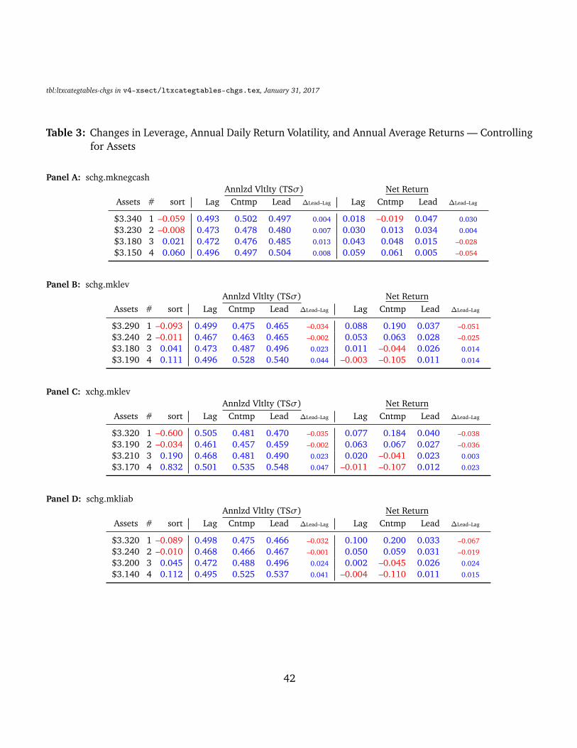
Table 3: Changes in Leverage, Annual Daily Return Volatility, and Annual Average Returns — Controllingfor Assets

tbl:ltxcategtables-chgs in v4-xsect/ltxcategtables-chgs.tex, January 31, 2017

Panel A: schg.mknegcashAnnlzd Vltlty (TSσ) Net Return

Assets # sort Lag Cntmp Lead ∆Lead–Lag Lag Cntmp Lead ∆Lead–Lag

$3.340 1 –0.059 0.493 0.502 0.497 0.004 0.018 –0.019 0.047 0.030

$3.230 2 –0.008 0.473 0.478 0.480 0.007 0.030 0.013 0.034 0.004

$3.180 3 0.021 0.472 0.476 0.485 0.013 0.043 0.048 0.015 –0.028

$3.150 4 0.060 0.496 0.497 0.504 0.008 0.059 0.061 0.005 –0.054

Panel B: schg.mklevAnnlzd Vltlty (TSσ) Net Return

Assets # sort Lag Cntmp Lead ∆Lead–Lag Lag Cntmp Lead ∆Lead–Lag

$3.290 1 –0.093 0.499 0.475 0.465 –0.034 0.088 0.190 0.037 –0.051

$3.240 2 –0.011 0.467 0.463 0.465 –0.002 0.053 0.063 0.028 –0.025

$3.180 3 0.041 0.473 0.487 0.496 0.023 0.011 –0.044 0.026 0.014

$3.190 4 0.111 0.496 0.528 0.540 0.044 –0.003 –0.105 0.011 0.014

Panel C: xchg.mklevAnnlzd Vltlty (TSσ) Net Return

Assets # sort Lag Cntmp Lead ∆Lead–Lag Lag Cntmp Lead ∆Lead–Lag

$3.320 1 –0.600 0.505 0.481 0.470 –0.035 0.077 0.184 0.040 –0.038

$3.190 2 –0.034 0.461 0.457 0.459 –0.002 0.063 0.067 0.027 –0.036

$3.210 3 0.190 0.468 0.481 0.490 0.023 0.020 –0.041 0.023 0.003

$3.170 4 0.832 0.501 0.535 0.548 0.047 –0.011 –0.107 0.012 0.023

Panel D: schg.mkliabAnnlzd Vltlty (TSσ) Net Return

Assets # sort Lag Cntmp Lead ∆Lead–Lag Lag Cntmp Lead ∆Lead–Lag

$3.320 1 –0.089 0.498 0.475 0.466 –0.032 0.100 0.200 0.033 –0.067

$3.240 2 –0.010 0.468 0.466 0.467 –0.001 0.050 0.059 0.031 –0.019

$3.200 3 0.045 0.472 0.488 0.496 0.024 0.002 –0.045 0.026 0.024

$3.140 4 0.112 0.495 0.525 0.537 0.041 –0.004 –0.110 0.011 0.015

42

(Table 3 continued)

Panel E: schg.bknegcashAnnlzd Vltlty (TSσ) Net Return

Assets # sort Lag Cntmp Lead ∆Lead–Lag Lag Cntmp Lead ∆Lead–Lag

$3.340 1 –0.061 0.490 0.489 0.483 –0.007 0.055 0.074 0.037 –0.018

$3.230 2 –0.008 0.477 0.482 0.484 0.006 0.015 0.034 0.038 0.022

$3.180 3 0.025 0.475 0.482 0.491 0.016 0.025 0.007 0.021 –0.004

$3.150 4 0.070 0.492 0.501 0.508 0.016 0.054 –0.012 0.005 –0.048

Panel F: schg.bklevAnnlzd Vltlty (TSσ) Net Return

Assets # sort Lag Cntmp Lead ∆Lead–Lag Lag Cntmp Lead ∆Lead–Lag

$3.270 1 –0.089 0.491 0.478 0.473 –0.018 0.085 0.107 0.041 –0.044

$3.280 2 –0.011 0.468 0.467 0.467 –0.001 0.043 0.047 0.032 –0.012

$3.230 3 0.037 0.475 0.488 0.493 0.018 0.009 –0.009 0.026 0.017

$3.120 4 0.109 0.499 0.521 0.532 0.033 0.011 –0.043 0.003 –0.009

Panel G: xchg.bklevAnnlzd Vltlty (TSσ) Net Return

Assets # sort Lag Cntmp Lead ∆Lead–Lag Lag Cntmp Lead ∆Lead–Lag

$3.280 1 –0.750 0.497 0.483 0.478 –0.018 0.079 0.107 0.042 –0.037

$3.230 2 –0.027 0.463 0.460 0.461 –0.002 0.049 0.049 0.030 –0.019

$3.240 3 0.204 0.471 0.483 0.489 0.017 0.014 –0.007 0.024 0.011

$3.150 4 1.140 0.503 0.527 0.539 0.035 0.006 –0.046 0.004 –0.002

Panel H: schg.bkliabAnnlzd Vltlty (TSσ) Net Return

Assets # sort Lag Cntmp Lead ∆Lead–Lag Lag Cntmp Lead ∆Lead–Lag

$3.300 1 –0.081 0.490 0.476 0.471 –0.019 0.087 0.096 0.036 –0.050

$3.260 2 –0.009 0.471 0.472 0.473 0.003 0.032 0.043 0.037 0.006

$3.180 3 0.039 0.476 0.488 0.494 0.017 0.010 –0.002 0.023 0.012

$3.160 4 0.102 0.497 0.518 0.528 0.030 0.020 –0.033 0.004 –0.016

Explanations: Variables and quartiles are explained in Table 1. The first column shows average book assets,intended to be held constant. The third column shows the sort criterion (identified in the panel header), intendedto be spread. The next four columns describe annual (fiscal-year) statistics for average daily stock-return volatility,during the year. Stock returns are always own returns minus the value-weighted stock-market return. The sortitself occurs at the end of the “Cntmp” period (and uses the Lag debt ratio to calculate the change). The deltacolumn highlights the return changes between lag and lead. The next four columns describe annualized excessreturns. Not reported, simple T-statistics for the differences between #4 and #1 in the “Lead” columns are allhighly statistically significant, permitting focus on economic rather than statistical significance.

Interpretation: Except for schg.mnknegcash, stocks with increasing leverage have subsequently higher volatility.Stocks with increasing leverage have subsequently lower average returns.

43

Table 4: Changes in Leverage, Annual Daily Return Volatility, and Annual Average Returns — Controllingfor Lag Returns

tbl:ltxcategtables-chgs-rc in v4-xsect/ltxcategtables-chgs.tex, January 31, 2017

Panel A: schg.mknegcashAnnlzd Vltlty (TSσ) Net Return

Assets # sort Lag Cntmp Lead ∆Lead–Lag Lag Cntmp Lead ∆Lead–Lag

$3.180 1 –0.058 0.492 0.497 0.492 0.000 0.038 –0.017 0.045 0.007

$3.620 2 –0.009 0.458 0.464 0.466 0.007 0.038 0.018 0.031 –0.007

$3.840 3 0.019 0.468 0.472 0.478 0.010 0.038 0.046 0.018 –0.020

$2.270 4 0.061 0.514 0.520 0.529 0.014 0.038 0.056 0.007 –0.031

Panel B: schg.mklevAnnlzd Vltlty (TSσ) Net Return

Assets # sort Lag Cntmp Lead ∆Lead–Lag Lag Cntmp Lead ∆Lead–Lag

$3.580 1 –0.088 0.497 0.479 0.469 –0.028 0.038 0.181 0.040 0.002

$3.260 2 –0.011 0.468 0.464 0.465 –0.003 0.038 0.056 0.025 –0.013

$3.120 3 0.041 0.469 0.484 0.490 0.020 0.038 –0.038 0.025 –0.013

$2.950 4 0.106 0.498 0.525 0.541 0.043 0.038 –0.097 0.011 –0.027

Panel C: xchg.mklevAnnlzd Vltlty (TSσ) Net Return

Assets # sort Lag Cntmp Lead ∆Lead–Lag Lag Cntmp Lead ∆Lead–Lag

$4.080 1 –0.569 0.499 0.480 0.470 –0.028 0.038 0.173 0.042 0.004

$2.750 2 –0.027 0.466 0.463 0.463 –0.004 0.038 0.062 0.023 –0.015

$2.750 3 0.239 0.468 0.482 0.488 0.021 0.038 –0.034 0.022 –0.016

$3.340 4 0.716 0.500 0.528 0.544 0.044 0.038 –0.097 0.014 –0.024

Panel D: schg.mkliabAnnlzd Vltlty (TSσ) Net Return

Assets # sort Lag Cntmp Lead ∆Lead–Lag Lag Cntmp Lead ∆Lead–Lag

$3.150 1 –0.084 0.500 0.482 0.475 –0.025 0.038 0.195 0.035 –0.004

$3.760 2 –0.011 0.465 0.462 0.462 –0.003 0.038 0.056 0.034 –0.004

$3.540 3 0.045 0.467 0.479 0.487 0.020 0.038 –0.045 0.021 –0.017

$2.460 4 0.107 0.501 0.529 0.542 0.041 0.038 –0.103 0.011 –0.026

44

(Table 4 continued)

Panel E: schg.bknegcashAnnlzd Vltlty (TSσ) Net Return

Assets # sort Lag Cntmp Lead ∆Lead–Lag Lag Cntmp Lead ∆Lead–Lag

$3.140 1 –0.059 0.491 0.489 0.483 –0.008 0.038 0.077 0.035 –0.003

$3.970 2 –0.008 0.463 0.466 0.469 0.006 0.038 0.033 0.033 –0.006

$3.350 3 0.024 0.470 0.477 0.483 0.013 0.038 0.008 0.026 –0.012

$2.450 4 0.069 0.509 0.519 0.530 0.021 0.038 –0.015 0.007 –0.030

Panel F: schg.bklevAnnlzd Vltlty (TSσ) Net Return

Assets # sort Lag Cntmp Lead ∆Lead–Lag Lag Cntmp Lead ∆Lead–Lag

$3.660 1 –0.086 0.489 0.478 0.474 –0.015 0.038 0.105 0.041 0.003

$3.280 2 –0.012 0.470 0.468 0.468 –0.002 0.038 0.045 0.029 –0.009

$3.070 3 0.037 0.474 0.486 0.491 0.017 0.038 –0.009 0.026 –0.012

$2.900 4 0.105 0.500 0.520 0.533 0.033 0.038 –0.039 0.005 –0.033

Panel G: xchg.bklevAnnlzd Vltlty (TSσ) Net Return

Assets # sort Lag Cntmp Lead ∆Lead–Lag Lag Cntmp Lead ∆Lead–Lag

$4.100 1 –0.721 0.489 0.478 0.475 –0.015 0.038 0.101 0.039 0.001

$2.900 2 –0.016 0.469 0.468 0.467 –0.002 0.038 0.048 0.030 –0.008

$2.670 3 0.270 0.474 0.485 0.489 0.015 0.038 –0.006 0.024 –0.014

$3.240 4 1.007 0.501 0.521 0.534 0.034 0.038 –0.040 0.008 –0.030

Panel H: schg.bkliabAnnlzd Vltlty (TSσ) Net Return

Assets # sort Lag Cntmp Lead ∆Lead–Lag Lag Cntmp Lead ∆Lead–Lag

$3.170 1 –0.077 0.491 0.481 0.476 –0.015 0.038 0.095 0.037 –0.001

$3.900 2 –0.010 0.467 0.466 0.468 0.001 0.038 0.041 0.035 –0.003

$3.510 3 0.039 0.471 0.481 0.486 0.016 0.038 –0.004 0.022 –0.016

$2.330 4 0.100 0.504 0.523 0.535 0.031 0.038 –0.030 0.006 –0.031

Explanations: This table is identical to the previous one, except that quartiles are now sorted to control for the lag net return(instead of sorted to control for assets).

Interpretation: Firms increasing leverage are experiencing declines in average net returns.

45

Table 5: Annual Stock Return Characteristics Surrounding Changes in Debt Ratios

tbl:ltxregtables-schgs in v4-xsect/ltxregtables-schgs.tex, January 31, 2017

Panel A: Regression Coefficients Explaining Lead Daily Non-Annualized Volatility (SD) With Own Lag and (Reported)Change in Leverage Ratio

Fama-Macbeth Panel RegressionsCoef (T-NW) Coef (T-DC)

schg.mknegcash 0.002 (2.77) –0.001 (−0.52)schg.mklev 0.019 (8.30) 0.023 (13.34)schg.mkliab 0.021 (7.80) 0.025 (13.83)

schg.bknegcash 0.010 (8.29) 0.012 (11.88)schg.bklev 0.013 (9.41) 0.014 (14.82)schg.bkliab 0.015 (8.90) 0.017 (16.06)

Panel B: Regression Coefficients Explaining Lead Daily Average Annual Returns With Own Lag and (Reported)Change in Leverage Ratio

Fama-Macbeth Panel RegressionsCoef (T-NW) Coef (T-DC)

schg.mknegcash –0.230 (−4.07) –0.316 (−3.71)schg.mklev –0.069 (−1.08) –0.048 (−0.56)schg.mkliab –0.042 (−0.62) –0.007 (−0.08)

schg.bknegcash –0.123 (−2.49) –0.080 (−2.27)schg.bklev –0.107 (−2.13) –0.087 (−1.91)schg.bkliab –0.091 (−1.58) –0.054 (−1.19)

Explanations: The regressions use the same annual data as the previous “category” Table 3. Let R y be eitherthe the average daily equity return (net of the market) volatility over year y in Panel A, or the compound return(net of the market) in panel B; and let L y be the leverage measure at the end of the year. The regression isRt+1 = a+ b · Rt−1 + c · (Lt − Lt−1) + e. It is the coefficient c that is reported in the two panels. The coefficientsin the second column are from Fama-Macbeth regressions (albeit on annual returns), with T-statistics based on3 Newey-West lags in the third column. The coefficients in the fourth column are from OLS regressions, withdouble-clustered and White heterogeneity-adjusted T-statistics in the fifth column.

Interpretation: Except for schg.mknegcash, which is unrelated, volatility increases with leverage. Annual returnsare too weak to be predicted reliably, but the sign is usually negative and some specifications are significant.

46

Table 6: The Effect of Changes in Debt Ratios on Subsequent Monthly Stock Returns, All Stocks

tbl:famatables-schgs in v4-xsect/famatables-schgs.tex, January 31, 2017

Panel A: Fama-French Alphas for Quartile Portfolios Spread By Debt-Ratio Changes, Year and Book-Asset Balanced

Raw XMKT XMKT,SMB,HMLXMKT,SMB,HML,

RMW,CMAXMKT,SMB,HML,RMW,CMA,UMD

Alpha (T-stat) Alpha (T-stat) Alpha (T-stat) Alpha (T-stat) Alpha (T-stat)

schg.mknegcash –0.334 (−7.15) –0.357 (−7.73) –0.312 (−7.02) –0.252 (−5.68) –0.253 (−5.62)schg.mklev –0.230 (−3.16) –0.272 (−3.81) –0.366 (−5.39) –0.262 (−3.88) –0.097 (−1.72)schg.mkliab –0.208 (−2.84) –0.246 (−3.40) –0.343 (−4.99) –0.242 (−3.54) –0.076 (−1.33)

schg.bknegcash –0.261 (−5.98) –0.287 (−6.70) –0.274 (−6.55) –0.200 (−4.89) –0.155 (−3.86)schg.bklev –0.325 (−5.90) –0.365 (−6.85) –0.395 (−7.56) –0.294 (−5.82) –0.201 (−4.34)schg.bkliab –0.285 (−5.56) –0.323 (−6.52) –0.348 (−7.23) –0.265 (−5.59) –0.181 (−4.13)

Panel B: Fama-Macbeth Regressions, Coefficient Reported Only For Key Debt Measure

Solo Solo Incl. Cntrls Incl. Cntrls (TSσ)DT Qrtl (T-stat) DT Ratio (T-stat) DT Ratio (T-stat) DT Ratio (T-stat)

schg.mknegcash –0.077 (−4.56) –1.869 (−4.70) –1.636 (−4.33) –1.678 (−4.55)schg.mklev –0.080 (−3.04) –1.332 (−4.48) –0.550 (−2.28) –0.472 (−1.99)schg.mkliab –0.078 (−3.43) –1.106 (−3.27) –0.164 (−0.63) –0.046 (−0.18)

schg.bknegcash –0.075 (−6.79) –1.333 (−3.93) –0.911 (−2.54) –0.885 (−2.46)schg.bklev –0.106 (−5.42) –1.435 (−7.06) –0.528 (−2.79) –0.482 (−2.55)schg.bkliab –0.106 (−8.02) –1.372 (−5.64) –0.421 (−2.06) –0.360 (−1.79)

Explanations: The content and format of these tables is identical to those in Table 2, except that the variable underconsideration is now the simple change in the leverage ratios. All stock returns are measured after the increase inleverage, with a 4-5 months accounting lag.

Interpretation: Firms that increased leverage had lower subsequent average rates of return. The magnitude andsignificance depends on the controls.

47

Table 7: The Effect of Changes in Market-Based Debt Ratios on Subsequent Monthly Stock Returns,Cross-Classified Simultaneous Risk (Daily Volatility and Market-Beta) Changes

tbl:xtables-bysigma in v4-xsect/xtables-bysigma.tex, January 31, 2017

schg.mknegcash schg.mklev schg.mkliab

Firm

Year

s∆

Tota

lAnn

lzd

Eqty

Vola

tilit

yA

nnua

lA

vgR

etur

ns

Lev Risk ↓ unclr Risk ↑

1↓ 16,904 4,738 16,1802 16,919 5,134 15,7693 16,866 5,057 15,8774↑ 17,334 4,834 15,632

Lev Risk ↓ unclr Risk ↑

1↓ –0.121 0.021 0.1392 –0.108 0.023 0.1373 –0.105 0.029 0.1434↑ –0.111 0.025 0.150

Lev Risk ↓ unclr Risk ↑

1↓ 0.038 0.034 0.0622 0.035 0.013 0.0393 0.022 0.001 0.0134↑ 0.008 –0.004 0.003

Lev Risk ↓ unclr Risk ↑

1↓ 18,743 4,957 14,1222 17,473 5,147 15,2023 16,276 5,088 16,4364↑ 15,531 4,571 17,698

Lev Risk ↓ unclr Risk ↑

1↓ –0.140 0.015 0.0962 –0.108 0.023 0.1183 –0.097 0.027 0.1564↑ –0.095 0.034 0.188

Lev Risk ↓ unclr Risk ↑

1↓ 0.040 0.028 0.0362 0.030 0.014 0.0303 0.026 0.003 0.0324↑ 0.004 –0.005 0.021

Lev Risk ↓ unclr Risk ↑

1↓ 18,759 4,888 14,1752 17,458 5,246 15,1183 16,217 5,048 16,5354↑ 15,589 4,581 17,630

Lev Risk ↓ unclr Risk ↑

1↓ –0.138 0.020 0.0962 –0.109 0.020 0.1233 –0.097 0.027 0.1564↑ –0.095 0.031 0.184

Lev Risk ↓ unclr Risk ↑

1↓ 0.033 0.026 0.0362 0.035 0.007 0.0353 0.026 0.009 0.0314↑ 0.006 –0.001 0.018

schg.bknegcash schg.bklev schg.bkliab

Firm

Year

s∆

Tota

lAnn

lzd

Eqty

Vola

tilit

yA

nnua

lA

vgR

etur

ns

Lev Risk ↓ unclr Risk ↑

1↓ 17,525 4,911 15,3862 16,878 5,040 15,9043 16,772 5,060 15,9684↑ 16,848 4,752 16,200

Lev Risk ↓ unclr Risk ↑

1↓ –0.124 0.020 0.1262 –0.112 0.024 0.1383 –0.103 0.027 0.1524↑ –0.104 0.027 0.153

Lev Risk ↓ unclr Risk ↑

1↓ 0.030 0.024 0.0512 0.034 0.024 0.0463 0.032 0.000 0.0164↑ 0.007 –0.007 0.007

Lev Risk ↓ unclr Risk ↑

1↓ 18,151 4,929 14,7422 17,296 5,120 15,4063 16,521 5,085 16,1944↑ 16,055 4,629 17,116

Lev Risk ↓ unclr Risk ↑

1↓ –0.129 0.020 0.1112 –0.110 0.022 0.1213 –0.102 0.025 0.1534↑ –0.101 0.032 0.179

Lev Risk ↓ unclr Risk ↑

1↓ 0.038 0.031 0.0472 0.031 0.018 0.0373 0.028 0.005 0.0314↑ 0.005 –0.014 0.005

Lev Risk ↓ unclr Risk ↑

1↓ 18,279 4,910 14,6332 17,158 5,125 15,5393 16,533 5,049 16,2184↑ 16,053 4,679 17,068

Lev Risk ↓ unclr Risk ↑

1↓ –0.128 0.019 0.1102 –0.109 0.022 0.1283 –0.104 0.027 0.1534↑ –0.101 0.030 0.173

Lev Risk ↓ unclr Risk ↑

1↓ 0.033 0.024 0.0442 0.035 0.019 0.0463 0.028 0.008 0.0224↑ 0.005 –0.011 0.008

48

(Table 7 continued)

Explanations: “Risk ↑” (“Risk ↓”) stocks are those that experienced both a daily equity volatility increase(decrease) of at least 0.1%/day (1.6% per annum) from the lag year (–1,0) to the lead year (0,+1).Displayed volatilities and returns are for year (+1,+2). The leverage quartiles are the same four schgcategories as those used elsewhere in the paper. The displayed post-sort monthly average returns andpost-sort total volatility changes are measured monthly over the 12 months following the leverage andstock risk changes.

Interpretation: The cash-change leverage ratios, mknegcash and bknegcash, show only weak changes insubsequent equity volatility, but the two broader leverage metrics show clear volatility increases. Leverageassociates with lower subsequent average returns for all leverage metrics, even for stocks with increasingrisk.

49

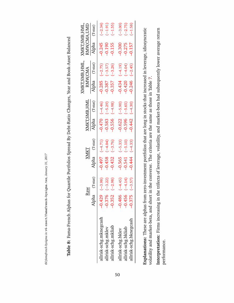
Tabl

e8:

Fam

a-Fr

ench

Alp

has

for

Qua

rtile

Port

folio

sSp

read

By

Deb

t-R

atio

Cha

nges

,Yea

ran

dB

ook-

Ass

etB

alan

ced

tbl:f

amaf

renc

h-by

sigm

ainv4

-xse

ct/f

amaf

renc

h-by

sigm

a.te

x,Ja

nuar

y31

,201

7

Raw

XM

KT

XM

KT,

SMB

,HM

LX

MK

T,SM

B,H

ML,

RM

W,C

MA

XM

KT,

SMB

,HM

L,R

MW

,CM

A,U

MD

Alp

ha(T

-sta

t)A

lpha

(T-s

tat)

Alp

ha(T

-sta

t)A

lpha

(T-s

tat)

Alp

ha(T

-sta

t)

allr

isk-

schg

.mkn

egca

sh–0

.429

(−3.

98)

–0.4

97(−

4.71)

–0.4

70(−

4.46)

–0.2

85(−

2.75)

–0.2

45(−

2.34)

allr

isk-

schg

.mkl

ev–0

.376

(−3.

22)

–0.4

58(−

4.04)

–0.5

83(−

5.29)

–0.3

87(−

3.57)

–0.1

90(−

1.91)

allr

isk-

schg

.mkl

iab

–0.3

52(−

2.98)

–0.4

32(−

3.76)

–0.5

56(−

4.98)

–0.3

57(−

3.26)

–0.1

55(−

1.55)

allr

isk-

schg

.bkl

ev–0

.486

(−4.

45)

–0.5

65(−

5.33)

–0.6

22(−

5.90)

–0.4

34(−

4.19)

–0.3

00(−

3.00)

allr

isk-

schg

.bkl

iab

–0.4

56(−

4.14)

–0.5

41(−

5.10)

–0.5

96(−

5.65)

–0.4

20(−

4.04)

–0.2

75(−

2.75)

allr

isk-

schg

.bkn

egca

sh–0

.375

(−3.

57)

–0.4

44(−

4.33)

–0.4

42(−

4.30)

–0.2

46(−

2.45)

–0.1

57(−

1.58)

Expl

anat

ion

s:Th

ese

are

alph

asfr

omze

ro-in

vest

men

tpor

tfol

ios

that

are

long

inst

ocks

that

incr

ease

din

leve

rage

,idi

osyn

crat

icvo

lati

lity

and

mar

ket-

beta

,and

shor

tin

the

conv

erse

.Th

ecr

iter

iaar

eth

esa

me

asth

ose

inTa

ble

7.

Inte

rpre

tati

on:

Firm

sin

crea

sing

inth

etr

ifect

aof

leve

rage

,vol

atili

ty,a

ndm

arke

t-be

taha

dsu

bseq

uent

lylo

wer

aver

age

retu

rnpe

rfor

man

ce.

50

Table 9: The Effect of Changes in Stock-Implied Not-Firm-Managed Changes in Debt Ratios on SubsequentMonthly Stock Returns

tbl:famatables-ivs in v4-xsect/famatables-ivs.tex, January 31, 2017

Panel A: Fama-French Alphas for Quartile Portfolios Spread By Instrumented Debt-Ratio Changes, Yearand Book-Asset Balanced

Raw XMKT XMKT,SMB,HMLXMKT,SMB,HML,

RMW,CMAAlpha (T-stat) Alpha (T-stat) Alpha (T-stat) Alpha (T-stat)

R.schg.mklev –0.241 (−2.45) –0.306 (−3.19) –0.413 (−4.49) –0.274 (−2.99)R.schg.mkliab –0.261 (−2.48) –0.324 (−3.13) –0.452 (−4.57) –0.308 (−3.12)

Panel B: Fama-Macbeth Regressions, Coefficient Reported Only For (Instrumented) Key Variables

Solo Solo Incl. Cntrls Incl. Cntrls (TSσ)DT Qrtl (T-stat) DT Ratio (T-stat) DT Ratio (T-stat) DT Ratio (T-stat)

R.schg.mklev –0.109 (−3.36) –4.009 (−5.36) –1.545 (−2.68) –1.438 (−2.52)R.schg.mkliab –0.118 (−3.70) –3.370 (−4.76) –1.052 (−1.66) –0.900 (−1.43)

Explanations: The indebtedness variable is not the leverage at the end of the year, but the leverageat the beginning of the year grossed up by the firm’s rate of return. Thus, these leverage changes arewithout active managerial leverage changes instituted during the year. Any stock-return based shock toleverage would therefore not have (yet) been counteracted by managerial capital structure policy.

Interpretation: Even for leverage changes that are not actively set by corporate management, leveragechanges have the same negative influence on subsequent average returns.

51

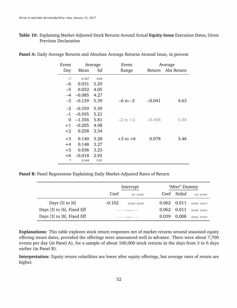
Table 10: Explaining Market-Adjusted Stock Returns Around Actual Equity-Issue Execution Dates, GivenPrevious Declaration

tbl:sdc in welch4-divstudytbls.tex, January 31, 2017

Panel A: Daily Average Returns and Absolute Average Returns Around Issue, in percent

Event Average Event AverageDay Mean Sd Range Return Abs Return

–7 0.167 4.04

–6 0.031 5.29–5 0.032 4.05–4 –0.085 4.27–3 –0.139 5.39 –6 to –3 –0.041 4.63

–2 –0.359 5.39–1 –0.595 5.210 –1.356 5.81 –2 to +2 –0.448 5.04+1 –0.205 4.98+2 0.258 3.34

+3 0.140 3.28 +3 to +6 0.078 3.46+4 0.148 3.27+5 0.036 3.23+6 –0.018 2.95

7 0.164 3.01

Panel B: Panel Regressions Explaining Daily Market-Adjusted Rates of Return

Intercept “After”-Dummy

Coef (se) (se.het) Coef Stdzd (se) (se-het)

Days |3| to |6| –0.162 (0.014) (0.014) 0.062 0.011 (0.018) (0.017)

Days |3| to |6|, Fixed Eff ———— many ——— 0.062 0.011 (0.018) (0.015)

Days |3| to |8|, Fixed Eff ———— many ——— 0.039 0.008 (0.015) (0.015)

Explanations: This table explores stock return responses net of market returns around seasoned equityoffering issues dates, provided the offerings were announced well in advance. There were about 7,700events per day (in Panel A), for a sample of about 100,000 stock returns in the days from 3 to 6 daysearlier (in Panel B).

Interpretation: Equity return volatilities are lower after equity offerings, but average rates of return arehigher.

52

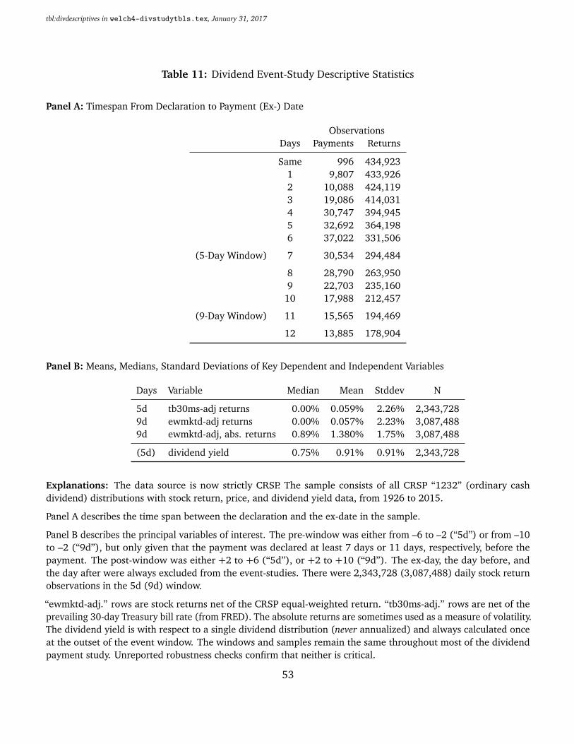
Table 11: Dividend Event-Study Descriptive Statistics

tbl:divdescriptives in welch4-divstudytbls.tex, January 31, 2017

Panel A: Timespan From Declaration to Payment (Ex-) Date

ObservationsDays Payments Returns

Same 996 434,9231 9,807 433,9262 10,088 424,1193 19,086 414,0314 30,747 394,9455 32,692 364,1986 37,022 331,506

(5-Day Window) 7 30,534 294,484

8 28,790 263,9509 22,703 235,16010 17,988 212,457

(9-Day Window) 11 15,565 194,469

12 13,885 178,904

Panel B: Means, Medians, Standard Deviations of Key Dependent and Independent Variables

Days Variable Median Mean Stddev N

5d tb30ms-adj returns 0.00% 0.059% 2.26% 2,343,7289d ewmktd-adj returns 0.00% 0.057% 2.23% 3,087,4889d ewmktd-adj, abs. returns 0.89% 1.380% 1.75% 3,087,488

(5d) dividend yield 0.75% 0.91% 0.91% 2,343,728

Explanations: The data source is now strictly CRSP. The sample consists of all CRSP “1232” (ordinary cashdividend) distributions with stock return, price, and dividend yield data, from 1926 to 2015.

Panel A describes the time span between the declaration and the ex-date in the sample.

Panel B describes the principal variables of interest. The pre-window was either from –6 to –2 (“5d”) or from –10to –2 (“9d”), but only given that the payment was declared at least 7 days or 11 days, respectively, before thepayment. The post-window was either +2 to +6 (“5d”), or +2 to +10 (“9d”). The ex-day, the day before, andthe day after were always excluded from the event-studies. There were 2,343,728 (3,087,488) daily stock returnobservations in the 5d (9d) window.

“ewmktd-adj.” rows are stock returns net of the CRSP equal-weighted return. “tb30ms-adj.” rows are net of theprevailing 30-day Treasury bill rate (from FRED). The absolute returns are sometimes used as a measure of volatility.The dividend yield is with respect to a single dividend distribution (never annualized) and always calculated onceat the outset of the event window. The windows and samples remain the same throughout most of the dividendpayment study. Unreported robustness checks confirm that neither is critical.

53

Table 12: Risk and Reward Changes Around Dividend Cum-Ex Transitions

tbl:divriskreward in welch4-divstudytbls.tex, January 31, 2017

Panel A: Risk Measures“After-Dividend “Win-Start Cross-

Intercept Dummy” Div Yield” Coefficient

Coef Coef Stdzd Coef Stdzd Coef Stdzd

A.1 5d, tb30ms-adj, SD(R) 1.711 0.010 0.003A.2 9d, ewmktd-adj, ABS(R), Evt FE many 0.014 0.005

A.3 1992- 5d, ewmktd-adj, wins 1.353 0.020 0.006

A.4 By divyield, SD(R), 5d, ewmkt, wins incl 0.000 0.000 –1.385 –0.009 1.386 0.008A.5 same, but 1992- incl 0.009 0.000 2.226 0.015 1.432 0.008

Panel B: Reward Measures“After-Dividend “Win-Start Cross-

Intercept Dummy” Div Yield” Coefficient

Coef Coef Stdzd Coef Stdzd Coef Stdzd

B.1 5d, risk-free-adj 0.076 –0.035 –0.008B.2 9d, ewmkt-adj, Evt FE many –0.030 –0.008

B.3 1992- 5d, ewmkt, Wnsr, –0.003 –0.050 –0.012

B.4 By Div Yield, 5d, ewmkt, Wnsr incl –0.001 0.000 3.116 0.014 –6.137 –0.023B.5 Same, 1992- incl –0.002 –0.001 2.737 0.014 –5.932 –0.024

Explanations: Samples and variables are described in Table 11. Each line contains the coefficients of one panelregression. The “after-dividend” dummy is 0 for days from −T to −2 (inclusive) and 1 for days from 2 to T(inclusive). Other days were excluded. The dividend declaration must have occurred at least two days before thestart of the window. The standard errors, even using many corrections, are so low (given the gigantic number ofobservations) that the reader can focus on the coefficient magnitudes. The column labeled “Stdzd” coefficient isthe plain coefficient multiplied by sd(x)/sd(y). The risk measures are either the standard deviation (SD(R)) or theabsolute value (ABS(R)). When the regressors include the dividend-yield at the start of the event-window, theyalso contain the “cross”-variable, i.e., the Dividend Yield times the “After Dividend” Dummy. When winsorization(Wnsr) was applied, it was for daily returns at +20% and –20%.

Interpretation: (A.1-A.3) The volatility after the dividend payment was higher, by about 1 bp per day. (A.4-A.5)The volatility after the dividend payment was higher for higher-dividend yield events. (B.1-B.3) The average rateof return after the dividend payment was lower by about 2-5 bp per day. With 4-8 day windows, this amountsto about 20-30 bp over the full windows. (B.4-B.5) Only the cross-effect mattered. Firms paying more dividendsappreciated more at the payment and then delivered lower returns thereafter. The dividend payment reduced theaverage daily rate of return by about 3bp for every 1% dividend yield. Over 4-8 day windows, this amounts toabout 20-30bp.

54

Figure 1: Effects of Pre-Announced Dividend Payments on Absolute Rates of Return

fig:divvols in welch4-divstudytbls.tex, January 31, 2017

ε to 1% Dividend 1% to 2% Dividend

−20 −10 0 10 20

1.25

1.30

1.35

1.40

Event Day

Mean N

et

Abs

RR ●●●●●●

●

●

●

●

●

●●

●

●

●

●

●

●●

●●●●●●

●

●

●

●

●

●

●

●

●

●

●

●●

●

div

yld

= 0

.005;

1/(

1−

div

yld

)= 1

.005

−20 −10 0 10 20

1.24

1.26

1.28

1.30

1.32

Event Day

Mean N

et

Abs

RR

●●●●●●

●

●

●

●

●

●

●●●

●●●●

●

●●●●●●

●

●

●

●

●

●●

●

●●

●●

●

●

div

yld

= 0

.014;

1/(

1−

div

yld

)= 1

.014

More than 2% Dividend All Dividend Events

−20 −10 0 10 20

1.25

1.30

1.35

1.40

Event Day

Mean N

et

Abs

RR

●●●●●●

●●

●

●

●●

●

●●●●●●

●

●●●●●●

●

●

●●●●

●

●

●●

●●●●

div

yld

= 0

.026;

1/(

1−

div

yld

)= 1

.027

−20 −10 0 10 20

1.26

1.28

1.30

1.32

1.34

1.36

1.38

Event Day

Mean N

et

Abs

RR

●●●●●●

●

●

●

●●

●●●

●

●●

●

●●

●●●●●●

●

●

●

●●

●●

●●

●

●●

●

●

div

yld

= 0

.009;

1/(

1−

div

yld

)= 1

.009

Explanations: Samples and variables are described in Table 11. The four plots are, in clockwise order,averages of absolute net-of-market rates of return for low-yield, mid-yield, high-yield (less than 1%,1-2%, and more than 3%), and all dividend payments . The four solid lines represent all the stocks whichhave at least 5, 10, 15, or 20 trading days around the payment date. Thus, the gray line has the fewestnumber of stocks, but extends farthest. The dashed line mixes in all stock returns without requiring aconstant set of firms.

Interpretation: Post-payment volatilities were higher than pre-payment volatilities, but only reliablyso for high-yield dividend events. The selection window influences the reported volatilities, but onlymoderately so. Even the selection-unconditional mix of firms produces roughly the same inference.

55

Figure 2: Effects of Pre-Announced Dividend Payments on Average Rates of Return

fig:divmeans in welch4-divstudytbls.tex, January 31, 2017

ε to 1% Dividend 1% to 2% Dividend

−20 −10 0 10 20

−0.04

−0.03

−0.02

−0.01

0.00

0.01

0.02

Event Day

Mean N

et

RR

●●●●●●●

●●●●

●●●●

●●●●●

●●●●●●

●

●●●●●●●●●●●●●

div

yld

= 0

.005;

1/(

1−

div

yld

)= 1

.005

−20 −10 0 10 20

−0.05

0.00

0.05

0.10

Event Day

Mean N

et

RR

●●●●●●

●

●●●

●●●●●●●●●●

●●●●●●●●●●●●

●

●

●●●

●●●

div

yld

= 0

.014;

1/(

1−

div

yld

)= 1

.014

More than 2% Dividend All Dividend Events

−20 −10 0 10 20

−0.2

−0.1

0.0

0.1

0.2

Event Day

Mean N

et

RR

●●●●●●●●●

●●●●●●●●

●●●

●●●●●●

●

●●●

●●

●●●

●●●●

●

div

yld

= 0

.026;

1/(

1−

div

yld

)= 1

.027

−20 −10 0 10 20

−0.04

−0.02

0.00

0.02

0.04

0.06

Event Day

Mean N

et

RR

●●●●●●

●

●●●●●●●●●●●●●

●●●●●●

●●●●●●●●●●●●●●

div

yld

= 0

.009;

1/(

1−

div

yld

)= 1

.009

Explanations: Samples and variables are described in Table 11. The four plots are, in clockwise order,averages of absolute net-of-market rates of return for low-yield, mid-yield, high-yield (less than 1%,1-2%, and more than 3%), and all dividend payments. The four solid lines represent all the stocks whichhave at least 5, 10, 15, or 20 trading days around the payment date. Thus, the gray line has the fewestnumber of stocks, but extends farthest. The dashed line mixes in all stock returns without requiring thata constant set of firms.

Interpretation: Post-payment average returns were lower than pre-payment volatilities, and only reliablyso for higher-yield dividend events. The selection window influences the reported average returns, butonly moderately so. Even the selection-unconditional mix of firms produces roughly the same inference.The y-scale changes understate the visual impact of the effect.

56

Figure 3: Year-by-Year Coefficients Explaining Stock Return Moments after Payment and highest Individ-ual Dividend Income Tax Rates

fig:byyear in welch4-divstudytbls.tex, January 31, 2017

Panel A: Explaining Volatility (Absolute Return)

1960 1970 1980 1990 2000 2010

−0.02

0.00

0.02

0.04

0.06

0.08

0.10

0.12

Index

vols

coef

Panel B: Explaining Average (Returns)

1960 1970 1980 1990 2000 2010

−0.15

−0.10

−0.05

0.00

Index

avgs

coef

Panel C: Personal Income Tax Rate on Dividends by Year

1960 1970 1980 1990 2000 2010

0

20

40

60

80

100

Index

tax r

ate

Explanations: Samples and variables are described in Table 11. Panels A and B show the regression coefficients ofinterest (analogous to those in Table 12) when each year is run by itself for the market-adjusted 5-day window. Theblue lines in Panel A are for equity volatility: The solid blue line is on the “after-payment” dummy in a bivariateregression. The dashed blue line is on a multivariate regression for the “cross” variable. The red lines in Panel Bare for average returns: The solid red line is on a bivariate regression “after-payment” dummy. The dashed red lineis on a multivariate regression for the cross variable. To fit on the same scale, the cross-coefficients were divided by100. Panel C shows dividend tax rates, as in Sialm (2009), Becker, Jacob, and Jacob (2013), and Jacob, Michaely,and Mueller (2016).

Interpretation: The effects varied year-by-year, but have not changed in a systematic fashion. This also suggeststhat although there may have been contributions of personal dividend income tax-related preferences to thedividend-payment effect, tax effects could not have been too powerful.

57

Table 13: Different Types of Dividends

tbl:divbytype in welch4-divstudytbls.tex, January 31, 2017

Panel B: Controlling for Dividend Characteristics

Coefficients

Div Yield Bivariate Reg Multivariate Regression

δ After-Dummy After-Dummy δ Cross N

Taxable (code 2) 0.94% –0.017 –0.005 0.681 –1.321 9,985,317Nontaxable (code 3) 0.50% –0.011 0.060 6.249 –14.303 247,535

Recurring 0.88% –0.016 0.016 2.668 –3.724 10,105,183Special 4.14% –0.095 –0.090 –0.237 –0.154 139,922

Previous Dividend

0-75 days 0.84% –0.008 0.005 0.905 –1.603 871,62076-120 days 0.89% –0.016 0.027 3.507 –4.927 5,670,443121-200 days 0.87% –0.019 0.031 3.979 –5.812 1,151,275201-500 days 0.93% –0.022 0.008 2.281 –3.183 717,506New 0.97% –0.026 0.004 1.535 –3.061 210,975

Panel B: Controlling for Prevailing Liability Ratio

Coefficients

Liability Div Yield Bivariate Reg Multivariate Regression

Ratio δ After-Dummy After-Dummy δ Cross N

Low (0 < TL/TA < 1/3) 1.02% –0.024 –0.014 0.391 –1.001 1,892,293Medium (1/3 < TL/TA < 2/3) 0.96% –0.024 –0.009 0.868 –1.535 3,712,706High (2/3 < TL/TA < 3/3) 0.90% –0.008 0.004 0.783 –1.337 3,569,510

Explanations: Each line shows coefficients from two panel regressions, analogous to those in Table 12,but using the longest symmetric event window around the payment, and beginning two days after thepublic dividend declaration. Only ordinary dividends (CRSP distcd first digit 1) are used. In Panel A,taxability of dividends is identified in the fourth digit of the distcd. The classification between recurringand special dividends is identified in the second digit of the distcd (codes 2 through 5 for recurrent,7 for special). The length of time since the last paid dividend is calculated from the CRSP panel. AllOLS coefficients are highly statistically significant, except for two italicized entries for special dividends(which are only about 1% of the sample). In Panel B, stocks are classified by financial liabilities (the ratioof total liabilities net of cash divided by the book value of total assets), truncated at zero and one, in thecalendar year before the dividend declaration.

Interpretation: The mean rate of return after the payment is lower than the mean rate of return beforethe payment, regardless of whether the dividend was taxable or nontaxable, regular or irregular; andwhether the firm was modestly or highly indebted.

58

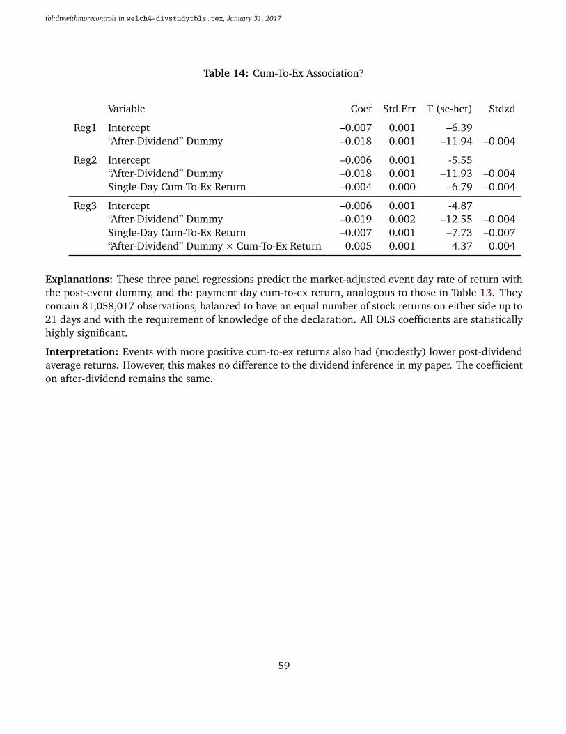
Table 14: Cum-To-Ex Association?

tbl:divwithmorecontrols in welch4-divstudytbls.tex, January 31, 2017

Variable Coef Std.Err T (se-het) Stdzd

Reg1 Intercept –0.007 0.001 –6.39“After-Dividend” Dummy –0.018 0.001 –11.94 –0.004

Reg2 Intercept –0.006 0.001 -5.55“After-Dividend” Dummy –0.018 0.001 –11.93 –0.004Single-Day Cum-To-Ex Return –0.004 0.000 –6.79 –0.004

Reg3 Intercept –0.006 0.001 -4.87“After-Dividend” Dummy –0.019 0.002 –12.55 –0.004Single-Day Cum-To-Ex Return –0.007 0.001 –7.73 –0.007“After-Dividend” Dummy × Cum-To-Ex Return 0.005 0.001 4.37 0.004

Explanations: These three panel regressions predict the market-adjusted event day rate of return withthe post-event dummy, and the payment day cum-to-ex return, analogous to those in Table 13. Theycontain 81,058,017 observations, balanced to have an equal number of stock returns on either side up to21 days and with the requirement of knowledge of the declaration. All OLS coefficients are statisticallyhighly significant.

Interpretation: Events with more positive cum-to-ex returns also had (modestly) lower post-dividendaverage returns. However, this makes no difference to the dividend inference in my paper. The coefficienton after-dividend remains the same.

59

Figure 4: Explaining Average Trading Liquidity Patterns around Previously Declared Payment Dates

fig:liquidity in welch4-divstudytbls.tex, January 31, 2017

−10 −5 0 5 10

0

5

10

15

Payment Evt Day

#

● ● ● ● ● ● ● ● ● ● ● ● ● ● ● ● ● ● ● ● ● ● ● ● ●Log Number of Trades

● ● ● ● ● ● ● ● ● ● ● ● ● ● ● ● ● ● ● ● ● ● ● ● ●Log Dollar Volume of Trades

Explanations: Samples and variables are described in Table 11. These are plots of the by-event-dayaverages of the log number of trades and log value of dollar trades.

Interpretation: Liquidity-related trading explanations are unlikely to play a role.

60

Tabl

e15

:Il

lust

rati

veN

umer

ical

Exam

ple

of(P

ost-

Ann

ounc

emen

t)A

t-Pa

ymen

tC

hang

es

tbl:i

llust

rate

inwe

lch4

-app

endi

xtbl

s.te

x,Ja

nuar

y31

,201

7

Firm

Low

Leve

rage

(D0=

$5,

E 0=

$95,δ=

1.05

%)

Hig

hLe

vera

ge(D

0=

$95,

E 0=

$5,δ=

20%

)

Ris

kyP

Safe

C$0

$100

NoRisk

[$10

0,$1

00]

Secu

rity

T=

0T=

2R

isk

@T

Deb

t(FV=

$5)

$5($

5,$5

)Eq

uity

Cum

T=

0.9

$95

($95

,$95

)±

0.00

%Eq

uity

ExT=

1.1

$94

($95

–$1,

95–$

1)±

0.00

%

Secu

rity

T=

0T=

2R

isk

@T

Deb

t(FV=

$95)

$95

($95

,$95

)Eq

uity

Cum

T=

0.9

$5($

5,$5

)±

0.00

%Eq

uity

ExT=

1.1

$94

($5–

$1,5

–$1)

±0.

00%

Ris

kyP

Safe

C$2

$98

LowRisk

[$99

.8,$

100.

2]

Secu

rity

T=

0T=

2R

isk

@T

Deb

t(FV=

$5)

$5($

5,$5

)Eq

uity

Cum

T=

0.9

$95

($94

.8,$

95.2

)±

0.21

0%Eq

uity

ExT=

1.1

$94

($94

.8–$

1,95

.2–$

1)±

0.21

3%

Secu

rity

T=

0T=

2R

isk

@T

Deb

t(FV=

$95)

$95

($95

,$95

)Eq

uity

Cum

T=

0.9

$5($

4.8,

$5.2

)±

4.0%

Equi

tyEx

T=

1.1

$94

($4.

8–$1

,5.2

–$1)

±5.

0%

Ris

kyP

Safe

C$9

8$2

HighRisk

[$90

.2,$

109.

8]

Secu

rity

T=

0T=

2R

isk

@T

Deb

t(FV=

$5)

$5($

5,$5

)Eq

uity

Cum

T=

0.9

$95

($85

.2,$

104.

8)±

10.3

2%Eq

uity

ExT=

1.1

$94

($85

.2–$

1,10

4.8–

$1)±

10.4

3%

Secu

rity

T=

0T=

2R

isk

@T

Deb

t(FV=

$100

.8)

$95

($89

.2,$

100.

8)Eq

uity

Cum

T=

0.9

$5($

1,$9

)±

80%

Equi

tyEx

T=

1.1

$94

($1–

$1,9

–$1)

±10

0%

Ris

kyP

Safe

C$1

00$0

OnlyRisk

[$90

,$11

0]

Secu

rity

T=

0T=

2R

isk

@T

Deb

t(FV=

$5)

$5($

5,$5

)Eq

uity

Cum

T=

0.9

$95

($85

,$10

5)±

10.5

3%Eq

uity

ExT=

1.1

$94

($85

–$1,

105–

$1)±

10.6

4%

Secu

rity

T=

0T=

2R

isk

@T

Deb

t(FV=

$101

)$9

5($

90,$

101)

Equi

tyC

umT=

0.9

$5($

1,$9

)±

80%

Equi

tyEx

T=

1.1

$94

($1–

$1,9

–$1)

±10

0%

•A

ssum

eth

atth

epr

evio

usly

-ann

ounc

eddi

vide

ndto

bepa

yed

outa

ttim

eT=

1is

$1,t

hatr

isky

proj

ects

will

earn

anr̃

ofei

ther

–10%

or+

10%

,for

ari

skof±

10%

,and

that

cash

isri

sk-f

ree.

Dou

ble

num

bers

inpa

rent

hese

sre

pres

ent

poss

ible

rand

omou

tcom

es.

•If

risk

isze

roor

leve

rage

isze

ro,t

hese

are

the

mar

gin

case

sin

whi

cheq

uity

risk

does

not

incr

ease

.

•If

risk

islo

w,t

heas

sum

ptio

nof

am

inim

umra

teof

retu

rnof

–10%

assu

res

full

paym

ent.

•If

leve

rage

islo

w,t

heas

sum

ptio

nof

am

inim

umra

teof

retu

rnof

–10%

assu

res

full

paym

ent.

•C

onsi

der

high

-ris

k,hi

ghle

vera

ge.

The

debt

face

valu

eof

$100

.8is

pinn

eddo

wn

byth

ede

bt-e

quit

yra

tio

of$9

5-to

-$5

and

cons

iste

ncy

ofth

eex

ampl

e.Th

eeq

uity

rece

ives

$98·(

1+

r̃)+

$2−

$5fr

oma

$5in

vest

men

tfo

rra

tes

ofre

turn

of≈(−

10.3

2%,+

10.3

2%)

wit

heq

ualp

roba

bilit

y.A

fter

the

payo

ut,t

heeq

uity

isw

orth

$94

(not

$95)

,and

the

equi

vale

ntca

lcul

atio

nyi

elds(−

10.4

3%,+

10.4

3%).

61