Embed Size (px)
Citation preview
Leverage, asymmetry and heavy tails in thehigh-dimensional factor stochastic volatility
model
Mengheng Li∗
University of Technology Sydney, UTS Business School, Australia
Marcel Scharth†
University of Sydney Business School, Australia
We develop a factor stochastic volatility model that incorporates leverage effects,return asymmetry, and heavy tails across all systematic and idiosyncratic modelcomponents. Our model leads to a flexible high-dimensional dependence structurethat allows for time-varying correlations, tail dependence and volatility response toboth systematic and idiosyncratic return shocks. We develop an efficient Markovchain Monte Carlo (MCMC) algorithm for posterior estimation based on the par-ticle Gibbs, ancestor sampling, particle efficient importance sampling methods andinterweaving strategy. To obtain parsimonious specifications in practice, we buildcomputationally efficient model selection directly into our estimation algorithm. Wevalidate the performance of our proposed estimation method via simulation studieswith different model specifications. An empirical study for a sample of US stocksshows that return asymmetry is a systematic phenomenon and our model outper-forms other factor models for value-at-risk evaluation.
Keywords: Generalised hyperbolic skew Student’s t-distribution; Metropolis-Hastings algorithm;Importance sampling; Particle filter; Particle Gibbs; State space model; Time-varying covariancematrix; Factor model
JEL Classification: C11; C32; C53; C55; G32
∗Corresponding author. Email: [email protected]; PO BOX 123, Broadway NSW 2007, Australia†Email: [email protected]
1
1 Introduction
The vast literature on financial times series provides ample evidence for the presence of time-
varying volatilities and correlations, volatility co-movements, leverage effects, return asymmetry,
and heavy tails in asset return series. The class of stochastic volatility (SV) models incorporates
these stylised facts into a range of univariate and multivariate specifications. Shephard and Pitt
(1997) and Durbin and Koopman (1997) among many others, develop estimation procedures for
SV models with Student’s t errors. Koopman and Hol Uspensky (2002) and Yu (2005) discuss
leverage effects in SV models. Asai et al. (2006) and Chib et al. (2009) review several approaches
for multivariate stochastic volatility modelling.
This paper aims to model a wide range of stylised facts in high-dimensional settings. We fol-
low Pitt and Shephard (1999a), Chib et al. (2006), Kastner et al. (2017) and Kastner (2019) and
consider a factor stochastic volatility (FSV) framework. FSV models represent each return series
as a linear combination of factor (systematic) innovations and an asset-specific (idiosyncratic)
innovation, all subject to SV. To balance parsimony and flexibility in this multivariate frame-
work, we implement Bayesian variable selection to all systematic and idiosyncratic components,
each of which follows a univariate SV model with leverage effects proposed by Nakajima and
Omori (2012). We term the latter GHSt-SVL because it incorporates skewness and heavy-tails
via the generalised hyperbolic skew Student’s t errors of Aas and Haff (2006).
The motivation for adopting GHSt-SVL as the univariate basis of our FSV specification is
twofold. First, it ensures that each marginal return series is consistent with a flexible specification
found to be empirically relevant in univariate studies. Second, GHSt-SVL specification for factors
introduces flexibility into the dependence structure of the model. By incorporating heavy-tailed
and asymmetric factor innovations and factor leverage effects, our model can account for tail
co-movements (Beine et al., 2010; Oh and Patton, 2017) and higher correlations for downside
moves (Ang and Chen, 2002; Patton, 2004).
We develop an efficient Markov Chain Monte Carlo (MCMC) algorithm for our FSV model
based on the particle Gibbs method of Andrieu et al. (2010). Our sampling scheme for latent
SV processes builds on the efficient importance sampling (EIS) algorithm of Richard and Zhang
(2007) and the particle Gibbs with ancestral sampling (PGAS) algorithm of Lindsten et al.
(2014). The EIS method constructs a globally optimal approximation to the conditional posterior
2
distribution of the SV processes which is typically orders of magnitude more accurate than
methods based on local approximation, such as the multi-move sampler of Nakajima and Omori
(2012). Using PGAS as an efficient way to implement the EIS proposal within our MCMC
scheme, we contrast the literature on using Gibbs-type algorithms for multivariate SV models
with rich model specifications as in Nakajima (2017). In this regard, our paper is similar to
Grothe et al. (2017) who advocate the use of Particle Gibbs for general state space models.
Studies on SV models can be split into two strands: (1) rich model specifications in univariate
settings and; (2) simple model specifications in multivariate settings. On the computational
front, the former includes the pseudo-marginal Metropolis-Hastings algorithm of (Andrieu and
Roberts, 2009; Andrieu et al., 2010), Gibbs sampling with data augmentation (Kim et al., 1998;
Kastner and Fruhwirth-Schnatter, 2014), and Metropolis-within-Gibbs sampling (Gilks et al.,
1995, Geweke and Tanizaki, 2001, Koop et al., 2007, Watanabe and Omori, 2004), whereas
the latter includes Chib et al. (2006), Chib et al. (2009), Kurose and Omori (2016), and more
recently Kastner et al. (2017) and Kastner (2019). An attempt to bridge these two strands of
studies is the multivariate model of Nakajima (2017). However, this model suffers from curse of
dimensionality, making estimation extremely challenging for large portfolio sizes. Also, Gruber
et al. (2016) and Gruber et al. (2017) tackle the dimensionality problem via a coupled system of
univariate models, using highly structured simultaneous graphical dynamic linear models where
estimation is accelerated via GPU parallelisation and variational Bayes. In comparison, we
consider factor analysis such that the number of parameters grows linearly with the number
of assets and conduct exact Bayesian inference. In particular, the factor structure leads to a
convenient sampling scheme which reduces to vectorised parallel treatment of many univariate
series conditional on factor loadings. Noticed by many however, the mixing of factor loadings
can be poor as loading matrix and factors show up in the likelihood in product form. Among
others, Chib et al. (2006) propose to marginalise out factors via a Rao-Blackwellisation procedure
to improve mixing. Alternatively, Kastner et al. (2017) and Kastner (2019) implement the
ancillarity-sufficiency interweaving strategy developed by Yu and Meng (2011) to boost mixing
efficiency, utilising the dependence structure between loadings and factors. Yet little is known
about how these two work in high-dimensional FSV models with rich model specifications. We
thus implement both and compare them within our proposed sampling framework.
3
We organise our discussion as follows. Section 2 introduces our FSV model that allows for
leverage effects, asymmetry and heavy tails in all model components. Section 3 introduces the
proposed efficient MCMC estimation procedure. Section 4 presents simulation studies under
different model specifications. Section 5 presents empirical applications for a portfolio of stock
returns based on the components of the S&P100. Section 6 concludes.
2 The factor stochastic volatility model
Our FSV model is based on the basic FSV model developed in Aguilar and West (2000) and
Chib et al. (2006). The latter takes the form yt = Λft + ut with Gaussian factor ft and
Gaussian idiosyncratic components ut whose log variances are modelled by AR(1) processes.
Efficient sampling of the basic FSV model has been also studied by Kastner et al. (2017) and
Kastner (2019) among others. In this section, we introduce our FSV model that assigns a very
flexible specification to both factor and idiosyncratic components to account for other features
of financial return series beyond time-varying volatility, and discuss identification.
2.1 Leverage effect, asymmetry and heavy tails in FSV models
We propose a FSV model with leverage effects, asymmetry and heavy tails (FSV-LAH). Suppose
for t = 1, ..., T , we have a vector of returns yt ∈ RN that is assumed to be driven by systematic
factors ft ∈ Rn with loadings Λ ∈ RN×n and idiosyncratic components ut ∈ RN . Let E(νi,t) = 0,
E(ν2i,t) = 1, and E(νi,tνj,t) = 0 for i 6= j and i, j = 1, ..., n+N . The model is given by
yt = Λft + ut, (f ′t , u′t)′ = diag
[exp
(h1,t
2
), ..., exp
(hn+N,t
2
)]νt. (1)
The FSV model above features hi,t and νi,t, i = 1, ..., n, as factor log variances and systematic
shocks, and with i = n + 1, ..., n + N as idiosyncratic log variances and idiosyncratic shocks.
FSV-LAH becomes the standard FSV model when νt is normal. Let zt = (f ′t , u′t)′ for all t. For
4
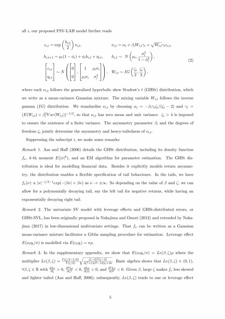
all i, our proposed FSV-LAH model further reads
zi,t = exp
(hi,t2
)νi,t, νi,t = αi + βiWi,tγi +
√Wi,tγiεi,t,
hi,t+1 = µi(1− φi) + φihi,t + ηi,t, hi,1 ∼ N
(µi,
σ2i
1− φ2i
),εi,t
ηi,t
∼ N0
0
, 1 ρiσi
ρiσi σ2i
, Wi,t ∼ IG
(ζi2,ζi2
),
(2)
where each νi,t follows the generalized hyperbolic skew Student’s t (GHSt) distribution, which
we write as a mean-variance Gaussian mixture. The mixing variable Wi,t follows the inverse
gamma (IG) distribution. We standardise νi,t by choosing αi = −βiγiζi/(ζi − 2) and γi =
(E(Wi,t) + β2i V ar(Wi,t))
−1/2, so that νi,t has zero mean and unit variance. ζi > 4 is imposed
to ensure the existence of a finite variance. The asymmetry parameter βi and the degrees of
freedom ζi jointly determine the asymmetry and heavy-tailedness of νi,t.
Suppressing the subscript i, we make some remarks:
Remark 1. Aas and Haff (2006) details the GHSt distribution, including its density function
fν , k-th moment E(|ν|k), and an EM algorithm for parameter estimation. The GHSt dis-
tribution is ideal for modelling financial data. Besides it explicitly models return asymme-
try, the distribution enables a flexible specification of tail behaviours. In the tails, we have
fν(ν) ∝ |ν|−ζ/2−1exp(−|βν| + βν) as ν → ±∞. So depending on the value of β and ζ, we can
allow for a polynomially decaying tail, say the left tail for negative returns, while having an
exponentially decaying right tail.
Remark 2. The univariate SV model with leverage effects and GHSt-distributed errors, or
GHSt-SVL, has been originally proposed in Nakajima and Omori (2012) and extended by Naka-
jima (2017) in low-dimensional multivariate settings. That fν can be written as a Gaussian
mean-variance mixture facilitates a Gibbs sampling procedure for estimation. Leverage effect
E(νtηt/σ) is modelled via E(εtηt) = σρ.
Remark 3. In the supplementary appendix, we show that E(νtηt/σ) = Le(β, ζ)ρ where the
multiplier Le(β, ζ) = Γ(ζ/2−1/2)Γ(ζ/2)
√(ζ−2)2(ζ−4)
2ζ2+(4β2−12)ζ+16. Basic algebra shows that Le(β, ζ) ∈ (0, 1),
∀β, ζ ∈ R with ∂Le∂ζ > 0, ∂
2Le∂ζ2 < 0, ∂Le∂|β| < 0, and ∂2Le
∂β2 < 0. Given β, large ζ makes fv less skewed
and lighter tailed (Aas and Haff, 2006); subsequently, Le(β, ζ) tends to one or leverage effect
5
tends to ρ. Given ζ > 4, the magnitude of leverage effect decreases to zero with |β| even though
ρ 6= 0. It means that if the return shock νt puts a large weight on the mixing variable Wt (i.e.
large |β|), leverage effect vanishes.
Due to the GHSt-SVL model used for both systematic and idiosyncratic components, our FSV-
LAH model makes possible the dependence structure along “stylised facts” including volatility
clustering, return asymmetry, leverage effects and heavy-tailedness. It is empirically important
to study the roles that they play in a high-dimensional setting, because a vast literature has
shown that such “stylised facts” are central to forecasting performance (see e.g., Nelson, 1991,
Yu, 2005 and Nakajima and Omori, 2012). Later in Section 3.1.3, we introduce Bayesian variable
selection to shrink ρi’s and βi’s so that we can also distinguish the systematic sources of leverage
effects and return asymmetry from idiosyncratic ones.
2.2 Identification of factors and loadings
To mitigate order dependence in the identification (of rotation, sign and scale) of factor models
(see e.g. Bai and Wang, 2015), we propose a pre-estimation step to pin down restrictions in Λ.
The first step relies on the principal component analysis (PCA) applied to yt which produces
ΛPCA. Rotation is identified by putting the i− 1 smallest loadings in absolute value in the i-th
column of ΛPCA to zero, i = 1, ..., n; and we fix the location of the zero loadings throughout.
The sign of the i-th factor and the i-column in Λ are identified by restricting the largest entry
in absolute value in the i-th column in ΛPCA to be positive; this is to say Λkii > 0, where
ki = arg maxk|ΛPCAki |; k = 1, ..., n
and Xij denotes the i, j-th element of matrix X. The scale
is identified by restricting µi = 0 for i = 1, .., n.
With ki = i and without the PCA step, the identification scheme is identical to the one in
Kastner et al. (2017) who argue that this scheme does not impose the disproportionate effect of
the n leading variables on factor dynamics. We choose the zero restrictions on Λ using the extra
PCA step, because PCs are order-invariant. As a result, the identified factor space is close to
the one spanned by the unique order-invariant PCs.
6
3 Bayesian estimation
This section introduces our proposed Bayesian estimation procedure for the FSV-LAH model.
Conditional on Λ and system parameters, ft and ut can be sampled directly. This gives n +
N univariate GHSt-SVL models, which can be analysed in parallel in each MCMC run on a
computer with multi-threading CPUs. We first provide a sampling algorithm to this univariate
problem that is more efficient but slightly more computationally intensive than the one used in
Nakajima and Omori (2012) and Nakajima (2017) and second a sampling procedure for drawing
Λ from its full conditional posterior distribution when N or/and n become large.
3.1 Efficient estimation of the GHSt-SVL model
In each run of the full MCMC sampler, we obtain a sample of zt = (f ′t , u′t)′ ∈ Rn+N conditional
on Λ with each zi,t seen as a separate GHSt-SVL model. Suppressing the subscript i in Section
3.1.1 and 3.1.2 and letting θ = (σ, ρ, φ, µ, β, ζ) collect the model parameters and x1:t denote
x1, x2, ..., xt, we propose a Gibbs sampler for zt that iterates over
1. Sampling (h1:T ,W1:T )|z1:T , θ;
2. Sampling θ|z1:T , h1:T ,W1:T .
The key feature here is the joint sampling of the entire trajectories h1:T and W1:T as a single
block via an efficient particle Gibbs algorithm. In comparison, Nakajima and Omori (2012)
sample ht|Wt using a multi-move sampler (Shephard and Pitt, 1997), and subsequently sample
Wt|ht using a Metropolis-Hastings (MH) step.Our procedure avoids the autocorrelation cause
by the iterative sampling between ht|Wt and Wt|ht.
3.1.1 Particle Gibbs with ancestor sampling for sampling (h1:T ,W1:T )|z1:T , θ
Let xt denote (ht,Wt)′ and θ be suppressed. To sample from p(x1:T |z1:T ), we modify the particle
Gibbs with ancestor sampling (PGAS) method developed by Lindsten et al. (2014). Compared
with the usual forward-filtering and backward-smoothing with importance sampling (see Shep-
hard and Pitt, 1997 and Watanabe and Omori, 2004), particle Gibbs (PG, see e.g., Doucet
et al., 2001 and Chopin et al., 2013) can be computationally advantageous if a small number of
particles is used in the one-way simulation from t = 1 to T with sequential Monte Carlo.
7
Although the basic PG with input xold1:T (the old draw in the Markov chain) and output xnew1:T
(the new draw) is straightforward to implement, it suffers from the well-documented problem of
particle degeneration (see e.g., Pitt and Shephard, 1999b and Snyder et al., 2008)— p(xnew1:T =
xold1:T ) is bounded away from zero, which leads to poor mixing. According to Lindsten et al.
(2014), PGAS circumvents the global degeneration problem by cutting xold1:T into pieces of xt1:t2
where t1 < t2 and t1, t2 = 1, ..., T . Consequently, xnew1:T 6= xold1:T a.s. Lindsten et al. (2014) show
that PGAS improves the mixing of latent processes in a standard SV model.
We briefly discuss the adoption of PGAS in the GHSt-SVL model with details left in the
supplementary appendix. Suppose at t − 1, we have a particle system containing M par-
ticles xi1:t−1Mi=1 and associated weights ωit−1Mi=1 which approximates the filtering density
p(x1:t−1|z1:t−1) by p(x1:t−1|z1:t−1) ∝∑M
i=1 ωit−1D(x1:t−1 − xi1:t−1), where D(.) is the Dirac delta
function. PGAS propagates the particle system by first sampling ait, xtMi=1 from
It(at, xt) ∝ ωatt−1p(xt|xatt−1, zt−1), (3)
where p(xt|xt−1, zt−1) is the transition density of (ht,Wt)′, i.e.
p(xt|xt−1, zt−1) ∝ exp
(µ(1− φ) + φht−1 + ρσεt−1
(1− ρ2)σ2ht −
h2t
12(1− ρ2)σ2
)·W−
ζ2−1
t exp
(−ζ
2W−1t
)
with εt−1 = (zt−1e−ht−1/2−α−βWt−1γ)/
√Wt−1γ accounting for the leverage effect (Yu, 2005);
and where at indexes the ancestor particle, i.e. xi1:t = (xait1:t−1, x
it). Second, we augment the parti-
cle system with xold1:T by assigning xM+1t = xoldt and sample the ancestor according to P(aM+1
t =
i) ∝ ωit−1p(x?t |xit−1, zt−1), which rewrites the history of xold1:t by xM+1
1:t = (xaM+1t
1:t−1 , xM+1t ). The
augmented system at each t is then re-weighted according to
ωit ∝ p(zt|xit), for i = 1, ...,M + 1. (4)
Once the propagation reaches t = T , PGAS samples a new path xnew1:T from p(x1:T |z1:T ) ∝
ωiTD(x1:T − xi1:T ).
When propagating the particle system, PGAS breaks the dependence of xnew1:T on xold1:T , i.e.
the ancestral dependence, which allows for a much smaller number of particles than PG while
8
remaining functionality. It is however important to notice that PGAS does not break the depen-
dence between xnewt1:t2 on xoldt1:t2 for some t1 and t2 (ancestor sampling does not solve local particle
degeneration). We propose an efficient importance sampling procedure in the next section that
ensures local efficiency and uses a small number of particles. This helps reduce computational
burden from fewer function evaluations and Monte Carlo noise that is non-negligible in high-
dimensional models (Dang et al., 2015).
3.1.2 Approximating p(h1:T ,W1:T |z1:T , θ) via efficient importance sampling
Drawing xt from the transition density p(xt|xt−1, zt−1) renders the effective sample size small and
thus requires a large number of particles (in PG particularly) and constant resampling to avoid
particle degeneration at a cost of efficiency. The remedy is to incorporate an importance sampling
(IS) step that uses a proposal density q(xt|xt−1, zt−1,F), where F is a chosen information set,
to generate “informative” draws.
To maximise efficiency while utilising the small number of particles allowed in PGAS, we
propose to choose F = z1:T for the GHSt-SVL model. This is motivated by the fact that we
can express the likelihood of the GHSt-SVL model as
L(z1:T ) =
∫p(z1:T |x1:T )p(x1:T )
q(x1:T |z1:T )q(x1:T |z1:T )dx1:T
=
∫p(z1|x1)p(x1)
q(x1|z1:T )
T∏t=2
p(zt|xt)p(xt|xt−1, zt−1)
q(xt|xt−1, z1:T )q(x1:T |z1:T )dx1:T ,
(5)
where p(zt|xt) is Gaussian with mean eht/2(α + βWtγ) and variance γ2Wteht ; and q(x1:T |z1:T )
is a global approximating density that can be factorised into terms such as q(xt|xt−1, z1:T ). It is
evident that choosing F = z1:T has an informational advantage over other choices such as the
one in Pitt and Shephard (1999b) with F = zt, zt+1. Draws from q(xt|xt−1, z1:T ) are the best
“guesses” as they are informed by the full data information. Consequently, the effective sample
size is large even when the number of particle is small. Scharth and Kohn (2016) show that
the (frequentist) efficient importance sampling (EIS) method of Richard and Zhang (2007) and
Jung and Liesenfeld (2001) can be used in a particle marginal Metropolis Hastings (PMMH)
algorithm (Andrieu et al., 2010) for SV models to marginalise the log variance process and
accurately estimate the likelihood using as few as two particles.
9
It is worthwhile noticing that p(z1:T |x1:T )p(x1:T ) contains the product of Gaussian and IG
densities, which are exponential family distributions that are closed under multiplication. We
use this conjugacy property and choose q(x1:T |z1:T ) to be also a product of Gaussians and IG’s
so that q(x1:T |z1:T ) well approximates p(z1:T |x1:T )p(x1:T ). Because the integrand in (5) can be
factorised, we choose
q(xt|xt−1, z1:T ) ∝ exp
(btht −
1
2cth
2t
)·W st
t exp(rtW
−1t
). (6)
Let δt = (bt, ct, st, rt)′ collect the proposal density parameters which are functions of z1:T . In
the supplementary appendix, we show that given δt the candidate draws of ht and Wt can be
generated from N(µht , vht) with vht = [(1− ρ2)σ2]/[1 + (1− ρ2)σ2ct] and µht = vtbt + vt[µ(1−
φ) + φht−1 + ρσεt−1]/[(1− ρ2)σ2] and IG(st + ζ/2, rt + ζ/2), respectively. To determine δt, we
minimise the squared distance between log[p(zt|xt)p(xt|xt−1, zt−1)] and log q(xt|xt−1, z1:T ). The
latter being linear in δt conveniently allows us to write the minimisation problem as an OLS
with solution δt (ignoring constant) given by (X ′X )−1X ′Y. For j = 1, ..., J , X is J-by-5 with
the j-th row(
1, h(j)t ,−(h
(j)t )2/2, logW
(j)t , 1/W
(j)t
)and Y is J-by-1 with the j-th element
−
(zt − exp
(h
(j)t /2
)(α+ βW
(j)t γ
))2
2γ2W(j)t exp
(h
(j)t
) − g(δt+1, zt−1, h
(j)t , h
(j)t−1,W
(j)t ,W
(j)t−1
),
where h(j)t and W
(j)t are the j-th draw from N(µoldht , v
oldht
) and IG(soldt + ζ/2, roldt + ζ/2), respec-
tively, with the proposal density parameters δoldt obtained in the previous run of the Markov
chain.
Importantly, g(δt+1, zt−1, h
(j)t , h
(j)t−1,W
(j)t ,W
(j)t−1
)is a function (see supplementary appendix)
that depends on δt+1, which unfortunately creates computational overhead cost because δt+1
has to be determined prior to δt, resulting in an un-parallelisable backward recursion (see also
Richard and Zhang, 2007). This backward-shift of δt+1, a function of z1:T , is however crucial for
obtaining an efficient proposal density that enables us to generate draws of xt using information
in z1:T . In simulation studies and empirical studies, we choose J to be 50 to keep the computa-
tional cost of computing X ′X to the minimum. Lastly, with q(xt|xt−1, z1:T ) determined, PGAS
10
with EIS, or PGAS-EIS, changes step (3) and step (4) into
It(at, xt) ∝ ωatt−1q(xt|xatt−1, z1:T ), and ωit ∝
p(zt|xit)p(xit|xit−1, zt−1)
q(xit|xit−1, z1:T ).
Analysing the optimal number of particles M is beyond the scope of this research. Neverthe-
less, we use the criterion in Scharth and Kohn (2016) who apply EIS to estimate a standard SV
model via PMMH: M is such that the IS estimate of the variance of logL(z1:T ) equals approxi-
mately one; see also Pitt et al. (2012). In our simulation studies (except for one extreme case)
and empirical applications, M varies around 10. So we choose M = 20 to be conservative, a
very small number compared to other studies using particle methods.
3.1.3 Sampling θ|z1:T , h1:T ,W1:T and variable selection in the FSV-LAH model
Given hi,1:T , Wi,1:T , and zi,1:T , we can sample θi series-by-series. We here focus on σi, ρi and
βi, and sample the remaining parameters according to Nakajima and Omori (2012). We shrink
some ρi’s and βi’s to zero via Bayesian variable selection which avoids 22(n+N) model comparisons
and keeps the model parsimonious in a data-driven way. Non-zero ρi’s and βi’s also address the
systematic and idiosyncratic sources of leverage effects and return asymmetry.
Let p0(·) and p(|·) denote prior and conditional posterior distribution, respectively. For the
i-th series, the joint posterior distribution p(σi, ρi|·) is
p(σi, ρi|·) ∝ p0(σi, ρi)σ−Ti (1− ρ2
i )−T−1
2 exp
−
(1− φ2i )h
2i,1
2σ2i
−T−1∑t=1
(hi,t+1 − φhi,t − ρiσiεi,t)2
2σ2i (1− ρ2
i )
,
where hi,t = hi,t − µi. Re-parametrising ϑi = ρiσi and $i = σ2i (1 − ρ2
i ) as in Jacquier et al.
(2004) to facilitate the shrinkage prior and posterior used in Bayesian variable selection, we
introduce an axillary variable ∆ and define the joint prior as p0(ϑi|$i,∆)p0($i)p0(∆) where
p0($i) = IG(s0, r0) and
p0(ϑi|$i,∆) = ∆D(ϑi) + (1−∆)N(ϑ0, v2ϑ$i).
Here ∆ with p0(∆) = Beta(ς1, ς2) indicates non-zero probability at ϑi = 0 (Clyde and George,
2004), i.e. no leverage effect. For i = 1, ..., n+N , new $i is generated from p($i|·) = IG(s0 +
11
T/2, r0 + ri/2) with ri =∑T−1
t=1 (hi,t+1 − φhi,t)2 − µ2ϑi/σ2
ϑi+ ϑ2
0/v2ϑ and ϑi from
p(ϑi|·) =(1−∆i)D(ϑi)
∆iσ2ϑi
+ 1−∆i+
∆iσ2ϑi
σ2ϑi
+ 1−∆iN(µϑi , σ
2ϑi$i), (7)
with σ2ϑi
= σϑi exp(µϑ2i/2σ2
ϑi$i) and ∆i drawn from p(∆i|·) = Beta(ς1 +
∑n+Ni=1 1(ς2+6=0), ς2 +
n+N −∑n+N
i=1 1(ϑi 6=0)), where 1(.) denotes the indicator function, and with posterior variance
and mean given by
σ2ϑi
=
1
v2ϑ
+
T−1∑t=1
ε2i,t
−1
, µϑ = σ2ϑi
ϑ0
v2ϑ
+
T−1∑t=1
εi,t(hi,t+1 − φhi,t)
.
The Markov chain is updated by σi =√ϑ2i +$i and ρi = ϑi/σi.
It is standard to show that with a normal prior, the asymmetry parameter βi has a normal
posterior. So we can modify the prior same as the above and obtain a shrinkage posterior in the
form of (7). The supplementary appendix details how to sample the remaining parameters.
3.2 Sampling factors and factor loadings
Define yi,t = yi,t−(αn+i+βn+iWn+iγn+i)ehn+i,t/2 for i = 1, ..., N and Fi,t = (αi+βiWi,tγi)e
hi,t/2
for i = 1, ..., n. Conditional on log variances h1:T = h1,1:T , ..., hn+N,1:T and mixing components
W1:T = W1,1:T , ...,Wn+N,1:T , we have yt|ft ∼ N(Λft, Ut) and ft ∼ N(Ft, Vt), where yt =
(y1,t, ..., yN,t)′, Ft = (F1,t, ..., Fn,t)
′, Ut = diag(Wn+1,tγ2n+1e
hn+1,t , ...,Wn+N,tγ2n+Ne
hn+N,t), and
Vt = diag(W1,tγ21eh1,t , ...,Wn,tγ
2nehn,t). So we can draw ft from N(µft ,Σft) with
Σft = (Λ′U−1t Λ + V −1
t ), µft = Σft(Λ′U−1t yt + V −1
t Ft).
We assume an independent normal prior p0(Λij) = N(Λ0, v2Λ) for all free elements in Λ.
Because Λ and ft show up in the likelihood in product form, efficient sampling usually replies on
a Rao-Blackwellisation (RB) procedure to marginalise ft and sample Λ using a MH algorithm
(Chib et al., 2006) based on p(Λ|·) ∝ p(y1:T |Λ)p0(Λ). Notice that the conditional posterior is
given by
p(y1:T |Λ) ∝ exp
(−1
2
T∑t=1
log |Ωt|+ (yt − ΛFt)′Ω−1t (yt − ΛFt)
), (8)
12
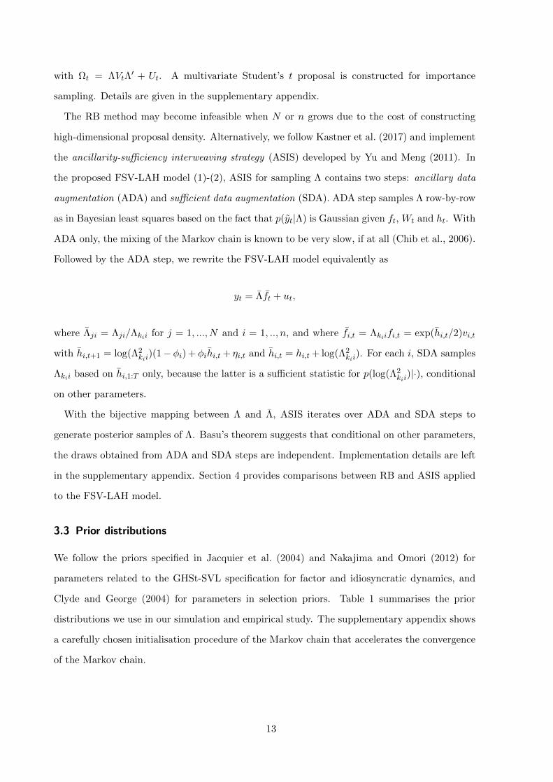
with Ωt = ΛVtΛ′ + Ut. A multivariate Student’s t proposal is constructed for importance
sampling. Details are given in the supplementary appendix.
The RB method may become infeasible when N or n grows due to the cost of constructing
high-dimensional proposal density. Alternatively, we follow Kastner et al. (2017) and implement
the ancillarity-sufficiency interweaving strategy (ASIS) developed by Yu and Meng (2011). In
the proposed FSV-LAH model (1)-(2), ASIS for sampling Λ contains two steps: ancillary data
augmentation (ADA) and sufficient data augmentation (SDA). ADA step samples Λ row-by-row
as in Bayesian least squares based on the fact that p(yt|Λ) is Gaussian given ft, Wt and ht. With
ADA only, the mixing of the Markov chain is known to be very slow, if at all (Chib et al., 2006).
Followed by the ADA step, we rewrite the FSV-LAH model equivalently as
yt = Λft + ut,
where Λji = Λji/Λkii for j = 1, ..., N and i = 1, .., n, and where fi,t = Λkiifi,t = exp(hi,t/2)vi,t
with hi,t+1 = log(Λ2kii
)(1− φi) + φihi,t + ηi,t and hi,t = hi,t + log(Λ2kii
). For each i, SDA samples
Λkii based on hi,1:T only, because the latter is a sufficient statistic for p(log(Λ2kii
)|·), conditional
on other parameters.
With the bijective mapping between Λ and Λ, ASIS iterates over ADA and SDA steps to
generate posterior samples of Λ. Basu’s theorem suggests that conditional on other parameters,
the draws obtained from ADA and SDA steps are independent. Implementation details are left
in the supplementary appendix. Section 4 provides comparisons between RB and ASIS applied
to the FSV-LAH model.
3.3 Prior distributions
We follow the priors specified in Jacquier et al. (2004) and Nakajima and Omori (2012) for
parameters related to the GHSt-SVL specification for factor and idiosyncratic dynamics, and
Clyde and George (2004) for parameters in selection priors. Table 1 summarises the prior
distributions we use in our simulation and empirical study. The supplementary appendix shows
a carefully chosen initialisation procedure of the Markov chain that accelerates the convergence
of the Markov chain.
13
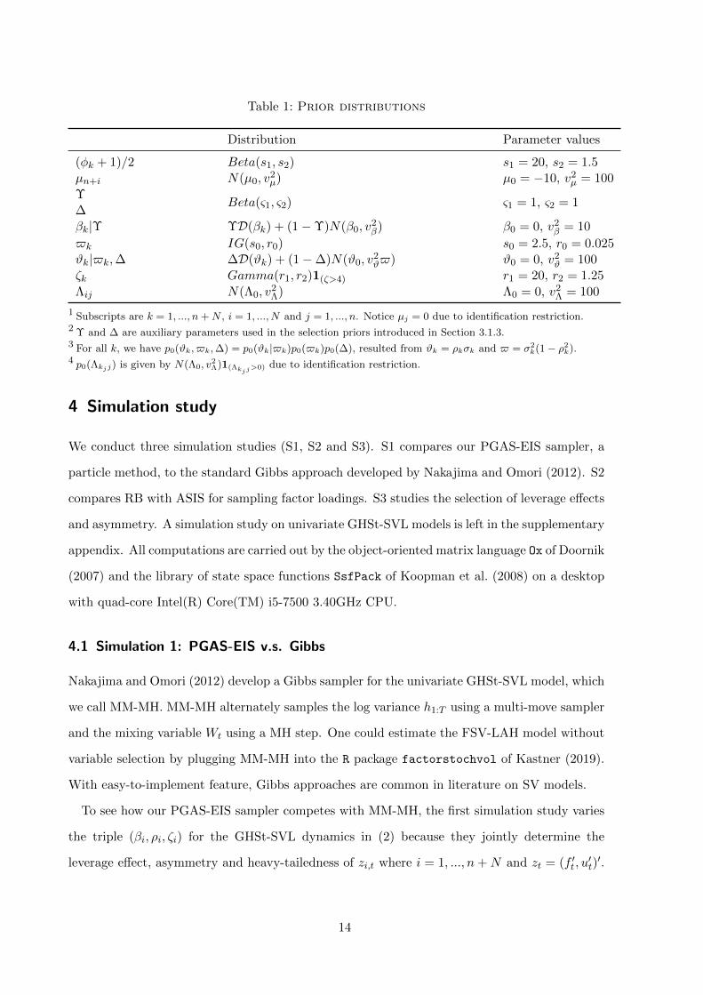
Table 1: Prior distributions
Distribution Parameter values
(φk + 1)/2 Beta(s1, s2) s1 = 20, s2 = 1.5µn+i N(µ0, v
2µ) µ0 = −10, v2
µ = 100
ΥBeta(ς1, ς2) ς1 = 1, ς2 = 1
∆βk|Υ ΥD(βk) + (1−Υ)N(β0, v
2β) β0 = 0, v2
β = 10
$k IG(s0, r0) s0 = 2.5, r0 = 0.025ϑk|$k,∆ ∆D(ϑk) + (1−∆)N(ϑ0, v
2ϑ$) ϑ0 = 0, v2
ϑ = 100ζk Gamma(r1, r2)1(ζ>4) r1 = 20, r2 = 1.25
Λij N(Λ0, v2Λ) Λ0 = 0, v2
Λ = 100
1 Subscripts are k = 1, ..., n+N , i = 1, ..., N and j = 1, ..., n. Notice µj = 0 due to identification restriction.2 Υ and ∆ are auxiliary parameters used in the selection priors introduced in Section 3.1.3.3 For all k, we have p0(ϑk, $k,∆) = p0(ϑk|$k)p0($k)p0(∆), resulted from ϑk = ρkσk and $ = σ2
k(1− ρ2k).
4 p0(Λkjj) is given by N(Λ0, v2Λ)1(Λkjj
>0) due to identification restriction.
4 Simulation study
We conduct three simulation studies (S1, S2 and S3). S1 compares our PGAS-EIS sampler, a
particle method, to the standard Gibbs approach developed by Nakajima and Omori (2012). S2
compares RB with ASIS for sampling factor loadings. S3 studies the selection of leverage effects
and asymmetry. A simulation study on univariate GHSt-SVL models is left in the supplementary
appendix. All computations are carried out by the object-oriented matrix language Ox of Doornik
(2007) and the library of state space functions SsfPack of Koopman et al. (2008) on a desktop
with quad-core Intel(R) Core(TM) i5-7500 3.40GHz CPU.
4.1 Simulation 1: PGAS-EIS v.s. Gibbs
Nakajima and Omori (2012) develop a Gibbs sampler for the univariate GHSt-SVL model, which
we call MM-MH. MM-MH alternately samples the log variance h1:T using a multi-move sampler
and the mixing variable Wt using a MH step. One could estimate the FSV-LAH model without
variable selection by plugging MM-MH into the R package factorstochvol of Kastner (2019).
With easy-to-implement feature, Gibbs approaches are common in literature on SV models.
To see how our PGAS-EIS sampler competes with MM-MH, the first simulation study varies
the triple (βi, ρi, ζi) for the GHSt-SVL dynamics in (2) because they jointly determine the
leverage effect, asymmetry and heavy-tailedness of zi,t where i = 1, ..., n+N and zt = (f ′t , u′t)′.
14
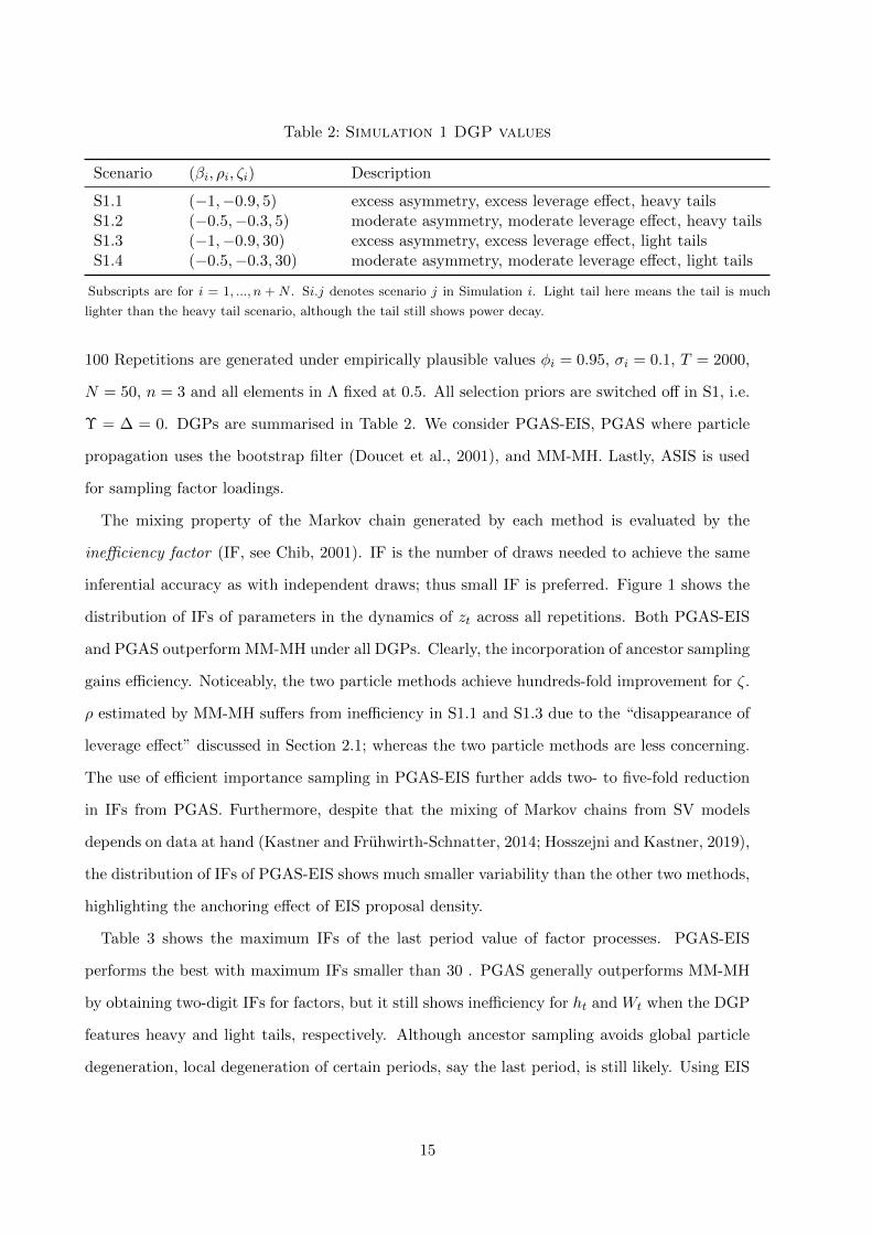
Table 2: Simulation 1 DGP values
Scenario (βi, ρi, ζi) Description
S1.1 (−1,−0.9, 5) excess asymmetry, excess leverage effect, heavy tailsS1.2 (−0.5,−0.3, 5) moderate asymmetry, moderate leverage effect, heavy tailsS1.3 (−1,−0.9, 30) excess asymmetry, excess leverage effect, light tailsS1.4 (−0.5,−0.3, 30) moderate asymmetry, moderate leverage effect, light tails
Subscripts are for i = 1, ..., n + N . Si.j denotes scenario j in Simulation i. Light tail here means the tail is much
lighter than the heavy tail scenario, although the tail still shows power decay.
100 Repetitions are generated under empirically plausible values φi = 0.95, σi = 0.1, T = 2000,
N = 50, n = 3 and all elements in Λ fixed at 0.5. All selection priors are switched off in S1, i.e.
Υ = ∆ = 0. DGPs are summarised in Table 2. We consider PGAS-EIS, PGAS where particle
propagation uses the bootstrap filter (Doucet et al., 2001), and MM-MH. Lastly, ASIS is used
for sampling factor loadings.
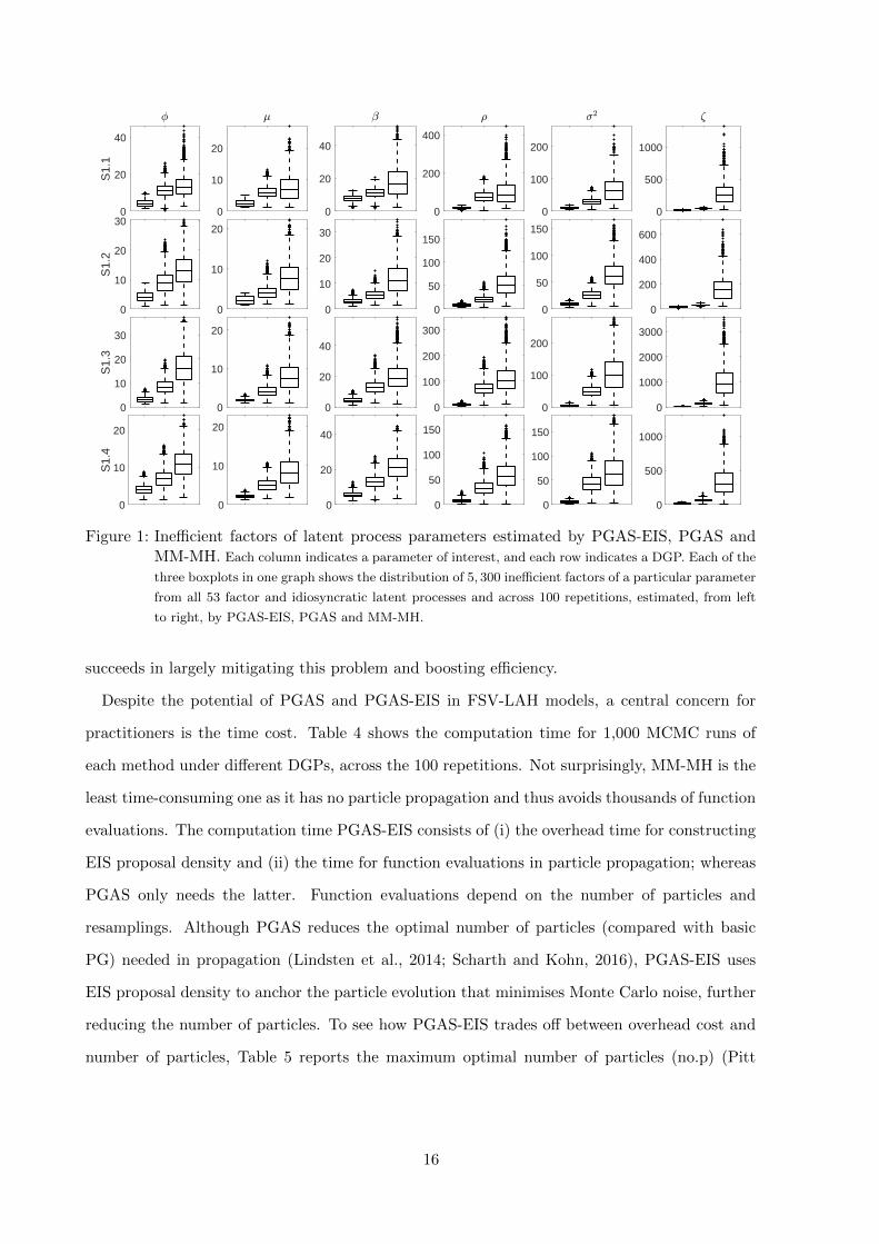
The mixing property of the Markov chain generated by each method is evaluated by the
inefficiency factor (IF, see Chib, 2001). IF is the number of draws needed to achieve the same
inferential accuracy as with independent draws; thus small IF is preferred. Figure 1 shows the
distribution of IFs of parameters in the dynamics of zt across all repetitions. Both PGAS-EIS
and PGAS outperform MM-MH under all DGPs. Clearly, the incorporation of ancestor sampling
gains efficiency. Noticeably, the two particle methods achieve hundreds-fold improvement for ζ.
ρ estimated by MM-MH suffers from inefficiency in S1.1 and S1.3 due to the “disappearance of
leverage effect” discussed in Section 2.1; whereas the two particle methods are less concerning.
The use of efficient importance sampling in PGAS-EIS further adds two- to five-fold reduction
in IFs from PGAS. Furthermore, despite that the mixing of Markov chains from SV models
depends on data at hand (Kastner and Fruhwirth-Schnatter, 2014; Hosszejni and Kastner, 2019),
the distribution of IFs of PGAS-EIS shows much smaller variability than the other two methods,
highlighting the anchoring effect of EIS proposal density.
Table 3 shows the maximum IFs of the last period value of factor processes. PGAS-EIS
performs the best with maximum IFs smaller than 30 . PGAS generally outperforms MM-MH
by obtaining two-digit IFs for factors, but it still shows inefficiency for ht and Wt when the DGP
features heavy and light tails, respectively. Although ancestor sampling avoids global particle
degeneration, local degeneration of certain periods, say the last period, is still likely. Using EIS
15
0
20
40
S1.
1
0
10
20
0
20
40
0
200
400
0
100
200
0
500
1000
0
10
20
30
S1.
2
0
10
20
0
10
20
30
0
50
100
150
0
50
100
150
0
200
400
600
0
10
20
30
S1.
3
0
10
20
0
20
40
0
100
200
300
0
100
200
0
1000
2000
3000
0
10
20
S1.
4
0
10
20
0
20
40
0
50
100
150
0
50
100
150
0
500
1000
Figure 1: Inefficient factors of latent process parameters estimated by PGAS-EIS, PGAS andMM-MH. Each column indicates a parameter of interest, and each row indicates a DGP. Each of the
three boxplots in one graph shows the distribution of 5, 300 inefficient factors of a particular parameter
from all 53 factor and idiosyncratic latent processes and across 100 repetitions, estimated, from left
to right, by PGAS-EIS, PGAS and MM-MH.
succeeds in largely mitigating this problem and boosting efficiency.
Despite the potential of PGAS and PGAS-EIS in FSV-LAH models, a central concern for
practitioners is the time cost. Table 4 shows the computation time for 1,000 MCMC runs of
each method under different DGPs, across the 100 repetitions. Not surprisingly, MM-MH is the
least time-consuming one as it has no particle propagation and thus avoids thousands of function
evaluations. The computation time PGAS-EIS consists of (i) the overhead time for constructing
EIS proposal density and (ii) the time for function evaluations in particle propagation; whereas
PGAS only needs the latter. Function evaluations depend on the number of particles and
resamplings. Although PGAS reduces the optimal number of particles (compared with basic
PG) needed in propagation (Lindsten et al., 2014; Scharth and Kohn, 2016), PGAS-EIS uses
EIS proposal density to anchor the particle evolution that minimises Monte Carlo noise, further
reducing the number of particles. To see how PGAS-EIS trades off between overhead cost and
number of particles, Table 5 reports the maximum optimal number of particles (no.p) (Pitt
16
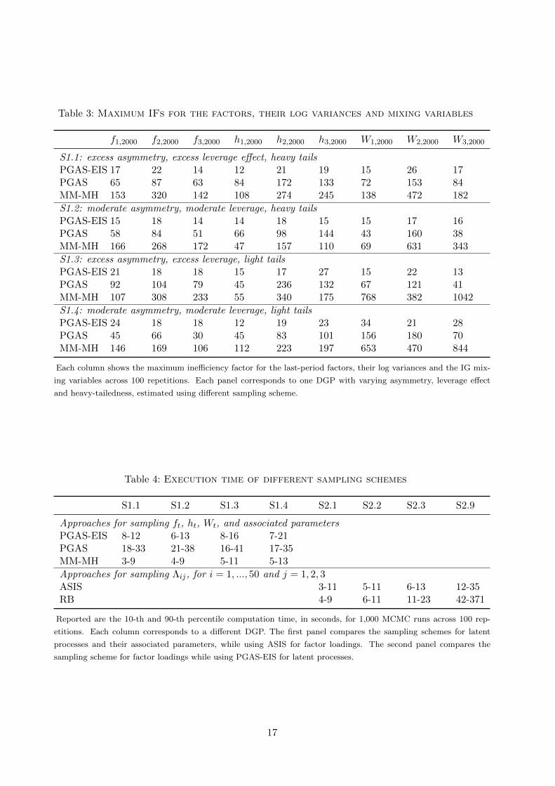
Table 3: Maximum IFs for the factors, their log variances and mixing variables
f1,2000 f2,2000 f3,2000 h1,2000 h2,2000 h3,2000 W1,2000 W2,2000 W3,2000
S1.1: excess asymmetry, excess leverage effect, heavy tailsPGAS-EIS 17 22 14 12 21 19 15 26 17PGAS 65 87 63 84 172 133 72 153 84MM-MH 153 320 142 108 274 245 138 472 182
S1.2: moderate asymmetry, moderate leverage, heavy tailsPGAS-EIS 15 18 14 14 18 15 15 17 16PGAS 58 84 51 66 98 144 43 160 38MM-MH 166 268 172 47 157 110 69 631 343
S1.3: excess asymmetry, excess leverage, light tailsPGAS-EIS 21 18 18 15 17 27 15 22 13PGAS 92 104 79 45 236 132 67 121 41MM-MH 107 308 233 55 340 175 768 382 1042
S1.4: moderate asymmetry, moderate leverage, light tailsPGAS-EIS 24 18 18 12 19 23 34 21 28PGAS 45 66 30 45 83 101 156 180 70MM-MH 146 169 106 112 223 197 653 470 844
Each column shows the maximum inefficiency factor for the last-period factors, their log variances and the IG mix-
ing variables across 100 repetitions. Each panel corresponds to one DGP with varying asymmetry, leverage effect
and heavy-tailedness, estimated using different sampling scheme.
Table 4: Execution time of different sampling schemes
S1.1 S1.2 S1.3 S1.4 S2.1 S2.2 S2.3 S2.9
Approaches for sampling ft, ht, Wt, and associated parametersPGAS-EIS 8-12 6-13 8-16 7-21PGAS 18-33 21-38 16-41 17-35MM-MH 3-9 4-9 5-11 5-13
Approaches for sampling Λij, for i = 1, ..., 50 and j = 1, 2, 3ASIS 3-11 5-11 6-13 12-35RB 4-9 6-11 11-23 42-371
Reported are the 10-th and 90-th percentile computation time, in seconds, for 1,000 MCMC runs across 100 rep-
etitions. Each column corresponds to a different DGP. The first panel compares the sampling schemes for latent
processes and their associated parameters, while using ASIS for factor loadings. The second panel compares the
sampling scheme for factor loadings while using PGAS-EIS for latent processes.
17
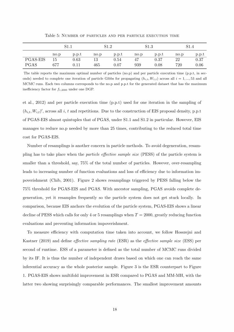
Table 5: Number of particles and per particle execution time
S1.1 S1.2 S1.3 S1.4
no.p p.p.t no.p p.p.t no.p p.p.t no.p p.p.t
PGAS-EIS 15 0.63 13 0.54 47 0.37 22 0.37PGAS 677 0.11 465 0.07 939 0.08 720 0.06
The table reports the maximum optimal number of particles (no.p) and per particle execution time (p.p.t, in sec-
onds) needed to complete one iteration of particle Gibbs for propagating (hi,t,W1,t) across all i = 1, ..., 53 and all
MCMC runs. Each two columns corresponds to the no.p and p.p.t for the generated dataset that has the maximum
inefficiency factor for f1,2000 under one DGP.
et al., 2012) and per particle execution time (p.p.t) used for one iteration in the sampling of
(hi,t,Wi,t)′, across all i, t and repetitions. Due to the construction of EIS proposal density, p.p.t
of PGAS-EIS almost quintuples that of PGAS, under S1.1 and S1.2 in particular. However, EIS
manages to reduce no.p needed by more than 25 times, contributing to the reduced total time
cost for PGAS-EIS.
Number of resamplings is another concern in particle methods. To avoid degeneration, resam-
pling has to take place when the particle effective sample size (PESS) of the particle system is
smaller than a threshold, say, 75% of the total number of particles. However, over-resampling
leads to increasing number of function evaluations and loss of efficiency due to information im-
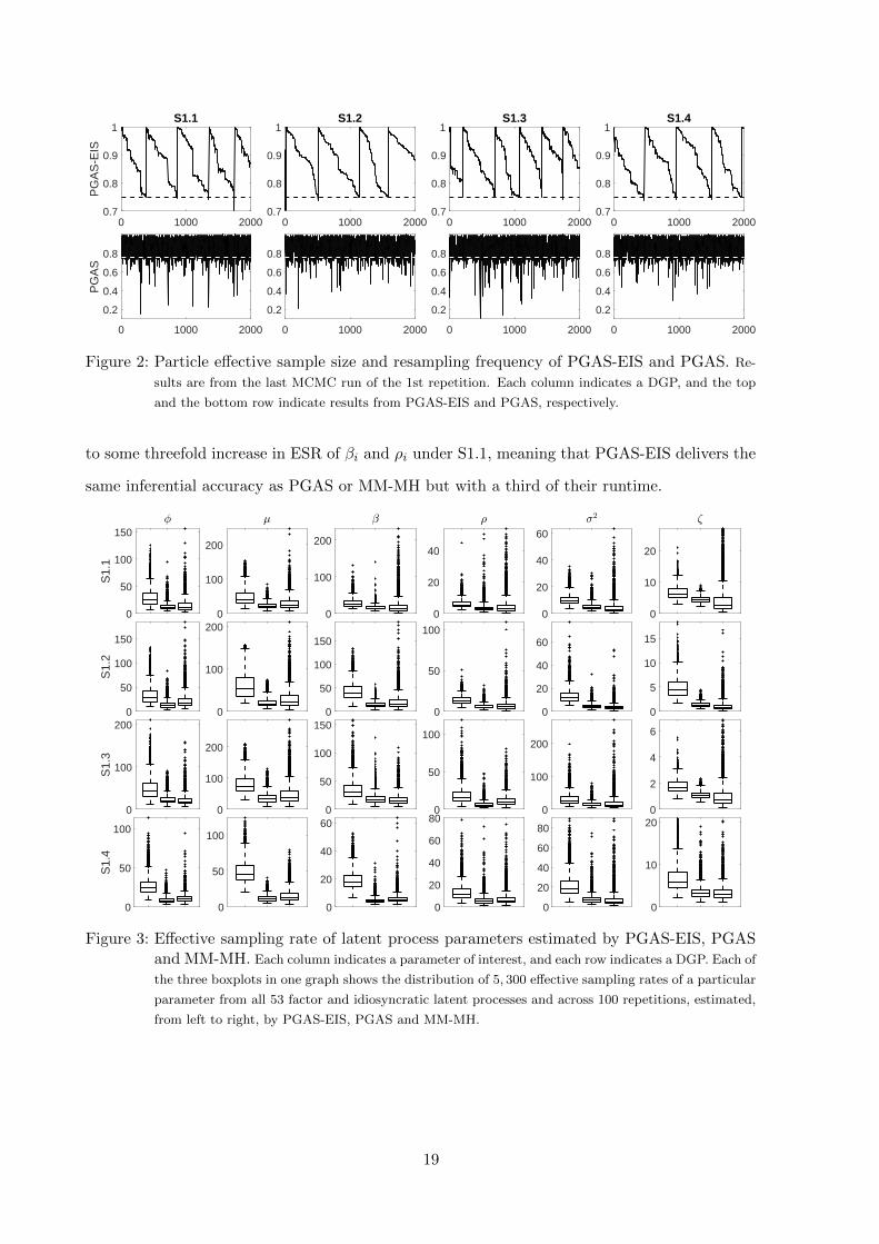
poverishment (Chib, 2001). Figure 2 shows resamplings triggered by PESS falling below the
75% threshold for PGAS-EIS and PGAS. With ancestor sampling, PGAS avoids complete de-
generation, yet it resamples frequently so the particle system does not get stuck locally. In
comparison, because EIS anchors the evolution of the particle system, PGAS-EIS shows a linear
decline of PESS which calls for only 4 or 5 resamplings when T = 2000, greatly reducing function
evaluations and preventing information impoverishment.
To measure efficiency with computation time taken into account, we follow Hosszejni and
Kastner (2019) and define effective sampling rate (ESR) as the effective sample size (ESS) per
second of runtime. ESS of a parameter is defined as the total number of MCMC runs divided
by its IF. It is thus the number of independent draws based on which one can reach the same
inferential accuracy as the whole posterior sample. Figure 3 is the ESR counterpart to Figure
1. PGAS-EIS shows multifold improvement in ESR compared to PGAS and MM-MH, with the
latter two showing surprisingly comparable performances. The smallest improvement amounts
18
0 1000 20000.7
0.8
0.9
1S1.3
0 1000 2000
0.2
0.4
0.6
0.8
0 1000 20000.7
0.8
0.9
1
PG
AS
-EIS
S1.1
0 1000 2000
0.2
0.4
0.6
0.8
PG
AS
0 1000 20000.7
0.8
0.9
1S1.4
0 1000 2000
0.2
0.4
0.6
0.8
0 1000 20000.7
0.8
0.9
1S1.2
0 1000 2000
0.2
0.4
0.6
0.8
Figure 2: Particle effective sample size and resampling frequency of PGAS-EIS and PGAS. Re-
sults are from the last MCMC run of the 1st repetition. Each column indicates a DGP, and the top
and the bottom row indicate results from PGAS-EIS and PGAS, respectively.
to some threefold increase in ESR of βi and ρi under S1.1, meaning that PGAS-EIS delivers the
same inferential accuracy as PGAS or MM-MH but with a third of their runtime.
0
50
100
150
S1.
1
0
100
200
0
100
200
0
20
40
0
20
40
60
0
10
20
0
50
100
150
S1.
2
0
100
200
0
50
100
150
0
50
100
0
20
40
60
0
2
4
6
0
100
200
S1.
3
0
100
200
0
50
100
150
0
50
100
0
100
200
0
5
10
15
0
50
100
S1.
4
0
50
100
0
20
40
60
0
20
40
60
80
0
20
40
60
80
0
10
20
Figure 3: Effective sampling rate of latent process parameters estimated by PGAS-EIS, PGASand MM-MH. Each column indicates a parameter of interest, and each row indicates a DGP. Each of
the three boxplots in one graph shows the distribution of 5, 300 effective sampling rates of a particular
parameter from all 53 factor and idiosyncratic latent processes and across 100 repetitions, estimated,
from left to right, by PGAS-EIS, PGAS and MM-MH.
19
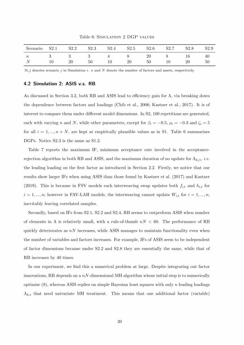
Table 6: Simulation 2 DGP values
Scenario S2.1 S2.2 S2.3 S2.4 S2.5 S2.6 S2.7 S2.8 S2.9
n 3 3 3 4 8 20 8 16 40N 10 20 50 10 20 50 10 20 50
Si.j denotes scenario j in Simulation i. n and N denote the number of factors and assets, respectively.
4.2 Simulation 2: ASIS v.s. RB
As discussed in Section 3.2, both RB and ASIS lead to efficiency gain for Λ, via breaking down
the dependence between factors and loadings (Chib et al., 2006; Kastner et al., 2017). It is of
interest to compare them under different model dimensions. In S2, 100 repetitions are generated,
each with varying n and N , while other parameters, except for βi = −0.5, ρi = −0.3 and ζi = 5
for all i = 1, ..., n + N , are kept at empirically plausible values as in S1. Table 6 summarises
DGPs. Notice S2.3 is the same as S1.2.
Table 7 reports the maximum IF, minimum acceptance rate involved in the acceptance-
rejection algorithm in both RB and ASIS, and the maximum duration of no update for Λk11, i.e.
the leading loading on the first factor as introduced in Section 2.2. Firstly, we notice that our
results show larger IFs when using ASIS than those found by Kastner et al. (2017) and Kastner
(2019). This is because in FSV models each interweaving swap updates both fi,t and hi,t for
i = 1, ..., n; however in FAV-LAH models, the interweaving cannot update Wi,t for i = 1, ..., n,
inevitably leaving correlated samples.
Secondly, based on IFs from S2.1, S2.2 and S2.4, RB seems to outperform ASIS when number
of elements in Λ is relatively small, with a rule-of-thumb nN < 60. The performance of RB
quickly deteriorates as nN increases, while ASIS manages to maintain functionality even when
the number of variables and factors increases. For example, IFs of ASIS seem to be independent
of factor dimensions because under S2.2 and S2.8 they are essentially the same, while that of
RB increases by 40 times.
In our experiment, we find this a numerical problem at large. Despite integrating out factor
innovations, RB depends on a nN -dimensional MH algorithm whose initial step is to numerically
optimise (8), whereas ASIS replies on simple Bayesian least squares with only n leading loadings
Λkii that need univariate MH treatment. This means that one additional factor (variable)
20
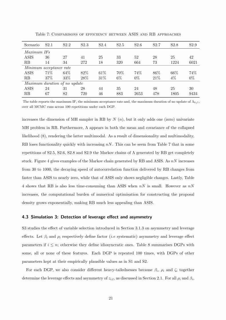
Table 7: Comparisons of efficiency between ASIS and RB approaches
Scenario S2.1 S2.2 S2.3 S2.4 S2.5 S2.6 S2.7 S2.8 S2.9
Maximum IFsASIS 36 27 41 25 33 52 28 25 42RB 14 34 272 18 320 664 73 1224 6021
Minimum acceptance rateASIS 71% 64% 82% 61% 70% 74% 86% 66% 74%RB 37% 33% 28% 31% 6% 0% 21% 4% 0%
Maximum duration of no updateASIS 24 31 28 44 35 24 48 25 30RB 67 82 720 46 883 2653 478 1805 9434
The table reports the maximum IF, the minimum acceptance rate and, the maximum duration of no update of Λk11,
over all MCMC runs across 100 repetitions under each DGP.
increases the dimension of MH sampler in RB by N (n), but it only adds one (zero) univariate
MH problem in RB. Furthermore, Λ appears in both the mean and covariance of the collapsed
likelihood (8), rendering the latter multimodal. As a result of dimensionality and multimodality,
RB loses functionality quickly with increasing nN . This can be seem from Table 7 that in some
repetitions of S2.5, S2.6, S2.8 and S2.9 the Markov chains of Λ generated by RB get completely
stuck. Figure 4 gives examples of the Markov chain generated by RB and ASIS. As nN increases
from 30 to 1000, the decaying speed of autocorrelation function delivered by RB changes from
faster than ASIS to nearly zero, while that of ASIS only shows negligible changes. Lastly, Table
4 shows that RB is also less time-consuming than ASIS when nN is small. However as nN
increases, the computational burden of numerical optimisation for constructing the proposal
density grows exponentially, making RB much less appealing than ASIS.
4.3 Simulation 3: Detection of leverage effect and asymmetry
S3 studies the effect of variable selection introduced in Section 3.1.3 on asymmetry and leverage
effects. Let βi and ρi respectively define factor (i.e systematic) asymmetry and leverage effect
parameters if i ≤ n; otherwise they define idiosyncratic ones. Table 8 summarises DGPs with
some, all or none of these features. Each DGP is repeated 100 times, with DGPs of other
parameters kept at their empirically plausible values as in S1 and S2.
For each DGP, we also consider different heavy-tailednesses because βi, ρi and ζi together
determine the leverage effects and asymmetry of zi,t, as discussed in Section 2.1. For all ρi and βi,
21
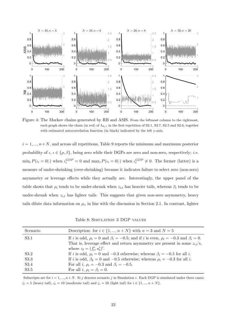
Figure 4: The Markov chains generated by RB and ASIS. From the leftmost column to the rightmost,
each graph shows the chain (in red) of Λk11 in the first repetition of S2.1, S2.7, S2.5 and S2.6, together
with estimated autocorrelation function (in black) indicated by the left y-axis.
i = 1, ..., n+N , and across all repetitions, Table 9 reports the minimum and maximum posterior
probability of ι, ι ∈ ρ, β, being zero while their DGPs are zero and non-zero, respectively; i.e.
mini P (ιi = 0|·) when ιGDPi = 0 and maxi P (ιi = 0|·) when ιGDPi 6= 0. The former (latter) is a
measure of under-shrinking (over-shrinking) because it indicates failure to select zero (non-zero)
asymmetry or leverage effects while they actually are. Interestingly, the upper panel of the
table shows that ρi tends to be under-shrunk when zi,t has heavier tails, whereas βi tends to be
under-shrunk when zi,t has lighter tails. This suggests that given non-zero asymmetry, heavy
tails dilute data information on ρi, in line with the discussion in Section 2.1. In contrast, lighter
Table 8: Simulation 3 DGP values
Scenario Description: for i ∈ 1, ..., n+N with n = 3 and N = 5
S3.1 If i is odd, ρi = 0 and βi = −0.5; and if i is even, ρi = −0.3 and βi = 0.That is, leverage effect and return asymmetry are present in some zi,t’s,where zt = (f ′t , u
′t)′.
S3.2 If i is odd, ρi = 0 and −0.3 otherwise; whereas βi = −0.5 for all i.S3.3 If i is odd, βk = 0 and −0.5 otherwise; whereas ρi = −0.3 for all i.S3.4 For all i, ρi = −0.3 and βi = −0.5.S3.5 For all i, ρi = βi = 0.
Subscripts are for i = 1, ..., n+N . Si.j denotes scenario j in Simulation i. Each DGP is simulated under three cases:
ζi = 5 (heavy tail), ζi = 10 (moderate tail) and ζi = 50 (light tail) for i ∈ 1, ..., n+N.
22
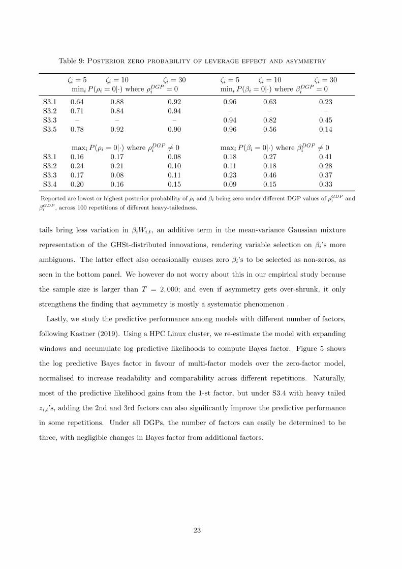
Table 9: Posterior zero probability of leverage effect and asymmetry
ζi = 5 ζi = 10 ζi = 30 ζi = 5 ζi = 10 ζi = 30mini P (ρi = 0|·) where ρDGPi = 0 mini P (βi = 0|·) where βDGPi = 0
S3.1 0.64 0.88 0.92 0.96 0.63 0.23S3.2 0.71 0.84 0.94 – – –S3.3 – – – 0.94 0.82 0.45S3.5 0.78 0.92 0.90 0.96 0.56 0.14
maxi P (ρi = 0|·) where ρDGPi 6= 0 maxi P (βi = 0|·) where βDGPi 6= 0S3.1 0.16 0.17 0.08 0.18 0.27 0.41S3.2 0.24 0.21 0.10 0.11 0.18 0.28S3.3 0.17 0.08 0.11 0.23 0.46 0.37S3.4 0.20 0.16 0.15 0.09 0.15 0.33
Reported are lowest or highest posterior probability of ρi and βi being zero under different DGP values of ρGDPi and
βGDPi , across 100 repetitions of different heavy-tailedness.
tails bring less variation in βiWi,t, an additive term in the mean-variance Gaussian mixture
representation of the GHSt-distributed innovations, rendering variable selection on βi’s more
ambiguous. The latter effect also occasionally causes zero βi’s to be selected as non-zeros, as
seen in the bottom panel. We however do not worry about this in our empirical study because
the sample size is larger than T = 2, 000; and even if asymmetry gets over-shrunk, it only
strengthens the finding that asymmetry is mostly a systematic phenomenon .
Lastly, we study the predictive performance among models with different number of factors,
following Kastner (2019). Using a HPC Linux cluster, we re-estimate the model with expanding
windows and accumulate log predictive likelihoods to compute Bayes factor. Figure 5 shows
the log predictive Bayes factor in favour of multi-factor models over the zero-factor model,
normalised to increase readability and comparability across different repetitions. Naturally,
most of the predictive likelihood gains from the 1-st factor, but under S3.4 with heavy tailed
zi,t’s, adding the 2nd and 3rd factors can also significantly improve the predictive performance
in some repetitions. Under all DGPs, the number of factors can easily be determined to be
three, with negligible changes in Bayes factor from additional factors.
23
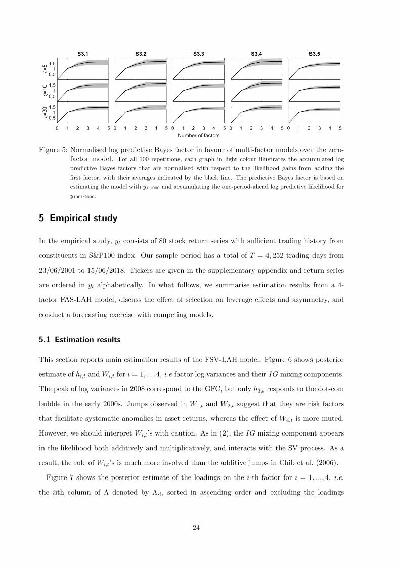
Figure 5: Normalised log predictive Bayes factor in favour of multi-factor models over the zero-factor model. For all 100 repetitions, each graph in light colour illustrates the accumulated log
predictive Bayes factors that are normalised with respect to the likelihood gains from adding the
first factor, with their averages indicated by the black line. The predictive Bayes factor is based on
estimating the model with y1:1000 and accumulating the one-period-ahead log predictive likelihood for
y1001:2000.
5 Empirical study
In the empirical study, yt consists of 80 stock return series with sufficient trading history from
constituents in S&P100 index. Our sample period has a total of T = 4, 252 trading days from
23/06/2001 to 15/06/2018. Tickers are given in the supplementary appendix and return series
are ordered in yt alphabetically. In what follows, we summarise estimation results from a 4-
factor FAS-LAH model, discuss the effect of selection on leverage effects and asymmetry, and
conduct a forecasting exercise with competing models.
5.1 Estimation results
This section reports main estimation results of the FSV-LAH model. Figure 6 shows posterior
estimate of hi,t and Wi,t for i = 1, ..., 4, i.e factor log variances and their IG mixing components.
The peak of log variances in 2008 correspond to the GFC, but only h3,t responds to the dot-com
bubble in the early 2000s. Jumps observed in W1,t and W2,t suggest that they are risk factors
that facilitate systematic anomalies in asset returns, whereas the effect of W4,t is more muted.
However, we should interpret Wi,t’s with caution. As in (2), the IG mixing component appears
in the likelihood both additively and multiplicatively, and interacts with the SV process. As a
result, the role of Wi,t’s is much more involved than the additive jumps in Chib et al. (2006).
Figure 7 shows the posterior estimate of the loadings on the i-th factor for i = 1, ..., 4, i.e.
the iith column of Λ denoted by Λ·i, sorted in ascending order and excluding the loadings
24
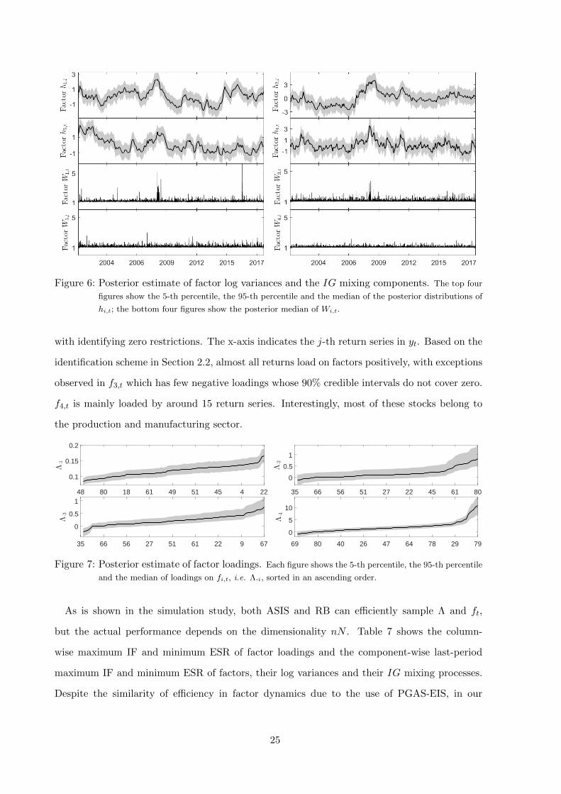
Figure 6: Posterior estimate of factor log variances and the IG mixing components. The top four
figures show the 5-th percentile, the 95-th percentile and the median of the posterior distributions of
hi,t; the bottom four figures show the posterior median of Wi,t.
with identifying zero restrictions. The x-axis indicates the j-th return series in yt. Based on the
identification scheme in Section 2.2, almost all returns load on factors positively, with exceptions
observed in f3,t which has few negative loadings whose 90% credible intervals do not cover zero.
f4,t is mainly loaded by around 15 return series. Interestingly, most of these stocks belong to
the production and manufacturing sector.
48 80 18 61 49 51 45 4 22
0.1
0.15
0.2
35 66 56 51 27 22 45 61 80
0
0.5
1
35 66 56 27 51 61 22 9 67
0
0.5
1
69 80 40 26 47 64 78 29 79
0
5
10
Figure 7: Posterior estimate of factor loadings. Each figure shows the 5-th percentile, the 95-th percentile
and the median of loadings on fi,t, i.e. Λ·i, sorted in an ascending order.
As is shown in the simulation study, both ASIS and RB can efficiently sample Λ and ft,
but the actual performance depends on the dimensionality nN . Table 7 shows the column-
wise maximum IF and minimum ESR of factor loadings and the component-wise last-period
maximum IF and minimum ESR of factors, their log variances and their IG mixing processes.
Despite the similarity of efficiency in factor dynamics due to the use of PGAS-EIS, in our
25
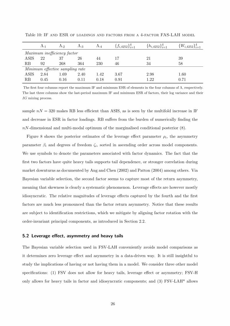
Table 10: IF and ESR of loadings and factors from a 4-factor FAS-LAH model
Λ·1 Λ·2 Λ·3 Λ·4 fi,42524i=1 hi,42524i=1 Wi,42524i=1
Maximum inefficiency factorASIS 22 37 26 44 17 21 39RB 92 268 364 230 46 34 58
Minimum effective sampling rateASIS 2.84 1.69 2.40 1.42 3.67 2.98 1.60RB 0.45 0.16 0.11 0.18 0.91 1.22 0.71
The first four columns report the maximum IF and minimum ESR of elements in the four columns of Λ, respectively.
The last three columns show the last-period maximum IF and minimum ESR of factors, their log variance and their
IG mixing process.
sample nN = 320 makes RB less efficient than ASIS, as is seen by the multifold increase in IF
and decrease in ESR in factor loadings. RB suffers from the burden of numerically finding the
nN -dimensional and multi-modal optimum of the marginalised conditional posterior (8).
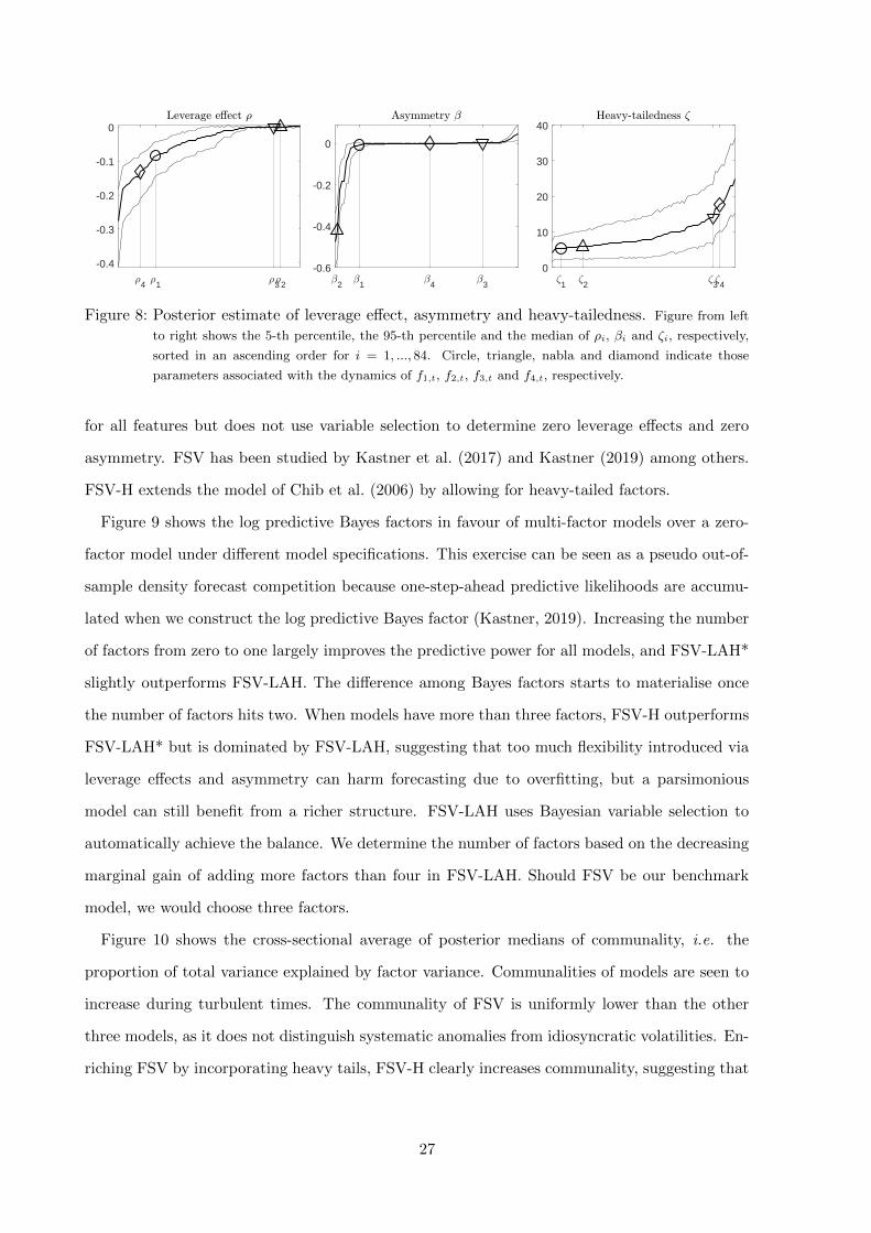
Figure 8 shows the posterior estimates of the leverage effect parameter ρi, the asymmetry
parameter βi and degrees of freedom ζi, sorted in ascending order across model components.
We use symbols to denote the parameters associated with factor dynamics. The fact that the
first two factors have quite heavy tails supports tail dependence, or stronger correlation during
market downturns as documented by Ang and Chen (2002) and Patton (2004) among others. Via
Bayesian variable selection, the second factor seems to capture most of the return asymmetry,
meaning that skewness is clearly a systematic phenomenon. Leverage effects are however mostly
idiosyncratic. The relative magnitudes of leverage effects captured by the fourth and the first
factors are much less pronounced than the factor return asymmetry. Notice that these results
are subject to identification restrictions, which we mitigate by aligning factor rotation with the
order-invariant principal components, as introduced in Section 2.2.
5.2 Leverage effect, asymmetry and heavy tails
The Bayesian variable selection used in FSV-LAH conveniently avoids model comparisons as
it determines zero leverage effect and asymmetry in a data-driven way. It is still insightful to
study the implications of having or not having them in a model. We consider three other model
specifications: (1) FSV does not allow for heavy tails, leverage effect or asymmetry; FSV-H
only allows for heavy tails in factor and idiosyncratic components; and (3) FSV-LAH* allows
26
1 2 3 4
0
10
20
30
40
2 1 4 3
-0.6
-0.4
-0.2
0
4 1 3 2
-0.4
-0.3
-0.2
-0.1
0
Figure 8: Posterior estimate of leverage effect, asymmetry and heavy-tailedness. Figure from left
to right shows the 5-th percentile, the 95-th percentile and the median of ρi, βi and ζi, respectively,
sorted in an ascending order for i = 1, ..., 84. Circle, triangle, nabla and diamond indicate those
parameters associated with the dynamics of f1,t, f2,t, f3,t and f4,t, respectively.
for all features but does not use variable selection to determine zero leverage effects and zero
asymmetry. FSV has been studied by Kastner et al. (2017) and Kastner (2019) among others.
FSV-H extends the model of Chib et al. (2006) by allowing for heavy-tailed factors.
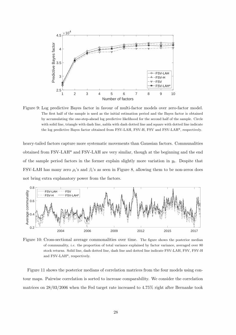
Figure 9 shows the log predictive Bayes factors in favour of multi-factor models over a zero-
factor model under different model specifications. This exercise can be seen as a pseudo out-of-
sample density forecast competition because one-step-ahead predictive likelihoods are accumu-
lated when we construct the log predictive Bayes factor (Kastner, 2019). Increasing the number
of factors from zero to one largely improves the predictive power for all models, and FSV-LAH*
slightly outperforms FSV-LAH. The difference among Bayes factors starts to materialise once
the number of factors hits two. When models have more than three factors, FSV-H outperforms
FSV-LAH* but is dominated by FSV-LAH, suggesting that too much flexibility introduced via
leverage effects and asymmetry can harm forecasting due to overfitting, but a parsimonious
model can still benefit from a richer structure. FSV-LAH uses Bayesian variable selection to
automatically achieve the balance. We determine the number of factors based on the decreasing
marginal gain of adding more factors than four in FSV-LAH. Should FSV be our benchmark
model, we would choose three factors.
Figure 10 shows the cross-sectional average of posterior medians of communality, i.e. the
proportion of total variance explained by factor variance. Communalities of models are seen to
increase during turbulent times. The communality of FSV is uniformly lower than the other
three models, as it does not distinguish systematic anomalies from idiosyncratic volatilities. En-
riching FSV by incorporating heavy tails, FSV-H clearly increases communality, suggesting that
27
1 2 3 4 5 6 7 8 9 10
Number of factors
2.5
3
3.5
4
4.5
Pre
dict
ive
Bay
es fa
ctor
104
FSV-LAHFSV-HFSVFSV-LAH*
Figure 9: Log predictive Bayes factor in favour of multi-factor models over zero-factor model.The first half of the sample is used as the initial estimation period and the Bayes factor is obtained
by accumulating the one-step-ahead log predictive likelihood for the second half of the sample. Circle
with solid line, triangle with dash line, nabla with dash dotted line and square with dotted line indicate
the log predictive Bayes factor obtained from FSV-LAH, FSV-H, FSV and FSV-LAH*, respectively.
heavy-tailed factors capture more systematic movements than Gaussian factors. Communalities
obtained from FSV-LAH* and FSV-LAH are very similar, though at the beginning and the end
of the sample period factors in the former explain slightly more variation in yt. Despite that
FSV-LAH has many zero ρi’s and βi’s as seen in Figure 8, allowing them to be non-zeros does
not bring extra explanatory power from the factors.
2004 2006 2009 2012 2015 20170.2
0.4
0.6
0.8
Ave
rage
com
mun
ality FSV-LAH
FSV-HFSVFSV-LAH*
Figure 10: Cross-sectional average commonalities over time. The figure shows the posterior median
of communality, i.e. the proportion of total variance explained by factor variance, averaged over 80
stock returns. Solid line, dash dotted line, dash line and dotted line indicate FSV-LAH, FSV, FSV-H
and FSV-LAH*, respectively.
Figure 11 shows the posterior medians of correlation matrices from the four models using con-
tour maps. Pairwise correlation is sorted to increase comparability. We consider the correlation
matrices on 28/03/2006 when the Fed target rate increased to 4.75% right after Bernanke took
28
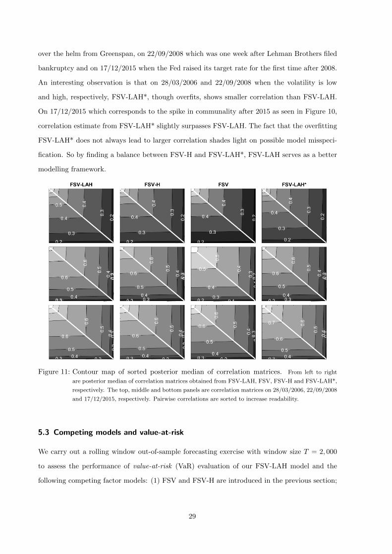
over the helm from Greenspan, on 22/09/2008 which was one week after Lehman Brothers filed
bankruptcy and on 17/12/2015 when the Fed raised its target rate for the first time after 2008.
An interesting observation is that on 28/03/2006 and 22/09/2008 when the volatility is low
and high, respectively, FSV-LAH*, though overfits, shows smaller correlation than FSV-LAH.
On 17/12/2015 which corresponds to the spike in communality after 2015 as seen in Figure 10,
correlation estimate from FSV-LAH* slightly surpasses FSV-LAH. The fact that the overfitting
FSV-LAH* does not always lead to larger correlation shades light on possible model misspeci-
fication. So by finding a balance between FSV-H and FSV-LAH*, FSV-LAH serves as a better
modelling framework.
Figure 11: Contour map of sorted posterior median of correlation matrices. From left to right
are posterior median of correlation matrices obtained from FSV-LAH, FSV, FSV-H and FSV-LAH*,
respectively. The top, middle and bottom panels are correlation matrices on 28/03/2006, 22/09/2008
and 17/12/2015, respectively. Pairwise correlations are sorted to increase readability.
5.3 Competing models and value-at-risk
We carry out a rolling window out-of-sample forecasting exercise with window size T = 2, 000
to assess the performance of value-at-risk (VaR) evaluation of our FSV-LAH model and the
following competing factor models: (1) FSV and FSV-H are introduced in the previous section;
29
(2) CNS (Chib et al., 2006) is a FSV model with heavy tails in the idiosyncratic component ut
and additive jumps that admits a factor structure; (3) FSV-FF is a FSV-LAH model with ft
replaced by three Fama-French (FF) factors (Fama and French, 1993); (4) FSV-FFE stacks FF
factors over yt in the FSV-LAH model and restrict Λ to be such that only (f∗i,t, y′t)′ loads on fi,t
with i = 1, .., 3 and the i-th FF factor f∗i,t; (5) CKL (Chan et al., 1999) is a FSV model with Λ, ft
and ht estimated nonparametrically using rolling windows; (6) DFMG (Santos and Moura, 2014)
is a dynamic factor multivariate GARCH model that uses FF factors with volatility extracted
from a GARCH model and time-varying loadings estimated by Kalman filter conditional on
GARCH volatility; (7) FCO (Oh and Patton, 2017) is a factor copula model with marginals
estimated from GARCH models and a copula implied by a static Gaussian 2-factor model; (8)
FCOt is the same as FCO but with GARCHt marginals.
For each s ∈ 2001, ..., 4252 − h, we simulate 104 h-step-ahead return vectors ys+h|s, to
construct the empirical predictive distribution of the portfolio Fs+h|s(y). The h-step-ahead VaR
at nominal level α is forecast by VaRs+h|s(α) = F−1s+h|s(α). For various FSV models and CNS,
ys+1, ..., ys+h are generated conditional on parameter vector θ simulated from the posterior. For
other models, we keep θ is at its maximum likelihood estimate and derive Fs+h|s(y) recursively.
We define a hit process such that Ih,s(α) = 1 if (1/N)∑N
i=1 yi,s+h|s < VaRs+h|s(α) and 0
otherwise. Well-behaved VaR forecasts should deliver a serially independent Ih,s(α), Ih,s(α) ⊥
Ih,s−1(α) in particular, and has correct unconditional coverage ratio, i.e. P (Is(h, α) = 1) =
E(Is(h, α)) = α (Lopez and Walter, 2001). Based on Ih,s(α) and hit rate (HR), or the sam-
ple average of Is(h, α), Christoffersen (1998) develops likelihood ratio tests – LRind for serial
independence, LRuc for unconditional coverage and LRcc for conditional coverage.
Table 11 summarises test results when h ∈ 1, 5 and α ∈ 0.01, 0.05. Not surprisingly, FSV-
LAH uniformly outperforms FSV. The result suggests that modelling leverage effects, return
asymmetry and heavy tails brings in forecasting power for financial returns. This can also
be seen if we compare FCOt which incorporates Student’s t marginals with FCO. However,
comparing both FSV-H and FSV-LAH* with FSV-LAH when h = 5 or α = 0.01 suggests that
Bayesian variable selection embedded in the latter model improves forecasting by balancing
parsimony and flexibility. Furthermore, compared with FSV-LAH, CNS performs equally well
when h = 1, but poorer when h = 5. To explain this, we notice that CNS uses additive jumps
30
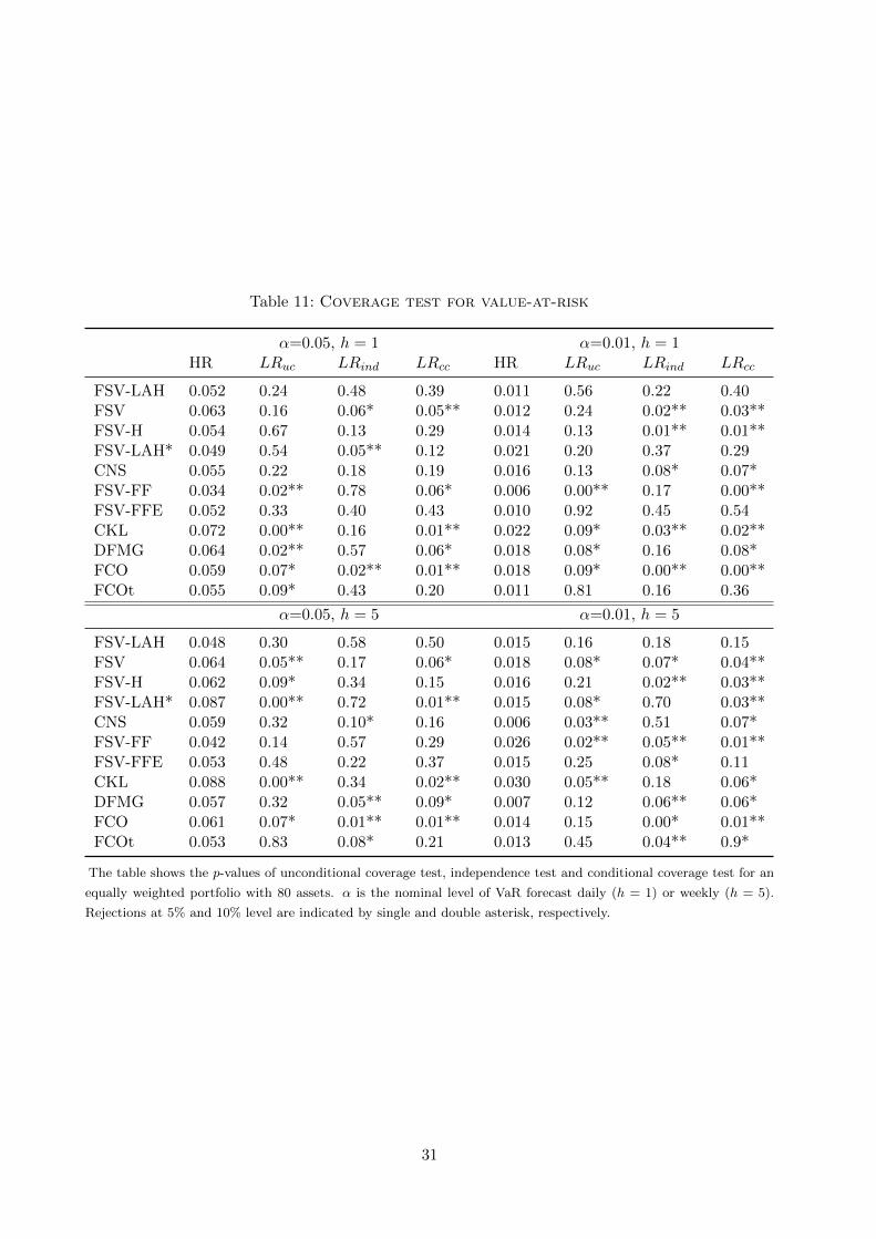
Table 11: Coverage test for value-at-risk
α=0.05, h = 1 α=0.01, h = 1HR LRuc LRind LRcc HR LRuc LRind LRcc
FSV-LAH 0.052 0.24 0.48 0.39 0.011 0.56 0.22 0.40FSV 0.063 0.16 0.06* 0.05** 0.012 0.24 0.02** 0.03**FSV-H 0.054 0.67 0.13 0.29 0.014 0.13 0.01** 0.01**FSV-LAH* 0.049 0.54 0.05** 0.12 0.021 0.20 0.37 0.29CNS 0.055 0.22 0.18 0.19 0.016 0.13 0.08* 0.07*FSV-FF 0.034 0.02** 0.78 0.06* 0.006 0.00** 0.17 0.00**FSV-FFE 0.052 0.33 0.40 0.43 0.010 0.92 0.45 0.54CKL 0.072 0.00** 0.16 0.01** 0.022 0.09* 0.03** 0.02**DFMG 0.064 0.02** 0.57 0.06* 0.018 0.08* 0.16 0.08*FCO 0.059 0.07* 0.02** 0.01** 0.018 0.09* 0.00** 0.00**FCOt 0.055 0.09* 0.43 0.20 0.011 0.81 0.16 0.36
α=0.05, h = 5 α=0.01, h = 5
FSV-LAH 0.048 0.30 0.58 0.50 0.015 0.16 0.18 0.15FSV 0.064 0.05** 0.17 0.06* 0.018 0.08* 0.07* 0.04**FSV-H 0.062 0.09* 0.34 0.15 0.016 0.21 0.02** 0.03**FSV-LAH* 0.087 0.00** 0.72 0.01** 0.015 0.08* 0.70 0.03**CNS 0.059 0.32 0.10* 0.16 0.006 0.03** 0.51 0.07*FSV-FF 0.042 0.14 0.57 0.29 0.026 0.02** 0.05** 0.01**FSV-FFE 0.053 0.48 0.22 0.37 0.015 0.25 0.08* 0.11CKL 0.088 0.00** 0.34 0.02** 0.030 0.05** 0.18 0.06*DFMG 0.057 0.32 0.05** 0.09* 0.007 0.12 0.06** 0.06*FCO 0.061 0.07* 0.01** 0.01** 0.014 0.15 0.00* 0.01**FCOt 0.053 0.83 0.08* 0.21 0.013 0.45 0.04** 0.9*
The table shows the p-values of unconditional coverage test, independence test and conditional coverage test for an
equally weighted portfolio with 80 assets. α is the nominal level of VaR forecast daily (h = 1) or weekly (h = 5).
Rejections at 5% and 10% level are indicated by single and double asterisk, respectively.
31
for return anomalies in yt, whereas FSV-LAH features both additive and multiplicative swings
modelled by the IG mixing components, which also interact with the SV processes. Lastly, FSV-
FF, DFMG and CKL replace ft with observed FF factors. Though the former two are quite
flexible, the fact that they are outperformed by FSV-LAH and FSV-FFE may suggest that
signals in FF factors are eclipsed by their noises, leading to inaccuracy and misspecification.
Interestingly, FSV-LAH and FSV-FFE perform comparably well. This result indicates that FF
factors do not bring extra information in forecasting VaR in our sample, and how factors are
loaded is of secondary importance.
6 Conclusion and remarks
Advances in Monte Carlo methods such as the efficient importance sampling (EIS) algorithm
of Richard and Zhang (2007) and the particle Gibbs method of Andrieu et al. (2010) allow us
to design efficient MCMC algorithms for the estimation of flexible factor stochastic volatility
models in many dimensions. Our framework connects findings in empirical literature that doc-
uments commonality in the third moments of financial returns and higher pairwise correlations
during market downturns to the literature on multivariate financial time series that aims to
address the curse of dimensionality and overcome computational challenges towards the estima-
tion of increasingly more accurate models. Extensions of the current model include exploring
coupled systems of smaller subsets of yt within each set PGAS-EIS can deliver better posterior
approximation. This can be approached using the framework of simultaneous graphical dynamic
linear models proposed by Gruber et al. (2016). Also, it will be interesting to combine our
sampling algorithm with the order-invariant formulation of factor models in Chan et al. (2018)
and Kaufmann and Schumacher (2019) and study the effect order dependence has on forecast-
ing covariance matrix. Lastly, our empirical study reveals that some factors are loaded by only
a subset of assets. The sparse loading matrix of Kastner (2019) can be directly implemented
within our framework to maintain a more parsimonious model specification.
References
Aas, K. and I. H. Haff (2006). The generalized hyperbolic skew Student’s t-distribution. Journalof Financial Econometrics 4 (2), 275–309.
32
Aguilar, O. and M. West (2000). Bayesian dynamic factor models and portfolio allocation.Journal of Business & Economic Statistics 18 (3), 338–357.
Andrieu, C., A. Doucet, and R. Holenstein (2010). Particle markov chain monte carlo methods.Journal of the Royal Statistical Society: Series B (Statistical Methodology) 72 (3), 269–342.
Andrieu, C. and G. Roberts (2009). The pseudo-marginal approach for efficient monte carlocomputations. The Annals of Statistics 37 (2), 697–725.
Ang, A. and J. Chen (2002). Asymmetric correlations of equity portfolios. Journal of financialEconomics 63 (3), 443–494.
Asai, M., M. McAleer, and J. Yu (2006). Multivariate stochastic volatility: a review. Econo-metric Reviews 25 (2-3), 145–175.
Bai, J. and P. Wang (2015). Identification and Bayesian estimation of dynamic factor models.Journal of Business & Economic Statistics 33 (2), 221–240.
Beine, M., A. Cosma, and R. Vermeulen (2010). The dark side of global integration: Increasingtail dependence. Journal of Banking & Finance 34 (1), 184–192.
Chan, J., R. Leon-Gonzalez, and R. W. Strachan (2018). Invariant inference and efficient com-putation in the static factor model. Journal of the American Statistical Association 113 (522),819–828.
Chan, L. K., J. Karceski, and J. Lakonishok (1999). On portfolio optimization: Forecastingcovariances and choosing the risk model. Review of Financial Studies 12 (5), 937–974.
Chib, S. (2001). Markov chain Monte Carlo methods: computation and inference. Handbook ofeconometrics 5, 3569–3649.
Chib, S., F. Nardari, and N. Shephard (2006). Analysis of high dimensional multivariate stochas-tic volatility models. Journal of Econometrics 134 (2), 341–371.
Chib, S., Y. Omori, and M. Asai (2009). Multivariate stochastic volatility. In Handbook ofFinancial Time Series, pp. 365–400. Springer.
Chopin, N., S. S. Singh, et al. (2013). On the particle Gibbs sampler. CREST.
Christoffersen, P. F. (1998). Evaluating interval forecasts. International economic review , 841–862.
Clyde, M. and E. I. George (2004). Model uncertainty. Statistical science, 81–94.
Dang, D.-M., K. R. Jackson, and M. Mohammadi (2015). Dimension and variance reductionfor Monte Carlo methods for high-dimensional models in finance. Applied Mathematical Fi-nance 22 (6), 522–552.
Doornik, J. A. (2007). Object-Oriented Matrix Programming Using Ox, 3rd ed. London: Tim-berlake Consultants Press.
Doucet, A., N. De Freitas, and N. Gordon (2001). An introduction to sequential Monte Carlomethods. In Sequential Monte Carlo methods in practice, pp. 3–14. Springer.
Durbin, J. and S. J. Koopman (1997). Monte Carlo maximum likelihood estimation for non-gaussian state space models. Biometrika 84 (3), 669–684.
Fama, E. F. and K. R. French (1993). Common risk factors in the returns on stocks and bonds.Journal of financial economics 33 (1), 3–56.
Geweke, J. and H. Tanizaki (2001). Bayesian estimation of state-space models using theMetropolis–Hastings algorithm within Gibbs sampling. Computational Statistics & Data Anal-ysis 37 (2), 151–170.
Gilks, W. R., N. Best, and K. Tan (1995). Adaptive rejection Metropolis sampling within Gibbssampling. Applied Statistics, 455–472.
Grothe, O., T. S. Kleppe, and R. Liesenfeld (2017). The gibbs sampler with particle efficient
33
importance sampling for state-space models.
Gruber, L., M. West, et al. (2016). GPU-accelerated Bayesian learning and forecasting insimultaneous graphical dynamic linear models. Bayesian Analysis 11 (1), 125–149.
Gruber, L., M. West, et al. (2017). Bayesian forecasting and portfolio decisions using simulta-neous graphical dynamic linear models. Econometrics and Statistics 3, 3–22.
Hosszejni, D. and G. Kastner (2019). Approaches toward the Bayesian estimation of the stochas-tic volatility model with leverage. Bayesian Statistics and New Generations, 75.
Jacquier, E., N. G. Polson, and P. E. Rossi (2004). Bayesian analysis of stochastic volatilitymodels with fat-tails and correlated errors. Journal of Econometrics 122 (1), 185–212.
Jung, R. C. and R. Liesenfeld (2001). Estimating time series models for count data using efficientimportance sampling. AStA Advances in Statistical Analysis 4 (85), 387–407.
Kastner, G. (2019). Sparse Bayesian time-varying covariance estimation in many dimensions.Journal of Econometrics 210 (1), 98–115.
Kastner, G. and S. Fruhwirth-Schnatter (2014). Ancillarity-sufficiency interweaving strategy(ASIS) for boosting MCMC estimation of stochastic volatility models. Computational Statis-tics & Data Analysis 76, 408–423.
Kastner, G., S. Fruhwirth-Schnatter, and H. F. Lopes (2017). Efficient Bayesian inferencefor multivariate factor stochastic volatility models. Journal of Computational and GraphicalStatistics 26 (4), 905–917.
Kaufmann, S. and C. Schumacher (2019). Bayesian estimation of sparse dynamic factor modelswith order-independent and ex-post mode identification. Journal of Econometrics 210 (1),116–134.
Kim, S., N. Shephard, and S. Chib (1998). Stochastic volatility: likelihood inference and com-parison with ARCH models. The Review of Economic Studies 65 (3), 361–393.
Koop, G., D. J. Poirier, and J. L. Tobias (2007). Bayesian econometric methods. CambridgeUniversity Press.
Koopman, S. J. and E. Hol Uspensky (2002). The stochastic volatility in mean model: empiricalevidence from international stock markets. Journal of applied Econometrics 17 (6), 667–689.
Koopman, S. J., N. Shephard, and J. A. Doornik (2008). SsfPack 3.0: Statistical algorithms formodels in state space form. London: Timberlake Consultants Press.
Kurose, Y. and Y. Omori (2016). Dynamic equicorrelation stochastic volatility. ComputationalStatistics & Data Analysis 100, 795–813.
Lindsten, F., M. I. Jordan, and T. B. Schon (2014). Particle gibbs with ancestor sampling.Journal of Machine Learning Research 15 (1), 2145–2184.
Lopez, J. A. and C. A. Walter (2001). Evaluating covariance matrix forecasts in a value-at-riskframework. The Journal of Risk 3, 69–97.
Nakajima, J. (2017). Bayesian analysis of multivariate stochastic volatility with skew returndistribution. Econometric Reviews 36 (5), 546–562.
Nakajima, J. and Y. Omori (2012). Stochastic volatility model with leverage and asymmetricallyheavy-tailed error using GH skew Student’s t-distribution. Computational Statistics & DataAnalysis 56 (11), 3690–3704.
Nelson, D. B. (1991). Conditional heteroskedasticity in asset returns: A new approach. Econo-metrica: Journal of the Econometric Society , 347–370.
Oh, D. H. and A. J. Patton (2017). Modeling dependence in high dimensions with factor copulas.Journal of Business & Economic Statistics 35 (1), 139–154.
Patton, A. J. (2004). On the out-of-sample importance of skewness and asymmetric dependencefor asset allocation. Journal of Financial Econometrics 2 (1), 130–168.
34
Pitt, M. and N. Shephard (1999a). Time varying covariances: a factor stochastic volatilityapproach. Bayesian statistics 6, 547–570.
Pitt, M. K., R. dos Santos Silva, P. Giordani, and R. Kohn (2012). On some properties ofMarkov chain Monte Carlo simulation methods based on the particle filter. Journal of Econo-metrics 171 (2), 134–151.
Pitt, M. K. and N. Shephard (1999b). Filtering via simulation: Auxiliary particle filters. Journalof the American statistical association 94 (446), 590–599.
Richard, J.-F. and W. Zhang (2007). Efficient high-dimensional importance sampling. Journalof Econometrics 141 (2), 1385–1411.
Santos, A. A. and G. V. Moura (2014). Dynamic factor multivariate garch model. ComputationalStatistics & Data Analysis 76, 606–617.
Scharth, M. and R. Kohn (2016). Particle efficient importance sampling. Journal of Economet-rics 190 (1), 133–147.
Shephard, N. and M. K. Pitt (1997). Likelihood analysis of non-gaussian measurement timeseries. Biometrika 84 (3), 653–667.
Snyder, C., T. Bengtsson, P. Bickel, and J. Anderson (2008). Obstacles to high-dimensionalparticle filtering. Monthly Weather Review 136 (12), 4629–4640.
Watanabe, T. and Y. Omori (2004). A multi-move sampler for estimating non-gaussian timeseries models: Comments on shephard & pitt (1997). Biometrika, 246–248.
Yu, J. (2005). On leverage in a stochastic volatility model. Journal of Econometrics 127 (2),165–178.
Yu, Y. and X.-L. Meng (2011). To center or not to center: That is not the question—Anancillarity–sufficiency interweaving strategy (ASIS) for boosting MCMC efficiency. Journalof Computational and Graphical Statistics 20 (3), 531–570.
35