1

LEXICAL DIFFERENCES BETWEEN TUSCAN DIALECTS AND

STANDARD ITALIAN: A SOCIOLINGUISTIC ANALYSIS USING

GENERALIZED ADDITIVE MIXED MODELING

Martijn Wielinga, Simonetta Montemagni

b, John Nerbonne

c and R. Harald Baayen

a,d

aDepartment of General Linguistics, University of Tübingen, Germany,

bIstituto di Linguistica

Computationale “Antonio Zampolli”, CNR, Italy, cDepartment of Humanities Computing, University

of Groningen, the Netherlands, and dDepartment of Linguistics, University of Alberta, Canada

wieling@gmail.com, simonetta.montemagni@ilc.cnr.it, j.nerbonne@rug.nl, harald.baayen@uni-

tuebingen.de

Abstract

This study uses a generalized additive mixed-effects regression model to predict lexical differences in

Tuscan dialects with respect to standard Italian. We used lexical information for 170 concepts used by

2060 speakers in 213 locations in Tuscany. In our model, geographical position was found to be an

important predictor, with locations more distant from Florence having lexical forms more likely to

differ from standard Italian. In addition, the geographical pattern varied significantly for low versus

high frequency concepts and older versus younger speakers. Younger speakers generally used variants

more likely to match the standard language. Several other factors emerged as significant. Male speakers

as well as farmers were more likely to use a lexical form different from standard Italian. In contrast,

higher educated speakers used lexical forms more likely to match the standard. The model also

indicates that lexical variants used in smaller communities are more likely to differ from standard

Italian. The impact of community size, however, varied from concept to concept. For a majority of

concepts, lexical variants used in smaller communities are more likely to differ from the standard

Italian form. For a minority of concepts, however, lexical variants used in larger communities are more

likely to differ from standard Italian. Similarly, the effect of the other community- and speaker-related

predictors varied per concept. These results clearly show that the model succeeds in teasing apart

different forces influencing the dialect landscape and helps us to shed light on the complex interaction

between the standard Italian language and the Tuscan dialectal varieties. In addition, this study

illustrates the potential of generalized additive mixed-effects regression modeling applied to dialect

data.

Key words

Tuscan dialects, Lexical variation, Generalized additive modeling, Mixed-effects regression modeling

2

1. Introduction

In spite of their different origin and history, it is nowadays a widely acknowledged

fact that traditional dialectology (to be understood here as dialect geography) and

sociolinguistics (or urban dialectology) can be seen as two streams of a unique and

coherent discipline: modern dialectology (Chambers and Trudgill, 1998). Chambers

and Trudgill (1998:187-188) describe the convergence of these two historically

separated disciplines as follows:

For all their differences, dialectology and sociolinguistics converge at their

deepest point. Both are dialectologies, so to speak. They share their essential

subject matter. Both fix the attention on language in communities.

Prototypically, one has been centrally concerned with rural communities and

the other with urban centres, but these are accidental differences, not essential

ones and certainly not axiomatic. […] A decade or two ago, it might have been

possible to think that the common subject matter of dialectology and

sociolinguistics counted for next to nothing. Now we know it counts for

everything.

In practice, however, dialectology and sociolinguistics remain separate fields when

considering the methods and techniques used for analyzing language variation and

change.

Sociolinguistics - whose basic goal consists of identifying the social factors

underlying the use of different variants of linguistic variables - adopted a quantitative

approach to data analysis since its inception (e.g., Labov, 1966). Over time, different

methods for the analysis of linguistic variation were developed, capable of modeling

the joint effect of an increasing number of factors related to the social background of

speakers (including age, gender, socio-economic status, etc.) and linguistic features.

While early studies focused on simple relationships between the value of a linguistic

variable and the value of a social variable (see e.g. Labov, 1966, 1972), over time

more advanced statistical methods for the analysis of linguistic variation were

developed. Since the 1970s, the most common method in sociolinguistic research has

been logistic regression (Cedergren and Sankoff, 1974) and more recently, mixed-

3

effects regression models have been applied to socio-linguistic data (Johnson, 2009;

Tagliamonte and Baayen, 2012, Wieling et al., 2011).

Traditional dialectology shows a different pattern. Since its origin in the second half

of the 19th century, it typically relied on the subjective analysis of categorical maps

charting the distribution of the different variants of a linguistic variable across a

region. Only later, i.e. during the last forty years, quantitative methods have been

applied to the analysis of dialect variation. This quantitative approach to the study of

dialects is known as dialectometry (Séguy, 1973; Goebl, 1984, 2006; Nerbonne et al.,

1996; Nerbonne, 2003; Nerbonne and Kleiweg, 2007). Dialectometric methods focus

mostly on identifying the most important dialectal groups (i.e. in terms of geography)

using an aggregate analysis of the linguistic data. The aggregate analysis is based on

computing the distance (or similarity) between every pair of locations in the dataset

based on the complete set of linguistic variables and by analyzing the resulting

linguistic distance (or similarity) matrix using multivariate statistics to identify

aggregate geographical patterns of linguistic variation.

While viewing dialect differences at an aggregate level arguably provides a more

comprehensive and objective view than the analysis of a small number of subjectively

selected features (Nerbonne, 2009), the aggregate approach has never fully convinced

linguists of its use as it fails to identify the linguistic basis of the identified groups

(see e.g. Loporcaro, 2009). By initially aggregating the values of numerous linguistic

variables, traditional dialectometric analyses offer no direct method for testing

whether and to what extent an individual linguistic variable contributes to observed

patterns of variation. Recent developments in dialectometric research tried to reduce

the gap between models of linguistic variation based on quantitative analyses and

more traditional analyses based on specific linguistic features. Wieling and Nerbonne

(2010, 2011) proposed a new dialectometric method, the spectral partitioning of

bipartite graphs, to cluster linguistic varieties and simultaneously determine the

underlying linguistic basis. This method, originally applied to Dutch dialects, was also

successfully tested on English (Wieling et al., 2013) and Tuscan (Montemagni et al.,

2012) dialects. Unfortunately, these methods still disregard social factors, and only

take into account the influence of geography.

4

While some attempts have been made, social and spatial analyses of language are still

far from being integrated. Britain (2002) reports that sociolinguistics fails to

incorporate the notion of spatiality in its research. On the other hand, dialectometry

mainly focuses on dialect geography and generally disregards social factors. The few

exceptions indeed “prove” the proverbial rule. Montemagni et al. (2013) and Valls et

al. (2013) included in their dialectometric analyses social factors concerning the

difference between age classes or urban versus rural communities. Unfortunately, the

effect of these social factors was evaluated by simply comparing maps visually, as

opposed to statistically testing the differences. Another relevant aspect on which the

sociolinguistic and dialectometric perspectives do not coincide concerns the role of

individual features, which are central in sociolinguistics, but are typically and

programmatically disregarded in dialectometry. These issues demonstrate that there is

an increasing need for statistical methods capable of accounting for both the

geographic and socio-demographic variation, as well as for the impact and role of

individual linguistic features.

The present study is methodologically ambitious for its attempt to combine

dialectometric and sociolinguistic perspectives along the lines depicted above. The

statistical analysis methods we employ enable the incorporation of candidate

explanatory variables based on social, geographical as well as linguistic factors,

making it a good technique to facilitate the intellectual merger of dialectology and

sociolinguistics (Wieling, 2012). The starting point is the study by Wieling, Nerbonne

and Baayen (2011) who proposed a novel method using a generalized additive model

in combination with a mixed-effects regression approach to simultaneously account

for the effects of geographical, social and linguistic variables. They used a basic

generalized additive model to represent the global geographical pattern, which was

used in a second step as a predictor in their linear mixed-effects regression model.

Their model predicted word pronunciation distances from the standard language to

424 Dutch dialects and it turned out that both the geographical location of the

communities, as well as several location-related predictors (i.e. community size and

average community age) and word-related factors (i.e. word frequency and category)

were significant predictors. While the study of Wieling et al. (2011) includes social,

lexical and geographical information, a drawback of their study is that they only

5

considered a single speaker per location, limiting the potential influence of speaker-

related variables.

In this paper, we present an extended analytical framework which was tested on an

interesting case study: Tuscan lexical variation with respect to standard Italian. There

are three clear and important differences with respect to the study of Wieling et al.

(2011). First, since the software available for generalized additive mixed-effects

regression modeling has improved significantly since the study of Wieling et al.

(2011), we are able to advance on their approach by constructing a single generalized

additive mixed-effects regression model. This is especially beneficial as we are now

in a position to better assess the effect of concept frequency, a variable which has

largely been ignored from dialectological studies, but is highly relevant as it “[...] may

affect the rate at which new words arise and become adopted in populations of

speakers” (Pagel et al., 2007). Second, in this study we focus on lexical variation

rather than variation in pronunciation. We therefore do not try to predict dialect

distances, but rather a binary value indicating whether the lexicalization of a concept

is different (1) or equal (0) with respect to standard Italian. A benefit of this approach

is that it is more in line with standard sociolinguistic practice, which also focuses on

binary distinctions. Third, as we take into account multiple speakers per location, we

are at an improved position to investigate the contribution of speaker-related variables

such as age and gender.

The Tuscan dialect case study we use to investigate the potential of this new method

(integrating social, geographical and lexical factors) is a challenging one. In Italy a

complex relationship exists between the standard language and dialects due to the

history of this language and the circumstances under which Italy achieved political

unification in 1861, much later than in most European countries. In Tuscany, a region

with a special status among Italian dialects, the situation is even more complex as

standard Italian is based on Tuscan, and in particular on the Florentine variety, which

achieved national and international prestige from the fourteenth century onwards as a

literary language and only later (after the Italian Unification, and mainly in the

twentieth century) as a spoken language. However, standard Italian has never been

identical to genuine Tuscan and is perhaps best described as an “abstraction”

increasingly used for general communication purposes. The aim of this study,

6

therefore, is to investigate this particular relationship between Italian and Tuscan

dialects. We focus on lexical variation in Tuscan dialects compared to standard Italian

with the goal of defining the impact, role and interaction of a wide range of factors

(i.e. social, lexical and geographical) in determining lexical choice by Tuscan dialect

speakers. The study is based on a large set of dialect data, i.e. the lexicalizations of

170 concepts attested by 2060 speakers in 213 Tuscan varieties drawn from the corpus

of dialectal data Atlante Lessicale Toscano (‘Lexical Atlas of Tuscany’, henceforth

ALT; Giacomelli et al., 2000) in which lexical data have both a diatopic and diastratic

characterization.

After discussing the special relationship between standard Italian and the Tuscan

dialects in the next section, we will describe the Tuscan dialect dataset, followed by a

more in-depth explanation of the generalized additive modeling procedure, our results

and the implications of our findings.

2. Tuscan dialects and standard Italian

2.1. The notions of dialect and standard language in the Italian context

As pointed out by Berruto (2005), Italy’s dialetti do not correspond to the same entity

as e.g., the English dialects. Following the Coserian distinction among primary,

secondary and tertiary dialects (Coseriu, 1980), the Italian dialects are to be

understood as primary dialects, i.e. dialects having their own autonomous linguistic

system, whereas the English dialects represent tertiary dialects, i.e. varieties resulting

from the social and/or geographical differentiation of the standard language. Italian

dialects – or, more technically, Italo-Romance varieties – thus do not represent

varieties of Italian but independent ‘sister’ languages arisen from local developments

of Latin (Maiden, 1995).

A similar ‘sisterhood’ relationship also exists between the Italian language and Italo-

Romance dialects, because Italian has its roots in one of the speech varieties that

emerged from spoken Vulgar Latin (Maiden and Parry, 1997), namely that of

Tuscany, and more precisely the variety of Tuscan spoken in Florence. The

importance of the Florentine variety in Italy was mainly determined by the prestige of

7

the Florentine culture, and in particular the establishment of Dante, Petrarch and

Boccaccio, who wrote in Florentine, as the ‘three crowns’ (tre corone) of Italian

literature. The fact that standard Italian originated from the Florentine dialect

centuries ago changes the type of relationship between standard Italian and Tuscan

dialects to a kind of ‘parental’ relationship instead of a ‘sisterhood’ relationship.

Clearly, this complicates matters with respect to the relationship between the Tuscan

dialects and the standard Italian language, and this is the topic of the present study.

Standard Italian is unique among modern European standard languages. Even though

it originated in the fourteenth century, it was not consolidated as a spoken national

language until the twentieth century. For centuries, Italian was a written literary

language, acquired through literacy when one learned to read and write, and was

therefore only known to a minority of (literate) people. During this period, people

spoke only their local dialect. For a detailed account of the rise of standard Italian the

interested reader is referred to e.g. Migliorini and Griffith (1984). The particular

nature of Italian as a literary language, rather than a spoken language, was recognized

since its origin and has been widely debated from different (i.e. socio-economic,

political and cultural) perspectives under the general heading of questione della lingua

or ‘language question’.

At the time of the Italian political unification in 1861 only a very small percentage of

the population was able to speak Italian, with estimates ranging from 2.5% (De

Mauro, 1963) to 10% (Castellani, 1982). Only during the second half of the 20th

century real native speakers of Italian started to appear, as Italian started to be used by

Italians as a spoken language in everyday life. Mass media (newspapers, radio and

TV), education, and the introduction of compulsory military service played a central

role in the diffusion of the Italian language throughout the country. According to

recent statistics by the Italian National Census (Istituto Nazionale di Statistica,

ISTAT) reported by Lepschy (2002), 98% of the Italian population is able to use their

national language. However, dialects and standard Italian continue to coexist. For

example, ISTAT data show that at the end of the 20th century (1996) 50% of the

population used (mainly or exclusively) standard Italian to communicate with friends

and colleagues, while this percentage decreased to 34% when communication with

relatives was taken into account. More recently, Dal Negro and Vietti (2011)

8

presented a quantitative analysis of the patterns of language choice in present-day

Italy on the basis of a national survey carried out by ISTAT in 2006. At the national

level, they reported that 45.5% exclusively used Italian in a family setting, whereas

32.5% of the people alternated between dialectal and Italian speech, and 16%

exclusively spoke in dialect (with the remaining ones using another language).

The current sociolinguistic situation of Italy is characterized by the presence of

regional varieties of Italian (e.g., Berruto, 1989, 2005; Cerutti, 2011). Following the

tripartite Coserian classification of dialects, these can be seen as tertiary dialects, i.e.

varieties of the standard language that are spoken in different geographical areas.

They differ both from each other and from standard Italian at all levels (phonetic,

prosodic, syntactic and lexical), and represent the Italian actually spoken in

contemporary Italy. Common Italian speakers generally speak a regional variety of

Italian, referred to as regional Italian. The consequence of this is that there are no real

native speakers of standard Italian. Not even a Tuscan or Florentine native speaker

could be considered a native speaker of standard Italian, as in Tuscan or Florentine

Italian features exist (such as the well-known Tuscan gorgia) which are not part of the

standard Italian norm.

This clearly raises the question of what we mean by the standard Italian language.

Generally speaking, a standard language is a fuzzy notion. Following Ammon (2004),

the standard variety of a language can be seen as having a core of undoubtedly

standard forms while also having fuzzy boundaries resulting in a complex gradation

between standard and non-standard. In Italy, a new standard variety “neo-standard

Italian” (Berruto, 1987) is emerging as the result of a restandardization process, which

allows for a certain amount of regional differentiation. For the specific concerns of

this study, aimed at reconstructing the factors governing the lexical choices of Tuscan

speakers between dialect and standard language, we will refer to the core of

undoubtedly standard forms as standard Italian. This is the only way to avoid

interferences with the regional Italian spoken in Tuscany.

9

2.2. Previous studies on the relationship between standard Italian and Tuscan

dialects

The specific relationship linking standard Italian and Tuscan dialects has been

investigated in numerous studies. Given the goal of our research, we will only discuss

those studies which focus on the lexical level.

The historical link between the Tuscan dialects and the standard Italian language

causes frequent overlap between dialectal and standard lexical forms in Tuscany, and

less frequent overlap in other Italian regions (Giacomelli, 1978). However, since

Tuscan dialects have developed (for several centuries) along their own lines and

independently of the (literary) standard Italian language, their vocabulary does not

always coincide with that of standard Italian. Following Giacomelli (1975), the types

of mismatch between standard Italian and the dialectal forms can be partitioned into

three groups. The first group consists of Tuscan words which are used in literature

throughout Italy, but are not part of the standard language (i.e. these terms usually

appear in Italian dictionaries marked as ‘Tuscanisms’). The second group consists of

Tuscan words which were part of old Italian and are also attested in the literature

throughout Italy, but have fallen into disuse as they are considered old-fashioned (i.e.

these terms may appear in Italian dictionaries marked as ‘archaisms’). The final group

consists of Tuscan dialectal words which have no literary tradition and are not

understood outside of Tuscany.

Here our goal is to investigate the complex relationship between standard Italian and

the Tuscan dialects from which it originated on the basis of the data collected through

fieldwork for the Atlante Lessicale Toscano (ALT). Previous studies have already

explored the ALT dataset by investigating the relationship between Tuscan and Italian

from the lexical point of view. Giacomelli and Poggi Salani (1984) based their

analysis on the dialect data available at that time. Montemagni (2008), more recently,

applied dialectometric techniques to the whole ALT dialectal corpus to investigate the

relationship between Tuscan and Italian. In both cases it turned out that the Tuscan

dialects overlap most closely with standard Italian in the area around Florence,

expanding in different directions and in particular towards the southwest. Obviously,

this observed synchronic pattern of lexical variation has the well-known diachronic

10

explanation that the standard Italian language originated from the Florentine variety of

Tuscan.

Montemagni (2008) also found that the observed patterns varied depending on the

speaker’s age: only 37 percent of the dialectal answers of the old speakers (i.e. born in

1920 or before) overlapped with standard Italian, while this percentage increased to

44 for the young speakers (i.e. born after 1945, when standard Italian started being

progressively used). In addition, words having a larger geographical coverage (i.e. not

specific to a small region), were more likely to coincide with the standard language

than words attested in smaller areas. These first, basic results illustrate the potential of

the ALT dataset (which we use here as well, and will be discussed in more detail in

Section 3.1) to shed light on the complex relationship between standard Italian and

Tuscan dialects.

3. Material

3.1. Lexical data

The lexical data used in this study was taken from the Atlante Lessicale Toscano

(ALT), a specially designed regional atlas in which the dialectal data have a diatopic

(geographic), diastratic (social) and diachronic characterization. The diachronic

characterization covers only a few generations whose year of birth ranges from the

end of the 19th century to the second half of the 20th century. It is interesting to note

that only the younger ALT informants were born in the period when standard Italian

started being used as a spoken language. ALT interviews were carried out between

1974 and 1986 in 224 localities of Tuscany. The localities were hierarchically

organized according to their size, ranging from medium- sized urban centers (with the

exclusion of big cities) to small villages and rural areas. In total there were 50 to 60

micro-areas, each placed around an urban center (for more details see Giannelli,

1978). In contrast to traditional atlases (typically relying on elderly and uneducated

informants), the ALT includes 2193 informants which were selected with respect to a

number of parameters ranging from age and socio-economic status to education and

culture in order to be representative of the population of each location. The sample

size for the individual localities ranges between 4 and 29 informants, depending on

11

the population size. The temporal window covered by ALT makes this dataset

particularly suitable to explore the complex relationship linking Tuscan dialects to

standard Italian along several dimensions, i.e. across space, time and socially defined

groups. The interviews were conducted by a group of trained fieldworkers who

employed a questionnaire of 745 target items, designed to elicit variation mainly in

vocabulary and semantics.

Since the compilation of the ALT questionnaire was aimed at capturing the specificity

of Tuscan dialects and their relationships, concepts whose lexicalizations were

identical to Italian (almost) everywhere in Tuscany were programmatically excluded

(Giacomelli, 1978; Poggi Salani, 1978). This makes the ALT dataset particularly

useful for better understanding the complex relationship linking the standard language

and local dialects in the case the two did not coincide.

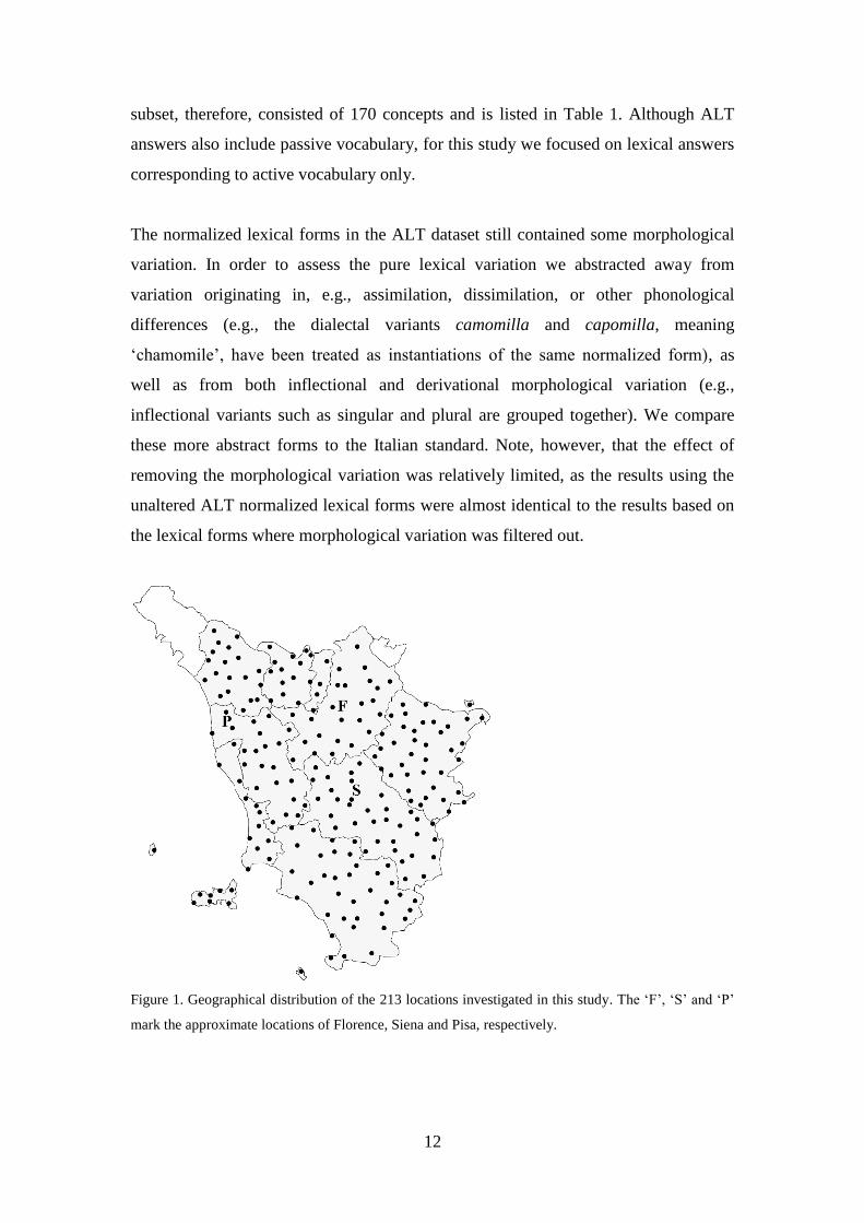
In this study, we focus on Tuscan dialects only, spoken in 213 out of the 224

investigated locations (see Figure 1; Gallo-Italian dialects spoken in Lunigiana and in

small areas of the Apennines were excluded) reducing the number of informants to

2060. We used the normalized lexical answers to a subset of the ALT

onomasiological questions (i.e. those looking for the attested lexicalizations of a given

concept). Normalization was meant to abstract away from phonetic variation and in

particular from productive phonetic processes, without removing morphological

variation or variation caused by unproductive phonetic processes. Out of 460

onomasiological questions, we selected only those which prompted 50 or fewer

distinct normalized lexical answers (the maximum in all onomasiological questions

was 421 unique lexical answers). We used this threshold to exclude questions having

many hapaxes as answers which did not appear to be lexical (a similar approach was

taken by Montemagni, 2007). For example, the question looking for denominations of

‘stupid’ included 372 different normalized answers, 122 of which are hapaxes. These

either represent productive figurative usages (e.g., metaphors such as cetriolo

‘cucumber’ and carciofo ‘artichoke’), productive derivational processes (e.g.,

scemaccio and scemalone from the lexical root scemo ‘stupid’), or multi-word

expressions (e.g., mezzo scemo ‘half stupid’, puro locco ‘pure stupid’ and similar).

From the resulting 195-item subset, we excluded a single adjective and twelve verbs

(as the remaining concepts were nouns) and all twelve multi-word concepts. Our final

12

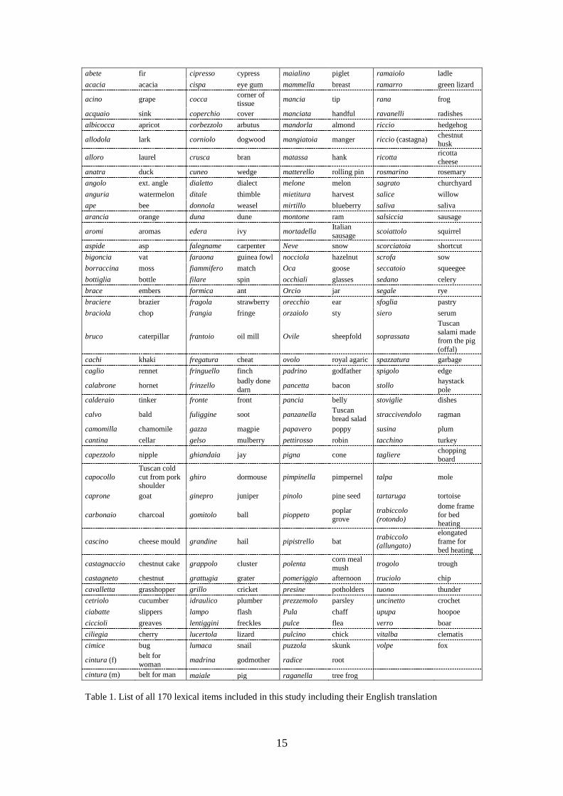
subset, therefore, consisted of 170 concepts and is listed in Table 1. Although ALT

answers also include passive vocabulary, for this study we focused on lexical answers

corresponding to active vocabulary only.

The normalized lexical forms in the ALT dataset still contained some morphological

variation. In order to assess the pure lexical variation we abstracted away from

variation originating in, e.g., assimilation, dissimilation, or other phonological

differences (e.g., the dialectal variants camomilla and capomilla, meaning

‘chamomile’, have been treated as instantiations of the same normalized form), as

well as from both inflectional and derivational morphological variation (e.g.,

inflectional variants such as singular and plural are grouped together). We compare

these more abstract forms to the Italian standard. Note, however, that the effect of

removing the morphological variation was relatively limited, as the results using the

unaltered ALT normalized lexical forms were almost identical to the results based on

the lexical forms where morphological variation was filtered out.

Figure 1. Geographical distribution of the 213 locations investigated in this study. The ‘F’, ‘S’ and ‘P’

mark the approximate locations of Florence, Siena and Pisa, respectively.

13

The list of standard Italian words denoting the 170 concepts was extracted from the

online ALT dialectal resource (ALT-Web; available at

http://serverdbt.ilc.cnr.it/altweb), where it had been created for query purposes, i.e. as

a way for the user to identify the ALT question(s) corresponding to his or her research

interests (see Cucurullo et al., 2006). This list, originally compiled on the basis of

lexicographic evidence, was carefully reviewed by members of the Accademia della

Crusca, the leading institution in the field of research on the Italian language in both

Italy and the world, in order to make sure that it contained undoubtedly standard

Italian forms and not old-fashioned or literary words originating in Tuscan dialects

(see Section 2.2).

In every location multiple speakers were interviewed (see above) and therefore each

normalized answer is anchored to a given location, but also to a specific speaker. As

some speakers provided multiple distinct answers to denote a single concept, the total

number of cases (i.e. concept-speaker-answer combinations) was 384,454.

As Wieling et al. (2011) reported a significant effect of word frequency on dialect

distances from standard Dutch pronunciations (with more frequent words having a

higher distance from standard Dutch, which was interpreted as a higher resistance to

standardization), we obtained the concept frequencies (of the standard Italian lexical

form) by extracting the corresponding frequencies from a large corpus of 8.4 million

Italian unigrams (Brants and Franz, 2009). The corpus-based frequency ranking of

these concepts was then compared to the Grande dizionario italiano dell’uso

(‘Comprehensive Dictionary of Italian Usage’, GRADIT; De Mauro, 2000) which

represents a standard usage-based reference resource for the Italian language

including quantitative information on vocabulary use. In particular, a list of about

7000 high frequency words/concepts highly familiar to native speakers of Italian was

identified in this dictionary, representing the so-called Basic Italian Vocabulary

(BIV). It turned out that 59.4% of the concepts used in our study belonged to the BIV,

whereas the remaining concepts refer to an old-fashioned and traditional world

(19.4%), denote less common plants and animals (14.7%) or refer to kitchen tools

(2.4%). The remaining 4.1% of the concepts represent a miscellaneous class. It is

interesting to note that the classification of concepts with respect to this reference

dictionary and the frequency data obtained from the large web corpus are aligned,

14

with our most frequent concepts being in the BIV and the low frequent concepts

typically corresponding to old-fashioned and traditional notions as well as less

common plants and animals.

3.2.Sociolinguistic data

The speaker information we obtained consisted of the speaker’s year of birth, the

gender of the speaker, the education level of the speaker (ranging from 1: illiterate or

semi-literate to 6: university degree; for this variable about 1.3% of the values were

missing) and the employment history of the speaker (in nine categories: farmer;

craftsman; trader or businessman; executive or auxiliary worker; knowledge worker,

manager or nurse; teacher or freelance worker; common laborer or apprentice; skilled

or qualified worker; or non-professional status such as student, housewife or retired).

Furthermore, we obtained the year of recording for every location and we extracted

demographic information about each of the 213 locations from a website with

statistical information about Italian municipalities (Comuni Italiani, 2011). We

extracted the number of inhabitants (in 1971 or 1981, whichever year was closer to

the year when the interviews for that location were conducted), the average income

(in 2005; which was the oldest information available), and the average age (in 2007;

again the oldest information available) in every location. While the information about

the average income and average age was relatively recent and may not precisely

reflect the situation at the time when the dataset was constructed (between 1974 and

1986), the global pattern will probably be relatively similar.

15

abete fir cipresso cypress maialino piglet ramaiolo ladle

acacia acacia cispa eye gum mammella breast ramarro green lizard

acino grape cocca corner of tissue

mancia tip rana frog

acquaio sink coperchio cover manciata handful ravanelli radishes

albicocca apricot corbezzolo arbutus mandorla almond riccio hedgehog

allodola lark corniolo dogwood mangiatoia manger riccio (castagna) chestnut husk

alloro laurel crusca bran matassa hank ricotta ricotta

cheese

anatra duck cuneo wedge matterello rolling pin rosmarino rosemary

angolo ext. angle dialetto dialect melone melon sagrato churchyard

anguria watermelon ditale thimble mietitura harvest salice willow

ape bee donnola weasel mirtillo blueberry saliva saliva

arancia orange duna dune montone ram salsiccia sausage

aromi aromas edera ivy mortadella Italian

sausage scoiattolo squirrel

aspide asp falegname carpenter Neve snow scorciatoia shortcut

bigoncia vat faraona guinea fowl nocciola hazelnut scrofa sow

borraccina moss fiammifero match Oca goose seccatoio squeegee

bottiglia bottle filare spin occhiali glasses sedano celery

brace embers formica ant Orcio jar segale rye

braciere brazier fragola strawberry orecchio ear sfoglia pastry

braciola chop frangia fringe orzaiolo sty siero serum

bruco caterpillar frantoio oil mill Ovile sheepfold soprassata

Tuscan

salami made from the pig

(offal)

cachi khaki fregatura cheat ovolo royal agaric spazzatura garbage

caglio rennet fringuello finch padrino godfather spigolo edge

calabrone hornet frinzello badly done

darn pancetta bacon stollo

haystack

pole

calderaio tinker fronte front pancia belly stoviglie dishes

calvo bald fuliggine soot panzanella Tuscan bread salad

straccivendolo ragman

camomilla chamomile gazza magpie papavero poppy susina plum

cantina cellar gelso mulberry pettirosso robin tacchino turkey

capezzolo nipple ghiandaia jay pigna cone tagliere chopping board

capocollo

Tuscan cold

cut from pork shoulder

ghiro dormouse pimpinella pimpernel talpa mole

caprone goat ginepro juniper pinolo pine seed tartaruga tortoise

carbonaio charcoal gomitolo ball pioppeto poplar

grove

trabiccolo

(rotondo)

dome frame

for bed heating

cascino cheese mould grandine hail pipistrello bat trabiccolo (allungato)

elongated

frame for

bed heating

castagnaccio chestnut cake grappolo cluster polenta corn meal

mush trogolo trough

castagneto chestnut grattugia grater pomeriggio afternoon truciolo chip

cavalletta grasshopper grillo cricket presine potholders tuono thunder

cetriolo cucumber idraulico plumber prezzemolo parsley uncinetto crochet

ciabatte slippers lampo flash Pula chaff upupa hoopoe

ciccioli greaves lentiggini freckles pulce flea verro boar

ciliegia cherry lucertola lizard pulcino chick vitalba clematis

cimice bug lumaca snail puzzola skunk volpe fox

cintura (f) belt for

woman madrina godmother radice root

cintura (m) belt for man maiale pig raganella tree frog

Table 1. List of all 170 lexical items included in this study including their English translation

16

4. Methods

4.1. Modeling the role of geography: generalized additive modeling

In contrast to a linear regression model in which a single predictor is linear in its

effect on the dependent variable, in a generalized additive model (GAM) the

assumption is relaxed so that the functional relation between a predictor and the

response variable need not be linear. Instead, the GAM provides the user with a

flexible toolkit for smoothing nonlinear relations in any number of dimensions.

Consequently, the GAM is much more flexible than the simple linear regression

model. In a GAM multiple predictors may be combined in a single smooth, yielding

essentially a wiggly surface (when two independent variables are combined) or a

wiggly hypersurface (when three or more independent variables are combined).

A GAM combines a standard linear model with regression coefficients β0 , β1 , . . . , βk

with smooth functions s() for one or more predictors:

Y = β0 + β1 X1 + . . . + βk Xk + s(Xi ) + s(Xj , Xk ) + . . .

A suitable option to smooth a single predictor is to use cubic regression splines. These

fit piecewise cubic polynomials (functions of the form y = a + bx + cx2 + dx

3 ) to

separate intervals of the predictor values. The transitions between the intervals

(located at the knots) are ensured to be smooth as the first and second derivative are

forced to be zero. The number of knots determines how smooth the curve is.

Determining the appropriate amount of smoothing is part of the parameter estimation

process.

To combine predictors which have the same scale (such as longitude and latitude),

thin plate regression splines are a suitable choice. These fit a wiggly regression

surface as a weighted sum of geometrically regular surfaces. When the predictors do

not all have the same scale, tensor products can be used (Wood, 2006: 162). These

define surfaces given marginal basis functions, one for each dimension of the smooth.

The basis functions generally are cubic regression splines (but they can be thin plate

regression splines as well) and the greater the number of knots for the different basis

functions, the more wiggly the fitted regression surface will be. More information

17

about the tensor product bases (which are implemented in the mgcv package for R) is

provided by Wood (2006; Ch. 4). For the interested reader, the appendix shows the

function call used to fit the complete generalized additive mixed-effects regression

model. A more extended introduction about the use of generalized additive modeling

in linguistics can be found in Baayen et al. (2010).

As it turns out, a thin plate regression spline is a highly suitable approach to model the

influence of geography in dialectology, as geographically closer varieties tend to be

linguistically more similar (e.g., see Nerbonne, 2010) and the dialectal landscape is

generally quite smooth (note, however, that the method also can detect steep

transitions between nearby geographical positions). Wieling et al. (2011) also used a

generalized additive model to represent the global effect of geography, as this

measure is more flexible than using e.g., distance from a certain point (Jaeger et al.,

2011). In this study, we will take a more sophisticated approach, allowing the effect of

geography to vary for concept frequency and speaker age. Furthermore, we will use a

generalized additive logistic model, as our dependent variable is binary (in line with

standard sociolinguistic practice using Varbrul; Cedergren and Sankoff, 1974).

Logistic regression does not model the dependent variable directly, but it attempts to

model the probability (in terms of logits) associated with the values of the dependent

variable. A logit is the natural logarithm of the odds of observing a certain value (in

our case, a lexical form different from standard Italian). Consequently, when

interpreting the parameter estimates of our regression model, we should realize that

these need to be interpreted with respect to the logit scale (i.e. the natural logarithm of

the odds of observing a lexical form different from standard Italian). More detailed

information about logistic regression is provided by Agresti (2007)

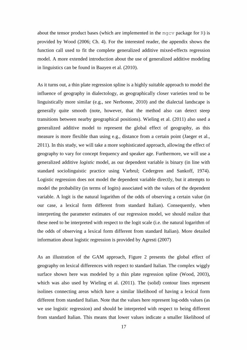
As an illustration of the GAM approach, Figure 2 presents the global effect of

geography on lexical differences with respect to standard Italian. The complex wiggly

surface shown here was modeled by a thin plate regression spline (Wood, 2003),

which was also used by Wieling et al. (2011). The (solid) contour lines represent

isolines connecting areas which have a similar likelihood of having a lexical form

different from standard Italian. Note that the values here represent log-odds values (as

we use logistic regression) and should be interpreted with respect to being different

from standard Italian. This means that lower values indicate a smaller likelihood of

18

being different (intuitively it is therefore easiest to view these values as a distance

measure from standard Italian). Consequently, the value -0.1 indicates that in those

areas the lexical form is more likely to match the Italian standard (the probability is

0.475 that the lexical form is different from the Italian standard form) and the value

0.1 indicates the opposite (the probability is 0.525 that the lexical form is different

from the Italian standard form). Correspondingly, darker shades of gray indicate a

greater likelihood of having lexical forms identical to those in standard Italian, while

lighter shades of gray represent a greater likelihood of having lexical forms different

from those in standard Italian. We can clearly see that locations near Florence

(indicated by the black star) tend to have lexical variants more likely to be identical to

the standard Italian form. This makes sense as Italian originated from the Tuscan

dialect spoken in Florence. The 27.49 estimated degrees of freedom invested in this

general thin plate regression spline were supported by a Chi-square value of 1581 (p <

0.001).

Figure 2. Contour plot for the regression surface of predicting lexical differences from standard Italian

as a function of longitude and latitude obtained with a generalized additive model using a thin plate

regression spline. The (black) contour lines represent isolines, darker shades of gray (lower values)

indicate a smaller likelihood of having a lexical form different from standard Italian, while lighter

shades of gray (higher values) represent locations with a greater likelihood of having a lexical form

different from standard Italian. The black star marks the location of Florence. The white squares

indicate combinations of longitude and latitude for which there is no (nearby) data.

19

As Wieling et al. (2011) found that the effect of word frequency on (Dutch) dialect

distances varied per location, we initially created a three-dimensional smooth

(longitude x latitude x concept frequency), allowing us to assess the concept

frequency-specific geographical pattern of lexical variation with respect to standard

Italian. For example, it might be that the geographical pattern presented in Figure 2,

may hold for concepts having an average frequency, but might be somewhat different

for concepts with a low as opposed to a high frequency. As our initial analyses

revealed that this pattern varied depending on speaker age, we also included the

speaker’s year of birth in the smooth, resulting in a four-dimensional smooth

(longitude x latitude x concept frequency x speaker’s year of birth). We model this

four-dimensional smooth by a tensor product. In the tensor product, we model both

longitude and latitude with a thin plate regression spline (as this is suitable for

combining isotropic predictors and also in line with the approach of Wieling et al.,

2011), while the effect of concept frequency and speaker’s year of birth are modeled

by two separate cubic regression splines.

4.2. Mixed-effects modeling

A generalized additive mixed-effects regression model distinguishes between fixed

and random-effect factors. Fixed-effect factors have a small number of levels

exhausting all possible levels (e.g., gender is either male or female). Random-effect

factors, in contrast, have levels sampled from a much large population of possible

levels. In our study, concepts, speakers and locations are random-effect factors, as we

could have included many other concepts, speakers or locations. By including

random-effect factors, the model can take the systematic variation linked to these

factors into account. For example, some concepts will be more likely to be different

from standard Italian than others (regardless of location) and some locations (e.g.,

near Florence) or speakers will be more likely to use lexical variants similar to

standard Italian (across all concepts). These adjustments to the population intercept

(consequently identified as ‘random intercepts’) can be used to make the regression

formula more precise for every individual location and concept.

20

It is also possible that there is variability in the effect a certain predictor has. For

example, while the general effect of community size might be negative (i.e. larger

communities have lexical variants more likely to match the standard Italian form),

there may be significant variability for the individual concepts. While most concepts

will follow the general pattern, some concepts could even exhibit the opposite pattern

(i.e. being more likely to match the standard Italian form in smaller communities). In

combination with the by-concept random intercepts, these by-concept random slopes

make the regression formula for every individual concept as precise as possible.

Furthermore, taking this variability into account prevents type-I errors in assessing the

significance of the predictors of interest. The significance of random-effect factors in

the model was assessed by the Wald test. More information and an introduction to

mixed-effects regression models is provided by Baayen et al. (2008).

In our analyses, we considered the three aforementioned random-effect factors (i.e.

location, speaker and concept) as well as several other predictors besides the (concept

frequency and speaker age-specific) geographical variation. The additional speaker-

related variables we included were gender, education level and employment history

(coded in 9 binary variables denoting if a speaker has had each specific job or not).

The demographic variables we investigated were community size, average community

age, average community income, and the year of recording.

To reduce the potentially harmful effect of outliers, several numerical predictors were

log-transformed (i.e. community size, average age, average income, education level

and concept frequency). We scaled all numerical predictors by subtracting the mean

and dividing by the standard deviation in order to facilitate the interpretation of the

fitted parameters of the statistical model.

4.3. Combining mixed-effects regression and generalized additive modeling

In contrast to the approach of Wieling et al. (2011), where they first created a separate

generalized additive model (similar to the one illustrated in Figure 2) and used the

fitted values of this model as a predictor in a mixed-effects regression model, we are

able to create a single generalized additive mixed-effects regression model, which

estimates all parameters simultaneously. As the software to construct a generalized

21

additive model is continuously evolving, this approach was not possible previously.

The specification of our generalized additive mixed-effects regression model using

the mgcv package for R is shown in the appendix.

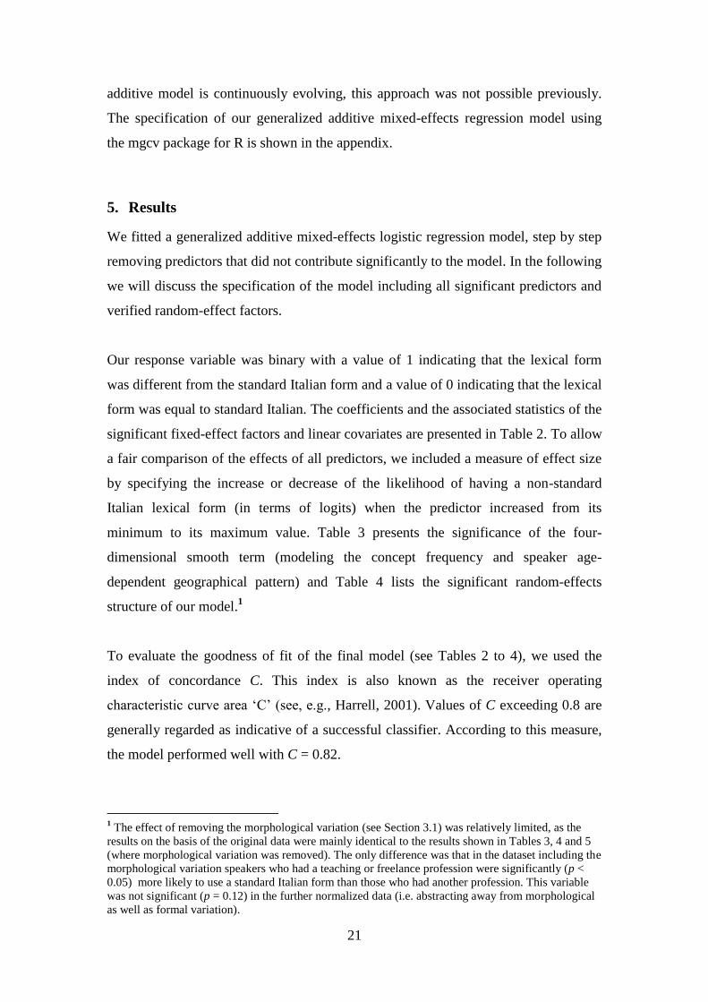
5. Results

We fitted a generalized additive mixed-effects logistic regression model, step by step

removing predictors that did not contribute significantly to the model. In the following

we will discuss the specification of the model including all significant predictors and

verified random-effect factors.

Our response variable was binary with a value of 1 indicating that the lexical form

was different from the standard Italian form and a value of 0 indicating that the lexical

form was equal to standard Italian. The coefficients and the associated statistics of the

significant fixed-effect factors and linear covariates are presented in Table 2. To allow

a fair comparison of the effects of all predictors, we included a measure of effect size

by specifying the increase or decrease of the likelihood of having a non-standard

Italian lexical form (in terms of logits) when the predictor increased from its

minimum to its maximum value. Table 3 presents the significance of the four-

dimensional smooth term (modeling the concept frequency and speaker age-

dependent geographical pattern) and Table 4 lists the significant random-effects

structure of our model.1

To evaluate the goodness of fit of the final model (see Tables 2 to 4), we used the

index of concordance C. This index is also known as the receiver operating

characteristic curve area ‘C’ (see, e.g., Harrell, 2001). Values of C exceeding 0.8 are

generally regarded as indicative of a successful classifier. According to this measure,

the model performed well with C = 0.82.

1 The effect of removing the morphological variation (see Section 3.1) was relatively limited, as the

results on the basis of the original data were mainly identical to the results shown in Tables 3, 4 and 5

(where morphological variation was removed). The only difference was that in the dataset including the

morphological variation speakers who had a teaching or freelance profession were significantly (p <

0.05) more likely to use a standard Italian form than those who had another profession. This variable

was not significant (p = 0.12) in the further normalized data (i.e. abstracting away from morphological

as well as formal variation).

22

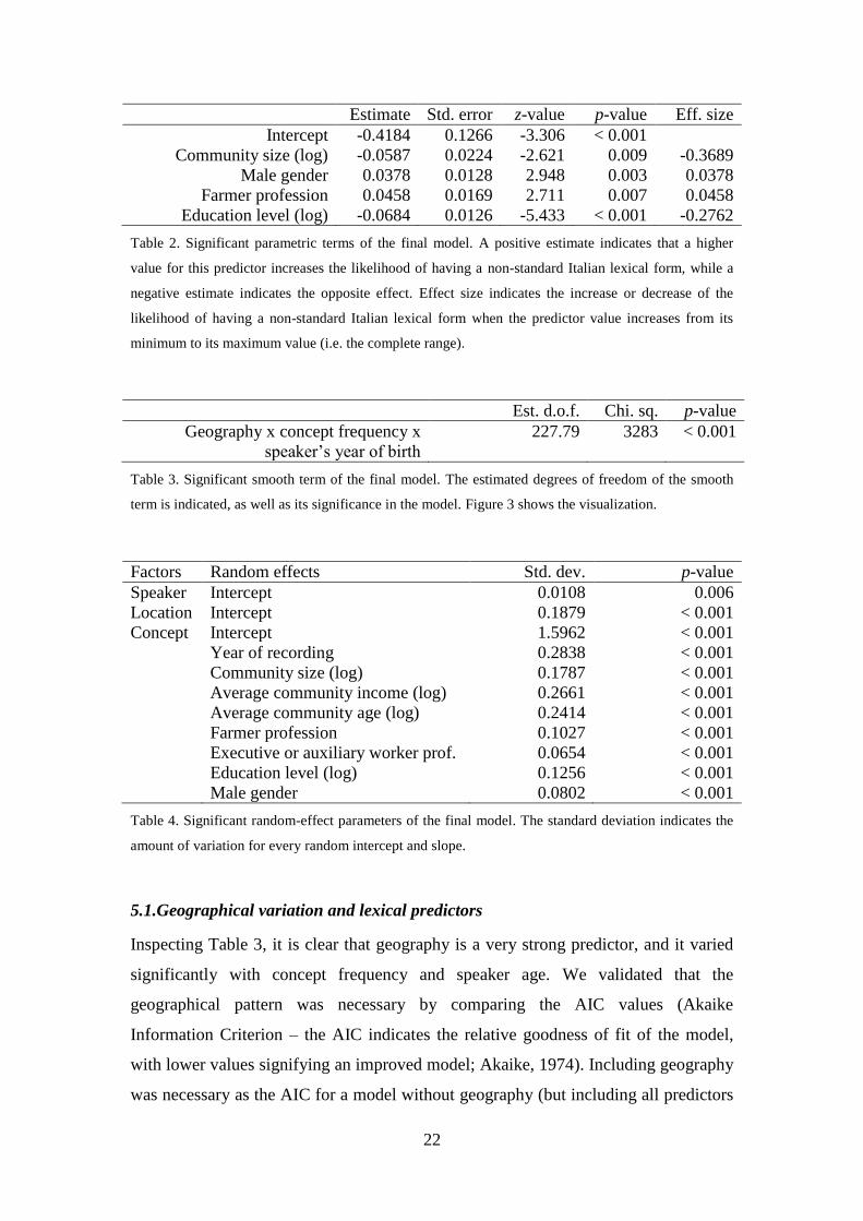
Estimate Std. error z-value p-value Eff. size

Intercept -0.4184 0.1266 -3.306 < 0.001

Community size (log) -0.0587 0.0224 -2.621 0.009 -0.3689

Male gender 0.0378 0.0128 2.948 0.003 0.0378

Farmer profession 0.0458 0.0169 2.711 0.007 0.0458

Education level (log) -0.0684 0.0126 -5.433 < 0.001 -0.2762

Table 2. Significant parametric terms of the final model. A positive estimate indicates that a higher

value for this predictor increases the likelihood of having a non-standard Italian lexical form, while a

negative estimate indicates the opposite effect. Effect size indicates the increase or decrease of the

likelihood of having a non-standard Italian lexical form when the predictor value increases from its

minimum to its maximum value (i.e. the complete range).

Est. d.o.f. Chi. sq. p-value

Geography x concept frequency x

speaker’s year of birth

227.79 3283 < 0.001

Table 3. Significant smooth term of the final model. The estimated degrees of freedom of the smooth

term is indicated, as well as its significance in the model. Figure 3 shows the visualization.

Factors Random effects Std. dev. p-value

Speaker Intercept 0.0108 0.006

Location Intercept 0.1879 < 0.001

Concept Intercept 1.5962 < 0.001

Year of recording 0.2838 < 0.001

Community size (log) 0.1787 < 0.001

Average community income (log) 0.2661 < 0.001

Average community age (log) 0.2414 < 0.001

Farmer profession 0.1027 < 0.001

Executive or auxiliary worker prof. 0.0654 < 0.001

Education level (log) 0.1256 < 0.001

Male gender 0.0802 < 0.001

Table 4. Significant random-effect parameters of the final model. The standard deviation indicates the

amount of variation for every random intercept and slope.

5.1.Geographical variation and lexical predictors

Inspecting Table 3, it is clear that geography is a very strong predictor, and it varied

significantly with concept frequency and speaker age. We validated that the

geographical pattern was necessary by comparing the AIC values (Akaike

Information Criterion – the AIC indicates the relative goodness of fit of the model,

with lower values signifying an improved model; Akaike, 1974). Including geography

was necessary as the AIC for a model without geography (but including all predictors

23

and random-effect factors shown in Table 2 and Table 4) was ...., whereas the AIC for

the model including a simple geographical smooth decreased (i.e. improved) to

392903. Furthermore, varying the geographical effect by speaker age further reduced

the AIC to 392727, while varying it by word frequency resulted in an AIC of 390683.

The best model (with an AIC of 390474) was obtained when the geographical effect

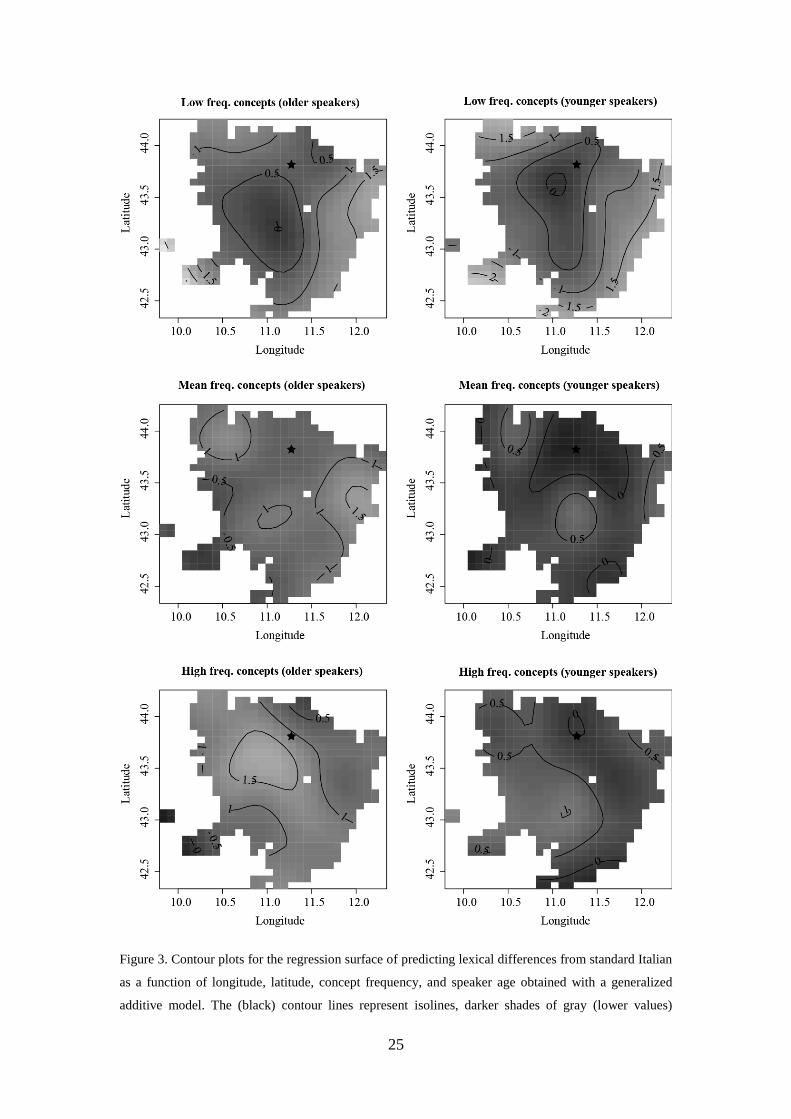
varied depending on word frequency and speaker age. Figure 3 visualizes the

geographical variation related to concept frequency and speaker age. Lighter shades

of gray indicate a greater likelihood of having a lexical form different from standard

Italian.

The three graphs to the left present the geographical patterns for the older speakers,

while those to the right present the geographical patterns for the younger speakers.

When going from the top to bottom, the graphs show the geographical pattern for

increasing concept frequency.

The first observation is that all graphs show the same general trend according to

which speakers from Florence (marked by the star) or the area immediately

surrounding it are more likely to use a standard Italian form than the speakers from

the more peripheral areas. This makes sense as standard Italian originated from

Florence. Note, however, that the likelihood of using a standard Italian form varies

significantly depending on the age of the speakers and the frequency of concepts.

With respect to the age of the speakers, comparing the left and right graphs yields a

straightforward pattern: in all cases, the right graphs are much darker than the left

ones, indicating that the younger speakers are much more likely to use a standard

Italian form. Whereas the right graphs can thus be taken to reflect the standardizing

effect deriving from the increased use of the standard Italian language, the left graphs

are closer to the original pattern of Tuscan dialect variation characterized by a more

limited influence of the standard language. This can be seen as following from the fact

that the older ALT speakers were born between the end of the 19th century and the

beginning of the 20th century. The two series of graphs can thus be seen as separate

windows on different stages of the spreading of standard Italian in a region where the

relationship between dialect and standard language is particularly complex due to the

‘parental’ relationship linking the two.

24

Let us now consider the effect of concept frequency. For the older speakers, we

observe that the lexicalizations of high frequency concepts are less likely to be

identical to standard Italian than those of low frequency concepts (i.e. the graph of the

high frequency concepts is lighter than the graph of the low frequency concepts).

As the standard language also influences dialectal variation in older speakers, the left

graphs in Figure 3 show that this is less effective for the higher frequency words. This

is in line with previous research of Pagel et al. (2007), who found that words denoting

frequently used concepts are less prone to be replaced (possibly because they are

better entrenched in memory and therefore more resistant to lexical replacement).

Furthermore, Wieling et al. (2011) also reported a resistance to standardization for

high frequency words in Dutch dialects.

For the low frequency concepts, older speakers are more likely to use the standard

Italian word. This, in our opinion, should not be seen as the result of standardization

(at least in the majority of cases), but rather of the fact that low frequency concepts in

our dataset typically belong to an obsolete, progressively disappearing rural world

(some examples are bigoncia ‘vat’, seccatoio ‘squeegee’, and stollo ‘haystack pole’).

In this case the specific terms used in central Tuscan dialects to refer to these concepts

are part of the standard Italian vocabulary.

The results recorded for older speakers suggest that the overlap between dialectal and

standard lexical forms in Tuscany is not evenly distributed according to concept

frequency. Overlap with standard Italian was most common for low frequency

concepts, whereas high frequency concepts were more likely to be different from

standard Italian. However, an in-depth explanation of the reasons underlying this state

of affairs would require further analysis and data and therefore goes beyond the scope

of this paper.

25

Figure 3. Contour plots for the regression surface of predicting lexical differences from standard Italian

as a function of longitude, latitude, concept frequency, and speaker age obtained with a generalized

additive model. The (black) contour lines represent isolines, darker shades of gray (lower values)

26

indicate a smaller lexical ‘distance’ from standard Italian (i.e. a smaller likelihood of having a lexical

form different from standard Italian), while lighter shades of gray (higher values) represent locations

with a larger lexical ‘distance’ from standard Italian. The star marks the location of Florence. The left

plots visualize the results for older speakers (two standard deviations below the mean year of birth of

1931, i.e. 1888), while the right plots show those for the younger speakers (two standard deviations

above the mean year of birth of 1931, i.e. 1975). The top row visualizes the contour plots for low

frequency concepts (two standard deviations below the mean), the middle row for concepts having the

mean frequency, and the bottom row for high frequency concepts (two standard deviations above the

mean). The white squares in each graph indicate combinations of longitude and latitude for which there

is no (nearby) data. See the text for interpretation.

For the younger speakers, a slightly different pattern can be observed. While the high

frequency concepts are less likely to be identical to standard Italian than the mean

frequency concepts (due to high frequency concepts being more resistant to change;

Pagel et al., 2007), the low frequency concepts are also less likely to be identical to

standard Italian. A possible explanation for this pattern is that, as previously stated,

the low frequency concepts mostly consist of words from a disappearing rural world.

Younger speakers might lack specific words for denoting these concepts and use more

general terms instead (mismatching with the standard Italian form).

To conclude, we can state that the patterns of lexical choice between standard Italian

and dialect by Tuscan speakers visually represented in Figure 3 do not purely show

the effect of the standard Italian language on the Tuscan varieties, but also the

complex diachronic relationship holding between the Florentine variety and the

standard Italian language.

5.2. Speaker-related predictors

When inspecting Figure 3, it is clear that older speakers were much more likely to use

forms different from standard Italian than younger speakers. This result is not

unexpected as younger speakers tend to converge to standard Italian. In addition, we

found clear support for the significance of gender. Men were much more likely to use

non-standard forms than the standard Italian form. This finding is also not surprising,

given that men generally use a higher frequency of non-standard forms than women

(Cheshire, 2002). Analogous gender differences were reported for Tuscany by

Cravens and Giannelli (1995) for what concerns the spread of intervocalic

27

spirantization of /p/, /t/ and /k/ (i.e. the so-called Tuscan gorgia) as well as by Binazzi

(1996) with respect to the use of dialectal words as opposed to standard Italian in

Florence. Similarly, farmers were also found to be more likely to use non-standard

forms. A reasonable explanation for this is that people living in rural areas (as farmers

tend to do, given the nature of their work) generally favor non-standard forms and are

less exposed to other language varieties (e.g., Chambers and Trudgill, 1998). The final

significant speaker-related variable was education level. Higher educated speakers

used forms more likely to be identical to the Italian standard. Again, this finding is not

unforeseen as higher educated people tend to use more standard forms (e.g., Gorman,

2010).

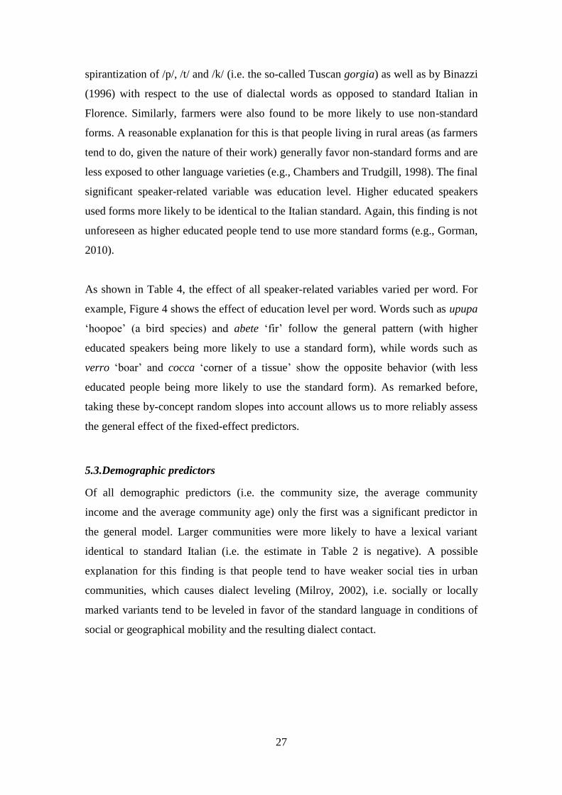
As shown in Table 4, the effect of all speaker-related variables varied per word. For

example, Figure 4 shows the effect of education level per word. Words such as upupa

‘hoopoe’ (a bird species) and abete ‘fir’ follow the general pattern (with higher

educated speakers being more likely to use a standard form), while words such as

verro ‘boar’ and cocca ‘corner of a tissue’ show the opposite behavior (with less

educated people being more likely to use the standard form). As remarked before,

taking these by-concept random slopes into account allows us to more reliably assess

the general effect of the fixed-effect predictors.

5.3.Demographic predictors

Of all demographic predictors (i.e. the community size, the average community

income and the average community age) only the first was a significant predictor in

the general model. Larger communities were more likely to have a lexical variant

identical to standard Italian (i.e. the estimate in Table 2 is negative). A possible

explanation for this finding is that people tend to have weaker social ties in urban

communities, which causes dialect leveling (Milroy, 2002), i.e. socially or locally

marked variants tend to be leveled in favor of the standard language in conditions of

social or geographical mobility and the resulting dialect contact.

28

Figure 4. By-concept random slopes of education level. The concepts are sorted by the value of their

education level coefficient (i.e. the effect of education level of the speakers). The strongly negative

coefficients (bottom left) are associated with concepts that are more likely to be identical to standard

Italian for higher educated speakers, while the positive coefficients (top right) are associated with

concepts that are more likely to be different from standard Italian for higher educated speakers. The

model estimate (see Table 2) is indicated by the dashed line.

The other demographic predictors, average age and average income, were not

significant in the general model. In the study of Wieling et al. (2011) on Dutch

dialects, average age was identified as a significant predictor of pronunciation

distance from standard Dutch, while average income was not. The effect of average

community age may be less powerful in our study, because we also included speaker

age (which is much more suitable to detect the influence of age). In line with Wieling

et al. (2011), the effect of average income pointed to a negative influence (with richer

communities having lexical variants closer to the standard), but not significantly so (p

= 0.5). Also note that year of recording was not significant as a fixed-effect predictor

in the general model, which is likely caused by the relatively short time span (with

respect to lexical change) in which the data was gathered.

29

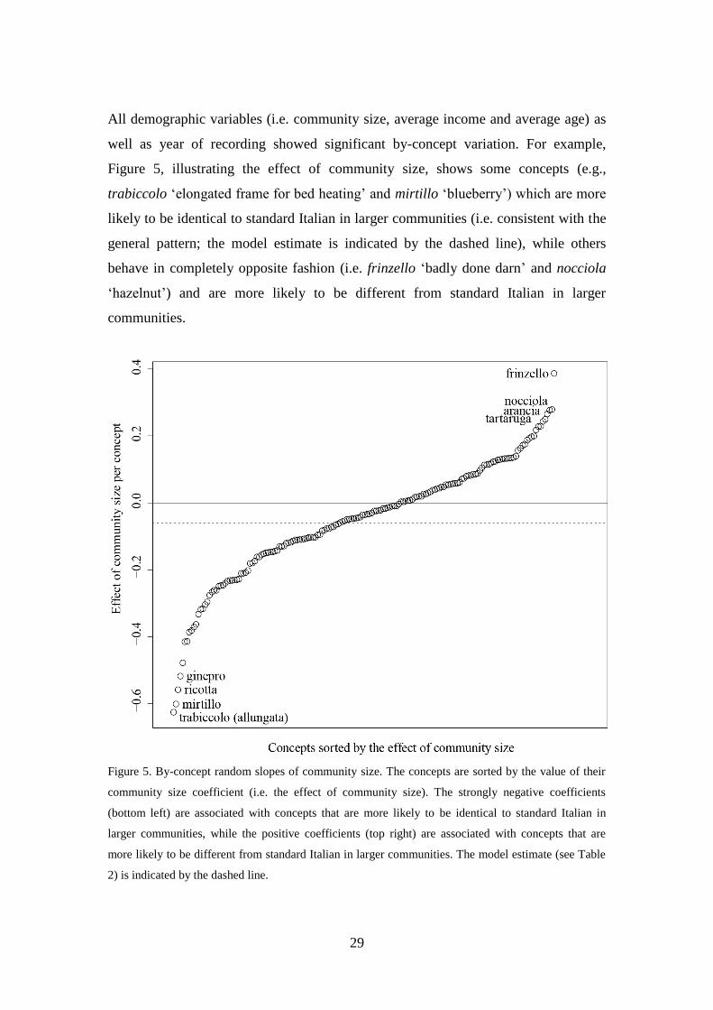
All demographic variables (i.e. community size, average income and average age) as

well as year of recording showed significant by-concept variation. For example,

Figure 5, illustrating the effect of community size, shows some concepts (e.g.,

trabiccolo ‘elongated frame for bed heating’ and mirtillo ‘blueberry’) which are more

likely to be identical to standard Italian in larger communities (i.e. consistent with the

general pattern; the model estimate is indicated by the dashed line), while others

behave in completely opposite fashion (i.e. frinzello ‘badly done darn’ and nocciola

‘hazelnut’) and are more likely to be different from standard Italian in larger

communities.

Figure 5. By-concept random slopes of community size. The concepts are sorted by the value of their

community size coefficient (i.e. the effect of community size). The strongly negative coefficients

(bottom left) are associated with concepts that are more likely to be identical to standard Italian in

larger communities, while the positive coefficients (top right) are associated with concepts that are

more likely to be different from standard Italian in larger communities. The model estimate (see Table

2) is indicated by the dashed line.

30

6. Discussion

In this study we have used a generalized additive model to identify the factors

influencing the lexical choice of Tuscan speakers between dialect and standard Italian

forms. We found clear support for the importance of speaker gender, speaker

education level, speaker profession (i.e. being a farmer), community size, as well as

geography, which varied significantly depending on concept frequency and speaker

age. In addition, we illustrated that the mixed-effects regression approach enabled a

detailed investigation of individual concepts. By simultaneously capturing the

diatopic, diastratic and diachronic (though restricted to only a few generations)

dimensions of variation and by permitting the analysis of individual linguistic

features, we can claim that the proposed method is successful in combining the

dialectometric and sociolinguistic perspectives in the analysis of dialectal lexical data.

The method was tested on a challenging case study focusing on the complex

relationship between Tuscan dialects and standard Italian on the basis of the data

gathered for the Atlante Lessicale Toscano, which turned out to offer an interesting

and unique window into the complex interplay of diachronic and synchronic variation.

The results which have emerged from our analysis of the ALT corpus shed new light

on the typology, impact and role of a wide range of factors underlying the lexical

choices by Tuscan speakers. Previous studies, based both on individual words

(Giacomelli and Poggi Salani, 1984) and on aggregated data (Montemagni, 2008),

provided a flat view according to which Tuscan dialects overlap most closely with

standard Italian in the area around Florence, with expansions in different directions

and in particular towards the southwest. Montemagni’s (2008) aggregate analysis

illustrated that a higher likelihood of using standard Italian was connected with

speaker age and geographical coverage of words. In this study, however, a more

finely articulated picture emerged. For example, we have shown that concept

frequency also plays an important role, with more frequent concepts being more

resistant to change.

On the demographic side, apart from observing that younger speakers were more

likely to use forms identical to standard Italian, we found a significant effect of

speaker gender, profession and education level (with male speakers, lower educated

31

speakers, and farmers using lexical forms more likely to be different from standard

Italian). Our gender-based findings thus provide further evidence supporting the

Labovian Sex/Prestige pattern (Labov, 1966). In addition, we observed that larger

communities are more likely to use standard Italian vocabulary than smaller

communities.

Last but not least, because of the temporal window covered by the ALT dataset it was

possible to keep track of the spreading of standard Italian and its increasing use as a

spoken language. Real standardization effects could only be observed with respect to

younger speakers, whereas older generations turned out to prefer dialectal variants,

especially for high frequency concepts.

A limitation of this study is that it proceeded from dialect atlas data, which inherently

suffers from a sampling bias. Furthermore, to keep the analysis tractable and focus on

purely lexical variation we selected a subset of the data from the dialect atlas. While

still having a relatively large number of items, our dataset only consisted of nouns. As

the influence of word category might also vary geographically (see Wieling et al.,

2011), further research is necessary to see if the results of this study extend to other

word categories.

Another interesting line of research which might be worth pursuing would be to resort

to a more sensitive distance measure with respect to standard Italian such as the

Levenshtein (or edit) distance, rather than the binary lexical difference measure used

in this study. In this case, lexical differences which are closely related (i.e. in the case

of lexicalized analogical formations) can be distinguished from deeper lexical

differences (e.g. due to a different etymon).

Acknowledgements

The research reported in this paper was carried out in the framework of the Short

Term Mobility program of international exchanges funded by CNR (Italy).

32

References

Agresti, A. (2007). An introduction to categorical data analysis. John Wiley & Sons,

Hoboken, NJ, 2nd edition.

Akaike H. (1974). A new look at the statistical identification model. IEEE

Transactions on Automatic Control, 19, 716-723.

Ammon, U. (2004). Standard variety. In U. Ammon, N. Dittmar, K.J. Mattheier and

P. Trudgill (eds.), Sociolinguistics. An International Handbook of the Science of

Language and Society, 2nd edn., vol. 1, Berlin and New York: Mouton de

Gruyter, pp. 273–283.

Baayen, R.H., D.J. Davidson and D.M. Bates (2008). Mixed-effects modeling with

crossed random effects for subjects and items. Journal of Memory and

Language, 59(4), 390-412.

Baayen, R.H, Kuperman, V. and Bertram, R. (2010) Frequency Effects in Compound

Processing. In Sergio Scalise and Irene Vogel (eds). Compounding. Benjamins,

Amsterdam / Philadelphia, 257-270.

Berruto, G. (1989). Main topics and findings in Italian sociolinguistics. International

Journal of the Sociology of Language, 76 [Special issue: Italian sociolinguistics:

Trends and issues], 5–30.

Berruto, G. (2005). Dialect/standard convergence, mixing, and models of language

contact: the case of Italy. In P. Auer, F. Hinskens and P. Kerswill (eds.), Dialect

change. Convergence and divergence in European languages. Cambridge:

Cambridge University Press, pp. 81–97.

Binazzi, N. (1996). Giovani uomini e giovani donne di fronte al lessico della

tradizione: risultati di un’analisi sul campo. In G. Marcato (ed.), Donna e

linguaggio, Atti del Convegno Internazionale di Studi, Sappada/Plodn, 26-30

giugno 1995, Padova, Cleup, pp. 569-579.

Brants, T. and A. Franz (2009). Web 1T 5-gram, 10 European Languages Version 1.

Linguistic Data Consortium, Philadelphia.

Britain, D. (2002). Space and spatial diffusion. In J. Chambers, P. Trudgill and N.

Schilling-Estes (eds.), The Handbook of Variation and Change, Oxford:

Blackwell, pp. 603-637.

Castellani, A. (1982). Quanti erano gli italofoni nel 1861? Studi Linguistici Italiani,

8/1, Roma, Salerno Editrice, pp. 3-26.

33

Cedergren, H.; and Sankoff, D. (1974). Variable rules: Performance as a statistical

reflection of competence. Language, 50, 333-355.

Cerruti, M., (2011). Regional Varieties of Italian in the Linguistic Repertoire.

International Journal of the Sociology of Language, 210, Walter de Gruyter, pp.

9-28.

Comuni Italiani (2011). Informazioni e dati statistici sui comuni in Italia, le province e

le regioni italiane. Sito ufficiale, CAP, numero abitanti, utili link.

http://www.comuni-italiani.it/. Last accessed: 2011-05-23.

Chambers, J.K. and P. Trudgill (1998). Dialectology. Second edition. Cambridge

University Press, Cambridge.

Cheshire, J. (2002). Sex and gender in variationist research. In J.K.Chambers, P.

Trudgill and N. Schilling-Estes (eds.) Handbook of Language Variation and

Change. Blackwell, Oxford, pp. 423-43.

Coltheart, M. (1981). The MRC Psycholinguistic Database. The Quarterly Journal of

Experimental Psychology Section A, 33(4), 497-505.

Coseriu, E. (1980). “Historische Sprache” und “Dialekt”. In J. Göschel, I. Pavle and

K. Kehr (eds.), Dialekt und Dialektologie, Wiesbaden: Steiner, pp. 106 –122.

Cravens, T.D., L. Giannelli (1995). Relative salience of gender and class in a situation

of multiple competing norms. Language Variation and Change, 7, 261-285.

Cucurullo, S., S. Montemagni, M. Paoli, E. Picchi and E. Sassolini (2006). Dialectal

resources on-line: the ALT-Web experience. Proceedings of the 5th

International Conference on Language Resources and Evaluation (LREC-

2006), Genova, Italy, 24-26 May 2006, pp. 1846-1851.

Dal Negro, S. and A. Vietti (2011). Italian and Italo-Romance dialects. International

Journal of the Sociology of Language, 210, 71-92.

De Mauro, T. (1963). Storia linguistica dell'Italia unita. Bari-Roma, Laterza.

De Mauro, T. (2000). Grande dizionario italiano dell'uso. Torino, UTET.

Giacomelli, G. (1975). Dialettologia toscana. Archivio glottologico italiano, 60, 179-

191.

Giacomelli, G. (1978). Come e perchè il questionario. In G. Giacomelli et al. (eds.),

Atlante lessicale toscano - Note al questionario, Firenze, Facoltà di Lettere e

Filosofia, 19-26.

34

Giacomelli, G., L. Agostiniani, P. Bellucci, L. Giannelli, S. Montemagni, A. Nesi, M.

Paoli, E. Picchi and T. Poggi Salani (2000). Atlante Lessicale Toscano. Lexis

Progetti Editoriali, Roma.

Giacomelli, G. and T. Poggi Salani (1984). Parole toscane. Quaderni dell’Atlante

Lessicale Toscano, 2(3), 123-229.

Giannelli, L. (1978). L’indagine come ricerca delle diversità. In G. Giacomelli et al.

(eds.), Atlante lessicale toscano - Note al questionario, Firenze, Facoltà di

Lettere e Filosofia, 35-50.

Goebl, H., (1984). Dialektometrische Studien: Anhand italoromanischer,

rätoromanischer und galloromanischer Sprachmaterialien aus AIS und ALF,

Tübingen, M. Niemeyer.

Goebl, H., (2006). Recent Advances in Salzburg Dialectometry. Literary and

Linguistic Computing, 21(4), 411-435.

Gorman, K. (2010). The consequences of multicollinearity among socioeconomic

predictors of negative concord in Philadelphia. In Lerner, M. (ed.) University of

Pennsylvania Working Papers in Linguistics, volume 16, issue 2, pp. 66–75.

Harrell, F (2001). Regression modeling strategies. Springer, Berlin.

Jaeger, T. F., P. Graff, B. Croft and D. Pontillo (2011). Mixed effect models for

genetic and areal dependencies in linguistic typology: Commentary on

Atkinson. Linguistic Typology, 15(2), 281-319

Johnson, D.E. (2009). Getting off the GoldVarb Standard: Introducing Rbrul for

Mixed-Effects Variable Rule Analysis. Language and Linguistic Compass, 3(1),

359–383.

Labov, W. (1966). The Social Stratification of English in New York City. Center for

Applied Linguistics, Washington, DC.

Labov, W. (l972). Sociolinguistic Patterns. University of Pennsylvania Press,

Philadelphia, PA.

Lepschy, G. (2002). Mother Tongues & other Reflections on the Italian Language.

University of Toronto Press, Toronto.

Loporcaro, M. (2009). Profilo linguistico dei dialetti italiani, Roma-Bari, Laterza.

Maiden, M. (1995). A Linguistic History of Italian. Longman, London.

Maiden, M. and M. Parry (1997). The Dialects of Italy. Routledge, London.

Migliorini, B. and T.G. Griffith (1984). The Italian language. Faber and Faber,

London.

35

Milroy, L. (2002). Social Networks. In J. Chambers, P. Trudgill and N. Schilling-

Estes (eds.), The Handbook of Language Variation and Change. Blackwell

Publishing Ltd., pp. 549-572.

Montemagni, S., M. Wieling, B. de Jonge and J. Nerbonne (2012). Patterns of

Language Variation and Underlying Linguistic Features: A New Dialectometric

Approach. In Bianchi, P., De Blasi, N., De Caprio, C. and Montuori, F. (eds), La

variazione nell'italiano e nella sua storia. Varietà e varianti linguistiche e

testuali. Atti dell'XI Congresso SILFI (Società Internazionale di Linguistica e

Filologia Italiana). Firenze: Franco Cesati Editore, vol. II, pp. 879-889.

Montemagni, S., M. Wieling, B. de Jonge and J. Nerbonne (2013). Synchronic

Patterns of Tuscan Phonetic Variation and Diachronic Change: Evidence from a

Dialectometric Study. Literary and Linguistic Computing, 28(1), 157-172.

Montemagni, S. (2007). Patterns of phonetic variation in Tuscany: using

dialectometric techniques on multi-level representations of dialectal data. In P.

Osenova et al. (eds.), Proceedings of the Workshop on Computational

Phonology at RANLP-2007, pp. 49-60.

Montemagni, S. (2008). Analisi linguistico-computazionali del corpus dialettale

dell'Atlante Lessicale Toscano. Primi risultati sul rapporto toscano-italiano. In

A. Nesi and N. Maraschio (eds.), Discorsi di lingua e letteratura italiana per

Teresa Poggi Salani (Strumenti di filologia e critica, vol. 3), Pisa, Pacini, pp.

247-260.

Nerbonne, J., W. Heeringa, E. van den Hout, P. van de Kooi, S. Otten, W. van de Vis

(1996). Phonetic Distance between Dutch Dialects. In G. Durieux, W.

Daelemans, S. Gillis (eds.), Proceedings of the Sixth CLIN Meeting (Antwerp,

Centre for Dutch Language and Speech, UIA), pp. 185-202.

Nerbonne, J. and P. Kleiweg (2007). Toward a dialectological yardstick. Journal of

Quantitative Linguistics, 14(2), 148-167.

Nerbonne, J., (2003). Linguistic Variation and Computation. In Proceedings of the

10th Meeting of the European Chapter of the Association for Computational

Linguistics, 15-17 April 2003, Budapest, Hungary, pp. 3-10

Nerbonne, J. (2009). Data-driven dialectology. Language and Linguistics Compass,

3(1):, 175-198.

Nerbonne, J. (2010). Measuring the diffusion of linguistic change. Philosophical

Transactions of the Royal Society B: Biological Sciences, 365, 3821-3828.

36

Pagel, M., Q. Atkinson and A. Meade (2007). Frequency of word-use predicts rates of

lexical evolution throughout Indo-European history. Nature, 449, 717-720.

Poggi Salani, T. (1978). Dialetto e lingua a confronto. In G. Giacomelli et al., Atlante

lessicale toscano - Note al questionario, Firenze, Facoltà di Lettere e Filosofia,

pp. 51-65.

Seguy, J. (1973). La dialectométrie dans l’atlas linguistique de gascogne. Revue de

Linguistique Romane, 37(145), 1–24.

Tagliamonte, S.A. and R.H. Baayen (2012). Models, forests, and trees of York

English: Was/were variation as a case study for statistical practice. Language

Variation and Change, 24(2), 135-178.

Valls, E., M. Wieling and J. Nerbonne (2013). Linguistic Advergence and Divergence

in Northwestern Catalan: A Dialectometric Investigation of Dialect Leveling

and Border Effects. Literary and Linguistic Computing, 28(1), 119-146.

Wattenmaker, W.D. and E.J. Shoben (1987). Context and the recallability of concrete

and abstract sentences. Journal of Experimental Psychology: Learning,

Memory, and Cognition, 13(1), 140-150.

Wieling, M., J. Nerbonne and R.H. Baayen (2011). Quantitative Social Dialectology:

Explaining Linguistic Variation Socially and Geographically. PLOS ONE, 6(9),

e23613.

Wieling, M. and J. Nerbonne (2010). Hierarchical spectral partitioning of bipartite

graphs to cluster dialects and identify distinguishing features. Proceedings of

the 2010 Workshop on Graph-based Methods for Natural Language Processing,

ACL, Uppsala, Sweden, 16 July 2010, pp. 33-41.

Wieling, M. and J. Nerbonne (2011). Bipartite spectral graph partitioning for

clustering dialect varieties and detecting their linguistic features. Computer

Speech and Language, 25(3), pp. 700-715.

Wieling, M., R.G. Shackleton and J. Nerbonne (2013). Analyzing phonetic variation

in the traditional English dialects: Simultaneously clustering dialects and

phonetic features. Literary and Linguistic Computing, 28(1), 31-41.

Wieling, M. (2012). A Quantitative Approach to Social and Geographical Dialect

Variation. PhD Thesis, University of Groningen.

Wood, S. (2003). Thin plate regression splines. Journal of the Royal Statistical

Society: Series B (Statistical Methodology), 65(1), 95-114.

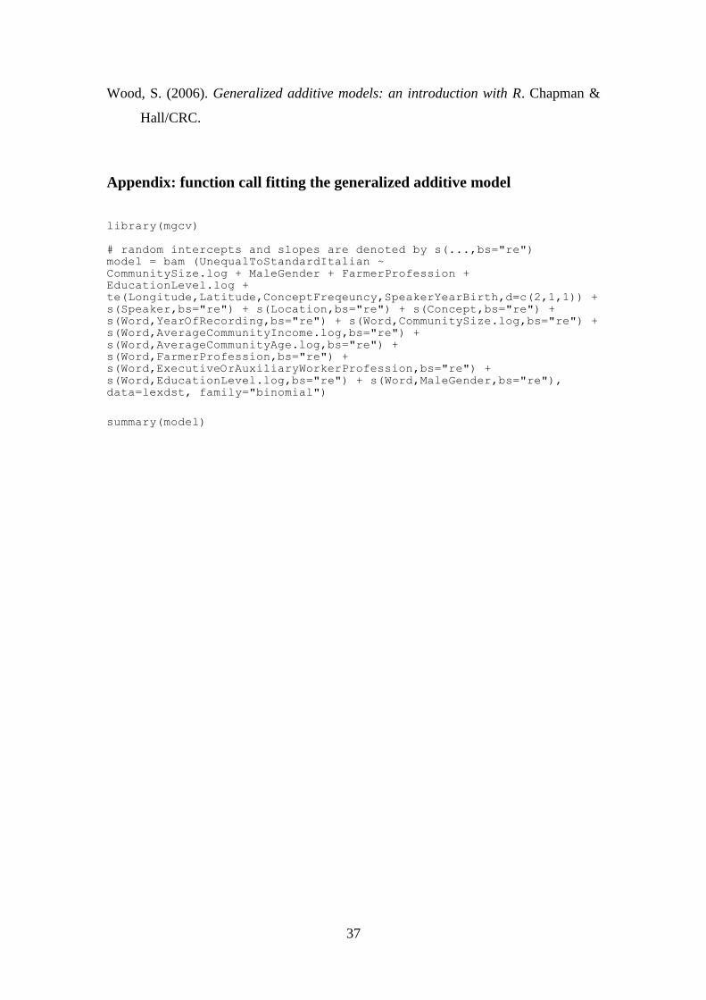
37

Wood, S. (2006). Generalized additive models: an introduction with R. Chapman &

Hall/CRC.

Appendix: function call fitting the generalized additive model

library(mgcv)

# random intercepts and slopes are denoted by s(...,bs="re")

model = bam (UnequalToStandardItalian ~

CommunitySize.log + MaleGender + FarmerProfession +

EducationLevel.log +

te(Longitude,Latitude,ConceptFreqeuncy,SpeakerYearBirth,d=c(2,1,1)) +

s(Speaker,bs="re") + s(Location,bs="re") + s(Concept,bs="re") +

s(Word,YearOfRecording,bs="re") + s(Word,CommunitySize.log,bs="re") +

s(Word,AverageCommunityIncome.log,bs="re") +

s(Word,AverageCommunityAge.log,bs="re") +

s(Word,FarmerProfession,bs="re") +

s(Word,ExecutiveOrAuxiliaryWorkerProfession,bs="re") +

s(Word,EducationLevel.log,bs="re") + s(Word,MaleGender,bs="re"),

data=lexdst, family="binomial")

summary(model)