1

April 2007

Liberalising Border Trade: Implications for Domestic Agricultural Markets of India Rajesh Chadha, Devender Pratap and Anjali Tandon

Paper prepared for Tenth Annual Conference on Global Economic Analysis Purdue University West Lafayette, IN, U.S.A. June 7-9, 2007

2

Liberalising Border Trade: Implications for Domestic Agricultural Markets of India1

Rajesh Chadha, Devender Pratap and Anjali Tandon2

I. Introduction

India has completed 15 years of its economic reform process in July 2006. It has also been an

active Member of the WTO and has participated in the global trade liberalisation undertaken since 1994 under the Uruguay Round Agreement. Agriculture has special importance for

India since it is a crucial sector of the economy. More than 55 per cent of working population is engaged in agriculture, which accounts for less than 20 per cent of India’s GDP.

A large majority of the farmers are small and poor. Thus any attempt that impacts Indian agriculture has to meet the test of maximising gains to the poorest of the farmers while

minimising any policy-induced losses for them.

Agricultural trade in the country, both domestic and international, had been highly regulated until the early 1990s. There has been gradual opening up of both internal and external trade in

agricultural goods since 1991. While domestic trade has taken much longer time and still continues to remain regulated in various ways, international trade in agricultural goods has

seen relatively fast liberalisation.

The interaction of the domestic and border trade policies became quite evident during the late 1990s. During 1990s, Indians witnessed the minimum support prices (MSPs) 3 of rice and

wheat growing rapidly and out of concert with domestic markets. One major reason was that the cost of production became a full-cost measure since 1997-98. 4 The second factor related

to the changes in India’s rice export policies during 1995 and 1996. In the case of rice, the 1 This paper is based on a study of Indian agricultural markets conducted at the National Council of Applied Economic Research, New Delhi and funded jointly by the British High Commission, New Delhi and Australian Centre for International Agricultural Research, Canberra. Rajesh Chadha: Senior Fellow, NCAER, New Delhi - rchadha@ncaer.org Devender Pratap: Associate Fellow, NCAER, New Delhi - dpratap@ncaer.org Anjali Tandon: Research Analyst, NCAER, New Delhi - atandon@ncaer.org 2 Authors are extremely thankful to Professor Ramesh Chand, ICAR National Professor, National Centre for Agricultural Economics and Policy Research (NCAP), New Delhi, Professor Arvind Panagariya, Jagdish Bhagwati Professor of Indian Political Economy, Columbia University and Professor Thomas W. Hertel, Executive Director, Center for Global Trade Analysis for providing very useful comments on earlier drafts of this paper.

3 The minimum support prices (MSP) are announced by the government with a view to ensuring remunerative prices to the farmers for their produce on the basis of the Commission for Agricultural Costs and Prices (CACP) recommendations. Farmers perceive MSP as a guarantee price for their produce from the Government. These prices are announced by the Government at the commencement of the season to enable them to pursue their efforts with the assurance that the prices would not be allowed to fall below the level fixed by the government.

4 The full-cost measure of the cost of cultivation includes imputed value of family labour in addition to all the paid-out costs of cultivation comprising a) hired human , animal and machine labour; b) maintenance expenses on owned animals and machinery; c) costs of material inputs including seeds, fertilisers, manure, pesticides and irrigation; d) depreciation on implements and farm buildings; e) land revenue; f) rent paid out for leased land; and g) imputed value of owned land,

3

removal of export restraints led to higher market prices , which consequently resulted in

pressure to keep MSP high even as the world prices declined. In the case of wheat, re-imposition of export restraints led to lower market prices and the Government could not resist

continuing with high MSP. The main reason for raising MSP was to integrate domestic prices with international prices which were on the higher side during 1995-1998. This was done on

recommendations by some of the economists who stressed upon the fact that India had negative Aggregate Measure of Support (AMS) (Chand, 2003 and 2005). Global price trends

are based on two alternative forces: i.e., subsidies and tariff policies adopted by major producing countries and productivity and marketing efficiency gains reaped by many parts of

the world. India has not been reaping such benefits (Landes and Gulati, 2004).

The post economic reform period since 1991 witnessed improvement in domestic terms of trade of agriculture vis-à-vis manufacturing industry mainly due to initial rapid lowering of

tariff protection enjoyed by the manufactured goods. However, major beneficiaries have been wheat and rice through rapid increase in their minimum support prices. Since the mid-

nineties,,, this, however, has not led to corresponding growth of their output because the major wheat and rice growing regions have already exhausted their production potential and

the price support was not equally available in the regions with low yield and high potential for growth.

Even though there was a difference between MSPs and procurement prices5 initially, since

1991-92, only the former were announced. The calculation method of MSPs has kept changing over time. The Commission for Agricultural Costs and Prices (CACP) recommends

the levels at which MSP should be fixed. However, MSP fixatio n is influenced by political considerations. Also, the India n Government’s price stabilisation program dampened

seasonal price rise , which discouraged farmers and traders from storing grains after harvest until they could get higher prices.

Agricultural commodities are sold by the farmers through four marketing channels,6 viz. a)

direct to consumers; b) through wholesalers and retailers; through public agencies; and d) through processors. The government intervenes in agricultural trade through purchase of

agricultural commodities under the MSP programme, procurement of foodgrains, monopoly purchase, open market purchases of commodities, etc. In the case of foodgrains (particularly

rice and wheat), the government purchase agency (Food Corporation of India) is an important market functionary for cereals. State agencies including National Cooperative Marketing

5 Procurement prices were announced before the harvest season, along with the MSP, during 1970-71 and 1990-91. The procurement prices were higher than the corresponding MSPs but lower than the market prices . The public agencies would buy some desired volumes of commodities at procurement prices though the price guarantees remained at the MSPs. The public agencies were and are obliged to buy all that the farmers have to offer at the MSPs subject to the commod ities meeting some “fair average quality”. 6 Acharya (2004).

4

Federation of India (NAFED)7, Cotton Corporation of India (CCI) and Jute Corporation of

India (JCI) enter into open market procurement of various agricultural commodities. The government also puts compulsory levy procurement of a declared proportion on the output of

some of the agro-processed commodities on the processing factories (for example rice and sugar) to be procured at less than the market prices from the processing mills for distribution

to the relatively poor consumers. These parastatal organisations have played active role in India’s agricultural marketing. The share of private trade remains fairy high in proportion

compared with the corresponding share handled by the parastatals.

The conventional reasons for maintaining the food-marketing parastatals do not actually hold any more. The costs of price stabilisation through these parastatal agencies are high and

increasing as compared with private sector’s operations. Some special interest and rent-seeking groups are the dictators and protectors of this system. Liberalisation of foodgrain

markets appears to have beneficial effects through freeing the locked resources of the Government for better usage through investments and implementing poverty alleviation

schemes like National Food for Work Programme, National Rural Employment Guarantee Scheme, Indira Housing Schemes and National Social Assistance Programme.

It has become clear that many of the interventions have outlived their usefulness and, in many

cases, have not only become a drag on the growth and viability of the agriculture sector, but on the entire economy. A particularly dramatic illustration of this has been the large and

wasteful build up of grains (rice and wheat) stocks during 1999-2002 resulting from high government procurement prices in practice available only to a minority of farmers in select

states. Such procurement was biased in favour of 5 states, in which most of the procurement is concentrated.

It is in India’s interest to minimise divergences between global and domestic prices and

maximise efficiency gains from aligning domestic with foreign prices. In this context, the interface between domestic market reforms and reforms in international trade are particularly

important, and have probably received less explicit recognition than is necessary in much of the existing work on agricultural market reforms. This link, however, is critical to the future

development of India n agriculture.

The degree to which global price changes will influence domestic producer and consumer prices depends not only on government procurement price changes but also on the nature of

the marketing chain and market structure. Typically, empirical analysis of the effects of the international trade regime (affecting border prices) assumes full pass through, which is

unlikely to be the case in reality. Unless domestic markets are perfectly competitive , the degree of ‘pass through’ of border price changes to domestic prices will be muted, and direct

government interventions – such as government procurement policies and operations of state 7 NAFED deals in marketing of oilseeds. Pulses, horticulture, spices, etc. (http://www.nafed-india.com)

5

trading enterprises (STEs) more generally – will further modify the pass through process. On

the other hand, the impact of various government interventions in domestic markets, and outcomes of domestic market reforms also interact with changes to the international trade

regime that operate at the border.

The marketing of Indian agricultural commodities within the countr y suffers from the excessive government interventions. There is an obvious need to liberalise domestic

agricultural markets from the existing, and even non-existing, regulated physical markets in favour of private markets, forward markets, and contract farming. The operations of the

government machinery for public procurement and distribution also suffer from various weaknesses vis-à-vis advances already made in border liberalisation of agricultural trade.

The progressive removal of restrictions8 on internal movement of agricultural commodities

has gradually increased the degree of domestic market integration. The government has clearly stated its commitment to greater market integration. The Inter-Ministerial Task Force

on Agricultural Marketing Reforms (2002) recommended that the Agricultural Produce Market Committee (APMC) Acts need to be amended by the State Governments to

specifically provide for: a) promotion of agricultural markets in private / cooperative sector 9; b) encouragement of direct marketing; c) enabling contract farming arrangements; d)

rationalisation of market fee10; e) amendment of the Essential Commodities Act (1955) 11; f) pledging of financing and marketing credit; and g) enabling negotiable warehousing receipt

system.

The Central Government drafted the State Agricultural Produce Marketing (Development and Regulation) Act, 2003, also known as Model Act (2003), and recommended its adoption to

the states at the National Conference of State Ministers held on January 7, 2004 in New Delhi and on November 19, 2004 in Bangalore. It states that Government regulated wholesale

market monopoly has prevented development of a competitive marketing system in the country, failing to provide help to the farmers in direct marketing, organizing retailing, a

smooth raw material supply to agro-processing industries and adoption of innovative marketing system and technologies. Exporters, processors, and retail chain operators have not

been able to get specific quality and quantity of produce for their business because direct marketing has not been allowed. The processor has not been free to buy the produce at the 8 The restrictions generally take legislative forms. These include, for instance, Essential Commodities Act, 1955, Food Grains (Procurement and Licensing) Order, 1952, Sugar Control Order, 1956 and Pulses, edible oilseeds and edible oils (Storage) Control Order, 1977. These Acts, in general, control production, supply, storage and movement of agricultural commodities. 9 In 2003, the government of Karnataka state taken initiative for collaborating with National Dairy Development Board (NDDB), a co -operative body, for establishment of an “Integrated Produce Market” for marketing of fruits, vegetables and flowers in the state. 10 The market fee includes the charges levied by the regulated markets for providing various amenities in the market yard. The rate of this fee varies from 0.5 to 2.0 per cent of the value of the output transacted. 11 The Essential Commodities Act was designed to minimise the practice of ‘hoarding of agricultural commodities” to get advantage of artificial scarcity resulting in higher market prices.

6

processing plant or at the warehouse but has had to buy only from the market yard. Finally,

while a certain percentage of income of APMCs (which varies from state to state) goes to the State Marketing Board to be used for development of markets etc., there have been cases of

funds being transferred for other purposes by State Governments.

According to information compiled by Directorate of Marketing and Inspection (DMI)12 on 31st January 2006, some states such as Andhra Pradesh, Himachal Pradesh, Madhya Pradesh,

Maharashtra, Punjab and Rajasthan have already made amendments to their Agricultural Produce Market Acts in order to incorporate suggestions made by the Model Act. For

example , Andhra Pradesh allows setting up of private markets/direct marketing under the proposed Rule 53-A. It also allows contract farming based on some conditions , such as the

buyer being registered in the notified area of the market committee wherein the land of the contract farming producer is situated. In Maharashtra a license is granted to any person for

establishing a private market for certain specified activities and direct marketing is allowed, as per a new chapter 1-B, section 5-D. But there is still no institutional support to enable

contract farming through registration of the sponsoring company, recording of the contract farming agreement in Maharashtra. The Model Act would be actually successful only when

all the states amend their Acts, so that benefits are available for all farmers.

A total withdrawal of the state from agricultural price setting is improbable in the foreseeable future. Despite the considerable momentum of reform, it is unlikely that prices of staple

grains – core ‘political’ prices – will be allowed to fluctuate freely in line with domestic or international market trends. The trade reforms at the border that removed some of the

restrictions on international trade in rice led to rice exports (at the low quality end) to the global market. However, this did not mean an end to the government interventions in rice

markets. When world rice prices declined, domestic price set by the government mechanisms, the MSPs in particular, were used to prevent domestic prices from adjusting or reflecting

world market trends, increasing subsidy costs (Landes and Gulati, 2004). This is also likely to be true of other agricultural commodities, though perhaps to a lesser degree. Nevertheless, a

greater reliance on market instruments to achieve price stability and food security ought to be on the agenda.

What we see already, and what we may see even more in the future, are agricultural markets

where various types of state trading enterprises will co-exist with groups of other pr ivate market players. Empirical observations of deregulated agricultural commodity markets in

both developing and developed countries suggests that markets are likely to be imperfectly competitive with a relatively small number of large traders, each of whom is able to exert

some market power. The analysis of the effects of STEs in agricultural product markets is made difficult for two reasons. The first is that STEs are by no means homogeneous entities.

12 Please refer to AGMARKNET website at http://agmarknet.nic.in/amrscheme/compprovimain.htm

7

As reported by the WTO Working Group on STEs (WTO, 1995), the Working Group was

able to identify seven types of STE which collectively pursue nine different objectives and which have varying degrees of government involvement. The second difficulty is that the

benchmark or contrary facts against which to compare the market effects of STEs are not known with any precision. The empirical evidence from commodity markets in which STEs

do not exist, or in which they are a minor component, is that such markets are more accurately described as oligopolistic and/or oligopsonistic. Yet many of the early results on

market distortions created by STEs in theoretical analysis assumed perfect competition. More recent work has paid more attention to alternative benchmarks in imperfect

competition.13

II. Trade Policy

External trade in agriculture was heavily controlled by the government parastatals through a web of quantitative restrictions, licensing and canalisation of exports and imports by

parastatals. Agriculture was not covered in the trade liberalisation measures taken during 1991 and 1992, apart from relaxation of some export controls.

The pace of the reform of external policies in agriculture picked up in 1993-94. Since then

significant measures have been taken to liberalise agricultural trade policy. Tariffs have been reduced, quantitative restrictions on agricultural trade have been removed, and agricultural

trade has been decanalised with the exception of mainly some edible oils and some cereals among agricultural products. However, the tariff regime continues to be complex.

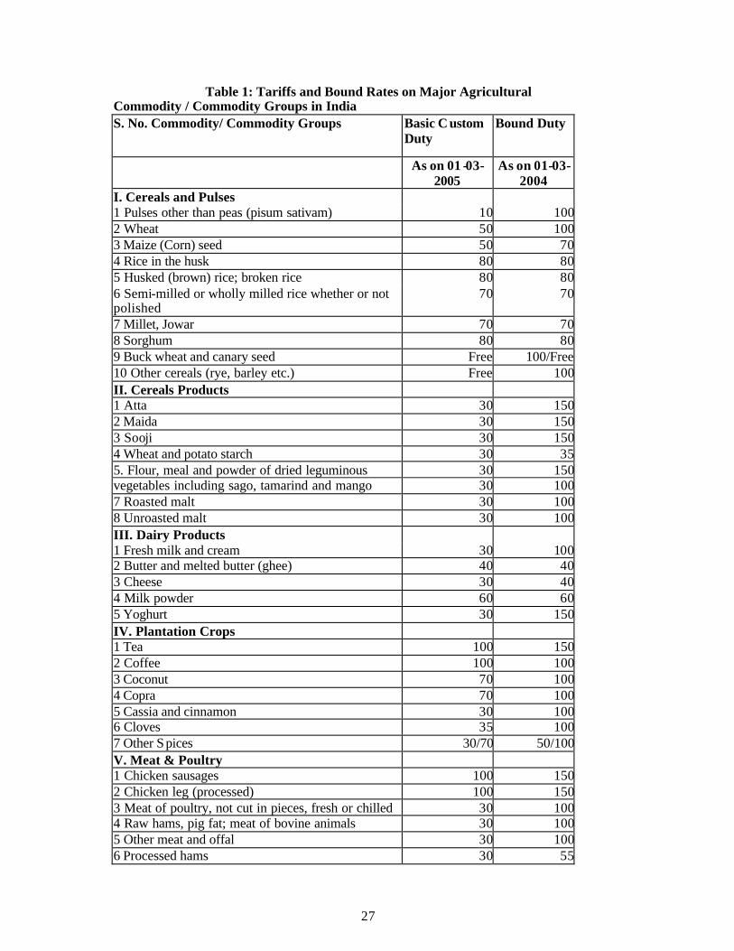
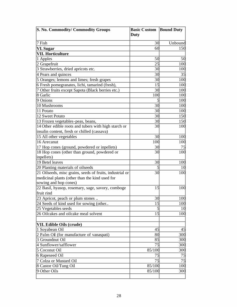
At present, India has tariff bindings on 100 per cent of agricultural products based on the

WTO definition of agriculture. Bindings were not made in the case of fish and crustacean products. All tariff rates have been bound with tariff bindings ranging from 100-104 per cent

for raw products including cereals, vegetables and fruits, oilseeds, pulses; 150 per cent for semi-processed products like tea, processed chicken, wheat flour; and 300 per cent for

vegetable oils and fats with some exceptions (Table 1). In fact, until 1998-99 there was no duty on import of cereals but their imports were canalised. Duty on wheat was introduced in

1999-2000 and on rice in 2000-01.

India commenced the process of removing its Quantitative Restrictions (QRs) on consumer goods on April 1, 2001. Some of the bindings for a number of cereals have been renegotiated.

The final average bound tariff as per India's commitments is expected to be 115.7 per cent. The average bound tariff is much higher than the actually applied tariff in average on the

MFN basis. The simple average applied tariff on India's imports of agricultural products

13 See Lavoie (2003) by McCorriston and MacLaren (2005a and 2005b) and by Veeman et al (1999)

8

(WTO definition) declined after the initiation of the reforms in 1991 to 35 per cent in 1997-

98 but increased to 41 per cent in 2001-02 (Table 2).

Tariffs for some agricultural and allied products have increased since 2001 as a result of removal of quantitative restrictions on imports. India was obliged to remove all quantitative

restrictions on imports by the decision of the WTO dispute pane l as it was no longer suffering from balance of payments problems (WT/DS90/AB/R). According to WTO (2002), tariffs

were increased to 37.5 per cent for the cases in which quantitative restrictions were removed. The increases have occurred mainly in case of live animals, foodgrains, oilseeds and fats.

According to the Foreign Trade Policy (FTP: 2004-2009), exports and imports shall be free

from restrictions , except in cases where they are regulated by the provisions of the Policy or any other law in force at the time.14 The item-wise export and import policy shall be

amended from time to time, as specified in Indian Trade Classification Harmonised System (ITC - HS) published and notified by Director General of Foreign Trade (DGFT). Any goods,

the export and import of which is governed through exclusive or special privileges granted to the STEs, may be imported or exported by the STEs as specified in the ITC - HS codes

subject to the conditions specified therein. The DGFT may, however, grant a license / certificate / permission / authorisation to any other person to import or export any of these

goods.

With respect to goods , the import of which is governed through exclusive or special privileges granted to STEs, the FTP: 2004-2009 states the STEs shall make any such

purchases or sales involving imports or exports solely in accordance with commercial considerations, including price, quality, availability, marketability, transportation, and other

conditions of purchase and sale. The enterprises shall act in a non-discriminatory manner and shall afford the enterprises of other countries adequate opportunity, in accordance with

customary business practices, to compete for participation in such purchases or sales. Imports of all cereals, except barley, are subject to STE controls.

III. Multilateral Trade Negotiations in Agriculture

The pace and progress of the Uruguay Round of trade negotiations, which was launched in

September 1986 at Punta del Este, Uruguay, was largely determined by the negotiations pertaining to agriculture. The conclusion of the Round was delayed due to participants’

inability to reach an agreement over agricultural negotiations. The Final Act was signed in April 1994 at Marrakesh, Morocco and became effective on January 1, 1995. The provisions

relating to agriculture are contained in the Agreement on Agriculture (URAA), also known as 14 Foreign Trade Policy is announced by the Ministry of Commerce and Industry (Department of Commerce), Government of India. The latest version is available at http://dgftcom.nic.in/exim/2000/policy/plcontents06.htm

9

the Uruguay Round Agriculture Agreement (URAA), and the Agreement on the Application

of Sanitary and Phytosanitary Measures, which form part of the WTO Agreement. The detailed commitments on agriculture of the WTO members are contained in the agricultural

component of the country schedules, which form part of the overall agreement reached in the Round and form an important adjunct of GATT (1994). The stipulated reduction

commitments, method of calculation and other details are specified in a separate Modalities document appended to the WTO Agreement. The URAA consists of total of 21 articles and is

structured around three major areas: market access, domestic support, and export competition. Apart from establishing rules and rates of reduction, the URAA also established

the institutional mechanism in the form of the Committee on Agriculture to review the implementation of the Agreement on Agriculture (Chadha et al, 2005).

A. An Assessment of the Agreement on Agriculture

Implementation of the UR over the period of 1995 and 2006 has led to little reduction in

agricultural protection. Although the UR commitments have not resulted in large reductions in agricultural protection, the UR made a breakthrough in establishing a framework for more

meaningful reductions in the Doha Round and subsequent WTO discussions.

Some specific points of URAA that came under criticism and are disadvantageous to developing countries like India may be summarised as follows:

• The selection of the base year, for the conversion of non-tariff measures (NTMs), as

1986-88 (period of low world prices and generally high rates of protection) instead of the years immediately preceding the conclusion of the round, resulted in much higher

levels of tariff barriers than the tariff equivalents applicable at the end of the Round. In addition, the method used for the calculation of the tariff equivalent resulted in

higher initial tariffs than what more objective calculations would have given thereby leading to the so-called 'dirty tariffication' (Hathaway and Ingco, 1996).

• Many developing countries set tariff bindings at levels completely unrelated to

previous levels of protection.

• The rules requiring average reduction of 36 per cent in tariffs with a minimum reduction of 15 per cent also constrained the degree of liberalisation wherein, tariffs

on items protected very little were cut by much higher percentage to offset the minimum cuts in protection of sensitive items.

• Although minimum access commitments were to be established on MFN basis,

industrial countries were permitted to include special arrangements as part of their minimum access commitments. As a result, little new market access opportunities

10

come about for efficient exporters from the modalities related to minimum access

commitments.

• The agreements related to domestic support commitments were weakened by the exemption of some important forms of protection used by the EU and the United

States resulting in actua l increases in the AMS in OECD.

• Domestic support commitments were also weakened by elimination of the need to cut subsidies on a commodity-by-commodity basis. Instead the United States and the EU

agreed to an AMS for all products and to reduce the AMS without reference to specific commodities.

The actual impact of the URAA was limited by the extent of the reductions and the way the

reductions were implemented. The average global agricultural tariff (unweighted) is 62 per cent in comparison to 4 per cent for tariff on manufactured products (Burfisher, 2003). There

is also substantial dispersion in tariff rates across commodities leading to high levels of distortions. Meat, dairy, sugar , and tobacco face some of the highest tariffs. Diakosavva

(2003) finds tha t (i) although nominal protection has declined in the OECD countries as a whole, domestic prices continue to be much higher than world prices; (ii) market openness in

the OECD countries in the post-URAA period (1995-2000) is not discernibly significant from the pre-URAA period (1989-94); (iii) reduction of total AMS was accompanied by an

increase in exempt support, and while the composition of support has shifted from measures that support higher farm prices financed by consumers to payments financed by taxpayers,

market price support (MPS) and output related payments still dominate.

B. India’s Commitments under the Agreement on Agriculture

The URAA requires all non-tariff barriers to agricultural trade to be tarrified and converted into their tariff equiva lents. The resulting tariffs were to be reduced by a simple average of 36

per cent over a period of 6 years in the case of developed countries and 24 per cent over a period of 10 years for developing countries. However, many developing countries, including

India, were permitted to offer ceiling bindings instead of tariffication. These bindings were not subject to reduction commitments. India bound 3375 of its 6-digit commodity tariff lines

including 683 commodity tariff lines for agricultural products. India was allowed to maintain quantitative restrictions (QRs) because of balance of payments problems. However, India’s

QRs were later challenged in the Dispute Settlement Body of WTO and India lost its plea for their continued use. Accordingly, India’s QRs were removed during the period of 1999-2001.

India took this opportunity, under GATT Article XXVIII, to renegotiate and raise the tariff bindings on 15 agricultural tariff lines for which it had very low or zero tariffs. These

11

included skimmed milk powder, spelt wheat, corn, paddy, rice, maize, millet, sorghum,

rapeseed, colza and mustard oil, and fresh grapes among others.

India does not have to do much on the other two pillars of agricultural support, namely domestic and export subsidies. India’s AMS is be low the cut -off point of 10 per cent and

India does not provide export subsidies to its agricultural exports.

IV. Agenda for Current Negotiations: Doha Development Round

The WTO negotiations on agriculture were resumed in Geneva in March 2000 pursuant to the provisions of Article 20 of the URAA. Negotiations were to continue the process of reform

on market access, domestic support and export subsidies, taking into account the experience with the implementation of the UR commitments, effect of reduction commitments on world

trade, non-trade concerns (NTCs) such as environmental issues, rural development, and food security and provisions for special and differential (S&D) treatment of less developed

countries. The Fourth Ministerial meeting of the WTO, held in Doha, Qatar in November 2001 led to the launch of the broader new Round of negotiations to be concluded by January

2005 and agriculture became part of the single undertaking.15 The new Round had been labelled the "Doha Development Round" putting interests of the developing countries in

agriculture at the forefront of negotiations. The Doha Declaration provides for substantial improvements in market access; reductions of, with a view to phasing out, all forms of export

subsidies; and substantial reductions in trade distorting domestic support. Other issues related to agriculture include state trading, sanitary and phytosanitary rules, and environmental

considerations. The Declaration sets a series of deadlines with a concluding date of no later than January 1, 2005. However, these deadlines had to be extended.

In the July Package (2004), the General Council reaffirmed the Ministerial Declarations and

Decisions adopted at Doha and the full commitment of all Members to give effect to them. The Council emphasised Members' resolve to complete the Doha Work Programme fully and

to conclude the negotiations launched at Doha. Taking into account the Ministerial Statement adopted at Cancún on 14 September 2003, and the statements by the Council Chairman and

the Director-General at the Council meeting of 15-16 December 2003, the Council took note of the report by the Chairman of the Trade Negotiations Committee (TNC) and agreed to take

various actions. The Hong Kong Ministerial held in December 2005 could not reach a consensus and postponed final discussions to 30 April 2006. Nothing much could be achieved

in April 2006 with discussions further postponed to July 2006. There continues to be a

15 Agriculture negotiations were to be resumed by December 31, 1999 but ultimately began in March 2000. The attempt to launch a new comprehensive round of multilateral trade negotiations had been aborted at the previous ministerial meeting in Seattle in November 1999.

12

stalemate even after July 2006 and the indications are that the negotiations on Doha

Development Agenda have reached a dead end.

With regard to the agricultural liberalisation, the three pillars of agricultural protection, namely domestic support, export subsidies, and market access were expected to be bound and

reduced in phases. Export subsidies are to be eliminated. The most complicated of these are the domestic support measures (Panagariya, 2005). The member countries can use four types

of domestic subsidies, namely “green”, “blue”, “development measures” and “de minimus” subsidies respectively. The “green-box” subsidies are supposed to have little or no impact on

production and trade. These include measures that are “decoupled” from output such as income support payments, safety-net programmes, payments under environmental

programmes and agricultural research. The “blue -box” covers direct payments under production-limiting programmes and might affect current output decisions. However, these

subsidies are expected to be reduced in future with a maximum cap of 5 per cent of agricultural production in some historical period other than 1986-88.

Subsidies under “development measures” cover direct or indirect assistance for encouraging

agricultural and rural development in developing countries. These include investment subsidies for research and development, extension programmes, soil and water conservation

programmes, and agricultural input subsidies, including fertiliser, water, electricity, etc. available to low-income or resource poor farmers. Under “de minimus” measure , the

developed countries are allowed other subsidies of up to 5 per cent of total value of domestic agricultural production (10 per cent for developing countries). All other subsidies fall under

“amber box” and distorts trade. These include support prices, input subsidies , and output subsidies. The URAA introduced the concept of AMS defined as amber-box subsidies net of

de minimus subsidies. The member countries were required to report their total AMS for the period 1986-88, bind it and reduce it in an agreed phased manner. Such reductions have now

been implemented but there remains a large gap (overhang) between the bound and the applied rates.

The OECD report (2004) considers the Producer Support Estimates (PSE) as a measure of

agricultural support. It is an estimate of the annual monetary transfers to farmers from policy measures that:

• Maintain domestic prices for farm goods at levels higher (and occasionally lower)

than international price; and

• Provide payments to farmers, based on criteria such as the quantity of a commodity produced, the amount of inputs used, the number of animals kept, the area farmed, or

the revenue income received by farmers (budgetary payments).

13

While the PSE monitors and evaluates progress in agricultural policy reform, the AMS is the

basis for legal commitments to reduce domestic support in the WTO Agreement on Agriculture. While the PSE and the AMS are closely related, there are some important

differences. The PSE covers all transfers to farmers from agricultural policies, whereas the AMS covers only domestic policies deemed to have the greatest production and trade effects

(amber box) and excludes trade policies that are covered under the WTO market access and export subsidy regimes. The AMS also excludes production-limiting policies (blue box),

those policies deemed non or least trade distorting (green box) , and certain trade distorting policies (e.g. input subsidies) when the level of domestic support is smaller than a specified

de minimus level.

The “budgetary support” component of the PSE inc ludes payments to farmers and budgetary revenue foregone through lowering the cost of farm inputs. The MPS component of the PSE

arises through tariffs, quotas and other restrictions on imports as well as subsidies on exports, together with government intervention to boost domestic prices through providing support

prices and stock building. However, the operational costs of acquiring, holding and disposing of public stocks are a budgetary cost to implement MPS policy and do not provide support to

farmers over and above MPS. Thus, these are included in TSE (total support estimate) not the PSE.

The subsidies computed by OECD (2005) do not take into account two types of additional

subsidies, namely the indirect subsidies extended through inadequate pricing of water, and fiscal deductions on profits and incomes granted to agricultural households (Messerlin,

2005). One or both types of subsidies may be very large for some OECD countries. It has further been pointed out that the URAA granted a reverse “special and differential” treatment

to OECD WTO members by allowing them to “adopt many exceptions to the traditional WTO rules: export subsidies (the so-called “Peace Clause” which lapsed in January 2004);

production subsidies having significant impact on trade flows; “specific” tariffs (denominated as a fixed sum of money per unit of product, in contrast with ad valorem tariffs expressed in

percentage terms of the import price) which are highly protectionist when world prices are low (precisely when protection is very much sought after by domestic farmers); tariff- quotas

often used as a way to maintain existing preferences.”

The critics of the PSE have argued that this measure is not a proper reflection of changes in agricultural policies including domestic subsidies and market price support, and in particular,

of their effects on trade. Secondly, variations in the PSE over time reflect not only the changes in policy settings by a country but also the changing world market conditions and

exchange rates. Thirdly, it has been pointed out that in the measurement of MPS which accounts for about 60 per cent of the PSE for OECD countries, domestic prices should not be

14

compared with actual world market prices but with undistorted world market prices that

might prevail in the absence of all policies.

Caution about reliance on OECD’s PSE as a measure of agricultural support as well as an indicator of a country’s agricultural policies has been pointed out by OECD’s own staff

(Tangermann, 2005). It has been pointed out that, apart from computing PSE, OECD has much wider scope of work on agricultural analysis relying on a number of different

methodological tools. Thus , the PSE measure must be used in a proper context while keeping in view other complementary analytical work simultaneously reported by OECD.

V. Agricultural Trade Liberalisation: Impact on India

In this section, we quantify the potential impact of further liberalisation of agricultural

protection.16 We present the possible trade and welfare effects for India and other countries/regions with a view to assessing the relative magnitude of the impact for India. The

analysis provides an insight into the potential costs and benefits for the country from negotiations on alternative agricultural protectionist policies.

Trade barriers lead to inefficient allocation of resources in the domestic economy and reduce

demand for exports of more efficient producers in the rest of the world. Product subsidies create domestic oversupply, which when disposed of in the world market, through export

subsidisation, lower world prices and increase (concocted) competition for more efficient producers and reduce incomes. Thus , elimination of such policy induced distortions in

agricultural trade and production would increase agricultural trade and world incomes. However, the extent of the gains would vary across countries and agricultural-commodities

based on a number of factors including initial levels of protection and trade pattern.

We use the standard modelling framework of GTAP version 6.2 of the Model with the latest available GTAP Version 6.2 database. As discussed earlier, this database is calibrated to 2001

for production, trade, and for the data on protection. As such, the data set that we work with is a representation of a notional world economy with realisation of policy reforms

implemented until 2001. The model describes how this representation would change in a single long-run end-point, due to the policy experiments undertaken. The multi-region model,

though relatively standard in its components, has some distinguishing features, which include treatment of private household behaviour, international trade and transport activity along with

the global savings/ investment statements.17 16 Martin and Winters (1996) quantified the gains arising from the U R for individual countries and country groups including developing countries and South Asian economies. The focus of this analysis is the post-UR negotiations. 17 A complete description of the formal model, which is based in Purdue University, is available in Hertel (1997). The special features of the GTAP version 6.2 data base can be found in Dimaranan and McDougall (2004). The model is solved using the software GEMPACK (Harrison and Pearson 2005).

15

A. Agricultural Support Measures in GTAP Database

The Global Trade Analysis Project (GTAP) of the Centre for Global Trade Analysis, Purdue

University represents an integrated database as well as a static, one period, computable general equilibrium model of the world economy.18 GTAP-6 (Release 6.2) database has

2001 as its base year and is composed of three integrated components for 87 countries/regions and 57 commodities/sectors of production and contains information on:

• Input-output model for each of the countries / regions;

• Bilateral trade data across countries / regions; and

• Trade protection data

The analysis is based on evaluation of three agricultural policies: import tariffs, export

subsidies and domestic support. The GTAP-6 database has much better data on agricultural tariff protection, the MAcMap database which is compiled from UNCTAD TRAINS data,

country notifications to the WTO, Agricultural Market Access Database (AMAD), and from national customs information (Bouet et al 2005). Data on agricultural export subsidies is

based on the information from country submissions to the WTO on export subsidy expenditures. The estimates of domestic support are based on the 2001 PSE data for the

OECD countries. The GTAP database provides data on the PSE as overall measure including border support as well as domestic support measures. Domestic support measures are

classified into four categories, namely

- Output payments

- Input payments

- Land based payments

- Capital payments

GTAP draws upon the OECD database to compute “domestic support” and hence the two numbers are nearly equal. However, apart from $90 billion worth of domestic support in the

OECD countries in 2001, there is additional $7 billion worth of domestic support extended to the farmers in the non-OECD countries. About 81 per cent of the global agricultural support

in the GTAP database is provided through the MPS. It includes 75 per cent support through market access (import duty) barriers and 6 per cent through export subsidies. Only 19 per

cent of the support is in the form of domestic subsidies (Table 3).19

18 Refer to www.gtap.org for details, Hertel (1997). 19 Anderson et al (2006).

16

The “market support” is computed by OECD through domestic-to-border price comparisons

to capture the combined effect of all trade measures, both tariffs and such non-tariff barriers as quarantine restrictions. However, the GTAP database does not capture the pr otective

effects of non-tariff barriers (NTBs) such as Sanitary and Phyto-Sanitary (SPS) measures or other technical barriers to imports that have the potential to provide additional economic

protection to OECD countries.20 Thus, the GTAP database relies on applied tariff rates including preferential rates applicable. Contrary to the domestic support, the market support

is provided through trade measures.

Despite the success of the URAA in bringing agriculture under multilateral trade discipline, little progress has been made in the reduction of actual agricultural protection rates by the end

of the implementation period of the URAA for industrial countries. Much remains to be accomplished before agriculture trade becomes as liberal as world trade in manufac tures. One

of the most important objectives of the Doha Round of multilateral negotiations is to provide for substantial reductions in agricultural tariffs, domestic support and export subsidies.

B. GTAP Model

Walsh et al (2005) provides an excellent review of the use of GTAP database and modelling

framework for analysing implications of domestic support disciplines on agricultural trade using computable general equilibrium (CGE) models. Other relevant papers reviewed during

our current general equilibrium work include Dimaranan et al (2004), Keeney and Hertel (2005), Aksoy (2005), Anderson and Martin (2006), Hertel and Keeney (2006), Valenzuela et

al (2006), Jha et al (2006) and Razzaqque et al (2006).

The developing countries, including India, would be affected by the removal of current distortions in agricultural trade through two main channels (Hertel and Keeney, 2006). First,

a country would reap efficiency gain from elimination of its own trade distortions. The efficiency effect originating from global trade reform is expected to be generally positive for

participating countries. Second, a country may gain from improved terms of trade. Trade liberalisation of agricultural products is expected to raise international prices by squeezing

out the erstwhile subsidy element. This is expected to happen for some of the temperate-zone products that are currently heavily protected in the high-income countries. Improved terms-

of-trade are expected to benefit the countries that export the protected farm products, provided they are not currently enjoying duty-free access to protected markets.

The net food-importing countries might lose unless they become net-exporters during the

course of transition leading to a new set of conditions. Many of these countries have become

20 Such NTBs are left out of Doha modelling analyses since the same are not being negotiated in this WTO Round.

17

dependent on cheap agricultural imports resulting from long-term subsidies for such

agricultural products in high-income countries as well as from continued agricultural disincentives in many developing countries (Dimaranan et al, 2004).

There have been various approaches using GTAP database for analysing potential impacts of

liberalising trade in agriculture through reduced domestic and market support extended to various agricultural commodities both by developed and developing countries. Some studies

have analysed the impact of eliminating domestic agricultural support, as provided in the GTAP database without differentiating between WTO permissible and non-permissible

subsidies (Francois et al, 2005 and Hertel and Keeney, 2006). Some others have modelled reduction in agricultural support on the basis of assumptions closer to the WTO disciplines.

For example, Rae and Strutt (2003) consider land and capital-based payments as proxies for green and blue WTO boxes, and output and intermediate subsidies as measures of amber box

payments. This may, in fact, be an overestimate of the amber box given that half of the green box support is modelled based on output and input subsidies in GTAP database (Jensen,

2005).

C. Computational Scenarios

We simulate the impact of agricultural trade liberalisation scenarios on India’s agricultural sectors. The basic theoretical features of the model are as follows: regional household

behaviour is represented by an aggregate utility function specified over composite private consumption, government purchases and savings. The composite household owns

endowments of factors of production and receives income from selling them to firms. The household also receives income from government revenue/subsidy. On the production side,

firms employ domestic factors (land, labour and capital) and intermediate inputs from domestic and foreign sources to produce output. It is assumed that there exists perfect

competition and constant returns to scale in production activities. Prices on goods and factors adjust until all markets are clear. The GTAP measures welfare changes, resulting from

changes in trade and domestic taxes and subsidies, by direct evaluation of the impacts on the expenditure, production revenue functions, and government revenues. Welfare changes are

measured in terms of changes in equivalent variation. Equivalent variation is the dollar equivalent of an effective change in national income, or purchasing power due to policy

change.

As mentioned earlier, the GTAP database distinguis hes between 57 commodities/sectors of production and 87 countries/regions. These have been aggregated into 26 sectors and 27

countries/regions in our experiments (Tables 4 and 5).

18

The 26 sectors of production include 14 primary agriculture sectors (including forestry) and 8

processed agriculture sectors. The remaining four sectors are minerals, textiles and wearing apparel, other manufactures and services.

The regional aggregation takes into account major agricultural exporting and importing

countries/regions and those accounting for the highest levels of agricultural trade and production distortions. The high-income countries/regions include EU-15, EFTA, Canada,

the United States, Mexico, Japan, South Korea, Hong Kong, Taiwan, Singapore, and Australia and New Zealand.

Details on agricultural subsidies, in primary and processed agricultural sectors, and import

tariffs in the countries/regions of our modelling exercise in the year 2001 are provided in Tables 6 and 7. It may be observed from Table 6 that the w ithin the high income countries

the domestic subsidies in primary agriculture are relatively high in EFTA, EU-15 and the United States but relatively low in Japan and South Korea. Export subsidies are relatively

high in EU-15 followed by South Korea and EFTA. Import duties on primary agriculture, among the high-income countries, are extremely high in South Korea. Japan and EFTA also

have relatively high import duty rates. Within the developing countries, China has the highest import duty rate on primary agricultural products followed by Malaysia and India.

In the case of processed agriculture, very high export subsidies are provided by the EU-15

with a rate more than double of what this region provides to primary agricultural commodities. EFTA countries also provide relatively high export subsidies. The high-income

countries, except the United States, protect their domestic markets by imposing high import tariffs. The high import-duty users include EFTA and Japan followed by South Korea,

Taiwan and EU-15. Within the developing countries, India protects its processed agriculture by the highest import tariff rate. Thailand also uses relatively high import tariff rate though

much lower than that of India.

Details on domestic support to agriculture along with its break-down into four major categories for countries/regions of our modelling exercise are given in Table 7. It may be

observed that the United States and the EU-15 provide very high amounts of domestic support to their agricultural sectors. While the United States provides half the domestic

support in the form of land- and capital-based payments, EU-15 provides about four-fifths of its domestic support in these two categories.

We undertake alternative policy experiments to offer an assessment of the opportunities and

challenges provided by liberalisation of international trade in agriculture. Like Keeney et al (2005), we eschew the current debate over what exact protection reduction formulas might

result from the forthcoming discussions in Doha round of negotiations. In this exercise, we simulate complete liberalisation of global agricultural trade through a combination of

assumptions of complete dismantling of the three pillars of agricultural support by the high-

19

income developed countries and dismantling of tariff barriers by the developing countries.

Thus, we sidestep the difficult issues of dealing with binding overhang (the gap between the maximum bound rate and actually applied rate) and tariff-quotas (TRQ). Our simulations are

expected to generate re sults that may be upper bounds of impacts of the various alternative formula-based scenarios which might emerge from the forthcoming WTO URAA

negotiations.

D. Simulation Design

We have conducted 17 simulation experiments of agricultural border trade liberalisation (Table 8). All our experiments are based on 100 per cent dismantling of the particular pillars

of support. Our database corresponds to the year 2001 when the Agreement on Textiles and Clothing (ATC) was still being implemented with its final due date as December 31, 2004.

All of the 17 simulations are conducted using the updated database generated from a “pre-simulation” of the ATC implementation.

Simulations 1-10 are in the nature of multilateral trade liberalisation with India choosing to or

restricting on providing market access to other countries. The high-income countries remove all four types of domestic support in Simulation-1. The four types of measures include output,

intermediate (both domestic and imported) inputs, land and capital-based payments. However, in Simulation-2, the high-income countries remove only two types of domestic

support: i.e., output and input based payments. As in Rae and Strutt (2003), we consider land- and capital-based payments as proxies for green and blue WTO-URAA boxes , and output

and intermediate subsidies as measures of amber box payments. This may, in fact, be an overestimate of the amber box, given that half of the green box support is modelled as output

and input subsidies in GTAP database (Jensen, 2005). The same assumption, i.e. the output and intermediate subsidies are measures of amber box payments, is made under Simulations 7

and 8 when the high-income countries/ regions are expected to dismantle all three pillars of agricultural support. Simulations 9 and 10 are conducted with an assumption that all other

countries/regions liberalise their agricultural markets but India protects its own markets.

Simulations 11-13 are experiments in India’s unilateral liberalisation in one or more sectors. Simulation-11 is conducted with an assumption that India dismantles tariff barriers in primary

agricultural sectors. Simulation-12 assumes that India dismantles tariff barriers in processed agricultural sectors. Tariffs on both primary and processed agricultural sectors are assumed to

be dismantled in Simulation-13.

Experiments with rice and wheat market liberalisation have been conducted in Simulations 14-17. Simulation-14 assumes that India dismantles its tariff barriers on paddy and rice. The

20

tariff barriers on wheat are assumed to be removed by India in Simulation-15. Simulations 16

and 17 are experiments in global trade liberalisation of rice and wheat, respectively.

VI. Simulation Results

The final results of the key summary variables are presented at country/region and sectoral levels. These variables are welfare changes (US $ million) and percent changes in sectoral

output. The welfare gains are further decomposed into allocative efficiency and terms-of-trade. The simulation results are presented in Table 9-13 in the following sections.

A. Economic Welfare

The absolute change in welfare (in US $ million) for alternative scenarios under Simulation 1

to 10 and Simulation 11 to Simulation 17 are presented under Tables 9 and 10 , respectively.

While developing countries as well as India gain in welfare when the high-income developed countries dismantle all three pillars of their agricultural protection (Simulation-6), the gains

computed individually across three pillars vary significantly in value and direction.

The developing countries turn out to be net losers when the developed countries dismantle their domestic subsidies (Simulation-2). Within the high-income countries, EU-15, the United

States, Canada and Australia -New Zealand are expected to gain but Mexico, South Korea, Hong Kong, Taiwan and Singapore are likely to suffer welfare losses. Within the developing

countries, Argentina and Brazil would be the major gainers and China a major loser. Malaysia, India, Latin America and Sub-Saharan Africa are expected to have some welfare

gains.

The dismantling of export subsidies by the high-income countries would mainly lead to welfare gains by the EU-15, the main provider of export subsidies (Simulation-3). Within the

high-income countries the only other gaining region is Australia-New Zealand. The developing countries, as a group, would be net losers. Argentina, Brazil, India and Thailand

are expected to have small welfare gains.

Both the developing and the developed countries expect to reap major gains from dismantling tariff barriers by the developed countries , hence providing access to their markets

(Simulation-4). India gets nearly 5 per cent of the gains reaped by the developing countries. Hence, restricted market access to developed countries’ agricultural markets is the single

most important pillar whose dismantling would provide large gains to developing countries.

The opening up of agricultural markets by the developing countries / regions themselves would have significant economic effects for these countries / regions (Simulation-5). The

developing countries, except Latin America and Sub-Saharan Africa, are expected to gain

21

from dismantling their own tariff barriers. India’s share in such gains is above 17 per cent of

the total gains expected to accrue to the developing countries.

The total global gain from complete liberalisation of agricultural trade is of the order of $61 billion with the developed countries sharing about four-fifths of these gains (Simulation-7).

Gain for the developing countries is of the or der of $13 billion with 10 per cent of its share expected to accrue to India. It is important to note that India’s gain is much lower if it does

not liberalise its own tariff barriers (Simulation-9). Thus India stands to gain from complete global liberalisation of agricultural trade.

Another important observation is that out of $61 billion of global gains , about $53 billion

(above 87 per cent) are contributed by simultaneous liberalisation of market access by the high-income as well as the developing countries (Simulation-6). The major share comes out

from market access liberalisation by the high-income countries (about 88 per cent) with only about 12 per cent coming from the developing countries (Simulations 4 and 5). The high-

income countries gain much more from providing market access to their own agricultural markets ($36 out of $47 billion, i.e. 76 per cent share) and the developing countries gain

much more from providing market access to their own agricultural markets ($4.2 out of $6.6 billion, i.e. 63 per cent share).

It is interesting to note that the global welfare gains increase by $1.3 billion when India

provides unilateral access to its primary and processed agricultural goods market (Simulation-13). The gains include $1.1 billion for the developing countries including $0.7

billion for India itself. More than 90 per cent of India’s welfare gains come from liberalisation of processed agricultural markets (Simulation-12). India’s welfare gains are

relatively modest if it dismantles import tariffs on paddy and rice (Simulation-14) or on wheat (Simulation-15). However, gains for India are relatively high when global rice markets

are liberalised (Simulation-16).

B. Welfare Decomposition

The global trade liberalisation of agriculture, both primary and processed, would have consequences on welfare losses/gains in terms of equivalent variation (EV) for various

countries/regions.21 The decomposition of the EV measure for GTAP models has been derived by Huff and Hertel (1996). The welfare loss/gain would arise mainly from allocative

efficiency and terms of trade (TOT) effects (Hanslow, 2000). The allocative efficiency effects arise from reallocation of existing resources resulting from trade liberalisation. The terms of

trade effects arise from changes in domestic versus international prices. In effect, welfare

21 The equivalent variation (EV) is a measure of the dollar equivalent of an effective change in national income or purchasing power due to an economic policy reform.

22

gains can also arise from endowment effects and technology effects but these are not

meaningful in a typical GTAP simulation since the endowment and technology variables are treated as exogenous (Pant et al, 2000).

The break-down of the economic welfare under Simulations 1-17 is provided in Table 11 . It

may be observed that the welfare gains for India, when the high-income countries dismantle amber-box domestic subsidies (Simulation-2), export subsidies (Simulation-3) and import

tariffs (Simulation-4), arise mainly through positive terms-of-trade effects. As stated earlier, the welfare gains are high only when the high-income countries dismantle their import tariffs

and provide agricultural market access to other countries. It should be noted that India’s welfare gains under Simulation-4 are positive under allocative as well as terms-of-trade

though allocative effect is relatively small. Major welfare gains through allocative effects accrue to India only when the developing countries dismantle their import tariffs and provide

agricultural market access to other countries (Simulation-5). Such allocative gains are large enough to offset the negative terms-of-trade arising from providing agricultural market

access. However, the terms-of-trade loss to India is relatively high in this case. Gains/ losses from other effects are only minor.

Under the complete liberalisation of global trade (Simulation-7), India’s welfare gain is

expected to be $1.32 billion. This includes gains of about $1.377 billion on account of efficiency gains but loss of $44 million on account of terms -of-trade.

It may also be observed that India is expected to reap welfare gains when it opens up its

import markets through dismantling the existing import tariffs (Simulations 11-13). Major gains are expected when India opens up its processed agricultural goods for duty-free imports

while gains are relatively minor if only primary agricultural markets are liberalised. In the case of liberalising primary agricultural imports, a large share of the positive allocative gain

would be offset by loss due to terms-of-trade effect. However, such offsetting effect is relatively small in the case of processed agriculture. India gets small positive welfare effects

when it opens up its paddy/rice and wheat markets for duty free imports (Simulations 14-15). It may be observed that while India gains in welfare when global rice markets are liberalised

in favour of distortion-free trade (Simulation-16) , it is likely to lose from global liberalisation of trade in wheat (Simulation-17).

C. Sectoral Output

It is important to note the impact of trade liberalisation scenarios on output of various

agricultural crops in India. Here , we discuss results from the overall trade liberalisation implying dismantling of all three pillars of protection by the developed countries and the

market access pillar of the developing countries (Simulation-7). There are gains expected

23

from output of India’s meat products with significant ga ins expected to accrue from increased

global market access. Positive impetus is also expected for sectors including paddy, rice, wheat and other cereal grains. The output impact is positive for sugar and sugarcane,

livestock, raw milk, cattle, fishery and dairy products. However, the impact is significantly negative for edible oilseeds and vegetable oils and fats. The impact is negative for raw wool

and silk, vegetables, fruits and nuts, plant-based fibres and forestry. If India keeps its fruits and vegetables, edible oilseeds and edible oils protected while rest of the world liberalises

trade in agriculture, it may gain in output of fruits, vegetables and edible oilseeds but mainly at the cost of output of plant-based fibres (Simulation-9). The important message thus is that

India would become relatively competitive in animal husbandry and meat products (Table 12).

The sectoral output impact on India is analysed in Simulations 11-13 in which India opens its

own primary and processed agricultural markets. The results are similar to the ones obtained in Simulation-7. While the output of vegetables and fruits suffers from dismantled tariff

barriers on primary agriculture, the output of oilseeds and edible oil suffers from liberalised markets of processed agriculture. Nevertheless, there are positive output gains for paddy and

rice, wheat, other grains, plant -based fibres, cotton, milk and fishing. There are significant gains in the output of meat products (Table 13).

VII. Critique and Limitations of CGE Models

The results of global trade models generally indicate that the potential contribution to global

economic welfare of removing agricultural subsidies, both domestic and export, is much less than that of removing agricultural tariffs. Though this seems somewha t puzzling, in reality it

should not so given that three-fourths of the global agricultural support is afforded through tariff protection at the borders with only one-fifth being provided through domestic subsidies

and much less through export subsidies (Anderson et al, 2006). However, it is equally important to note that the extent of tariff protection in the major developing countries,

including India, is greater than it is in the developed countries.

While many of the existing general equilibrium models adopt GTAP modelling framework, some others are at variance from GTAP including the World Bank’s LINKAGE Model and

the Brown-Deardorff-Stern (BDS) CGE Model (Brown et al, 2002 and Chadha et al 2003). It is now well documented that the computable general equilibrium (CGE) models for analysing

trade liberalisation scenarios suffer from various limitations. “The empirical limitations of CGE forecasts rest on broader theoretical weaknesses: the models are largely locked within a

static framework, and, remarkably, assume that trade policy causes no change in total employment, up or down” (Ackerman, 2005). Another detailed critique of the CGE trade

models concludes that “developing countries would be ill-advised to follow the radical

24

recommendations of the World Bank’s liberalisation strategy in so far as it rests on results

drawn from the current trade models” (Taylor and Arnim, 2006). This paper appeals for ‘honest’ simulation strategies showing the different variety of outcomes that result from a

range of plausible assumptions. It is suggested that the policy makers would thus be able to assess different scenarios for themselves.

“CGE models have several limitations, and often do not incorporate key features of

developing countries. Particularly, CGE models do not account for the presence of persistent unemployment in the developing countries. In the presence of unemployment, trade

liberalisation may simply move workers employed in low productivity protected sectors into unemployment” (Charlton and Stiglitz, 2005).

Having put forth the weaknesses in the CGE analysis, it is pertinent to state that these models

are exercises in quantifying the effects of changes in trade policies on economies of the affected countries. “The main benefit of CGE models is that they offer rigorous and

theoretically consistent framework for analysing trade policy questions” (Piermartini and Teh, 2005). It further adds that, “the numbers that come out of the simulations should only be

used to give a sense of the order of magnitude that a change in policy can mean for economic welfare or trade.”

These models also discipline our thinking about how the economies actually work through

complex inter-linkages as compared to the sectoral and narrow level analysis of such policy changes. Nevertheless, models should not be allowed to become substitute for rigorous policy

analysis. One may not place much faith in the actual values of welfare gains / losses derived from CGE analysis, yet these models highlight many interesting general equilibrium effects

and enable one to draw inferences from comparisons across alternative scenarios. “These models enable us to observe the effects of various liberalisation experiments on trade

volumes, prices and incomes. Simulations can separately determine the effects of reform on different sectors and on different countries and regions. The connection between exogenous

trade reforms and welfare outcomes is complex, and determined in CGE models by the scope and functional form of the model and values of demand elastic ities and other key

parameters.” (Charlton and Stiglitz, 2005).

While we do appreciate the critiques and the weaknesses of the CGE models, at the same time, we do understand and expect that most of the CGE modellers are themselves aware of

various problems and limitations imposed by underlying assumptions and careful about interpreting their results. The results should not be read as forecasts but, at best, guidelines on

the possible outcomes of changes in certain existing policies. In real life, much more work should be done at sectoral levels to create or banish confidence in such results.

25

VIII. Policy Implications of Agricultural Trade Liberalization

There is a major debate about the policy implications of agricultural trade reform under the

three pillars of agricultural protection: i.e., domestic subsidies, export subsidies , and import barriers. A significant proportion of protection to agriculture in the high-income countries is

provided by import barriers (including high tariffs) and much less by export and domestic subsidies. It is also true that dismantling of domestic and export subsidies would raise the

prices of agricultural goods in the world markets. However, it would be pretentious to derive from these facts that the developing countries would necessarily be net losers and hence the

high-income countries should continue to have these two subsidies in place. It is relevant to understand five important facts which justify that the while market access is the most major

hurdle among the three agricultural trade obstructing pillars, domestic and export subsidies must also be eliminated simultaneously.

First, some of the current estimates put the post trade-reform increase in agricultural prices

between 5 and 10 per cent. Assuming that such trade liberalisation would be implemented over a period of 5 to 10 years (as in the previous GATT round), the order of expected price

increases would be relatively manageable (Messerlin, 2005).

Second , the dismantling of import protection regime in the absence of dismantling of domestic and export subsidies would carry a risk the countries would tend to raise such

subsidies even further. Dismantling domestic subsidies would also be necessary for the Unites States to share with the EU the political and adjustment pain of reducing agricultural

trade distortions since the EU has a much higher dependence on trade distorting measures including export subsidies and import barriers (Anderson and Martin, 2006).

Third, the logic of maintaining domestic subsidies through decoupled and targeted policies

vis-à-vis price and production based support also has its own flaws. Even the decoupled support to the farmers can have some impact on production, and hence on trade, through

various indirect means. Even if such payments get consigned into the “Green Box,” these would continue to remain a contentious issue between the developing and the high-income

countries (Ash, 2006).

Fourth , there is a distinction between global trade changes in temperate and tropical agricultural products as res ult of agricultural trade liberalisation. While the high-income

countries are net importers of tropical products including rice, wheat, other grains , and oilseeds, the developing countries are their net exporters. The reverse is true of temperate

products including fruits and vegetables (Charlton and Stiglitz, 2005).

Finally, one of the most important determinants of competitiveness of exports of the developing countries is their export profitability. The unprecedented decline in international

prices during 1995-2000 has affected exports of India (Chand and Mruthyunjaya, 2006).

26

IX. Concluding Remarks

Indian agricultural markets are likely to get affected through various re-adjustments in the

output-vector as it exists before and after trade liberalisation both at global and Indian borders. We have conducted hypothetical simulations on various combinations of trade

liberalisation experiments in primary and processed agricultural sectors across the high-income and developing countries/regions of the world. We have also experimented with

alternatives for India in which it chooses or chooses not to liberalise its own markets to provide market access. Nevertheless, food security issues must be kept in view during the

process of liberalisation of trade in agriculture.

While complete global agricultural trade liberalisation would raise global welfare along with rise in welfare of most of the countries/regions of the world, it may affect farmers in these

countries/regions in different ways. The resources would get re -allocated with obvious consequence of creating gainers and losers in the process. While it is important for India and

its allies to use much of their bargaining capital in getting “market access” into the high-income country-markets, it is simultaneously important to get “domestic and export

subsidies” of the high-income countries eliminated.

In the case of India, while gains in the consumer welfare are expected, the farmers growing oilseeds, vegetables and fruits and the output of edibles oils may be adversely affected. On

the contrary, the rice, wheat and other grain outputs are expected to gain. The immediate losers would need to be suitably compensated though crop-substitution and productivity gains

are expected to more than offset the losing farmers over a period of time. These results are interesting and are consistent with Chand (1999).

India’s opening up of its own agricultural markets would bring in welfare gains , particularly

when the processed agricultural product markets are liberalised. However, this could only be done in tune with agricultural reforms by the high-income countries as well as other

developing countries. It might lead to substitution of crops away from vegetables, fruits and oilseeds into grains and animal husbandry. However, there would be trade-off between

consumer welfare and farmers’ interests. There would thus be the need to continue using relatively high protection on oilseeds, vegetables and fruits, and edible oils until the

productivity levels rise or crop substitution takes place. An important result is that India would become relatively competitive in animal husbandry and meat products.

27

Table 1: Tariffs and Bound Rates on Major Agricultural Commodity / Commodity Groups in India S. No. Commodity/ Commodity Groups Basic C ustom

Duty Bound Duty

As on 01 -03-2005

As on 01-03-2004

I. Cereals and Pulses 1 Pulses other than peas (pisum sativam) 10 100 2 Wheat 50 100 3 Maize (Corn) seed 50 70 4 Rice in the husk 80 80 5 Husked (brown) rice; broken rice 80 80 6 Semi-milled or wholly milled rice whether or not polished

70 70

7 Millet, Jowar 70 70 8 Sorghum 80 80 9 Buck wheat and canary seed Free 100/Free 10 Other cereals (rye, barley etc.) Free 100 II. Cereals Products 1 Atta 30 150 2 Maida 30 150 3 Sooji 30 150 4 Wheat and potato starch 30 35 5. Flour, meal and powder of dried leguminous 30 150 vegetables including sago, tamarind and mango 30 100 7 Roasted malt 30 100 8 Unroasted malt 30 100 III. Dairy Products 1 Fresh milk and cream 30 100 2 Butter and melted butter (ghee) 40 40 3 Cheese 30 40 4 Milk powder 60 60 5 Yoghurt 30 150 IV. Plantation Crops 1 Tea 100 150 2 Coffee 100 100 3 Coconut 70 100 4 Copra 70 100 5 Cassia and cinnamon 30 100 6 Cloves 35 100 7 Other Spices 30/70 50/100 V. Meat & Poultry 1 Chicken sausages 100 150 2 Chicken leg (processed) 100 150 3 Meat of poultry, not cut in pieces, fresh or chilled 30 100 4 Raw hams, pig fat; meat of bovine animals 30 100 5 Other meat and offal 30 100 6 Processed hams 30 55

28

S. No. Commodity/ Commodity Groups Basic C ustom Duty

Bound Duty

7 Fish 30 Unbound VI. Sugar 60 150 VII. Horticulture 1 Apples 50 50 2 Grapefruit 25 100 3 Strawberries, dried apricots etc. 30 100 4 Pears and quinces 30 35 5 Oranges; lemons and limes; fresh grapes 30 100 6 Fresh pomegranates, lichi, tamarind (fresh), 15 100 7 Other fruits except Sapota (Black berries etc.) 30 100 8 Garlic 100 100 9 Onions 5 100 10 Mushrooms 30 100 11 Potato 30 100 12 Sweet Potato 30 150 13 Frozen vegetables-peas, beans, 30 150 14 Other edible roots and tubers with high starch or insulin content, fresh or chilled (cassava)

30 100

15 All other vegetables 30 100 16 Arecanut 100 100 17 Hop cones (ground, powdered or inpellets) 30 75 18 Hop cones (other than ground, powdered or inpellets)

30 100

19 Betel leaves 30 100 20 Planting materials of oilseeds 5 10 21 Oilseeds, misc grains, seeds of fruits, industrial or medicinal plants (other than the kind used for sowing and hop cones)

30 100

22 Basil, hyasop, rosemary, sage, savory, comboge fruit rind

15 100

23 Apricot, peach or plum stones .. 30 100 24 Seeds of kind used for sowing (other.. 15 100 25 Vegetables seeds 5 10 26 Oilcakes and oilcake meal solvent 15 100

VII. Edible Oils (crude) 1 Soyabean Oil 45 45 2 Palm Oil (for manufacture of vanaspati) 80 300 3 Groundnut Oil 85 300 4 Sunflower/safflower 75 300 5 Coconut Oil 85/100 300 6 Rapeseed Oil 75 75 7 Colza or Mustard Oil 75 75 8 Castor Oil/Tung Oil 85/100 100 9 Other Oils 85/100 300

29

S. No. Commodity/ Commodity Groups Basic C ustom Duty

Bound Duty

VIII Edible Oils (Re fined) 1 Soybean Oil 45 45 2 RBD Palmolein 90 300 3 Palm Oil 90 300 4 Groundnut Oil 85 300 5 Sunflower/safflower 85 300 6 Coconut Oil Edible grade 85 300 7 Coconut Oil Other 100 300 8 Rapeseed Oil 75 75 9 Colza or Mustard Oil 75 75 10 Castor Oil/Tung Oil 100 100/300 11Other Oils edible grade 85 300 12 Other Oils other than edible grade 100 100/300 Source: GOI, Ministry of Finance, Department of Revenue, New Delhi quoted in Agriculture Statistics at A Glance, 2005, Government of India

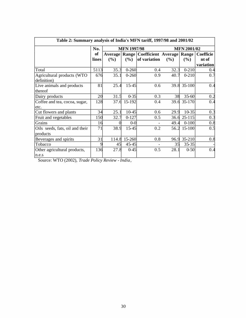
30

Table 2: Summary analysis of India's MFN tariff, 1997/98 and 2001/02

MFN 1997/98 MFN 2001/02 No. of

lines Average

(%) Range

(%) Coefficient of variation

Average (%)

Range (%)

Coefficient of

variation Total 5113 35.3 0-260 0.4 32.3 0-210 0.4Agricultural products (WTO definition)

676 35.1 0-260 0.9 40.7 0-210 0.7

Live animals and products thereof

81 25.4 15-45 0.6 39.8 35-100 0.4

Dairy products 20 31.5 0-35 0.3 38 35-60 0.2Coffee and tea, cocoa, sugar, etc.

128 37.6 15-192 0.4 39.6 35-170 0.4

Cut flowers and plants 34 25.1 10-45 0.6 29.9 10-35 0.3Fruit and vegetables 150 32.7 0-127 0.5 36.6 25-115 0.3Grains 16 0 0-0 - 49.4 0-100 0.8Oils seeds, fats, oil and their products

71 38.9 15-45 0.2 56.2 15-100 0.5

Beverages and spirits 31 114.8 15-260 0.8 96.9 35-210 0.8Tobacco 9 45 45-45 - 35 35-35 -Other agricultural products, n.e.s

136 27.8 0-45 0.5 28.1 0-50 0.4

Source: WTO (2002), Trade Policy Review - India ,

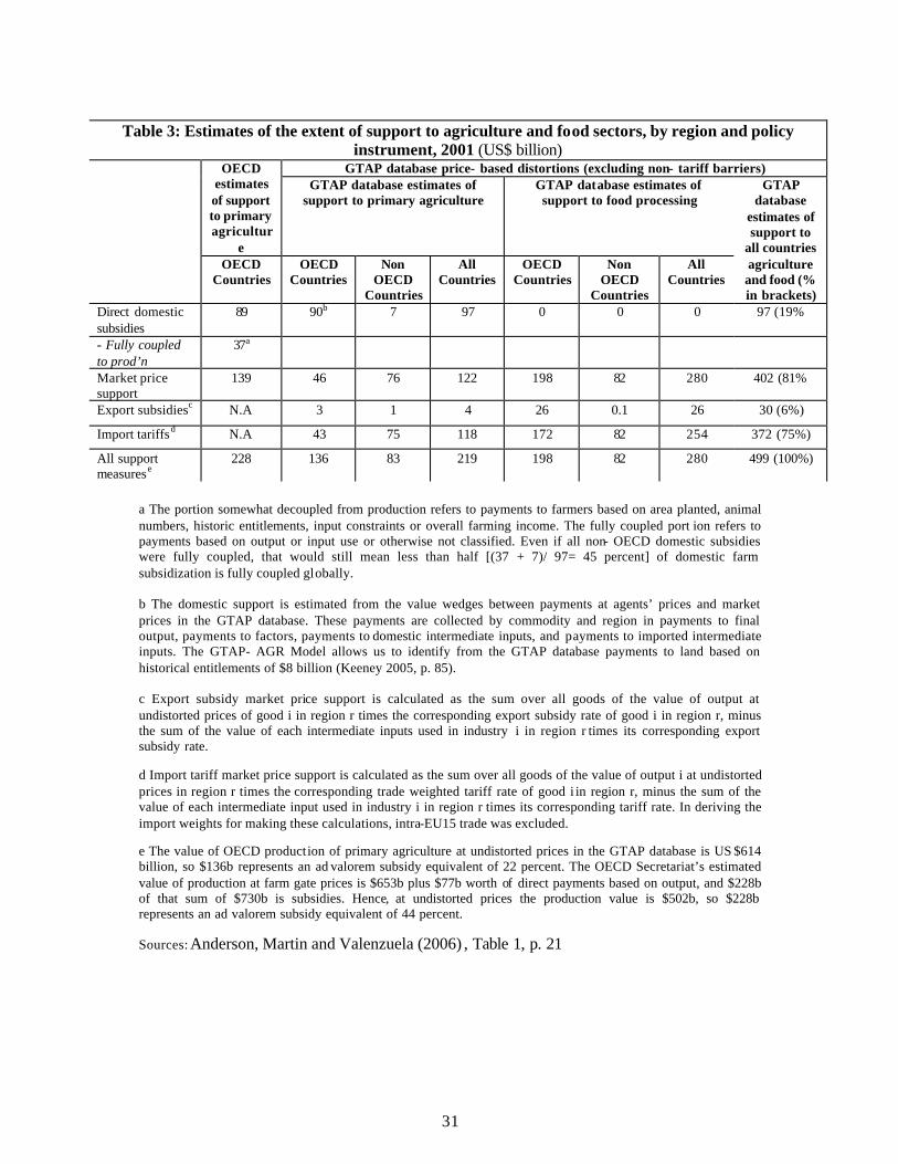
31

Table 3: Estimates of the extent of support to agriculture and food sectors, by region and policy

instrument, 2001 (US$ billion) GTAP database price- based distortions (excluding non- tariff barriers) OECD

estimates of support to primary agricultur

e

GTAP database estimates of support to primary agriculture

GTAP database estimates of support to food processing

OECD Countries

OECD Countries

Non OECD

Countries

All Countries

OECD Countries

Non OECD

Countries

All Countries

GTAP database

estimates of support to

all countries agriculture and food (% in brackets)

Direct domestic subsidies

89 90b 7 97 0 0 0 97 (19%

- Fully coupled to prod’n

37a

Market price support

139 46 76 122 198 82 280 402 (81%

Export subsidiesc N.A 3 1 4 26 0.1 26 30 (6%)

Import tariffsd N.A 43 75 118 172 82 254 372 (75%)

All support measurese

228 136 83 219 198 82 280 499 (100%)

a The portion somewhat decoupled from production refers to payments to farmers based on area planted, animal numbers, historic entitlements, input constraints or overall farming income. The fully coupled port ion refers to payments based on output or input use or otherwise not classified. Even if all non- OECD domestic subsidies were fully coupled, that would still mean less than half [(37 + 7)/ 97= 45 percent] of domestic farm subsidization is fully coupled globally. b The domestic support is estimated from the value wedges between payments at agents’ prices and market prices in the GTAP database. These payments are collected by commodity and region in payments to final output, payments to factors, payments to domestic intermediate inputs, and payments to imported intermediate inputs. The GTAP- AGR Model allows us to identify from the GTAP database payments to land based on historical entitlements of $8 billion (Keeney 2005, p. 85). c Export subsidy market price support is calculated as the sum over all goods of the value of output at undistorted prices of good i in region r times the corresponding export subsidy rate of good i in region r, minus the sum of the value of each intermediate inputs used in industry i in region r times its corresponding export subsidy rate.

d Import tariff market price support is calculated as the sum over all goods of the value of output i at undistorted prices in region r times the corresponding trade weighted tariff rate of good i in region r, minus the sum of the value of each intermediate input used in industry i in region r times its corresponding tariff rate. In deriving the import weights for making these calculations, intra-EU15 trade was excluded.

e The value of OECD production of primary agriculture at undistorted prices in the GTAP database is US $614 billion, so $136b represents an ad valorem subsidy equivalent of 22 percent. The OECD Secretariat’s estimated value of production at farm gate prices is $653b plus $77b worth of direct payments based on output, and $228b of that sum of $730b is subsidies. Hence, at undistorted prices the production value is $502b, so $228b represents an ad valorem subsidy equivalent of 44 percent.

Sources: Anderson, Martin and Valenzuela (2006) , Table 1, p. 21

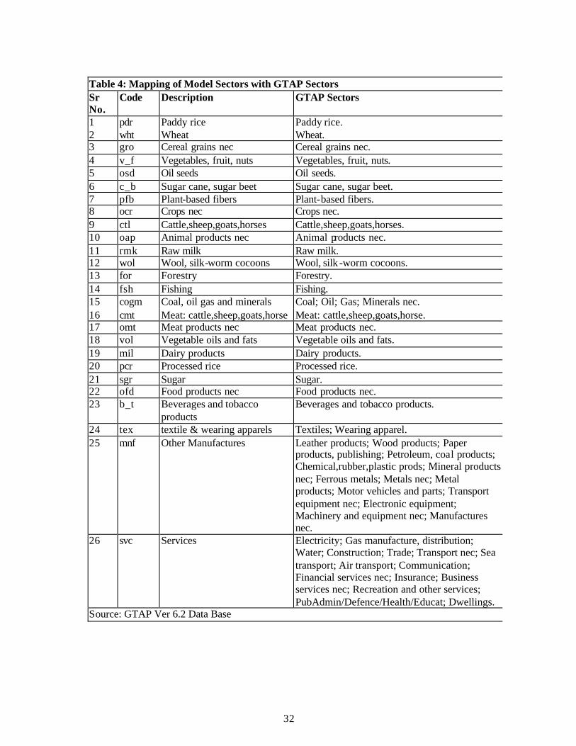
32

Table 4: Mapping of Model Sectors with GTAP Sectors Sr No.

Code Description GTAP Sectors

1 pdr Paddy rice Paddy rice. 2 wht Wheat Wheat. 3 gro Cereal grains nec Cereal grains nec. 4 v_f Vegetables, fruit, nuts Vegetables, fruit, nuts. 5 osd Oil seeds Oil seeds. 6 c_b Sugar cane, sugar beet Sugar cane, sugar beet. 7 pfb Plant-based fibers Plant-based fibers. 8 ocr Crops nec Crops nec. 9 ctl Cattle,sheep,goats,horses Cattle,sheep,goats,horses. 10 oap Animal products nec Animal products nec. 11 rmk Raw milk Raw milk. 12 wol Wool, silk-worm cocoons Wool, silk -worm cocoons. 13 for Forestry Forestry. 14 fsh Fishing Fishing. 15 cogm Coal, oil gas and minerals Coal; Oil; Gas; Minerals nec. 16 cmt Meat: cattle,sheep,goats,horse Meat: cattle,sheep,goats,horse. 17 omt Meat products nec Meat products nec. 18 vol Vegetable oils and fats Vegetable oils and fats. 19 mil Dairy products Dairy products. 20 pcr Processed rice Processed rice. 21 sgr Sugar Sugar. 22 ofd Food products nec Food products nec. 23 b_t Beverages and tobacco

products Beverages and tobacco products.

24 tex textile & wearing apparels Textiles; Wearing apparel. 25 mnf Other Manufactures Leather products; Wood products; Paper

products, publishing; Petroleum, coal products; Chemical,rubber,plastic prods; Mineral products nec; Ferrous metals; Metals nec; Metal products; Motor vehicles and parts; Transport equipment nec; Electronic equipment; Machinery and equipment nec; Manufactures nec.

26 svc Services Electricity; Gas manufacture, distribution; Water; Construction; Trade; Transport nec; Sea transport; Air transport; Communication; Financial services nec; Insurance; Business services nec; Recreation and other services; PubAdmin/Defence/Health/Educat; Dwellings.

Source: GTAP Ver 6.2 Data Base

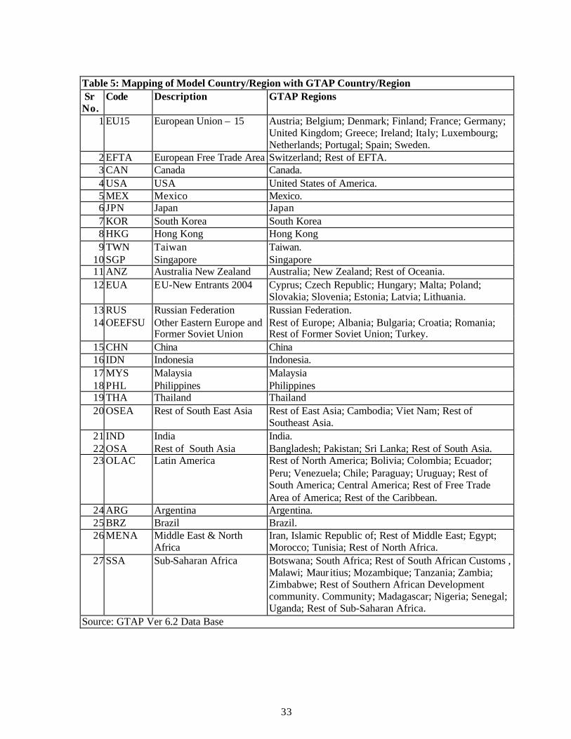
33

Table 5: Mapping of Model Country/Region with GTAP Country/Region Sr No.

Code Description GTAP Regions

1 EU15 European Union – 15 Austria; Belgium; Denmark; Finland; France; Germany; United Kingdom; Greece; Ireland; Italy; Luxembourg; Netherlands; Portugal; Spain; Sweden.

2 EFTA European Free Trade Area Switzerland; Rest of EFTA. 3 CAN Canada Canada. 4 USA USA United States of America. 5 MEX Mexico Mexico. 6 JPN Japan Japan 7 KOR South Korea South Korea 8 HKG Hong Kong Hong Kong 9 TWN Taiwan Taiwan.

10 SGP Singapore Singapore 11 ANZ Australia New Zealand Australia; New Zealand; Rest of Oceania. 12 EUA EU-New Entrants 2004 Cyprus; Czech Republic; Hungary; Malta; Poland;

Slovakia; Slovenia; Estonia; Latvia; Lithuania. 13 RUS Russian Federation Russian Federation. 14 OEEFSU Other Eastern Europe and

Former Soviet Union Rest of Europe; Albania; Bulgaria; Croatia; Romania; Rest of Former Soviet Union; Turkey.

15 CHN China China 16 IDN Indonesia Indonesia. 17 MYS Malaysia Malaysia 18 PHL Philippines Philippines 19 THA Thailand Thailand 20 OSEA Rest of South East Asia Rest of East Asia; Cambodia; Viet Nam; Rest of

Southeast Asia. 21 IND India India. 22 OSA Rest of South Asia Bangladesh; Pakistan; Sri Lanka; Rest of South Asia. 23 OLAC Latin America Rest of North America; Bolivia; Colombia; Ecuador;

Peru; Venezuela; Chile; Paraguay; Uruguay; Rest of South America; Central America; Rest of Free Trade Area of America; Rest of the Caribbean.

24 ARG Argentina Argentina. 25 BRZ Brazil Brazil. 26 MENA Middle East & North

Africa Iran, Islamic Republic of; Rest of Middle East; Egypt; Morocco; Tunisia; Rest of North Africa.

27 SSA Sub-Saharan Africa Botswana; South Africa; Rest of South African Customs , Malawi; Maur itius; Mozambique; Tanzania; Zambia; Zimbabwe; Rest of Southern African Development community. Community; Madagascar; Nigeria; Senegal; Uganda; Rest of Sub-Saharan Africa.

Source: GTAP Ver 6.2 Data Base

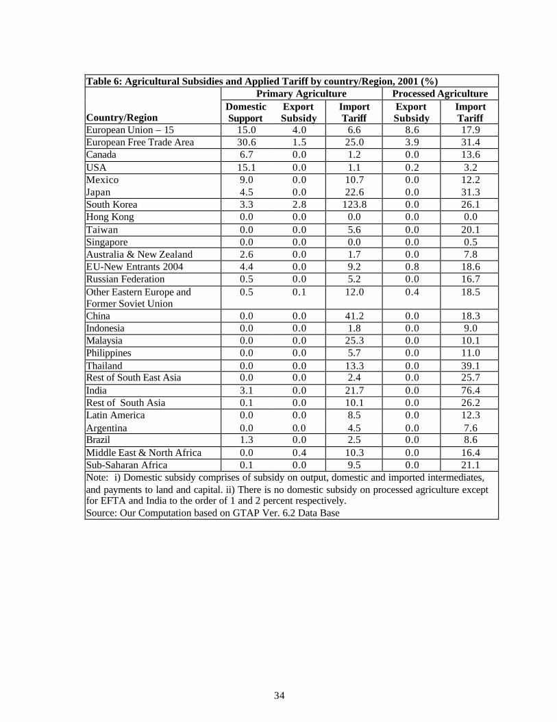
34

Table 6: Agricultural Subsidies and Applied Tariff by country/Region, 2001 (%)

Primary Agriculture Processed Agriculture

Country/Region Domestic Support

Export Subsidy

Import Tariff

Export Subsidy

Import Tariff

European Union – 15 15.0 4.0 6.6 8.6 17.9 European Free Trade Area 30.6 1.5 25.0 3.9 31.4 Canada 6.7 0.0 1.2 0.0 13.6 USA 15.1 0.0 1.1 0.2 3.2 Mexico 9.0 0.0 10.7 0.0 12.2 Japan 4.5 0.0 22.6 0.0 31.3 South Korea 3.3 2.8 123.8 0.0 26.1 Hong Kong 0.0 0.0 0.0 0.0 0.0 Taiwan 0.0 0.0 5.6 0.0 20.1 Singapore 0.0 0.0 0.0 0.0 0.5 Australia & New Zealand 2.6 0.0 1.7 0.0 7.8 EU-New Entrants 2004 4.4 0.0 9.2 0.8 18.6 Russian Federation 0.5 0.0 5.2 0.0 16.7 Other Eastern Europe and Former Soviet Union

0.5 0.1 12.0 0.4 18.5

China 0.0 0.0 41.2 0.0 18.3 Indonesia 0.0 0.0 1.8 0.0 9.0 Malaysia 0.0 0.0 25.3 0.0 10.1 Philippines 0.0 0.0 5.7 0.0 11.0 Thailand 0.0 0.0 13.3 0.0 39.1 Rest of South East Asia 0.0 0.0 2.4 0.0 25.7 India 3.1 0.0 21.7 0.0 76.4 Rest of South Asia 0.1 0.0 10.1 0.0 26.2 Latin America 0.0 0.0 8.5 0.0 12.3 Argentina 0.0 0.0 4.5 0.0 7.6 Brazil 1.3 0.0 2.5 0.0 8.6 Middle East & North Africa 0.0 0.4 10.3 0.0 16.4 Sub-Saharan Africa 0.1 0.0 9.5 0.0 21.1 Note: i) Domestic subsidy comprises of subsidy on output, domestic and imported intermediates, and payments to land and capital. ii) There is no domestic subsidy on processed agriculture except for EFTA and India to the order of 1 and 2 percent respectively. Source: Our Computation based on GTAP Ver. 6.2 Data Base

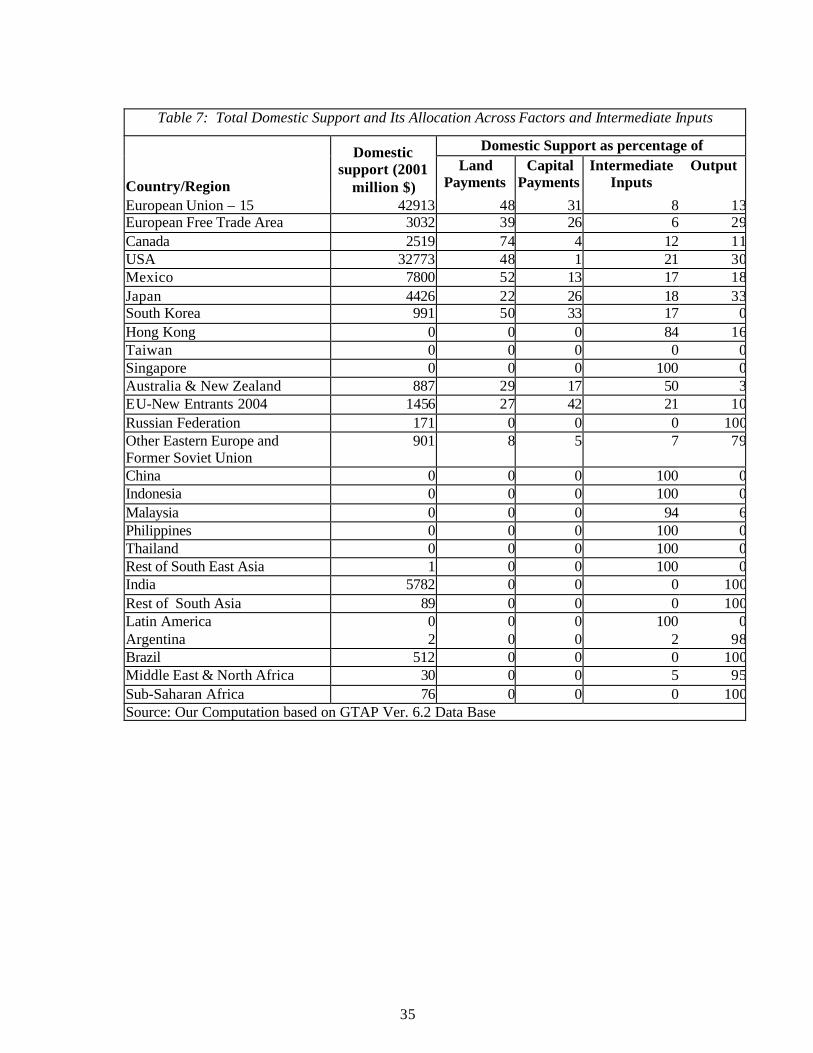
35

Table 7: Total Domestic Support and Its Allocation Across Factors and Intermediate Inputs

Domestic Support as percentage of

Country/Region

Domestic support (2001

million $) Land

Payments Capital

Payments Intermediate

Inputs Output

European Union – 15 42913 48 31 8 13European Free Trade Area 3032 39 26 6 29Canada 2519 74 4 12 11USA 32773 48 1 21 30Mexico 7800 52 13 17 18Japan 4426 22 26 18 33South Korea 991 50 33 17 0Hong Kong 0 0 0 84 16Taiwan 0 0 0 0 0Singapore 0 0 0 100 0Australia & New Zealand 887 29 17 50 3EU-New Entrants 2004 1456 27 42 21 10Russian Federation 171 0 0 0 100Other Eastern Europe and Former Soviet Union

901 8 5 7 79

China 0 0 0 100 0Indonesia 0 0 0 100 0Malaysia 0 0 0 94 6Philippines 0 0 0 100 0Thailand 0 0 0 100 0Rest of South East Asia 1 0 0 100 0India 5782 0 0 0 100Rest of South Asia 89 0 0 0 100Latin America 0 0 0 100 0Argentina 2 0 0 2 98Brazil 512 0 0 0 100Middle East & North Africa 30 0 0 5 95Sub-Saharan Africa 76 0 0 0 100Source: Our Computation based on GTAP Ver. 6.2 Data Base

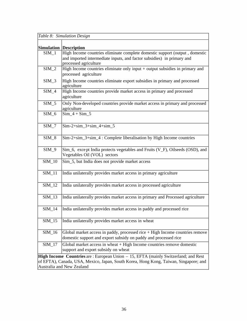
36

Table 8: Simulation Design Simulation Description

SIM_1 High Income countries eliminate complete domestic support (output , domestic and imported intermediate inputs, and factor subsidies) in primary and processed agriculture

SIM_2 High Income countries eliminate only input + output subsidies in primary and processed agriculture

SIM_3 High Income countries eliminate export subsidies in primary and processed agriculture

SIM_4 High Income countries provide market access in primary and processed agriculture

SIM_5 Only Non-developed countries provide market access in primary and processed agriculture

SIM_6 Sim_4 + Sim_5

SIM_7 Sim-2+sim_3+sim_4+sim_5

SIM_8 Sim-2+sim_3+sim_4 : Complete liberalisation by High Income countries

SIM_9 Sim_6, except India protects vegetables and Fruits (V_F), Oilseeds (OSD), and Vegetables Oil (VOL) sectors

SIM_10 Sim_5, but India does not provide market access

SIM_11 India unilaterally provides market access in primary agriculture

SIM_12 India unilaterally provides market access in processed agriculture

SIM_13 India unilaterally provides market access in primary and Processed agriculture

SIM_14 India unilaterally provides market access in paddy and processed rice

SIM_15 India unilaterally provides market access in wheat

SIM_16 Global market access in paddy, processed rice + High Income countries remove domestic support and export subsidy on paddy and processed rice

SIM_17 Global market access in wheat + High Income countries remove domestic support and export subsidy on wheat

High Income Countries are : European Union – 15, EFTA (mainly Switzerland; and Rest of EFTA), Canada, USA, Mexico, Japan, South Korea, Hong Kong, Taiwan, Singapore; and Australia and New Zealand

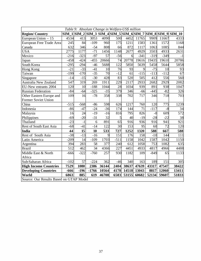
37

Table 9: Absolute Change in Welfare-US$ million

Region/ Country SIM_1 SIM_2 SIM_3 SIM_4 SIM_5 SIM_6 SIM_7 SIM_8 SIM_9 SIM_10 European Union – 15 4534 413 3053 4090 500 4452 11765 9909 11667 4333 European Free Trade Area 245 84 -109 960 175 1211 1583 1361 1572 1168 Canada 632 346 -54 808 66 872 1117 1063 1085 844 USA 2775 1177 -71 1456 1148 2677 4929 3503 4933 2631 Mexico -216 -323 -97 57 -56 6 -341 -319 -349 -1 Japan -458 -424 -455 20666 74 20778 19616 19435 19610 20786 South Korea -295 -294 -46 5688 122 5850 5639 5458 5644 5858 Hong Kong -21 -33 -41 10 76 93 9 -75 10 93 Taiwan -199 -170 -35 70 -12 61 -115 -113 -112 67 Singapore -14 -15 -30 428 83 520 505 412 556 560 Australia New Zealand 547 319 269 1911 229 2117 2933 2682 2929 2082 EU-New entrants 2004 120 10 -188 1044 28 1034 939 891 938 1047 Russian Federation -84 -64 -325 -35 379 346 -66 -445 -82 326 Other Eastern Europe and Former Soviet Union

109 16 -78 358 338 702 717 346 718 703

China -515 -568 -86 598 626 1217 760 120 775 1239 Indonesia -86 -47 -24 -36 174 144 71 -117 -8 34 Malaysia 16 24 -19 -16 816 795 826 -0 609 572 Philippines -69 -20 -31 32 5 40 -19 -28 -22 38 Thailand -23 -1 6 891 65 916 936 916 941 921 Rest of South East Asia -68 -41 -14 122 30 153 95 60 72 120 India 44 15 10 533 727 1252 1320 588 667 588 Rest of South Asia -38 -13 -16 9 151 176 158 -10 144 111 Latin America -209 14 -109 1703 -511 1158 1042 1587 1042 1150 Argentina 394 283 58 377 240 612 1058 753 1082 635 Brazil 512 462 34 4366 227 4451 4933 4817 4966 4488 Middle East & North Africa

-666 -322 -760 257 930 1182 109 -849 65 1133

Sub-Saharan Africa -102 57 -224 362 -46 340 163 189 151 305 High Income Countries 7529 1080 2386 36144 2404 38637 47639 43317 47547 38422 Developing Countries -666 -196 -1766 10564 4178 14518 13043 8817 12060 13411 World 6863 885 619 46708 6583 53155 60682 52134 59607 51833 Source: Our Results Based on GTAP Model

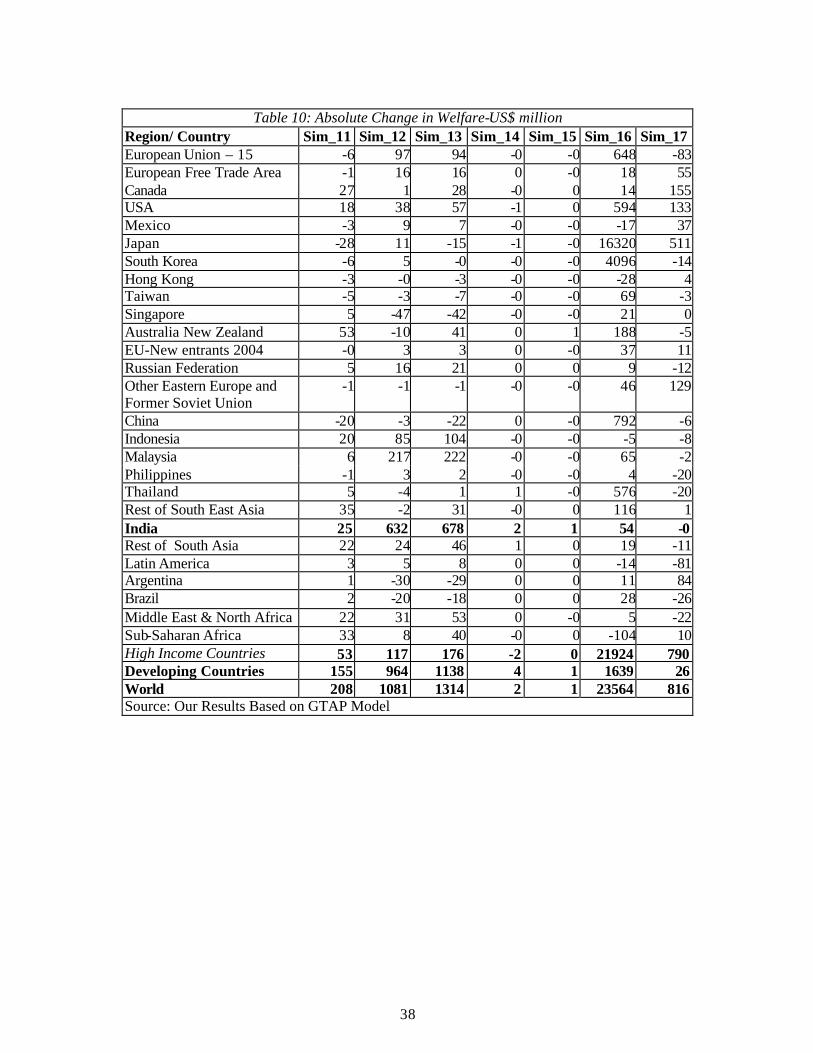
38

Table 10: Absolute Change in Welfare-US$ million

Region/ Country Sim_11 Sim_12 Sim_13 Sim_14 Sim_15 Sim_16 Sim_17 European Union – 15 -6 97 94 -0 -0 648 -83 European Free Trade Area -1 16 16 0 -0 18 55 Canada 27 1 28 -0 0 14 155 USA 18 38 57 -1 0 594 133 Mexico -3 9 7 -0 -0 -17 37 Japan -28 11 -15 -1 -0 16320 511 South Korea -6 5 -0 -0 -0 4096 -14 Hong Kong -3 -0 -3 -0 -0 -28 4 Taiwan -5 -3 -7 -0 -0 69 -3 Singapore 5 -47 -42 -0 -0 21 0 Australia New Zealand 53 -10 41 0 1 188 -5 EU-New entrants 2004 -0 3 3 0 -0 37 11 Russian Federation 5 16 21 0 0 9 -12 Other Eastern Europe and Former Soviet Union

-1 -1 -1 -0 -0 46 129

China -20 -3 -22 0 -0 792 -6 Indonesia 20 85 104 -0 -0 -5 -8 Malaysia 6 217 222 -0 -0 65 -2 Philippines -1 3 2 -0 -0 4 -20 Thailand 5 -4 1 1 -0 576 -20 Rest of South East Asia 35 -2 31 -0 0 116 1 India 25 632 678 2 1 54 -0 Rest of South Asia 22 24 46 1 0 19 -11 Latin America 3 5 8 0 0 -14 -81 Argentina 1 -30 -29 0 0 11 84 Brazil 2 -20 -18 0 0 28 -26 Middle East & North Africa 22 31 53 0 -0 5 -22 Sub-Saharan Africa 33 8 40 -0 0 -104 10 High Income Countries 53 117 176 -2 0 21924 790 Developing Countries 155 964 1138 4 1 1639 26 World 208 1081 1314 2 1 23564 816 Source: Our Results Based on GTAP Model

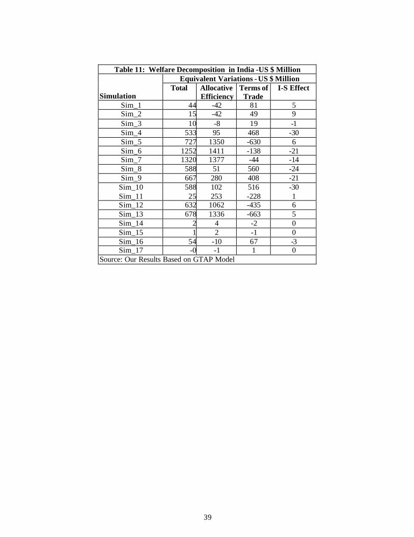
39

Table 11: Welfare Decomposition in India -US $ Million Equivalent Variations - US $ Million

Simulation Total

Allocative Efficiency

Terms of Trade

I-S Effect

Sim_1 44 -42 81 5 Sim_2 15 -42 49 9 Sim_3 10 -8 19 -1 Sim_4 533 95 468 -30 Sim_5 727 1350 -630 6 Sim_6 1252 1411 -138 -21 Sim_7 1320 1377 -44 -14 Sim_8 588 51 560 -24 Sim_9 667 280 408 -21

Sim_10 588 102 516 -30 Sim_11 25 253 -228 1 Sim_12 632 1062 -435 6 Sim_13 678 1336 -663 5 Sim_14 2 4 -2 0 Sim_15 1 2 -1 0 Sim_16 54 -10 67 -3 Sim_17 -0 -1 1 0

Source: Our Results Based on GTAP Model

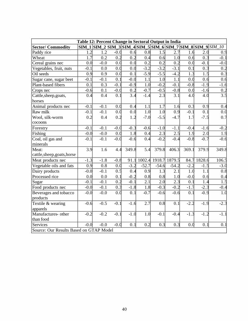
40

Table 12: Percent Change in Sectoral Output in India Sector/ Commodity SIM_1 SIM_2 SIM_3 SIM_4 SIM_5 SIM_6 SIM_7 SIM_8 SIM_9 SIM_10 Paddy rice 1.2 1.2 -0.0 0.6 0.8 1.5 2.7 1.6 2.0 0.9 Wheat 1.7 0.2 0.2 0.2 0.4 0.6 1.0 0.6 0.3 -0.1 Cereal grains nec 0.0 -0.0 0.0 0.0 0.2 0.2 0.2 0.0 -0.1 -0.0 Vegetables, fruit, nuts -0.1 0.0 0.0 0.0 -3.2 -3.2 -3.1 0.1 0.3 0.2 Oil seeds 0.9 0.9 0.0 0.1 -5.9 -5.5 -4.2 1.3 1.5 0.3 Sugar cane, sugar beet -0.1 -0.1 0.1 -0.0 1.1 1.0 1.1 0.0 0.6 0.6 Plant-based fibers 0.1 0.3 -0.1 -0.9 1.0 -0.2 -0.1 -0.8 -1.9 -1.6 Crops nec -0.6 0.1 -0.0 0.2 -0.7 -0.5 -0.8 0.0 -1.6 0.2 Cattle,sheep,goats, horses

0.4 0.4 0.1 3.4 -1.4 2.3 3.1 4.0 4.0 3.5

Animal products nec -0.1 -0.1 0.0 0.4 1.1 1.7 1.6 0.3 0.9 0.4 Raw milk -0.1 -0.1 0.0 0.0 1.0 1.0 0.9 -0.1 0.1 0.0 Wool, silk-worm cocoons

0.2 0.4 0.2 1.2 -7.0 -5.5 -4.7 1.7 -7.5 0.7

Forestry -0.1 -0.1 -0.0 -0.3 -0.6 -1.0 -1.1 -0.4 -1.6 -0.2 Fishing -0.0 -0.0 0.0 1.8 0.4 2.3 2.5 1.9 2.0 1.9 Coal, oil gas and minerals

-0.1 -0.1 -0.0 -0.6 0.4 -0.2 -0.4 -0.8 -0.7 -0.6

Meat: cattle,sheep,goats,horse

3.9 1.6 4.4 349.8 5.4 379.8 406.3 369.1 379.9 349.8

Meat products nec -1.3 -1.8 -0.8 91.1 1002.4 1918.7 1879.5 84.7 1828.6 106.5 Vegetable oils and fats 0.9 0.8 0.0 -3.2 -52.7 -54.6 -54.2 -2.2 -1.5 -3.0 Dairy products -0.0 -0.1 0.5 0.4 0.9 1.3 2.1 1.0 1.1 0.8 Processed rice 0.0 0.0 0.1 -0.2 0.8 0.8 1.0 -0.0 0.6 0.4 Sugar -0.1 -0.1 0.2 -0.1 2.1 2.0 2.3 0.1 1.4 1.5 Food products nec -0.0 -0.1 0.3 -1.8 1.8 -0.3 -0.2 -1.7 -2.3 -0.4 Beverages and tobacco products

-0.0 -0.0 0.0 0.1 -0.7 -0.6 -0.6 0.1 -0.9 1.0

Textile & wearing apparels

-0.6 -0.5 -0.1 -1.6 2.7 0.8 0.1 -2.2 -1.9 -2.3

Manufactures- other than food

-0.2 -0.2 -0.1 -1.0 1.0 -0.1 -0.4 -1.3 -1.2 -1.1

Services -0.0 -0.0 -0.0 0.1 0.2 0.3 0.3 0.0 0.1 0.1 Source: Our Results Based on GTAP Model

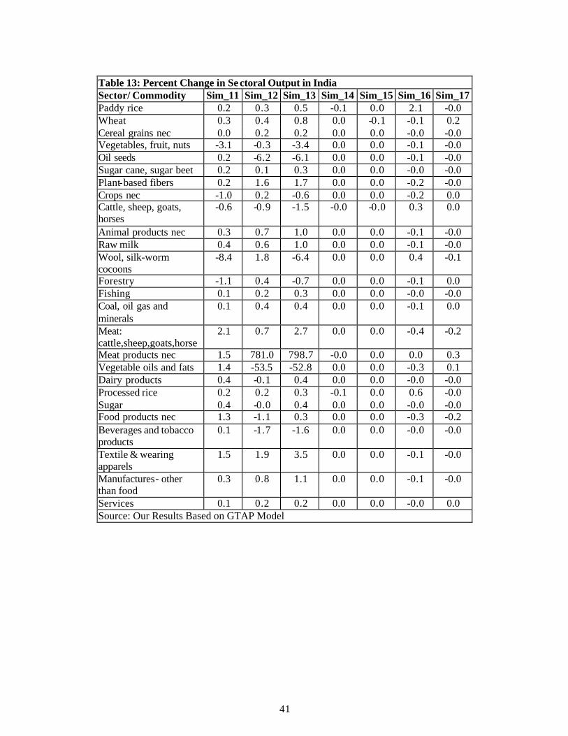
41

Table 13: Percent Change in Se ctoral Output in India Sector/ Commodity Sim_11 Sim_12 Sim_13 Sim_14 Sim_15 Sim_16 Sim_17 Paddy rice 0.2 0.3 0.5 -0.1 0.0 2.1 -0.0 Wheat 0.3 0.4 0.8 0.0 -0.1 -0.1 0.2 Cereal grains nec 0.0 0.2 0.2 0.0 0.0 -0.0 -0.0 Vegetables, fruit, nuts -3.1 -0.3 -3.4 0.0 0.0 -0.1 -0.0 Oil seeds 0.2 -6.2 -6.1 0.0 0.0 -0.1 -0.0 Sugar cane, sugar beet 0.2 0.1 0.3 0.0 0.0 -0.0 -0.0 Plant-based fibers 0.2 1.6 1.7 0.0 0.0 -0.2 -0.0 Crops nec -1.0 0.2 -0.6 0.0 0.0 -0.2 0.0 Cattle, sheep, goats, horses

-0.6 -0.9 -1.5 -0.0 -0.0 0.3 0.0

Animal products nec 0.3 0.7 1.0 0.0 0.0 -0.1 -0.0 Raw milk 0.4 0.6 1.0 0.0 0.0 -0.1 -0.0 Wool, silk-worm cocoons

-8.4 1.8 -6.4 0.0 0.0 0.4 -0.1

Forestry -1.1 0.4 -0.7 0.0 0.0 -0.1 0.0 Fishing 0.1 0.2 0.3 0.0 0.0 -0.0 -0.0 Coal, oil gas and minerals

0.1 0.4 0.4 0.0 0.0 -0.1 0.0

Meat: cattle,sheep,goats,horse

2.1 0.7 2.7 0.0 0.0 -0.4 -0.2

Meat products nec 1.5 781.0 798.7 -0.0 0.0 0.0 0.3 Vegetable oils and fats 1.4 -53.5 -52.8 0.0 0.0 -0.3 0.1 Dairy products 0.4 -0.1 0.4 0.0 0.0 -0.0 -0.0 Processed rice 0.2 0.2 0.3 -0.1 0.0 0.6 -0.0 Sugar 0.4 -0.0 0.4 0.0 0.0 -0.0 -0.0 Food products nec 1.3 -1.1 0.3 0.0 0.0 -0.3 -0.2 Beverages and tobacco products

0.1 -1.7 -1.6 0.0 0.0 -0.0 -0.0

Textile & wearing apparels

1.5 1.9 3.5 0.0 0.0 -0.1 -0.0

Manufactures- other than food

0.3 0.8 1.1 0.0 0.0 -0.1 -0.0

Services 0.1 0.2 0.2 0.0 0.0 -0.0 0.0 Source: Our Results Based on GTAP Model

42

References

Acharya, S.S. (2004), “Agricultural Marketing”, Volume 17 of the State of the Indian Farmer, Ministry of Agriculture and Academic Publishers, New Delhi.

Ackerman, Frank (2005), “The Shrinking Gains from Trade: A Critical Assessment of Doha Round Projections”, Working Paper No. 05-01, Global Development and Environment Institute, Tufts University, Medford.

Anderson, Kym and Will Martin (2006), “Scenarios for Global Trade Reform”, in Thomas Hertel and Will Martin (eds.), Poverty and the WTO, Chapter 2, New York: Palgrave Macmillan; Washington D.C: the World Bank.

Anderson, Kym, Will Martin and Ernesto Valenzuela (2006), “The Relative Importance of Global Agricultural Subsidies and Market Access”, World Bank. Forthcoming in World Trade Review 5(3), November 2006.

Ash, Ken (2006), “Agricultural Policies in Selected OECD Countries: Prospects for Reform”, Paris, Australian Commodities, Vol. 13, No. 1, Australia.

Bouet, Antoine, et al. (2005), “A Consistent ad-valorem measure of applied protection across the World: The MAcMAP HS-6 Database”, CEPII, Paris.

Brown, D.K., A.V. Deardorff and R.M. Sterns (2002), “Computational Analysis of Multilateral Trade Liberalization in the Uruguay Round and Doha Development Round”, RSIE Discussion paper No. 489 , School of Public Policy, University of Michigan, Ann Arbor.

Burfisher, Mary, E. (2003), “Options for Agricultural Policy Reform in the World Trade Organisation Negotiations”, in Merlinda D. Ingco (ed.), Agriculture, Trade and the WTO, Washington D.C.: The World Bank.

Chadha, Rajesh, Drusilla K. Brown, Alan V.Deardorff, and Robert M. Stern (2003). "Computational Analysis of the Impact on India of the Uruguay Round and the Doha Development Agenda Negotiations", in Aaditya Mattoo and Robert M. Stern (eds.), India and the WTO, Washington D.C.: Oxford University Press in collaboration with the World Bank.

Chadha, Rajesh, Pooja Sharma and Anjali Tandon (2005), “Liberalising Indian Agriculture”, Margin , 37(3), April-June.

Chand, Ramesh (1999), “Trade Liberalisation and Net Social Welfare: A Study of Selected Crops, Economic and Political Weekly , 1999, 52(34).

Chand, Ramesh (2003), “Agricultural Marketing and Trade in India: An Institutional Perspective”, in Suresh Pal, Mruthyunjaya, P.K. Joshi and Raka Saxena (eds.), Institutional Changes in Indian Agriculture, NCAP, New Delhi, pp. 345-368.

Chand, Ramesh (2005a), “Agricultural Markets in India: Implications for competition”, in Pradeep S. Mehta (ed.), Towards A Functional competition Policy for India , Chapter 11, New Delhi: Academic Foundation and Consumer unity Trust Society (CUTS), Jaipur

43

Chand, Ramesh (2005b), “India’s Agricultural Challenge and their Implications for Growth of its Economy”, Paper submitted for international symposium on Regional Integration in Asia and India”, IDE-JETRO, Tokyo Japan, 8 December 2005.

Chand, Ramesh and Mruthyunjaya (2006), Wto and Indian Agriculture: Implications for Policy and R &D”, Policy paper 38, National Academy of Agricultural Sciences (NAAS), New Delhi.

Charlton, Andre H. and Joseph E. Stiglitz (2005), “A Development -friendly Prioritisation of Doha Round Proposals”, The World Economy, Blackwell Publishing limited.

Diakosavva, D. (2003) “The Uruguay Round Agreement on Agriculture in Practice: How Open are OECD Markets?”, in Merlinda D. Ingco (ed.), Agriculture, Trade and the WTO. Washington D.C.: The World Bank.

Dimaranan, Betina, Thomas Hertel and Roman Keeney (2004), “OECD Domestic Support and Developing Countries”, in Basudev Guha-Khasnobis (ed.), The WTO, Developing Countries and the Doha Development Agenda: Prospects and Challenges for Trade-Led Growth, London: Palgrave -Macmillan.

Francois, J., H. van Meijl and F. van Tongeren (2005), “Trade Liberalisation in the Doha Development Round”, Economic Policy, 20(42): pp 340-391.

Government of India (1998-2000), “Bulletin on Food Statistics”, Department of Agriculture & Co-operation, Ministry of Agriculture.

Government of India (2000), “Important Markets of Major Agricultural Commodities in India”, Department of Agriculture & Co-operation, Directorate of Marketing & Inspection, Ministry of Agriculture, Branch Head Office, Nagpur.

Government of India (2001), “Expert Committee Report on Agricultural marketing”, Ministry of Agriculture.

Government of India (2002), “Report of The Inter-Ministerial Task Force on Agricultural Marketing Reforms”, Ministry of Agriculture.

Government of India (2003), “The Model Act: The State Agricultural Produce Marketing, Development & Regulation Act, 2003”, Ministry of Agriculture.

Government of India (2004), “Agricultural Statistics at a Glance, Agricultural Statistics Division, Department of Agriculture & Cooperation, Ministry of Agriculture, New Delhi.

Government of India (2004), “Economic Survey - 2003-04”, Ministry of Finance, Economic Division, New Delhi.

Government of India (2004), “Post Harvest Profile of Paddy/Rice”, Directorate of Marketing and Inspection, Branch Head Office, Department of Agriculture and Co-operation, Ministry of Agriculture, Nagpur.

Government of India (2004), “Reports of the Commission for Agricultural Costs and Prices - For the Crops Sown During 2003-04 Season”, Department of Agriculture and Co-operation, Ministry of Agriculture, New Delhi.

Government of India (2006), “Towards Faster and More Inclusive Growth: An Approach to the 11th Five Year Plan”, 14th June, Planning Commission, Ministry of Planning and Programme Implmentation, New Delhi.

44

Government of India, Ministry of Agriculture, Department of Agriculture & Co-operation, Directorate of Marketing and Inspection, Official website of AGMARKNET

Government of India, Ministry of Consumer Affairs, Food and Public Distribution

Harrison, W. J and Pearson, Ken (2005), GEMPACK User Documentation, Various Issue, Release 9.0, Centre of Policy Studies and Impact Project, Monash University, Clayton, Australia, October, 2002.

Hertel, Thomas (ed.) (1997), “Global Trade Analysis: Modelling and Applications”, cambridge university Press.

Hertel, Thomas and Roman Keeney (2006), “What is as Stake: The Relative Importance of Import Barriers, Export Subsidies and Domestic Support”, in Kym Anderson and Will Martin (eds.) Agricultural Trade Reform and the Doha Development Agenda, Chapter 2, New York: Palgrave Macmillan; Washington D C: the World Bank.

Huff, Karen and Thomas W. Hertel (1996), “Decomposing the Welfare Changes in the GTAP Model”, GTAP Technical Paper No. 15. Purdue University, West Lafayette, IN

Jensen, Hans G. (2005), “Domestic Support: The European Union” in Dimaranan, Betina V. and McDougall, Robert A. (eds), Global Trade, Assistance, and Production: The GTAP 6 Data Base Documentation, Center for Global Trade Analysis, Purdue University, West Lafayette, Indiana, USA, July 2005.

Jha, Veena, Kailas Karthikeyan and Abhijit Das (2006), Impact of Trade Liberalisation on Indian Agriculture”, in Veena Jha (ed) India and the Doha Work Programme: Opportunities and Challenges, Chapter 2, New Delhi: UNCTAD and Macmillan India.

Keeney, Roman and Thomas Hertel (2005), “GTAP-AGR: A Framework for Assessing the Implications of Multilateral Changes in Agricultural Policies”, GTAP Technical Paper No. 24. Purdue University, West Lafayette, IN.

Landes, Rip and Ashok Gulati (2004), “Farm Sector Performance and Reform Agenda”, Economic and Political Weekly , 39(32), Special Article, August 7, pp. 3611-19.

Lavoie, N. (2003), ‘The Impact of Reforming Wheat Importing State -Trading Enterprises on the Quality of Wheat Imported”, University of Massachusetts, Amherst Working Paper No. 2003-12.

McCorriston, S. and D. MacLaren (2005a), “The trade distorting effect of state trading enterprises in importing countries”, European Economic Review , 49 (7): pp. 1693-1715.

McCorriston, S. and D. MacLaren (2005b), “Single-desk state trading exporters”, European Journal of Political Economy, 21(2): pp. 503-524.

Messerlin, Patrick A. (2005), “Agriculture”, Paper presented at “Perspectives on the WTO Doha Development Agenda Multilateral Trade Negotiations”, Ann Arbor, Michigan Global Economy Journal, 5(4), Berkeley Electronic Press: http://www.bepress.com/gej

OECD (2004), “Agricultural Support: How is it Measured and What does it Mean?” OECD Observer, Paris.

45

OECD (2005), “Agricultural Policies in OECD Countries: Monitoring and Evaluation”, OECD, Paris.

Panagariya, Arvind (2005), “Liberalizing Agriculture”, Foreign Affairs, WTO Special Issue, December 2005.

Pant, Hom, Stephen Brown, Benjamin Buetre and Vivek Tulpule (2000), “Measurement and Decomposition of Welfare Changes in GTEM”, Third Annual Conference on Global Economic Analysis, Melbourne, June 2000.

Piermartini, Roberta and Robert The (2005), “ Demystyfying Modelling Methods for Trade Policy “, Discussion Paper No. 10, Geneva, Switzerland, WTO

Rae, A. and A. Strutt (2003), “Doha Proposals for Domestic Support: Assessing the Priorities”, paper presented at the Annual meeting of the International Trade Research Consortium.

Razzaque, Mohammad A., Selim Rehan and Nazneen Ahmed (2006), “Global Rice Trade Liberalisation: Implications for Some Alternative Scenarios”, 9th Annual Conference on Global Economic Analysis, Addis Ababa, Ethiopia.

Tangermann, Stefan (2005), “Is the Concept of the Producer Support Estimate in Need of Revision?”, OECD Food, Agriculture and Fisheries Working paper No. 1 , OECD, Paris.

Taylor, Lance and Rudiger von Arnim (2006), Modelling the Impact of Trade Liberalisation: A Critique of CGE Models”, Report Prepared fo r OXFAM International, New School for Social Research, New York.

Valenzuela, Ernesto, Kym Anderson and Thomas Hertel (2006), “Impacts of Trade Reform: Sensitivity of GTAP Results to Modelling Assumptions”, 9th Annual Conference on Global Economic Analysis, Addis Ababa, Ethiopia.

Veeman, M., Fulton, M., & B. Larue (1999), “International Trade in Agricultural and Food Products: The Role of State Trading Enterprises”, Economic and Policy Analysis Directorate. Agriculture and Agri-Food Canada.

Walsh, Keith, Martina Brockmeier and Alan Mathews (2005), “Implications of Domestic Support for Further Agricultural Trade Liberalisation”, 8th Annual Conference on Global Economic Analysis, Lubeck, Germany.

WTO (1995), The Results of the Uruguay Round of Multilateral Trade Negotiations: The Legal Texts, Geneva.

WTO (2002), Trade Policy Review: India.