Embed Size (px)
Citation preview
Introduction and stylized facts Derivation of new market formulas Extending the lognormal LIBOR Market Model
LIBOR Market Models with Stochastic Basis
Fabio Mercurio
Bloomberg, New York
Swissquote Conference on Interest Rate and Credit RiskLausanne, 28 October 2010

Introduction and stylized facts Derivation of new market formulas Extending the lognormal LIBOR Market Model
Stylized facts
• Before the credit crunch of 2007, interest rates in themarket showed typical textbook behavior. For instance:
• A (canonical) floating rate bond is worth par at inception.• The forward rate implied by two deposits coincides with the
corresponding FRA rate.• Compounding two consecutive 3m forward LIBOR rates
yields the corresponding 6m forward LIBOR rate.
• These properties allowed one to construct a well-definedzero-coupon curve.
• Then August 2007 arrived, and our convictions began towaver: The liquidity crisis widened the basis betweenpreviously-near rates.
• Consider the following graphs ...

Introduction and stylized facts Derivation of new market formulas Extending the lognormal LIBOR Market Model
USD Market quotesOvernight-indexed-swap rates and LIBORs
USD 3m OIS rates vs 3m Depo rates

Introduction and stylized facts Derivation of new market formulas Extending the lognormal LIBOR Market Model
USD Market quotesOvernight-indexed-swap rates and LIBORs
USD 6m OIS rates vs 6m Depo rates

Introduction and stylized facts Derivation of new market formulas Extending the lognormal LIBOR Market Model
USD Market quotesFRA rates and OIS forward rates
USD 3x6 FRA vs 3x6 fwd OIS

Introduction and stylized facts Derivation of new market formulas Extending the lognormal LIBOR Market Model
USD Market quotesInterest rate swaps with different frequencies
USD 5y swaps: 1m vs 3m

Introduction and stylized facts Derivation of new market formulas Extending the lognormal LIBOR Market Model
EUR Market quotesOvernight-indexed-swap rates and LIBORs
EUR 3m OIS rates vs 3m Depo rates

Introduction and stylized facts Derivation of new market formulas Extending the lognormal LIBOR Market Model
EUR Market quotesOvernight-indexed-swap rates and LIBORs
EUR 6m OIS rates vs 6m Depo rates
Introduction and stylized facts Derivation of new market formulas Extending the lognormal LIBOR Market Model
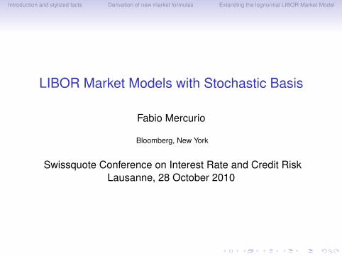
EUR Market quotesFRA rates and OIS forward rates
EUR 3x6 FRA vs 3x6 fwd OIS
Introduction and stylized facts Derivation of new market formulas Extending the lognormal LIBOR Market Model
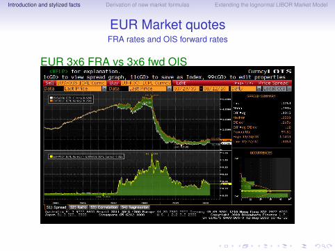
EUR Market quotesFRA rates and OIS forward rates
EUR 6x12 FRA vs 6x12 fwd OIS
Introduction and stylized facts Derivation of new market formulas Extending the lognormal LIBOR Market Model
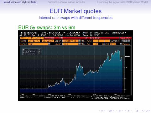
EUR Market quotesInterest rate swaps with different frequencies
EUR 5y swaps: 3m vs 6m
Introduction and stylized facts Derivation of new market formulas Extending the lognormal LIBOR Market Model
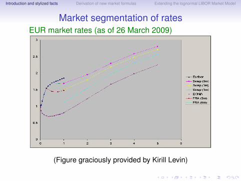
Market segmentation of ratesEUR market rates (as of 26 March 2009)
(Figure graciously provided by Kirill Levin)
Introduction and stylized facts Derivation of new market formulas Extending the lognormal LIBOR Market Model
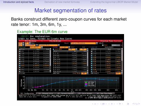
Market segmentation of ratesBanks construct different zero-coupon curves for each marketrate tenor: 1m, 3m, 6m, 1y, ...
Example: The EUR 6m curve

Introduction and stylized facts Derivation of new market formulas Extending the lognormal LIBOR Market Model
The discount curve
• We take the OIS zero-coupon curve, stripped from marketOIS swap rates, as the discount curve:
T 7→ PD(0,T ) = POIS(0,T )
• The rationale behind this is that in the interbank derivativesmarket, a collateral agreement (CSA) is often negotiatedbetween the two counterparties.
• We assume here that the collateral is revalued daily at arate equal to the overnight rate.
• If the CSA reduces the counterparty risk to zero, it makessense to discount with OIS rates since they can beregarded as risk-free.
• The OIS curve can be stripped from OIS swap rates usingstandard (single-curve) bootstrapping methods.
Introduction and stylized facts Derivation of new market formulas Extending the lognormal LIBOR Market Model
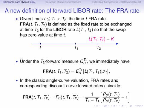
A new definition of forward LIBOR rate: The FRA rate• Given times t ≤ T1 < T2, the time-t FRA rate
FRA(t ; T1,T2) is defined as the fixed rate to be exchangedat time T2 for the LIBOR rate L(T1,T2) so that the swaphas zero value at time t .
-
t T1 T2
L(T1,T2)− K
• Under the T2-forward measure QT2D , we immediately have
FRA(t ; T1,T2) = ET2D
[L(T1,T2)|Ft
],
• In the classic single-curve valuation, FRA rates andcorresponding discount-curve forward rates coincide:
FRA(t ; T1,T2) = FD(t ; T1,T2) =1
T2 − T1
[PD(t ,T1)
PD(t ,T2)− 1
]

Introduction and stylized facts Derivation of new market formulas Extending the lognormal LIBOR Market Model
A new definition of forward LIBOR rate: The FRA rate• In fact, in the single-curve case L(T1,T2) is defined by the
classic relation
L(T1,T2) =1
T2 − T1
[1
PD(T1,T2)− 1
]= FD(T1; T1,T2),
so that
ET2D
[L(T1,T2)|Ft
]= FRA(t ; T1,T2)
= ET2D
[FD(T1; T1,T2)|Ft
]= FD(t ; T1,T2)
• In our dual-curve setting, however,
L(T1,T2) 6= FD(T1; T1,T2) = LOIS(T1,T2)
implying that
FRA(t ; T1,T2) 6= FD(t ; T1,T2)

Introduction and stylized facts Derivation of new market formulas Extending the lognormal LIBOR Market Model
A new definition of forward LIBOR rate: The FRA rate
The FRA rate above is the natural generalization of a forwardrate to the dual-curve case.In fact:
1. The FRA rate coincides with the classically-defined forwardrate.
2. At its reset time T1, the FRA rate FRA(T1; T1,T2) coincideswith the LIBOR rate L(T1,T2).
3. The FRA rate is a martingale under the correspondingforward measure.
4. Its time-0 value FRA(0; T1,T2) can be stripped frommarket data.
• These properties will prove to be very convenient whenpricing swaps and options on LIBOR/swap rates.

Introduction and stylized facts Derivation of new market formulas Extending the lognormal LIBOR Market Model
The valuation of interest rate swaps (IRSs)(under the assumption of distinct forward and discount curves)
• Given times Ta, . . . ,Tb, consider an IRS whose floating legpays at each Tk the LIBOR rate with tenor Tk − Tk−1,which is set (in advance) at Tk−1, i.e.
τkL(Tk−1,Tk )
where τk denotes the year fraction.• The time-t value of this payoff is:
FL(t ; Tk−1,Tk ) = τkPD(t ,Tk )ETkD
[L(Tk−1,Tk )|Ft
]=: τkPD(t ,Tk )Lk (t)
where Lk (t) := FRA(t ; Tk−1,Tk ).• The swap’s fixed leg is assumed to pay the fixed rate K on
dates T Sc , . . . ,T S
d , with year fractions τSj .

Introduction and stylized facts Derivation of new market formulas Extending the lognormal LIBOR Market Model
The valuation of interest rate swaps (cont’d)
• The IRS value to the fixed-rate payer is given by
IRS(t ,K ) =b∑
k=a+1
τkPD(t ,Tk )Lk (t)− Kd∑
j=c+1
τSj PD(t ,T S
j )
• We can then calculate the corresponding forward swaprate as the fixed rate K that makes the IRS value equal tozero at time t . At t = 0, we get:
S0,b,0,d(0) =
∑bk=1 τkPD(0,Tk )Lk (0)∑d
j=1 τSj PD(0,T S
j )
where L1(0) is the first floating payment (known at time 0).

Introduction and stylized facts Derivation of new market formulas Extending the lognormal LIBOR Market Model
The valuation of interest rate swaps (cont’d)
• In practice, this swap rate formula can be used to bootstrapthe rates Lk (0).
• The bootstrapped Lk (0) can then be used to price otherswaps based on the given tenor.
Swap rate Formulas
OLD∑b
k=1 τk P(0,Tk )Fk (0)∑dj=1 τS
j P(0,T Sj )
=1−P(0,T S
d )∑dj=1 τS
j P(0,T Sj )
NEW∑b
k=1 τk PD(0,Tk )Lk (0)∑dj=1 τS
j PD(0,T Sj )

Introduction and stylized facts Derivation of new market formulas Extending the lognormal LIBOR Market Model
The valuation of caplets
• Let us consider a caplet paying out at time Tk
τk [L(Tk−1,Tk )− K ]+.
• The caplet price at time t is given by:
Cplt(t ,K ; Tk−1,Tk ) = τkPD(t ,Tk )ETkD
{[L(Tk−1,Tk )− K ]+|Ft
}= τkPD(t ,Tk )ETk
D
{[Lk (Tk−1)− K ]+|Ft
}• The FRA rate Lk (t) = ETk
D [L(Tk−1,Tk )|Ft ] is, by definition,a martingale under QTk
D .• Assume that Lk follows a (driftless) geometric Brownian
motion under QTkD .
• Straightforward calculations lead to a (modified) Blackformula for caplets.

Introduction and stylized facts Derivation of new market formulas Extending the lognormal LIBOR Market Model
The valuation of swaptions• A payer swaption gives the right to enter at time Ta = T S
can IRS with payment times for the floating and fixed legsgiven by Ta+1, . . . ,Tb and T S
c+1, . . . ,TSd , respectively.
• Therefore, the swaption payoff at time Ta = T Sc is
[Sa,b,c,d(Ta)− K
]+d∑
j=c+1
τSj PD(T S
c ,TSj ),
where K is the fixed rate and
Sa,b,c,d(t) =
∑bk=a+1 τkPD(t ,Tk )Lk (t)∑d
j=c+1 τSj PD(t ,T S
j )
• Assume that Sa,b,c,d is a (lognormal) martingale under theassociated swap measure.
• We thus obtain a (modified) Black formula for swaptions.

Introduction and stylized facts Derivation of new market formulas Extending the lognormal LIBOR Market Model
The new market formulas for caps and swaptions
Type Formulas
OLD Cplt τkP(t ,Tk ) Bl(K ,Fk (t), vk
√Tk−1 − t
)NEW Cplt τkPD(t ,Tk ) Bl
(K ,Lk (t), v̄k
√Tk−1 − t
)
OLD PS∑d
j=c+1 τSj P(t ,T S
j ) Bl(K ,SOLD(t), ν
√Ta − t
)
NEW PS∑d
j=c+1 τSj PD(t ,T S
j ) Bl(K ,Sa,b,c,d(t), ν̄
√Ta − t
)
Introduction and stylized facts Derivation of new market formulas Extending the lognormal LIBOR Market Model
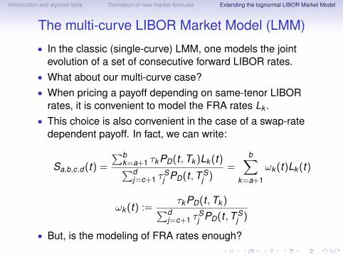
The multi-curve LIBOR Market Model (LMM)
• In the classic (single-curve) LMM, one models the jointevolution of a set of consecutive forward LIBOR rates.
• What about our multi-curve case?• When pricing a payoff depending on same-tenor LIBOR
rates, it is convenient to model the FRA rates Lk .• This choice is also convenient in the case of a swap-rate
dependent payoff. In fact, we can write:
Sa,b,c,d(t) =
∑bk=a+1 τkPD(t ,Tk )Lk (t)∑d
j=c+1 τSj PD(t ,T S
j )=
b∑k=a+1
ωk (t)Lk (t)
ωk (t) :=τkPD(t ,Tk )∑d
j=c+1 τSj PD(t ,T S
j )
• But, is the modeling of FRA rates enough?

Introduction and stylized facts Derivation of new market formulas Extending the lognormal LIBOR Market Model
The multi-curve LIBOR Market Model (LMM)Alternative formulations
• In fact, we also need to model the OIS forward rates,k = 1, . . . ,M:
Fk (t) := FD(t ; Tk−1,Tk ) =1τk
[PD(t ,Tk−1)
PD(t ,Tk )− 1
]• Denote by Sk (t) the spread
Sk (t) := Lk (t)− Fk (t)
• By definition, both Lk and Fk are martingales under theforward measure QTk
D , and thus their difference Sk is aswell.
• The LMM can be extended to the multi-curve case in threedifferent ways by:
1. Modeling the joint evolution of rates Lk and Fk .2. Modeling the joint evolution of rates Lk and spreads Sk .3. Modeling the joint evolution of rates Fk and spreads Sk .
Introduction and stylized facts Derivation of new market formulas Extending the lognormal LIBOR Market Model
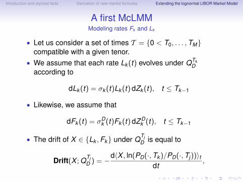
A first McLMMModeling rates Fk and Lk
• Let us consider a set of times T = {0 < T0, . . . ,TM}compatible with a given tenor.
• We assume that each rate Lk (t) evolves under QTkD
according to
dLk (t) = σk (t)Lk (t) dZk (t), t ≤ Tk−1
• Likewise, we assume that
dFk (t) = σDk (t)Fk (t) dZ D
k (t), t ≤ Tk−1
• The drift of X ∈ {Lk ,Fk} under QTjD is equal to
Drift(X ; QTjD ) = −
d〈X , ln(PD(·,Tk )/PD(·,Tj))〉tdt
,

Introduction and stylized facts Derivation of new market formulas Extending the lognormal LIBOR Market Model
A first McLMMDynamics under a general forward measure
Proposition. The dynamics of Lk and Fk under QTjD are:
j < k :
dLk (t) = σk (t)Lk (t)
[k∑
h=j+1
ρL,Fk,h τ
Dh σ
Dh (t)Fh(t)
1 + τDh Fh(t)
dt + dZ jk (t)
]
dFk (t) = σDk (t)Fk (t)
[k∑
h=j+1
ρD,Dk,h τ
Dh σ
Dh (t)Fh(t)
1 + τDh Fh(t)
dt + dZ j,Dk (t)
]
j = k :
{dLk (t) = σk (t)Lk (t) dZ j
k (t)dFk (t) = σD
k (t)Fk (t) dZ j,Dk (t)
j > k :
dLk (t) = σk (t)Lk (t)
[−
j∑h=k+1
ρL,Fk,h τ
Dh σ
Dh (t)Fh(t)
1 + τDh Fh(t)
dt + dZ jk (t)
]
dFk (t) = σDk (t)Fk (t)
[−
j∑h=k+1
ρD,Dk,h τ
Dh σ
Dh (t)Fh(t)
1 + τDh Fh(t)
dt + dZ j,Dk (t)
]
Introduction and stylized facts Derivation of new market formulas Extending the lognormal LIBOR Market Model
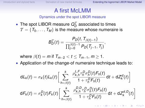
A first McLMMDynamics under the spot LIBOR measure
• The spot LIBOR measure QTD associated to times
T = {T0, . . . ,TM} is the measure whose numeraire is
BTD (t) =PD(t ,Tβ(t)−1)∏β(t)−1
j=0 PD(Tj−1,Tj),
where β(t) = m if Tm−2 < t ≤ Tm−1, m ≥ 1.• Application of the change-of numeraire technique leads to:
dLk (t) = σk (t)Lk (t)[ k∑
h=β(t)
ρL,Fk ,h τ
Dh σ
Dh (t)Fh(t)
1 + τDh Fh(t)
dt + dZ dk (t)
]
dFk (t) = σDk (t)Fk (t)
[ k∑h=β(t)
ρD,Dk ,h τ
Dh σ
Dh (t)Fh(t)
1 + τDh Fh(t)
dt + dZ d ,Dk (t)
]

Introduction and stylized facts Derivation of new market formulas Extending the lognormal LIBOR Market Model
A first McLMMThe pricing of caplets
• The pricing of caplets in our multi-curve lognormal LMM isstraightforward. We get:
Cplt(t ,K ; Tk−1,Tk ) = τkPD(t ,Tk ) Bl(K ,Lk (t), vk (t))
where
vk (t) :=
√∫ Tk−1
tσk (u)2 du
• As expected, this formula is analogous to that obtained inthe single-curve lognormal LMM.
• Here, we just have to replace the “old” forward rates withthe corresponding FRA rates and use the discount factorsof the OIS curve.
Introduction and stylized facts Derivation of new market formulas Extending the lognormal LIBOR Market Model
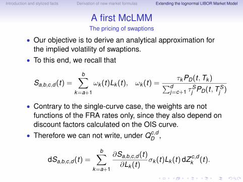
A first McLMMThe pricing of swaptions
• Our objective is to derive an analytical approximation forthe implied volatility of swaptions.
• To this end, we recall that
Sa,b,c,d(t) =b∑
k=a+1
ωk (t)Lk (t), ωk (t) =τkPD(t ,Tk )∑d
j=c+1 τSj PD(t ,T S
j )
• Contrary to the single-curve case, the weights are notfunctions of the FRA rates only, since they also depend ondiscount factors calculated on the OIS curve.
• Therefore we can not write, under Qc,dD ,
dSa,b,c,d(t) =b∑
k=a+1
∂Sa,b,c,d(t)∂Lk (t)
σk (t)Lk (t) dZ c,dk (t).

Introduction and stylized facts Derivation of new market formulas Extending the lognormal LIBOR Market Model
A first McLMMThe pricing of swaptions
• However, we can resort to a standard approximationtechnique and freeze weights ωk at their time-0 value:
Sa,b,c,d(t) ≈b∑
k=a+1
ωk (0)Lk (t),
thus also freezing the dependence of Sa,b,c,d on rates F Dh .
• Hence, we can write:
dSa,b,c,d(t) ≈b∑
k=a+1
ωk (0)σk (t)Lk (t) dZ c,dk (t).
• Like in the classic single-curve LMM, we then:• Match instantaneous quadratic variations• Freeze FRA and swap rates at their time-0 value

Introduction and stylized facts Derivation of new market formulas Extending the lognormal LIBOR Market Model
A first McLMMThe pricing of swaptions
• This immediately leads to the following (payer) swaptionprice at time 0:
PS(0,K ; Ta+1, . . . ,Tb,T Sc+1, . . . ,T
Sd )
=d∑
j=c+1
τSj PD(0,T S
j ) Bl(K ,Sa,b,c,d(0),Va,b,c,d
),
where the swaption volatility (multiplied by√
Ta) is given by
Va,b,c,d =
√√√√ b∑h,k=a+1
ωh(0)ωk (0)Lh(0)Lk (0)ρh,k
(Sa,b,c,d(0))2
∫ Ta
0σh(t)σk (t) dt
• Again, this formula is analogous in structure to thatobtained in the single-curve lognormal LMM.

Introduction and stylized facts Derivation of new market formulas Extending the lognormal LIBOR Market Model
A second McLMMA general framework for the single-tenor case
• Let us fix a given tenor x and consider a time structureT = {0 < T x
0 , . . . ,TxMx} compatible with x .
• Let us define forward OIS rates by
F xk (t) := FD(t ; T x
k−1,Txk ) =
1τ x
k
[PD(t ,T x
k−1)
PD(t ,T xk )
−1], k = 1, . . . ,Mx ,
where τ xk is the year fraction for the interval (T x
k−1,Txk ], and
basis spreads by
Sxk (t) := Lx
k (t)− F xk (t), k = 1, . . . ,Mx .
• By definition, both Lxk and F x
k are martingales under the
forward measure QT xk
D .
• Hence, their difference Sxk is a QT x
kD -martingale as well.
Introduction and stylized facts Derivation of new market formulas Extending the lognormal LIBOR Market Model
A second McLMMA general framework for the single-tenor case
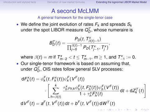
• We define the joint evolution of rates Fk and spreads Skunder the spot LIBOR measure QT
D , whose numeraire is
BTD (t) =PD(t ,T x
β(t)−1)∏β(t)−1j=0 PD(T x
j−1,Txj ),
where β(t) = m if T xm−2 < t ≤ T x
m−1, m ≥ 1, and T x−1 := 0.
• Our single-tenor framework is based on assuming that,under QT
D , OIS rates follow general SLV processes:
dF xk (t) = φF
k (t ,F xk (t))ψF
k (V F (t))
·
[k∑
h=β(t)
τ xh ρh,kφ
Fh (t ,F x
h (t))ψFh (V F (t))
1 + τ xh F x
h (t)dt + dZ Tk (t)
]dV F (t) = aF (t ,V F (t)) dt + bF (t ,V F (t)) dW T (t)
Introduction and stylized facts Derivation of new market formulas Extending the lognormal LIBOR Market Model
A second McLMMA general framework for the single-tenor case
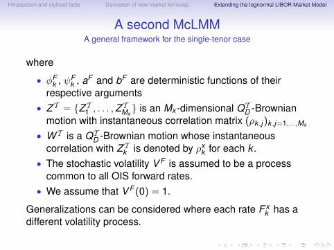
where
• φFk , ψF
k , aF and bF are deterministic functions of theirrespective arguments
• Z T = {Z T1 , . . . ,Z TMx} is an Mx -dimensional QT
D -Brownianmotion with instantaneous correlation matrix (ρk ,j)k ,j=1,...,Mx
• W T is a QTD -Brownian motion whose instantaneous
correlation with Z Tk is denoted by ρxk for each k .
• The stochastic volatility V F is assumed to be a processcommon to all OIS forward rates.
• We assume that V F (0) = 1.
Generalizations can be considered where each rate F xk has a
different volatility process.
Introduction and stylized facts Derivation of new market formulas Extending the lognormal LIBOR Market Model
A second McLMMA general framework for the single-tenor case
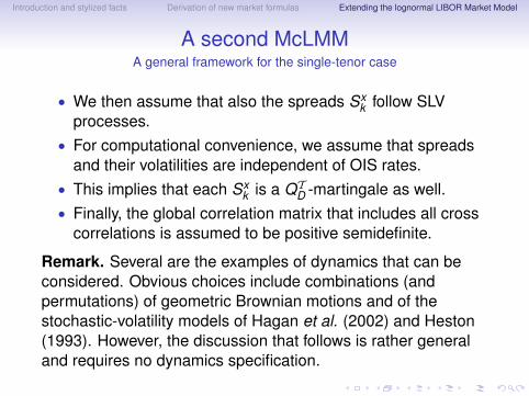
• We then assume that also the spreads Sxk follow SLV
processes.• For computational convenience, we assume that spreads
and their volatilities are independent of OIS rates.• This implies that each Sx
k is a QTD -martingale as well.
• Finally, the global correlation matrix that includes all crosscorrelations is assumed to be positive semidefinite.
Remark. Several are the examples of dynamics that can beconsidered. Obvious choices include combinations (andpermutations) of geometric Brownian motions and of thestochastic-volatility models of Hagan et al. (2002) and Heston(1993). However, the discussion that follows is rather generaland requires no dynamics specification.

Introduction and stylized facts Derivation of new market formulas Extending the lognormal LIBOR Market Model
A second McLMMCaplet pricing
• Let us consider the x-tenor caplet paying out at time T xk
τ xk [Lx
k (T xk−1)− K ]+
• Our assumptions on the discount curve imply that thecaplet price at time t is given by
Cplt(t ,K ; T xk−1,T
xk )
= τ xk PD(t ,T x
k )ET xk
D
{[Lx
k (T xk−1)− K ]+|Ft
}= τ x
k PD(t ,T xk )ET x
kD
{[F x
k (T xk−1) + Sx
k (T xk−1)− K ]+|Ft
}• Assume we explicitly know the QT x
kD -densities fSx
k (T xk−1)
andfF x
k (T xk−1)
(conditional on Ft ) of Sxk (T x
k−1) and F xk (T x
k−1),respectively, and/or the associated caplet prices.

Introduction and stylized facts Derivation of new market formulas Extending the lognormal LIBOR Market Model
A second McLMMCaplet pricing
• Thanks to the independence of the random variablesF x
k (T xk−1) and Sx
k (T xk−1) we equivalently have:
Cplt(t ,K ; T xk−1,T
xk )
τ xk PD(t ,T x
k )
=
∫ +∞
−∞ET x
kD
{[F x
k (T xk−1)− (K − z)]+|Ft
}fSx
k (T xk−1)
(z) dz
=
∫ +∞
−∞ET x
kD
{[Sx
k (T xk−1)− (K − z)]+|Ft
}fF x
k (T xk−1)
(z) dz
• One may use the first or the second formula depending onthe chosen dynamics for F x
k and Sxk .
• To calculate the caplet price one needs to derive thedynamics of F x
k and V F under the forward measure QT xk
D .• Notice that the QT x
kD -dynamics of Sx
k and its volatility are thesame as those under QT
D .

Introduction and stylized facts Derivation of new market formulas Extending the lognormal LIBOR Market Model
A second McLMMCaplet pricing
• The dynamics of F xk and V F under QT x
kD are given by:
dF xk (t) = φF
k (t ,F xk (t))ψF
k (V F (t)) dZ kk (t)
dV F (t) = aF (t ,V F (t)) dt + bF (t ,V F (t))
·
[−
k∑h=β(t)
τ xh φ
Fh (t ,F x
h (t))ψFh (V F (t))ρx
h1 + τ x
h F xh (t)
dt + dW k (t)
]
where Z kk and W k are QT x
kD -Brownian motions.
• By resorting to standard drift-freezing techniques, one canfind tractable approximations of V F for typical choices ofaF and bF , which will lead either to an explicit densityfF x
k (T xk−1)
or to an explicit option pricing formula (on F xk ).
• This, along with the assumed tractability of Sxk , will finally
allow the calculation of the caplet price.

Introduction and stylized facts Derivation of new market formulas Extending the lognormal LIBOR Market Model
A second McLMMSwaption pricing
• Let us consider a (payer) swaption, which gives the right toenter at time T x
a = T Sc an interest-rate swap with payment
times for the floating and fixed legs given by T xa+1, . . . ,T
xb
and T Sc+1, . . . ,T
Sd , respectively, with T x
b = T Sd and where
the fixed rate is K .• The swaption payoff at time T x
a = T Sc is given by
[Sa,b,c,d(T x
a )− K]+
d∑j=c+1
τSj PD(T S
c ,TSj ),
where the forward swap rate Sa,b,c,d(t) is given by
Sa,b,c,d(t) =
∑bk=a+1 τ
xk PD(t ,T x
k )Lxk (t)∑d
j=c+1 τSj PD(t ,T S
j ).

Introduction and stylized facts Derivation of new market formulas Extending the lognormal LIBOR Market Model
A second McLMMSwaption pricing
• The swaption payoff is conveniently priced under Qc,dD :
PS(t ,K ; T xa , . . . ,T
xb ,T
Sc+1, . . . ,T
Sd )
=d∑
j=c+1
τSj PD(t ,T S
j ) Ec,dD
{ [Sa,b,c,d(T x
a )− K]+ |Ft
}• To calculate the last expectation, we set
ωk (t) :=τ x
k PD(t ,T xk )∑d
j=c+1 τSj PD(t ,T S
j )and write:
Sa,b,c,d(t) =b∑
k=a+1
ωk (t)Lxk (t)
=b∑
k=a+1
ωk (t)F xk (t) +
b∑k=a+1
ωk (t)Sxk (t) =: F̄ (t) + S̄(t)
Introduction and stylized facts Derivation of new market formulas Extending the lognormal LIBOR Market Model
A second McLMMSwaption pricing
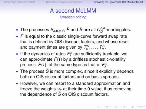
• The processes Sa,b,c,d , F̄ and S̄ are all Qc,dD -martingales.
• F̄ is equal to the classic single-curve forward swap ratethat is defined by OIS discount factors, and whose resetand payment times are given by T S
c , . . . ,T Sd .
• If the dynamics of rates F xk are sufficiently tractable, we
can approximate F̄ (t) by a driftless stochastic-volatilityprocess, F̃ (t), of the same type as that of F x
k .• The process S̄ is more complex, since it explicitly depends
both on OIS discount factors and on basis spreads.• However, we can resort to a standard approximation and
freeze the weights ωk at their time-0 value, thus removingthe dependence of S̄ on OIS discount factors.

Introduction and stylized facts Derivation of new market formulas Extending the lognormal LIBOR Market Model
A second McLMMSwaption pricing
• We then assume we can further approximate S̄ with adynamics S̃ similar to that of Sx
k , for instance by matchinginstantaneous variations.
• After the approximations just described, the swaption pricebecomes
PS(t ,K ; T xa , . . . ,T
xb ,T
Sc+1, . . . ,T
Sd )
=d∑
j=c+1
τSj PD(t ,T S
j ) Ec,dD
{[F̃ (T x
a ) + S̃(T xa )− K
]+|Ft}
which can be calculated exactly in the same fashion as theprevious caplet price.

Introduction and stylized facts Derivation of new market formulas Extending the lognormal LIBOR Market Model
A second McLMMA tractable class of multi-tenor models
• Let us consider a time structure T = {0 < T0, . . . ,TM} andtenors x1 < x2 < · · · < xn with associated time structuresT xi = {0 < T xi
0 , . . . ,TxiMxi}.
• We assume that each xi is a multiple of the precedingtenor xi−1, and that T xn ⊂ T xn−1 ⊂ · · · ⊂ T x1 = T .
• Forward OIS rates are defined, for each tenorx ∈ {x1, . . . , xn}, by
F xk (t) := FD(t ; T x
k−1,Txk ) =
1τ x
k
[PD(t ,T x
k−1)
PD(t ,T xk )
−1], k = 1, . . . ,Mx ,
and basis spreads are defined by
Sxk (t) = FRA(t ,T x
k−1,Txk )−F x
k (t) = Lxk (t)−F x
k (t), k = 1, . . . ,Mx .
• Lxk , F x
k , Sxk are martingales under the forward measure QT x
kD .

Introduction and stylized facts Derivation of new market formulas Extending the lognormal LIBOR Market Model
A second McLMMA tractable class of multi-tenor models
• We assume that, under the spot LIBOR measure QTD , the
OIS forward rates F x1k , k = 1, . . . ,M1, follow
“shifted-lognormal" stochastic-volatility processes
dF x1k (t) = σx1
k (t)V F (t)[ 1τ x1
k+ F x1
k (t)]
·
[V F (t)
k∑h=β(t)
ρh,kσx1h (t) dt + dZ Tk (t)
]dV F (t) = aF (t ,V F (t)) dt + bF (t ,V F (t)) dW T (t)
where:• For each k , σx1
k is a deterministic function;• {ZT
1 , . . . ,ZTM1} is an M1-dimensional QT
D -Brownian motionwith correlations (ρk,j)k,j=1,...,M1 ;
• V F is correlated with every ZTk , dW T (t)dZT
k (t) = ρxk dt , and
V F (0) = 1.

Introduction and stylized facts Derivation of new market formulas Extending the lognormal LIBOR Market Model
A tractable class of multi-tenor McLMMs• The dynamics of forward rates F x
k , for tenorsx ∈ {x2, . . . , xn}, can be obtained by Ito’s lemma, notingthat F x
k can be written in terms of “smaller” rates F x1k as
follows:
ik∏h=ik−1+1
[1 + τ x1h F x1
h (t)] = 1 + τ xk F x
k (t),
for some indices ik−1 and ik .• We then assume, for each tenor x ∈ {x1, . . . , xn}, the
following one-factor models for the spreads:
Sxk (t) = Sx
k (0)Mx(t), k = 1, . . . ,Mx ,
where, for each x , Mx is a (continuous and) positiveQT
D -martingale independent of rates F xk and of the
stochastic volatility V F . Clearly, Mx(0) = 1.

Introduction and stylized facts Derivation of new market formulas Extending the lognormal LIBOR Market Model
A tractable class of multi-tenor McLMMsRate dynamics under the associated forward measure
• When moving from measure QTD to measure QT x
kD , the drift
of a (continuous) process X changes according to
Drift(X ; QT xk
D ) = Drift(X ; QTD ) +
d〈X , ln(PD(·,T xk )/BTD (·))〉t
dt• Applying Ito’s lemma, we get, for each x ∈ {x1, . . . , xn},
dF xk (t) = σx
k (t)V F (t)[ 1τ x
k+ F x
k (t)]dZ k ,x
k (t)
where σxk , x ∈ {x2, . . . , xn}, is a deterministic function,
whose value is determined by σx1h and ρh,k , and
dV F (t) = −V F (t)bF (t ,V F (t))ik∑
h=β(t)
σx1h (t)ρx1
h dt
+ aF (t ,V F (t)) dt + bF (t ,V F (t)) dW k ,x(t)

Introduction and stylized facts Derivation of new market formulas Extending the lognormal LIBOR Market Model
A tractable class of multi-tenor McLMMs• The above dynamics of F x
k are the simplest stochasticvolatility dynamics that are consistent across differenttenors x .
• If 3m-rates follow shifted-lognormal processes withcommon stochastic volatility, the same type of dynamics(modulo the drift correction in the volatility) is also followedby 6m-rates (under the respective forward measures).
• This allows us to price simultaneously, with the same typeof formula, caps and swaptions with different tenors x .
• Option prices can then be calculated as suggested before.Swaption formulas can be simplified by noting that:
S̄(t) =b∑
k=a+1
ωk (t)Sxk (0)Mx(t)
≈Mx(t)b∑
k=a+1
ωk (0)Sxk (0) = S̄(0)Mx(t)

Introduction and stylized facts Derivation of new market formulas Extending the lognormal LIBOR Market Model
A tractable class of multi-tenor McLMMssAn explicit example of rate and spread dynamics
• We now assume constant volatilities σx1k (t) = σx1
k andSABR dynamics for V F . This leads to the followingdynamics for the x-tenor rate F x
k under QT xk
D :
dF xk (t) = σx
k V F (t)[ 1τ x
k+ F x
k (t)]dZ k ,x
k (t)
dV F (t) = −ε[V F (t)]2ik∑
h=β(t)
σx1h ρ
x1h dt + εV F (t) dW k ,x(t),
with V F (0) = 1, where also σxk is now constant and ε ∈ R+.
• We then assume that basis spreads for all tenors x aregoverned by the same geometric Brownian motion:
Mx ≡M, dM(t) = σM(t) dZ (t)
where Z is a QT xk
D -Brownian motion independent of Z k ,xk
and W k ,x and σ is a positive constant.
Introduction and stylized facts Derivation of new market formulas Extending the lognormal LIBOR Market Model
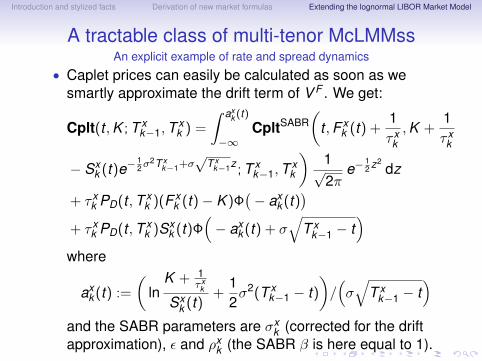
A tractable class of multi-tenor McLMMssAn explicit example of rate and spread dynamics
• Caplet prices can easily be calculated as soon as wesmartly approximate the drift term of V F . We get:
Cplt(t ,K ; T xk−1,T
xk ) =
∫ axk (t)
−∞CpltSABR
(t ,F x
k (t) +1τ x
k,K +
1τ x
k
− Sxk (t)e−
12 σ2T x
k−1+σ√
T xk−1z ; T x
k−1,Txk
)1√2π
e−12 z2
dz
+ τ xk PD(t ,T x
k )(F xk (t)− K )Φ
(− ax
k (t))
+ τ xk PD(t ,T x
k )Sxk (t)Φ
(− ax
k (t) + σ√
T xk−1 − t
)where
axk (t) :=
(ln
K + 1τ x
k
Sxk (t)
+12σ2(T x
k−1 − t))/(σ√
T xk−1 − t
)and the SABR parameters are σx
k (corrected for the driftapproximation), ε and ρx
k (the SABR β is here equal to 1).

Introduction and stylized facts Derivation of new market formulas Extending the lognormal LIBOR Market Model
A tractable class of multi-tenor McLMMssAn explicit example of rate and spread dynamics
• This caplet pricing formula can be used to price caps onany tenor x .
• In fact, cap prices on a non-standard tenor z can bederived by calibrating the market prices of standard y -tenorcaps using the formula with x = y and assuming a specificcorrelation structure ρi,j .
• One then obtains in output the model parameters:• σx1
k , k = 1, . . . ,M1• ρx1
k , k = 1, . . . ,M1• ε• σ
• Finally, with these calibrated parameters one can pricez-based caps, using again the caplet formula above, thistime setting x = z.

Introduction and stylized facts Derivation of new market formulas Extending the lognormal LIBOR Market Model
A tractable class of multi-tenor McLMMssAn explicit example of rate and spread dynamics
• We finally consider an example of calibration to marketdata of this multi-tenor McLMM.
• We use EUR data as of September 15th, 2010 andcalibrate 6-month caps with (semi-annual) maturities from3 to 10 years. The considered strikes range from 2% to 7%.
• We minimize the sum of squared relative differencesbetween model and market prices.
• We assume that OIS rates are perfectly correlated with oneanother, that all ρx1
k are equal to the same ρ and that thedrift of V F is approximately linear in V F .
• The average of the absolute values of these differences is19bp.
• After calibrating the model parameters to caps withx = 6m, we can apply the same model to price caps basedon the 3m-LIBOR (x = 3m), where we assume thatσ3m
ik−1= σ3m
ikfor each k .

Introduction and stylized facts Derivation of new market formulas Extending the lognormal LIBOR Market Model
A tractable class of multi-tenor McLMMssAn explicit example of rate and spread dynamics
Figure: Absolute differences (in%) between market and model capvolatilities.

Introduction and stylized facts Derivation of new market formulas Extending the lognormal LIBOR Market Model
A tractable class of multi-tenor McLMMssAn explicit example of rate and spread dynamics
Figure: Absolute differences (in bp) between model-implied3m-LIBOR cap volatilities and model 6m-LIBOR ones.

Introduction and stylized facts Derivation of new market formulas Extending the lognormal LIBOR Market Model
Conclusions• We started by describing the changes in market interest
rate quotes which have occurred since August 2007.• We have shown how to price the main interest rate
derivatives under the assumption of distinct curves forgenerating future LIBOR rates and for discounting.
• We have then shown how to extend the LMM to themulti-curve case, retaining the tractability of the classicsingle-curve LMM.
• We have finally introduced an extended LMM, where wejointly model rates and spreads with different tenors.
• References:• Mercurio, F. (2010a) Modern LIBOR Market Models: Using
Different Curves for Projecting Rates and for Discounting.International Journal of Theoretical and Applied Finance13, 1-25.
• Mercurio, F. (2010b) LIBOR Market Models with StochasticBasis. Available online on the ssrn web site.