Research Collection

Conference Paper

Full control of a quadrotor

Author(s): Bouabdallah, Samir; Siegwart, Roland Y.

Publication Date: 2007

Permanent Link: https://doi.org/10.3929/ethz-a-010039365

Originally published in: http://doi.org/10.1109/IROS.2007.4399042

Rights / License: In Copyright - Non-Commercial Use Permitted

This page was generated automatically upon download from the ETH Zurich Research Collection. For moreinformation please consult the Terms of use.

ETH Library

Full Control of a Quadrotor

Samir Bouabdallah and Roland SiegwartAutonomous Systems Lab

Swiss Federal Institute of Technology, ETHZZurich, Switzerland

samir.bouabdallah@ieee.org

rsiegwart@ethz.ch

Abstract— The research on autonomous miniature flyingrobots has intensified considerably thanks to the recent growthof civil and military interest in Unmanned Aerial Vehicles(UAV). This paper summarizes the final results of the modelingand control parts of OS4 project, which focused on designand control of a quadrotor. It introduces a simulation modelwhich takes into account the variation of the aerodynamicalcoefficients due to vehicle motion. The control parameters foundwith this model are successfully used on the helicopter withoutre-tuning. The last part of this paper describes the controlapproach (Integral Backstepping) and the scheme we proposefor full control of quadrotors (attitude, altitude and position).Finally, the results of autonomous take-off, hover, landing andcollision avoidance are presented.

I. INTRODUCTION

Flying objects have always exerted a great fascination onman encouraging all kinds of research and development.This project started in 2003, a time at which the roboticscommunity was showing a growing interest in UnmannedAerial Vehicles (UAV) development. The scientific challengein UAV design and control in cluttered environments and thelack of existing solutions was very motivating. On the otherhand, the broad field of applications in both military andcivilian markets was encouraging the funding of UAV relatedprojects. It was decided from the beginning of this projectto work on a particular configuration: the quadrotor. Theinterest comes not only from its dynamics, which representan attractive control problem, but also from the design issue.Integrating the sensors, actuators and intelligence into alightweight vertically flying system with a decent operationtime is not trivial.

A. State of the Art

The state of the art in quadrotor control has drasticallychanged in the last few years. The number of projects tack-ling this problem has considerably and suddenly increased.Most of these projects are based on commercially availabletoys like the Draganflyer [1], modified afterwards to havemore sensory and communication capabilities. Only fewgroups have tackled the MFR design problem. The thesis [2]lists some of the most important quadrotor projects of the last10 years. Mesicopter project [3], started in 1999 and endedin 2001. It aimed to study the feasibility of a centimeterscale quadrotor. E. Altug presented in his thesis a dualcamera visual feedback control [4] in 2003. The group of

Fig. 1. OS4 coordinate system.

Prof. Lozano has also a strong activity on quadrotors designand control [5]. N. Guenard from CEA (France) is also work-ing on autonomous control of indoor quadrotors [6]. Starmac,another interesting project, it targets the demonstration ofmulti agent control of quadrotors of about 1 kg.

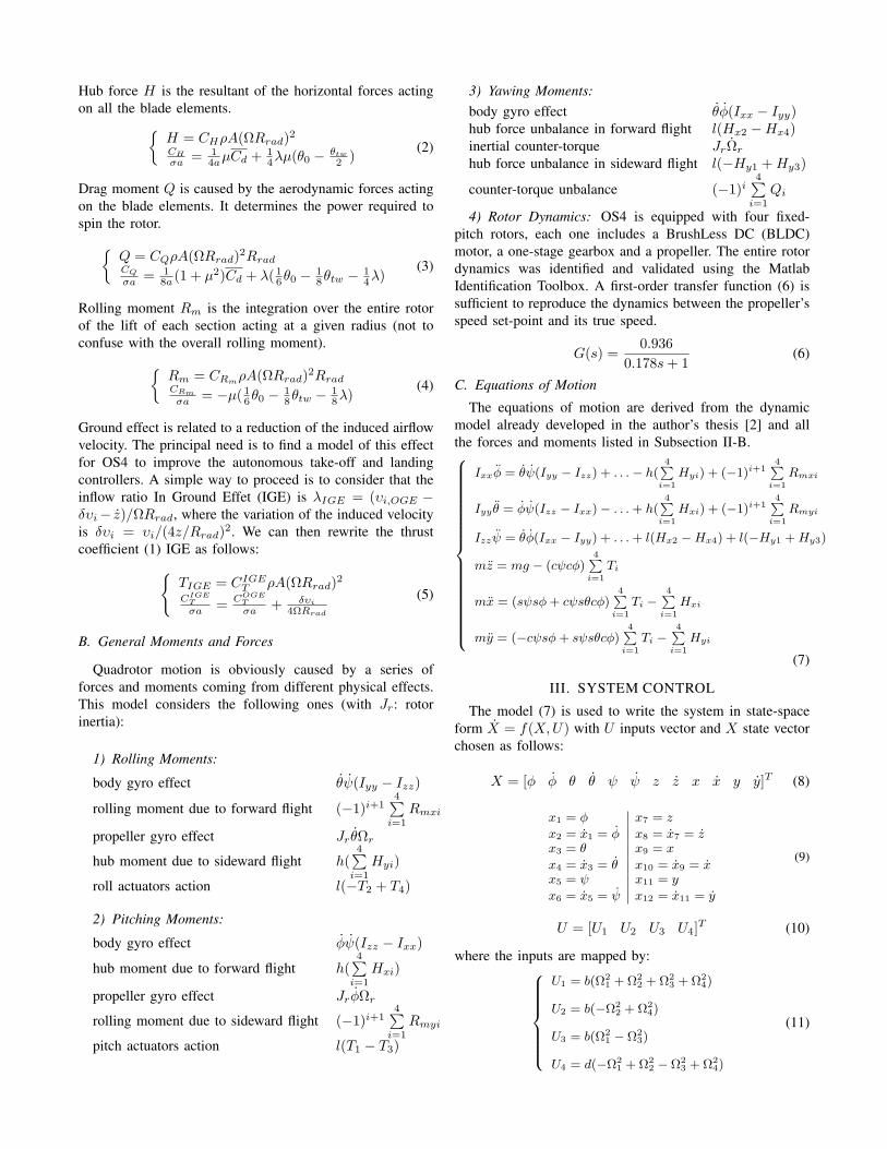
II. SYSTEM MODELINGThis simulation model was developed through some suc-

cessive steps as presented in papers [7], [8]. This last versionincludes hub forces H , rolling moments Rm and variableaerodynamical coefficients. This makes the model morerealistic particularly in forward flight. This section presentsthe model used for the last version of the OS4 simulatorwith which the Integral Backstepping (IB) controller wasdeveloped. The simulated control parameters were directlyused on the real helicopter for successful autonomous flights.Let us consider earth-fixed frame E and a body-fixed frameB as seen in Fig. 1. Using Euler angles parametrization, theairframe orientation in space is given by a rotation R fromB to E, where R ∈ SO3 is the rotation matrix.

A. Aerodynamic Forces and MomentsThe aerodynamic forces and moments are derived using

a combination of momentum and blade element theory [9].This is based on the work of Gary Fay in Mesicopter project[3]. For an easier reading of the equations below, we recallsome symbols. σ: solidity ratio, a: lift slope, µ: advance ratio,λ: inflow ratio, υ: induced velocity, ρ: air density, Rrad: rotorradius, l: distance propeller axis-CoG, θ0: pitch of incidence,θtw: twist pitch, Cd: drag coefficient at 70% radial station.See [2] for numerical values. Thrust force T is the resultantof the vertical forces acting on all the blade elements.

T = CT ρA(ΩRrad)2CT

σa = (16 + 1

4µ2)θ0 − (1 + µ2) θtw

8 − 14λ

(1)

Hub force H is the resultant of the horizontal forces actingon all the blade elements.

H = CHρA(ΩRrad)2CH

σa = 14aµCd + 1

4λµ(θ0 − θtw

2 )(2)

Drag moment Q is caused by the aerodynamic forces actingon the blade elements. It determines the power required tospin the rotor.

Q = CQρA(ΩRrad)2RradCQ

σa = 18a (1 + µ2)Cd + λ( 1

6θ0 −18θtw − 1

4λ)(3)

Rolling moment Rm is the integration over the entire rotorof the lift of each section acting at a given radius (not toconfuse with the overall rolling moment).

Rm = CRmρA(ΩRrad)2RradCRm

σa = −µ( 16θ0 −

18θtw − 1

8λ)(4)

Ground effect is related to a reduction of the induced airflowvelocity. The principal need is to find a model of this effectfor OS4 to improve the autonomous take-off and landingcontrollers. A simple way to proceed is to consider that theinflow ratio In Ground Effet (IGE) is λIGE = (υi,OGE −δυi− z)/ΩRrad, where the variation of the induced velocityis δυi = υi/(4z/Rrad)2. We can then rewrite the thrustcoefficient (1) IGE as follows:

TIGE = CIGET ρA(ΩRrad)2

CIGET

σa = COGET

σa + δυi

4ΩRrad

(5)

B. General Moments and Forces

Quadrotor motion is obviously caused by a series offorces and moments coming from different physical effects.This model considers the following ones (with Jr: rotorinertia):

1) Rolling Moments:

body gyro effect θψ(Iyy − Izz)

rolling moment due to forward flight (−1)i+14∑

i=1

Rmxi

propeller gyro effect Jr θΩr

hub moment due to sideward flight h(4∑

i=1

Hyi)

roll actuators action l(−T2 + T4)

2) Pitching Moments:

body gyro effect φψ(Izz − Ixx)

hub moment due to forward flight h(4∑

i=1

Hxi)

propeller gyro effect JrφΩr

rolling moment due to sideward flight (−1)i+14∑

i=1

Rmyi

pitch actuators action l(T1 − T3)

3) Yawing Moments:body gyro effect θφ(Ixx − Iyy)hub force unbalance in forward flight l(Hx2 −Hx4)inertial counter-torque JrΩr

hub force unbalance in sideward flight l(−Hy1 +Hy3)

counter-torque unbalance (−1)i4∑

i=1

Qi

4) Rotor Dynamics: OS4 is equipped with four fixed-pitch rotors, each one includes a BrushLess DC (BLDC)motor, a one-stage gearbox and a propeller. The entire rotordynamics was identified and validated using the MatlabIdentification Toolbox. A first-order transfer function (6) issufficient to reproduce the dynamics between the propeller’sspeed set-point and its true speed.

G(s) =0.936

0.178s+ 1(6)

C. Equations of Motion

The equations of motion are derived from the dynamicmodel already developed in the author’s thesis [2] and allthe forces and moments listed in Subsection II-B.

Ixxφ = θψ(Iyy − Izz) + . . .− h(4∑

i=1

Hyi) + (−1)i+14∑

i=1

Rmxi

Iyy θ = φψ(Izz − Ixx)− . . .+ h(4∑

i=1

Hxi) + (−1)i+14∑

i=1

Rmyi

Izzψ = θφ(Ixx − Iyy) + . . .+ l(Hx2 −Hx4) + l(−Hy1 +Hy3)

mz = mg − (cψcφ)4∑

i=1

Ti

mx = (sψsφ+ cψsθcφ)4∑

i=1

Ti −4∑

i=1

Hxi

my = (−cψsφ+ sψsθcφ)4∑

i=1

Ti −4∑

i=1

Hyi

(7)

III. SYSTEM CONTROL

The model (7) is used to write the system in state-spaceform X = f(X,U) with U inputs vector and X state vectorchosen as follows:

X = [φ φ θ θ ψ ψ z z x x y y]T (8)

x1 = φ x7 = z

x2 = x1 = φ x8 = x7 = zx3 = θ x9 = x

x4 = x3 = θ x10 = x9 = xx5 = ψ x11 = y

x6 = x5 = ψ x12 = x11 = y

(9)

U = [U1 U2 U3 U4]T (10)

where the inputs are mapped by:

U1 = b(Ω21 + Ω2

2 + Ω23 + Ω2

4)

U2 = b(−Ω22 + Ω2

4)

U3 = b(Ω21 − Ω2

3)

U4 = d(−Ω21 + Ω2

2 − Ω23 + Ω2

4)

(11)

With b thrust coefficient and d drag coefficient. The transfor-mation matrix between the rate of change of the orientationangles (φ, θ, ψ) and the body angular velocities (p, q, r) canbe considered as unity matrix if the perturbations from hoverflight are small. Then, one can write (φ, θ, ψ) ≈ (p, q, r).Simulation tests have shown that this assumption is reason-able. From (7), (8) and (10) we obtain after simplification:

f(X,U) =

φ

θψa1 + θa2Ωr + b1U2

θ

φψa3 − φa4Ωr + b2U3

ψ

θφa5 + b3U4

zg − (cosφ cos θ) 1

mU1

xux

1mU1

yuy

1mU1

(12)

With:a1 = (Iyy − Izz)/Ixx b1 = l/Ixx

a2 = Jr/Ixx b2 = l/Iyy

a3 = (Izz − Ixx)/Iyy b3 = 1/Izz

a4 = Jr/Iyy

a5 = (Ixx − Iyy)/Izz

(13)

ux = (cosφ sin θ cosψ + sinφ sinψ)uy = (cosφ sin θ sinψ − sinφ cosψ)

(14)

It is worthwhile to note in the latter system that the anglesand their time derivatives do not depend on translationcomponents. On the other hand, the translations dependon the angles. One can ideally imagine the overall systemdescribed by (12) as constituted of two subsystems, theangular rotations and the linear translations.

A. Control Approach Selection

During the OS4 project we explored several control ap-proaches from theoretical development to final experiments.As a first attempt, we tested on OS4 two linear controllers,a PID and an LQR based on a simplified model. The mainresult was an autonomous hover flight presented in [7]. How-ever, strong disturbances were poorly rejected as in presenceof wind. In the second attempt we reinforced the controlusing backstepping techniques. This time, we were able toelegantly reject strong disturbances but the stabilization inhover flight was delicate (see [8]). Another improvement isnow introduced thanks to integral backstepping (IB) [10].The idea of using integral action in the backstepping designwas first proposed in [11] and applied in [12] from whichthis control design was derived. After the evaluation ofall the control approaches tested in this work, it becameclear that the way to follow is a combination between PIDand Backstepping into the so-called Integral Backstepping.In fact, the backstepping is well suited for the cascadedstructure of the quadrotor dynamics. Moreover, the controllerdesign process can be straight forward if done properly. Inaddition, this method guarantees asymptotic stability and hasrobustness to some uncertainties, while the integral actioncancels the steady state errors. After a phase of extensive

IMU

Motor Speed

Control

Quadrotor

Vision sys. 1x Sonar4x Sonar

Obs. Avoid.

Control

Attitude

Control

Position

Control

Altitude

Control

Take-off/Landing

Control

Zd

Z

T

T

x,yx1,...,4

d

d1d

d

d_oa

d_oa

. . .

d

integral backstepping

PI

integral backstepping integral backstepping

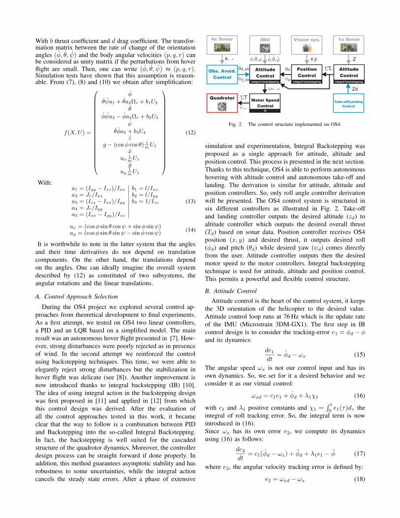
Fig. 2. The control structure implemented on OS4.

simulation and experimentation, Integral Backstepping wasproposed as a single approach for attitude, altitude andposition control. This process is presented in the next section.Thanks to this technique, OS4 is able to perform autonomoushovering with altitude control and autonomous take-off andlanding. The derivation is similar for attitude, altitude andposition controllers. So, only roll angle controller derivationwill be presented. The OS4 control system is structured insix different controllers as illustrated in Fig. 2. Take-offand landing controller outputs the desired altitude (zd) toaltitude controller which outputs the desired overall thrust(Td) based on sonar data. Position controller receives OS4position (x, y) and desired thrust, it outputs desired roll(φd) and pitch (θd) while desired yaw (ψd) comes directlyfrom the user. Attitude controller outputs then the desiredmotor speed to the motor controllers. Integral backsteppingtechnique is used for attitude, altitude and position control.This permits a powerful and flexible control structure.

B. Attitude Control

Attitude control is the heart of the control system, it keepsthe 3D orientation of the helicopter to the desired value.Attitude control loop runs at 76 Hz which is the update rateof the IMU (Microstrain 3DM-GX1). The first step in IBcontrol design is to consider the tracking-error e1 = φd − φand its dynamics:

de1dt

= φd − ωx (15)

The angular speed ωx is not our control input and has itsown dynamics. So, we set for it a desired behavior and weconsider it as our virtual control:

ωxd = c1e1 + φd + λ1χ1 (16)

with c1 and λ1 positive constants and χ1 =∫ t

0e1(τ)dτ the

integral of roll tracking error. So, the integral term is nowintroduced in (16).Since ωx has its own error e2, we compute its dynamicsusing (16) as follows:

de2dt

= c1(φd − ωx) + φd + λ1e1 − φ (17)

where e2, the angular velocity tracking error is defined by:

e2 = ωxd − ωx (18)

Using (16) and (18) we rewrite roll tracking error dynamicsas:

de1dt

= −c1e1 − λχ1 + e2 (19)

By replacing φ in (17) by its corresponding expression frommodel (12), the control input U2 appears in (20):

de2dt

= c1(φd−ωx)+φd+λ1e1−θψa1−θa2Ωr−b1U2 (20)

The real control input has appeared in (20). So, usingequations (15), (19) and (20) we combine the tracking errorsof the position e1, of the angular speed e2 and of the integralposition tracking error χ1 to obtain:

de2dt

= c1(−c1e1 − λ1χ1 + e2) + φd + λ1e1 − τx/Ixx (21)

where τx is the overall rolling torque. The desirable dynamicsfor the angular speed tracking error is:

de2dt

= −c2e2 − e1 (22)

This is obtained if one chooses the control input U2 as:

U2 = +1

b1[(1− c21 + λ1)e1 + (c1 + c2)e2

−c1λ1χ1 + φd − θψa1 − θa2Ωr] (23)

where c2 is a positive constant which determines theconvergence speed of the angular speed loop. Similarly, pitchand yaw controls are:

U3 = +1

b2[(1− c23 + λ2)e3 + (c3 + c4)e4

−c3λ2χ2 + θd − φψa3 + φa4Ωr] (24)

U4 = +1

b3[(1− c25 + λ3)e5 + (c5 + c6)e6 − c5λ3χ3](25)

with (c3, c4, c5, c6, λ2, λ3) > 0, and (χ2, χ3) the integralposition tracking error of pitch and yaw angles respectively.

1) Results: Attitude control performance is of crucialimportance, it is directly linked to the performance of theactuators. OS4 is equipped with motors powerful enoughto avoid amplitude saturation. However, they suffer fromlow dynamics and thus from bandwidth saturation. Theexperiment shown in Fig. 4 is a free flight were attitudereferences are zero. One can see in Fig. 3 that roll and pitchplots show a bounded oscillation of 0.1 rad in amplitude.This oscillation is not perceptible in flight, nevertheless it isdue to the slow dynamics of OS4’s actuators coupled withthe differences between the four propulsion groups. Controlparameters were in this experiment C1 = 10.5, C2 = 2,C3 = 10, C4 = 2, C5 = 2, C6 = 2. These are really closeto the parameters used in simulation which highlights thequality of the model.

0 5 10 15 20 25 30-0.5

-0.4

-0.3

-0.2

-0.1

0

0.1

0.2

0.3

0.4

0.5Roll angle

Rol

l [ra

d]

Time [s]0 5 10 15 20 25 30

-0.5

-0.4

-0.3

-0.2

-0.1

0

0.1

0.2

0.3

0.4

0.5Pitch angle

Pitc

h [r

ad]

Time [s]

0 5 10 15 20 25 30-0.5

-0.4

-0.3

-0.2

-0.1

0

0.1

0.2

0.3

0.4

0.5Yaw angle

Yaw

[rad

]

Time [s]

Fig. 3. Experiment: Integral backstepping attitude controller has to maintainattitude angles to zero in flight. The helicopter is stabilized despite thenumerous disturbances due to yaw drift, sensors noise and unmodeledeffects.

Fig. 4. OS4 in hover. A training frame was added for safety.

C. Altitude Control

The altitude controller keeps the distance of the helicopterto the ground at a desired value. It is based on a sonar(Devantech SRF10) which gives the range to the closestobstacle at 15 Hz. On the control law side, altitude trackingerror is defined as (ground effect is neglected):

e7 = zd − z (26)

The speed tracking error is:

e8 = c7e7 + zd + λ4χ4 − z (27)

The control law is then:

U1 =m

cosφcosθ[g+(1−c27+λ4)e7+(c7+c8)e8−c7λ4χ4] (28)

where (c7, c8, λ4) are positive constants.1) Take-off and Landing: The autonomous take-off and

landing algorithm adapts the altitude reference zd to followthe dynamics of the quadrotor for taking-off or landing. Thedesired altitude reference is gradually reduced by a fixed stepk (k > 0) which depends on the vehicle dynamics and thedesired landing speed. Moreover, the fact that the controlloop is much faster than the vehicle dynamics, makes thelanding very smooth.

2) Results: Altitude control works surprisingly well de-spite all the limitations of the sonar. Figure 5 shows analtitude reference profile (green) followed by the simulatedcontroller (red) and the real controller (blue). The task was

0 5 10 15 20 25 300

0.1

0.2

0.3

0.4

0.5

0.6

0.7OS4 take-off, altitude control and landing

Alti

tude

[m]

Time [s]

altitude reference (zd)altitude (z)simulated altitude (zs)

Fig. 5. Autonomous take-off, altitude control and landing in simulationand in real flight.

to climb to 0.5m, hover and then land. Control parameterswhere C7 = 3.5, C8 = 1.5 in simulation and C7 = 4, C8 = 2in experiment. The slight deviation between simulation andreality in take-off and landing phases is inherited fromactuators’ dynamics where the model was slightly slowerin the raising edge, and slightly faster in the falling one.Take-off is performed in 2 s (0-0.5 m) and landing in 2.8 s(0.5-0 m). Altitude control has a maximum of 3 cm deviationfrom the reference.

D. Position Control

Position control keeps the helicopter over the desiredpoint. It is meant here the (x, y) horizontal position withregard to a starting point. Horizontal motion is achieved byorienting the thrust vector towards the desired direction ofmotion. This is done by rotating the vehicle itself in the caseof a quadrotor. In practice, one performs position control byrolling or pitching the helicopter in response to a deviationfrom the yd or xd references respectively. Thus, the positioncontroller outputs the attitude references φd and θd, whichare tracked by the attitude controller (see Fig. 2). The thrustvector orientation in the earth fixed frame is given by R, therotation matrix. Applying small angle approximation to Rgives:

R =

1 ψ θψ 1 −φ−θ φ 1

(29)

From (12) and using (29) one can simplify horizontal motiondynamics to [

mxmy

]=

[−θU1

φU1

](30)

The control law is then derived using IB technique. Positiontracking errors for x and y are defined as:

e9 = xd − xe11 = yd − y

(31)

Accordingly speed tracking errors are:e10 = c9e9 + xd + λ5χ5 − xe12 = c11e11 + yd + λ6χ6 − y

(32)

0 5 10 15 20 25 30-1

-0.8

-0.6

-0.4

-0.2

0

0.2

0.4

0.6

0.8

1x position

x [m

]

Time [s]0 5 10 15 20 25 30

-1

-0.8

-0.6

-0.4

-0.2

0

0.2

0.4

0.6

0.8

1y position

y [m

]

Time [s]

0 5 10 15 20 25 30-1

-0.8

-0.6

-0.4

-0.2

0

0.2

0.4

0.6

0.8

1x speed

dx [m

/s]

Time [s]0 5 10 15 20 25 30

-1

-0.8

-0.6

-0.4

-0.2

0

0.2

0.4

0.6

0.8

1y speed

dy [m

/s]

Time [s]

Fig. 6. Simulation: Integral backstepping position controller drives attitudecontroller in order to maintain the helicopter over a given point.

Fig. 7. Four way-points for a square trajectory tracked by OS4.

The control laws are then: Ux = mU1

[(1− c29 + λ5)e9 + (c9 + c10)e10 − c9λ5χ5]

Uy = − mU1

[(1− c211 + λ6)e11 + (c11 + c12)e12 − c11λ6χ6]

(33)where (c9, c10, c11, c12, λ5, λ6) are positive constants.

1) Results: The main result in position control was ob-tained in simulation. Fig. 2 shows how the different con-trollers are cascaded. In fact, only the attitude is drivenby the position, altitude controller is simply feeding themwith U1. Attitude and position loops run at 76 Hz and 25 Hzrespectively. This spectral separation is necessary to avoid aconflict between the two loops; it is often accompanied withgain reductions in the driving loop. Control parameters wereC9 = 2, C10 = 0.5, C11 = 2, C12 = 0.5 in the simulation ofFig. 6.

2) Way-points following: The planner block in the simu-lator defines the way-points and hence the trajectories OS4has to follow. The position of the next way-point is sentto position controller which directs the vehicle towards thegoal. A way-point is declared reached when the helicopterenters a sphere around this point. The radius of this sphere(0.1 m) is the maximum admitted error. Figure 7 shows asquare trajectory defined by four way-points. The task wasto climb to 1 m from the ground and then follow the fourway-points of a square of 2 m side. In order to track thesquare trajectory, the planner generates the (xd, yd) positionreferences, and consequently the position controller generates

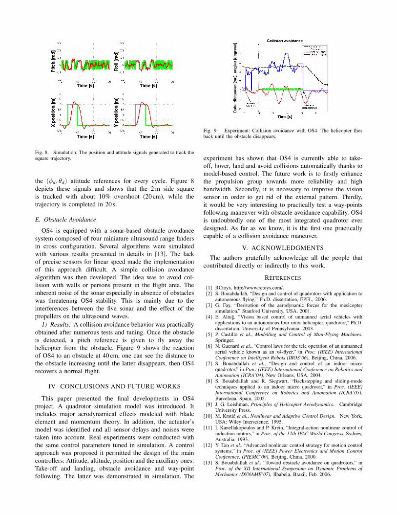
Fig. 8. Simulation: The position and attitude signals generated to track thesquare trajectory.

the (φd, θd) attitude references for every cycle. Figure 8depicts these signals and shows that the 2 m side squareis tracked with about 10% overshoot (20 cm), while thetrajectory is completed in 20 s.

E. Obstacle Avoidance

OS4 is equipped with a sonar-based obstacle avoidancesystem composed of four miniature ultrasound range findersin cross configuration. Several algorithms were simulatedwith various results presented in details in [13]. The lackof precise sensors for linear speed made the implementationof this approach difficult. A simple collision avoidancealgorithm was then developed. The idea was to avoid col-lision with walls or persons present in the flight area. Theinherent noise of the sonar especially in absence of obstacleswas threatening OS4 stability. This is mainly due to theinterferences between the five sonar and the effect of thepropellers on the ultrasound waves.

1) Results: A collision avoidance behavior was practicallyobtained after numerous tests and tuning. Once the obstacleis detected, a pitch reference is given to fly away thehelicopter from the obstacle. Figure 9 shows the reactionof OS4 to an obstacle at 40 cm, one can see the distance tothe obstacle increasing until the latter disappears, then OS4recovers a normal flight.

IV. CONCLUSIONS AND FUTURE WORKS

This paper presented the final developments in OS4project. A quadrotor simulation model was introduced. Itincludes major aerodynamical effects modeled with bladeelement and momentum theory. In addition, the actuator’smodel was identified and all sensor delays and noises weretaken into account. Real experiments were conducted withthe same control parameters tuned in simulation. A controlapproach was proposed it permitted the design of the maincontrollers: Attitude, altitude, position and the auxiliary ones:Take-off and landing, obstacle avoidance and way-pointfollowing. The latter was demonstrated in simulation. The

Fig. 9. Experiment: Collision avoidance with OS4. The helicopter fliesback until the obstacle disappears.

experiment has shown that OS4 is currently able to take-off, hover, land and avoid collisions automatically thanks tomodel-based control. The future work is to firstly enhancethe propulsion group towards more reliability and highbandwidth. Secondly, it is necessary to improve the visionsensor in order to get rid of the external pattern. Thirdly,it would be very interesting to practically test a way-pointsfollowing maneuver with obstacle avoidance capability. OS4is undoubtedly one of the most integrated quadrotor everdesigned. As far as we know, it is the first one practicallycapable of a collision avoidance maneuver.

V. ACKNOWLEDGMENTS

The authors gratefully acknowledge all the people thatcontributed directly or indirectly to this work.

REFERENCES

[1] RCtoys, http://www.rctoys.com/.[2] S. Bouabdallah, “Design and control of quadrotors with application to

autonomous flying,” Ph.D. dissertation, EPFL, 2006.[3] G. Fay, “Derivation of the aerodynamic forces for the mesicopter

simulation,” Stanford University, USA, 2001.[4] E. Altug, “Vision based control of unmanned aerial vehicles with

applications to an autonomous four rotor helicopter, quadrotor,” Ph.D.dissertation, University of Pennsylvania, 2003.

[5] P. Castillo et al., Modelling and Control of Mini-Flying Machines.Springer.

[6] N. Guenard et al., “Control laws for the tele operation of an unmannedaerial vehicle known as an x4-flyer,” in Proc. (IEEE) InternationalConference on Intelligent Robots (IROS’06), Beijing, China, 2006.

[7] S. Bouabdallah et al., “Design and control of an indoor microquadrotor,” in Proc. (IEEE) International Conference on Robotics andAutomation (ICRA’04), New Orleans, USA, 2004.

[8] S. Bouabdallah and R. Siegwart, “Backstepping and sliding-modetechniques applied to an indoor micro quadrotor,” in Proc. (IEEE)International Conference on Robotics and Automation (ICRA’05),Barcelona, Spain, 2005.

[9] J. G. Leishman, Principles of Helicopter Aerodynamics. CambridgeUniversity Press.

[10] M. Krstic et al., Nonlinear and Adaptive Control Design. New York,USA: Wiley Interscience, 1995.

[11] I. Kanellakopoulos and P. Krein, “Integral-action nonlinear control ofinduction motors,” in Proc. of the 12th IFAC World Congress, Sydney,Australia, 1993.

[12] Y. Tan et al., “Advanced nonlinear control strategy for motion controlsystems,” in Proc. of (IEEE) Power Electronics and Motion ControlConference, (PIEMC’00), Beijing, China, 2000.

[13] S. Bouabdallah et al., “Toward obstacle avoidance on quadrotors,” inProc. of the XII International Symposium on Dynamic Problems ofMechanics (DYNAME’07), Ilhabela, Brazil, Feb. 2006.