LiDAR Inpainting from a Single Image

Jacob Becker1, Charles Stewart1 and Richard J. Radke2∗

1Department of Computer Science2Department of Electrical, Computer, and Systems Engineering

Rensselaer Polytechnic Institute, Troy, NY USA 12180{beckej,stewart}@cs.rpi.edu, rjradke@ecse.rpi.edu

Figure 1. High-detail 3D structure is incrementally generated by our automatic image-guided LiDAR hole-filling algorithm.

AbstractRange scans produced by LiDAR (Light Detection and

Ranging) intrinsically suffer from “shadows” of missingdata cast on surfaces by occluding objects. In this paper, weshow how a single additional image of the scene from a dif-ferent perspective can be used to automatically fill in high-detail structure in these shadow regions. The techniqueis inspired by inpainting algorithms from the computer vi-sion literature, intelligently filling in missing informationby exploiting the observation that similar image regions of-ten correspond to similar 3D geometry. We first create anexample database of image patch/3D geometry pairs fromthe non-occluded parts of the LiDAR scan, describing eachuniform-scale region in 3D with a rotationally invariant im-age descriptor. We then iteratively select the best locationon the current shadow boundary based on the amount ofknown supporting geometry, filling in blocks of 3D geome-try using the best match from the example database and alocal 3D registration. We demonstrate that our algorithmcan generate realistic, high-detail new geometry in severalsynthetic and real-world examples.

1. IntroductionTime-of-flight LiDAR (Light Detection and Ranging)

scanners are capable of capturing highly accurate and de-tailed geometry of real-world objects. As a result, LiDARis increasingly used in surveying, architecture, cultural re-source management, archaeology, and other fields where

∗This work was supported in part by the DARPA Computer ScienceStudy Group under the award HR0011-07-1-0016.

accurate 3D models are useful. However, missing data inthe form of holes or “shadows” produced by occluding fore-ground surfaces are a common artifact of the scanning pro-cess.

In this paper, we show how a single additional imageof the scene from a different perspective can be used toautomatically fill in high-detail structure in these shadowregions. We first create an example database of imagepatch/3D geometry pairs from the non-occluded parts of theLiDAR scan, describing each uniform-scale region in 3Dwith a rotationally invariant image descriptor. We then iter-atively select the best location on the current shadow bound-ary based on the amount of known supporting geometry,filling in blocks of 3D geometry using the best match fromthe example database and a local 3D registration. Figure 1illustrates an example of our LiDAR inpainting algorithm,showing successive steps of high-detail hole filling.

The rest of the paper is organized as follows. In Section 2we review related work on filling holes in range data, withor without additional images. Section 3 defines the inputand output of the problem and describes data preprocessingsteps. Section 4 provides a taxonomy of holes that typicallyarise in LiDAR data. Section 5 describes our overall in-painting algorithm, including the generation of the exampledatabase, the definition of the patch fill order, and the fill-in algorithm itself. Section 6 presents experimental resultson both simulated and real datasets to demonstrate the tech-nique. Section 7 concludes the paper with discussion andideas for future work.

2. Related WorkThere has been a substantial amount of work on repair-

ing small to medium-sized holes in range data. For exam-ple, Stavrou et al. [16] adapted 2D image repair algorithmsto 3D data by treating the depth map of returns from thescanner as an image. Sharf et al. [15] proposed a hole-filing algorithm inspired by example-based image comple-tion methods. Using a volumetric descriptor, they searchedan example dataset for the closest match, and then warpedthe resulting geometry into the hole by solving a partial dif-ferential equation. Park et al. [13] extended the idea to workwith textured scans and solved the warping partial differen-tial equation in 2D.

Xu et al. [17] used a single image to guide hole-filling inrange data, by estimating normal vectors for points insidethe hole based on training data from image patches. Theyused the estimated normal vectors to integrate over the hole,producing 3D surfaces that were more physically accuratethan methods based purely on geometry, but tended to besmoother than the ground truth.

Techniques based on stereo [7, 6] and structure-from-motion [5, 1, 3] use multiple images to estimate 3D geom-etry. This geometry can be quite accurate, but is generallymuch sparser and more irregular than is typically acquiredwith a range scanner. Our interest in this paper is in learning3D structure from a single image/scan pair.

Hoiem et al. [11] used a supervised learning approach toclassify image superpixels into different geometric types,which were used to make realistic 3D “pop-ups” from asingle photograph. Saxena et al. [14] used a multi-scaleMarkov Random Field over superpixels in a supervisedlearning approach to generate 3D data from image patches.Neither approach can generate fine 3D geometric detail,which is our interest here.

Finally, Hessner and Basri [9] used a large database ofimage/depth pairs to estimate convincing depth informa-tion for images of people, hands, and fish. Our approachis related, but learns 3D structure in much larger-scale real-world architectural scans.

Our overall technique is inspired by recent work onexemplar-based image inpainting [4] and image analogies[10]. Criminisi et al. [4] presented an algorithm for auto-matically filling in a desired target area (e.g. a region tobe replaced in a digital photograph) with patches from asource region so that the resulting image seems unmanip-ulated. We adopt a similar idea of filling in LiDAR holesin a prioritized order depending on the amount of knowngeometry near a given pixel on the hole boundary. Hertz-mann et al. [10] automatically created image analogy filtersby transferring a learned relationship between a (originalimage, filtered image) pair to a new original image. Our al-gorithm uses a similar idea: we create a database of (imagepatch, 3D geometry) pairs from the non-hole regions of a

scan to estimate the 3D geometry that corresponds to a newimage patch.

3. Input, Output, and PreprocessingOur algorithm begins with a LiDAR scan S (Figure

2(a)), an image of the same scene from a different perspec-tive I (Figure 2(b)), and a camera model P that specifies theposition, orientation, and internal parameters of the cam-era that produced I in the coordinate system of S. In allthe real-world experiments reported here, we used a LeicaHDS3000 range scanner to obtain the scan S, which con-sists of a set of 3D points acquired using a 2D angular gridof rays from the scanner’s origin.

The camera model P could be found by manually select-ing correspondences between S and I and applying a resec-tioning algorithm [8], or automatically using a direct 2D-3Dregistration algorithm. For this paper, we used the direct al-gorithm proposed by Yang et al. [18], which is based on al-ternating between estimating the camera model from SIFTcorrespondences [12] and growing the region over whichthe estimated model is reliable. Figure 2(c) shows the resultof applying this algorithm to the scan/image pair in Figures2(a) and 2(b), re-rendering the LiDAR scan from the esti-mated perspective of the camera that acquired the image.

We run two preprocessing steps on the scan S. First, werobustly estimate the normal at each scan point by fitting alocal tangent plane, visiting relatively flat and noise-free re-gions first, since they are likely to produce stable estimates.We also create a simple quadrilateral mesh on S based onthe 2D grid of ray directions cast by the scanner, and iden-tify each edge in the grid as a surface edge or a boundarydiscontinuity based on the depth difference between adja-cent faces.

4. Types of HolesThree main types of holes generally exist in LiDAR

scans, as illustrated in Figure 3.

1. Occlusions (Figure 3 light gray lines). Since the clos-est surface to the scanner along each ray is what pro-duces the depth measurement, further scene pointsalong this ray on more distant surfaces appear as“shadows”. This is the most common type of hole.

2. No Returns (Figure 3 thick line). The laser pulse maynever return to the sensor for several reasons. For ex-ample, there may be no surface to reflect off of (i.e.,sky), the closest surface may be beyond the scanner’srange, or the surface material may be unconducive toscanning (e.g., windows and specular surfaces).

3. Out of View (Figure 3 medium gray lines). Scans witha finite angular extent have boundaries outside whichno geometry is acquired.

(a)

(b)

(c)

(d)

Figure 2. (a) A LiDAR scan S of an example environment. (b)An image I of the same environment from a different perspective.(c) A re-rendering of the LiDAR scan from the estimated perspec-tive of the camera that acquired the image in Figure 2(b). (d) Theinpainting mask M . Black corresponds to the source region andwhite to the target region to be inpainted.

Figure 3. Types of holes: occlusions (light gray), no returns(thick), and out of view (medium gray). Ray A is an example of afalse intersection. The solid black line is the scanned geometry.

For inpainting, we require a binary mask M that speci-fies which image pixels correspond to LiDAR holes. Gener-ally, these can be automatically identified by analyzing theno-geometry regions in the LiDAR scan re-rendered usingthe estimated camera model (i.e., black regions in Figure2(c)). Reasoning about which hole type corresponds to eachpixel is straightforward based on the view frustum of thecamera model and the boundary discontinuity informationgenerated at the preprocessing step; however, this classifi-cation is not strictly necessary for the inpainting algorithmproposed in the next section.

The non-hole regions of the image will be used to formthe source data for generating the example dataset of (im-age patch, 3D geometry) pairs. However, fully automaticgeneration of the source region from M is challenging dueto false intersections. That is, an optical ray in the imagemay intersect a surface close to the camera that did not pro-duce a LiDAR return, while the LiDAR scanner acquired3D geometry from a surface further along the optical ray(e.g., the ray labelled A in Figure 2(c)). While these pixelsare not LiDAR holes, they cannot be used for the inpaint-ing source region since the image texture and 3D geometryare inconsistent. While we explored several approaches toautomatically detect such regions (e.g., using image changedetection algorithms), we currently defer to the user to editthe mask M to ensure that false intersections are not in-cluded in the source region. Figure 2(d) illustrates the maskM for the scan/image pair in Figures 2(a)-2(c). We denotepixels where M=0 to be the source region (i.e., trusted im-age/geometry locations) and pixels where M=1 to be thetarget region to be filled by inpainting.

(a) (b) (c) (d)

Figure 4. (a) 3D point and surrounding area, (b) fitted planar patch with image samples and gradient, (c) head-on view of patch orientedwith dominant gradient direction up (top: high-resolution image used to estimate gradient, middle: corresponding 3D geometry, bottom:13×13 descriptor), (d) the mirrored patch that is also added to the database.

5. The Inpainting Algorithm

5.1. Generating the Example Database

Our first step is to generate an example database D ofimage patches and their corresponding 3D geometry. In thispaper, we use the source region defined by the mask M for agiven image to generate this database, although informationfrom other scan/image pairs (or multiple such pairs) couldalso be used. Since a fixed-size image region does not cor-respond to a fixed-size region in 3D space, we generate thedatabase using fixed-sized regions in 3D space, determinedby a user-defined radius r, and estimate rotation and scale-invariant image patch descriptors corresponding to a given3D region.

We iterate over each pixel i in I that is considered tobe trustworthy geometry in M (i.e., M(i) = 0). From thecamera model P , we know the corresponding intersectionwith the 3D scan S; denote this location S(i) (Figure 4(a)).We next fit a 3D planar patch Π to the set of LiDAR returnswithin a sphere of radius r centered at S(i), as illustrated inFigure 4(b). We impose a uniform grid on Π and estimate acolor at each grid point by projecting the planar patch intothe image using P and applying bilinear interpolation. Wereject patches that contain less than 90% trustworthy geom-etry (i.e., more than 90% of the patch must be outside a holeregion).

We now treat this colored planar patch as a small imageto be added to the example database. The descriptor weuse is simply a w2-length vector of pixel intensities corre-sponding to a subsampled w × w grid on Π (Figure 4(c)).The subsampled grid is oriented so that the x-axis is alignedwith the dominant gradient of the patch, estimated usingthe algorithm proposed by Lowe [12]. If multiple dominantgradients are detected (e.g., for a strong corner), we gener-ate multiple patch orientations and corresponding descrip-

tors. We also add a “mirror” of each patch to the databaseby reflecting it across its y-axis (Figure 4(d)), to make iteasier to find symmetries in the matching phase (see Sec-tion 5.3). Finally, we create a query kd-tree K from thedescriptors of all accepted patches, to ease the search prob-lem in the matching phase. Throughout this paper, we usedthe descriptor dimension w2 = 169, which we found toproduce good descriptive power while keeping the kd-treesearch fast.

5.2. Fill Order

The next step is to determine the fill order of pixels inthe target region. For image inpainting, Criminisi et al. [4]demonstrated that the order of filling in image patches hasa significant effect on the quality of the final result. Theirapproach defined the fill order based on a priority score thatwas the product of (1) a confidence term that measured theamount of known image texture surrounding a given pixelon the fill boundary and (2) a data term that was related tothe dot product between the normal vector to the fill regionboundary and the local image gradient. In our case, we onlyuse a confidence term since the auxiliary image providesgood visual evidence about how to fill the LiDAR hole (un-like image inpainting, where no side information about thehole interior is available).

Let b be a pixel on the boundary of the target region inM . As in Section 5.1, we fit a 3D planar patch Πb aroundthe 3D structure corresponding to pixel b, and backprojectthe values of M onto this plane to estimate the fraction ofthe patch that is part of the source region. If the patch isquantized with a grid of u × u bins, the confidence term isthus

C(b) =1u2

∑q∈Πb

M(q). (1)

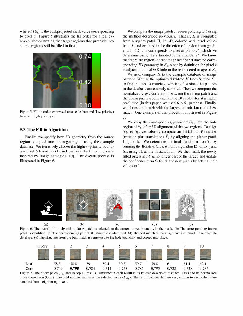
where M(q) is the backprojected mask value correspondingto pixel q. Figure 5 illustrates the fill order for a real ex-ample, demonstrating that target regions that protrude intosource regions will be filled in first.

Figure 5. Fill-in order, expressed on a scale from red (low priority)to green (high priority).

5.3. The Fill-in Algorithm

Finally, we specify how 3D geometry from the sourceregion is copied into the target region using the exampledatabase. We iteratively choose the highest-priority bound-ary pixel b based on (1) and perform the following stepsinspired by image analogies [10]. The overall process isillustrated in Figure 6.

We compute the image patch Ib corresponding to b usingthe method described previously. That is, Ib is computedfrom a square patch Πb in 3D, colored with pixel valuesfrom I , and oriented in the direction of the dominant gradi-ent. In 3D, this corresponds to a set of points Sb which wedetermine using the estimated camera model P . We knowthat there are regions of the image near b that have no corre-sponding 3D geometry in Sb, since by definition the pixel bis adjacent to a LiDAR hole in the re-rendered image of S.

We next compare Ib to the example database of imagepatches. We use the optimized kd-tree K from Section 5.1to find the top 10 matches, which is fast since the patchesin the database are coarsely sampled. Then we compute thenormalized cross-correlation between the image patch andthe planar patch around each of the 10 candidates at a higherresolution (in this paper, we used 61×61 patches). Finally,we choose the patch with the largest correlation as the bestmatch. One example of this process is illustrated in Figure7.

We copy the corresponding geometry Sdbinto the hole

region of Sb, after 3D alignment of the two regions. To alignSdb

to Sb, we robustly compute an initial transformation(rotation plus translation) Tb by aligning the planar patchΠdb

to Πb. We determine the final transformation Tb byrunning the Iterative Closest Point algorithm [2] on Sdb

andSb, using Tb as the initialization. We then mark the newlyfilled pixels in M as no longer part of the target, and updatethe confidence term C for all the new pixels by setting theirvalues to 1.

(a) (b) (c) (d) (e)Figure 6. The overall fill-in algorithm. (a) A patch is selected on the current target boundary in the mask. (b) The corresponding imagepatch is identified. (c) The corresponding partial 3D structure is identified. (d) The best match to the image patch is found in the exampledatabase. (e) The structure from the best match is registered to the hole boundary and copied into place.

Query 1 2 3 4 5 6 7 8 9 10

Dist 58.5 58.8 59.1 59.4 59.5 59.7 59.8 61 61.4 62.1Corr 0.749 0.795 0.784 0.741 0.753 0.785 0.795 0.733 0.738 0.736

Figure 7. The query patch (Ib) and its top 10 results. Underneath each result is its kd-tree descriptor distance (Dist) and its normalizedcross-correlation (Corr). The bold number indicates the selected patch (Ddb ). The result patches that are very similar to each other weresampled from neighboring pixels.

6. ExperimentsWe tested our algorithm on synthetic and real-world ex-

amples, with both artificially introduced and natural holes.All experiments were run on an 8-core 2.66GHz Xeon com-puter. For experiments where we have ground truth (Section6.1 and Section 6.2), we provide two quantitative measure-ments of the quality of the result. First, we compute themean Euclidean distance of from each filled in point pf tothe closest ground truth point pg , i.e., ‖pf−pg‖. The secondmeasure is the mean of the ratio

‖pf − Pc‖‖pg − Pc‖

(2)

where Pc is the location of the camera in the coordinate sys-tem of S. This measure is useful since it explicitly takesinto account the distance of from the sensors to the ac-quired/generated points.

6.1. 3D Letters

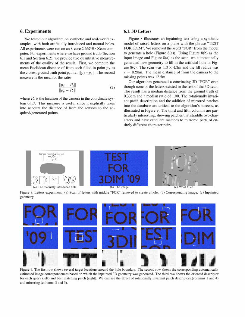
Figure 8 illustrates an inpainting test using a syntheticmodel of raised letters on a plane with the phrase “TESTFOR 3DIM”. We removed the word “FOR” from the modelto generate a hole (Figure 8(a)). Using Figure 8(b) as theinput image and Figure 8(a) as the scan, we automaticallygenerated new geometry to fill in the artificial hole in Fig-ure 8(c). The scan was 4.3 × 4.3m and the fill radius wasr = 0.20m. The mean distance of from the camera to themissing points was 12.5m.

Our algorithm generated a convincing 3D “FOR” eventhough none of the letters existed in the rest of the 3D scan.The result has a median distance from the ground truth of0.33cm and a median ratio of 1.00. The rotationally invari-ant patch description and the addition of mirrored patchesinto the database are critical to the algorithm’s success, asillustrated in Figure 9. The third and fifth columns are par-ticularly interesting, showing patches that straddle two char-acters and have excellent matches to mirrored parts of en-tirely different character pairs.

(a) The manually introduced hole (b) The image (c) Word filled

Figure 8. Letters experiment. (a) Scan of letters with middle “FOR” removed to create a hole. (b) Corresponding image. (c) Inpaintedgeometry.

Figure 9. The first row shows several target locations around the hole boundary. The second row shows the corresponding automaticallyestimated image correspondences based on which the inpainted 3D geometry was generated. The third row shows the oriented descriptorfor each query (left) and best matching patch (right). We can see the effect of rotationally invariant patch descriptors (columns 1 and 4)and mirroring (columns 3 and 5).

(a) Cropped view of the small win-dow

(b) Hole (c) Generated geometry (d) Original geometry

Figure 10. (a) Cropped view of the repetitive small windows. (b) One of the five windows is manually removed from the LiDAR scan. (c)Using the visual evidence from the image, new 3D structure is generated. (d) The original 3D structure for comparison.

(a) Example Image (b) Hole (c) Generated geometry

Figure 11. (a) Source image. (b) LiDAR scan. (c) Using the visual evidence from the image, new 3D structure is generated.

6.2. Small Window

We acquired a real scan of a large building with five sim-ilar windows near its roof (Figure 10(a)). We manually re-moved one of these small windows, so that no geometricevidence of the window remained (Figure 10(b)), and cre-ated the example database with with samples from the othersmall windows. For this experiment we set r = 0.35m.The mean distance from the camera to the scene points was72.4m. The filling algorithm took 52 iterations to completeand about 15min wall clock time; several snapshops of theiterations were shown in Figure 1. The final result is ren-dered in Figure 10(c), which compares favorably with theoriginal 3D geometry (Figure 10(d)) for the window. Themedian distance from the ground truth is 7.1cm, and themedian ratio is 1.00.

6.3. Large-scale LiDAR shadows

Finally, we ran our algorithm on several natural holesformed from occlusion in a real-world LiDAR scan, usingthe large church-like building in Figure 2. We note thatnot all of the holes have enough supporting evidence in thepatch/geometry database to be filled. Figure 11 illustrates aresult showing large swaths of filled-in texture. A closerview of one window is illustrated in Figure 12, showingconvincing high-detail 3D geometry.

7. Conclusions and Future WorkWe presented an algorithm for automatically filling in

convincing high-detail 3D structure in missing-data regions

(a) Original Model

(b) Filled Model

Figure 12. Detailed view of Figure 11 around the large window.

of a LiDAR scan using a single additional image of thescene from a different perspective. The approach can mit-igate the “shadows” characteristic of range scanning, im-proving the utility of LiDAR scans for planning and situ-ational awareness. Another application is the constructionof realistic architectural models; our algorithm works bestwhen repetitive structure is present, and this is quite oftenthe case with architecture. We note that while the generated

geometry is quite plausible, it should not be treated with thesame level of confidence as the real geometry.

The algorithm proposed here is only a first step to com-pletely solving the problem. We believe that a “data term”that uses partial 3D geometry to influence the fill orderand database matching is critical to improve the perceptualand actual quality of the results. We also plan to design amethod to determine when the inpainting is no longer reli-able or accurate, to prevent aggregating errors (e.g., whenextrapolating beyond the scan boundary). In this case, thehole type (occlusion, no return, out of view) should alsoplay a role in the fill priority and fill-in algorithms. Weare also investigating how to adaptively change the 3D in-painting radius based on estimated 3D structure (e.g., large,flat regions could be filled in more aggressively than small,complex regions). We also should consider how the descrip-tor dimension should vary with different scenes.

Finally, while the focus of this paper was on inpaintingfor a given target region, we also plan to automatically gen-erate the entire source and target regions, correctly detectingand discarding false intersections and reducing the amountof user input required to define these regions.

References[1] A. Abdelhafiz, B. Riedel, and W. Niemeier. Towards a 3d

true colored space by the fusion of laser scanner point cloudand digital photos. In Proc. of the ISPRS Working Group V/4Workshop (3D-ARCH), 2005.

[2] P. Besl and H. McKay. A method for registration of 3-dshapes. IEEE Trans. on Pattern Analysis and Machine In-telligence, 14(2):239–256, Feb. 1992.

[3] A. Brunton, S. Wuhrer, and C. Shu. Image-based modelcompletion. In Proc. of the 6th Int. Conf. on 3DIM, pages305–311, 2007.

[4] A. Criminisi, P. Perez, and K. Toyama. Region filling andobject removal by exemplar-based image inpainting. IEEETrans. Image Processing, 13:1200–1212, 2004.

[5] P. Dias, V. Sequeira, F. Vaz, and J. Goncalves. Registrationand fusion of intensity and range data for 3d modelling of

real world scenes. In Proc. 4th Int. Conf. on 3DIM, pages418–425, Oct. 2003.

[6] C. Frueh, S. Jain, and A. Zakhor. Data processing algorithmsfor generating textured 3d building facade meshes from laserscans and camera images. Int. J. Comp. Vis., 61(2):159–184,2005.

[7] C. Frueh, R. Sammon, and A. Zakhor. Automated texturemapping of 3d city models with oblique aerial imagery. InProc. 2nd Int. Symp. on 3DPVT, pages 396–403, Sept. 2004.

[8] R. I. Hartley and A. Zisserman. Multiple View Geometry inComputer Vision. Cambridge University Press, 2004.

[9] T. Hassner and R. Basri. Example based 3d reconstructionfrom single 2d images. In Proc. Beyond Patches Workshop,CVPR, pages 15–23, June 2006.

[10] A. Hertzmann, C. E. Jacobs, N. Oliver, B. Curless, and D. H.Salesin. Image analogies. In Proc. SIGGRAPH, pages 327–340, 2001.

[11] D. Hoiem, A. A. Efros, and M. Hebert. Automatic photopop-up. In ACM Trans. Graphics (SIGGRAPH ’05), August2005.

[12] D. G. Lowe. Distinctive image features from scale-invariantkeypoints. Int. J. Comp. Vis., 60(2):91–110, Nov. 2004.

[13] S. Park, X. Guo, H. Shin, and H. Qin. Shape and appearancerepair for incomplete point surfaces. In Proc. 10th ICCV,volume 2, pages 1260–1267, Oct. 2005.

[14] A. Saxena, S. H. Chung, and A. Y. Ng. 3-d depth reconstruc-tion from a single still image. Int. J. Comp. Vis., 76(1):53–69,Jan. 2008.

[15] A. Sharf, M. Alexa, and D. Cohen-Or. Context-based surfacecompletion. Proc. SIGGRAPH, 23(3):878–887, 2004.

[16] P. Stavrou, P. Mavridis, G. Papaioannou, G. Passalis, andT. Theoharis. 3d object repair using 2d algorithms. InProc. International Conference on Computational Science(2), pages 271–278, 2006.

[17] S. Xu, A. Georghiades, H. Rushmeier, J. Dorsey, andL. McMillan. Image guided geometry inference. In Proc.3rd Int. Symp. on 3DPVT, pages 310–317, 2006.

[18] G. Yang, J. Becker, and C. V. Stewart. Estimating the loca-tion of a camera with respect to a 3d model. In Proc. 6th Int.Conf. on 3DIM, pages 159–166, 2007.