Embed Size (px)
Citation preview
AVERTISSEMENT
Ce document est le fruit d'un long travail approuvé par le jury de soutenance et mis à disposition de l'ensemble de la communauté universitaire élargie. Il est soumis à la propriété intellectuelle de l'auteur. Ceci implique une obligation de citation et de référencement lors de l’utilisation de ce document. D'autre part, toute contrefaçon, plagiat, reproduction illicite encourt une poursuite pénale. Contact : [email protected]
LIENS Code de la Propriété Intellectuelle. articles L 122. 4 Code de la Propriété Intellectuelle. articles L 335.2- L 335.10 http://www.cfcopies.com/V2/leg/leg_droi.php http://www.culture.gouv.fr/culture/infos-pratiques/droits/protection.htm
UFR S.T.M.I.A. Département de Formation Doctorale en Mathématiques
École Doctorale IAE + M
Contribution à l'étude des processus stochastiques sur les -groupes quantiques
THÈSE
présentée et soutenue publiquement le 10 juin 1997
pour l'obtention du
Doctorat de l'Université Henri Poincaré - Nancy 1
(Spécialité Mathématiques)
par
Uwe FRANZ
Composition du jury
Président: Bernard ROYNETTE (Professeur à l'Université Henri Poincaré)
Rapporteurs: Luigi ACCARDI (Professeur à l'Université de Rome) Michael SCHÜRMANN (Professeur à l'Université Louis Pasteur, Strasbourg) Roland SPEICHER (Professeur à l'Université de Heidelberg)
Examinateurs: Heinz-Dietrich DOEBNER (Professeur à l'Université de Clausthal) Remi LEANDRE (Directeur de Recherches au CNRS, IECN, Université Henri Poincaré) René SCHOTT (Professeur à l'Université Henri Poincaré, directeur de la thèse) .
Institut de Mathématiques Élie Cartan de Nancy

Résumé
Ce mémoire est rélatif à l'étude des processus stochastiques sur les algèbres de Hopf. Ces algèbres jouent un rôle important en physique mathématique sous le nom groupes quantiques.
Une grande partie -de cette tlïèse est-consacrée à l'étude des processus de Lévy, c-àd des processus à accroissements indépendants et stationnaires, sur ces algèbres. Deux constructions, soit à partir d'un processus de Lévy classique, soit à partir d'une marche aléatoire quantique, sont proprosées. Ces processus sont ensuite étudiés à l'aide des représentations duales et de leurs systèmes d'Appell. En particulier, ceci a permis de démontrer une formule de Feynman-Kac et d'établir un lien étroit entre ces processus et des équations d'évolution sur les groupes quantiques.
Les représentations duales sont également utilisées pour donner des conditions suffisantes pour l'existence de versions classiques des processus de Lévy sur des bigèbres et pour les caractériser. Plusieurs exemples, y compris la martingale d'Azéma, sont traités en détail.
Un autre thème central de ce travail est la caractérisation des lois de Gauss au sens de Bernstein. Il est montré comment les fonctionnelles ainsi que les semi-groupes de convolution sur des algèbres de Hopf qui satisfont l'analogue de la propriété de Bernstein peuvent être calculés. Il est aussi démontré que le plongement d'une fonctionnelle normée infiniment divisible dans un semi-groupe de convolution continu sur un groupe quantique nilpotent ou sur un groupe tressé nilpotent est unique.
Finalement, plusieurs théorèmes limites (loi des grands nombres, théorème de la limite centrale, etc.) sur les groupes quantiques sont présentés.
Mots-clés: Processus de Lévy sur des bigèbres, théorèmes limites
Abstract
In this thesis stochastique processus on Hopf algebras are studied. These algebras, also known un der the name quantum group, play in important role in mathematical physics.
A major part of this workis concerned with Lévy processes, i.e. processes with stationary and independent increments. Two construction are proposed, one starts from a classical Lévy process, the other one uses quantom random walks. These pro cesses are then studied with the help of dual representations and Appell systems. This has allowed us to prove an analogue of the Feynman-Kac formula, and to study the relation between the pro cesses and their evolution equations.
Dual representations are also used to give sufficient conditions for the existence of classical versions of Lévy processes on bialgebras, and to calculate the classical generators. Several examples including the Azéma martingale are treated in detail.
Another central theme is the classification of Gaussian laws. It is shown, how the functionals and convolution semigroups that satisfy an analogue of the Bernstein property can be determined. 'vVe also prove the the embedding of a normalized functional into a continuous convolution semigroup on a nilpotent quantum group or nilpotent braided group lS umque.
Finally, there are also several limit theorems (law of large numbers, central limit theorem, etc.) presented in this work.
Mathematics Subject Classifications (1991): "'60B99 Probability theory on general structures, 16W30 Hopf algebras (assoc. rillgs and algebras), 60FO:) Weak limit theorems.

Remerciements
En premier lieu, je tiens à remercier Monsieur René Schott, Professeur à l'Université Henri Poincaré-Nancy 1, qui m'a suivi durant toute ma thèse. Il a investi énormément de temps et d'énergie pour me soutenir, discuter et me conseiller.
Je remercie également très vivement: Le Professeur Luigi Accardi de l'Université de Rome d'avoir accepté la charge de
rapporter le présent travail. J'ai apprécié son accueil à Frascati et l'intérêt qu'il a manifesté pour cette thèse.
Le Professeur Michael Schürmann de l'Université Louis Pasteur à Strasbourg d'avoir accepté d'écrire un rapport sur ce travail. J'ai particulièrement apprécié ses remarques et ses précieux conseils.
Le Professeur Roland Speicher de l'Université de Heidelberg d'avoir accepté le rôle de rapporteur. Je garde un très bon souvenir des discussions que nous avons eues.
Le Professeur Heinz-Dietrich Doebner de l'Université de Clausthal qui m'a suivi pas seulement pendant cette thèse mais durant toutes mes études universitaires.
Monsieur Remi Léandre, Directeur de Recherches au CNRS à l'IECN, Université Henri Poincaré-Nancy 1, d'avoir accepté de juger ce travail; nos discussions et sa curiosité scientifique m'ont beaucoup apporté.
Le Professeur Bernard Roynette de l'Université Henri Poincaré-Nancy 1 pour avoir accepté de présider le jury. Son accueil, sa convivialité et l'ambiance qu 'il a su instaurer au sein de l'équipe m'ont beaucoup aidé à travailler.
Je tiens aussi à remercier Philip Feinsilver, Professeur de Southern Illinois University - Carbondale, pour "making things happen," pour sa chaleureuse hospitalité lors de mon séjour à Carbondale et pour les innombrables discussions qu'on a partagées.
Je remercie également, pour leur aide, les membres de l'Institut Elie Cartan, de l'Equipe AMII et de l'ASI-TPA à Clausthal, ainsi que tous mes amis à Nancy et ailleurs.

IV

Avant-propos
Cette thèse se compose de cinq articles en anglais:
- Chapitre 4: Duality and Multiplicative Stochastic Pro cesses on Quantum Groups
- Chapitre 5: Diffusions on Braided Spaces
- Chapitre 6: Gauss Laws in the Sense of Bernstein and Uniqueness of Embedding into Convolution Semigroups on Quantum Groups and Braided Groups
- Chapitre 7: Evolution Equations and Lévy Processus on Quantum Groups
- Chapitre 8: Brownian Motion on the Affine Group and Generalized Gegenbauer Polynomials
et de deux chapitres sur des travaux en cours, également en anglais:
- Chapitre 9: Limit theOl'ems on Quantum Groups
- Chapitre 10 Classical Versions of Quantum Lévy Processes,
qui forment ensemble la deuxième partie. La première partie, composée de trois chapitres, est une synthèse en français des
résultats essentiels. Après l'introduction nous donnons un bref aperçu de la théorie des processus de Lévy sur les bigèbres. Ensuite, dans le Chapitre 3, les résultats propres à ce travail sont énoncés. Une bibliographie se trouve a la fin.
v

VI Avant-propos
Table des matières
Résumé
Abstract
1 Avant-propos
Partie 1 Synthèse
1 Introduction
2 Processus stochastiques sur des bigèbres
2.1 Probabilités non-commutatives
2.2 Bigèbres et algèbres de Hopf.
2.3 Catégories tressées
2.4 Indépendance...
2.5 Processus de Lévy sur les bigèbres
3 Les résultats principaux
3.1 Construction des processus de Lévy et des semi-groupes de convolution
1
3
5
5
6
9
12
13
15
sur les bigèbres . . . . . . . . . . . . . . . . . . . 15
3.2 Processus stochastiques et équations d'évolution. 16
3.3 Caractérisation . . . . . . . . . . . 17
3.4 Théorèmes limites sur les bigèbres. 18
3.5 Versions classiques des processus de Lévy quantiques 18
3.6 Recherche future . . 19
3.7 Liste de publications 20
VIl

Vlll Table des matières
Partie II 23
4 Duality and Multiplicative Stochastic Pro cesses on Quantum Groups 25
4.1 Introduction.
4.2 Preliminaries
4.3 q-Exponentials
4.4 Dual representations
4.5 Construction .,. .
4.6 Feynman-Kac formula
4.7 Appell systems ....
4.8 Extension of the construction
4.9 Conclusion
5 Diffusions on Braided Spaces
.5.1 Iutroduction.
5.2 Preliminaries
.5.2.1 Braided spaces
.5.2.2 Quantum probability and quantum Lévy processes
.5.2.:3 A remark on braided * -Hopf algebras . . . . . . .
5.:3 A construction of (pseudo-) diffusions on braided spaces
5.3.1 Examples of (pseudo-) diffusions
.5.3.2 Examples of true diffusions
5.4 Appell systems ........ .
5.4.1 The braided line IRq ..
5.4.2 The quantum plane (C~lo
5.4.3 The free braided-space
5.5 Densities..
5.6 Conclusion
6 Gauss Laws in the Sense of Bernstein on Quantum Groups
6.1 Introduction.
6.2 Preliminaries
6.2.1 Quantum groups
6.2.2 Quantum probability .
27
27
29
:32
:34
:35
:38
41
44
45
47
48
48
.50
.52
53
.56
58
60
62
62
63
63
64
67
69
69
69
70

6.3 A braided Heisenberg-'Weyl group ...... .
6.4 Gaussian functionals in the sense of Bernstein
6.4.1 Definition of Gaussian functionals in the sense of Bernstein on
(braided) Hopf algebras
6.4.2
6.4.3
6.4.4
6.4.5
6.4.6
6.4.7
6.4.8
Independence . . .
Preliminary results
The braided line .
The braided plane
The braided q-Heisenberg algebra .
Positivity
Remarks.
6.5 U niqueness of embedding
6.5.1 Definition of nilpotence
6.5.2
6.5.3
6.5.4
Poincaré-Birkhoff-Witt property and nilpotence
Uniqueness of embedding
Remark ......... .
6.6 Gaussian semigroups in the sense of Bernstein
6.6.1 Definition of Gaussian convolution semigroups in the sense of
Bernstein . . .
6.6.2
6.6.3
6.6.4
General results
The braided line
The braided plane
6.6.5 The braided q-Heisenberg-Weyl group
6.6.6 lRq-quantum convolution semigroups
6.7 Conclusion ................. .
IX
71
73
74
75
76
78
79
80
81
82
8:3
84 Q~
l/J
8.5
86
87
87
89
89
90
91
91
7 Evolution Equations and Lévy Pro cesses on Quantum Groups 93
7.1 Introduction. 95
7.2 Preliminaries 95
7.3 Evolution equations
7.4 Quantum stochastic pro cesses
7.5 Appell systems ....... .
7.5.1 Example: The braided li ne .
7.5.2 Example: The braided plane.
7.5.3 Example: The q-affine group.
98
98
99
99
100
100

x Table des matièr'es
7.5.4 Example: The braided q-Heisenberg-Weyl group
7.6 Densities .............. .
7.6.1 Example: The braided line .
7.6.2 Example: The braided plane.
7.6.3 Example: The q-affine group.
7.6.4 Example: The q-Heisenberg-YVeyl algebra
707 Conclusion 0>0 •• ___ •••••• _ •• .. •••• " • • • • " • ~ " o· •
101
102
103
104
104
105
105
8 Brownian Motion and Generalized Gegenbauer Polynomials 107
8.1 Introduction..............
8.2 Brownian motion on the affine group
8.3 Group elements and matrix elements
8.4 Multiplication rules and addition formulae
8.5 Orthogonality.
8.6 Appell Systems
9 Limit Theorems on Quantum Groups
9.1
9.2
Introduction .............. .
Analogues of the law of large numbers and the central limit theorem
9.2.1 General results for limit theorems on bialgebras
9.2.2 The braided line ........... .
9.2.3 The braided q-Heisenberg-Weyl group
9.3 Law of iterated logarithm type results
109
109
111
112
114
116
119
121
121
121
122
123
123
9.3.1 Definition of the supremum for quantum stochastic variables 123
9.3.2 Calculation of the distribution of sup Xl, ... ,Xn . 124
9.3.3 Calculation of the supremum of a Markov chain 126
9.3.4 Continuous time Emit . . . . . . . 127
9.4 A mixed classical-quantum limit theorem .
9.4.1 The algebra U .....
9.4.2 Proof of Theorem 9.4.1 .
9.5 Operator-limit theorems on bialgebras
10 Classical Markov Processes from Quantum Lévy Processes
10.1 Introduction .................. .
10.2 Classical versions of quantum Lévy pro cesses .
127
128
129
131
133
135
13,5
10.2.1 Quantum Lévy processes ......... .
10.2.2 From quantum Lévy to quantum Markov.
10.2.3 From quantum Markov to classical Markov.
10.3 Examples of classical versions of Lévy pro cesses on IRq * IRl/q
10.3.1 The Azéma martingale ....
10.3.2 Other processes on IRq * IRl/q.
Bibliographie
Index
Xl
135
135
136
137
138
1:39
143
151

Xll Table des matières
Première partie
Synthèse
1


Chapitre 1
Introduction
La manière dont les probabilités quantiques sont obtenues à partir des probabilités classiques ressemble, du moins formellement, à la transition de la mécanique classique à la mécanique quantique. Les observables, appelées variables aléatoires en théorie des probabilités, sont autorisées à vérifier des relations de commutation non triviales (i.e. l'algèbre commutative des fonctions mesurables sur un espace probabilisé est remplacée par une certaine (*-)algèbre non commutative).
Les groupes quantiques dérivent de façon analogue des groupes classiques. L'algèbre de Hopf abélienne des fonctions représentatives est remplaçée par une "déformation" non commutative. De la structure de groupe il reste la structure de cogèbre qui nous permet de définir la plupart des constructions de la théorie des groupes de façon plus générale pour des algèbres de Hopf ou bigèbres.
Le présent travail tente de combiner ces deux notions. Nous étudions des processus quantiques sur des groupes quantiques. Ces processus sont les analogues non-commutatifs naturels des processus stochastiques à valeurs dans les groupes. Nous sommes donc particulièrement interessés par les propriétés qui utilisent la structure de cogèbre, par exemple la théorie des processus à accroissements indépendants et stationnaires (les processus de Lévy), où la notion d'accroissement est maintenant définie via le coproduit au lieu de la loi du groupe. Nous nous sommes aussi intéressés aux théorèmes limites et à la caractérisation de certaines lois de probabilité également basées sur le coproduit.
Nous faisons à présent un bref survol des résultats contenus dans cette thèse, les définitions exactes et les formulations précises sont données aux chapitres 2 et 3.
Les thèmes centraux sont:
- la construction des processus de Lévy et de leurs semi-groupes de convolution sur les bigébres,
- le lien entre les processus de Lévy et les équations d'évolution,
- étude des versions classiques des processus de Lévy sur les bigébres,
- la caractérisation de certaines classes de fonctionnelles a l'aide de leurs propriétés par rapport à la structure de cogèbre,
- des théorèmes limites, avec caractérisation des lois limites.
3

4 Chapitre 1. Introduction
La première partie est un sommaire. Le chapitre 2 contient toutes les définitions de base et tous les résultats dont nous aurons besoin par la suite.
Les résultats essentiels sont énoncés au chapitre 3. A la fin de ce chapitre nous avons inclus une liste des publications auxquelles cette
thèse a donné lieu (voir section 3.7, page 20).

Chapitre 2
Processus stochastiquès sur des bigèbres
Ce chapitre présente une brève introduction à la théorie des processus stochastiques sur des bigèbres, basée essentiellement sur le livre de M. Schürmann[Sch93].
La notion d'indépendance tensorielle à gauche ou à droite est généralisée à l'indépendance tressée.
2.1 Probabilités non-commutatives
Nous résumons les définitions les plus importantes concernant les probabilités quantiques ou non-commutatives, pour une introduction plus détaillée on pourra consulter, par exemple, les livres de Biane [Bia93], de Meyer [Mey93], et de Parthasarathy [Par92].
Un espace de probabilité non-commutatif (quantum probability space) est un couple (A, <p) où A est une algèbre involutive sur œ et <P un état (state) sur A, càd une fonctionnelle linéaire positive normalisée. Un espace de probabilité classique définit un espace de probabilité non-commutatif si on prend une algèbre convenable de fonctions intégrables à valeurs complexes sur !1, par exemple LOO(!1, F, P), et la fonctionnelle <P : f H- In fdP.
Une variable aléatoire non-commutative (quantum random variable) j sur un espace de probabilité non-commutatif (A, <p) est un homomorphisme de *-algèbre j : B -t A. À partir d'une variable aléatoire classique à valeurs dans un espace mesurable (E, E) on peut définir une variable aléatoire non-commutative en posant jx(J) = foX pour f E B (où l'algèbre B des fonctions mesurables sur (E, E) est choisie t.q. foX E A). La fonctionnelle !.pj = <P 0 j est appelée la distribution de j dans l'état <P.
Un processus stochastique non-commutatif ( quantum stochastic process) n'est rien d'autre qu'une famille de variables aléatoires {jt; t E I} sur le même espace de probabilité noncommutatif, indexée par un ensemble l, comme dans le cas classique. Ses distributions uni-dimensionnelles (one-dimensional ou marginal distributions) sont les fonctionnelles !.pt = <P 0 jt.
Deux processus stochastiques non-commutatifs {jt : B -t (Aj, <Pj); tE I} et {kt: B -t
(Ak, <Pk); tEl}, indexés par le même ensemble l, définis sur la même algèbre B, sont
5

6 Chapitre 2. Processus stochastiques SUl' des bigèbres
équivalents, si <I> j (jtl (b l ) •.. jtn (bn )) = <I> k ( ktl (b l ) ... ktn (bn ) ) ,
pour tous n E IN, t l , ... ,in E I, bl , ... , bn E B. Un élément a d'un espace de probabilité non-commutatif définit une variable aléa
toire sur Œ < z,z* > (= l'algèbre libre engendrée par z,z*), ou sur Œ[z] (= l'algèbre des polynômes à valeurs complexes sur IR), si a est auto-adjoint. On prend simplement l'homomorphisme de *-algèbre défini par j(z) = a. De la même façon toute famille {at; i E I} d'éléments de A devient un processus stochastique non-commutatif indexé par I.
Ceci permet d'associer une densité sur la droite· réelle à un élément auto-adjoint a d'un espace de probabilité non-commutatif. Une densité de a (dans l'état <I» est une mesure f1 sur IR telle que <I>(a n ) = JlRxndf1(x) pour tout ri E IN. Cette mesure n'est pas nécessairement unique. Une variable aléatoire X sur un espace de probabilité (D, F, P) à valeurs dans IR est une version classique de a si sa loi Px est une densité de a. Pour la version classique f\t; t E I} d'un processus stochastique non-commutatif on demande seulement que les moments ordonnés coïncident, c-à-d
2.2 Bigèbres et algèbres de Hopf
Les textes classiques sur les algèbres de Hopf sont [Swe69, Abe80], mais voir aussi [DHL91, SS9:3, CP95, Gui95, Kas95, Maj95b].
Une algèbre associative A sur un corps lK est un lK-espace vectoriel muni d'une application linéaire m : A 0 A -+ A telle que
m 0 (m 0 id) = m 0 (id 0 m) ( associati vi ty ).
Toutes nos algèbres sont unitaires, ie. il existe un élément e E A tel que m(a e) = m.( e 0 a) = a pour tout a E A. Ceci est équivalent à rexistence d'une application linéaire e : lK -+ A telle que
m 0 (id 0 e) = m 0 (e 0 id) = id.
Pour voir l'équivalence poser e(À) = Àe ou e = e(l). Le produit tensoriel A 0A est une algèbre avec
® M e e lU e,
m® (m 0 m) 0 (id 0 T 0 id),
où T est le 'flip' defini pai T(a 0 b) = b 0 a, Va, b E A. Une algèbre est commutative, si m = mOT.
On peut considérer la notion de cogèbre comme duale de la notion d'algèbre. Si (A, m, e) est une algèbre (et dimA < (0), alors les applications m* : A* -+ (A 0 A)* ~ A * 0 A", e* : A'" -+ IK, définies sur A * = {cp : A -+ lK; cp linear} par
m*(cp)(a 0 b) = cp(m(a 0 b)),

2.2. Bigèbres et algèbres de Hopf
satisfont
(id 0 m*)om*
(e*0id)om*
(m* 0 id) 0 m*,
(id 0 e*) 0 m* = id
On va prendre ces propriétés comme définition d'une cogèbre.
7
Définition 2.2.1 Une cogèbre (coalgebra) sur un corps IK est le triplet (C,.6., E) constitué d'un IK-espace vectoriel C et d'applications IK-linéaires.6. : C -+ C 0 C, E : C -+ IK telles que
(.6. 0 id) 0.6.
(E 0 id) 0 .6.
(id 0 .6.) 0 .6. (coassociativity)
(id 0 E) 0 .6. = id (counit)
Le produit tensoriel d'une cogèbre est (C 0 C, .6.°, E'l9) où les applications .6.° et éS sont définies comme suit:
.6.0 C 0 C -+ (C 0 C) 0 (C 0 C),
.6.0 (id 0 T 0 id) 0 (.6. (9.6.),
E0 C 0 C -+ IK,
E0 E 0 E
On dit qu'une cogébre est co-commutative, si .6. = T 0 .6..
Définition 2.2.2 Une bigèbre (bialgebra) est un 5-uplet (A, m, e,.6., E) où
- (A, m, e) est une IK -algèbre,
- (A,.6., E) est une IK-cogèbre,
- la structure d'algèbre est la structure de cogèbre sont compatibles dans le sens que:
.6. : A -+ A 0 A et E : A -+ IK sont des homomorphismes d'algèbre
ou, d'une façon équivalente,
m : A 0 A -+ A et e : IK -+ A sont des homomorphismes de cogèbre.
Les conditions de compatibilité s'écrivent aussi sous la forme
.6. 0 m m0 0 (.6. 0.6.) = (m 0 m) 0.6.°,
.6. 0 e - e 0 e,
E 0 m E 0 E,
Eoe - idlK •
Définition 2.2.3 Soit (A, m, e,.6., E) une bigèbre. Une application linéaire S : A -+ A qui satisfait
m 0 (id 0 S) 0 .6. = m 0 (S 0 id) 0.6. = e 0 E
est appelée antipode} et (A, m, e,.6., E, S) est appelé algèbre de Hopf.

8 Chapitre 2. Processus stochastiques sur des bigèbres
Si l'antipode existe, alors il est unique, et est un anti-homomorphisme d'algèbre, ie. m 0
(5 ® 5) = 50 mOT, ou 5(a)5(b) = S(ba) pour tous a, b E A. Une *-bigèbre (*-bialgebra) est une bigèbre (sur un corps involutif, ego (C) muni d'une
involution * : A --+ A telle que (A. m, e, *) est une * -algèbre (ie. (e(À) t = e(X), * 0
m = mOT 0 (* ® *), * 0 * = id), et ~ et é sont des homomorphismes de "'-algèbre (ie. (* ® *) 0 Ll = Ll 0 * and é(a") = (-:-(a)) pour tous a E A). Pour une *-algèbre de Hopf on demande en plus que 50 * 0 S 0 * = id.
Nous dirons que deux lK-bigèbres (Al, ml, el, .0. 1, Ed et (..1 2, m2, e2, Ll2' E2) forment un couple dual (form a d1Jral pair ou an· dnallypai7~ed); s'il existe une appliGation bilinéaire non-dégénérée < .,. >: Al x A2 --+ Ih:. telle que
< ml (al b1 ),C2>
< Cl,m2(aZ' b2 ) > «j·(12>
<Oj.(2)
< Oj bl . .0.2(C2)
< .0.d cd· a2 b2 >Zn
C2(a2).
Edad,
pourtousal,bl,cl E A],a2,b2 ,c2 E .1 2 . Cncoupleduald'algèbresdeHopf(A 1 ,nc],el,.0.].E],SJ) et (A z, m2, ez, .0. 2 , E2, 52) doit aussi satisfaire à la condition
pour tous a1 E Al, a2 E A2 .
Si Al et Az sont des *-algèbres de Hopf, on demande en plus que les involutions soient duales au sens suivant:
Si deux bigèbres forment un couple dual, alors ils agissent l'une sur l'autre par les représentations duales à gauche et à droite (right and left regular or dual representation). Elles sont définies par P'R, PL : Al --+ Hom(A2' Az), P'R(X) = (id X) 0 Ll2 et pL(X) = (X @ id) 0 ~z, respectivement, et satisfont
PR(XY) = PR(X)PR(Y), PÎ)XY) = PL(Y)PL(X),
pour tous X, Y E Al' Ces représentations satisfont une propriété de Leibnitz (Leibnitz formula), parce que la multiplication de A 2 et le coproduit de ih sont duaux. Soit .6. 1 (X) = '\' v(1) ,,(2) 1 L,i "'\.i "'''i, a ors on a
pL(X)(ab) p'R(X)(ab)
L(PLP:-p»)a )(PL(Xi(2»)b) L(P'RXi(l»)a ) (pR(X;(2) )b)
(2.1)
pour tous X E Al, a, b E A 2 • Si X est primitif (ie. LlX = X ® 1 + 1 @ X) on retrouve la formule de Leibnitz classique PR,L(X)(ab) = (pR,L(X)a)b + a(PR,L(X)b).

2.3. Catégories tressées 9
2.3 Catégories tressées
Les catégories tressées ont été introduites par André Joyal et Ross Street (Macquarie Mathematics Reports 850067 (Dec. 1985) et 86081 (Nov. 1986), voir [JS91a, JS91b, JS93, Kas95, Maj95b]).
Définition 2.3.1 [Mac71} Une catégorie momoïdale ou tensorielle (tensor category ou monoidal category) est une catégorie munie d'un produit tensoriel 0 : C x C -7 C, d'une unité l, d'une contrainte d'associativité a, d'une contrainte d'unité à gauche 1 par rapport à l, et d'une éontrainte d'unité à droite r par rapport à l,· t.q. l'axiome du pentagone (pentagon Axiom)
au,v,w 0 idx ./
(U 0 (V 0 W) 0 X)
aU,V0W,X .!-
U0((V0W)0X)
idu 0 av,w,x '\t
et l'axiome du triangle (Triangle Axiom)
(V 0 I) 0 W aV,I'f
rv 0 idw '\t
(U0V)0(W0X)
./ aU,V,X0X
V ® (I 0 vV) ./ idv 0 lw
sont satisfaits pour tous les objets U, V, W, X de C.
Exemple: L'exemple le plus fondamental est la catégorie Vec(IK) des espaces vectoriels sur un corps IK. Elle est munie d'un produit tensoriel 0 : Vec(IK) x Vec(IK) 3 U x V 1-+ U 0 V E Vec(IK), l'unité est le corps IK, et les contraintes d'associativité et d'unité sont données par les isomorphismes naturels au,V,W : (U 0 V) 0 W -7 U 0 (V 0 W), Iv : IK 0 V -7 V, rv : V 0 IK -7 V,
au, V,w ( ( U 0 v) 0 w) = U 0 (v 0 w), lv( À 0 v) = Àv = rv ( v 0 À)
où u E U, v E V, w E W, U, V, W E Vec(IK), À E IK. Exemple: A soit une bigèbre. La catégorie des A-modules à gauche ou à droite et
la catégorie des A-comodules à droite ou à gauche peuvent être munies d'un produit tensoriel.
Définition 2.3.2 (a) Un A-module à gauche (droite) (left (right) A-module) d'une algèbre A est un couple (M, J.l M) consistant en un espace vectoriel M et une application linéaire J.lM : A0M -7 M (J.lM : M0A -7 M, resp.) t.q. J.lM(a0J.lM(b0u)) = J.lM(m(a 0 b) 0 b) et J.lM(e 0 u) = u (ou J.lM(J.lM(U 0 a) 0 b) = J.lM(U 0 m(a 0 b)) et J.lM(U 01) = u, resp.) pour tous a, b E A, U E M.

10 Chapitre 2. Processus stochastiques sur des bigèbres
(b) Un C-comodule à droite (gauche) (right (left) C-comodule) d'une cogèbre C est un couple ( N, ON) consistant en un espace vectoriel N et une application linéaire ON : N -+ N @ C (ON: N -+ C @ N, resp.) t.q. (ON @ ide) 0 ON = (idN @ ~) 0 ON et (idN @ e:) 0 ON = idN (ou (ide @ON) 0 ON = (~@ idN ) 0 ON et (E@idN) 0 ON = idN ,
resp.).
Soient M, M' des A-modules à gauche (droite), alors M @ 1\1' est un A @ A-module à gauche (droite) avec (/-lM @ /-lM') 0 (id @ r @ id). Si A est une bigèbre, alors M @ M' devient un A-module,s.i on. pose /-lM0M! = (/-lM @ /-lM'JO (idA @ r @ id~.) 0 (~@ idM0M,)
(ou /-lM0M' = (/-lM @/-lM') 0 (idM @ r @idA ) 0 (idM0M' @~) pour des modules à droite). De façon analogue on définit une coaction sur le produit tensoriel de deux A-comodules
N, N' à gauche (droite) par ON0N' = (idN0N, @ m) 0 (idN @ r @ idA ) 0 (ON @ ON') (ou ON0N' = (m @ idN0N,) 0 (idA @ ridN') 0 (ON @ ON'), resp.).
Définition 2.3.3 Soit (C, @,I,a,l,r)une catégorie tensorielle. Un tressage (braiding) W de C est une contrainte de commutativité telle que l'axiome de l'hexagone (Hexagon Axiom) est satisfait, c-à-d
U@(V@W) llIu,v~w (V@ W)@U
au,v,w /" \.t av,W,U
(U@V)@W V@(W@U)
wu,v @ idw \.t /" idv @ wu.w
(V@U)@W av,u,r' V@ (U@ W)
et (U@V)@W llIu<8l1w W@(U@V)
-1 /" aU,V,W \.t -1 aW,U,V
U@(V@W) (W@U)@V
idu @ WV,W \.t /" WUW @ idv , -1 a
U@(W@V) U,W( (U@W)@V
commute pour tous les objets U, V, W, X de C.
Exem pIe: Un exemple trivial d'un tressage est la permutation ru, v : U @ V -+ V @ U, r( u @ v) = v @ u, dans la catégorie des modules à gauche ou à droite d'une bigèbre cocommutative. Au niveau d'espaces vectoriels ceci est évident. Mais on a aussi /-lM'0M = r M;0M 0 /-lM0M' 0 (idA @ rM'0M). En général, la catégorie des modules d'une bigèbre A admet un tressage si et seulement si elle est quasi-triangulaire (ou tressée (braided)), cà-d s'il existe un élément inversible REA @ A, dite R-matrice universelle (universal R-matrix) qui 'contrôle' la non-cocommutativité de A, au sens suivant:
for aIl a E A

2.3. Catégories tressées 11
et qui satisfait (.6.0id)(R) = R13R23 et (id0.6.)(R) = R13R12' voir ego [Kas95, Proposition XIII.1.4]. Ici R12 = R01, R23 = 10R, R13 = (id0r)(R01) sont des élément de l'algèbre A0A0A.
Définition 2.3.4 Une catégorie tensorielle tressée (braided tensor category) (C, 'li) consiste en une catégorie tensorielle C et un tressage 'li de C.
Considérons une catégorie tressée (C, 'li) dont les objets A, B, . .. sont des algébres. Ceci signifie que les multiplications mA, mB, . .. et les unités eA, eB, ... sont des morphismes de C. Alors l'objet A0B est aussi une algèbre (braided tensor product algebra) , avec la multiplicationmA0B = (mA0mB)o(id0W0id) et l'unité eA0B = eA0eB, voir [Maj93a, Lemma 4.1]. On peut donc aussi définir des bigèbres tressées (braided bialgebras) , ie. des algèbres qui sont des objets d'une catégorie tressée et pour lesquelles il existent des morphismes .6.A : A -7 A0A, ~ : A -7 IK, t.q. les conditions analogues à celles de la définition 2.2.2 soient satisfaites:
(.6. 0 id) 0 .6. = (id 0 .6.) 0 .6., (~0 id) 0 .6. = id = (id 0~) 0 ~,
et t.q. ~ et ~ sont des homomorphismes d'algèbres. Une antipode tressée (braided antipode) 5: A -7 A est caractérisée par la condition
mA 0 (50 id) 0 .6. = e 0 ~ = mA 0 (id 0 5) 0 ~,
elle est toujours unique, mais ce n'est pas un anti-homomorphisme d'algèbres. Elle satisfait 50 m = m 0 'li 0 (50 5) et 5( e) = e. Par rapport au coproduit et à la counité nous avons .6. 0 5 = (5 0 5) 0 'li 0 ~ et ~ 0 5 = 5.
La plupart des notions introduites ci-dessus (par exemple module, comodule, couple dual ou représentations duales) se généralisent immédiatement au cas tressé.
Mais les définitions à prendre pour les * -bigèbres et les * -algèbres de Hopf ne sont pas évidentes, voir [Maj94, Maj95a, Maj95c] pour un choix d'axiomes. Pour l'étude des processus de Lévy ces axiomes ne sont pas appropriés parce que le coproduit n'est pas un homomorphisme de * -algèbres.
Nous proposons une autre définition (voir aussi sous-section 5.2.3):
Définition 2.3.5 Une *-bigèbre tressée (braided *-bialgebra) est une bigèbre tressée (A, m, e, .6.,~) (sur un corps avec involution, e.g. Œ) munie d'une involution * : A -7 A, t.g.
(i) (A, *) est une *-algebra (ie. * 0 m = m 0 r 0 (* 0 *), * 0 * = id, et e(.~)* = e(X) pour tout À E IK), et
(ii) ~: A -7 IK *-homomorphisme,
(iii) .6. : A -7 A0A est un homomorphisme de *-algèbre par rapport à l'involution de A0A definit par (a 0 b)* = W(b* 0 a*).

12 Chapitre 2. Processus stochastiques sur des bigèbres
Remarque: La définition de * pour AQgA se déduit immédiatement de la condition
imposant que les inclusions canoniques A ~ AQgA ~ A soient des homomorphismes de *-algèbres, ie. de (1 Qg a)* = 1 Qg a* et de (a Qg 1)* = a* Qg 1, Va E A. Cette définition coïncide avec celle de M. Schürmann[Sch93, page 27], si West défini par un facteur de commutation.
Pour des exemples de *-bigèbres au sens de notre définition voir 5.3.2.
2.4 Indépendance.
Plusieurs définitions inéquivalentes d'indépendance ont été proposées et étudiées en probabilités non-commutatives. Il y a par exemple l'indépendance libre de Voiculescu[VDN92], liée au produit libre d'algèbres, l'indépendance tensorielle de Schürmann[Sch93], liée au produit tensoriel, et l'indépendance booléenne (voir ego [SW93]). Des travaux récents de M. Schürmann[Sch95a] et de R. Speicher[Spe] indiquent que ce sont les seules définitions, sous certaines hypothèses. L. Accardi et al. ont proposé la notion d'indépendance statistique qui comprend tous les types d'indépendance énumerés ci-dessus [ALV94].
La notion utilisée ici est celle de l'indépendance tensorielle (ou tressée). Dans le cas commutatif c'est la notion classique d'indépendance en probabilité. M. Schürmann a aussi considéré des produits tensoriels non-symétriques, où le tressage est défini par une action ct et une co-action, d'un groupe algèbre <CIL comme 'l' = (ct Qg id) 0 (id Qg T) 0 h Qg id) ou W = (id Qg ct) 0 (T Qg id) 0 (id Qg ,). Nous allons généraliser cette définition au cas d'un tressage quelconque (mais la contrainte d'associativité reste triviale).
Définition 2.4.1 Soit (A, cp) un espace de probabilité non-commutatif, et B une *-algèbre dans une catégorie tressée (C, 'l'). Un n-uplet (jl"" ,jn) de variables aléatoires noncommutatives ji : B -t A J i = 1, ... , nJ est 'l'-indépendant ('l'-independent ou braided independent) J si
(i) cP (Ju(1)(b1) ... ju(n) (bn)) = cP (ju(1) (bt)) ... cP (ju(n) (bn)) pour toute permutation (j E
S(n) et tous bt, ... ,bn E B J et
Remarques:
1. Dans le cas non-commutatifl'indépendance dépend de l'ordre des v.a. (jl"" ,jn)'
2. Si A est commutative, alors (i) est équivalent à la condition utilisée en probabilités classiques:
Nous allons dire que jt, ... ,jn sont pseudo-(W-)indépendants, s'ils satisfont seulement (i') et (ii). Cette notion sera aussi utilisée s'il n'y a pas d'involution * sur A ou B, ou si la fonctionnelle cp n'est pas positive.

2.5. Processus de Lévy sur les bigèbres 13
3. Une famille {jz Iz E I} de variables aléatoire non-commutative indexée par un ensemble partiellement ordonné l est indépendante, si (jq,"" j'n) est indépendant pour tous (Zl"",zn) avec ZI < Z2 < ... < zn).
L'indépendance et aussi la pseudo-indépendance impliquent que <I> 0 m.~-I) 0 (jl
... ® jn) factorise comme produit tensoriel des lois marginales cPi = <I> 0 ji, i = l, .... n, et donc que la distribution jointe de (jl ® ... jn) est déterminée de façon unique par les lois marginales. Mais de la 'vraie' indépendance il suit en plus une condition d'invariance ou de commutativité:.
cPl = cP! ® ~ ® ... ® ~, cP2 = ~ ® cP2 ® ~ ® ... i:'>.) ~, cPn = ~ ® ... ® ~ ®cbn '----v--' '----v--' ~
(n - 1) times (n - 2) times (n - 1) times
doivent commuter (dans l'algèbre des fonctionnelles sur BYln). On dira qu'une fonctionnelle cP sur une algèbre dans une catégorie tressé (C. \}!) est
\}! -invariante, si
pour toute fonctionnelle e : A -+ n<, En général la convolution de deux fonctionnelles positives n'est pas positive, mais si
cP est une fonctionnelle positive et \}!-invariante sur une bigèbre tressée A, et (j) est une fonctionnelle positive sur A, alors cP* e = (cb (:'>.) e) ® 6. est aussi positive, voir lemme .5.2.4.
2.5 Processus de Lévy sur les bigèbres
Nous introduisons maintenant une autre notion centrale de cette thése, celle de processus de Lévy sur une bigèbre.
Définition 2.5.1 [Sch93] Soit Bune *-bigèbre (tressée). Un processus stochastique noncommutatif {jst : B -+ Ala :s; s :s; t :s; T} J T E IR+ U {oo} sur un espace de pTObabilité non-commutatif (A, <I» est un processus de Lévy s"il satisfait aux conditions suivantes:
1. (pTOpriété des accroissements)
Jrs * Jst Jrt pour tout a :s; r :s; s :s; t :s; T,
Jtt e 0 E pour tout 0 :s; t :s; T,
2. (indépendance des accroissements) la famille {jstlO :s; s :s; t :s; T} est indépendante;
3. (stationnarité des accTOissements) la distribution i.p st = <I> 0 j st de j st ne dépend que de la différence t - s J
4. (continuité faible) jst converge vers jss ( = e 0 E) en distribution si t '\. s.

14 Chapitre 2. Processus stochastiques sur des bigèbres
Remarques:
1. Rappel: La convolution jl * j2 : C -+ A de deux applications linéaires d'une cogèbre dans une algèbre est définie par
2. Soit {jt 10 :::; t :::; T} un processus stochastique non-commutatif sur une * -algèbre de Hopf. Alors on peut définir ses accroissements par
ce processus satisfait automatiquement la propriété des accroissements. Nous appelons {jtl0 :::; t :::; T} un processus de Lévy si {jst 10 :::; s :::; t :::; T} est un processus de Lévy.
Il est bien connu (voir [Sch93J) qu'un processus de Lévy sur une bigèbre est déterminé de façon unique par ses lois marginales 'Pt = <P 0 jo/, et qu'il existe une unique fonctionnelle hermitienne conditionnellement positive L : B -+ œ, telle que <Pt = exp* tL. De plus, l'indépendance des accroissements implique (L 0 L) 0 W = L 0 L. Si on se restreint aux générateurs W-invariants, alors on a aussi le réciproque. D'après lemme 5.2.4 le semi-groupe engendré par L est positif, et la construction décrite dans la section 4.8 ou dans les pages 38-40 en [Sch93] donne une 'représentation canonique' du processus. Il est intéressant de remarquer que cette construction ne dépend pas de la positivité, on peut aussi l'utiliser pour obtenir une 'représentation canonique' d'un 'pseudo-processus de Lévy' (c-à-d d'un processus dont les accroissement sont seulement pseudo-indépendants, ou dans le cas ou la fonctionnelle n'est pas positive).
Nous résumons ceci dans la proposition suivante, pour les détails consulter [Sch93, Corollary 1.9.7, Theorem 3.2.8].
Proposition 2.5.2 Soit B une *-bigèbre dans une catégorie tressée (C, W).
(i) Soit W = T. Alors il y a une correspondence unique entre les (classes d'équivalence de) processus de Lévy {jst}, les semi-groupes de convolution de fonctionnelles positives hermitiennes <Pt = <P 0 jOt = exp* tL, et les fonctionnelles hermitiennes
conditionnellement positives L = ft<ptlt=o sur B.
(ii) Cette correspondence existe aussi pour des tressages quelconques, si on se restreint aux générateurs W -invariants, à leurs semi-groupes et à leurs processus stochastiques.
L'ingédient essentiel pour passer des générateurs a-invariants[Sch93] aux générateurs Winvariants est le lemme 5.2.4.
Pour la réalisation des processus de Lévy sur un espace de Fock et pour le lien avec les équations différentielles stochastiques non-commutatives consulter [Sch93].

Chapitre 3
Les résultats principaux
Dans ce chapitre nous présentons un résumé des principaux résultats contenus dans cette thèse, les preuves se trouvent dans la partie II.
3.1 Construction des processus de Lévy et des seluigroupes de convolution sur les bigèbres
Dans la section 2.5 nous avons vu trois façons équivalentes pour présenter un processus de Lévy : le processus lui-même en tant que famille d'homomorphismes d'algèbres~ le semi-groupe des distributions uni-dimensionnelles ou le générateur. M. Skeide[Ske94] a montré comment les générateurs des processus de Lévy sur une bigèbre donnée peuvent être caractérisés. M. Schürmann a montré comment le processus peut être reconstruit à
partir du générateur ou du semi-groupe des distributions uni-dimensionnelles. Dans cette thèse deux méthodes pour construire des semi-groupes de convolution sont
étudiées, voir chapitres 4 et 5. La première (chapitre 4) s'inspire de l'intégrale multiplicative de McKean. Sur les groupes de Lie (connexes, simplement connexes) on peut utiliser l'exponentielle pour définir une exponentielle stochastique qui associe une semi-martingale sur le groupe à chaque semi-martingale sur son algèbre de Lie. Nous démontrons que pour une classe d'algèbres de Hopf caractérisées par l'hypothèse H (page 29) il existe un élément du produit tensoriel de l'algèbre avec son dual qui a beaucoup de propriétés en commun avec l'exponentielle d'un groupe de Lie. Cet élément, appelé "pairing dual" formel, est calculé, voir équation (4.3), page 32. Notre construction d'un semi-groupe de convolution part d'un processus classique à accroissements indépendants, et utilise d'abord une identification de l'algèbre de Hopf 'avec l'algèbre des polynômes pour définir une famille de fonctionnelles sur l'algèbre de Hopf, et ensuite une procédure consistant à passer à la limite pour en faire un semi-groupe. Cette limite est l'analogue de l'intégrale multiplicative de McKean au niveau des fonctionnelles. En utilisant le pairing dual formel nous démontrons une formule de Feynman-Kac pour ces semi-groupes, voir théorème 4.6.1, page 36. Nous en déduisons une formule de Trotter pour les produits de q-exponentielles comme corollaire (proposition 4.6.2, page 37).
Le principal désavantage de cette construction est qu'elle ne donne pas automatiquement un semi-groupe positif, comme dans le cas classique, parce que l'exponentielle n'a
15

16 ChapitTe 3. Les Tésultats pTincipau,r
pas d'analogue en tant qu'application entre les espaces topologiques sous-jacents. Ensuite, dans la section 4.8 nous construisons le processus, c-à-d une aJgèbre avec
un état et des homomorphismes d'algèbres, à partir de l'algèbre et du semi-groupe des distributions uni-dimensionnelles. Si l'identification choisie au début de la construction pour la définition des fonctionnnelles sur l'algèbre de Hopf à partir du processus classique conserve la positivité, alors la procédure de passage à la limite donne un semi-groupe positif, et la reconstruction du processus donne un vrai processus stochastique quantique. Dans ce cas on peut appliquer la construction de Gelfand-Naimark-Segal (GNS) pour obtenir une réalisation.duproœsslls sm unesp-ace (pré~ )hilbertien. Mais. les résultats de ce chapitre (par exemple la formule de Feynman-Kac et la partie sur les systèmes d'Appell en section 4.7, page 38) sont valables sans l'hypothèse de positivité.
La deuxième construction est relative aux espaces tressés. Ceci nécessite une généralisation de l'indépendence tensorielle de M. Schürmann aux produits tensoriels tressés, et une nouvelle définition de l'involution * pour les espaces tressés qui se rapproche de celle de M. Schürmann, car avec la définition de S. lVlajid[rvlaj94, Maj95a, Maj95c]la convolution de fonctionnelles positives n'est, en général, pas positive. Cette construction est motivée par rapproche basée sur les marches aléatoires de S. IVIajid et al[Maj93d, MRP94J. Le but n'est pas la construction d'un processus de Lévy qnekonqlle. mais d'un processus qui mérite d'être appelé diffusion. La condition classique de continuité des chemins est remplacée par l'hypothèse que les fonctionnelles peuvent être obtenues par un théorème de la limite centrale (voir théorème 5.3.1, page 55, et définition 5.3.2, page 56). En généraL ces fonctionnelles ne sont pas positives, dans ce cas nous les appelons pseudo-diffusions. Pour des exemples d'espaces tressés involutifs et de vraies diffusions (= pseudo-diffusions positives) on pourra consulter subsection 5.3.2, page 58. Nous discutons aussi deux approches pour associér des densités à ces processus, voir section 5.5. La deuxième est celle que nous avons déjà abord'e en section 2.1, et qui est d'ailleurs utilisée couramment en probabilités non-commutatives. La première utilise les fonctionnelles invariantes ou intégrales qui jouent le rôle de mesures de Haar dans la théorie des algèbres de Hopf. Dans ce cas les densités sont certains éléments de l'algèbre de Hopf elle-même.
3.2 Processus stochastiques et équations d'évolution
Soit la fonctionnelle linéaire L : A -t œ le générateur du semi-groupe {yt; t E ffi+}. Ce semi-groupe definit aussi un semi-groupe d'opérateurs {lPt = (id lSi yt) 06. = p( yt) : A -t
A; t E ffi} à l'aide de la représentation duale à droite. Notamment lPt = p{O} 0 To,t avec la notation de la sous-section 10.2.2, càd ceci est le semi-groupe markovien du processus de Lévy associé (s'il existe, càd si L est positif et 'li-invariant). Pour tout élément a E A nous avons une famille {at = lPt(a); tE ffi+} caractérisée par
and ao = a.
Nous étudions le lien entre les processus de Lévy quantiques (ou plus généralement des semi-groupes de convolution) et les équations d'evolution dans les chapitres 4, 5 et 7. On y trouve la définition des systèmes d'Appell qui sont des solutions polynômiales des équations d'évolution et une étude des leurs propriétés par rapport au coproduit et aux

3.3. Caractérisation 17
opérateurs de création et d'annihilation, voir section 4.7 (page 38), section 5.4 (page 60) et section 7.5 (page 99). De nombreux exemples sont traités explicitement (voir aussi chapitre 8).
Au chapitre 7 un autre type d'équations d'évolution associées à des processus stochastiques est également considéré. Nous introduisons les densités de Wigner, ie. densités jointes pas nécessairement positives, d'un ensemble d'opérateurs non-commutatifs, et démontrons que les densités de V/igner d'un processus de Lévy quantiques satisfont à une équation de Fokker-Planck de la forme
voir proposition 7.6.1, page 103.
3.3
Dans le chapitre 6 nous cherchons des états gaussiens sur des algèbres de Hopf. Le théorème de Bernstein donne une caractérisation des mesures gaussiennes qui n'utilise que la structure de groupe de IRn et la notion d'indépendence. Si nous considérons les algèbres de Hopf comme 'analogues quantiques' des groupes, alors il est naturel d'essayer d'étendre cette caractérisation. Mais, comme c'est déjà suggéré par les résultats sur les groupes nonabéliens, la classe des fonctionnelles qui satisfont un analogue de la propriété de Bernstein (voir définitions 6.4.4 et 6.4.5) est trop petite pour constituer une classe satisfaisante de fonctionnelles gaussiennes, voir théorèmes 6.4.7,6.4.10 et 6.4.12. En plus, elles ne forment pas des semi-groupes de convolution. Néanmoins elles définissent des homomorphismes de cogèbres, ce qui nous a amené à définir des semi-groupes de convolution quantiques, voir définition 6.4.18, page 82.
Une autre approche, inspirée des résultats de H. Heyer et \V. Hazod, basée systematiquement sur des semi-groupes de convolution, est plus satisfaisante. Un semi-groupe est dit gaussien, si son générateur satisfait la condition de la définition 6.6.2 (page 87). On trouve que les fonctionnelles primitives (ie. X(fg) = X(f)E(g) + E(f)X(g)) ainsi que les expressions au plus quadratiques dans ces fonctionnelles et les fonctionnelles qui sont quadratiques aus sens de Schürmann[Sch93] génèrent des semi-groupes gaussiens, voir propositions 6.6.3 et 6.6.5. Dans les exemples que nous avons étudiés ce sont les seules fonctionnelles possibles, mais nous ne savons pas si c'est vrai en général.
Dans la définition 6.5.1, page 83, nous avons introduit la notion de nilpotence pour les algèbres de Hopf. Sur ces algèbres le plongement d'une fonctionnelle infiniment divisible normalisée dans un semi-groupe continu de convolution est unique, voir théorème 6.5.6 sur page 85. La raison en est que la nilpotence garantit l'existence d'une base ordonnée telle que l'ordre est respecté par le coproduit. Ceci permet de calculer la racine d'une fonctionnelle normalisée par récurrence, voir lemme 6.5.5, page 85.
18 Chapitre 3. Les résultais principaux
3.4 Théorèl11es limites sur les bigèbres
Ce sujet est traité au chapitre 9. D'abord, les résultats de M. Schürmann[Sch93], Ph. Feinsilver[Fei87], de D. Neuenschwander et R. Schott[NS96], sont énoncés et appliqués à la droite tressée et au groupe de Heisenberg-vVeyl tressé. Il s'avère que les lois limites obtenues ici coïncident avec les pseudo-diffusions du chapitre .5 et avec les semi-groupes de convolution (faiblement) gaussiens du chapitre 6.
Dans la section 9.3 nous nous posons la question de savoir quelle forme la loi du logarithme itéré pourrait prendre en probabilités non-commutatives. Nous introduisons le concept de supremum d'un processus non-commutatif lelong d'un chemin, et esquissons une approche pour calculer sa loi.
Ensuite nous considérons une algèbre munie d'une famille de coproduits qui dépendent d'un paramètre réel. Si on prend une fonctionnelle initiale fixe et si on la convole successivement avec elle-même en utilisant un coproduit choisi selon une suite de variables aléatoires réelles i.i.d., alors on obtient une suite de variables aléatoires à valeurs fonctionnelles. Nous démontrons que les moments de ces fonctionnelles, convénablement normalisées, convergent en probabilité pour une certaine fonctionnelle initiale, voir théorème 9.4.1, page 128. Il est évident que ce résultat s'étend à d'autres fonctionnelles initiales. On peut s'attendre à ce qu'une grande classe de lois apparaisse comme loi limite, en regardant seulement le cas déterministe on trouve déj à les lois marginales de la martingale d' Azéma.
Des compléments aux résultats de ce chapitre suivrons.
3.5 Versions classiques des processus de Lévy quantiques
Dans le dernier chaptire nous indiquons comment des processus de Markov classiques peuvent être obtenus à partir des processus de Lévy sur des bigèbres. Comme en probabilités classiques, les processus de Lévy (quantiques) sont aussi des processus de Markov (quantiques), ceci est démonttré dans la sous-section 10.2.2. Mais il est bien connu que les processus de Markov quantiques sur des algèbres commutatives possèdent des versions classiques, voir par exemple [Küm88, BKS96]. Nous donnons des conditions suffisantes pour que la restriction d'un processus de Lévy quantique à une sous-algèbre reste markovienne (proposition 10.2.3, page 136), ce qui donne donc immédiatement des conditions suffisantes pour l'existence d'une version classique. Celle-ci est de plus markovienne.
Dans la section 10.3 nous étudions quelques exemples. Nous montrons comment les moments et le générateur du processus classique peuvent être calculés à l'aide des représentations duales. La célèbre martingale d'Azéma est incluse dans notre exposition, mais nous introduisons aussi un nouveau processus, qui correspond à un processus de Poisson symétrique dans la 'limite classique', ie. pour le cas co-commutatif q = 1. A partir de ce processus on peut construire tout processus de Poisson composé symétrique.

3.6. Recherche future 19
3.6 Recherche future
Nous allons à présent jeter un coup d'œil sur ce que pourrait être la continuation de ce travail.
D'abord les résultats du chapitre 9 doivent être affinés. Le théorème 9.4.1 (page 128) doit être formulé pour des états initiaux plus généraux, et la relation entre la loi des {qi; i E lN} selon laquelle la convolution est choisie et la fonctionnelle limite 'Poo pourrait être rendus plus explicite à l'aide du corollaire 9.4.2 (page 130). Ceci permettrait aussi une caractérisation des lois limites dans ce type de théorème. Il serait aussi intéressant de démontrer des résultats avec convergence forte.
On pourrait également chercher d'autres types de théorèmes limites, comme suggéré dans les sections 9.3 et 9.5.
Dans le chapitre 10 nous avons considéré seulement une algèbre de Hopf. Il faudrait étudier s'il y a des processus classiques associés aux processus de Lévy sur d'autres algèbres de Hopf, comme par exemple celles introduites par S.L. Woronowicz[Wor87, Wor91 , Wor92, WZ94].
Les calculs des représentations duales ou des systèmes d'Appell sont souvent plutôt longues et techniques. Il serait très utile d'étendre aux algèbres de Hopf les logiciels écrits en Maple par Ph. Feinsilver et R. Schott[FS96a], et M. Giering[Gie95] pour le calcul symbolique sur les groupes de Lie.
Finalement, comme project à long terme, on pourraient essayer d'étendre ce travail à d'autres notions d'indépendence comme l'indépendence libre ou l'indépendence booléenne (pour la définition des processus de Lévy par rapport à ces notions d'indépendence voir [Sch95b]), ou de comparer la théorie des processus de Lévy sur les groupes quantiques avec celle des hypergroupes[BH95].

20 Chapitre 3. Les résultats principaux
3.7 Liste de publications
Ce travail a débouché sur plusieurs plublications, nous en donnons ci-dessous une liste 1 :
Articles publiés (ou acceptés pour publication) dans des journaux
- Gauss Laws in the Sense of Bernstein and U niqueness of Embedding into Convolution Semigroups on Quantum Groups and Braided Gr~ups, (avec D. Neuenschwander et R. Schott), Prépublication Institut Elie Cartan 96/n 13, 1996, accepté pour publication dans Probability Theory and Related Fields.
- Duality and Multiplicative Processes on Quantum Groups, (avec Ph. Feinsilver et R. Schott), Prépublication Institut Elie Cartan 9.j/n 26, 1995, J. Theor. Prob. 10, No. 3, p. 795-818, 1997.
Notes aux COlnptes Rendus de l'Acadénlie des Sciences, Paris
- Gauss Laws in the Sense of Bernstein and Uniqueness of Embedding into Covolution Semigroups on Quantum Groups and Braided Groups, (avec D. Neuenschwander et R.Schott), C. R. Acad. Sei. Paris, t. 324. Série I, p. 827-832, 1997.
- Feynman-Kac Formula and Appel! Systems on Quantum Groups, (avec Ph. Feinsilver et R. Schott), C. R. Acad. Sci., Paris, t. 321, Série l, p. 1615-1619, 1995.
Articles acceptés pour présentation à des conférences internationales avec actes et comité de programmme
- On the Computation of Polynomial Representations of Nilpotent Lie Groups: A Symbolic Mathematical Approach, (avec Ph. Feinsilver et R. Schott), Proceedings of the 1997 ACM Symposium on Applied Computing, ACM Pub!., p. 537-539, 1997.
- A Stochastic Approach to Evolution Equations on Nilpotent Quantum Groups, (avec R. Schott), Proceedings of the XXI International Colloquium on Group-theoretical Methods in Physics, Goslar, Germany, 15-20. July 1996 (sous presse).
- Operator Calculus and Symbolic Computation on Lie Groups, (avec P. Feinsilver et R. Schott), in GROUP21, Physical Applications and Mathematical Aspects of Geometry, Groups and Aigebras, Proceeding of the XXI Interna-tional Colloquium on Group Theoretical Methods in Physics, 15-20 July 1996, Goslar, Germany, H.D. Doebner, P. Nattermann, W. Scherer and C. Schulte (Eds.), World Scierrtific, Singapore, Vol. 1, p. 157-161, à paraître 1997.
- Diffusions on Braided Spaces, (avec R. Schott), Proceedings of IV ·Wigner Symposium on Group Theory and its Applications, Guadalajara, Mexico, August 7-11,
1. voir aussi http://www.loria.fr/ ... franzu/liste_de_publications.html

3.7. Liste de publications 21
1995, N.M. Atakishiyev, T.H. Seligman, K.B. Wolf, editors, World Scientific, p. 239-242, 1996.
- Duality and Multiplicative Processes on Quantum Groups, (avec Ph. Feinsil ver et R. Schott), Proceedings of the International Conference on "N onlinear, Deformed and Irreversible Quantum Systems", H.D. Doebner, V.K. Dobrev, P. Nattermann, editors, World Scientific, p. 462-468, 199.5.
Prépublications--
- Limit Theorems on Quantum Groups, Prépublication, 1997.
- Classical Versions of Quantum Lévy Processes, Prépublication, 1997.
- Evolution Equations and Lévy Processes on Quantum Groups, (avec R. Schott). Prépublication Institut Elie Cartan 97 n 2, 1997.
- Diffusions on Braided Spaces, (avec R. Schott), ASI-TPA/28/9,s, Prépublication Institut Elie Cartan 96 ln 4. 1995. J ,-
- On the Computation of Polynomial Representations of Nilpotent Lie Groups: A Symbolic Mathematical Approach, (avec Ph. Feinsilveret R. Schott), Prépublication Institut Elie Cartan 94/n 27, 1994.
22 Chapitre 3. Les résultats principaux

Deuxième partie
23


Chapitre 4
Duality and Multiplicative Stochastic Pro cesses on Quantum Groups
Philip Feinsilver 2 Uwe Franz René Schott 3
Résumé
An analogue of McKean's stochastic product integral is introduced and used to define stochastic processes with independent increments on quantum groups. The explicit form of the dual pairing (q-analogue of the exponential map) is calculated for a large class of quantum groups. The constructed processes are shown to satisfy generalized Feynman-Kac type formulas, and polynomial solutions of associated evolution equations are introduced in the form of Appel! systems. Explicit calculations for Gauss and Poisson processes complete the presentation.
1 J. Theor. Prob. 10, No. 3, pp. 795-818, 19971
2. Dept. of Mathematics, Southern Illinois University at Carbondale, IL 62901, USA, Email: [email protected]
3. CRIN-CNRS, BP 239, Université H. Poincaré-Nancy 1, F-54506 Vandœuvre-lès-Nancy, France, Email: [email protected]
25
26 Chapitre 4- Duality and Multiplicative Stochastic Processes on Quantum Groups

4 .1. Introduction
4.1 Introduction
Stochastic processes have many applications in analysis and physics. Functional integrals can be used to solve partial differential equations, cf., the celebrated Feynman-Kac formula. Wiener integrals are formally close to Feynman path integrals. In this paper we generalize part of the theory of stochastic processes to quantum groups. vVe propose a method to construct analogues of additive stochastic pro cesses on quantum groups.
We consider here a class of Hopf algebras characterized by the coalgebraic relations and part of the algebraic relations of their generators, cf. Section 4.3. For this class we show that the dual pairing can be expressed as a product of q-exponentials. Section 4.4 shows how this dual pairing can be used formally to calculate the dual representations. In the following section we undertake the first step of the construction of the process. Motivated by McKean's [McK69] stochastic product integrals on Lie groups (see also [FS89a, FS89b]) we define a limiting procedure to obtain functionals. thaL if their limit exists, converge to a one-parameter semi-group of functionals that will be considered as the analogous multiplicative pro cess on the quantum group. In Section 4.6 we show an analogue of Trotter's product formula and a Feynman-Kac type formula. Then \ve define solutions of the associated evolution equations as A ppell polynomials. Finally. in Section 4.8 we complete the construction by introducing an algebra that is a candidate for a canonical representation of the process.
For alternative approaches see [Sch93, Maj93d, MRP94, Maj95b].
4.2 Prelinlinaries
Quantum groups. vVe briefly recall some definitions concerning quantum groups, for detailed introductions see e. g. [DHL91, Dri87, Jim85, Jim86, Maj90, Maj9.5b, RTF90, Wor87, Ko094].
Recall that a Hopf algebra is defined as an associative unital algebra (H, m, e) with two homomorphisms 6. : H -+ H®H, ê : H -+ <C, and an anti-homomorphism 5 : H -+ H that satisfy
(6. ® id) 06.
(ê ® id) 06.
m 0 (id ® S) 0 6.
(id ® 6.) 06.,
(id ® ê) 06.
m 0 (5 ® id) 06.= e 0 ê.
These maps are called coproduct, counit, and antipode, respectively. Two Hopf algebras (Hl ,ml,el,6.1,êl,Sl) and (Hz,mz,ez,6.2,ê2,SZ) are said to be in duality, ifthere exists a (non-degenerate) bilinear map < ',' >: Hl X H2 -+ <C such that
< ml (al ® bd,C2 > < Cl, m2(aZ ® b2) >
< el,aZ > < al,e2 >
< Sl(ad,a2 >
< al ® b1, 6.2(C2) >o,
< 6.1(cd,a2 ® bz >o,
êz(az),
cl(ad,
< al, Sz(az) >,

28 Chapitre 4. Duality and Multiplicative Stochastic Processes on Quantum Groups
for aIl al,b}'cl E HI, a2,b2,c2 E H2· Left (resp. right) corepresentations, the dual notion of representations, are maps ~v : V -+ H 0 V (resp. ~v : V -+ V 0 H) that satisfy
(~0 idv ) 0 ~v = (idH 0 ~v) 0 ~v and (é 0 idv ) 0 ~v = idv ,
( resp. (~v 0 idH ) 0 ~v = (idv 0~) 0 ~v and (idv 0 é) 0 ~v = idv ).
The algebra of continuous functions on a Lie group and the universal enveloping algebra of a Lie algebra can be equipped with a natural Hopf algebra structure. By a quantum group, we mean a Hopf algebra that can be considered as a deformation of an algebra of functions on a Lie group and by a quantum algebra, we mean a Hopf algebra that can be considered as a deformation of a universal enveloping algebra.
Multi-indices. 'vVe will also use standard multi-index notation. If n E 7ld (or IN d )
stands for a multi-index, n = (nI, ... ,nd), then we define
d d
Inl = L Inil, n! = II ni!. i=l i=l
For a vector x E <cd we set xn = n1=1 x7i . A partial ordering for multi-indices is defined by
Vi=l, ... ,d: ni 2:: 0,
and n 2:: m if and only if n - m = (nI - ml, ... , nd - md) > O. We also introduce ei = (0, ... ,0,1,0, ... ,0) = (Oij)j=l, .... d.
q-Numbers. Here are the definitions of sorne q-special functions. For n E IN we set qn = L~:6 qV for q E <C, i. e., qn = n for q = 1, and qn = \-..:; for q E <C\{l}. Then the q-factorial is defined by qn! = n~=l qn, qo! = 1. An analogue of the binomial coefficients can be defined by the recurrence relation
[ ; L + qm-.+1 [ p : 1 t mE IN, f.-l = l, ... ,m,
[~L = 1, mE m
They are also known as Gauss polynomials. If q is not a root of unit y one has
mEIN, f.-l=O,l, ... ,m.
The power series e: = L~=o ::!' defined for q E <C not a root of unit y, also plays an important rôle in what follows.

4.3. q-Exponeniials 29
4.3 q-Exponentials
In this section we consider a class of Hopf algebras characterized by the relations of their generators (see below), and calculate the dual algebras and dual pairings. The pairing between such an algebra and its dual can formally be written as a product of q-exponentials, a result that is helpful later when we study multiplicative pro cesses on these algebras.
Let U be a Hopf algebra with generators Xl" .. ,Xdx ' Hl, ... ,HdH, YI, ... , idy . We add generators KI, ... ,KdH that commute with Hl,' .. ,Hdw 'We will later see that they play the rôle of eh1H1 , . .. , ehdHHdH, hi E <C, and suppose the following conditions are satisfied:
The set {~klmn = y k Hl Km xn; k E INdy,l E INdH, m E 'IldH , n E INdX} spans U
6. Hi Hi ® 1 + 1 ® Hi, 6.Xk Il Ktik ® X k + X k (2) Il h..·;'k,
H : 6.Yz TI Kf'1 ® Yz + Yi ® Il Kl<l, [Hi, Hj] 0, [Hi, Kj] = 0, [Ki, Kj] ° [Hi, Xkl XikXk, Ki)(k = eX'kh , )(kKi
l [Hi, Yz] 'rIil};, Ki ri = erJ ,)2i ytli;
for sorne constants Sik, tik, Pi/, qi/ E 'Il, Xik, 'rIil E Œ. Remark: Note that we impose no conditions on the relations between the X k and the ii; they are not needed for the calculations in this section. But the condition that the ~klmn span U implies that such relations exist, namely that their commutator is a linear combination of the 7j)klmn' Furthermore, they are restricted by the condition that U is a Hopf algebra, but this leaves many possibilities. Just looking at Lie algebras we see among the possibilities that a commutator of X's and/or Y's may be zero, or an element of the Cartan subalgebra (i. e., a linear combination of the H's), or a linear combination of X's and Y's.
The conditions H are satisfied for most quantum algebras, in particular for the standard semi-simple quantum groups introduced by Drinfeld and Jimbo[Dri87, Jim85, Jim86], as well as many others, e. g. , that have been considered by physicists.
vVe also introduce the subspace Uo = span{ ~klOr}.
Then the dual U* of U is an algebra with the multiplication defined by
vVe define functionals Akln E U* by
if l'i :2: li for all i otherwise,
(4.1 )
( 4.2)
and set Ao = span{Ak1n;k E INdy,l E INdH,n E INdX}. It turns out that Ao is a subalgebra of U*. This definition guarantees that 2:::;;=0 (hi~iln will tend to Ki in the weak topology, i. e., that Ki can be considered as é iH;, if U is interpreted as a subspace of A~.
30 Chapitre 4- Duality and Multiplicative Stochastic Processes on Quantum Groups
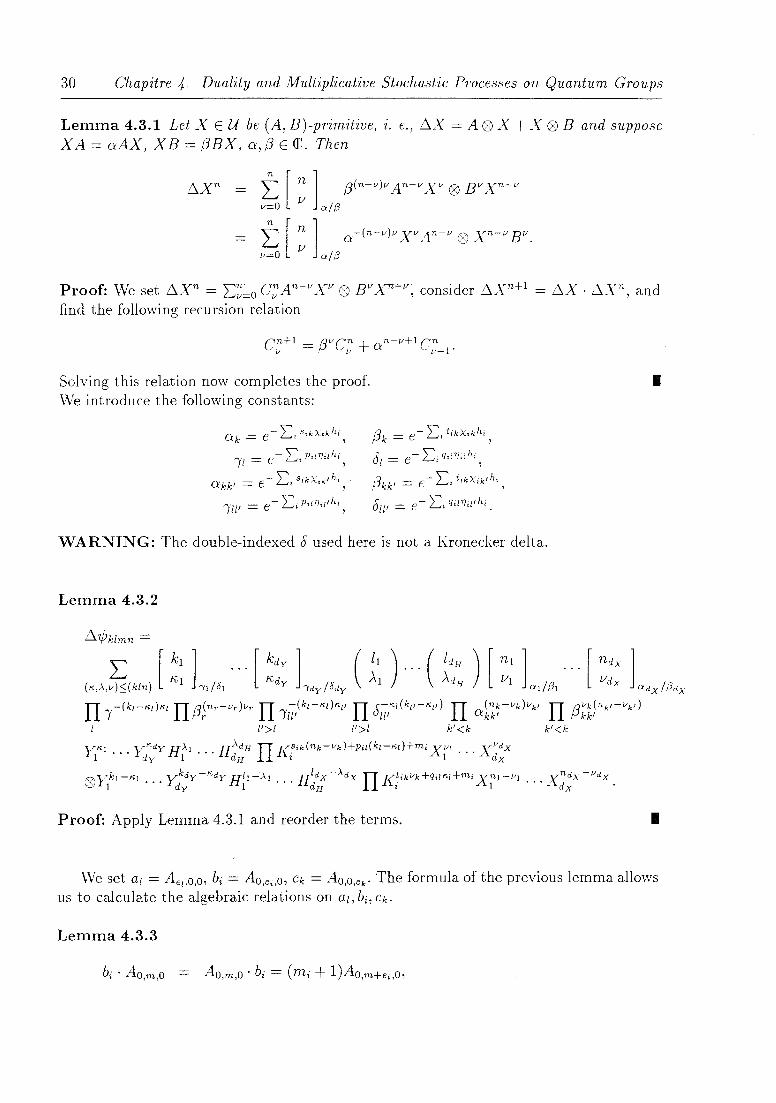
Lemma 4.3.1 Let XE U be (A, B)-primitive, i. e., ~X = A 0 X + X 0 B and suppose XA = aAX, XB = j3BX, a,j3 E <C. Then
~Xn = t [ ~ 1 j3(n-v)v An-v Xv 0 BV xn-v v=o 0i/(3
t [ ~ 1 a-(n-v)v Xv An-v 0 xn-v BV. v=o Oi/ (3
Proof: We set ~Xn = 2:~;';'0 ~An-v.xv 0 Bvr~v, consider ~xn+1 = ~X· ~xn, and find the following recursion relation
Solving this relation now completes the proof. We introduce the following constants:
ak = e- 2:. SikXikhi, - )"" v·'''·lh ÎI = e L.Ji • ,. '" "
- '\' S·kX· ,h akk' = e i...Ji· .k.', - '\' P·I"· ,h· Îll' = e i...Ji • ".1 "
j3k = e- 2:i tikXik h, ,
61 = e- 2:i QiP7il hi,
j3kk' = e- 2:i tikXik'hi ,
611' = e- 2:i qilTiil,hj .
WARNING: The double-indexed 6 used here is not a Kronecker delta.
Lemma 4.3.2
~'ljJklmn =
•
("À,~(kln) [ =: L" .. , [ ::: Ly/"Y ( i: ) ,.. ( i:: ) [ :: Lp, ,.. [ :;; L/p,x
Proof: Apply Lemma 4.3.1 and reorder the terms. • We set al = AehO,o, bi = AO,e;,o, Ck = AO,O,ek' The formula of the previous lemma allows
us to calculate the algebraic relations on al, bi, Ck.
Lemma 4.3.3
bi • Ao,m,o - Ao,m,o' bi = (mi + l)Ao,m+ei,O,

4.3. q-Exponentials :31
where (Jl) and (~) are the q-numbers introduced in the previous section. 01 nl+l (3k rk+l
Proof: Follows from the definition of the multiplication in U* in Equation (4.1) and Lemma 4.3.2. II1II These relations show that Ao is in fact a subalgebra of U* .
....-- . , .. .. 3 4 Tr 1 (" 1 l ':) .l.l.c '.J. ProposltlOll 4.'. lJ Î!k/ Ok ana D'kl Pk are no~ TûO~S Ûj um&y, then the algebra Au IS
generated by al, ... , ad y , bl , ... , bdH , Cl, ... ,Cdx with the relations
al' Ck = Ck . al, bi . bj = bj . bi,
!ill , al . al' = ,Il' al' . al, Pk' k Ck . Ck' = D'k' k Ck' . Ck,
[bi ) ad = (pil - qil)al, [bi, ckl = (Sik - tik)Ck.
Proof: Follows directly from Lemma 4.3.3. 1
If sorne ofthe ,kl !ik, D'ki/Bk are roots of unit y, then the algebra generated by al, ... ,(ldy, bl , ... , bdH , Cl, ... , Cdx is a subalgebra of Ao, which we shaH denote by Âo. For this case we introduce the algebra Û = U II, where l = {u EU; Va E Âo: < u, a >= O}.
For the following calculations we will assume that
Sik = O.
This can always be achieved by an appropriate choice of the generators, e. g., set YI rr R'i-qil YI , Xk = rr Ki- Sik X k. Then D'k = 1, D'kk' = 1, !il = 1, !ill' = 1.
We find in this case
al' Anmr if n[, = 0 for l' < l,
if r k' = 0 for kt > k.
If we assume also that 1/,i and Pi are not roots of unit y, then we have
32 Chapitre 4- Duality and Multiplicative Stochastic Processes on Quantum Groups
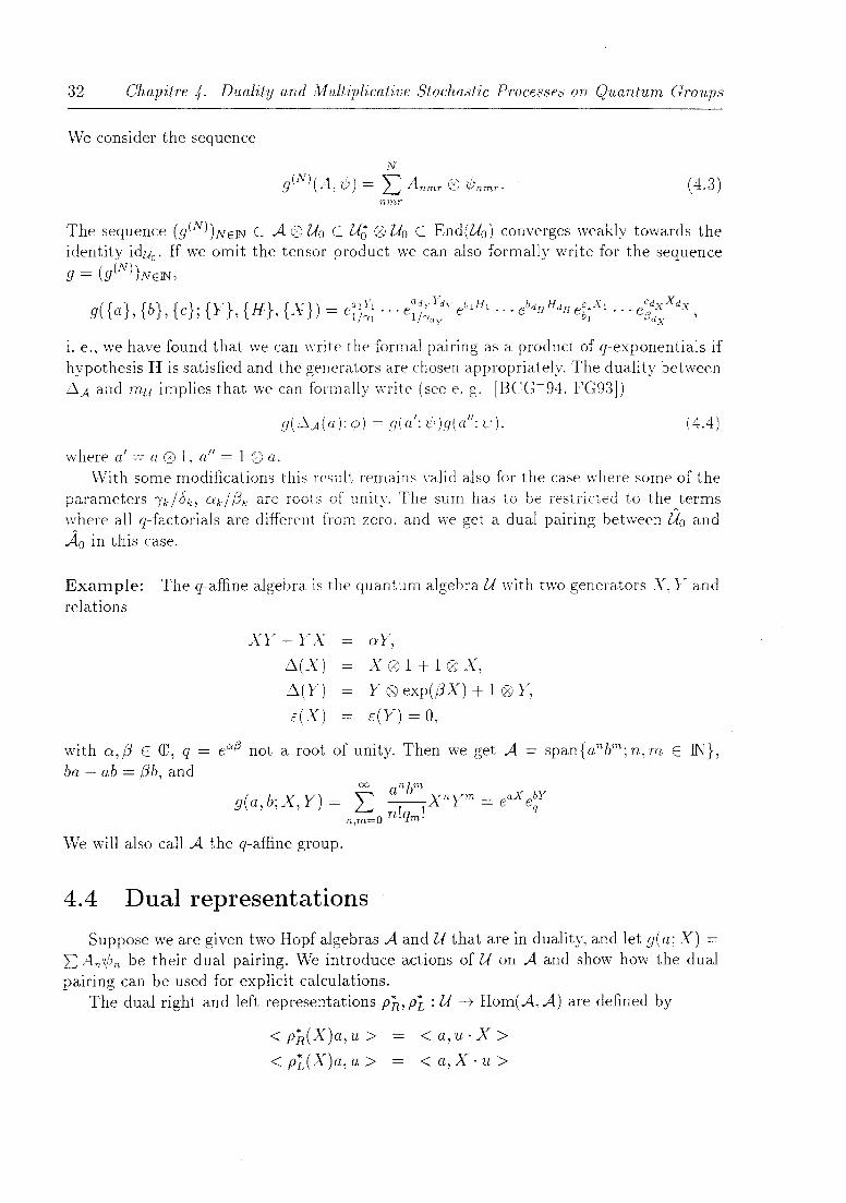
We consider the sequence
N
gIN) (A, 7/J) = L Anmr ® 7/Jnmr. ( 4.3) nmr
The sequence (g(N»)NElN C A ® Uo c U~ ® Uo C End(Uo) converges weakly towards the identity iduo . If we omit the tensor product we can also formally write for the sequence g = (g(N»)NElN,
g({a} {b} te}· {Y} {H} {X}) = ealYI •.. eadyYdy ehH1 •.• ebdHHdHeC1Xl .• • ·eCdxXdx , , , " 1 l'YI Il'Ydy b l f3dx'
i. e., we have found that we can write the formaI pairing as a product of q-exponentials if hypothesis H is satisfied and the generators are chosen appropriately. The duality between ~.A and mu implies that we can formally write (see e. g. [BCG+94, FG93])
( 4.4)
wherea'=a®l, ail = 1 ®a. With sorne modifications this result remains valid also for the case where sorne of the
parameters -fk /6k, ak/ f3k are roots of unity. The sum has to be restricted to the terms where aIl q-factorials are different from zero, and we get a dual pairing between Ûo and Âo in this case.
Example: The q-affine algebra is the quantum algebra U with two generators X, Y and relations
XY-YX
~(X)
~(Y)
é(X)
aY,
X ® 1 + 1 ®X,
y ® exp(I3X) + 1 ® Y,
é(Y) = 0,
with a,13 E <C, q = e<Y.f3 not a root of unity. Then we get A = span {anbm ; n, m E IN}, ba - ab = I3b, and
00 anbm g(a b· X Y) = '" __ X n y m = ë X ebY ", ~" q n,m=O n·qm·
We will also caIl A the q-affine group.
4.4 Dual representations
Suppose we are given two Hopf algebras A and U that are in duality, and let g( a; X) = L: An7/Jn be their dual pairing. We introduce actions of U on A and show how the dual pairing can be used for explicit calculations.
The dual right and left representations P'R, PL : U -+ Hom(A, A) are defined by
< p'R(X)a,u > < PL(X)a,u >
< a,u·X > < a,X·u >

4.4. Dual representations
for aH a E A, u EU. This leads to the formulae
P'R(X)
p'JJX)
(id 0 X) 0 LlA
(X 0 id) 0 LlA
:33
where the coproduct LlA for A is defined such that A and U are dually paired bialgebras and the X appearing on the right-hand-side is interpreted as a functional on A. We will compute the action of PHL(Xi ) on the basis {An} with the formaI pairing, and use it later , to calculate the coproduct ou. A"
Then PH is an algebra homomorphism and PL is an algebra anti-homomorphism. i. c ..
for all X, YEU.
P'R(XY)
pî(XY) PR(X)PR(Y)
PIJV)pî(X)
The key property of the formaI pairing is that multiplying the 7i'n in each term from the right (left) by Xi leads to the same result as applying the right (left) dual representation n* l 'CT \ f ." f ,r \ \ LO A :- ~~ ~1~ '-~-m : ~ fJR\-~i} \PL\-"-i)) L I1. n 111 C<LLll uc:li 1, 1. 'C.,
P'R( Xi )g( a; X)
pî(X;)g(a; X)
g(a; X)Xi
Xig(a; X).
To compute the dual representations. commute Xi past the factors e~JxJ in g(a; X) until it is next to e~;Xi, and then replace it by the operator 5i ,
{ f(qia.il-f(ail
5.f(a.) = (qi-1)ai " of(a;)
oa,
if qi #- 1,
if qi = 1,
since on the individual factors we have Xie~:xi = 5ie~:xi. For factors where qj is equal to 1, we can apply the relation eaJXJ Xie- aJX] = eaJ adX) Xi (where adXj (Xi) = [Xj , Xi])'
Quotient representations of the right and left dual representation can be constructed by factoring out a left or right ideal, respectiveIy. The duais of these representations then give corepresentations of A.
Let P : U -t Hom(V, V) be a representation of U, and {un} a basis of V. We define the matrix elements of P w.r.t. {vn } by
(4.5)
\Vith the relation g(5(a); '1/;) = g(a'; 'lj;)g(a"; 'lj;) one can show that formally
defines a corepresentation on W = span{wn }, where the W n are functionals on V defined by W n( Un') = On,nl • Anti-homomorphisms le ad to right corepresentations by Llw( wn) = W m o M nm .

34 Chapitre 4. Duality and Multiplicative Stochastic Processes on Quantum Groups
Example: We get for the q-affine algebra
pL(X) -pR(X)
pL(Y) PR(Y)
Since the dual of these representations is the coproduct of A (interpreted as right or left corepresentation of A on itself), we can use their matrix elements to get the coproduct of A:
~(a) a01+10a,
~(b) b 01 + exp(aa) 0 b.
We shaH use the quotient representation that arises from the relation X = r:
( 4.6)
4.5 Construction
Let (WdtElR+ = (Wl,···, Wtd)tElR+ be a stochastic process with values in IRd with independent increments, and assume that aH moments of Wt are finite. Then a functional <Î>tlh on IR[xt, ... , Xd], corresponding to an increment lVt2 - Wtl , is defined by <Î>tlh(X~1 ... X~d) = IE((Wt; -Wt~)nl ... (Wt~ _Wt~)nd). We can identify A with IR[x} , ... , XdJ as a vector space, if we fix a Poincaré-Birkhoff-Witt (PBW) basis{An; n E INd } for A and set z(An) = xn. We denote the functional on A obtained in this way also by <Î>tlh'
We suppose that z is chosen such that the functionals <Î>tl,t2 are positive. For example
for the q-affine group this is the case for z defined by z( ~~::!) = x~~~7 with an appropriate definition of positivity4. We do not know how to define z in general to guarantee the positivity of <Î>tlh' Nevertheless, the results below hold regardless of the positivity hypothesis.
The following construction will start with these functionals, and then recover their properties with respect to the coproduct of A.
We suppose that Wt has independent increments. For the functional <Î>t on IR[x} , ... ,XdJ this means that
where the coproduct of IR[Xl, . .. , xdl is defined by ~Xi = Xi 0 1 + 1 0 Xi. We want to construct a functional <Pt on A that satisfies the same relation with respect to the coproduct of A. To this end we define a sequence of functionals <p~N), and take its limit for <Pt, if it exists. Let
(N) A A (N-l ) <Ps,t (a) = <Ps,s+(t-s)/N 0··· 0 <Ps+(t-s)(N-l)/N,t ~ (a) for N > 1, a E A.
4. If we define the positive elements of A as the inverse image under z of the positive elements of 1R[Xl, X2].

4.6. Feynman-Kac formula 35
Loosely speaking, this corresponds to decomposing the desired pro cess into its increments via the co~roduct, and approximating its expected value by the expected value with respect to <P in each increment. We define
<P s t(a) = lim <p~~)(a) , N-+oo'
for a E A, (4.7)
if this limit exists.
Definition 4.5.1 Let Wt be a stochastic process on ]Rn with independent increments Ws,t = ~Vt - lVs ) and al! moments finite. Let further A be a Hopf algebra and z : A -t
]R[Xl' ... ,xn ] a vector space isomorphism. We cal!
the z-analogue of vVt on A, if this limit exists.
In our applications we will consider processes whose increments are stationary, i. e .. the functionals <Î> s,t and <P sot depend only on the difference t - s, in this case we can also write <Pt and <Pt.
In the following section we have a class of ex amples where this limit exists. and the expected value of the dual pairing, which in this context should be understood as a generating function, is found. For this it is necessary to extend the definition of the functional <Pt to infinite series thus:
00 co
<Pt(:L an) = L: <Pt(an), n=O n=O
if the left-hand-side converges absolutely.
4.6 Feynman-Kac formula
On Lie groups one can obtain Feynman-Kac type formulae with Trotter's product formula
lim (eX;fN ... eXd/N)N = e X1 +,,+Xd . N-+co
Let Wt be a stochastic process on ]Rd with independent and stationary increments and independent components, and
be the expectation value of an Increment, i. e., Li is the generator of l'Vi (t). Then, if we approximate the process g(W(t); X) on the Lie group defined by McKean's stochastic product integral [McK69] by g(n)(t),
lE(g(n)(t)) _ lE (II eW1Xi ... e WdXd ) = II lE (eW1X1 ... e WdXd )
(é1(XdL:>.t ... éd(Xd)L:>.t) n n:::;::' et(Ll(Xd+ .. +Ld(Xd)).

36 Chapitre 4. Duality and Multiplicative Stochastic Processes on Quantum Groups
If we take the limit on both sides we get
IE(g(W(t);X)) = et(Ll(Xd+··+Ld(Xd)).
Note that this formula still contains Trotter's product formula for the special case of a deterministic process, i. e., if Li(Xd = Xi for i = l, ... , d.
Theorem 4.6.1 (Feynman-Kac formula) Let A and U be a quantum group and a quantum algebra that are in duality, with generators al, . .. ,ad and Xl,' .. , X d, respectively, and dual pairing
qi E œ. Let p be a representation of U by operators that are bounded with respect to some norm
11·11. We set
Pi = { :ax{p; p(X;)P =1 O} if p(X;) is nilpotent, i.e. p(Xiy+1 = 0 for some integer l', otherwise.
Let z: A -+ lR[XI, ... ,XnJ be defined by z(a n ) = xl!
Suppose further that we are given a d-dimensional stochastic pmcess 1:F (t) with independent and stationary increments and independent components, and moment generating functions
co [(i)ük L i ( ü) = L _k-t- ana/y tic,
k=l k:
and moments mk(Wi(t)) = U:J k etL,(u)lu=oJ such that the series
and t m,~(lIVi(t) );(Xi )k
k=O (q,h.
are well-defined and converge (in particular, (qih =1 0, for 1 :s; k :s; Pi)' Then we have for the z-analogue of A( t) on the associated quantum gmup A
Remark: If U has a sumciently rich class of representations that satisfy the conditions of the theorem, then this relation allows us to read off aH moments of the Brownian motion. Proof: According to Definition 4.5.1 we have to consider
where 8.>t/N is the functional corresponding to an increment of Wt for !:lt = tiN. By the identification procedure outlined in the previous section this gives 8.>t/N( an) = fIi mni (1:Vi ( tiN)). If we take into account that (cf. Equation (4.4))
g(!:la; X) = g( a'; X)g( a"; X),

4.6. Feynman-Kac formula 37
where a' = a @ 1, ail = 1 @ a, then we get
<I>~N) (g( a; p(X))) = <Î>~~(g( aU); X) ... g( a(N); X))
where a(k) = 10k- 1 @ a @ I N -k, and thus
<I>}N) (g(a; p(X)))
Note that for k 2: 1 each mk(Tyi( T)) can be written as
therefore
where Ri(tjN) is sorne bounded operator. Taking the product we get
d ( Pi m (H!i(tjN)) (X)k) t d _ . t 2
II 1 + L k .. ! P '. = 1 + V L Li(p(Xi )) + V2 R(tjN), i=l k=l (qth· 1 i=l 1
where R(tjN) is also bounded. Using n;%,l av - n;;=l bv = ~~~l al ... av-l (av - bv)bv+1 ... bN , we have
for N -t 00. This conclu des the pro of, since n;;=l (1 + -h ~f=l Li(p(Xi ))) converges to
exp (t ~f=l Li(p(Xi ))). 1
VVe can now obtain a Trotter-type product formula for q-exponentials.
Proposition 4.6.2 (Trotter's product formula) Let Xi, i = 1, ... , d be bounded operators and assume that for eachi = 1, ... ,d one of the following two conditions is satisfied:
1. qi E {1} U {z E Œ; Izl =f. 1},
2. the operator Xi is nilpotent of some order Pi J i. e., XYi+l = 0, and qi E {1} U {z E Œ; ZV =f. 1 for v = 1, ... ,pd.
38 Chapitre 4- Duality and Alultiplicative Stochastic Processes on Quantum Groups
Then we have
(norm convergence)
Remark: For the second case, the q-exponential can be defined bv the finite sum eX, = , .J qi
p, :2l. f . ,rv _ . Lv=ü q,,! smce qv· # 0 for v :::; P, and )\i - 0 for v > P"
Proof: Take a deterministic process_with L.(X,) = Xi, i = L_ .. , cl,.and apply Theo-rem 4.6.1. Il
The following proposition can also be presented as a consequence of Theorem 4.6.1.
Proposition 4.6.3 The functiOlwls dcfined as the l-ana!oglle of a stochastic process luith inclependent and stationary incrulif lits and indtptndulf components forrrl a convolution semz-group.
4.7 A ppell systerns
Appell systems {hn(x); nE I\} on IR are usually characterized by the tvvo conditions
- hn (x) is a polynomial of degree n,
Interesting ex amples are furnished by the shifted moment sequences
where p is a probability measure on IR with aIl moments finite. This includes the Hermite moment polynomials
t> 0,
for the Gaussian case. These polynomials are the solutions of the heat equation
with f( x, t ---t 0) = xn. We will define Appell "polynomials" (or better Appell functions) on quantum groups in this section. It turns out that in general they are only polynomials for t = O. They provide polynomial solutions of evolution equations ofthe form ad = Lf, where L is an operator consisting of differential and difference operators.
On Lie groups P. Feinsilver and R. Schott [FS92] have defined Appell systems as shifted moment sequences. They are introduced as the expectation of coordinate functions shifted by right or left multiplication of the argument by a group-valued random variable. Let

4.7. Appel! systems
J : G ----t Πbe a function on a Lie group G, g(a) an element of G, and g(Z) a G-valued random variable, then we can evaluate
IE(J(g(a)g(Z))) and IE(J(g(Z)g(a)))
vVe choose for J a set of basis elements {Am; m E ]Nd} of the algebra of functions on G, then the right and left Appell systems (w. r. t. Z) are defined as
IE(An(g(a)g(Z))), IE(An(g(ZJg(a))).
The Appell functions are again functions on G. We rewrite these equations in terms of the coproduct (note J(glg2) = 6.J(gl,g2)).
Definition 4.7.1 The Appel! systems on A with respect ta the basis {Am} and the randam variable Z are defined as
Remark: Note that for quantum groups Z exists only as a functional on A. If we use the parametrization introduced by the formaI pairing then we can express the Appell systems in terms of the basis {An} and the matrix elements (cf. Equation (4.5)) with respect to this basis:
h~(a) = (id Q9 Z) (~l'yf~m(a) ® Am) = ~ Af~m(a)Z(Am)
(id® Z) (LAm Q9 i11~n(a)) = LAmZ (Af~m(a)) m m
h~(a) I: Z (lv1~m(a)) Am = L Z(Am)Af~m(a). m m
The Appell systems have the following transformation property
r
r
Interesting relations to evolution equations arise if we consider the Appell systems with respect to multiplicative stochastic processes. Suppose now that Zt has generator L, 1. e.
Then
(Zt ® id)(g( a; X)) = exp tL.
Oth~(a;t)
Oth~( a; t)
PR(L)h~(a; t)
PL(L)h~(a; t)
40 Chapitre 4- Duality and Multiplicative Stochastic Processes on Quantum Groups
i. e., h~, h~ provide solutions to evolution equations (where h~(a; t = 0) = h~(a; t. = 0) = An).
Let Ri, Li be the raising and lowering operators wi th respect to the basis {An}, wi th
for some coefficients Cni, then
R- tLR -tL i = e i e ,
are raising and lowering operators for the Appell system. We also define analogues of relative Appell systems, i. e., Appell systems on homoge
neous spaces. Let (V, ~v : V -t A ® V) (or (V, ~v : V -t V ® A)) be a left (or right) corepresentation, then the Appell system on V with respect to a basis {vn } of V and a functional Z on A are defined by
(Z ® idv ) 0 ~Vvn,
(idv ® Z) 0 ~Vvn).
Examples: We start with a very simple example. Consider the process on the q-affine group (with a = -1) obtained from the one-dimensional Brownian motion (0, Bd on IR2•
Then 1> ( ap(X) bp(Y») _ tp(y)2
t e eq - exp 1 + q
for aIl representations where p(Y) satisfies the conditions of Theorem 4.6.1. Take e. g. V(N) = span{bn;n = O, ... ,N} and p(X) = bab, p(Y) = 6b (cf. Equation (4.6)). The moments of this process are
n odd n even, n = 2m
and the right Appell polynomials are
These polynomials are solutions of
62 aff(a,b;t) = _b f(a,bi t )
l+q
In the limit q -t 1 they tend to Hermite polynomials. We can also try to associate a density to this process by requiring 1>t(p(b)) = fp(x)f.1(dx) for all polynomials p(b). For o < q < 1 such a density exists and can be characterized with the help of the random variable Y = (l-q) L~o Xi, where the Xi are independent, and exponentially distributed with respective means qi. The characteristic function of Y is lE(eitY ) = e~t, see [Fei87].
{8. Extension of the construction 41
Thus <Pt IEy ( è YU ) = <P t ( e~U) = exp :~2q' i. e., bY is Gauss-distributed with mean zero and
variance (J"2 = l~q' By [Fei87, Theorem 3] this characterizes the distribution uniquely.
Now look at Xt = (0, Nt), where Nt is a Poisson process, IE(euNt ) = exp(t.\(eU - 1)). By the Feynman-Kac formula we have
We take again p(Y) ~ Ob, then (e;(Y) - 1 lb" ~ I:~"l [ ~ l, b"-k, this yields the associated
Appell polynomials hn(b; t) = exp(t.\(e~(Y) - l))bn. We look now at the stochastic process obtained from the two-dimensional Brownian
motion (At, Bt) on IR2. We calculate the Appell system corresponding to this process and the corepresentation that is obtained as the dual of the representation pr on the polynomials in one variable, Pr(X) = x3x + r, Pr(Y) = ù5x (cf. Equation 4.6). We choose the functions C~;q(x) given by
where (r)m = r(r + 1)'" (r + m -1). For q = 1 these are Gegenbauer polynomials. They satisfy
LC~;q(x) = (n ~ ,)2 C~;q(x)
with L = t(x3x + ,)2 - 12q' For the Appell system one obtains
hr () (( n + ,)2 ) c,r ( ) n X; t = exp 2 t n;q x .
They are solutions of 3tu = Lu. The C~;q(x), n E IN form a basis for IR[x], if q is not a root of unit y, and r =1 -k for k E IN, and the Appell polynomials corresponding to other choices of the basis can be computed from those defined above.
4.8 Extension of the construction
From a probabilistic point of view the preceding construction is far from satisfactory. We can only evaluate the process at one fixed time. But the interesting feature of a stochastic process is exactly that it is a parametrized family of random variables, i. e., that it is defined for an values of the parameter. In this section we will construct a larger algebra that can be understood as the tensor product of A over t E IR+. On this algebra we can define a functional that corresponds to the distribution of the process (see also [ASW88, Sch93]).
Let Tn = {t = (h, ... ,in);ti E IR+,t1 < i2 < ... < in} C IR~, Ta = {ID}, T = U~=aTn, i. e., Tn contains aIl subsets of ~ with n elements, and T aH finite subsets of IR+. The

42 Chapitre 4- Duality and Multiplicative Stochastic Processes on Quantum Groups
set T is partially ordered by inclusion. For each t = (t l , . .. , tn) E T we set At = Ac~*1 as a vector space, where Itl = n is the length of t. Let 'l/Jt : At -7 A01tl be defined by
'l/Jt(al 0··· 0 alti) = (al 0 1 0··· 0 1)(~a2 0 1 0··· 0 1)··· (~Itl-Ialtl) (4.8)
where the multiplication on the right hand side is the usual multiplication mOiti in the tensor product algebra A01tl.
Lemma 4.8.1 These maps are vector space isomorphisms.
Proof: Let '112 : A 0 Â--+ A 0.A_be defi.ned by .W2(a 0 b} = (a 0 l)(Llh), . .i. e.,W2 (m 0 idA) 0 (idA 0 ~). '112 is an isomorphism, and its inverse is given by <I>2 = (m 0 idA) 0
(idA 0 S 0 idA) 0 (idA 0 ~). Here is a diagrammatic proof of the relation '11 2 0 <I>2 = idA0A , and <I>2 0 '11 2 = idA0A can be shown similarly.
=
For the interpretation of this diagram see [Maj93a, Maj95b]. Not using the diagram technique we can write the proof as 'l12 0 <I>2 = (m 0 idA) 0 (idA 0 S 0 idA) 0 (idA 0~) 0
(m 0 idA) 0 (idA 0~) = (m 0 idA) 0 (idA 0 m 0 idA) 0 (idA 0 idA 0 S 0 idA) 0 (idA 0 ~ 0 idA) 0 (idA 0 ~) = (m 0 idA) 0 (idA 0 e 0 idA) 0 (idA 0 E 0 idA) 0 (idA 0 ~) = idA0A
Note now that 'l/Jt can be written as
This completes the proof.
This lemma allows us to equip At with an algebra structure by the definition
mt(a, b) = 'I/J;I(m0 Itl('l/Jt(a), 'l/Jt(b))).
• ( 4.10)
Define it',t : At' -7 At for t' E t by inserting the unit element 1 in the factors corresponding to the indices of t that are missing in t', e. g. for t = (t l , ... , tn) and t' = (t b ... , tj-h tj+!,"" tn) we have i t',t(aI0" '0an-d = aI0··· aj-1010aj+! 0··· an-l' Note it',t 0 itll,t' = itll,t and that these mappings are injective. Related to these are the maps jt',t = V;t 0 it',t 0 'I/J;;l : A01t'I -+ A01tl. One verifies that for these maps also jt',t 0 jt",t' = jt",t, and that for t = (t l , ... , tn) and t' = (t l , ... , tj-h tj+l, ... , tn) we have jt',t(al 0 .,. 0 an-d = al 0 ... aj-l 0 ~aj 0 aj+! 0 ... an-l, i. e., jt',t decom-poses the increment from tj-l to tj+! into the increments from tj-l to tj and from tj to tj+! via the coproduct, whereas for t = (ft, ... , tn) and t' = (t l , ... , tn-d we have jt',t( al 0 ... 0 an-l) = al 0· .. an-l 0 1, i. e., for increments corresponding to times larger than the maximal time represented in t' the unit element 1 is adjoined.
Proposition 4.8.2 The algebras (At, mt) and the mappings it,t' form an inductive system and thus define an algebra À with injective algebra homomorphisms it : At -7 À such that .. . Zt 0 Zt',t = Zt"

4.8. Extension of the construction
Proof: To prove the proposition we have to show mt 0 (it',t @ it',t) = it'ot 0 mtl, i. e., that the maps it',t are algebra homomorphisms with respect to the multiplications mt, mtl. It is clear that Ù,i is an algebra homomorphism, since the coproduct .0.. is one, and adjoining the unit element is one, too. Now
'ljJ;1 0 mOiti 0 (1jJt @ 'lj!t) 0 ((1/);1 0 jt',t 0 'ljJtl) 0 ('ljJ;1 0 jtl,t 1/ltl))
'ljJt- l 0 mOiti 0 (jtl,t 0 jtl,t) 0 ('ljJt' @ 'ljJtl) = 'ljJt- 1 0 jt',t 0 m0lt'l 0 ('ljJt ' 'I/'tl)
Zt',t 0 mtl.
Il
This algebra plays the rôle of the canonical representation of the process. If A is generated by al, ... , an, then À. is spanned by the polynomials in {(al, i), ... , (an, i); t E lR+} (we also write at for a pair (a,t), a E A. t E lR+). For the Hopf algebras A the algebraic relations are sufficient to order the factors such that the index corresponding to time increases from the left to the right, i. e., À. is spanned by the monomials
where i = (il,"', tm) varies in T. The functional on À. can now be defined with the help of the maps . Let (<I>dtElR+
be the family of functionals defined in Section 4.5. Then we define
for a E At, t E T.
Proposition 4.8.3 The functionals {<Î>t; t E T} determine a unique functional <Î> on À. such that <Î> 0 it = <Î>t.
Proof: VVe have to show that <Î>t' = <Î>t 0 itl,t for aH t' ç t. The functionals <l>t in Section 4.5 form a convolution semi-group, i. e., (<I>t 0 <l>s) 0.0.. = <l>t+s, and, more generally, for i = (il, .. . ,tn ) and t' = (i vp '" ,tvk ) ç t,
The proposition now follows from the definition of <Î>t = (<I>tl @ ... @ <l>tn-tn_l) 0 1;t and of Zt',t. Il
vVe define a family of maps (cpt )tElR+, CPt : A --t À. by
(4.13)
vVe have not considered * -structures here, but one immediately sees that (cpt )tElR+ is a quantum stochastic process with respect to aH other requirements, i. e., it is an algebra homomorphism from algebra A to the algebra À. with the unital functional <Î>. The onedimensional distributions of this process are exactly the functionals <l>t = <Î> 0 CPt.

44 Chapitre 4- Duality and Multiplicative Stochastic Processes on Quantum Groups
The following theorem summarizes the main results of this section.
Theorem 4.8.4 {'Pt : A -+ (À, cf,); t E IR+} is a quantum process with independent and stationary incrementsJ i. e' J it satisfies
1. 'Pt : A -+ À is a unital algebra homomorphism for ail t E IR+,
2. the functionals <Pt = cf, 0 'Pt form a convolution semi-group, i. e.,
for ail a E A J t,s E IR+.
Example: For the q-affine group À is spanned by
{ nI bml nPbmp • . J:\T t t tIR· INP} atl tl ···atp t p ,p E ll~, 1< 2 < ... < P E +,n,m E 1
The commutation relations bet\'\'een elements corresponding to the same time t remain unchanged, those between elements corresponding to different times s < tare determined by
as·ah as . bt + {Jbs,
bs • at - .Jbs ' q-1bs . bt + (1 - q-l )b;.
4.9 Conclusion
We have shown how to construct stochastic multiplicative processes on quantum groups. For the analogue of processes with independent and stationary increments we proved a Feynman-Kac type formula. Appell systems have been defined and shown to be solutions of evolution equations.
The positivity of the constructed process is not a priori clear, but depends on the choice of the identification of A and IR[XI, . .. ,d]. Nevertheless, the proof of the FeynrhanKac formula doesn't require positivity, while the other results presented do not depend on it. Finding good criteria for which cases the obtained process will be positive is an open problem, for sorne results about positive functionals on quantum groups see [Koo91].

Chapitre 5
Diffusions on Braided Spaces
Uwe Franz René Schott 5
Résumé
The notion of q-Brownian motion introduced by Majid is extended to braided spaces corresponding to a generic R-matrix, and combined with the theory of quantum probability. This leads to a definition of diffusions on these Spaces. The corresponding heat equations (difference-differential equations) are solved in tenns of Appel! polynomials (i.e. shifted moment systems). Sorne examples of interest for applications are given.
5. CRIN-CNRS, BP 239, Université H. Poincaré-Nancy 1, F-54506 Vandœuvre-lès-Nancy, France, Email: [email protected]
45

46 Chapitre 5. Diffusions on Braided Spaces

5.1. Introduction 47
5.1 Introduction
The applications of diffusions in physics go far beyond the description of the physical phenomenon they are named after. Functional integrals can be used to solve partial differential equations, cf. the celebrated Feynman-Kac formula. Wiener integrals are very close to Feynman path integrals. Another interesting application of diffusions is the stochastic mechanics of Nelson [NeI66].
vVe will present an approach to diffusions on braided spaces here. Diffusions on manifolds are characterized by two properties, the first being their Markov property, i.e. that at every instant t they start again, and their evolution does not depend on their history, but only on their distribution at time t. This gives rise to a semi-group and this property will also play a central role for the study of diffusions on braided spaces. The other propert y, i.e. that they have continuous sam pIe paths. does not have a direct counterpart on braided spaces. We replace it by the condition that diffusions can be obtained as the limit of a (simple) random walk.
The motivations for our approach come from two directions. First, there is MajicI's random walk approach to Brownian motion on the braided line and on anyspaces r1\1~J'rl':>rl 1\.fDDrlA] 'U" "vt=ncll,;L' rl=-hn;t;,w, tn (nCPl1rl" \ rliffllci"nc nn rn1ulti ,lirnpn"inn,,] t ... V1d Û·)U~ lV.l.lt·..l ·7'-1 • lil'\..:. L.''\.LJLll .1.1,1 ..... 1 \.-t.vl.l.liJ.L'.1V,LL V"-" \!-,u ............ 4-'-"'-'-,,- J ............ .l-.-""'-'-' .... "' .... -'-'--' """"."--.L ->..>--"- ........ - ... --...... ... .L ........ ~- .... _'- ______ ,_
braicled spaces and, using coalgebraic limit theorems due to Schürmann [Sch93], give their explici t form. This allows to consider semigroups of functionals and IVlarkovian transition operators, as weIl as the associated heat equations, and to introduce Appell systems as their polynomial solutions. Heat kernels, i.e. the densities of the functionals are also considered.
The second ingredient, l'vI. Schürmann's theory of quantum Lévy pr~)Cesses, cornes into play to assure the existence of the associated processes, e.g. as operators on a Hilbert space. vVe propose a definition of * -structures for braided Hopf algebras (differing from those due to S. Majid), and give several examples that satisfy our axioms. Then we generalize M. Schürmann's definitions and a result assuring the positivity of the convolution of positive functionals under certain conditions to braided groups.
To distinguish the two levels of the constructions, we call the functionals and semigroups obtained via S. Majid's construction pseudo-diffusions, and reserve the name diffusion for the case where the processes can be realised as operators and are Lévy pro cesses (i.e. independent increment processes) in the sense of M. Schürmann.
This paper starts with a brief summary of the definition of braided spaces and their main properties in Section 5.2. vVe also introduce sorne basic notions of quantum pro bability such as independence and Lévy processes, including a few generalizations that are necessary to apply the existing theory to braided spaces.
The next section (Section 5.3) shows how (pseudo-) diffusion processes can be constructed on generic braided spaces associated to a pair of matrices (R, RI). The approach is based on the idea that diffusions can be approximated by random walks on lattices. This replaces the classical condition of the continuity of sample paths. We obtain the explicit form of the limiting pro cess as the chosen time interval and the lattice parameters tend to zero.
Section 05.4 investigates the relation between the diffusion processes and associated evolution equations. These equations are of the form (Ot - L)u = 0, where L is an ope-

48 Chapitre 5. Diffusions on Braided 5paces
rator consisting of linear and quadratic terms in the braided-partials fJi. A ppell systems (introduced as shifted moment polynomials) are shown to be solutions of the evolution equation. We investigate their properties.
In Section 5.5 we discuss briefly how density functions can be introduced. We close with a few final remarks in Section 5.6.
5.2 Preliminaries
5.2.1 Braided spaces
Let us recall the notion of a braided group. This is (B, m,l, ~, E, 5, 'li) where (B, m, 1) is a unital associative algebra, (B, ~, E) a coalgebra, 'li a brai ding (satisfies the braid relations), and 5 an antipode (i.e. m 0 (id ® 5) 0 ~ = m 0 (5 ® id) 0 ~ = 1 0 E). The difference that distinguishes braided groups from quantum groups (Hopf algebras) is that now ~ is braided-multiplicative, i.e.
where m~ is defined by m~((a®c)(b®d)) = a'll(c®b)d. For a more detailed and elegant introduction see e.g. [Maj93a, Maj96].
Braided spaces are braided groups with a particular form of the product and coproduct, see below. They are a generalisation of superspaces, there are braided lines, braided planes, braided matrices, etc., aIl in analogy with superlines, superplanes, etc. Braided spaces are the elementary building blocks of the 'braided world' or braided linear algebra.
For a pair of invertible matrices (R, Rf) that satisfy
(i) Rl2Rl3R23 = R23Rl3Rl2 (i.e. the Quantum-Yang-Baxter equation),
(iii) (PR + l)(PRf -1) = 0,
where P is the permutation matrix (X2 ® xlP = Xl ® X2), and Rl2 = R ® id, R23 = id®R, etc., there exist two braided Hopf algebras V(R, Rf) and VV(R, Rf) with generators VI, ... ,Vn and Xl, .•• ,Xn and relations
- for V(R, Rf):
~Vi
'lI(v i ®vi )
vivi
Vi ® 1 + 1 ® vi,
RikilVI 0 v k ,
Rfi ki /v1v k ,
0,

5.2. Preliminaries 49
- for VV( R, R'):
Xi ® 1 + 1 ® Xi,
Rk l Xl®Xk ij,
XiXj R,k l XZXk i j,
-Xi,
0,
see [Maj93b, Theorem 1]. Here the first two indices (i, k) correspond to the first factor in the tensor product, and the last two (j, l) to the second factor. \Ve use the summation convention, i.e. indices that appear twice (once as subscript and once as superscript) are summed over. In a shorter notation this becomes
for V(R, R'): D..v = v ® 1 + 1 ® v, W(VI V2) = R12V2 VI, R~2V2VI S(v) = -v, é(V) = 0,
- for VV(R, R'): D..x = x ® 1 + 1 ® X, W(XI ® X2) = X2 xIRI2' X2XIR~2 = XIX2,
S(x) = -x, é(X) = O.
The braided Hopf algebras V(R, R') and 1F(R, R') are called the braided vectoT space and the braided covectoT space associated to (R, R'). For a detailed development of their properties see also [Maj93c, Maj93a, Maj96]. We will summarize here only sorne facts that are used in this presentation.
Let S {l, ... , n} be the set of aU finite sequences composed of the elements l, ... , n, i.e. S {I, ... , n} = {0; l, ... ,n; Il, 12, ... ,1212; lll, ... }. Set va = v ak .•• val if a = (al' .. ak) E S {l, ... , n} \ {0}, and v iJJ = l, and analogously, but in reversed order, for X a = X al .•. X ak .
Then {va;a E S{l, ... ,12}}, {xa;a E S{l,oo.,n}} span V(R, R') and V'(R, R'), respectively. Notice that in general these sets do not form a basis. But a basis can easily be extracted from them, if one orders them, and eliminates all elements that are linearly dependent on those that precede them.
The algebras V(R, R') and V'(R, R') are IN-graded with
V(R, R,)(r)
V'(R, R')(r)
span {va; a E sr {l, ... , 12 } }
span {xa ; a E sr {l, ... , n}},
where sr {I"", 12} ç S{l, ... , 12} contains only the sequences of length r. This allows us to define a scaling s(À) : V'(R, R') --t V'(R, R') by s(>.)a = >.deg(aJ a for homogeneous elements a E V'(R, R') or V(R, R').
V(R, R') and l/'(R, RI) are mutually dual with the definition
where laI, Ibl is the length of a, b E S{l, ... ,12} and
[mi R] [mi Rl!
1 + (PRh2 + (PRh2(PRh3 + ... + (PR)12'" (PR)m-l.m,
[2; Rlm-l.m[3; R]m-2.m-l.m ... [mi Rh, ... ,m
(5.1 )
( 5.2)
50 Chapitre 5. Diffusions on Braided Spaces
(cf. [Maj96, Section 5]). This defines also an action of V(R,R') on V"(R,R') (and vice versa) by
p(vi) fi = « vi,. > ®id) 0 .6.,
p(Xi) ai = « ',Xi > ®id) 0 .6..
Braided exponentials exp( xlv) are defined as solutions of
ai exp(xfv) = exp(xfv)V i ,
exp(xlv)âi = Xi exp(xlv),
(c ® id) exp(xlv) = 1
(id ® c) exp(xlv) = 1.
If the braided integers lm; Rl are aIl invertible, the exp(xlv) is given by
vVe will assume that this is the case in what follows. or rather that there exists a braidedexponential exp(xlv) = L xaF(m; R)'bvo, see [Maj96, Section .5.4].
5.2.2 Quantum probability and quantum Lévy pro cesses
A quantum probability space is defined as a pair (A, <I» consisting of a * -algebra A and a state (i.e. a normed positive linear functional) <I> on A. and a quantum random variable j over a quantum probability space (A, <I» on a *-algebra B is a *-algebra homomorphism j : B --+ A. In particular, every element a of A defines a random variable on the free algebra Œ < z, z* > with two generators z, z* (with the obvious *-strudure), simply set j(z) = a, j(z*) = a*, and extend as a *-algebra homomorphism. If a is self-adjoint, then we can take B = Œ[z], with the *-structure defined by z* = z, i.e. the algebra of complex-valued polynomials on the realline.
A central notion to this work is that of independence. Independence in quantum probability is closely related to the notion of products of (*- )algebras, as e.g. the tensor product or the free product. The kind of independence we use here is related to tensor product of algebras in braided categories, it generalizes the tensorial independence introduced by M. Schürmann for braidings that arise from an action 0: and a coaction , of sorne group algebraŒIL as 'li = (o:®id)o(id®T)O(!®id) or 'li = (id®o:)o(T®id)o(id®,). For a more general definition of independence see [ALV94], for a general analysis of the notion of independence we refer to [Sch95a, Spe]
Definition 5.2.1 The quantum random variables j1,j2,'" jn B --+ A are called w-independent (w. r. t. the state <l») if
(i)
for al! permutations (J E S( n) and al! b1 , ••• , bn E B) and

5.2. Preliminaries 51
(ii)
for ail 1 :S; k < 1 :S; n.
Remark: If A is commutative, then (i) is equivalent to the condition used in classical probability theory:
(i')
for aH bl , ... , bn E B.
'vVe will call j1, ... , jn pseudo-( W- )independent, if they satisfy only (i ') and (ii). For many of the algebraic aspects this behaves like 'true' independence.
Let us investigate, wh en two quantum random variables on a braided space V- are (pseudo-) independent. Condition (ii) implies that jl (x;) and j2 (x j) satisfy the braid relations. Therefore we can assume A = ~T_®V-, and jl(U) = U 1, j2(U) = 1 ® U (take <Î> = <I> 0 (jl ® j2)' Condition (i'), i.e. pseudo-independence, is now equivalent to the fact that <Î> can be factorized into <Î> = 4/2) ® rjJ(1), w here 4>( i) = <I> 0 ji ,i = 1, 2. Thus the joint distribution of jl and j2 is uniquely determined by the marginal distributions.
Condition (i) is stronger, for independence in the sense of the preceding definition we need a kind of invariance or commutativity condition in addition to the factorisation, namely 4>(1) ® rjJ(2)(u ® v) = 4}2) ® 4>(1) (W(v ® u)), or rjJ(1) ® 4>(2) = W(rjJ(2) 4>(1)), i.e.
f.. ® 4>(2) and rjJ(l) ® f.. have to commute. We will study here time and space homogeneous Markov processes, i.e. Lévy processes.
Definition 5.2.2 A quantum Lévy process on a (braided) *-Hopf algebra B is a quantum stochastic process {jt : B -----+ (A, <I> ) 1 t E IR+}, such that
(i) {jtli E IR+} has independent increments, i.e. jSlt!' ... ,jsntn are (W-)independent for al! 0 :S; SI :S; il :S; ... :S; sn :S; in, where the increments are defined by jst =
(js 0 5) * jt = mA 0 ((js 0 5) ® jt) 0 6.,
(ii) the distTibution <I> 0 jst of an increment jst depends only on t - s (stationarity),
(iii) jst converges to jss in distTibution for t '\. s (weak continuity),
(iv) jsu = jst * jtu(= mA 0 (jst ® jtu) 0 ~B) for all O:S; s :S; t:S; u.
vVe shaH speak of pseudo-Lévy processes, if the increments are only pseudo-independent. In this case we will not insist on the positivity of the state either, we study pseudo-Lévy pro cesses (and pseudo-diffusions, see below) only to illustrate the algebraic part of the theory.
It follows from the general theory (cf. [Sch93]) that a Lévy process is uniquely determined by its marginal distributions !.pt = <I> 0 jt, that the marginal distribution form a
52 Chapitre 5. Diffusions on Braided Spa ces
convolution semigroup, i.e. <po =~, <Ps*<Pt = (<Ps®<Pt) oL\. = <ps+t, and that there exists a unique functional L, called generator, su ch that <Pt = exp( tL). Vice versa, the semigroup, and thus the process, is also uniquely determined by its generator. All this is also true for pseudo-Lévy processes.
Let us now look at the differences. The independence of the increments implies 'li (e tL ® esL ) = esL ® etL, and thus W(L ® L) = L ® L, i.e. L ® ~ and ~ ® L commute (in the convolution algebra of functionals on V"®VT AIso, since the semigroup is positive, L is conditionally positive (i.e. positive on the kernel of ~), to see this just differentiate w.r.t. t, and hermitian. In the sequel, when we speakof Lévy processes,. we will always assume that our states 4> (on A) are 'l'-invariant in the sense that 'li (4) ® u) = u ® 4> for aH functionals u : B -t <C, i.e. that we can pull it across braidings.
If L is a hermitian, conditionally positive, and 'l'-invariant functional, then all the convolution powers of L are positive (see Lemma 5.2.4), and the semigroup associated to Lis positive. Thus there exists a Lévy process with <Pt = exp( tL) as marginal distributions.
We summarize this in the following proposition.
Proposition 5.2.3 Let A be a (braided) (*-)Hopf algebra (cf. Subsection 5.2.3).
(i) There is a one-to-one correspondence between pseudo-Lévy processes {jt It E IR+}, normed convolution semi-groups {<ptlt E IR+L <Pt = exp(tL) = ~ojt, andfunctionals
L = tt<ptlt=o with L(l) = 0 on A.
(ii) There is also a one-to-one correspondence between Lévy processes, normed positive convolution semigroups of 'li -invariant states, and 'li -invariant, hermitian, conditionally positive functionals.
5.2.3 A remark on braided *-Hopf algebras
S. Majid has studied *-structures on braided Hopf algebras in a series of articles [Maj 94, Maj95a, Maj95c]. An essential result of his work is a new set ofaxioms for the braided case. But we found it necessary to use different axioms here, in particular, it is important for our purposes that the coproduct is a * -algebra homomorphism.
We fix the *-structure in the tensor product A®A by the condition that the canonical
inclusions A ~ A®A ~ A are *-algebra homomorphism, i.e. (1 ® a)* = 1 ® a* and (a ® 1)* = a* ® 1 for all a E A. This implies (a ® b)* = 7jJ(b* ® a*) for an a, b E A. Then we say that A is a (braided) *-Hopf algebra if (A, *) is a *-algebra, and L\. and ~ are *-algebra homomorphism (with the *-structure of A®A defined as above!).
For examples of braided *-Hopf algebras satisfying these conditions see Subsection 5.3.2.
Let us outline the main steps and ideas of their construction. We start with a braidedcovector space V"(R, R') with R, R' of real type l, i.e. Ri/ l = RI kii. S. Majid has defined a map * for this case that goes from V"(R, R') to VeR, R'), and vice versa, cf. [Maj95a, Lemma 2.1]. The free product VeR, R') * V"(R, R') thus becomes a *-algebra with this map, and the coproducts of VeR, R') and V"(R, R') define a *-algebra homomorphism ~ : VeR, R') * V"(R, R') -t (V(R, R')®V(R, R')) * (V·(R, R')®V"(R, R')). Now it turns

5.3. A construction of (pseudo-) diffusions on bmided spaces 53
out that (V(R, R') * V'(R, R'))(2)(V(R, R') * VV(R, R')) can be obtained as a quotient of (V(R, R')(2)V(R, R')) * ClF(R, R')@VV(R, R')) in such a way that the canonical projection is a * -algebra homomorphism, and that V (R, R') * V' (R, R') is a braided * -Hopf algebra in the sense of our definition with 6. = Tt 0 6.0 , Set Xli = Xi (2) 1, v~ = vi @ l, ;1:2i = 1 (2) Xi, and v; = 1 @ vi, then the relations defining the braided * -Hopf algebra structure of V(R,R') * VV(R, R') are
XiXj
xi 6.( Xi)
S(x;) =
( .T ,)* a.!
;'C2i X lj ;'C2iV l]
R ,k 1 X[Xk i ),
v' ,
Xli + X2i,
-Xi, S(v i ) = -v" R,k 1
X a ,I;1'a.k , .i,
v ' cr,
Rk 1 X " i j li·' 2k,
R- k), ' 1 , ,l1 .f2k·
(V i )* Xi, ê:.(v i ) Vl'+V2"
dXi) = ~(vi) = 0
'l'a] V,,'
( " i \ '" l' Cl )
l'Z' .Tl]
U1) U2'
R,j i 'L' k,,, 1 1 1.: Cl va , Ct = 1,2,
Ct = 1,2,
where il is the second inverse of R, i.e. the solutioll of L R\jIR!.:"r;' = L Ri J?k n m j = rSinrSml . vVe observe that, with the definitions xi = Vi, .'C~,i = Va', the 'v-v' relations follow from the corresponding 'x-x' relations, and the second line of the braid relations from the first (\vhere we use that R. R' are real type I).
Note also that \If ( Xk L .Th?'l i) = L :r1iv1 i xl.:, \If ( vI.: L XliUl i) = L XliV]i vI.:.
Thus the functionals that are non-zero only on L Xivi are \If-invariant. vVe prove the following.
Lemma 5.2.4 Let A be a bmided *-bialgebm (in the sense of the preceding definition, i. e. the *-structure in the bmided product algebm A@A is given by \If 0 (* *) 0 T. and ê:. is a *-algebm homomorphism)) and let 1> a \If-invariant positive functional on A. and e a
positive functional on A. Then 1> * e = (1) (2) e) 0 ê:. is also positive.
Proof: Let a E A, and ê:.(a) = Li a}l l @ a1 2l (Sweedler's notation). Then ê:.(a*) =
Lj w ((a)2l)* (2) (a)ll)*) and therefore (4) (2) e) 0 ê:.(a*a) = (1) e) 0 (m @ m) 0 (id @
\If (3) id) 0 (w (2) id (3) id) (Li,j (a)2l)'" (2) (a)1))* (2) a~ll @ ai2») = e 0 (4) (3) m) 0 (w 0 id) 0
(id @ m id) (Li.j (a?l)* Qi) (a?l)'" @ a}l) Qi) a}2 l ) = Li,j e (( a)2l)* aFl) 1> ((ay»)'" al l ») 1S
positive, since it is the Schur product of two positive definite matrices. 1
5.3 A construction of (pseudo-) diffusions on braided spaces
Following Majid we n.rst define a quantum random walk. Consider a classical random walk on the lattice. We assume that the pro cess can only jump from a lattice site x to a finite number of other sites x + di, i = 1, ... , k. If at time t the particle is located at x,

54 Chapitre 5. Diffusions on Braided Spa ces
then it will be at x + di at time t + tlt with a probability pi, 0 :::; Pi :::; 1, and naturally the probabilities add to one,
i=l
In classical probability theory there corresponds an evolution operator to this, that maps a function (i.e. an observable) at time t to the corresponding function one time step later
k
ft(x) t-+ !t+tlt(-x) = L pdt( x + di)· i=l
Let <jJ(d i ) be the functional corresponding to evaluation of a function at di, I.e. <jJ(di )
f(x) t-+ f(d i ), then the above equation can be written as
where <jJ = LPi<jJ(d;) and tl stands for the usual cocommutativecoproduct on IR[Xl"'" x n ].
This can be done in the same manner on braided spaces and quantum groups, if one chooses an appropriate functional <jJ. The problem here (in dimension> 1) is that one can not define the <jJ(d;j sim ply as replacing the variables Xi by the components of the vectors dj = (dj1 , .•. , djn ) due to the non-commutativity. One possibility is to bring the variables into sorne fixed order (i.e. fix a basis of monomials) and replace them then by the dji . We shall see later that in the limit only the choice on the quadratic and linear terms matters.
A functionàl <jJ(d) that corresponds to evaluation at d = (dl, ... , dn ) should satisfy
FI: <jJ(d)(I) = 1, or equivalently <jJ(d)lv"(R,RI)(O) = C,
F2: evaluation on the generators gives the components of d, i.e.
for i = 1, ... , n,
F3: it has the correct behavior with respect to a rescaling of d, more precisely,
for homogeneous a E VY(R, R').
But these conditions do not determine <jJ(d) uniquely. A possible choice for <jJ(d) with d = (dlJ ... ,dn ) is to use the braided-exponential
<jJ(d) = exp(dlv) = L da([m; R]!-l)~vb. (5.3) aES{l, ... ,n}
This definition makes sense for aIl cases where the braided-integers lm; R] are invertible, and can also be used if this is not the case, if an appropriate braided-exponential is chosen. For the commutative case we have <jJ(d) f(x) = f(d) by Taylor's theorem, and similarly for

5.3. A construction of (pseudo-) diffusions on braided spaces 55
the braided line IRq by a q-Taylor theorem. On anyspace this agrees with definition of the Dirac 6-function, see [MRP94].
Another possibility is to use (positive) Dirac functionals, defined as functionals 'P for which there exists a (* -)algebra A, astate <I> on A, and a (* -)algebra homomorphism j : V"(R, R') ----t A such that 'P = <I> 0 j and the pair (j,j) is independent. Typically these Dirac functionals replace one generator by a real or complex number, and all other generators by zero, and lead to the same class of diffusions as the functional presented above.
Assume now that we have defined th~ functionals 4>(d;) , and chosen values for the transition probabilities Pi, i.e. fixed 4>. Then this defines an evolution for functions, i.e. observables on our space by
as before. As explained in [Maj93d] there is a one-to-one correspondence between functionals 4> and transition operators 6 T, to pass from one to the other take
T 1---+ 4>T = e 0 T.
The transition operators form a (discrete) semi-group with respect to composition, and the functionals with respect to convolution. The passage from one to the other is in fact a homomorphism, i.e. Trj; 0 T1j; = Trj;7j, and 4>T4>s = 4YTS.
Vve will give a limit theorem that arises when the lattice parameters di and the time step èlt go to zero. The discrete semi-groups (indexed by lN) will then converge to continuous ones (indexed by IR+).
Theorem 5.3.1 Let dl, ... ,dk and p~, ... ,p~ be chosen such that 2:::?=1 p? = 1 and 4> = "",k 0 -L(d,) . h V"(R R')(l) . ')'k °d·· - 0 f Il' - 1 L...i=l Pi <p vanzs es on , , z.e. L....Ji=l Pi 'J - Jor a J - 1'" ln.
Choose furthermore pi, ... ,Pk such that Pl (f-l) = p~ + f-lpî, ... ,pk (f-l) = p~ + I1Pk satisfy o :; Pi :; 1 and 2:::7~1 Pi = 1 for sufficiently smalt 11 (this implies in particular 2:::?=1 PZ = 0).
Then for 4>N = 2:::7=1 Pi(ljvIN)4>(di/vN) we have
1 - "",k 0 ,\,n d· d· ([2' R]-l)rs db· - "",k Id·· w ~ere akl - L...i=l Pi L....w,s=l 'r 's, kl an J - L...i=l Pi 'J'
Proof: 'liVe apply [Sch93, Theorem 6.1.1]. Let kN = N, 'PNk = cPN for k = 1, ... , N. 'vVe have to check the conditions of the theorem.
(i) 'Pm, ... , 'PNN commute since they are identical.
6. The (Markov) transition operators are here characterised by their left invariance, i.e. by (T0id)oD. = ~oT.
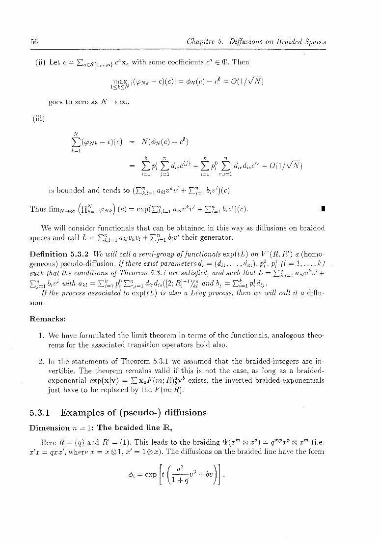
56 Chapitre 5. Diffusions on Braided Spa ces
(ii) Let c = 2:aES{1, ... ,n} caxa with sorne coefficients ca E Œ. Then
(iii)
max /('PNk - t)(c)/ = 4>N(C) - c0 = O(ljv'N) 1~k~N
goes to zero as N -+ 00.
N
I)'PNk - t)(c) k=1
k n k n
LP; Ldijc{j} + LP? L dirdisCrs + O(ljv'N) i=1 j=1 i=1 r,s=1
is bounded and tends to (2:k,l=l aklvkvl + 2:5=1 bivi)(C).
Thus limN~oo (TIf=l 'PNk) (c) = exp(2:k,l=l ak/vkvl + 2:5=1 bivi)(C). • We will consider functionals that can be obtained in this way as diffusions on braided
spaces and call L = 2:k,I=1 aklVkVI + 2:j=l bivi their generator.
Definition 5.3.2 We will call a semi-group of functionals exp( tL) on V"( R, R') a (homogeneous) pseudo-diffusion, if there exist parameters di = (di1 , ... , din ), p?, PT (i = l, ... , k) such that the conditions of Theorem 5.3.1 are satisfied, and such that L = 2:k,l=l aklvkvl + 2:j=l bivi with akl = 2:7=1 p? 2:~,s=l dirdis ([2; Rtl )kÎ and bj = 2:7=1 pt dij .
If the process associated to exp( tL) is also a Lévy process, then we will cal! it a diffuSIOn.
Remarks:
1. We have formulated the limit theorem in terms of the functionals, analogous theorems for the associated transition operators hold also.
2. In the statements of Theorem 5.3.1 we assumed that the braided-integers are invertible. The theorem remains valid if this is not the case, as long as a braidedexponential exp(x/v) = 2:xaF(m; R)ïyb exists, the inverted braided-exponentials just have to be replaced by the F(m; R).
5.3.1 Examples of (pseudo-) diffusions
Dimension n = 1: The braided line IRq
Here R = (q) and g = (1). This leads to the brai ding \l1(xm Q9 xP ) = qmp xp Q9 xm (i.e. x' x = qxx', where x = x Q9 l, x' = 1 Q9 x). The diffusions on the braided line have the form

5.3. A construction oI( pseudo-) diffusions on braided spaces 57
Using the expansion e-tu2/2+xu = I:~o ;~ Hp(x, t) with the Hermitepolynomials Hp(x, t) =
"Π( p ) (2k)! p-2k( t)k fi d r th t i...Jk=O 2k 2kk! x - we n lor e momen s
Dimension n = 2: The quantum plane Œ~IO
Here
(
q2 0 0
R = 0 q q2 - 1 o 0 q o 0 0
R' = q-2 R.
This is the standard two-dimensional quantum plane. It has two generators X, y with relations yx = qxy and braid statistics x'x = q'2xx' , x'y = qyx' , y'y = q2yy', y'x = qxy' + (q2 - 1 )yx'. For the second braided-integer we get
(
1 + q2 0 0
"[2' R] = 0 1 q , 0 q q2
o 0 0
o ) o o .
1 + q2
i.e. it is not invertible. There exists nonetheless a braided-exponential [Maj96, Example 5.4]
xava 00 (x. v)p exp(xlv) = L [1' 2]' = L [ . -211'
aES{l, ... ,n} al, q. p=O P, q "
where lm; q2] = 1;::;;; and [mi q2]! = n:'=l [f..l; q2J. For the generator we get
The free braided-space
Here R' = P, there are no relations in the alge bras V (R, R') and V' (R, R') since the ideal generated by R~2V2Vl = VIV2 (respectively xlx2R~2 = x2xd is equal to {O}, i.e. we have the free algebra with n generators. {va;a E S{l, ... ,n}} (respectively {xa;a E
S{l, ... ) n}}) is thus· a basis of V(R, R') (respectively V'(R, R')). VVe will assume that R is also equal to P, i.e. that the braiding is given by \If (vi ®
vj) = (vi ® vJ) (respectively \If(x; ® Xj) = (Xi ® Xj)). In this case the braided-integers lm; P]b = m6a b, m = lai = Ibl, are invertible and thus

58 Chapitre 5. Diffusions on Braided Spa ces
The dual action is if al = i, else
on the basis elements. Generators of diffusions have again the form
n n
L = L aklokol + L bjoj k,l=l j=l
with symmetric akl.
5.3.2 Examples of true diffusions
A free two-dimensional braided plane: V' = IRq * IRq
(5.4)
The algebra underlying this ex ample can be considered as the free product of the braided line with its dual. As an algebra it is the free unital algebra ([; < x,p> with two generators. Let x be the generator of the braided-covector spaceIRq, and p that of the braided-vector space dual to it (i.e. another copy of IRq). Let q E IR\{O}, so that R = (q) is of real type 1 in the sense of [Maj95a]. Following Majid's definitions we have the braid relations
and
*lRqS2,lRq
* lRq S2,lRq S2,lRq S2,lRq
1 X X = qxx 1 -1 1 X P = q px
p'X = q-1xp' 1 1 pp = qpp,
IRq0IRq ~ IRq0lRq, x* = p
IRq0~0IRq0~ ~ IRq0~0IRq0~, x* = p', (X't = p,
turn IRq0IRq and IRq0~0IRq0IRq in into *-algebras such that .6. : IRq0IRq ~ IRq o IRq o IRq o IRq satisfies .6. 0 *lR 0lR = *lR 0lR 0lR 0lR 0 r 0 .6.. Even though this *-structure does not suit
q- q q- q- q- q
our purposes, at least not in this form, it does tell how we can guess a 'better' one. The coproduct on IRq and its dual extends to a map .6.0 : IRq * IRq ~ (IRq o IRq ) *
(IRq0IRq) = ([; < p,p',x,x' > l'IQ, where'IQ is the ideal generated by x'x - qxx' and p' p - qpp', and satisfies .6. 0 *lRq*lRq = * (lRqS2,lRq )*(lRqS2,lRq ) 0 .6., if we define the * -structures in those algebras by
*lRq*lRq
* (lRqS2,lRq)* (lRqS2,lRq)
IRq * IRq ~ IRq * IRq, (IRq0IRq) * (~0IRq) ~ (IRq0IRq) * (IRq0IRq),
x* = p,
x* = p', (x')* = p.
We now note that we get (IRq*lRq)0(IRq*~) ifwe quotient by the relations qxp = px and qp' x' = x' p', i.e. (IRq * ~ )0(IRq * IRq ) = (IRq o IRq ) * (~0IRq) 1 {qxp = pxp, qp' x' = x' p'} = ([; < p', X,p, x' > II, where l is the ideal generated by x'x - qxx' , .qxp - px, qp'x' - x'p', and p' p - qpp'. The canonical projection 7r : (IRq o IRq ) * (IRq0IRq ~ (IRq * IRq )0(IRq * IRq) is a * -algebra homomorphism, and .6. = 7r 0 ~ turns V· = IRq * IRq into a braided * -Hopf algebra in the sense we need. In particular, the coproduct is a *-algebra homomorphism.

5.3. A construction of (pseudo-) diffusions on braided spaces 59
Note that we now have Pl = p' and Xl = X in the first factor of the tensor product, and P2 = P and X2 = x' in the second, i.e. the braid relations take the form
and the *-structure becomes xi = pi, i = L 2. The braiding of the real line, and thus also that of V', are induced by an action and
coaction of the group algebra Œ7l. ~i' is the (free) braided plane associated to the matrices
( q 0 0 0 )
R = 0 q-l 0 0 . 0 0 q 0
o 0 0 q-l
The possible generators of pseudo-diffusions are of the same form as in Equation (,5.4), but now we are interested in generators of 'true' diffusions, i.e. W-invariant, hermitian, conditionally positive generators. Choose the set of all words {l = 0, x, p, xx, :rp, px, pp, ... } as basis of V", then rpxp and Opx \\'i th
if 11 = ;T:P, eise,
ifu=]KC, else,
on basis elements 11 are such generators. The processes associated to these generators have been studied by lvI. Schürmann[Sch93], we find the processes that have the Azéma martingales as classical version.
Let us now consider an example whose braiding do es not come from a group, but from a non-commutative and non-cocommutative bialgebra.
Diffusions on the four-dimensional braided-covector space V' = Œ~IO * Œ~IO
Let again q in IR\{O}, and set V' = Œ~lo *Œ:10 = Œ < v, w, x, y> / {yx - qxy, vw - qwv}. A similar construction as in the preceding example leads to a four-dimensional braidedcovector space, where the braid relations between Xl, YI and X2, Y2 are described by the R-matrix of the braided plane,
(
q2 0
R= a q a 0 a a
o q2 -1
q o
those between Xl, YI and V2, W2 by its second inverse,

60 Chapitre 5. Diffusions on Braided Spa ces
those between VI, Wz and Xz, Yz again by R, and, finally, those between V2, W2 by R- 1 ,
see also subsection 5.2.3. The *-structure is defined by x* = V and y* = w, compare also [Maj95a].
{xnym ln, m E IN} and {wmvn ln, m E IN} are bases of the two components of the free product defining vv, and therefore we can take the finite, alternating sequences of elements of these bases as a basis of V·: {l = rh xnlyml wm1vn1 xnl yml.wm2 "n2 u,mlvnlxn2ym2 ln 17, m . m VJ, , j v , j'" 1, 2,···, 1, '2,··· The functional defined on this basis by
generates a diffusion.
5.4 Appell systenlS
if u = xv,yw else,
Appell systems {h k ; k E IN} can be defined by the conditions
Al: hk is a polynomial of degree k,
E IN}.
where D = dl d:r. Examples are furnished by shifted moment sequences of the form
where p is any probahility measure on IR with aIl moments finite. For example in the Gaussian case this gives the Hermite polynomials Hn(x) = vk J1R(x + iyte-y2/2dy. Recently
analogous classes of 'moment polynomials' on Lie groups [FS92] and quantum groups [FFS95] have been introduced. They cease to he polynomials in general.
The definition on quantum groups is easily adapted to braided groups.
Definition 5.4.1 We define the Appel! polynomials on the braided covector space V·(R, R') with respect to the funciional <P by
ha = (cP ® id) 0 i).xa ,
i.e. ha = T,p(xa), for a E S{l, ... ,n}.
vVe are in particular interested in the Appell systems with respect to diffusions.
Proposition 5.4.2 Let cPt be a diffusion on V·(R, R') with generatoT Land {ha(t); a E S{l, ... , n}} the associated Appell system. Then we have the following:
1. ha(t) = X a + Pa(t), where Pa(t) E EB~~~l V·(R, R,)(a))
2. Diha = I:bESlal-1{l, ... ,n}[lal; Rl~·bhb, where Di = exp(tL)éJi exp( -iL) and i.b the concatenation of i with h, i.e. i.b = ib1 ... blal - l ,

5.4. Appel! systems
3. the ha (t) satisfy the evolulion equation atu = Lu.
Proof: Note that 1. and 2. are the analogues of Al and A2.
1. The braided-binomial theorem [Maj96, Equation (91)] tells us that
lai < [lai ]b.C .6xa = L L . ; R Xb ® XC'
i=O bESi{l, .... n},cESlal-i{l, ... ,n} l a
where the braided-binomial coefficients are defined by
[ ~; R]
[ ~ ; R]
[ ~ ;R]
[m-1 ] [m-1 ] (P R)r,r+l ... (P R)m-l,m l' _ 1 ; R + l' ; R ,
1,
= 0 for l' > m.
61
Note that this formula can also be used to calculate the Appell systems, if the moments of the process are known.
2.
3.
D' ha exp( lL )fi exp( -tL) exp( tL )Xa
with [Maj96, Equation (77)].
exp(tL)éixa
exp(tL) L bESlal-! {l, ... ,n}
rial' R]i.bx l'a b
L [la!; R]~bhb bESlal-! {l, ... ,n}
at exp( tL )xa = L exp( tL )xa
Lha(t).
Il Property 2 shows that the Di act as lowering operators. We also define raising operators.
Proposition 5.4.3 Let)( = exp(tL)Xiexp(-tL)) then

62 Chapitre 5. Diffusions on Braided Spaces
Examples
5.4.1 The braided line 1Rq
The Appell polynomials associated to the functional <Pt = exp(tL) where L = l~q v2+bv are
These polynomials are solutions of
with u(x, t = 0) = xk (where J is the q-difference operator (Jf)(x) = f(~(~={jx»).
For b = 0, a = J(1 + q)/2 the Appell polynomials simplify to
[~l [k; q]!t llxk-2zi hk(x;t) = L [k _ 2 . ]I211 l' lI=O V, q. v.
these polynomials are a q-analogue of the Hermite polynomials (see also [FFS95]).
5.4.2 The quantum plane Œ;Io
We choose <Pt = exp tL with L = l:q2 (ai + ai). We get
<P = ~ tr ~ [ r . -4] a211 a2(r-1I) t L..t (1 + q2)rr! L..t V' q 2 l
r=O lI=O
since a2al = q- I ala2. This leads to the following formula for the Appell polynomials:
- hrm(x,y;t) = exp(tL)xrym
[fl [Tl [ Il ~ v ; q-4] lm; q2]![r; q2]!q2~(r-211) t~+lI ~ ~ [m - 21l - 1; q2]![r - 2v - 1; q2]!(1 + q2)~+1I(1l + v)! xr-211ym-2~,
where [ : ; q-4] are the braided-binomial coefficients with respect to R = (q-4) E M(l)®
M(l). These polynomials solve the evolution equation
1 (2 2) atU = --2 al + O2 U l+q
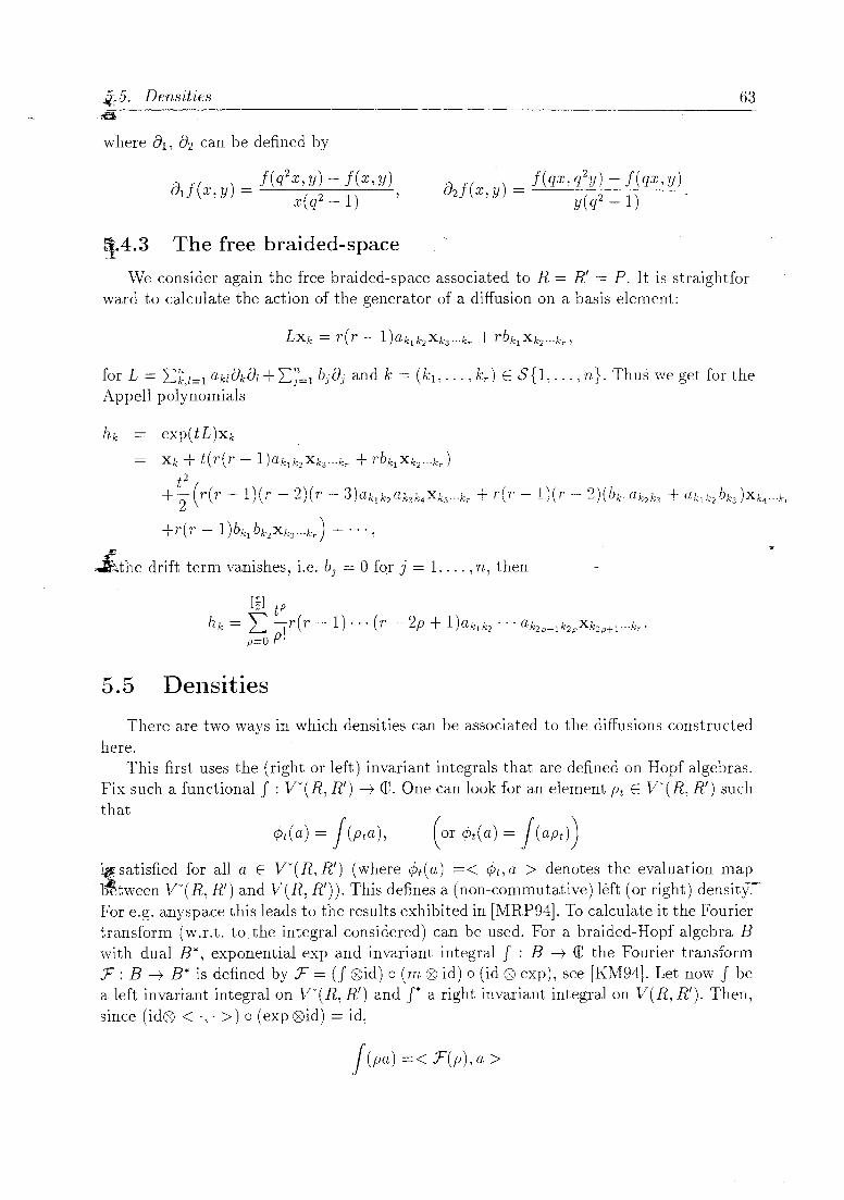
~15. Densities 63 -:e
where fA, 82 can be defined by
8 f( ) = f(q 2x, y) - f(x, y) 1 X,y x(q2-1) '
o::l f( .) = f(qx,q2y) - f(qx,y) U2 X, Y (2)' Y q -1
~.4.3 The free btaided-space
We consider again the free braided-space associated to R = R' = P. It is straightforward to calculate the action of the generator of a diffusion on a basis element:
for L = I:k,l=l aklokol + I:7=1 bjoj and k = (k l , ... , kr ) E S {1, ... , n}. Thus we get for the Appell polynomials
hk exp(tL)Xk
Xk + t( r( r - 1 )ak1 k2 Xk3 .··kT + r'bk1 Xk2 , .. kT)
t2 . 1 • ___ (~(~ _ l\1.,... - ·)Î(". - '1În, , n, , y, , -+ r{r - l)(r - '))(b, rl l ' + '1' , b )X
T 2 \.' \' J-J\' i.,..IJ\' Vj UlK IK:2'""K:3K:4 ...... ,I\;S···K r l '\' -/\" ~/\ t;;' l U"r{21;3 ' UlCilZ2 k2.! ,1.;4. ... ,l;:.(
+r(1' - 1 )bk1 bk2Xk3 "'kT) + ... ,
~the drift term vanishes, i.e. bj = 0 for j = 1, ... ,n, then
5.5 Densities
There are two ways in which densities can be associated to the diffusions constructed here.
This first uses the (right or left) invariant integrals that are defined on Hopf algebras. Fix such a functional J : V-(R, R') ~ œ. One can look for an element Pt E V-(R, R') such that
~satisfied for an a E,r(R,R') (where qyt(a) =< cDt,a > denotes the evaluation map 'l~tween V-( R, R') and V( R, R')). This defines a (non-commutative) left (or right) density.For e.g. anyspace this leads to the results exhibited in [MRP94J. To ca.lculate it the Fourier transform (w.r.t. tO,the integral considered) can be used. For a braided-Hopf algebra B \Vith dual B*, exponential exp and invariant integral J : B ~ œ the Fourier transform F: B ~ B* is defined by F = (J ®id) 0 (m ® id) 0 (id ® exp), see [KM94]. Let now J be a left invariant integral on V- (R, R') and r a right invariant integral on V (R, R'). Then, since (id® < ',' » 0 (exp ®id) = id,
!(pa) =< F(p),a >

64 Chapitre 5. Diffusions on Braided Spa ces
for all a E V~(R, R') and p E V(R, R'). Thus we need to invert the Fourier transform F to find the density corresponding to the functional (Pt. By [KM94, Proposition 6.4], F* 0 F = vol S, where vol is a constant andF* the Fourier transform W.r.t. 1*, i.e. F* = (id 0 1* om) 0 (\li 0 id) 0 (id o exp). Thus
1 -1 Pt = -1 S 0 :F* ( CPt).
vo
Take, e.g., the braided-line and CPt = exp( t~2). We shall use the Jackson integral J!":;': f( x )dqx where Î is a parameter. For-f(x)='Efnxn we set- fb) = EfnÎn and-
if the right-hand-side converges. We will express the density in terms of the dis crete qHermite II polynomials
_ n [~l (_1)kq-2nkqk(2k+l}xn-2k hn( x; q) = (1 - q) ln; q]! E (1 _ q2)k[k; q2]!(1 _ q)n-2k[n - 2k; q]!'
With the orthogonality relations for the discrete q-Hermite II polynomials [Ko095, Equation (8.14)] and
we get
where eq2(z) = L~=o [n~;2l!' and cq(1) is a constant depending only on q and Î (for its value see [Ko095, Equation (8.15)]).
The other way, commonly used in quantum probability (see e.g. [Mey93]) leads to a density on the usual real line. Consider for example a diffusion CPt = exp(tv2/2) on the braided line, and the generator x, then CPt ( eitx ) can be interpreted as the Fourier transform of the density of x in the state CPt. Let 0 < q < 1 and Y = (1 - q) E~o Xi, where the Xi are independent, and exponentially distributed with respective means qi
(see [Fei87]). Then E(eiuY ) = I1~o(1-iu(1-q)qirl = E~=o(iu)n/[n;q]! = e~u. Thus cpt(E(eiuYx )) = CPt(e~ux) = e-tu2/2, and it follows that Yx has a Gauss distribution. This determines the distribution of x uniquely, see [Fei87, Theorem 3].
5.6 Conclusion
The notion of q-Brownian motion introduced by Majid is extended in this paper to braided spaces. The resulting pro cesses differ from the ones obtained in [BS91, MM93]

5.6. Conclusion 6.5
by more algebraic considerations. To obtain these (for fixed parameter t=l, say), we can consider the semi-direct cross product of the braided li ne with its dual. This algebra has basis {vn 0 xm; n, mE lN} and the defining relations are vx - qxv = 1 (where v = v 0 1, x = 10 x). Take the functional cP defined by cP(r:, anm vn xm) = aaa, then the distribution of x + v in the state cP is equal to that of [BS91] for t = 1, for a study of its density see [LM95]. This density is concentrated on the bounded interval [-1/ y1=q, 2/ vr=q] (for -1 < q < 1). The q-deformed Brownian motion of [MM93] can be obtained similarly. Obviously, there is still sorne more non-trivial construction required to pass from the random variable presented here to the full process.

66 Chapitre 5. Diffusions on Braided Spa ces

Chapitre 6
Gauss Laws in the Sense of Bernstein and U niqueness of Embedding into
Convolution Semigroups on Quantum Groups and Braided Groups
Uwe Franz Daniel N euenschwander 7 René Schott 8
Résumé
The goal of this paper is to characterise certain probability laws on a class of quantum groups or braided groups that we will call nilpotent. First we introduce a braided analogue of the Heisenberg-Weyl group, which shaH serve as standard example. 'vVe introduce Gaussian functionals on quantum groups or braided groups as functionals that satisfy an analogue of the Bernstein property, i.e. that the sum and difference of independent random variables are also independent. The corresponding functionals on the braided line, braided plane and a braided q-Heisenberg-Weyl group are determined. Section 6.5 deals with continuous convolution semigroups on nilpotent quantum groups and braided groups. We extend recent results proving the uniqueness of the embedding of an infini tel y divisible probability law into a continuous convolution semigroup for sim ply connected nilpotent Lie groups to nilpotent quantum groups and braided groups. Finally, in Section 6.6 we give sorne indications how the semigroup approach of Heyer and Hazod to the Bernstein theorem on groups can be extended to quantum groups and braided groups.
Accepté pour publication dans Probability Theory and Related Fields
ï. Université de Lausanne, École des Hautes Études Commerciales, Institut de Sciences Actuarielles, CH-1015 Lausanne, Switzerland, Email: [email protected]
8. CRIN-CNRS, BP 239, Université H. Poincaré-Nancy 1, F-54506 Vandœuvre-lès-Nancy, France, Email: [email protected]
67

68 Chapitre 6. Gauss Laws in the Sense of Bernstein on Quantum Groups

6.1. Introduction 69
6.1 Introduction
Quantum probability is now a quite active research area motivated by applications in physics. Recent books of Biane [Bia93], Meyer [Mey93L and Parthasarathy [Par92] are recommended as introductions to this field. For quantum probability on Hopf algebras see Majid [Maj95b] and Schürmann [Sch93]. In this paper we continue the investigation of probability measures on quantum groups and braided groups initiated in [FFS97, FS96b]. Our goal is to characterise certain probability laws on a class of quantum groups or braided groups that we will caIl nilpotent. \Ve determine the functionals on these structures which satisfy an analogue of the Bernstein property, i.e. that the sum and difference of independent random variables are also independent. In doing so we extend results obtained previouslyon Lie groups by D. Neuenschwander et al., cf. [Neu93, NRS96, NRS97]. Then we turn to convolution semigroups. We shov./ the uniqueness of embedding into continuous convolution semigroups on nilpotent quantum groups and braided groups, and calculate the generators of continuous convolutions semigroups on several nilpotent braided groups that satisfy an analogue of the Bernstein property.
The organization of the paper is as follows: Section 2 provides some preliminaries on quantum groups and quantum probability. A braided Heisenberg-\Veyl group is introduced in Section 3 and the corresponding Gaussian functionals in the sense of Bernstein are given in Section 4. The embedding problem is investigated in Section 5, while Section 6 gives some hints on Gaussian semigroups in the sense of Bernstein on quantum groups and braided groups. Conclu ding remarks and further research aspects are mentioned in Section 7.
6.2 Preliminaries
6.2.1 Quantum groups
\Ve briefly recall some definitions concerning quantum groups and braided groups, see also [Maj95b] and references therein.
Recall that a quantum group is a Hopf algebra, i.e. an associative unital algebra (H, m, e) with two homomorphisms ~ : H --t H ® H, c : H --t <C, and an antihomomorphism S : H --t H that satisfy
(~® id) 0 ~
(c ® id) 0 ~
m 0 (id ® S) 0 ~
(id ®~) o~,
(id ® c) 0 ~
m 0 (5 ® id) 0 ~ = e 0 c.
These maps are called coproduct, counit, and antipode, respectively. Here the tensor product H ® H is considered as an algebra with the multiplication defined by m0((a iZl b)iZl(c®d)) = ac®bd, i.e. m@ = (miZlm)o(id®TiZlid), where T : HiZlH --t HiZlH is the fiip automorphism, T( a ® b) = b ® a. Placing ourselves in a braided category and substituting T by the brai ding W we are naturally led to braided Hopf algebras or braided groups. The axioms ab ove remain unchanged, but now m, e, D., c, and 5 have to satisfy certain compatibility conditions with respect to the brai ding W. The comultiplication ~ has to

70 Chapitre 6. Gauss Laws in the Sense of Bernstein on Quantum Groups
be an algebra homomorphism from H to H0H, i.e. the algebra structure in the tensor product is defined by mw = (m0m)o(id0w0id), or mw((a0b)®(c®d)) = aW(b®c)d. And the antipode is no longer an anti-homomorphism, but satisfies Som =moWo(S®S).
Example: The braided line IRq. Let q E Œ\ {O}, q not a root of unity. As an algebra IRq is isomorphic to the ring of polynomials in one variable IR[ x J. The braiding used here Îs defined by w(xn 0xm) = qnmxmxn. On the generator the coproduct, counit, and antipode are defined by
6.(x) = x + x', é(X) = 0, S(x) = -x,
where we used x = x 0 1, x' = 1 ® x. From this one computes
~, n(n-l). . and :'(xn) = (_I)n q- 2 - x n. Recall that the q-numbers qn, the q-factonal qn1 and the
q-binomial coefficients [ ~ lare defined as .J q
n n-l v qn - 1 qn = L q = 1 '
v=O q-qn! = il qV)
v=l
Example: The braided plane Œ;lo. Again q E Œ\ {O}, q not a root of unity. The braided plane is the braided Hopf algebra with two generators x, y and defining relations
yx qxy,
XiX = q2xx' ,
y'x = qxy' + (l- l)yx',
6.x = x + x',
é(X) = é(Y) = 0,
1 1 X Y = qyx,
ly = q2yyl,
tly = y + yi
S(x) = -x, S(y) = -y
vVe will present another example of a braided group in Section 6.3.
6.2.2 Quantum probability
vVe summarize the basic definitions of quantum probability or non-commutative probability. A quantum probability space is usually defined as a pair (A, <p) consisting of a *-algebra A and a state (i.e. a normalizeded positive linear functional) <P on A. A classical probability space (ft, F, P) gives rise to a quantum probability space by taking a *-algebra of complex-valued integrable functions on ft, e.g. Loo (ft, F, P), and the functional defined by <P : f f-7 In fdP.
A quantum random variable j over a quantum probability space (A, <p) on a *-algebra B is simply a * -algebra homomorphism j : B --+ A. A classical random variable X : ft --+ E ovel' a probability space (ft, F, P) with values in a measurable space (E, f) defines a quantum l'andom variable via jx(J) = foX for f E B (where B is an appl'opl'iately

6.3. A braided Heisenberg- Weyl group 71
chosen algebra of functions on E). For a quantum random variable j : B ---t A we will caH cpj = <I> 0 j its distribution in the state <I>.
In this article we will often use the terminology introduced above but neglect the *structure. The reason for this is that the algebras we consider have natural * -structures on1y for rather special values of the parameters. Vve will for example characterize Gaussian functionals in the sense of Bernstein using on1y their algebraic properties. Once this is done one can without much difficulty check positivity for those cases where a natural * -structure is defined.
6.3 A braided Heisenberg-Weyl group
In this section we introduce a braided Hopf algebra structure for the q-oscillator algebra HW q defined by
ac - qca = (1 - q)b, ab = ba, cb = bc, (6.1 )
where q E Œ\ {O}, q not a root of unity. For other quantum or braided groups related to the Heisenberg group see [BM93] and the references therein.
\Ve can also regard this algebra as generated by two generators a. c with the cubic relations
aac + qcaa
acc + qcca
(l+q)aca
(1 + q)cac
with q E Œ, q not a root of unity. If we define the braiding by
a' a = qaa' 1 1 a c = ca 1
c'a = -ac' C'C = qcc' q
then /:::..a = a + a', /:::..c = c + c'
(6.2)
defines an algebra homomorphism from HWq to HWq@HWq. The counit is defined by f(a) = f(C) = 0 (extend as a unital algebra homomorphism). The braided bialgebra defined in this way also admits an antipode. Define S by
S(a) = -a, S(c) = -c,
and extend by Som = m 0 \.II 0 (S @ S). The advantage of introducing a third generator, e.g. by ac-qca = (l-q)b or d = ac-ca,
is that {anbmcr ; n, m, r E lN} and {andmd'; n, m, r E lN} are bases (Poincaré-Birkhoff-Witt bases) of HW q'
One can calculate the coproduct on a general basis element

72 Chapitre 6. Gauss Laws in the Sense of Bernstein on Quantum Groups
We will construct the dual of HW q' The coproduct of HW q defines an algebra structure in its dual. Let X, Y : HW q -+ œ be two functionals on HW q, then their pro du ct is defined by
where we used Sweedler's notation, ~(u) = L U(I) Q9 U(2). For the functionals defined by
we see that they span an algebra, denoteà by HW~, generated by the three elements
x = X lOO , y = X OlO , Z = X 001 such that X ijk = Z~yJIXII and , qk .q)"q •.
xy = qyx, yz = qzy, xz - zx = y.
We see that this algebra is isomorphic to HWq , the isomorphism being x f--t a, Z f--t c. The following formula is useful to compute products of general basis elements of the
HvV q algebra, it can be derived by induction.
rAn (0 -1) '( -1') î(' l)k r n _ "" q r,' q n· - n-kdk r-k
C a - ~' 1) '( 1) '( 1) ra C. k=O (q- r-k· q- n-k· q- k·
If q is real, then the involution * : HW q -+ HW q defined by
satisfies
*0*
*om
a* = c, b* = b, * c = a.
id (i.e. (a*)* = a Va E A),
o E,
* 0 S,
i.e. * is an anti-homomorphism,
(6.4)
i.e. turns HWq into a braided *-Hopf algebra. For the origin of the last three conditions see e.g. [Maj95a].
6.4 Gaussian functionals in the sense of Bernstein
The Gauss law plays a central role in probability theory on Euclidean spaces. Bernstein's theorem gives a characterisation in terms of the group law of the underlying space.
Theorem 6.4.1 Let P be a probability measure on IRn. P is a Gauss law if and only if for aU pairs of independent random variables X, Y with distribution P the random variables X + Y and X - Y are a/so independent.

6.4. Gaussian functionals in the sense of Bernstein 73
We want to remark here that it is not essential that the two random variables X and y have the same law, we also have the following version of the above theorem.
Theorem 6.4.2 Let Px and Py be two probability measureson IRn . If there exists a pair of independent random variables XJ y with distribution Px, Py , respectively, such that the random variables X + Y and X - Y are also independent, then Px and Py are Gauss laws (with identical covariance matrices).
This characterisation can be used as a definition of Gaussian functionals on groups in general, if sorne care is taken concerning the order of the factors in non-commutative groups.
Definition 6.4.3 Let G be a (locally compact topological) gmup. A probability measure fi on G is called Gaussian in the sense of Bern.stein if there exists a probability spa ce (0, B, P) and a pair ofG-valued r.v. X, Y, su ch that fi = X(P) = Y(P), and (X· Y, Y ·X) and (X . y-l, y-l . X) are independent.
D. Neuenschwander showed recently [Neu93] that the Gauss measures in the sense of Bernstein on the Heisenberg-vVeyl group are exactly the Gauss measures concentrated on Abelian subspaces. In fact, this result holds on connected simply-connected nilpotent Lie groups in general [NRS96, NRS97].
vVe will now give a definition of Gaussian functionals on (braided) Hopf algebras"
6.4.1 Definition of Gaussian functionals in the sense of Bernstein on (braided) Hopf algebras
We have to translate X + Y and X - Y into Hopf algebra language. Replacing the group operation by the coproduct and the inverse by the antipode we write )1 *)2 = mA 0 U1 0 )"2) 0.6..[3 and )1 * ()2 05) = mA 0 ()1 0 ()2 0 5)) 0 .6..[3 for the sum and difference of two quantum random variables )1,)2 : B --t A, see also [AS\V88, Sch93).
Definition 6.4.4 A functional y on the (bmided) Hopf algebra B is called right (left) Gaussian in the sense of Bernstein if there exists a quantum probability space (A, <J») and two independent quantum random variables )1,)2 : B --t A such that y = <J) 0)1 = <J) 0 )2 and the applications
J = mA 0 U1 0 )2) 0.6..[3
(J = mA 0 (jl 0 )2) 0 .6..[3
and I{r = mA 0 (jl 0 )2) 0 (id ® 5) 0.6..[3
and KI = mA 0 U1 0 )2) 0 (50 id) 0.6..[3)
form also a pair of independent quantum random variables. A Gaussian functional in the sense of Bernsteinis a functional that is right and left
Gaussian in the sense of Bern.stein.
Here)l and)2 are required to have the same law. We shaH see that in the examples we consider this condition is too strong. We propose therefore also a weaker definition that is motivated by Theorem 6.4.2.
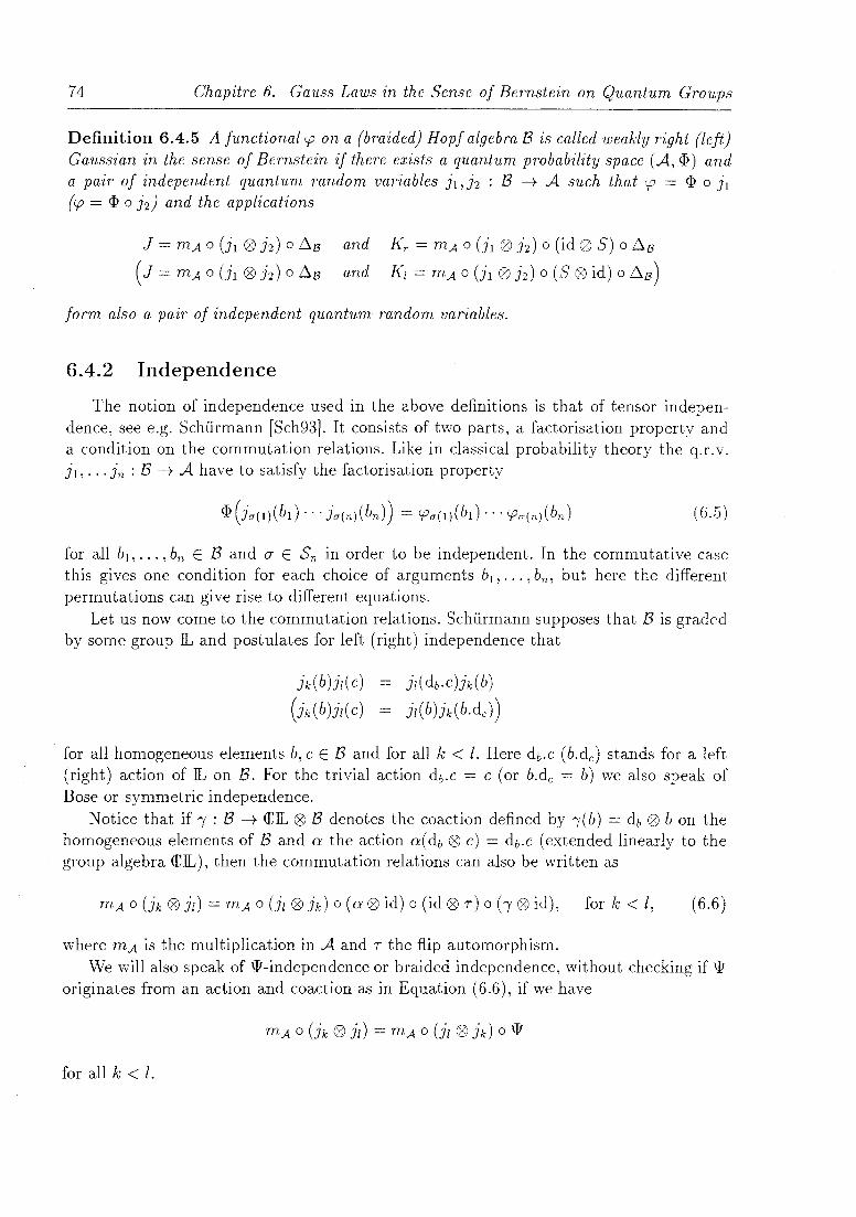
74 Chapitre 6. Gauss Laws in the Sense of Bernstein on Quantum Groups
Definition 6.4.5 A functional rp on a (braided) Hopf algebra B is called weakly right (left) Gaussian in the sense of Bernstein if there exists a quantum probability space (A, <P) and a pair of independent quantum random variables jl, j2 : B -7 A such that rp = <P 0 jl (rp = <P 0 j2) and the applications
J = mA 0 (il @ j2) 0 ~B
(J = mA 0 (il @ j2) 0 ~B and Kr = mA 0 (il @ j2) 0 (id @ S) 0 ~B
and Kt = mA 0 (il @j2) 0 (S@id) 0 ~B)
form also a pair of independent quantum- random variables.
6.4.2 Independence
The notion of independence used in the ab ove definitions is that of tensor independence, see e.g. Schürmann [Sch93J. It consists of two parts, a factorisation property and a condition on the commutation relations. Like in classical probability theory the q.r.v. jl, ... jn : B -7 A have to satisfy the factorisation property
(6.5)
for aIl bl , ... ,bn E Band (7 E Sn in or der to be independent. In the commutative case this gives one condition for each choice of arguments bl , ... , bn , but here the different permutations can give rise to different equations.
Let us now come to the commutation relations. Schürmann supposes that B is graded by sorne group IL and postulates for left (right) independence that
jk(b)jt(c)
(jk(b)jl(C)
j[(db.c)jk(b)
jt(b )jk(b.dc))
for aIl homogeneous elements b, cE B and for all k < l. Here db.c (b.dc ) stands for a left (right) action of IL on B. For the trivial action db.c = c (or b.dc = b) we also speak of Bose or symmetric independence.
Notice that if, : B -7 œIL @ B denotes the coaction defined by ,(b) = db @ b on the homogeneous elements of B and a the action a( db @ c) = db.c (extended linearly to the group algebra œIL), then the commutation relations can also be written as
mA 0 (ik @jl) = mA 0 (il @jk) 0 (a @ id) 0 (id @ r) 0 b @ id), for k < l, (6.6)
where mA is the multiplication in A and r the fiip automorphism. We will also speak of 'lI-independence or braided independence, without checking if 'li
originates from an action and coaction as in Equation (6.6), if we have
for aIl k < 1.

6.{ Gaussian functionals in the sense of Bernstein 75
6.4.3 Preliminary results
Before presenting explicit results on particular (braided) Hopf algebras, we give a lemma showing a link between left and right (weakly) Gaussian functionals in the sense of Bernstein.
Taking a Hopf algebra H whose antipode S is invertible, we can define three Hopf algebras HOP, HCop, HOPcop, if we replace the multiplication or the comultiplication by their opposites m OP = mOT or 6 cop = T 0 6, and invert the antipode each time we take an opposite. Similarly, we can take opposites or co-opposites of braided Hopf algebras using the braiding or its inverse and inverting the braiding, i.e. the opposites lie in the braided category that has the opposite brai ding \jf-l.
In particular, let (B, m, L 6, E, S, \jf) be a braided Hopf algebra with invertible antipode, and define 6 cop = \jf-l 0 6. Then BCop = (B, m, 1, 6 cop , E, S-I, \jf-l) is also a braided Hopf algebra [Maj93a, Lemma 4.6]. Notice that we have to use the inverse of the braiding, A cop = \jf 0 6. does not le ad to a braided Hopf algebra. vVe can also define a braided Hopf algebra with opposite multiplication. Set m OP = m 0 \jf-1, then BOP = (B, m OP , 1,.6.., f, S-l, \jf-l) is a braided Hopf algebra. Combining the above operations we get the braided Hopf algebras (BcoptP = (B, m 0 \jf, 1, \jf-l 06, E, 5, \jf) and (BoptOP = (B lT,-1 1 .TI ;\ ç C .T') d 0' Il Bkxcopop - (·B .TrAc 1 .T,-Ac - C .Tl) ,m 0 'l' ,,'l' 0 Ll., '-', U, 'l' ,an , more ('Jenera y, -, rn 0 'l' , ,'l' ,c, ,.-i, 'l'
for k E 'll .. AH these braided Hopf algebras are isomorphic, since the antipode is an isomorphism from Bkxcopop to B(k+1)xcopoP. In the same way we can construct a chain of isomorphic braided Hopf algebras starting from BOP or BCOP, in particular, 5 : BOP --t BCop
is an isomorphism. vVe have the following lemma.
Lemma 6.4.6 Let jl, j2 : B --t A be a pair of \jf -independent quantum random va7'iables on B over some quantum probability space (A, <p). Then the following statements are equivalent.
1. j(jl,j2) = mAo(jl(2)j2)o6 and K r (jl,j2) = mAo(jl@(j20S))o.6.. are independent (and thus cp = <Pojl is a (weakly) right Gaussian functional in the sense of Bernstein
on B),
2. jcoP(j2, jd = mA 0 (j2 (2) jr) 06 cop and KtOP(j2, jr) = mA 0 ((j2 0 S) jd 0 6 cop are independent,
3. jOP(j2 0 S,jl 0 S) = mA 0 ((j2 0 S) (2) (jl 0 S)) 0 6 and K~P(j2 0 S,jl 0 S) = mA 0
((j2 0 SoS) (2) (j1 0 S)) 0 6 are independent.
Pro of: The equivalence of 2. and 3. is clear since S : BOP --t BCop is an isomorphism. Let us show now that 1. and 2. are equivalent. The pair (jl,j2) is \jf-independent if
and only if (j2,jr) is \jf-l-independent. vVe find
j(jl,j2) mA 0 (jI @ j2) 0 6.
- mA 0 (jl (2) j2) 0 \jf 0 \jf-l.6..
mA 0 (j2 (2) jd o6coP
j COP(' ') )2, JI ,

76
and
Chapitre 6. Gauss Laws in the Sense of Bernstein on Quantum Groups
mA 0 (j1 ® (j2 0 S)) 0 ~
mA 0 ((j2 0 S) ® )1) 0 ~cop
KtOP(j2,)d,
so that J(j1,)2) and K r (jt,)2) are independent exactly wh en JcoP(j2,)d and K/coP(j2,)d are independent. Ô
To use this lemma to relate (weakly) left Gaussian functionals in the sense of Bernstein to (weakly) right Gaussian functionaIs in the sense of Bernstein on the opposite or coopposite quantum/braided group we have to deal with two technical difficulties. First, we have to assume that )1,)2 are W-independent. In the examples considered we see that the condition that )1 * )2 is also an algebra homomorphism is sufficient to show that )1,)2 satisfy the commutation relations for W-independence.
Second, in the definition of K~P, KtOP we have the original antipode. We should use the antipode of the opposite or co-opposite quantum/braided group though, i.e. 5- 1 . But in the applications we will see that the condition that )1 *(j205) is an algebra homomorphism implies that there is no difference between )2 0 5 and )2 0 5-1 .
6.4.4 The braided li ne
If we look for left or right Gaussian functionals in the sense of Bernstein on the braided line ffig we find only the trivial solution <p = é (the counit). But, as the following theorem shows, we can find non-trivial weakly Gaussian functionals in the sense of Bernstein.
Theorem 6.4.7 Let <p be a weakly right Gaussian functional in the sense of Bernstein on the braided line IRq, q =1= 0,1, and q not a root of unity. Then there exists a constant a E Πsuch that <p is given by
<p(xn) = an.
Converse/y, if <p is of this form, then it is a weakly right Gaussian functional in the sense of Bernstein.
Proof: We shall determine the pairs of functionals (<p, 'IjJ) on IRq such that there exists a quantum probability space (A, <I» and independent quantum random variables )1,)2 : ffig --7 A such that <p = <I> 0)1 and 'IjJ = <I> 0)2 and the applications
J = mA 0 (j1 ® )2) 0 ~lRq and Kr = mA 0 (j1 ® )2) 0 (id ® S) 0 ~lRq (6.7)
form a pair of independent quantum random variables. This way we will also see that there are no right Gaussian functionals in the sense of Bernstein.
Step 1. We can assume that A is of the form ffig0IRq/{(X')2 = O} = Œ« x, x' » /{x'x = qxx',(x')2 = O}, where Œ« x,x'» denotes the free complex algebra with two generators.
Lemma 6.4.8 Suppose we are given an algebra C and two algebra homomorphisms k1 , k2 : ffig --7 C such that k1 -* k2 and k1 * (k2 0 5) are also algebra homomorphisms. Then there exists an algebra homomorphism 7r : ffig0IRq/{(x')2 = O} --7 C and )1,)2 : ffig --7
ffig0ffig/{(X')2 = O} with)l(X) = x, )2(X) = x', and k i = 7rO)i, i = 1,2.
6.4. Gaussian fundionals in the sense of Bernstein il
Proof of Lemma. Set 7I(x) = kl(X) and 7I(x') = k2(x). We can directly check the relations to verify that 71 is an algebra homomorphism. 7I(x')7I(x) = q7l(x)7I(x') follows sinee k1 * k2 is an algebra homomorphism:
o kl*k2(X2)_(kl*k2(X))2
7I(x)2 + (1 + q)7I(x)7I(x') + 71(X')2 - (7I(x) + rr(x')?
qrr(x)rr(x') - rr(x')rr(x),
Similarly, checking on x2 = x . x that k1 * (k2 0 S) is an algebra homomorphism yields rr(x')2 = O.
Step 2. If <l> is a functional on IRq®IRq/ {( X')2 = O} such that]1 and]2 are independent, then <l> is of the form zp 161 'IjJ, zp : IRq -t Œ, ?jJ : IRq/{(X')2 = O} -t Œ.
This follows from the factorisation property
(where y, z E IRq, a E 52), i.e. taking (J" = id we can set zp = <l>O]I,~' = <l>0]2. FUrthermore, setting y = x and z = xn we see
<l>(j2(X)]I(Xn)) = <l>(X'Xn) = qn<l>(X"X')
qn'IjJ(X)zp(X").
Sinee we suppose that q is not a root of unit y this means zp(x") = 0 for all n 2 l if 'IjJ(x) =f- 1. Viee versa, if zp(xn) =f- 0 for sorne n 2 1, then <l'(x) = O.
Step 3. The only pair (ZP, 'IjJ) such that J = ]1 *]2 and Kr = ]1 *(j2 0 S) are independent is zp as given in Theorem 6.4.7, and 'IjJ = é.
a. Let us first consider the case 'IjJ( x) = C =f- O. Then zp = é. \Ve check the factorisation property for J and Kr on y = z = x:
<l>(J(x)Kr(x)) = <l>((x + x')(x - x')) = <l>(x2 + (q -l)xx' + (X')2) = 0,
but <l>(J(x))<l>(Kr(x)) = <l>(x + x')<l>(x - x') = _c2
so that the factorisation property is only satisfied for c = O. b. So let now 'IjJ(x) = 0, zp(xn) = Cn. \Ve check the factorisation property on y
x", z = x>n. We have J( x") = j, (9 j, (L~=O [ ~ L .r"(x,)n-,) = x" + q"x,,-l x' and
Kr(xm) = xm - qm xm- 1x', sinee (x')2 = O. For the product we get J(xn)K.r(xm) = xn+m + (qnqm - qm)xn+m-1x'. This implies
and thus Cn = an with a = Cl.
Step 4. One checks without difficulty that J and Kr ver if y the factorisation property for all a E 52. But on IRq®lRq/{(x')Z = O} they don't satisfy the right commutation relations. To remedy this we quotient by x' = 0, this is possible without changing the

78 Chapitre 6. Gauss Laws in the Sense of Bernstein on Quantum Groups
functionals since 'IjJ(x) = O. We get thus A = IRq, J1 = id = J = Kr, i2 = e 0 ê and cp( xn) = an for all n, and (J, Kr) satisfy (trivially) the conditions of Bose or symmetric independence.
Corollary 6.4.9 The weakly left Gaussian functionals on the braided line IRq are exactly the functionals that can be written as
for some constant a E œ.
Proof: Note that the first step of the proof of Theorem 6.4.7 shows that the quantum random variables j1 and j2 have to be \lJ-independent and that j2 0 Sand j2 0 S-l are identical.
We show that IRq-l and IR~op are isomorphic, and then apply Lemma 6.4.6. The opposite coproduct gives ~x = x + x', if we extend (using the inverse braiding)
as an algebra homomorphism we get ~xn = L~=o [ ~ 1 xv(x')n-v. We see that the q-l
identity map is a braided Hopf algebra isomorphism between IRq-l and IR~oP. Ô.
6.4.5 The braided plane
Theorem 6.4.10 The weakly right Gaussian functionals in the sense of Bernstein on the braided plane œ~lo are exactly the functionals of the form
cp( xnym) = bm,ozn or cp( xnym) = bn,ozm
where z E œ is some constant.
Pro of: The proof is based on the same ideas as in the case of the braided line, we indicate only the results of each step.
Step 1. We can suppose A = œ~lo®œ~lo j{(x')2 = 0, x'y' = 0, (y'? = O}. Step 2. We can suppose ~ = cp 0 'IjJ and
'IjJ(x) # 0 =? cp(xnym) = 0 if n + m > 0
'IjJ(y) # 0 =? cp(xnym) = 0 if n + m > 0
Step 3. We can show 'IjJ = ê, and cp is of the form given in the theorem. Step 4. We get .A = œ~lo, J1 = id, h = 10 ê. Ô
Corollary 6.4.11 A functional on the braided plane œ~lo is a weakly left Gaussian functional in the sense of Bernstein if and only if it is a weakly right Gaussian functional in the sense of Bernstein on œ~lo.
Proof: We use Lemma 6.4.6, as for the braided line. The isomorphism between (œ~IO) cop
and œ~~l is defined by xnym H- ynxm. Ô
6.4. Gaussian functionals in the sense of Bernstein 79
6.4.6 The braided q-Heisenberg algebra
Theorem 6.4.12 Let q E <C\ {a}, q i= 1, and q not a root of unity. The weakly right Gaussian functionals in the sense of Bernstein on the braided q
Heisenberg- Weyl algebra are exactly the functionals which can be defined by
( ndr s) n s r cp a c = mamcorO
with constants ma, me E <C.
Pro of: vVe proceed as for the braided line. Step 1. We can assume that A is of the form H\Vq®H\Vqj{c'a' - 2b' = 0, (a l )2
0, (c')2 = o}
Lemma 6.4.13 Suppose we are given an algebra C and two algebra homomorphisrns k l , k2 : H\V q --+ C such that k1 * k2 and k1 * (k2 0 S) are also algebra homom orphisms. Then (in addition to the HW q -relations) ki (a), k i (b), ki (c) J i = 1, 2, satisfy th e Jollowing relations:
k2(b)kl(a) = k1 (a)k2 (b) k2(b)k 1 (b) = qk1 (b)k2(b) k2(b)kl(C) = qkl (c)k2 (b) 1
k2 (c)k1(a) = -kl(a)k2(c) k2(c)kl (b) = k1(b)k2 (c) k2(C)kl(C) = qkl (c)k2 (c) q
k2(a)2 = ° k2(c)k2(a) = 2k2(b) k2(C)2 = O.
Proof of Lemma: The first nine relations are exactly the braid relations, they follow from the condition that k1 * k2 is an algebra homomorphism.
The last three relations follow if we also require kl * (k2 0 S) to be an algebra homomorphism. V
We shaH from now on simply write a, b, c for jl (a ),jl(b), jl( c) and a', bl, Cl for j2(a), j2(b), j2( cl. Step 2. If j1 and j2 are independent, then <l> can be written as the tensor product of
two functionals, i.e. <l> = cp ® 1.jJ. Furthermore, we have the following restrictions
1.jJ(a) i= 0 =} cp(anbmcr ) = 0 if n i= 0 or m i= 0
1.jJ(b) i= 0 =} cp(anbmcr) = 0 if m i= 0 or r i= 0
1.jJ(c)i=O =} cp(anbmcr)=Oifni=r.
To show this we apply the factorisation property twice, e.g.
Step 3. J = jl * j2 and Kr = j1 * (j2 0 S) only satisfy the factorisation property if 4' = é and cp has the form given in Theorem 6.4.12.
First we show 'ljJ = é. Suppose 1.jJ( a) i= O. Then cp is of the form cp( anbmcr ) = 6n06momr .
Checking the factorisation property for J and Kr on a leads to a contradiction:
o <l>((a + a')(a - a')) = <1>(J(a)Kr(a)) = <l>(J(a))<1>(I<r(a))
<1>( a + a')<l>( a - a') = -'ljJ( a)2,
80 Chapitre 6. Gauss Laws in the Sense of Bernstein on Quantum Groups
and therefore 1jJ(a) = O. In the same way we obtain 1jJ(b) = 1jJ(c) = o. So we have seen that all non-trivial moments of 1jJ vanish. Let <.p(andmcr )
then
<.p J ( a n dm cr )
<.pKr (an dm cr)
and the factorisation property implies
<.p Kr (an! dm! cq )<.pJ( an2 dm2 cr2 )
which leads to
<1> 0 J(andmcr ) = m nmr
<1> 0 I{r( andmcr) = m nmn
<1>( Kr( an! dm! cr! )J (a n2 dm2 cr2 ))
<1>( an! dm! cq an2 dm2 cr2 ).
lTt nmr ,
Taking only the n's different from zero (or the m's, or the r's), we immediately see that al! moments are completely determined by the first order moments, mnoo = (m 100) n ( ! \'rn 1 \'1"\ 1 '11 '1Yl r
\mOmO = \mOlO)'-, mOOr = \mool) i, ana m nmr = mi-oomüiornOQ1' Furthermore, choosing (100) and (001) we get
i.e. rnOlO = O. The general solution is thus given by
<.p(andmcr ) = 6mom~m~,
(one checks that this really defines a solution). Step 4. vVe can now take A = H\V q j { d = O} = Π[a, cl, i.e. the algebra of polynomials
in two variables, and)l = Ti = J = Kr and)2 = Ti 0 1 Oê with out changing the functionals. Ti is here the canonical projection Ti : HvVq -+ H\Nqj{d = O}. V Corollary 6.4.14 The sets of weakly left and weakly right Ganssian fnnctionals in the sense of Bernstein on the braided q-Heisenberg- Weyl gronp HWq aJ'e identical.
Proof: Notice that andmcr t---+ (-1 )mcndma r defines a braided Hopf algebra isomorphism between HvV~op and HW q-!, and apply Lemma 6.4.6. V
6.4.7 Positivity
The braided Hne. Let q E IR. Then x* = x defines a *-structure on IRq. One easily verifies the following result.
Proposition 6.4.15 Let q E IR, q rj {-l, 0,1}. The positive weakly right Gaussian fnnctionals in the sense of Bernstein on the braided
line IRq a're exactly the linear fnnctionals <.p snch that
<.p(xn) = cn
for some real constant c E IR.
for ail n E IN,
6.4. Gaussian funciionals in the sense of Bernstein 81
The braided plane. If q is real then we can define a *-structure on the braided plane œ;lo by x* = y, y* = x. The only weakly right Gaussian functional in the sense of Bernstein that is positive with respect to this * -structure is the counit ê. To see this evaluate a weakly right Gaussian functional in the sense of Bernstein 'Pz (where yz(xnym) = znsm,o or zmon,o, Z E œ) on a*a for a = x + y and a = x-y. We get
yz((x + y)*(x + y))
yz((x-y)*(x-y))
so that yz can only be positive, if z = O.
yz(x2 + (1 + q)xy + y2) = z2,
yz( _x2 + (1 + q)xy - y2) = _Z2,
The braided q-Heisenberg-Weyl group. Let q be real, and consider the "'-structure defined by a* = c, c* = a, d* = d.
Proposition 6.4.16 Let q E IR) q ~ {-l, 0, 1}. The weakly right Gaussian functionals in the sense of Bernstein on the bmided q
Heisenberg- Weyl group RWq are positive if and onlyif ma = me.
Proof: In the proof of Theorem 6.4.12 vve saw that we can assume that j1')2, J, l,'r take values in the algebra of polynomials in two variables, denoted e.g. by a = )1 (a), 1 = )1 (c). For )1,j2, J, Kr to be *-algebra homomorphisms we need a* = , and ,* = a. Introduce :r = a + " y = i(a - ,), then x* = x, y* = y. In these coordinates cp is given by cp(xnym) = (ma + me)nim(ma - mc)m. \Ve see that y is positive if and only if ma + me
and i( ma - me) are real, i.e. if ma = me· V
6.4.8 Remarks
The result of Section 6.4 has to be considered as a negative result. The only Gaussian functionals in the sense of Bernstein that we found, can be considered as deterministic or Dirac laws, in the sense of the following definition.
Definition 6.4.17 Astate 4> on B is called deterministic; 01' a Dirac law, if theTe exists a quantum probability space (A, <p) and a quantum mndom variable j : B -+ A such thai the pair (j, j) is independent and <P 0 j = 4>.
The Bernstein functionals obtained here do not form convolution semigroups. It is interesting to remark that they can be considered as quantum convolution semigroups, though. Note that a continuous convolution semigroup (ccs) {!-lt; t E IR+} (see Section 6.5 for their definition) defines a map from A to the algebra of continuous functions on IR+ via fa (t) = !-lt( a) such that
and fa(O) = ê( a),
where ~a = L a(1) ® a(2) (Sweedler's notation). But f(t) f-t f(t + i') and f(t) f-t f(O) are nothing else but the coproduct and counit of the algebra of functions on the semigroup (IR+, +), i.e. the map a f-t fa(t) is a coalgebra homomorphism.

82 Chapitre 6. Gauss Laws in the Sense of Bernstein on Quantum Groups
This suggests the foIlowing definition, if one wants to "deform" the t-dependence of convolution semigroups.
Definition 6.4.18 Let C be a coalgebra. A C-quantum convolution semigroup (C-qcs) on A is a coalgebra homomorphism from A to C.
The family of weakly right Gaussian functionals in the sense of Bernstein on the braided plane œ~lo e.g. gives two families of IRq-qcs xnym Man zn 8mo and xnym M am zm 8no , where z denotes now the generator of IRq, and a E œ is sorne constant.
The weakly right Gaussian functionals in the sense of Bernstein on the braided qHeisenberg-Weyl group also give rise to IRq-qcs if one of the constants is replaced by the generator of IRq. The original functional can be recuperated, if the IRq-qcs are composed with weakly right Gaussian functionals in the sense of Bernstein on IRq.
The family of one-dimensional distributions of the quantum Brownian motion defined by Bozejko and Speicher [BS91] can also be interpreted as a IRq-qcs (for 0 < q < 1). These functionals can be represented on the braided q-Heisenberg-Weyl group as
Vn,m,r E IN.
To see this consider the unitary representation of HW q on the Hilbert space H = span {'l/;n; n E IN} with inner product < 'l/;nl'l/;m >= 8nmqn!, defined by
Pt( a )'l/;n - t'l/;n+l
p(c)'l/;n { ~n'l/;n-l if n = 0
if n >0
p(b)'l/;n t'l/;n.
Then in the state q> =< 'l/;ol . 'l/;o > we get q> 0 Pt = 'Pt· Interpreting t as the generator of IRq we have a IRq-qcs: anbmcr M tm8no8ro.
6.5 U niqueness of embedding
A continuous convolution semi-group (ccs) of functionals on a (braided) Hopf algebra A is a family of functionals {'Pt : A -+ œ; t E 114} indexed by IR+ such that
1. 'Po = ê (the counit).
2. 'Ps*'Pt = 'Ps+t for aH s, t E 114. Here the convolution is defined by 4>*1/J = (4)®'l/; )o!:l,
3. 'Pt ( a) is continuous as a function of t for aIl a E A.
M. Schürmann [Sch93] has shown that every ccs on a (braided) Hopf algebra has a generator 'l/; and can be expressed as a (convolution) exponential 'Pt = exp*(t'l/;) = ê + t'l/; + t2 'l/;*'l/; + ... + t~ 'l/;*n + .. '. Here we are interested in the question whether such a ccs
2 n. is already uniquely determined by its value for one fixed value t i= O. D. Neuenschwander and others [Neu96, Ba185, Pap94] have shown on connected simply-connected nilpotent Lie

6.5. Uniqueness of embedding
groups that if a probability measure is embeddable, then this embedding is unique (under sorne regularity conditions that guarantee the existence of moments). In this section we will introduce a notion of nilpotence and show that the above uniqueness result can be extended to nilpotent (braided) Hopf algebras.
For Hopf algebras in general this result is not true, we can e.g. translate the counterex ample for ces on 713 from Heyer's book [Hey77] to a counter-example on the Hopf algebra of functions on 7l3 . This counter-example also shows that our notion of nilpotence can not include all algebras of functions on nilpotent groups.
6.5.1 Definition of nilpotence
Nilpotent connected simply-connected Lie groups are diffeomorphic to sorne ]Rn, and the group law can be brought into the following form (e.g. with the Campbell-Hausdorff formula)
w here the Zi are of the form
Zi = Xi + Yi + pi(Xl,"" Xi-l, Yi,·'" Yi-d
where the Pi are polynomials. We will use the analogue of this property as a definition of nilpotence for (braided) Hopf algebras.
Definition 6.5.1 Let A be a (braided) Hopf algebra with unit element 1. Hie say that A is nilpotent if there exists a well-ordered set l and a basis V = {a,; z E I}indexed by l such that for all a, E V
( 6.8)
where (for fixed z) only finitely many C:I,,11 i- o.
The above discussion shows that the Hopf algebras of polynomials on connected simplyconnected nilpotent Lie groups are nilpotent in the sense of our definition.
For the "unbraided" or quantum group case (i.e. W = T) there exists a nilpotent Lie algebra that is naturally associated to a nilpotent quantum group. It is obtained in the same way that can be used to reconstruct the Lie algebra of a Lie group from the Hopf algebra of smooth functions on the groups, i.e. as the space of derivations at the neutral element.
Proposition 6.5.2 Let A be a nilpotent quantum group and suppose that
L(A) = {f: A -+ œ linearif(ab) = f(a)E(b) + E(a)f(b)}
is finite-dimensional. Then L(A) is a nilpotent Lie algebra with the commutator [f,g] = mU @g) - m(g 0 1), m = ~·

84 Chapitre 6. Gauss Laws in the Sense of Bernstein on Quantum Groups
Proof: L(A) is the set of primitive elements of the dual of A, and thus a Lie algebra. Set V = {f E L(A)lf(a t / ) = 0 for Z' < z}. We have [L(A),Lt] ç V+I , since
[J,g](at l) - (J 0 9 - f 0 g) ( L C:1I,tlllat1l 0 atl1l) .,,1I,tl/<t'
- 0
for f E L, 9 EV, Z' ::; z. But since L(A) is finite-dimensional, this implies that we actually have a finite sequence Lo = L(A) :> V :> ... :> U+1 = {D} of ideals, and thus that Lo = L(A) is nilpotent. Ô
There does not seem to be a natural generalisation of this result for braided groups, because the primitive elements of a braided Hopf algebra do not have an obvious Lie algebra structure.
6.5.2 Poincaré-Birkhoff-Witt property and nilpotence
We say that a (braided) Hopf algebra A has the Poincaré-Birkhoff-Witt (PB\V) propert y if there exists a set of elements (called generators) {al, ... , ad} such that {a~l ... a~d; k =
(kI, . .. ,kd) E INd} is a basis of A. We shaH also use the multi-index notation ak = kl kd al ... ad .
Proposition 6.5.3 Let A have PBW property with generators al,"" ad· If for al! i,) = 1, ... , d
(6.9) kElNmax(i,j)-l
ai 0 1 + 1 0 ai + L D1,k,ak 0 ak' (6.10) k,k/ElN i - l
then A is nilpotent.
Proof: We are going to use the index set l = INd with the lexicographie or der and the PBWbasis V = {a~l ... a~d;k = (kI, ... ,kd) E INd}. Let 0::; J::; d and define A(S) to be the linear span of {a~l ... a~.!;k = (kI, ... ,ks) E INS}. By the condition on the product, A(S) is a subalgebra. Furthermore, we even have [as, A(S-l)] ç A(S-l). Thus
~(adkl ... ~(as)ka
(al @ 1 + 1 @ a,)" (a, @ 1 + 1 @ a, + ?,;: D;"a; @ a:) Jo, x···

6.5. Uniqueness of embedding 85
where J{ E A(O-l) ® A(o-l), so that 6(ak ) is of the form required in Definition 6.5.1. <> Remark: A similar result for braided Hopf algebras with PB\-V property can be for
mulated if we require in addition that the braiding aiaj = 'IjJ( ai ® aj) = Lkl R7jal ® ak doesn't involve generators that come "after" ai and aj, i.e.
if k, l 2': max( i, j). (6.11)
The following result is immediate from the formula for the coproduct of the HyV q
algebra, see Equation (6.3).
Proposition 6.5.4 The braided q-Heisenberg- 'Weyl algebra H\-V q is nilpotent.
6.5.3 Uniqueness of embedding
Lemma 6.5.5 Let A be a nilpotent (braided) Hopf algebra and <f> : A -+ Πa norma/i::ed functional on A. Then there exists a unique normali:::ed functional :::: : A -+ Πsuch that
<f> = :::: * ::::. ( 6.12)
Pro of: We can directly calculate the action of :::: on the basis V. On 1 we have
(6.13)
so that :::: can be chosen to be normalized, i.e. ::::(1) = 1. Now :::: is uni quel)' determined by
(6.14 )
In fact, suppose we have calculated ::::( a,) already for aIl z E 1\11 ç I. Then
(6.1.5)
allows to calculate ::::(al'J for K, = minI\iVl. <>
Theorem 6.5.6 If q; is normalized, infinitely divisible, and embeddable J then the embed
ding is unique.
Pro of: Lemma 6.5.5 implies that the embedding is unique on the dyadic numbers. The rest follows from continuity. <>
6.5.4 Remark
Note that e.g. on lR we can also find a "roof' for functionals that are not divisible (as probability measures). Take e.g. a symmetric Bernoulli law (concentrated on ±1). The moments are
if n is even, if n is odd.
(6.16)

86 Chapitre 6. Gauss Laws in the Sense of Bernstein on Quantum Groups
Then (by the lemma in Subsection 3) there exists a normalized functional 3 such that <.P = 3 * 3. But 3 do es not correspond to a probability measure.
We can calculate 3 n = 3(xn) recursively by
-= ~ { 1 - f, ( ~ ) 3 v3 n- v} if n is even, (6.17) ~n
1 n-l ( ) -= -2 L ~ 3 v3 n- v if n is odd. (6.18) ~n
v=l
All odd moments vanish, and 3 0 = 1,32 = t, 3 4 = -1, etc. We see that 3 is not positive.
6.6 Gaussian semigroups in the sense of Bernstein
Since the results of Section 6.4 must be interpreted as a rather "negative" result, the question arises if there are "better" extensions of the Bernstein property to quantum groups and braided groups.
Let us consider the situation on Lie groups. If from the beginning one suggests that the measure is embeddable into a continuous convolution semigroup (ces) of probability measures on the Lie group G, then a natural version of the Bernstein theorem on G is given in Hazod ([Haz77], Satz III.3.3) and Heyer ([Hey77], Theorem 8.4) by considering the generating distribution of the ces. A ces {Ilt h::::o c Ml (G) is a topological monoid homomorphism
[0,00[3 t t-t Ilt E (Ml(G),8e,~)'
The generating distribution of {Ilth>o is given by
A(J): = lim !JU(x) - f(O)]llt(dx) t-+O+ t
G
for bounded complex-valued COO-functions f on G (cf. Siebert [Sie81, p. 119]). We write Ilt = exp tA. Then A has always the form
d d
A(J) = LaiXd(O) + L bi,jXiXjf(O) + J [f(x) - f(O) - <.p(J,x)]1](dx) i=l i,j=l G\{O}
where a = (al,a2,' .. ,ad) E /Rd, M = (bi,jh9,j'$d is a symmetric positive semidefinite d x d-matrix, 1] is a Lévy measure (i.e. a non-negative measure on G\ {O} such that fG\{0}x 2 j(1 + x2 )1](dx) < 00),
<.p(J, x) : ={ (x, \7)f(O) (II~II' \7)f(O)
Ilxll ~ 1, Ilxll> 1
and XI, X 2 , ••• ,Xd is a fixed basis of the Lie algebra 9 of G. (Cf. Siebert [Sie73, Satz 1]) For short, we will write A = (a, M, 1]). The ces {exptAh~o is called Gaussian if

6.6. Gaussian semigroups in the sense of Bernstein 87
A = (a, 1'V[, 0). Now the "semigroup version" of the Bernstein theorem reads as follows: Let H: = G x Gand define the map if': H -+ H by if'(x,y): = (x· y,X. y-l).
Theorem 6.6.1 Let Ao be a generating distribution on Gand consider the generating distribution A: = Ao ® 60 + 60 ® Ao on H. Furthermore let BU): = AU 0 if'-l) and define) for any generating distributions BI, B2 on G, the generating distribution B3 on H by B3 : = BI ®60+600B2. There exist BI, B2 such that B = B3 iff Ao, A, 8, Bi (1 :::;i :::; 3) are Gaussian.
6.6.1 Definition of Gaussian convolution semigroups in the sense of Bernstein
Schürmann [Sch93] tells us that every convolution semigroup on a quantum or braided group has a unique generator. vVe will use it to define Gaussian convolution semigroups. The map if': (x,y) I-t (x + y,x - y) becomes <1> = (m 0 m) 0 (id W 5) 0 (.6. (/).6.) on (braided) Hopf algebras.
Definition 6.6.2 The semigroup f.1t on A with generator A is called Gaussian in the sense of Bernstein if (A ® E + E 0 A) 0 <1>-1 can be written in the form BI (;;) E + E B2 . Hie will caU f.1t weakly Gaussian in the sense of Bernstein if there exists another sernigroup fl~with generator Al such that (A 0 é + é 0 if) 0 <1>-1 can be written in the form BI E + E B2 .
6.6.2 General results
Since <1> is linear, it follows directly form the definition that the generators of Gaussian semigroups in the sense of Bernstein and those of weakly Gaussian semigroups in the sense of Bernstein farm vector spaces. If A has a involution * then we want to consider only semigroups of positive functionals. If we restrict ourselves to a-invariant functionals, then f.1t = exp* tA is positive for all t 2:: 0, if and only if A is hermitian and con di tionally positive, i.e. positive on the kernel of the counit é, cf. [Sch93, Theorem 3.2.7].
The following proposition is the analogue of one direction of Theorem 6.6.1, if A is the sum of first and second order terms of primitive elements, then A is the generator of a weakly Gaussian convolution semigroup in the sense of Bernstein.
Proposition 6.6.3 Let A be a (braided) Hopf algebra, and let Xl, X 2 : A -+ Πbe primitive linear functionals on A) i.e. Xi(ab) = X;(a)E(b)+E(a)Xi(b). i = 1,2, for al! a,b E A. Then Xl; and X 2 are generators of Gaussian convolution semigroups in the sense of Bernstein) and X 1X 2 'is a generator of a weakly Gaussian convolution semigroup in the sense of Bernstein.
Proof: To show that A E {X1 ,X2,X1X 2} is (weakly) Gaussian in the sense of Bernstein we show that there exist BI, B2 such that (BI 0 é + é 0 B2 ) 0 <1> = A 0 é + E ® A'.
H suffices to use that S(X;) = -Xi since the Xi are primitive and (id ® S) 0 W(X2 ® Xl) = W(S(X2) ® Xd = -W(X2 ® Xd since we can pull the antipode across a braiding,

88 Chapitre 6. Gauss Laws in the Sense of Bernstein on Quantum Groups
and to take
E.g. for the last case we get
for A = Xl, for A = X 2 ,
for A = X 1X 2 •
iP v (BI 0 é + é 0 B2)
~~(XIX2) + ~(id 0 S) 0 ~(XIX2)
X IX 2 0 é + é 0 ~(XIX2 + S(XIX 2 )).
Remark: We see that S(XIX 2) = m 0 W(XI 0 X 2 ) is also generator of a weakly Gaussian convolution semigroup.
M. Schürmann has proposed an alternative definition, see [Sch93, Proposition 5.1.1].
Definition 6.6.4 A functional A on a bialgebra A is called quadratic, or a Gaussian generator in the sense of Schürmann, if for al! a,b,c E A with é(a) = é(b) = é(C) = 0 follows
A(abc) = o. This definition is more general in that it requires less structure on A, only the counit and the multiplication are needed. But, if A is actually a Hopf algebra (or a braided Hopf algebra), then we can show that this property implies that A is a generator of a weakly Gaussian convolution semigroup in the sense of Bernstein.
Proposition 6.6.5 Let A be a (braided) Hopf algebra, and A : A -+ œ a quadratic functional. Then A generates a weakly Gaussian convolution semigroup in the sense of Bernstein.
Proof: Let J{ = keré. We can write A as a direct sum A = J{ EB œ1, just set a = a' + é(a)l, with a' = a - é(a)l. The coproduct of an element a E J{ is of the form ~(a) = a 01 + 1 0 a + E aP) 0 al2), with ap), al2) E J{, and therefore S( a) is equal to -a plus sorne term in J{2, more precisely,
(6.19)
Set A' = HA + A 0 S), BI = B2 = tA, .then A', BI, B2 are also quadratic functionals. We verify A 0 é + é 0 A' = (BI 0 é + é 0 B2 ) 0 iP with these definitions. On 10 1, 1 0 a, or a 01, with a E J{, the equality is obvious. This leaves the case a 0 b, a, b E J{, to check. In this case both sides vanish, A(a)é(b) + é(a)(A(b) + A(S(b))j2 = 0, and
(BI 0 é + é 0 B2) 0 iP(a 0 b) - Bl(ab) + B2(aS(b))
= ~ {A(ab) - A(ab) + LA(ab~1)S(b~2»))} = 0,
where we used Equation (6.19) for S(b). Ô
6.6. Gaussian semigroups in the sense of Bernstein 89
6.6.3 The braided Une
Theorem 6.6.6 Let q E Œ\{O}, q not a root of unity. The weakly Gaussian convolution semigroups in the sense of Bernstein on the braided Zine IRq are exactly the convolution semigroups whose generator is of the form
A (~ cnxn) = aoco + alcl + a2c2
with some constants ao, al, a2 E Œ. For q =1- 1 they are Gaussian in the sense of Bernstein
iff a2 = O.
Remark: Using the duality of IRq with another copy of IRq we can write A as A = aoE + alP + Tf:qp2, where p denotes the generator of the dual copy.
Proof: Following Definition 6.6.2 we have to look for functionals A on IRq such that (A (8) E + E (8) A') 0 <1>-1 is of the form BI (8) E + E (8) B2. We will do the calculation in the "opposite direction", i.e. we will start with two functionals BI, B21 and check under what conditions we can write (BI (8) E + E (8) B 2 ) 0 <1> in the form A (8) E + E A'.
A functional on IRq is characterized by its values on the monomials J;n, so that using a dual copy of ll:{q with generator p, we can write Bi = L~o b~:)pn, where hl:) = B'q\~ln), i = 1,2. Composing BI (8)E +E(8) B2 with <1> is equivalent to taking <1>V(B1 (8)E +E:~ B2 ).
where <1>v is formally identical to <1>, but the coproduct, antipode, and multiplication are now those of the dual copy of IRq.
One calculales <l>V(p" (9 1) = 6.p" = I:~~o [ ~ L p" (9 p"-" and <l>V(1 0 pO) (id (,
8) 0 6.p" = I:~~o [ ~ 1 q (-1)"-" q In-"";-"-'1 p" (9 p"-", and thus
<1> v (BI (8) E + E (8) B2 ) = L [ : 1 (b~l) + (-lt- u q (n-vli;-v-l) b~2))pU (8) pn-u. n,v q
This expression has to be of the form A (8) E + E (8) A', i.e. the coefficients of the terms pU (8) pn-u have to vanish for 0 < v < n. This is the case if and only if an coefficients except bg), bli ), b~i) are zero. For Athis gives the form given in the theorem.
A is the generator of a Gaussian semigroup in the sense of Bernstein if we have A = A'. This implies that the coefficients of pn (8) 1 and 1 (8) pn have to be identical. This is the case if and only if aH coefficients except b~1), b~1), and b~2) vanish. It fo11ows that a2 = O. <)
6.6.4 The braided plane
Theorem 6.6.7 Let q E Œ\ {O} 1 q not a root of unity. The weakly Gaussian convolution semigroups in the sense of Bernstein on the braided plane Œ;IO are exactly the convolution
semigro'ups whose generator is of the form
A Cfa c"m.""ym) = aooCoo + alOClO + aOlCol + a2Oc2O + anCn + a"Co"
with some constants aoo, alO, aOI, a20, aIl, a02 E Œ.

90 Chapitre 6. Gauss Laws in the Sense of Bernstein on Quantum Groups
Pro of: We proceed as for the braided line. This gives the following conditions:
if 1 ~ v ~ n - 1 or 1 ~ /-l ~ m - 1. Ô
6.6.5 The braided q-Heisenberg-Weyl group
Proposition 6.6.8 Let q E Œ\{O}) q =1- 1) and q not a root of unity. The generators of weakly Gaussian convolution semigroups in the sense of Bernstein on the braided qHeisenberg- Weyl group are of the form:
A ( f: cnmpanbm cp) = aooocOOO+alOOclOO+aOlOColO+aOOl COOl +a200c200+alOl ClOl +a002c002 n,m,p=O
with some constants aOOO, alOO, aOlO, aOOl, allO, a020, aOll·
Remark: Using the dual of HWq constructed in Section 6,3, we see that the space of weakly Gaussian generators in the sense of Bernstein is spanned by {x, y, Z, x 2, z2, X Z }.
But for q =1- 1, xy, y2, and yz do not generate weakly Gaussian convolution semigroups, unlike in the classical case. This is due to the fact that y is no longer primitive.
Proof: By Proposition 6.6.3 we know that x, y = xz - ZX,Z, x2, Z2, and xz are generators of weakly Gaussian semigroups, since x and z are primitive. The hard part of the proof is to show that none of the higher order terms generate Gaussian semigroups. This involves rather tedious calculations, and we will only outline the major steps.
We take again two general functionals Bi = E~m,r=o b~~r, i = 1,2, and check when q,V(BI 0 ê + ê 0 B2) = tl(Bt) + (id 0 S) 0 tl(B2) is of the form A 0 ê + ê 0 A', i.e. under what conditions on the coefficients b~kr the mixed terms vanish. We use the fact that HW~ is 71?-graded with deg(x) = (1,0) and deg(z) = (0,1) to control which terms in the Bi contribute to a given term xnl yml Zrl 0 xn2 ym2 zr2.
We check that x and z are indeed primitive, and use u = XZ1 __ qqZX instead of y, so that we can use Formula (6.3). The antipode of xnumzr can be written as
nÂr
S(xnumzr) = L DnmrkXn-kUm+r zr-k, (6.20) k=-m
where the coefficients Dnmrk are defined via certain recurrence relations. No other terms can appear since S has to respect the grading. We will only need the explicit form of the antipode for a few lower order terms: S(x) = -x, S(z) = -z, S(x2) = qx2, S(xz) =
m 0 W(x 0 z) = zx = ~z + (1- ~) u, etc. Using Equations (6.3) and (6.20), and the values of DIII-Lpk for small v, /-l, p, we can write
down the conditions on the b~~ r that are equivalent to the vanishing of the coefficient of xn1uml zrl®xllul-LzP in q,V(BI®~+ê®B2). We get for (v, /-l, p) = (1,0,0) and nI +ml +rl > 0:

6.7. Conclusion 91
for (V,fl,P) = (0,1,0) and ni + ml + rI > 0:
rtb(l) rJ-Ib(2) + (1 1) mJb(2) ° qm l+ l q nJ,mJ+I,rJ - qmj+lq nj,Tr'1+I,rl - q qn l+1qq+lq nl+l,ml,rl+l = ,
for (v,fl,P) = (0,0,1) and nI + ml + rI > 0:
and for (v, fl, p) = (0,0,2) and nI + ml + rI > 0:
Combining these equations we can show that b~llr = b~lr for n + m + r ::::: 2, b~i~r = 0 for
n + m + r > 2, and, by looking at the cases for small nI) ml) 1'1 in detaiL b~?o = b6~0 = b6?1 = 0, i = 1,2. This implies that A and AI have the form stated in the theorem. <)
6.6.6 IRq-quantum convolution semigroups
\:Ve can also define the notion of em (weakly) Gaussian JRq-quantum convolution semigroups on quantumJbraided groups. Let p be the functional on JRq defined by p( Xn) = 6no and <I> a JRq-quantum convolution semigroup. Then we define the generator of <P as A<I> = <P*(p) = po <P, and call a JRq-quantum convolution semigroup (weakly) Gaussian in the sense of Bernstein if its generator is the generator of a (weakly) Gaussian ccs in the sense of Bernstein. \:Vith this definition we can immediately translate the previous results into characterisations of (weakly) Gaussian JRq-quantum convolution semigroups.
Theorem 6.6.9 The normalized (i.e. A<I>(l) = 0) weakly Gaussian JRql-quantum convolution semigroups in the sense of Bernstein on the braided line JRq are of the form
<h. k ~ (. n ) 2n-k k-n qk 1 ( ')n '1' • X f-t L.. 2n _ k al a2 1 l ,x ,
-k1 qn' n=1 2
where al, a2 E cr; are constants, and x) Xl denote the generators ofJRq and JRql) respectively.
Proof: The possible generators were given in Theorem 6.6.6. This allows to construct <I>* and thus <I>. <)
Remark: The JRq-qcs associated to Bozejko and Speicher's quantum Brownian motion is also weakly Gaussian in the sense of Bernstein (as a qcs!).
6.7 Conclusion
\:Ve have given a definition of Gaussian functionals on quantum and braided groups based on the Bernstein property and presented a method that allows to calculate these

92 Chapitre 6. Gauss Laws in the Sense of Bernstein on Quantum Groups
functionals explicitely. The results in this section confirm that the Bernstein property gives a useful characterisation of the Gauss law only on commutative groups, as was already indicated by the results on nilpotent Lie groups.
We have proposed a definition of nilpotence for quantum groups and braided groups, and shown that the embedding of functionals into continuous convolution semigroups on these structures is unique. Nilpotent quantum groups and nilpotent braided groups could also turn out to be of interest for the study of analogues of the heat equation on quantum groups and braided groups.
We have also introduced. a definition .of Gaussian.convolution semigroups on quantum groups and braided groups following the approach of Heyer and Hazod to the Bernstein theorem on Lie groups. The results obtained here are more satisfactory than those of Section 6.4, e.g. on the braided line and braided plane we rediscovered the functionals that were already in introduced in [FS96b].
It is an open problem if the converse of Proposition 6.6.5 is also true.

Chapitre 7
Evolution Equations and Lévy Processes on Quantum Groups
Uwe Franz René Schott 9
Résumé
Evolution equations like the heat or diffusion equation or the Schrodinger equation can be associated with stochastic processes. In this paper we study the relation between equations of the form O(U = Lu and Lévy processes (i.e. quantum stochastic pro cesses with independent and stationary increments) on quantum groups and braided groups. Solutions of such equations are calculated as Appell systems. Wigner distributions of these processes are defined and it is proven that they satisfy a Fokker-Planck equation.
9. CRIN-CNRS, BP 239, Université H. Poincaré-Nancy 1, F-54506 Vandœuvre-lès-Nancy, France, Email: [email protected]
93

94 Chapitre 7. Evolution Equations and Lévy Processes on Quantum Groups

7.1. Introduction 95
7.1 Introduction
Quantum groups are unital associative algebras, equipped with an additional structure, the coalgebra structure, that allows to define notions like increments, translations, etc., and thus allows to define analogues of many (physically!) important concepts for stochastic processes on vector spaces or groups, as, e.g., the notion of stationary and independent increments that is at the basis of Brownian motion and diffusions, or the various characterisations of Gauss distributions. We recommend recent books by Majid[Maj95bJ (in particular Chapter 5) and Schürmann[Sch93] as introduction to this field.
In this article we consider stochastic processes on quantum groups that are related to evolution equations of the form
OtU = Lu,
with some difference-differential operator L. For the equations considered in Section 7.,5, u is an element of a quantum or braided group A. vVe recall that solutions of these equations can be given as Appell systems or shifted moments of the associated process, and show how these can be calculated explicitely on the q-affine group, the braided line and plane, and a braided analogue of the Heisenberg-Weyl group. These calculations are original.
In Section 7.6, which is the main contribution of this paper, we define a Wigner map from functionais on a quantum group or braided group to a "vVigner" density on the undeformed space. We prove that the densities associated in this \Vay to Lévy processes (i.e. processes with independent and stationnary increments) satisfy a Fokker-Planck type equation. In the one-dimensional case these coincide with the evolution equations of Section 8.6.3, but in the general case we get new equations.
vVe close with a few final remarks in Section 7.7.
7.2 Preliminaries
Notation. Let q E Œ. vVe set qn = 2.:~':6 qll, i.e. qn = n if q = l, and qn = q;~11 else. We
will also use qn1 = rr~=l qll) and q2n!! = TI~=l q211' q2n-ll! = rr~=l q211-1, where qol = qo!! = l. A q-exponential lS defined by eXq = 2.:~=o x n, (e.g.) as a formaI power series), if q is not a
qn· root of unity.
An analogue of the binomial coefficients can be defined by the recurrence relation
[ ~ L [: L = 1. If q is not a root of unit y one ha.y
mE IN, 1-1 = O,l, ... ,m.
For the definition of quantum groups and braided groups (or Hopf aigebras and braided Hopf algebras) see [Maj95b]. vVe recall a few examples which we shaH use to illustrate
96 Chapitre 7. Evolution Equations and Lévy Processes on Quantum Groups
our approach. For the origin of the first two examples see [Maj92, Maj93b], the third is weIl known in the quantum group literature, while it seems that the last was first studied (as a braided Hopf algebra) by the present authors [FNS96] (but see also the appendix of [ADT94]).
Example: The braided line. Let q E Œ, q not a root of unity. As an algebra :IRq is isomorphic to the ring of polynomials in one variable :IR[x]. The brai ding used here is defined by \ff(xn ®xm) = qnmxmxn. On the generator the coproduct, counit, and antipode are defined by
6(x) = x + Xl, é(X) = 0, S(x) = -x,
where we used the notation x = x ® l, Xl = 1 ® x. :IRq can be dually paired with another copy of IRq by
where p denotes the generator of the dual copy. The dual copy acts on :IRq via
p(u)a = uc>a = L < u,a(1) > a(2),
where 6a = Ea(1)®a(2) (Sweedler's notation). This gives pf>Xn = qnxn-1, i.e. p(p) is the q-difference operator 8q ,
8 : f(x) f--t f(qx) - f(x). q x(q-l)
For q E IR a *-structure is defined by x* = x.
Example: The braided plane. Again q E Œ, q not a root of unity. The braided plane is the braided Hopf algebra with two generators x, y and defining relations yx = qxy,
x'x ylx
6x
q2xxl ,
qxy' + (q2 - l)yx', X + x',
and é(X) = é(Y) = 0, S(x) = -x, S(y) = -y.
x/y yly
6y
qyxl ,
q2yy',
Y + yi,
'vVe can dually pair Œ~IO with a copy of Œ~~l and thus define partial derivatives. Denote the generators of the dual by Eh and 82 , they satisfy 02flt = q- 10l02, and act as
For real q a * -structure is defined by x* = y.
7.2. Preliminaries 97
Example: The q-affine group. Let a, (3 E Œ, s.t. q = eap is not a root of unity. The q-affine group Affg is the Hopf algebra with two generators a, b and relations
ba
ûa
(a + (3)b,
é(a) = é(b) = 0, 5(a) = -a, 5(b) = _e-aab, and trivial braiding, i.e. we use the usual tensor product and the trivial twist map W = T. \Ve can dually pair Affq with Ug(Aff), where Ug(Aff) is generated by X, Y with the relations
XY
6.(X)
Û(Y)
Y(X + a)
X+X I
YePx + yi,
é(X) = E(Y) = 0, 5(X) = -X, 5(Y) = _Ye-px . The dual pairing is given by
or formally by 9 = eaX e~Y. For the dual action we get
(X) nbm n-1bm p, a = na ,
Example: A braided q-Heisenberg-'Veyl group. We will give a braided Hopf algebra structure for the algebra known as q-oscillator algebra or q-Heisenberg-vVeyl algebra, i.e. the algebra defined by ac-qca = li, li central. vVe can regard this algebra as generated by two generators a, c with the cubic relations
aac + qcaa = (1 + q)aca, acc + qcca = (1 + q)cac,
with q E Œ, q not a root of unity. If we define the brai ding by ala = qaa', alc = ca', c'a = lac', c' c = qcc', then lla = a + al, ûc = c+ c' defines an algebra homomorphism from
q
H\Vg to HvVq®HWg • The counit is defined by é(a) = é(C) = 0 (extend as a unital algebra homomorphism). The braided bialgebra defined in this way also admits an antipode. Define 5 by 5(a) = -a, 5(c) = -c, and extend by 50 m = m 0 \]i 0 (5 ® 5).
vVe can introduce a third generator, e.g. by ac - qca = (1 - q)b or d = ac - ca, then {anbmcr;n,m,r E IN} and {andmcr;n,m,r E IN} are bases (Poincaré-Birkhoff-vVitt bases) of H\V q (b is central, and d satisfies ad = qda and dc = qcd).
The following formula is useful to compute the product of general basis elements of the HW q algebra, it can be derived by induction.
r/\n (-1)!( -1) I( l)k r n _ '" q r·,q n' - n-kdk r-k
C a - L....t (-1) !( -1) l( -1) la C. k=O q r-k· q n-k· q k·
A *-structure is defined by a* = c, c'" = a, if q is real.

98 Chapitre 1. Evolution Equations and Lévy Processes on Quantum Groups
If we define partial differential operators on HvV q via
p(x)a = 1
p(z)a = 0
p(x)c = 0
p(z)c=1
and extend with the Leibnitz rules
p(x)(au) p(z)(au)
u + qap(x)u, p(x)(cu) ap(z)u, p(z)(cu)
~cp(x)u, u +qcp(z)u,
for u E HWq, then p(x) and p(z) satisfy again the HWq-relations, and < X, u >= ê(p( X)u) defines a dual pairing.
7.3 Evolution equations
We will consider equations of the form
(7.1 )
where L is a differential operator, independent of t, e.g.
8tu (ao; + Mq)u on IRq
8tu (8; + 8~) u on ([;210 q
8tu (p(X)2 + p(y)2) U on Affq
8tu - (p(X)2 + p(z)2) u on HWq
In the first equation, Lis a general second order q-difference operator, but for the explicit calculations we shaH assume that a and b are constants.
In the second equation we have an analogue of the Laplacian, the operator in the third equation is related to the Gegenbauer or ultraspherical polynomials, see e.g. [FF]. In the fourth equàtion we have an analogue of the Kohn-Laplacian on the Heisenberg group.
An equation of the form (7.1) gives rise to a transition operator, formally written as etL .
7.4 Quantum stochastic processes
A quantum probability space is usually defined as a pair (A, <1» consisting of a *algebra A and a state (i.e. a normed positive linear functional) <1> on A. A quantum random variable j over a quantum probability space (A, <1» on a *-algebra B is simply a * -algebra homomorphism j : B -7 A. For a quantum random variable j : B -7 A the functional 'Pi = <1> 0 j is called its distribution in the state <1>.
A quantum stochastic process is a family of quantum random variables over the same quantum probability space and taking values in the same algebra, indexed by sorne set, e.g., IR+.
7.5. Appel! systems 99
Here we focus on pro cesses with independent increments indexed by IR+, they are characterized by their one-dimensional distributions {yt; t E IR+}. The notion of independence to be used in this context is that of tensorial independence, cf. [Sch93]. If the increments are also stationary, then the one-dimensional distributions form a convolution semi-group, i.e. yo = f and ys *yt = ys+t. Such pro cesses are called Lévy processes.
In this case there is a transition operator associated to the process, defined by
where we used Sweedler's notation 6a = La(1)® a(2). These operators form also a semigroup, Us(y) 0 Ut(y) = Us+t(y), and Uo(y) = id.
We will say that y is associated to the equation (at - L}u = 0, if Ut ( y) = etL , and call L the generator of y in this case.
7.5 Appell systeulS
\Ve recall the definition of Appell system. see [FFS97, FS96b].
Definition 7.5.1 We define the (left) Appell polynomials on a braided group A with rtspect to a semi-gmup of functionals {yt} by
hk = (yt ® id) o6.ak,
i.e. hk = Ut(y)(ak)J for a fixed basis {ad of A.
If L is the generator of {yt}, then hk solves
For other interesting properties, e.g., raising operators, or relation to matrix elements, see [FFS97, FS96b].
7.5.1 Example: The braided line
The Appell polynomials associated to the functional yt = exp( iL) where L = 1~qp2 +bp are
where Hv denotes the Hermite polynomials, defined by
2 P 2k . p-2k k [el ( ) ( )' Hp(X, i) = t; 2k 2k k! x (-t).

100 Chapitre 7. Evolution Equations and Lévy Processes on Quantum Groups
These Appell polynomials are solutions of
with u(x, t = 0) = xk (where J is the q-differenee operator (JJ)(x) = f(;(~=nx)). For b = 0, a = )(1 + q)/2 the Appell polynomials simplify to
these polynomials are a q-analogue of the Hermite polynomials.
7.5.2 Example: The braided plane
We choose <Pt = exptL with L = 1:q2 (ai + an. We get
sinee a2a1 = q-1a1a2 • This leads to the following formula for the Appell polynomials:
These polynomials solve the evolution equation
where al, a2 can be defined by
ad(x,y) f(q2x,y) - f(x,y)
x(q2-l) f(qx,q2y) - f(qx,y)
y(q2 - 1)
7.5.3 Example: The q-affine group
We can use the generalized Gegenbauer polynomials defined in [FF]
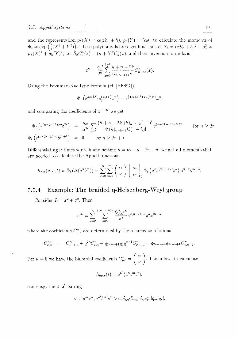
7.5. Appel! systems 101
and the representation Ph (X) = 0:( xOx + h), Ph (Y) = i0:6x to calculate the moments of
<Pt = exp (HX 2 + y 2 )). These polynomials are eigenfunctions of Sh = (xox + h)2 - 6; = Ph(X)2 + Ph(y)2, i.e. She~(X) = (n + h)2e~(x), and their inversion formula is
1 [5-] h + 2k xn = qn' "Ç""' n - Ch (x).
')n L..i (h) k' n-2k - k=O. n-k+l ;
Using the Feynman-Kac type formula (cf. [FFS97])
and comparing the coefficients of x n - 2r we get
ru. (p(n-2r+h)aab2r+ 1Î ~, \ ~ J o for n 2 21' + 1.
for ri 2 :21',
Differentiating 1/ times W.r.t. h and setting h = m -11 + 21' - n, we get all moments that are needed to calculate the Appell functions
7.5.4 Example: The braided q-Heisenberg-Weyl group
Consider L = x 2 + Z2. Then
n 2(n-v)1\2v en tn tL "Ç""' "Ç""' v, 1<- 2(n-v)-rc 1<- 2v-I<-e = L..i L..i --z . Y x
nl v=O
where the coefficients el~rc are determined by the recurrence relations
For K, = 0 we have the binomial coefficients e~o = ( : ). This allows to calculate
using e.g. the dual pairing

102 Chapitre 7. Evolution Equations and Lévy Processes on Quantum Groups
7.6 Densities
For one single variable, or in the commutative case, one can use Bochner's theorem to associate a density to a quantum random variable, cf. [Mey93].
We now want to associate joint densities to several non-commutating variables, along the li ne of Wigner distributions [Wig32]. We will map functionals on an algebra with n generators to me as ures on lRn. Equivalently, we can ask for a map from functions on lRn ( e.g., polynomials) to elements of the algebra.
Consider the following diagram:
Wigner QS ---t CS
Duality t t Duality QO ~ CO
Weyl
where QS: (linear span of) the set of quantum states CS: (linear span of) set of classical states
QO: set of quantum observables CO: set of classical observables
We want the following similar diagram:
"Wigner" U ---t M(X)
q-Fourier t t Fourier A ~ C(X)
"Weyl"
where X is the undeformed space or group, and M(X) denotes the (convolution) algebra of (signed) measures on X, C(X) the algebra of continuous functions on X, and A and U the quantum group and algebra. The q-Fourier transformation (with respect to an integral J) is defined by
F(u) = !(uexp)
where exp is the exponential or coevalution map, see also [KM94, Koo95]. We also have f(ab) =< F(a),b >. and thus in this setting a density (w.r.t. fA) of a functional ~ E A* can, at least in principle, be calculated with the inverse Fourier transform, Pib = FAI (~). A more detailed discussion, including an explicite example on lRq , can be found in [FS96b].
Here we shall use the right-hand-side of the diagram to introduce densities that 'live' on the classical, i.e. undeformed, group or space. Following Anderson[And69], we fix a set of generators Xl, ... ,Xn of A and define the Weyl map [Wey31] on polynomials U~l ... u~n by

7.6. Densities 10:3
where k = kl + ... + kn . Other definitions are possible, e.g. T-Vw : U~l •.. u~n 1----7 X~l ... x~n ("Wick"), or WAW : U~l ••• u~n 1----7 x~n ... X~l ("Anti-vVick"), or also T-Vq- exp defined by eU ' v 1----7 exp(xlv). But Wq- exp will not leave the marginal distributions unchanged. In fact,
W is uniquely determined by the conditions W(Ui) = Xi and W ((alui + '" + an'Un)k) = (al vV( ud + ... +an W( un))k, and thus only W* will give the correct marginal distributions for alllinear combinat ions of the generators. Ordered monomials like the "\Nick" or "AntiWick" map still le ad to the right marginal distributions for the generators.
The Wigner map W* is defined by the condition
< <l>, VV( u) >= f udT-V*( <l»,
i.e. as the dual of the Weyl map. VV*(<l» is called the Wigner density of <l>. The Fourier transform of the measure W* ( <l» is
gq,(v) F(T-V*(<l»)(v) = f eiu'vdT-V*(<l»
< <l>, lV(eiu .v ) >,
where we assumed that we can interchange the limits involved, and that this series defines an analytic function.
If the functionals <l>t form a convolution semigroup, then the associated \Vigner densities satisfy an evolution equation or Fokker-Planck-type equation.
Proposition 7.6.1 Let {<l>t; t E IR+} be a convolution semigroup with generator L, Le.
~~ <l>t = L<l>t = <l>tL. Suppose further that lV isinvertible. Then the Wigner distribution of <l>t satisfies
:t W*( <l>d = p(L )*W*( <l>t)
with p(X) = lV- 1 0 p(X) 0 W and p(X)* defined by duality.
Pro of: Differentiate < <l>t, T-V(u) >= f udlV*(<l>t)
with respect to t, on the right hand si de we get J ud dW~~q,,), while the left hand side gives
< L<l>t, lV(u) >=< <l>t,p(L)lV(u) >=< <l>t, T-V(p(L)u) >
f p(L )udlV*( <l>t) = f ud (p(L )*W*( <l>t)) .
7.6.1 Example: The braided Hne
Here we have only one variable, and the algebra is commutative, so the Weyl map is just ltV :un 1----7 xn. The Fourier transform of the functional <l> = E~=o anpn is thus
co '(' )n () i!i. iux "'"' anqn;LU gq, u =< '±', e >= L-. n! n=O

104 Chapitre 7. Evolution Equations and Lévy Processes on Quantum Groups
where we assumed that the regularity conditions necessary for interchanging the limits are satisfied. E.g. for ~a = eap , i.e. the functional determined by ~a(e:lp) = eap (where ex1p = "'00,- Xnpn) we get
q L..m_O qn!
( ) _ ~ qn!(iau)n g;Pa u - L..t (1)2
n=O n.
We need p(p)* to be able to give the form of the Fokker-Planck equation. Because of the simple form of W we have p(p) = O. The adjoint of the q-difference operator is a multiple of the q-difference with q replaced by q-I,
so that the Wigner density 'f/t( dx) = dW*( <I>t) of the semigroup with generator L = L cnpn satisfies
'7 a. 2 I.U. Example: The braided plane
[ n+m 1 ( ) ~ n q 'n+m i!i. n m n m
g;p VI, V2 = L..t ( )' Z < 'l:', X Y > VI V 2 • n,m=O n + m .
For the Gauss functionals in the sense of Bernstein (<I>(xnym) = znom,o or zmon,o, see [FNS96]) we get g;p(v) = eiZVl or g;p(v) = é ZV2 , i.e. W*(<I» is a Dirac mass in (z,O) or (0, z).
To write down the Fokker-Planck equations for Wigner distributions we need the representation p. For the two generators we get
7.6.3 Example: The q-affine group "lU t W n m ",n n!m! An+mf3n-v Vbm h th AN dt' d b vve ge : U I U 2 r-t L..,v=O (n+m)! n,va, W ere e nv are e ermlne y
A;;v = ° if n > N or v > n or n < 0, A~ = 1, A~v = ONv, and

7. 1. Conclusion 10.)
For the special case where the two lower indices are identical, we get A;;n = ( 1: ). The
Weyl map and its inverse are characterized by
W
vV- 1
This allows to write down p and thus the Fokker-Planck equation for any Lévy process. For X we simply get p(X} = 8~1 ' the expression for p(Y) is more complicated.
7.6.4 Example: The q-Heisenberg-Weyl algebra
The q-Heisenberg-vVeyl algebra HvVq can be treated in the same way. Choose a, b, cas
generators of HW then the Weyl map is given bv VV : unu:r'u r t---7 ",n~r n!m!r!D~;nmk+r an-kbm+kcr-k ql • 1 2 3 L.,k_O (n+m+r)'
where the coefficients D~~;+r are defined by
nN .L../n,r,k o if Tl < 0 or T < 0 or n + T > N or k < 0 or k > n /\ T,
DN ( AnT ) , n,O,O if 0 < n < N
DN - (j~), O,r,O - , if 0 ::; T ::; N
and the recurrence relation
D N + 1 _ D N + DN + k-m DN + ( -1) n,r,k - n,r,k n,r-1,k q n-1,r,k q r-k+1 ( 1) N 1- - Dn_1 rk-1'
q "
7.7 Conclusion
We gave a relation between stochastic processes and evolution equations on quantum / braided groups, and illustrated it on sever al examples. Two types of evolution equation were considered. First, we let the generator of the process act via the dual representation on the quantum or braided group itself. Solutions to these evolution equations are given in terms of Appell systems. vVe showed on several examples how they can be calculated. To get the second kind of evolution equation we associated \-Vigner-type distributions to the processes and functionals. These distributions are distributions on the undeformed space, and we thus get evolution equations for ordinary functions. If we replace the Weyl map by other maps, e.g. those corresponding to normal ordering ("Wick" or "Anti-\-Vick") or to q-exponentials, then we can hope to get simpler expression for p and thus for the Fokker-Planck equation, but the relation between the moments of the functionals and their "Wigner" distributions becomes more complicated.

106 Chapitre 7. Evolution Equations and Lévy Processes on Quantum Groups

Chapitre 8
Brownian Motion on -the Affine Group and Generalized Gegenbauer
Polynomials
Philip Feinsilver 10 Uwe Franz
\Nork in Progress
Résumé
Polynomial eigenfunctions of the generator of Brownian motion on the affine group are studied in a representation using a general shift operator. This yields a generalization of Gegenbauer polynomials. We determine the matrix elements of the group element and a variant, derive addition formulae, and give the conditions these polynomials to form a family of orthogonal polynomials.
10. Dept. of Mathematics, Southern Illinois University at Carbondale, IL 62901, USA, Email: [email protected]
107

108 Chapitre 8. Brownian Motion and Generalized Gegenbauer Polynomials

8.1. Introduction 109
8.1 Introduction
Let 6,6, ... , f;,d denote a basis for a Lie algebra of finite dimension d. Using McKean's product integral ([McK69], see also [FFS97]) to construct Brownian motion on the corresponding Lie group leads to the generator is 5 = f;,i + f;,~ + ... + f;,J. Here we study the two-dimensional non-abelian Lie algebra corresponding to the affine group acting on the realline. We may take as basis 6 = X,6 = L acting on x n with 6 = xD + a, i.e., 6 xn = (n + a) xn, for some constant a, and L is a general form of lowering operator acting as Lxn = bnxn- 1 ,with bo = 0 and bn =1 0 for n 2: 1. Defining ln = b1b2 · .. bn for n 2: 1, with 10 = 1, on the basis X n = xnlln we have f;,lXn = (n + a)Xn and LXn = X n - 11
n 2: 1, LXo = 0 We will find polynomial eigenfunctions of the generator S. For L = cl:' these are the
Gegenbauer polynomials. We thus dub our polynomials generalized Gegenbauer polynomials. Matrix elements for the affine group and variants, in this polynomial basis are found. Then we consider conditions for these to be a family of orthogonal polynomials. Some remarks about Appell sequences conclude the study.
8.2 Brownian motion on the affine group
Let G be the two-dimensional Lie Group G = {(a, b); a E IR+, b E IR} with multiplication (a,b) 0 (a',b') = (aa',ba' + b'), this is the group of affine transformations on the real line, (a, b) : x I-t ax + b. Let 11 be the associated Lie algebra, i.e. 11 has basis {X, L} with commutation relations [L, Xl = L. If we require X to be diagonal and suppose that there is a countable basis {en} that can be labelled by its X-eigenvalues Àn' then [L, p]en = L(Pm - Pn)Lnmem = L Lnmem = Len shows that L can only map the basis element with eigenvalue Àn to one with eigenvalue Àn - 1. Excluding the case that the representation space is the direct sum of sever al invariant subspaces we thus get X en = (a + n )en and Len = bnen for some constant a and some sequence {bn; n E IN}, bo = 0, bn E Œ x = Œ 1 {O} for n 2: 1. L is a generalized shift operator, such operators have been studied in umbrai calcuIus, cf. [BL96]. We will assume en = xn, then we can write -VT D d L "'00 1 k-1D k h l ",n (-l)n-k b "'\. = X + a an = L..-k=l k X , W ere n = L..-k=l k!(n-k)! k·
\iVe define a generalized factorial/o = 1, ln = b1b2 ..• bn , and a generalized exponential series e( x) = Ln=o ~: ' it is an eigenfunction of L.
vVe use McKean's product integral ([McK69], see also [FFS97]) to construct Brownian motion on the affine group. Its generator is 5 = X 2 - L2 .
If we look for polynomials eigenfunctions of S,
n
SPn(x) = ÀnPn(x), where Pn(x) = I:pnvx v, v=o
we find by comparing the coefficients of xn that the eigenvalue has to be Àn = (n + a)2. Comparing the coefficients of xn-l we see Pn,n-l = O. Looking at XV we get the recurrence relation

110 Chapitre 8. Brownian Motion and Generalized Gegenbauer Polynomials
Solving this recurrence we find that the polynomial eigenfunctions of Sare generalized Gegenbauer polynomials,
"-Of ( ) = '" ~ (a )n-k ( -1 )k n-2k 'fin X L..... () kk' X , In-2k a n 4 .
or, in a different normalization,
The second normalization has the advantage that we get the usual Gegenbauer polynomials C;: (x) in the conventional normalization as special case bn = n; the cjJ~ are determined by the condition that the highest coefficient is equal to one, this form can also be used for a = o. We will from now on assume a > -1.
Proposition 8.2.1 We have the inversion formulas
[.!.!.] ~ ~ (a)n-2k+1_1_cjJOf (~) t:o In-2k (a )n-k+l 4k k! n-2k\.L
ln [~] a + n - 2k - Of - 2n L () k' Cn_2k (X).
k=O a n-k+l .
Proof:
[.!.!.] ~ ~ (a)n-2k+1 1 "-Of () L..... ( ) 4kk' 'fIn-2k X k=O In-2k a n-k+l .
[~] ( ) [~]-k ( ) ()l L ~ a n-2k+1 1 L In-2k a n-2k-l -1 n-2k-21 k=O In-2k (a)n-k+1 4kk! 1=0 In-2k-21 (a)n-2k 41[! x
ï: ~ xn- 2m f (_l)m- JL (a + n - 2/-l)(a)n-m-JL
m=O In-2m 4m JL=O /-l!(m -/-l)! (a)n-JL+l
[~] ln xn- 2m m (m) (-1)JL(a+n-2m+2/-l)
fo In-2m 4mm! ~ /-l (a + n - 2m + /-l) ... (a + n - m + /-l)
=: 'Em(a + n - 2m)
if we substitute /-l t-+ m - /-l. For m = 0 we get xn, i.e. the desired result. We will now show by induction that 'Em(a + n - 2m) gives zero for m ~ 1 and a arbitrary. For m = 1 we have
,8 + 2 = O. (,8 + 1 )(,8 + 2)
Assume now that 'Em(,8) = 0 for aIl ,8, then we get
1 o = ,8 + m + 1 ('Em(,8) - 'Em(,8 + 2))

8.3. Group elements and matrix elements 111
p+m+l
m+l { ( ; ) (p + m + 1 + /1) + ( /1 : 1 ) (p + /1) } ( -1 )'"(p + 2/1)
]; (p + m + 1) (p + /1) ... (p + m + 1 + /1)
~m+l (p),
since ( ; ) (p + m + 1 + /1) + ( /1: 1 ) (p + I-l) = ( m: 1 ) (p + m + 1). The inversion
formula for the è~ (x) follows immediately. 1
8.3 Group elements and matrix elements
USiIlg coordinates of the second kind vie cau v/rite a group element of the affine grou_p
as g(A, B) = eAX eBL ,
in these coordinates the group law has the form
g(A., B)g(A', B') = g(A + A', BeA' + B').
It is also interesting to consider the 'group-like' element defined by
§(A, B) = eAxe(BL),
in the following section we will investigate for which cases their is sorne kind of group law or multiplication rule for §(A, B).
We define the matrix elements of g(A, B) and §(A, B) W.Lt. to the è~ by
g(A, B)C~(x)
§(A, B)C~(x)
L Mmn(A, B)è~(x),
L i1mn(A, B)è~(x).
Proposition 8.3.1 The matrix elements are
for 0 ::::; p ::::; n, and where a = eA and the summation index /1 takes the values P, p - 2, p -4, ... ,0 or 1 according to whether p is even or odd.

112 Chapitre 8. Brownian Motion and Generalized Gegenbauer Polynomials
where we recognize the (generalized) Gegenbauer polynomials insides the brackets for the matrix elements of g(A, B) (or g(A, B), respectively). •
Remark: The fact that the matrix elements of g( A, B) contain the usual Gegenbauer polynomials and not the generalized ones follows from the relation L = U- 1 DU, where U is defined by U xn = ~, D = cl:' if we note eAX eBD = U g(A, B)U-1, and C~(x) = Ue~(x).
8.4 Multiplication rules and addition formulae
The group law of the affine group leads immediately to an addition formula for the associated matrix elements,
n
Mpn(aa' , Ba' + B') = L L Mrn(a, B)Mpr(a' , B'). r=O r
Proposition 8.4.1 We have
C~~:(Ba' + B') = t L C~~:(B)C:!":;' (B') (a + r)((a')JL'-JL r=O JL' (a + p') I-":;r H (JL~r)!
Proof: Applying g(aa' , Ba' + b') = g(a, B) 0 g(a', B') to e~(x) and using Proposition 8.3.1 we get
~ '" Ca+JL(B ' + B') (a + p) (aa')JL ea( ) = L...L... n-JL a (+) _ (JL-P), P x p=O JL a p TH 2 •
~"'ca+JL'(B') (a+r) (a')JL' ~"'ca+JL(B) (a+p) aJL ea(x). L...L... n-JL' ( ') (fL'-r), L...L... r-JL ( ) (/1::2.)' p r=O JL' a + p I-":;r H 2 • p=O JL a + p TH 2 .
Comparing the coefficients of aJLe; (x) yields the proposition. •
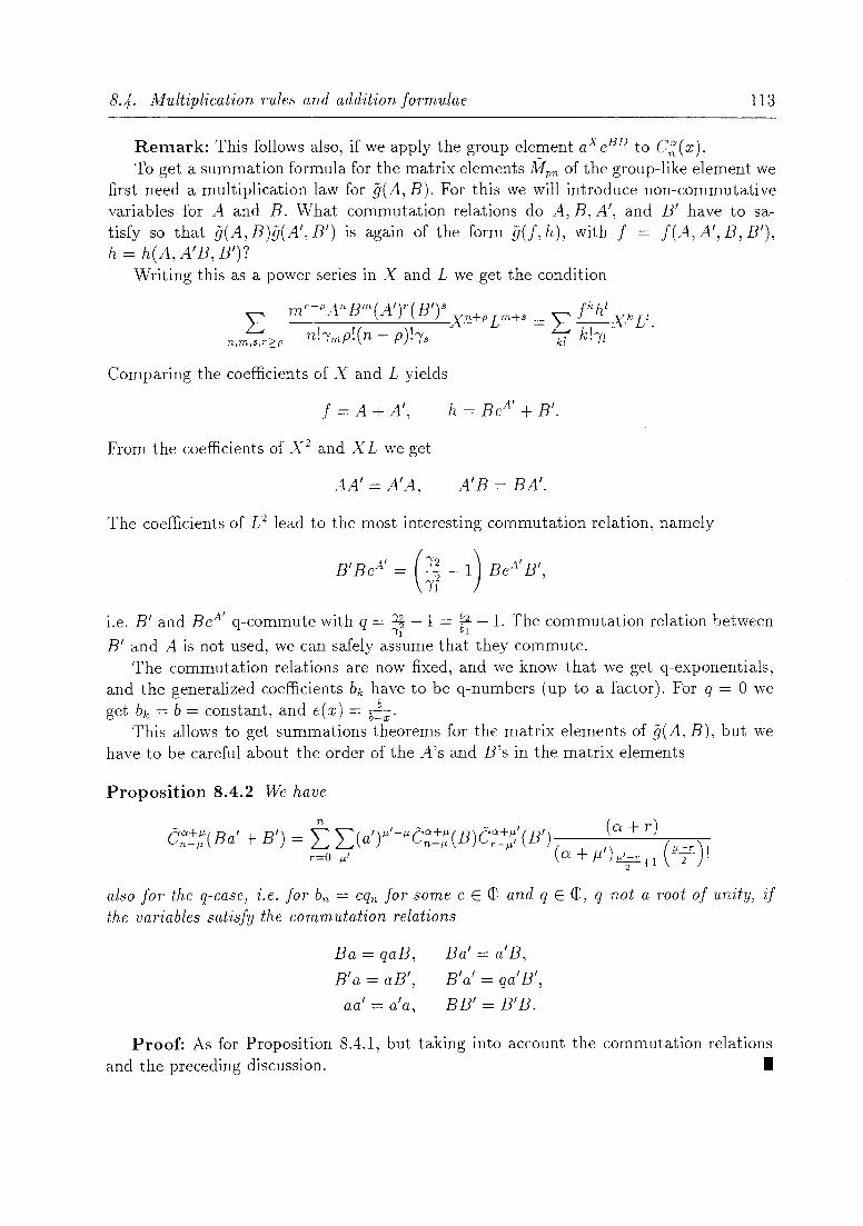
8.4. Multiplication rules and addition formulae 113
Remark: This follows also, if we apply the group element aXeBD to C;:(x). To get a summation formula for the matrix elements iVIpn of the group-like element we
first need a multiplication law for g(A, B). For this we will introduce non-commutative variables for A and B. What commutation relations do A, B, A', and B' have to satisfy so that g(A, B)g(A', B') is again of the form g(J,h), with f = f(A,A',B,B'), h = h(A, A' B, B')?
vVriting this as a power series in X and L we get the condition
n,m,s,r2:p
Comparing the coefficients of X and L yields
f = A+A', h = BeA' + B'.
From the coefficients of X 2 and XL we get
AA' = A'A, AIB = BA'.
The coefficients of U lead to the most interesting commutation relation, namely
B' BeA' = (12 - 1) BeA' B' 2 ' Il
i.e. B' and BeA' q-commute with q = ~? - 1 = ~ - 1. The commutation relation between
B' and A is not used, we can safely assume that they commute. The commutation relations are now fixed, and we know that we get q-exponentials,
and the generalized coefficients bk have to be q-numbers (up to a factor). For q = 0 we get bk = b = constant, and e( x) = b~x'
This allows to get summations theorems for the matrix elements of g(A, B), but we have to be careful about the order of the A's and B's in the matrix elements
Proposition 8.4.2 We have
also for the q-case, i.e. for bn = cqn for some c E <C and q E <C, q not a root of unit y, if the variables satisfy the commutation relations
Ba = qaB,
B'a = aB', , ,
aa = a a,
Ba' = a'B,
B'a' = qa'B',
BB' = B'B.
Proof: As for Proposition 8.4.1, but taking into account the commutation relations and the preceding discussion. 1
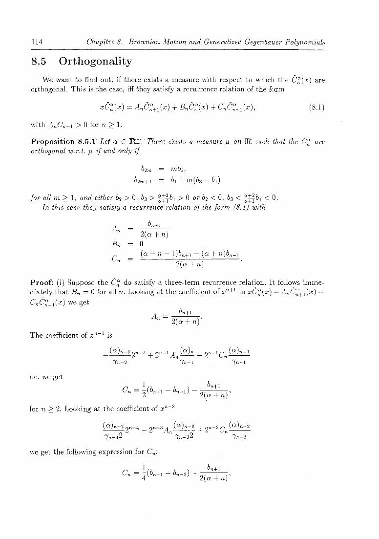
114 Chapitre 8. Brownian Motion and Generalized Gegenbauer Polynomials
8.5 Orthogonality
We want to find out, if there exists a measure with respect to which the è;:;(x) are orthogonal. This is the case, Hf they satisfy a recurrence relation of the form
(8.1 )
Proposition 8.5.1 Let 0: E IIt.+-. There eXists a measure 11 on IR such that the C;:; are orthogonal w. r. t. 11 if and only if
mb2 ,
bl + m(b3 - bd
for aIl m ~ 1) and either b2 > 0) b3 > ~t~bl > 0 or b2 < 0, b3 < ~t~bl < O. In this case they satisfy a recurrence relation of the form (8.1) with
L Un+l 2(0: +n) o (0: + n - l)bn+1 - (0: + n)bn - l
2(0:+n)
Proof: (i) Suppose the è;:; do satisfy a three-term recurrence relation. It follows immediately that En = 0 for an n. Looking at the coefficient of xn+l in xè;:; (x) - An è;:;+l (x) -
Cnè;:;_l(X) we get
The coefficient of xn-l is
_ (0:)n- 1 2n- 2 + 2n - 1 An (O:)n _ 2n-ICn (O:)n-l in-2 in-l in-l
i.e. we get 1 bn+1
Cn = 2"(bn+1 - bn-d - 2(0: + n)'
for n ~ 2. Looking at the coefficient of xn-3
(0:)n-22n-4 -2n-3An (0:)n-3 +2n- 3Cn (0:)n-2 in-42 in-32 in-3
we get the following expression for Cn:

8.5. Orthogonality 115
for n 2: 4. Equating those two expressions we find
for n 2: 4. For n = 0,1,2 the recurrence is satisfied with Ao = .g;, Al = 2(~~1)' Cl = 2(~~1)'
A -~ C -h±._~ 2 - 2(cx+2) ' 2 - 2 2(cx+2)'
For n = 3 (and a =1- 0) we find that the recurrence is only satisfied if b4 = 2b2 , and th t<· th' A - ~ - JlL d C - cx+2 b a III lS case 3 - 2(a+3}. - cx+3- an 3 - a+3 2·
Checking Al C2 > 0 we see that either b2 > 0 and b3 > :!î b1 or b2 < 0 and b3 < ~!î bl ·
AoCl = 2t~~1) > 0 implies that b1 and b2 have the same sign, A2C3 = 2t~~'3) implies that b2 and b3 have the same sign. .
(ii) We will now show that these are the only restrictions on the bn necessary in order to get a three term recurrence relation. Let bl , b2 , b3 be arbitrary, and set (bo = 0)
Then with
we get (for n 2: 4)
bn+1
2(O'+n)
bl + m(ba - bd, mb2 •
b2 _ 4 _ O'+m b 2 . 2m+l - 2(0' + 2m + 1) 2
b3 - bl _ A _ (a + m) (b3 - bl ) - bl
2 2m - 2(0' + 2m) ,
Anè~+l (x) + Cnè~_l (x) [!W.]
An t (O')n+l-k( _,I)k (2xt+l- 2k k=O /n+l-2k k .
[n;l] k
+Cn L (O')n-l-k(-,I) (2 xt- 1- 2k k=ü /n-1-2k k .
4 (a )n+l (,> )n+l ., n ~x
/n+l
[!W.] + t (O')n_k(-I)k(2x)n-2k x (An 2(O'+n-k)-Cn2k)
k=l /n-2k k! bn+1- 2k
xè~(x)
since An2( 0'+ n - k) - Cn2k = bn+l - k(bn+1 - bn-d = bn+l-2k ' If in addition b2 > 0 and b3 > ~!~ bl > 0 or b2 < 0 and b3 < :!~ b1 < 0 then one can
check that An Cn+1 > 0 for all n. E.g. on the odd numbers, n = 2m + 1, we find that

116 Chapitre 8. Brownian Motion and Genemlized Gegenbauer Polynomials
b3 - ~!:!~ bl has to have the same sign as b2 for aIl m. 1
Proposition 8.5.2 The measure of orthogonality is
2r( 0' + 1) 2(3-1 2 a-(3
laf(0'-jJ+1)r(jJ)lx l (f-x) R[_-Y,-Yl(x)dx
Remark: The conditions. on bl; bz, bs areequivalent tOI> o and 0<: jJ < 0' + 1 For the special case bn = n (i.e. 1 = 1 ,i3 = ~, and therefore 0' > - ~) this reduces to the measure of orthogonality of the Gegenbauer polynomials
f(O'+l) 2(>_1
fl(dx) = 4a- 1/ 2J7iT(0' + D (1 - x) 2 R[-l,lJ(x)dx.
Proof: Using the inversion formula (Proposition 8.2.1) and orthogonality we get
J j' in [~l 0' + n - 2k a xndfl(X) = 2'11, ~ k!{O'L_L.-'-l Cn _ 2k (X)dfl
k=U \ -"" -n .. r.L
Rewriting 12m as
we get
if n even, n = 2m,
if n odd.
-(t) - J itxd (. ) - D ( b3~bl 1_ b2 (63 - b1 ) t 2 ) fl - e fl x - IrZ ~,O' + 1 16 .
for the Fourier transform of fl. Now we can use e.g. [Obe90, 1.2.23] to conclude. 1
8.6 Appell Systems
Definition 8.6.1 We cal! a family of polynomials {Pn; n E IN} a L-{bn}-Appell system, if
(i) Pn is a polynomial of degree n,
(ii) Lpn = bnPn-l'
Remark: The sequence {bn} can be replaced by any other sequence {bn }, if the Pn are rescaled accordingly:
is a L-{bn}-Appell system if {Pn} is a L-{bn}-Appell system.
Proposition 8.6.2 {rP~-n; n E IN} is a L-{bn}-Appell system.

8.6. Appel! Systems 117
An L-{bn}-Appell system Îs completely determined by the sequence {Pn = Pn(O); n E lN}, just like usuai Appell systems (see e.g. [FS92]). \Ve define a generating function
00 tn F ( x, t) = I: Pn ( X ) -.
n=O ln
This function satisfies LF(x, t) = tF(x, t), i.e. it is of the form
F(x, t) = e(tx)G(t)
where e(tx) is the generalized exponential series, e(tx) = L~=o (t~~n, and G(t) = F(O, t) = "'00 t n
L....n=o Pn'Yn'
Proposition 8.6.3 The L-{bn}-Appell polynomials have the form
Proof: Apply L 1/ times to Pn(x) = L~=oPnmxm and set x equal to zero.
For the Appell system {<p~-n( x)} we have
A.,cx-n() {O pn = 'f'n 0 = 1 if n is odd, if n is even, n = 2m.
4mm!( -cx+l)m
Rewriting the equation from Proposition 8.6.3 as
n () n-l v X _ Pn X ~ Pn-v X - - --- L..---' ln ln V=O In-v IV
and using it recursively to replace the powers of x, we get an inversion formula for L{bn}-Appell polynomials.
Proposition 8.6.4

118 Chapitre 8. Brownian Motion and Generalized Gegenbauer Polynomials
Chapitre 9
Limit Theorems on Quantum Groups
This chapter describes work in progress. The problems
are for~l~lated, approac~es are suggested, conjectur:s 1
or parlla] answers are gl ven, but the results are still incomplete.
Résumé
We examine the possibilities of giving limit theorems on bialgebras, including precise characterisations of the limit laws. First, we examine what can be obtained from results due to Schürmann [Sch93] and D. Neuenschwander and R. Schott (cf. [NS96]) in particular cases, focussing on explicit characterisations of the limit distributions.
Then we look for law of iterated logarithm type results. We formulate the problem, suggest a definition replacing that of the path-wise supremum in the classical law of iterated logarithm for quantum stochastic processes, and propose an approach for calculating the law of this supremum.
In Section 9.4, we study a different kind of limit theorem, combining classical random variables and quantum random variables. Here the convolution of the functionals is chosen according to a sequence of classical Li.d. random variables.
119

120 Chapitre 9. Limit Theorems on Quantum Groups

9.1. Introduction 121
9.1 Introduction
We want to get limit theorems on bialgebras, and as explicit as possible. The limit theorems by M. Schürmann [Sch93, Theorem 6.1.1,6.1.2, and 6.1.3] apply in a very general context, using only the coalgebra structure, but do not give mu ch information about the explicit form of the limit distributions.
Feinsilver [Fei87] and Neuenschwander and Schott [NS96] follow a different approach. On the braided line the q-convolution can be defined for usual (signed) measures on the real line, an.dthus we are not restricted to moment methods. This convolution does not conserve positivity, so in general the limit distributions are not positive. Also, even though [Fei87, Theorem 3] states that the q-characteristic function 1j;( t) = f e~txdf.l( x) characterizes uniquely the measure f.l, we do not know how to explicitely calculate f.l from 1jJ.
In the first part (Section 9.2) we will look for analogues of the law of large numbers, centrallimit theorem, etc. Here our results mostly follow from previous work, in particular M. Schürmann[Sch93], Ph. Feinsilver[Fei87], and D. Neuenschwander and R. Schott[NS96].
In the second part (Section 9.3) we attack the question of the existence of limit theorems of the form of the lavv of the iterated logarithm.
The study of analogues of trajectorial properties (as e.g. the la\'\' of the i terated 10-garithm) of quantum processes is related to the question of the existence of classical versions, see e.g. [BKS96]. Thus the definition of the supremum of quantum random variables should coincide vvith the corresponding supremum of their classical versions, if these exist. Since the quantum pro cess only determines the finite joint distributions of the classical process, vve also have to address the question which classical version (left or right continuous, càdlàg, etc., if they exist) should be taken.
In the next section vve prove a limit theorem that combines classical random variables and quantum random variables. The limit theorem in this section is motivated by R. Speicher's article[Spe92].
In Section 9.5, vve replace the scaling in the normalization by more general operators.
9.2 Analogues of the law of large numbers and the central limit theorem
9.2.1 General results for limit theorems on bialgebras
The most general result is probably the follovving theorem due to M. Schürmann.
Theorem 9.2.1 ([Sch93, Theorem 6.1.1] Let ynk, n E lN, k = 1, ... , kn (kn E lN), be tinear functionals on a coalgebni C satisfying
(i) Ynl, ... , ynkn commute for each n E lN with respect to convolution,
(ii) limn-too liml<k<kn I(ynk - c)(c)1 = 0 for aU c E C,
(iii) sUPnElN L19~kn I(ynk - E)(c)1 < 00 for aU c E C.

122 Chapitre 9. Limit Theorems on Quantum Groups
Furthermore, suppose that there is a linear functional 'IjJ on C such that for al! c E C
Then
J1~ (. il <pnk) (c) = (exp* 'IjJ)(c) 1~k9n
for al! c E C (wher:e the praduct.I1*. is .. the.. convolution.p.r.oduct.).
We will use a corollary of this theorem for lN-graded coa1gebras. Let C be an lN-graded coa1gebra, i.e. C = EBnElN c(n) and ~c(n) ç EBnl +nz=n c(nJ) 0 c(nz ). Then we can define a sca1ing s : Œ x C -+ C by setting
s(z)c = z-deg(c)c,
for c E C(deg(c)), and extending linearly in the second argument. With this definition we have (<p * 'IjJ) os(z) = (<pos(z))*('ljJos(z)) for alllinear functiona1s cp, 'IjJ on C and aIl z E Œ.
Corollary 9.2.2 ([Sch93, Theorem 6.1.3]) Let C be an lN-graded coalgebra and let fi, E IN. If a linear functional <p on C satisfies
(i) <PIC(l) = 0 for 0 < 1 < fi"
(ii) <PIc<O) = elc<O) ,
then for al! c E C
where g<p' denotes the linear functional on C with
g<pIC(l) 0 for alll =1= fi"
g<plc(l<) = <pIC(").
9.2.2 The braided line
The study of the 'q-convolution' and related 1imit theorems was initiated by Ph. Feinsi1ver [Fei87]. In this case the convolution can be defined via a q-characteristic function, and it is therefore possible to consider also measures that are not characterized by their moments. Thus we can look e.g. for analogues of stable laws (cf. [NS96]).
Application of Corollary,9.2.2 gives the following result
Proposition 9.2.3 Let fi, E lN, <p: lRq -+ Πnormed, and <p(x) = "'<p(X"-l) = O. Set <pn = <p*n 0 s(n1/"), then
where c = <p(x")jq,,!
1· cpl< lm <pn = e ,
n-too
For !ql < 1, Neuenschwander and Schott's result [NS96] allows to extend the previous proposition to fi, E]O,2[, if ecpl< is interpreted as the q-characteristic function of the limit distribution.

9.3. Law of iterated logarithm type results 123
9.2.3 The braided q-Heisenberg-Weyl group
We take the grading that assigns degree one to the two primitive generators. Then, with Corollary 9.2.2, we find exactly the functionals that belong to Gaussian convolution semigroups in the sense of Subsection 6.6.1 (cf. Proposition 6.6.8) as Emit distributions of the law of large numbers and the central limit theorem (i.e. for K, = 1, and K, = 2, respectively) .
9.3 Law of iterated-logarithm ·typeresults
Let (Bt )tEJR+ be standard Brownian motion on IR. We have the following classical descriptions of the asymptotic behavior of Bt.
Theorem 9.3.1
Theorem 9.3.2
1. Bt Imsup -----r::;::::::;::=ë=== Hoo y'2t log log t
1 p.s.
.. . ~ Bt llm m! -----r::;::::::;::=ë===
Hoo y'2t log log t -1 p.s.
1 . . JlOg log t il hm mf sup .IBsl = JO
t-+oo t 1 ~s~t V 8 p.s.
Is it possible to state and prove similar results for quantum stochastic processes? For classical processes the supremum sup sE[O.t] X s is taken for a fixed element w of the
underlying probability space D, i.e. for each w E D we take the supremum of the trajectory yw = X,,(w) : s f-t Xs(w).
Our first step will be to define an analogue of the supremum for quantum stochastic processes. In or der to be meaningful such a definition should le ad to the same distributions as the classical one, if the process has a classical version. This problem is treated in Subsection 9.3.l.
The final goal should be to construct sup sE[O,t] X s or lim SUPHoo Xt, lim infHoo X s as an operator, in the same operator algebra as (XS)SEI, e.g. acting on sorne Fock space. But for a first approach we satisfy ourselves with a construction of the law of sUPsE[O,t] X s .
In Subsection 9.3.2 we devise an approach for calculating the law of finite suprema of (quantum or classical) random variables using their characteristic function and the Hilbert transform.
9.3.1 Definition of the supremum for quantum stochastic variables
In this section quantum random variables will be self-adjoint operators (say bounded) on a Hilbert space, and quantum stochastic processes will be families of such operators. Thus IXt l, O!\ Xt, 0 V X t can be defined via spectral calculus, as well as X s V X t , as long as X s V X t commute. Let X = IJR '\dE). be the spectral resolution of X, and <I> = I: < Vi, 'Vi >
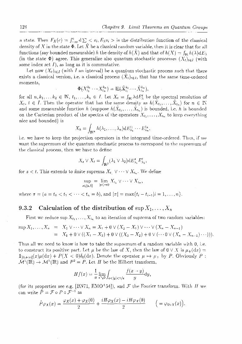
124 Chapitre 9. Limit Theorems on Quantum Groups
astate. Then Fx(c) = 1':00 dL < Vi, E>,Vi > is the distribution function of the classical density of X in the state q,. Let X be a classical random variable, then it is clear that for aIl functions (say bounded measurable) h the density of h(X) and that of h(X) = IlR h(>')dE>. (in the state q,) agree. This generalize also quantum stochastic pro cesses (Xt)tEI (with sorne index set I), as long as it is commutative.
Let now (Xt)tEI (with J an interval) be a quantum stochastic pro cess such that there exists a classical version, i.e. a classical pro cess (Xt)tEI, that has the same time-ordered moments,
for aIl n, kt, . . , k2 E lN, t l , ... , kn E J. Let Xt = IlR >'dEl be the spectral resolution of Xt, t E J. Then the operator that has the same density as h(XtI , ... , Xtn) for n E lN and sorne measurable function h (suppose h(XtI , . .. , Xtn) is bounded, i.e. h is bounded on the Cartesian product of the spectra of the operators X tI , ... ,Xtn to keep everything nice and bounded) is
i.e. we have to keep the projection operators in the integrand time-ordered. Thus, if we want the supremum of the quantum stochastic process to correspond to the supremum of the classical process, then we have to define
X s V Xt = [ (>'1 V >'2)dE~ El , lIB.? I 2
for s < t. This extends to finite suprema X tI V ... V Xtn' We define
sup = l~m X tI V ... V Xtn , sE[a,b] Ipzl--+O
where 7r = (a = to < t l < ... < tn = b), and 17r1 = max{ti - ti-di = 1, ... , n}.
9.3.2 Calculation of the distribution of sup Xl, ... ,Xn
First we reduce sup X tI , ... ,Xtn to an iteration of suprema of two random variables:
supXI , ... ,Xn - Xl V··· V X n = Xl + 0 V (X2 - Xd V··· V (Xn - Xn- l )
Xl + 0 V ((Xl - X 2) + 0 V ((X3 - X 2) + 0 V (···0 V (Xn - Xn-d" .))).
Thus all we need to know is how to take the supremum of a random variable with 0, i.e. to construct its positive part. Let p be the law of X, then the law of 0 V X is p+ (dx) = D.]O,+oo[(x)p(dx) + P(X < O)Jo(dx). Denote the operator p H- p+ by P. Obviously P : M I (1R) -+ M I (1R) and p2 = P. Let H be the Hilbert transform,
Hf(x) = ~ liml f(x - y) dy, 7r e').O e<lyl<l/e y
(for its properties see e.g. [BN71, EMO+54]), and F the Fourier transform. With H we can write P = F 0 P 0 F- I as
PA () _ <px(x) + <px(O) iH<px(x) - iH<px(O) <Px x - 2 + 2 ( = <pov x ( x ) ) .

9.3. Law of iterated logarithm type results 125
Passing from (Y, Xl, Xz) to (Y, Xl V Xz) can be decomposed into the following steps, an of which can be translated into operations on the joint characteristic function:
ep(Y,XI ,Ov(X2 -XI)) (u, VI, Vz) = FV2 ep(y,X1 ,X2 -Xd(U, Vl, vz)
where the subscript of P"2 indicates that it acts on the variable Vz. We thus get a new operator S = SVI,V2-+ V : y(y,X 1,X2 )( U, VI, vz) f-t y(Y,X I VX2 )( U, V),
Sy(y,X I ,X2 )(U,V) ep(Y,X) VX2 )( u, v) y(y,X I ,X2 )( U, V, 0) + ep(Y.XI ,X2 )( u, o. V)
where vP-J indicates that we have to take the Cauchy principal value of the integral at the singularities.
From its definition it is clear that S is 'associative', i.e. the or der does not matter if we iterate S, since (Xl V X 2 ) V X 3 = Xl V (Xz V X 3 ). This implies that there is a welldefined operator s(n), corresponding to n-fold suprema, and that sin) can be calculated by iterating S in any way we want.
Example: Processes with independent (and stationary) increments, If (Xt )tE1R+
is a process with independent and stationary increments, then the characteristic function of (Xtl , ~)[t2 - Xtl , ... ,Xtn - X tn _ l ) factorizes,
and the expression for the n-fold suprema simplifies considerably. vVe get
In the Emit n -+ 00, maXv=l, .. "n(tv - tv-d -+ 0 we should expect
( ) -- tÎ'oL(u)oÎ' 1 epsuPsE[O,tj X S U - e .
Note the reversaI of the time-order, i.e. Foe{tn-tn-dL(u) is the first to act on 1 = Pl. If the increments are independent, but not stationary, then the preceding discussion suggests
epSUPSE[O,tjXS(U) = G(O,t)l,
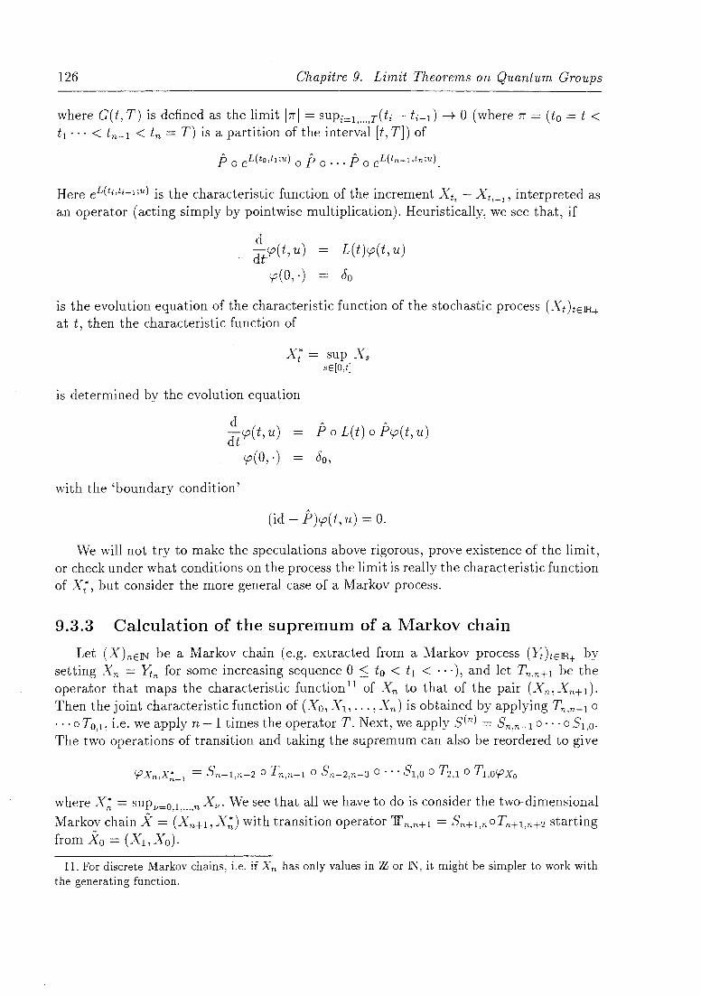
126 Chapitre 9. Limit Theorems on Quantum Groups
where G(t, T) is defined as the limit 171"1 = SUPi=l, ... ,T(t i - ti-d --70 (where 71" = (to = t < t l ... < tn-l < tn = T) is a partition of the interval [t, T]) of
Here é(i;,ti-l;U) is the characteristic function of the increment Xt; - X ti _ 1' interpreted as an operator (acting simply by pointwise multiplication). Heuristically, we see that, if
d -d cp(t.1 u)
t cp(O,·)
L(t)cp(t,u)
Jo
is the evolution equation of the characteristic function of the stochastic process (Xt)iElR+ at t, then the characteristic function of
x; = sup X s sE[o,il
lS determined by the evolutionequation
d dtCP(t,u)
cp(O, .)
with the 'boundary condition'
Po L(t) 0 Pcp(t, u)
(id - P)cp(t, u) = O.
We will not try to make the speculations above rigorous, prove existence of the limit, or check un der what conditions on the process the limit is really the characteristic function of Xt, but consider the more general case of a Markov process.
9.3.3 Calculation of the supremum of a Markov chain
Let (X)nElN be a Markov chain (e.g. extracted from a Markov process (Y~)tElR+ by setting X n = Ytn for sorne increasing sequence 0 ~ to < t l < "'), and let Tn,n+1 be the operator that maps the characteristic function 11 of X n to that of the pair (Xn, Xn+d. Then the joint characteristic function of (X01 Xl," . ,Xn) is obtained by applying Tn,n-l ° ... ° TÛ,l, i.e. we apply n -1 times the operator T. Next, we apply Sen) = Sn,n-l o· .. 0 51,0.
The two operations of transition and taking the supremum can also be reordered to give
COx x' = Sn-l n-2 0 Tn n-l 0 Sn-2 n-3 ° ... SI 0 0 T2 loTI o!OXo r n, n-l ' , , '" r
where X~ = sUPv=O,l, ... ,n Xv' Vve see that an we have to do is consider the two-dimensional
Markov chain X = (Xn+1,X~) with transition operator 1I'n,n+1 = Sn+l,noTn+1,n+2 starting from "X"o = (Xl, Xo).
11. For discrete Markov chains, i.e. if .ln has only values in 7l or lN, it might be simpler to work with the generating function.
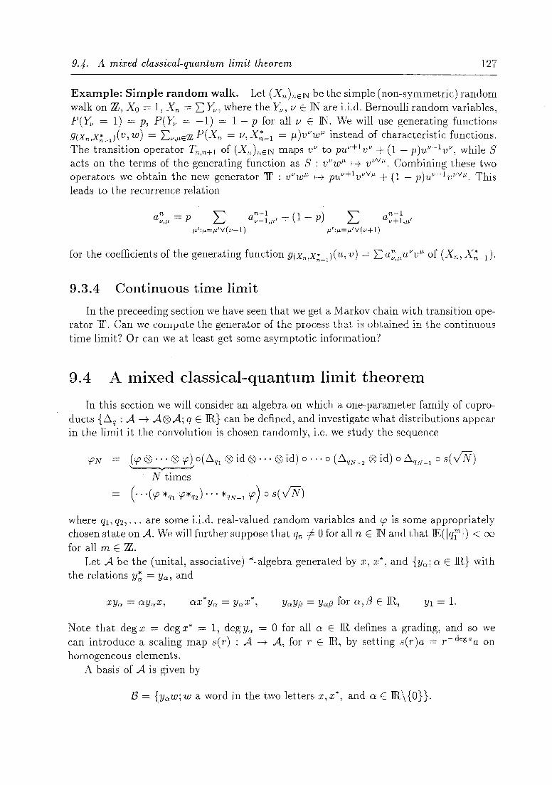
9.4. A mixed classical-quantum limit theorem 127
Example: Simple random walk. Let (Xn)nElN be the simple (non-symmetric) random walk on '!l, Xo = 1, X n = LYv , where the Yv , 1/ E IN are i.i.d. Bernoulli random variables, P(Yv = 1) = p, P(Yv = -1) = 1 - p for allI/ E IN. We will use generating functions g(Xn,X~_l)( V, w) = LV,iLE7l P(Xn = 1/, X~_l = 11 )VVwiL instead of characteristic functions. The transition operator Tn,n+1 of (Xn)nElN maps VV to puv+1v v + (1 - p)UV-1v v , while S acts on the terms of the generating function as S : VV wiL !---+ v Vv iL. Combining these two operators we obtain the new generator 11' : VVw iL !---+ pUV+IVVViL + (1 - p)UV-IVVViL. This leads to the recurrence relation
9.3.4 Continuous time limit
In the preceeding section we have seen that we get a Markov chain with transition operator 11. Can we cornpute the generator of the process that is obtained in the continuous time limit? Or can we at least get sorne asymptotic information?
9.4 A mixed classical-quantum limit theorem
In this section we will consider an algebra on which a one-parameter family of coproducts {6. q : A -7 A0A; q E IR} can be defined, and investigate what distributions appear in the limit it the convolution is chosen randomly, i.e. we study the sequence
if'lV = (if' 0··· 0 if') o(6.q1 0 id 0···0 id) o··· 0 (6.QN _ 2 0 id) 0 6.qN _ 1 0 s(VN) , v 1
N times
(- .. ( if' *ql if'*Q2) ... *qN-l if') 0 s( VN)
where ql, q2, . .. are sorne i.i.d. real-valued random variables and if' is sorne appropriately chosen state on A. We will further suppose that qn i- 0 for an n E IN and that IE( Iq~ 1) < 00
for aH m E 'Il. Let A be the (unital, associative) *-algebra generated by x, x"", and {Ya; a E IR} with
the relations Y~ = Ya, and
" " ax Ya = Ya X , YaY(3 = Ya6 for a, ,B E IR, YI = 1.
Note that deg x = deg x* = 1, deg Ya = 0 for aH a E IR defines a grading, and so we can introduce a scaling map s(r) : A -7 A, for r E IR, by setting s(r)a = r- dega a on homogeneous elements.
A basis of A is given by
B = {Yaw;w a word in the two letters x,x*, and a E IR\{O}}.

128 Chapitre 9. Limit Theorems on Quantum Groups
On this algebra we can define a whole family of coalgebras, depending on one parameter q E 1R, namely,
Ll.qx = x 01 + Yq 0 x,
and €q(x) = €q(x*) = 0, €q(Ya) = 1 for aIl a E 1R. In fact, for q =1= 0, the subalgebra Ao generated by {x, x*, Ya; a =1= O} is a Hopf algebra with the antipode Sq : Ao -+ Ao,
Using these different coalgebra structures we obtain different multiplications for functionais on A, i.e. a one-parameter family of convolutions,
for linear functionals 'P, '!jJ : A -+ <C. We state now the main result of this section (in a preliminary form).
Theorem 9.4.1 Let (qn)nElN be i.i.d. random variables with values in 1R\{O} such that lli(lqfl) < 00 for aIl m E 7l, and let 'P : A -+ <C be the state defined on the basis B by
"(Yo w) = { ~ ifw = 1, ifw = x*x, else.
Then the moments of 'P N = ( ... ('P *ql 'P) *q2 ... *qN -1 'P) 0 s( yiN) converge for N -+ 00 in probability to those of some functional 'Pcc.
Remark: We give the explicite form of 'Pcc in Corollary 9.4.2. Before we prove this theorem we will have to study the algebraic structure of the dual
of Ao.
9.4.1 The algebra U
Let x( w) be the functional defined by
x( w ) (ypw') = { ~ if w = w', else.
Then U = span {x( w); w E <C < x, x* >} is a subaigebra of the dual of Ao (with the multiplication mq = Ll.;). Let a E Ao, Ll.qa = L a~l) 0 a~2), then the product x( w) *q X( w')
is defined by (X(w). X(w'))(a) = Lx(w)(a~1))x(w')(a~2)). We get by induction

9.4. A mixed classical-quantum limit theorem 129
and from this we can also calculate the coproduct of any element of Ao. To calculate the product x( w) *q X( w') we have to see what elements of Ao have a term
YaW @ Yf3W' in their coproduct. Since the coproduct do es not change the total number of x's and x*'s, but just splits a ward into two, the product has to do the inverse. vVe get
X(w) *q X(w') = Lc~,w,(q)X(v), (9.1)
where v runs over an words that can be obtained by shuffiing w and w', and the C~,WI are polynomials in q andq-1. To get the explicite expression, use the following procedure.
In the first term v is simply the concatenation of w and w', and the coefficient is equal to one. Then move the letters of w ta the right, without changing their order, and multiply by q every time an x is moved to the right, and by q-1 every time an x* is moved to the right. Thus e.g. X(x) *q X(x) = X(xx) + qX(xx) = (1 + q)X(xx) or X(x*x) *q X(x) = X(x*xx) + qX(x*xx) + xxx*x = (1 + q)X(x*xx) + X(xx*x).
9.4.2 Proof of Theorem 9.4.1
Let
9N = ( .. '!(if' *qj if'*q2)'" *qN-l if') be the unscaled N th convolution, it can be written as
9 N = L f:: ( q1, ... , qN -1) X ( v ) v
where the summation is only over words that have the same number of x's and X*'S. The scaled convolution product is then
, _" f ~ ( ql, ... , qN -1) ( ) if'N - L..J lui X V ,
7\T-v 1 V 2
where Ivl denotes the length of v. To prove the theorem it is sufficient to show that
IE (J~V(qj'ï~rN-d) converges and that Var (ft'(ql'ï~:(N-l)) go es to zero for N ~ 00 (and NT NT
fixed v). We will do this by induction over the length of v. The coefficient of 1 (the empty word) is constant and the coefficient ofthe only word with Ivl < 4 that occurs, i.e. v = x*x, is equal to N, so that the induction hypothesis is satisfied for Iv 1 < 4.
Let c~ wl(q) denote the coefficients of the multiplication, as in Equation (9.1). We have the follow'ing relations for f~+1( ql, ... ,qN),
or
f~V+l( ql, ... , qN) = f~ (q1'" ., qN-d + L C~I,X'X( qN )f~'! (q1' ... , qN-l), Vi: Iv' I=lvl-2
N-l
f~V(ql, ... ,qN-d= L L c~"x'x(qk-df:,-1(ql, ... ,qk-2), k-M v':lv'I=lvl-2
- 2
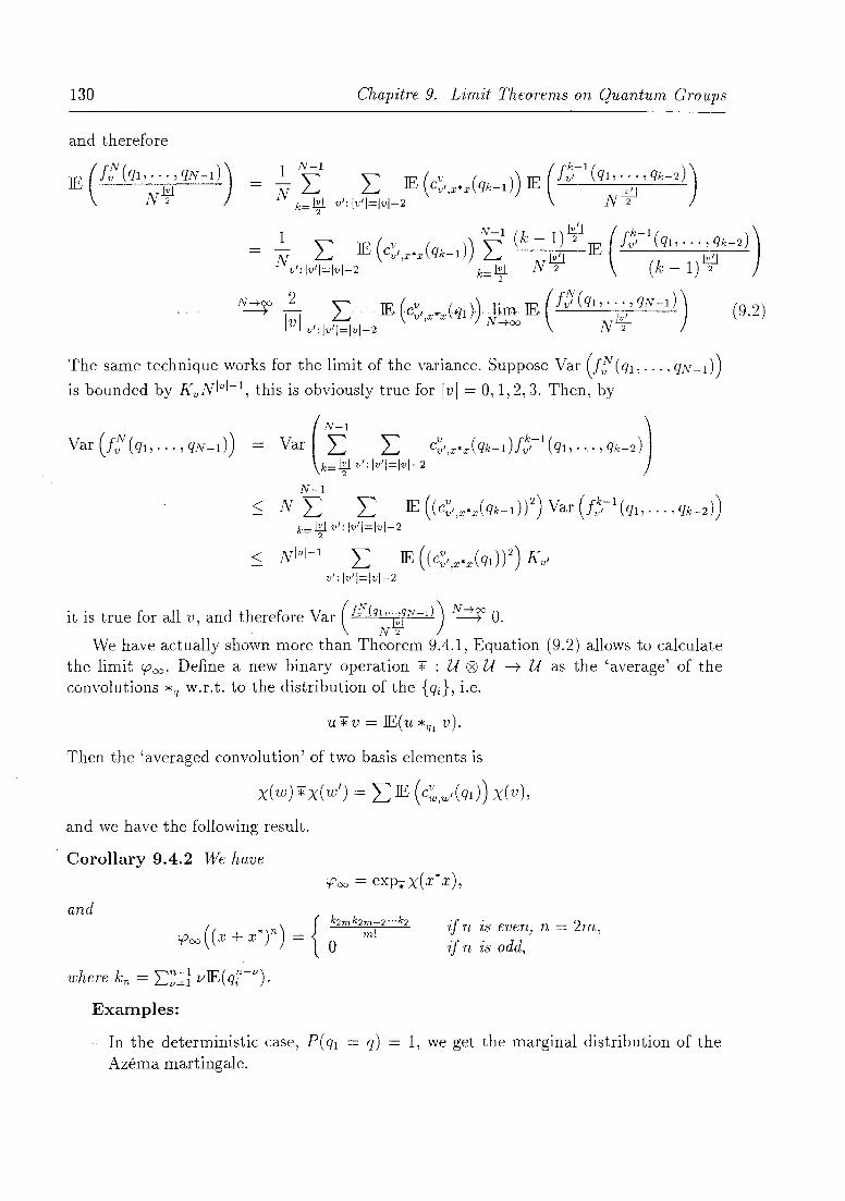
130 Chapitre 9. Limit Theoreins on Quantum Groups
and therefore
~ ~ "IE( v ( ))IE(f:'-1(ql, ... ,qk-2)) - N LJ L.J cv',x*x qk-l ~ k-l!1 v': Iv'I=lvl-2 N 2
- 2
~ " IE ( v ( )) ~l (k - 1)~ IE (f:,-l(ql, ... , qk-2)) N L...J cv',x'x qk-l L...J.l!j .l!j
v':lv'I=lvl-2 k=~ N 2 (k - 1) 2
N-+f ... ~ " ..... lE. (cv, .. ~~/l))' .lim JE.. (ftf(ql , .. ',' qN-d) Ivl L..:.J v,x x N-+oo N~
v': Iv'I=lvl-2 2
The same technique works for the limit of the variance. Suppose Var (J!;,(ql"" ,qN-d) is bounded by KvN1vl-l, this is obviously true for Ivl = 0,1,2,3. Then, by
N-l < N 1: L IE((c~"x.Aqk_d)2)Var(f:'-1(ql, ... ,qk_2))
k-l!1 v': Iv'I=lvl-2 - 2
< Nlvl-l L IE ((c~"x.x(ql))2) Kv' v': Iv'I=lvl-2
it is true for an v, and therefore Var (ft'(q~%fN-d) ~ O.
We have actually shown more than Theorem 9.4.1, Equation (9.2) allows to calculate the limit <POO' Define a new binary operation "* : U ® u -+ U as the 'average' of the convolutions *q w.r.t. to the distribution of the {qi}, i.e.
u"* v = IE( U *ql v).
Then the 'averaged convolution' of two basis elements is
and we have the following result.
Corollary 9.4.2 We have <POO = exp;;-x(x*x),
and <POO ((x + x*t) = { ~2mk2:!2 ... k2
where kn = L~;;;;i lIIE(qi- V ).
Examples:
if n is evenJ n = 2m, if n is odd,
- In the deterministic case, P(ql = q) = 1, we get the marginal distribution of the Azéma martingale.
(9.2)

9.5. Operator-limit theorems on bialgebras 131
- For Bernoulli, P(ql = 1) = p, P(ql = -1) = 1 - p, P E [0,1],
m-l
'Poo ((x + x*)2m) = II (1 + 2fLP) I-L=O
9. 5 Operator~ limit theorems- on bialgebras-
One can also try to formulate limit theorems where the normalization is done by linear operators, e.g. algebra or coalgebra homomorphism, instead of scalars, along the Enes of [JM93].
132 Chapitre 9. Limit Theorems on Quantum Groups
Chapitre 10
Classical Markov Processes from Quantum Lévy Pro cesses
Work in Progress
Résumé
We show how classical Markov processes can be obtained from quantum Lévy processes. It is shown that quantum Lévy processes are quantum Markov processes, and sufficient conditions for restrictions to subalgebras to remain quantum Markov processes are given. Then there exists a classical Markov process whenever we can restrict to a commutative subalgebra without loosing the quantum .Markov property[Küm88]. Several examples, including the Azéma martingale, with explicit calculations are presented. In particular, the action of the generator of the classical Markov process on polynomials and the moments of the classical process can be calculated using Hopf algebra duality.
133

134 Chapitre 10. Classical Markov Processes from Quantum Lévy Processes

10.1. Introduction 135
10.1 Introduction
It is an interesting question which quantum stochastic pro cesses admit classical versions, i.e. for what families of operators {Xi = jt(x)lt E I} there exists a classical stochastic process {Xt It E I} on sorne probability space (n, F, P) such that ail time-ordered moments agree, i.e.
for sorne fixed state iI? A famous example of a classical version of a quantum Lévy process is the the Azéma
martingale [Azé85, Eme89, Par90, Sch91, Sch93]. In this case there exists an element x such that the pro cess {Xi = jt(x)} is actually commutative, and thus it is clear that it is equivalent to a classical process.
We will use the theory of quantum Markov pro cesses to give weaker conditions that guarantee the existence of classical versions of Lévy process, and study examples.
In Section 10.2 we recall the definitions of quantum Lévy processes and quantum Markov processes, show that every quantum Lévy process is a quantum Markov process, and give conditions under which the restriction of a quantum Lévy process to a subalgebra remains a Markov process.
In the following section (Section 10.3) we study several examples, including the Azéma martingale and a symmetrized Poisson process, and show how Hopf algebra duality can be used for explicite calculations.
10.2 Classical versions of quantum Lévy processes
10.2.1 Quantum Lévy pro cesses
The definition of a Lévy pro cess {jstlO s S s t ST}, T E lR+ U {oo} on a (braided) *-bialgebra B over a quantum probability space (A, <1» is presented in Definition 2.5.1. For simplicity we will assume that B is a Hopf algebra, and that the process is given by {jt = jotlO S t ST}. Let us also assume that (A, <1» is the quantum probability space obtained as inductive limit from finite tensor products on B and the marginal distribution 'Pt = <1> 0 j, by the construction described in [Sch93, pp. 38-40] and in Section 4.8. For an interval l ç [0, T] we denote by AI the *-subalgebra of A generated by UTEI jT(B). For singletons {t} = [t, t] the algebra At = Alt.t] is isomorphic to B, and we have the isomorphisms Ts.t : As -7 At, Ts,t = j, 0 j;l.
10.2.2 From quantum Lévy to quantum Markov
We want to define conditional expectations PI : A -7 AI and show that a Lévy pro cess satisfies PIO,s](At) ç As for ail ° ::; s ::; t ::; T, i.e. that it is a quantum Markov process. Remember that in the finite tensor product via which the inductive limit is defined the factors correspond to increments. Consider an interval of the form [0, t]. Let Bigin be the 'approximation' of A corresponding to (SI, . .. , Sk, ... , sn), SI < ... < Sn, i.e. the entries

136 Chapitre 10. Classical Markov Processes from Quantum Lévy Processes
of the ith factor in the tensor product represent the Încrement during the interval [Si-l, Si]
(set 50 = 0). Let Sk = t. Then set
~0(e 0 'PSk+l-Sk) 0 (e 0 'Psn-Sn_l)
k times
In the inductive limit this defines an operator P[O,I] : A ---1- A[o,t].
Proposition 10.2.1 The operator p[O,t] is completêly positive and satisfies p[~,t] = P[O,I] and p[O,t](xyz) = XP[O,t)(y)z for aU x, z E A[o,t], Y E A, i.e. it is a conditional expectation.
Proof: The positivity follows immediately from the way p[~:r·,Sk. ... ,sn) is defined as a combinat ion of the identity map and the positive functionals ys,-Si_l' And the compatibility with the inductive limit, i.e. the compatibility with the maps j.,. follows from the fact that the functionals form a convolution semigroup. 1
P ... nnnsiti ..... n 102') fX!.e h,,,,,, P. J A'\ { A {~~ ~ll n,/ ~,/ -1-'/ '7': ~ (: If) /' -" /' ,'Tl) ..... '&'-1'- .I.V.L'U".U. -LV ... .bJ ,/J; IltUiUL-.L lO,sJ\.,/'""'\.t} .'::::= ".r\.s JUI UI,L v .::::: ~ .:::::: ~ .:::::: 1 i t.t. l.JtjU :::::: L :::::: 1. J is a quantum Markov process.
Proof: Since the one-dimensional distributions form a convolution semigroup, aIl p[~~~r",Sk>-",sn) for n ~ 2, 0 < Sk = S < Sn = t act in the same way on elements of At, namely p[~~r··sk, ... ,sn)IAt = js 0 (idB 0 yt-s) 0.6. 0 ft 1 , and therefore this is also true for p[o.s] lAt . In particular, it follows p[o,s](At ) ç As 1
10.2.3 From quantum Markov to classical Markov
vVe know (see e.g. [BKS96]) that for every quantum Markov process on a commutative * -algebra (e.g. the subalgebra generated by one self-adjoint element) there exists a classical version, i.e. a classical stochastic process that has the same (time-ordered) joint moments as the quantum Markov process. The quantum Markov property is sufficient (not necessary) for the joint density associated to the joint time-ordered moments to be positive, and then the classical process exists by Kolmogorov's construction.
Thus we need to look for self-adjoint elements of 8 who generate a subalgebra such that the restriction of the quantum Lévy process to this algebra remains Markov. Take x E 8, x'" = x, and denote the * -algebra generated by x by 8 x .
vVe give two criteria that guarantee that the restriction of {Jt} to 8 x remains Markov.
Proposition 10.2.3
(a) Let 8 0 be a *-subalgebra of 8. If .6.(Bo) ç Bo 0 8 (i.e. Ba is a right coideal), then the restriction {jtIBo } to Ba of every Lévy process {Jt} on B is a quantum Afarkov process.
(b) Let L be the generator of {jt}, x E B self-adjoint. Then the restriction of {Jt} to BX is a quantum lvfarkov ptocess if and only if p( L) = (id 0 L) 0 .6. leaves BX invariant, i. e. if p(L)(BX) ç BX.
10.3. Examples of classical versions of Lévy processes on IRq * IR1jq 137
10.3 Examples of classical versions of Lévy processes
on IRq * IR1jq
Let us first consider the bialgebra that leads to the Azéma martingale (cf. [Sch91, Sch93]). It can be viewed as the free product of the braided line with its dual. As an algebra it is generated by one element a and its adjoint a*, with no relations between a and a*. Thus the set B = {1, a, a*, aa, aa", a*a, a*a*, ... } of aU words in the two letters a, a* forms a basis of IRq * IRljq. The coproduct and counit are defined as
6(a)=a+a', 6(a*) = a* + a*', s(a) = s(a*) = 0
on the generators and extended as algebra homomorphisms (Notation: a(*) = aH ® 1, aH' = 11;>9 a(*)). Here the algebra structure of (IRq * IRljq)®(IRq * IRljq) is determined by the braid relations
a' a = qaa', *' *' a a = qaa , I:$: -1 * aa =q a a *' * -1 * xl aa=q aa,
w here we assume q E IR \ { 0 } . vVe need to construct the dual U of IRq * IRljq. For q = 1 this is the shuffie algebra, see
e.g. [SS93, Section 3.8]. In the general case the dual might be called a q-shuffie algebra, the formulas of the shuffie algebra only have to modified by sorne q-dependent combinatorial coefficients.
A functional on IRq * IRljq is determined by its action on the basis chosen above, i.e. on the 'words' in a, a*. Thus it can be written as
U = L CxX, xEX
where X is the dual basis of B, i.e. the set of an words in two letters (x, x*), and Cx E Œ. As dual of a coalgebra this is an algebra, and if we restrict to fini te linear combinations, then it is also a coalgebra, and the dual pairing
< X,p >= { ~ if X,p are identical modulo the substitution a H x, a* H x*, else,
X EX, (3 E B, is still non-degenerate. The coproduct of a word in x, x* is just the sum over the different ways to split the
word in two, i.e. for a word with n letters there are exactly n + 1 terms. Thus we have e.g. 6x = x@1+I®x,6x* = x*®1+1®x*, or 6xx*x = xx*x®l+xx*@x+x@x*x+l®xx*x.
To compute the product 12 of two basis elements Xl, X2 in the q-shuffie algebra, we have to look at an the ways in which the first word Xl can be 'shuffied' into the second. The first term 1S simply the concatenation XIX2. Now we form aIl combinations of the letters of Xl and X2 where the order of the letters of Xl (and X2, resp.) remains unchanged, and
12. Here we used the convention < u· v, p >= 2:: < u, p(1) >< V, p(2) >, i.e. we defined the dual pairing of the tensor product algebra with the fiip automorphism 7: < " . >0= « " . > Q9 < " . » 0 (id Q9 70 id).

138 Chapitre 10. Classical Markov Processes jrom Quantum Lévy Processes
add a factor q every time an x (from xd is moved to the right across a let ter of X2, and a factor q-l every time an x* (from Xl) is moved to the right across a letter of X2. Thus, e.g.
x· x xx + qxx = (1 + q)xx, xx* + qx*x, x*· x - x*x +'q-Ixx*,
x· x* x*· x* x*x* + q-Ix*x* = (1 + q-l )x*x*,
or
,-"-..
xx*· xx* '-v-'
,-"-.. ...........-.. ,-"-.. ~ ~ ,-"-..
xx* x:r*+q:71 xxx* x!' + xxx"f x* +q=2 xxx* x* +q-l xxx-*'x* + xx* xx* '-v-' ~ ---..........- '-v-' '--v-" '-v-'
_ 2xx*xx* + (1 + 2q-1 + q-2)xxx*X*.
WARNING:xx, xx*, xx*xx*, etc. means concatenation, in this section the multiplication in U is always indicated by a dot.
The dual action or right regular representation 13 p(x) = (id®X)o~ of U eliminates the letters corresponding to those of X, ifthey are in the same order, with possibly additional letters in between, and adds a factor q (q-l, resp.) for every letter to the left of an a (a*, resp.) that is suppressed. E.g., on an element ala2···an E IRq * IR1/ q, \vith ai E {a,a*}
for i = 1, ... ,n, i-l v q al' .. ai'" an
i:ai=a*
p( xx*) : al ... an J--1-i-j+l v v q al··· ai··· aj···an·
i<j: ai=a, aj=a*
10.3.1 The Azéma martingale
If we choose the generator L = CIXX* + C2X*X, with Cl, C2 E lR+, then the classical version of jt(a + a*) is the Azéma martingale Mt (cf. [Sch91, Sch93]), i.e. the (finite) joint moments of {jt(a + a*);t E lR+} agree with those of the Azéma martingale: IE(M~! ... M4k) = cp ((jt! (a + a*)t! ... (jtk(a + a*)tk) for aH t l , .. ·, tk E IR+, nI, ... ,nk E IN, k E IN. In order to find the generator of the Azéma martingale (as a classical Markov process) and to compute the moments, we need to know how L acts on the subalgebra generated by z = a + a*.
Proposition 10.3.1 (Leibnitz formulas). Let j = Lk=O jkzk with jk E Πand z =
a + a*. Then
p(x)(zJ)
p(x*)(zJ)
p(xx*)(zJ)
p(x*x)(zJ)
j + qzp(x)j,
j + q-l zp(x*)j,
p(x*)j + zp(xx*)j,
p(x)j +zp(x*x)j.
13. i.e. p(X)/3 = « " . > 0id) 0 (id 0 r) 0 (id 0 ~)(X 0 /3) for an X EU, /3 E A.
10.3. Examples of classical versions of Lévy processes on IRq * IRl/q 139
Proof: This follow from the braided version of Equation (2.1). 'vVe have p(u)(aj3) = I: a(11.(id0u(1))(W( a(2)0p( U(2l)j3)) (where we used Sweedler's notation for the coprodud). Applying the braid relations and recalling that z, x, x* are primitive, while ~(xx*) =
xx* 0 1 + x 0 x* + 1 0 xx*, Ll(x*x) = x*x 01 + x* 0 x + 1 0 x"'x, we get the desired formulas. 1
Setting f = zn, we obtain recurrence relations that allow us to determine the operators on polynomials in z,
p(x) : zn 1---» qn zn =} (p(x)f)(z) <5 f(z) = f(qz)-f(z) q z(q-l)
p(x*) : zn 1---» (q-l )nzn =} (p(x)f)(z) S / fr ,:,) - f(q-lz)-f(z) l q ,~ - z(q-l-1)
{ (q-l)n-n n-2
n ~ 2, 0Ifqf(z)-fl(Z) p(xx*) : zn 1 Z (p(xx*)f)(z) 1---» q -1 =}
0 n = 0,1 z(q-l-1)
{ qn-n n-2 n ~ 2,
p(x*x):zn 1---» q-1 Z
=} (p(xx*)f)(z) oqf(z)- fl(Z)
0 n = 0,1 - z(q-l)
for q 1- 1, and p(x)f = p(x*)f = J', p(xx*)f = p(x*x)f = ~f" for q = 1. Using these operators to calculate the Appell polynomials
h (_·t) - etp(L)".n n 4, - "'" ,
we can aiso calculate the moments of the Azéma martingale, IE( J'vIt) summarize the results in the following theorem.
Theorem 10.3.2 Let (jt)tElR+ be the quantum Lévy process on IRq * lR l / q with generator L = CIXX* + C2X*X, Cl,C2 E IR+! and (Nlt )tElR+ the classical version of jt(a + a*) (l:.e. the Azéma martingale). Then the generator La+a * of Aft (as a classical A1arkov process) is given by
L f( 7) - z(q-1) { C20qf(z)-qCjOl(qf(z)-(C2-QCj )fl(Z)
a+a* ~ - C]~C? f"(z) q = 1
on polynomials f(z) = I:~=o fk Zn ) fo, fI,"" fn E Œ. The moments of this process are
n = 2m even, n odd,
where k = C (q-l)n-n + C qn-n for q -1- 1 and kn = (Cl + C2)n(nz-1) for q = 1. n 1 q-l-1 2 q-1 J' r) J'
10.3.2 Other pro cesses on lRq * lR1/qo
If we want to obtain other classical pro cesses we can either change the quantum process, i.e. choose a different generator, or use a different commutative subalgebra of IRq * IRl/q that satisfies the conditions discussed in Subsection 10.2.3. Let us briefly look at the second possibility. We need an element of u E B = IRq*IRl/q such that LlB" ç B0(IRq*
IR I / q). A possible choice is u = a*a + qaa*. In fad, Llun = I:~=o ( ~ ) U V ( u')n-v, so that
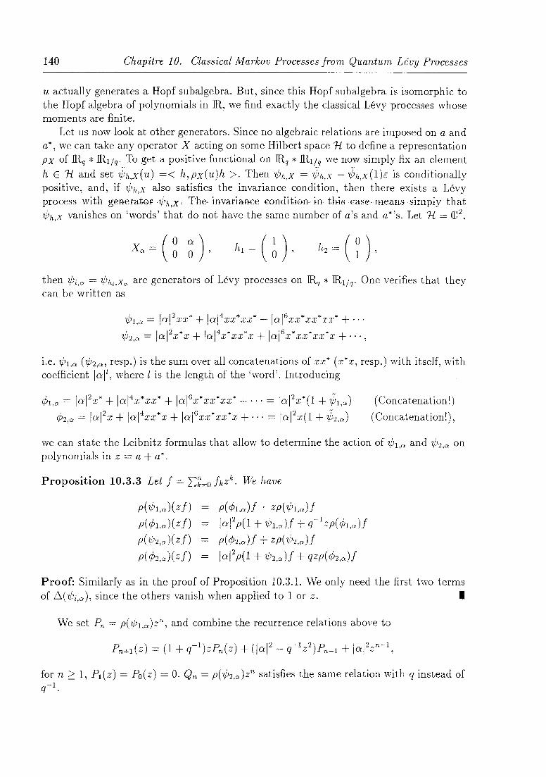
140 Chapitre 10. Classical Markov Processes from Quantum Lévy Processes
u actually generates a Hopf subalgebra. But, since this Hopf subalgebra is isomorphic to the Hopf algebra of polynomials in lR, we find exactly the classical Lévy pro cesses whose moments are finite.
Let us now look at other generators. Since no algebraic relations are imposed on a and a*, we can take any operator X acting on sorne Hilbert space 1l to define a representation Px of 1Rq * 1R1/q. To get a positive functional on 1Rq * lR l / q we now simply fix an element h E 1l and set ~h,X(U) =< h,px(u)h >. Then 1/;h,X = ~h,X - ~h,X(1)é is conditionally positive, and, if 1/;h,X also satisfies the invariance condition, then there exists a Lévy process with generatm1/;h,x. The-invariance €Ondition-·in this€ase-means.simply that 1/;h,X vanishes on 'words' that do not have the same number of a's and a*'s. Let 1l = (1;2,
then 1/;i,O/ = 1/;h;,Xa are generators of Lévy pro cesses on lRq * lR1/q. One verifies that they can be written as
1/;1,0/ = lal 2xx* + laJ 4xx*xx* + JaI 6 xx*xx*xx* + .. . 1/;2,0/ = /a/ 2x*x + /aI 4 x*xx*x + laI 6 x*xx*xx*x + ... ,
i.e. 1/;1,0/ (1/;2,0/, resp.) is the sum over aIl concatenations of xx* (x*x, resp.) with itself, with coefficient lal l , where l is the length of the 'word'. lntroducing
1>1,0/ = lal 2x* + laI 4 x*xx* + laI 6 x*xx*xx* + ... = laI 2x*(1 + ~1,0/) 1>2,0/ = lal2x + lal 4 xx*x + la/ 6 xx*xx*x + ... = lal 2x(1 + ~2,0/)
(Concatenation! )
(Concatenation!) ,
we can state the Leibnitz formulas that allow to determine the action of 1/;1,0/ and 1/;2,0/ on polynomials in z = a + a*.
Proposition 10.3.3 Let f = 2:k=o fkZk. We have
p( 1/;1,0/) (z f)
p( 1>l,O/)(Zf)
p( 1/;2,Ct) ( z f) -
p( 1>2,0/)( z f)
P(1)l,O/)f + ZP(1/;l,O/)f
lal 2 p(l + 1/;1,0/)f + q-1 zp( 1>l,O/)f
p( 1>2,0/)f + zp( 1/;2,0/)f
la/ 2 p(l + 1/;2,0/)f + qzp( 1>2,0/)f
Pro of: Similarl'yas in the proof of Proposition 10.3.1. vVe only need the first two terms of l:i( 1/;i,O/) , since the others vanish when applied to 1 or z. •
We set Pn = p( 1/;1,0/) Zn , and combine the recurrence relations above to
for n ~ 1, P1(z) = Po(z) = O. Qn = p(1/;2,0/)Zn satisfies the same relation with q instead of -1 q .

10.3. Examples of classical versions of Lévy processes on IRq * IRl/q 141
This recurrence relation allows to calculate the Qn, for the first ten we get (with Maple)
Q( 0, x): = 0
Q( 1, x ): = 0
Q( 2, x ): = lal2
Q( 3, x): = (21al2 + q lal2) x
Q( 4, x)-:- = t3 1012 +2 q lal2 + q21(12) x 2-+ 1001 4
Q( 5, x): = (4 lal2 + 2 q2 lal 2 + q31al2 + 3 q lal 2 ) x3 + (3 lal4 + 2 q lal4) x
Q( 6, x): =
(3llal2 + 51al 2 + 4 q lal2 + q41al2 + 2 q31(12) x 4 + (61a14 + 6 q lal4 + 3 q21( 14) x 2 + lal6
Q( 7, x): = (61a12 + ,5 q JaJ2 + 4 q21al 2 + 3 q3 !a!2 + q51al 2 + 2 q4Ia/ 2) x5
+ (12q lal4 + 4q31al4 + 10 lal4 + 9q21(14) x3 + (3q lal6 + 41(16) x
Q( 8, x ): = (q61a12 + 6 q lal2 + 3 q41aJ2 + 2 q51al2 + 4 q31al2 + 5 q21al 2 + 71( 12) x6
+ (5 q41al4 + 151al4 + 12 q31al4 + 18 q21al4 + 20 q lal4) x4
+ (6llal 6 + 12 q lal6 + 10 lal6) x2 + lal8
Q(9,x): = (5 q3 lal2 + 81al 2 + 4q41al 2 + 3 q51al 2 + 2llal2 + 6q21aJ2 + q71al2 + 7 q lan x7
+ (211a14 + 6 q51al4 + 15 q41al4 + 30 q lal4 + 24llal4 + 30 q21 ( 14) x 5
+ (30 q lal6 + 24 q21al6 + 20 lal6 + 10 q31(16) x3 + (4 q lal8 + 51(18) x
Q( 10, x) : =
(8 q lal2 + 4 q51al2 + 6 q31al2 + 5 q41al 2 + 2 q71al2 + 91al 2 + 3 q6Jal 2 + 7 q21al 2 + q81(12)
x8 + (28 lal4 + 18 q51al4 + 40 q31al4 + 30 q41al4 + 42 q lal4 + 7 q61al4 + 45 q2JaJ4) x6
+ (60 q21al6 + 40 q31al6 + 15 q41al6 + 351al6 + 60 q lan x4
+ (15 1a18 + 10 q21al8 + 20 q laiS) x 2 + lallO
For q = 1 these polynomials are ~{(x + Jal)n + (x - Jal)n - 2xn, i.e. the generator is a difference operator, Lf(x) = Hf(x + lai) + f(x - lai) - 2f(x)}, and the pro cess is a difference of two Poisson processes with jumps of size lai and same intensity. From these we can build any symmetric compound Poisson process by taking the generator

142 Chapitre 10. Classical Markov Processes from Quantum Lévy Processes
Lp, = IlR 7,Ul,O'dp(O:') , and thus we have 'q-analogues' of symmetric compound Poisson pro cesses at hand. _
If we replace Pn by Pn = Pn + zn, then we get a homogeneous recurrence relation of the form Pn+l = aPn + bPn-l, with a = (1 + q-l)Z and b = (10:'1 2 - q-l z2). The solution of this relation with Po = 1, Pl = Z, is given by
and similarly for the Qn, just replace q by q-l.
Theorem 10.3.4 Let (jt)tElR+ be the Lévy process with generator 7,U2,0'. Then the generator of the associated classical Nfarkov process acts on polynomials as

[Abe80]
[ADT94J
[AFL82]
[ALV94]
[And69]
[ASvV88]
[Azé85]
[Ba185J
Bibliographie
Abe (E.). - Hopf Algebras. - Cambridge~ Cambridge Unversity Press~ 1980.
Andruskiewi tsch (N.), Devoto (J.) et Tiraboschi (A.). - Quantum Heisenberg groups and Sklyanin algebras. Lett. Math. Phys., vol. 31, 1994, pp. 167-177.
Accardi (L.), Frigerio (A.) et Lewis (J.T.). - Quantum stochastic processes. Publ. RIJvIS, vol. 18, 1982, pp. 97-133.
Accardi (L.j, Lu ('{.G.) et Volovich (1.). - Non-commutative (quantum) probability, master fields and stochastic bosonization. Preprint Centro V Volterra 198-94, 1994.
Anderson (R.F.V.). - The Weyl functional calculus. J. Funct. Anal., vol. 4, 1969, pp. 240-267.
Accardi (L.), Schürmann (M.) et vValdenfels. (W.v.). - Quantum independent increment pro cesses on superalgebras. Math. z., vol. 198, 1988, pp. 451-477.
Azéma (J.). - Sur les fermés aléatoires. In: Séminaire de Probabilités XIX, Strasbourg 1983/1984, éd. par Azéma (J.) et Yor (M.). - Springer, 1985.
Baldi (P.). - Unicité du plongement d'une mesure de probabilité dans un semÎgroupe de convolution gaussien. cas non-abélien. Math. z., vol. 188, 1985, pp. 411-417.
[BCG+94] Bonechi (F.), Celeghini (E.), Giachetti (R.), Pere na (C. l'v1.) , Sorace (E.) et Tarlini (M.). - Exponential mapping for non-semisimple quantum groups. J. Phys. A: Alath. Gen., vol. 27, 1994, pp. 1307-1315.
[BH9.5] Bloom CW.R.) et Heyer (H.). - Harmonic Analysis of Probability Measures on Hypergroups. - Berlin, de Gruyter, 1995, de Gruyter Studies in A1athematics, volume 20.
[Bia93] Biane (P.). - Ecole d'été de Probabilités de Saint-Flour, chap. Calcul stochastique non-commutatif. - Berlin, Springer-Verlag, 1993, Lecture Notes in Alath., volume 1608.
[BKS96] Bozejko (M.), Kümmerer (B.) et Speicher (R.). - q-Gaussian processes: Noncommutative and classical aspects. funct-an/9604010, 1996.
143
144 Bibliographie
[BL96] Bucchianico (A. Di) et Loeb (D.E.). - Operator expansion in the derivative and multiplication by x. Integral transforms and special functions, vol. 4, nl-2, 1996, pp. 49-68.
[BM93] Baskerville (W. K.) et Majid (S.). - The braided Heisenberg group. J. l11ath. Phys., vol. 34, 1993, pp. 3588-3606.
[BN71 J Butzer (P.L.) et Nessel (R.J.). - Fourier Analysis and Approximation, Vol. 1. - Birkhauser, 1971, NIathematische Reihe, volume 40.
[BS91] Bozejko (M.) et Speicher (R.). - An example of generalized Brownian motion. Commun. NIath. Phys.) vol. 137, 1991, pp. 519-531.
[CP95] Chari (V.) et Pressley (A.). - A guide to quantum groups. - Cambridge University Press, 1995.
[DHL91 J Doebner (H. D.), Hennig (J. D.) et Lücke CW.). - Mathematical guide to quantum groups. In: Proceedings of Quantum Groups Conference held in Clausthal ;~ tnQ9 ('~~;~n~~ T ~n+".~~ !\T~-I-~~:~ Dh"s C"yyn 0<.-1 ---- r\ __ 1 ___ -. (TT" \ et TnT b" .LoJu-, 01" ",yu DctAU/C- iyu~c-;:, Mil IV . v lU, eu. Pdr lJOeUller ~n. 0.) c en-nig (J. D.). - 1991.
[Dri87] Drinfeld (V. G.). - Quantum groups. In: Proceedings of the International Congress of 1l1athematicians, Berkeley 1986. American Mathematical Society. - 1987.
[Eme89] Emery (M.). - On the Azéma martingales. In: Séminaire de Probabilités XXIII. - Springer, 1989.
[EMO+54] Erdelyi (A.), Magnus (\V.), Oberhettinger (F.), Tricomi (F.G.) et Bateman (H.). - Tables of Integral Transforms, Vol. 2. - McGraw-Hill, 1954, Bateman manuscript project.
[Fei87] Feinsilver (P.). - Generalized convolutions and probability theory based on the q-Heisenberg algebra. In: Proc. First vVorld Congr. Bernoulli Soc. pp. 729-741. - VNU Science Press, 1987.
[FF] Feinsilver (P.) et Franz (U.). - Brownian motion on the affine group and generalized Gegenbauer polynomials. - in preparation.
[FFS95] Feinsilver (P.), Franz (U.) et Schott (R.). - Duality and multiplicative processes on quantum groups. In: Proceedings of the International Conference on "Nonlinear, Deformed and Irreversible Quantum Systems", éd. par Doebner (H.D.), Dobrev (V.) et Nattermann (P.). pp. 462-468. - World Scientific, 1995.
[FFS97] Feinsilver (P.), Franz (U.) et Schott (R.). - Duality and multiplicative processes on quantum groups. J. Theor. Prob., vol. 10, n3, 1997, pp. 795-818.

145
[FG93] Fronsdal (C.) et Galindo (A.). - The dual of a quantum group. Lett. Jvfath. Phys., vol. 27, 1993, pp. 59-7I.
[FNS96] Franz (U.), Neuenschwander (D.) et SchoH (R.). - Gauss laws in the sense of Bernstein and uniqueness of embedding into convolution semigroups on quantum groups and braided groups. - Prépublication n 96/n° 31, Institut Elie Cartan, Nancy, 1996. to appear in Probability Theory and Related Fields.
[FS89aJ Feinsilver (P.) et Schott (R.). - An operator approach to processes on Lie groups: In: Lecture Notes in 1\1Jathemafics, Vol. 1391. Conference Proceedings, 'Probability Theory on Vedor Spaces', Lancut 1987, pp. 59-65. - New York, 1989.
[FS89b J Feinsilver (P.) et Schott (R.). - Operators, stochastic pro cesses , and Lie groups. In: Lecture Notes in Alathematics,. Vol. 1319. Oberwolfach Conference, 'Probability Measures on Groups', pp. 75-85. - New York, 1989.
[FS92] Feinsilver (P.) et Schott (R.). - Appell systems on Lie groups. J. Theor.
[FS96a]
fFS96b]
[ Gie95]
[Gui95]
[Haz77]
[Hey77]
[Jim85]
[Jim86]
[JM93)
Probability, vol. 5, 1992, pp. 251-281.
Feinsilver (Ph.) et Schott (R.). - Aigebraic Structures and Operator Calculus,. Volume III: Representations of Lie Groups. - Kluwer, 1996.
Franz (U.) et Schott (R.). - Diffusions on braided spaces. - Prépublication n 96/no 4, Institut Elie Cartan, Nancy, 1996. ASI-TPA/28/95.
Giering (M.). - Representations and Differential Equations on the Classical Domains of Type IV, using Coherent State l\IIethods and a New Formulation of Berezin Qitantization for 50(n, 2)/ SO(n )050(2). - Thèse de PhD, Southern Illinois University at Carbondale, Dept. of Molecular Science, 1995.
Guichardet (A.). - Groupes quantiques. - Paris, InterÉdition/CNRS Éditions, 1995.
Hazod (W.). - Stetige Faltungshalbgruppen von WahrscheinlickeitsmajJenund erzeugende Distributionen. - Berlin, Springer-Verlag, 1977, Lecture Notes in .Math., volume 595.
Heyer (H.). - Probability measures on locally compact groups. - Berlin, Springer-Verlag, 1977.
Jimbo (M.). - A q-difference analogue of U(g) and the Yang-Baxter equation. Lett. Math. Phys., vol. 10, 1985, pp. 63-69.
Jimbo (M.). - A q-analogue of U(gl(N + 1)), Hecke algebra, and the YangBaxter equation. Lett. Math. Phys, vol. 11, 1986, pp. 247-252.
Jurek (Z.J.) et Mason (J.D.). - Operator-Limit Distributions in Probability Theory. - \rViley, 1993.

146 Bibliographie
[JS91a] Joyal (A.) et Street (R.). - The geometry of tensor calculus 1. Adv. j'lrfath., vol. 88, nI, 1991, pp. 55-112.
[JS91b] Joyal (A.) et Street (R.). - An introduction to Tannaka duality and quantum groups. In: Category theory) Proc. Int. Conf.J Como/ltaly 1990, éd. par Carboni (A.), Pedicchio (M.C.) et Rosolini (G.). pp. 413-492. - Springer, 1991. Lect. Notes in Math. 1488.
[JS93] Joyal (A.) et Street (R.). - Braided tensor categories. Adv. Math., vol. 102, n 1, 1993, pp. 20~78.
[Kas95] Kassel (Ch.). - Quantum Groups. - Springer, 1995, Graduate texts in mathematies, volume 155.
[KM94] Kempf (A.) et Majid (S.). - Algebraic q-integration and Fourier theory on quantum and braided spaces. J. A1ath. Phys., vol. :35, 1994, pp. 6801-6837.
[Ko091] Koornwinder (T.H.). - Positive convolution structures associated with quantum groups. In: 10th Oberwolfach Conference) 'Probability Measures on Groups '. - New York, 1991.
[Ko094] Koornwinder (T.H.). - General compact quantum groups) a tutorial. - Report n 94-06, Dept. of Math. and Comp. Sci., Univ. of Amsterdam, 1994. hepthj9401114.
[Ko095] Koornwinder (T.H.). - Minicourse "special functions and q-commuting variables". In: Workshop on "Special functions, q-series and related topies". Fields Institute, Toronto, Canada, 12-23 June 199. - 1995.
[K üm88] K ümmerer (B.). - Survey on a theory of non-commutativ stationary Markov processes. In: Quantum Probability and Applications III, éd. par Accardi (L.) et Waldenfels (W.v.), pp. 228-244. - Springer, 1988.
[LM95J Leeuwen (H.van) et Maassen (H.). - A q-deformation of the Gauss distribution. J. Math. Phys., vol. 36, 1995, pp. 4743-4756.
[Mac71] MacLane (S.). - Categories for the working mathematician. - Springer, 1971, Graduate texts in mathematics, volume 5.
[Maj90] Majid (S.). - Quasitriangular Hopf algebras and Yang-Baxter equations. Int. J. j'lyfod. Phys. A, vol. 5, nI, 1990, pp. 1-91.
[Maj92] Majid (S.). - C-statistical quantum groups and Weyl algebras. J. Afath. Phys., vol. 33, 1992, pp. 3431-3444.
[Maj93a] Majid (S.). - Beyond supersymmetry and quantum symmetry (an introduction to braided groups and braided matrices). In: Quantum Integrable Statistical Models and Knot Theory, éd. par Ge (M.L.) et Vega (H.J.). pp. 231-282. -World Scientific, 1993.

147
[Maj93b] Majid (S.). - Braided momentum in the q-Poincaré group. J. Math. Phys., vol. 34, 1993, pp. 2045-2058.
[Maj93c] Majid (S.). - Free braided differential calculus, braided binomial theorem, and the braided exponential map. J. Math. Phys., vol. 34, 1993, pp. 4843-4856.
[Maj93d] Majid (S.). - Quantum random walks and time-reversal. Int. J. Mod. Phys., vol. 8, 1993, pp. 4521-4545.
[Maj94] Majid{S. r. - Quanturn·d0Uhle-as quantum mechanie<'i.I Geom. Phys., vol. 13, 1994, pp. 169-202.
[Maj95a] Majid (S.). - *-Structures on braided spaces. J. Math. Phys., vol. 36, 1995, pp. 4436-4449.
[Maj95b] Majid (S.). - Foundations of quantum group theory. - Cambridge University Press, 1995.
[Maj95e] Majid (S.). - Quasi-* structure on q-Poincaré algebras. to appear in J. Geom. Phys., 1995. - q-alg/95030l4.
[Maj96] Majid (S.). - Introduction to braided geometry and q-Minkowski space. In: Proc. School 'Enrico Fermi' CXXVlI. pp. 267-348. - lOS Press, 1996.
[MeK69] McKean (H.P.). - Stochastic integrals. - Academie Press, 1969.
[Mey93] Meyer (P.-A.). - Quantum Probability for Probabilists. - Berlin, Springer, 1993, Lecture Notes in Math., volume 1538.
[MM93] Manko (V.L) et Mendes (R. Vilela). - q-deformed Brownian motion. Phys. Lett. A, vol. 180, 1993, pp. 39-42.
[MRP94] Majid (S.) et Rodrîguez-Plaza (M. J.). - Random walk and the heat equation on superspace and anyspace. J. Math. Phys., vol. 35, 1994, pp. 3753-3760.
[NeI66] Nelson (E.). - Derivation of the Schrodinger equation from Newtonian mechanies. Phys. Review, vol. 150, 1966, pp. 1079-1085.
[Neu93] Neuenschwander (D.). - Gauss measures in the sense of Bernstein on the Heisenberg group. Probability and Mathematical Statistics, vol. 14, 1993, pp. 253-256.
[Neu96] Neuensèhwander (D.). - On the uniqueness problem for continuous convolution semigroups of probability measures on simply connected nilpotent Lie groups. - submitted, 1996.
[NRS96] Neuenschwander (D.), Roynette (B.) et Sehott (R.). - Characterization of Gauss measures on nilpotent Lie groups and symmetric spaces. - Prépublication n96/n° 27, Institut Elie Cartan, Nancy, 1996.

148 Bibliographie
[NRS97] Neuenschwander (D.), Roynette (B.) et Schott (R.). - Characterizations of Gaussian distributions on simply connected nilpotent Lie groups and symmetric spaces. C. R. Acad. Sei. Paris, vol. 324, 1997, pp. 87-92.
[NS96] Neuenschwander (D.) et Schott (R.). - A note on domains of attraction for q-transformed random variables. - Prépublication n96/no 11, Institut Elie Cartan, Nancy, 1996. accepted for publication in Probability and Mathematical Statistics.
[Obe90] Oberhettinger (F.). - Tables of Fourier Transforms and Fourier Transforms of Distributions. - Springer, 1990.
[Pap94] Pap (G.). - Uniqueness of emhedding into a Gaussian semigroup on a nilpotent Lie group. Arch. Math., vol. 62, 1994, pp. 282-288.
[Par90] Parthasarathy (K.R.). - Azéma martingales and quantum stochastic calcul us. In: Proc. R.C. Bose Memorial Symposium, éd. par Bahadur (R.R.). - Wiley Eastern, 1990.
[Par92] Parthasarathy (K.R.). - An Introduction to Quantum Stochastics. - Birkhiiuser, 1992.
[RTF90] Reshetikhin (N. Yu.), Takhtadzhyan (L. A.) et Faddeev (1. D.). - Quantizatian of Lie groups and Lie algebras. Leningrad Math. J., vol. 1, nI, 1990, pp. 193-224.
[Sch91] Schürmann (M.). - The Azéma martingales as components of quantum independent increment processes. In: Séminaire de Probabilités XXV, éd. par Azéma (J.), Meyer (P.A.) et Yor (M.). - Springer, 1991.
[Sch93] Schürmann (M.). - White Noise on Bialgebras. - Berlin, Springer-Verlag, 1993, Lecture Notes in Mathematics, volume 1544.
[Sch95a] Schürmann (M.). - Direct sums of tensor products and non-commutative independence. J. Funct. Anal., 1995.
[Sch95b] Schürmann (M.). - Non-commutative probability on algebraic structures. In: Proceedings of XI Oberwolfach Conference on Probability Measures on Groups and Related Structures, éd. par Heyer (H.). pp. 332-356. - World Scientific, 1995.
[Sie73] Siebert (E.). - Über die Erzeugung von Faltungshalbgruppen auf beliebigen lokalkompakten Gruppen. Math. Z., vol. 131, 1973, pp. 313-333.,
[Sie81] Siebert (E.). - Fourier analysis and limit theorems for convolution semigroups on a locally compact group. Adv. Math., vol. 39, 1981, pp. 111-154.
[Ske94] Skeide (M.). - The Levy-Khintchine formula for the quantum group SU,(2). - Thèse de PhD, Univ. Heidelberg, Naturwiss.-Math. Gesamtfak., 1994.

149
[Spe] Speicher (R.). - Universal products. - preprint.
[Spe92] Speicher (R.). - A non-commutative centrallimit theorem. Math. Z., vol. 209, 1992, pp. 55-66.
[SS93] Shnider (S.) et Sternberg (S.). - Quantum Groups: from Coalgebras ta Drinfeld Aigebras, a Guided Tour. - International Press, 1993, Graduate texts in mathematical physics, volume 002.
[SW93] Speicher CR.) et Woroudi (R .. ).- Boolean cOllvolution.- preprillt, 1993.
[Swe69] Sweedler (M. E.). - Hopf Aigebras. - New York, Benjamin, 1969.
[VDN92] Voiculescu (D.), Dykema (K.) et Nica (A.). - Free Random Variables. - AMS, 1992.
[Wey31] Weyl (H.). - The Theory of Groups and Quantum Mechanics. - London, Methuen, 1931. reprinted by Dover Publications, 1950.
[Wig32] Wigner (E.). - On the quantum corrections for thermodynamic equilibrium. Phys. Rev., vol. 40, 1932, pp. 749-759.
[Wor87] Woronowicz (S. L.). - Compact matrix pseudogroups. Commun. Math. Phys., vol. 111, 1987, pp. 613-665.
[Wor91] Woronowicz (S.L.). - New quantum deformation of SL(2, Cl. Hopf algebra level. Rep. Math. Phys., vol. 30, n2, 1991, pp. 259-260.
[Wor92] Woronowicz (S. L.). - Quantum SU(2) and E(2) groups. Contraction procedure. Commun. Math. Phys., vol. 149, 1992, pp. 637-652.
[WZ94] Woronowicz (S. L.) et Zakrzewski (S.). - Quantum deformations of the Lorentz group. The Hopf *-algebra level. Compas. Math., vol. 90, n2, 1994, pp. 211-243.

150 Bibliographie
W-independent, 12 W-invariant,13 *-bialgebra, 8
antipode, 7 Appel! system, 38, 60, 99 Azéma martingale, 138
bialgebra, 7 braided *-bialgebra, 11, 52 braided antipode, 11 braided bialgebra, 11 braided independent, 12 braided space, 48 braided tensor category, 11 braided tensor product algebra, 11 braiding, 10
classical version, 6 coalgebra, 7 cocommutative, 7 comodule, 10 conditional expectation, 136 continuous convolution semigroup, 82
density, 6 deterministic state, 81 diffusion, 56 Dirac law, 81 distribution, 5 dual pair, 8 dual representation, 8, 32
equivalent, 6 evolution equation, 16
Feynman-Kac formula, 35 Fokker-Planck-type equation, 103
Index
Gaussian convolution semigroups in the sense of Bernstein, 87
Gaussian functional in the sense of Bernstein, 73
Gaussian generator in the sense of Schürmann, 88
Gaussian quantum convolution semigroup, 91
hexagon axiom, 10 Hopf algebra, 7
independent, 12
Leibnitz formula, 8 Lévy process, 13
marginal distribution, 5 module, 9 monoidal category, 9
nilpotent Hopf algebra, 83
one-dimensional distribution, 5
pentagon axiom, 9 primitive, 8 pseudo-(W-)independent, 12 pseudo-diffusion, 56
quadratic functional, 88 quantum convolution semigroup, 82 quantum Markov process, 136 quantum probability space, 5 quantum random variable, 5 quantum stochastic process, 5 quasi-triangular, 10
regular representation, 8
state, 5
151

152
tensor category, 9 triangle axiom, 9
universal R-matrix, 10
weakly Gaussian convolution semigroup in the sense of Bernstein, 87
weakly Gaussian functional in the sense of Bernstein, 74
Weyl map, 102 Wigner density, 103
Index

3C-F9
........ ~ ,alHGf..t; . ...... ~ . <" ..
:~ -/// : ~Cy~ _______ ~ __________________________________________ __
"/ .
/'
Nom: FRANZ
Prénom: Uwe
DOcrORAT de l'UNIVERSITE HENRI POI~CARE, NANCY-I
en MATHEMATIQUES
Vu, APPROUVÉ ET PERMIS D'IMPRIMER
Nancy, le 23 JUIN 1997 tJ H f ~I ~ 1-
UNIVERSITÉ IIllill 'OIIiCAlÉ . NAIICY 1 24·30. rue llonnols B.P.3069 54013 Nancy cedex Tél: 83 32 81 81 Fax: 83 32 95 90
Adresse électronique: ________ ...:. .. [email protected]

Résumé
Ce mémoire est rélatif à l'étude des processus stochastiques sur les algèbres de Hopf. Ces algèbres jouent un rôle important en physique mathématique sous le nom groupes quantiques.
Une grande partie -de cette tl:ïèse est' consacrée à l'étude des processus de Lévy, c~àd des processus à accroissements indépendants et stationnaires, sur ces algèbres. Deux constructions, soit à partir d'un processus de Lévy classique, soit à partir d'une marche aléatoire quantique, sont proprosées. Ces processus sont ensuite étudiés à l'aide des représentations duales et de leurs systèmes d'Appell. En particulier, ceci a permis de démontrer une formule de Feynman-Kac et d'établir un lien étroit entre ces processus et des équations d'évolution sur les groupes quantiques.
Les représentations duales sont également utilisées pour donner des conditions suffisantes pour l'existence de versions classiques des processus de Lévy sur des bigèbres et pour les caractériser. Plusieurs exemples, y compris la martingale d'Azéma, sont traités en détail.
Un autre thème central de ce travail est la caractérisation des lois de Gauss au sens de Bernstein. Il est montré comment les fonctionnelles ainsi que les semi-groupes de convolution sur des algèbres de Hopf qui satisfont l'analogue de la propriété de Bernstein peuvent être calculés. Il est aussi démontré que le plongement d'une fonctionnelle normée infiniment divisible dans un semi-groupe de convolution continu sur un groupe quantique nilpotent ou sur un groupe tressé nilpotent est unique.
Finalement, plusieurs théorèmes limites (loi des grands nombres, théorème de la limite centrale,- etc.) sur les groupes quàntiques sont présentés. '
Mots-clés: Processus de Lévy s~! des bigèbres, théorèmes limites
Abstract
In this thesis stochastique processus on Hopf algebras are studied. These algebras, aIso known under the name quantum group, play in important role in mathematical physics.
A major part of this work is concerned with Lévy processes, i.e. processes with stationary and independent increments. Two construction are proposed, one starts from a classical Lévy process, the other one uses quantom random walks. These processes are then studied with the help of dual representations and Appell systems. This has allowed us to prove an analogue of the Feynman-Kac formula, and to study the relation between the pro cesses and their evolution equations.
Dual representations are aiso used to give sufficient conditions for the existence of classical versions of Lévy pro cesses on bialgebras, and to calculate the classical generators. Several examples including the Azéma martingale are treated in detail.
Another central theme is the classification of Gaussian laws. It is shown, how the functionals and convolution semigroups that satisfy an analogue of the Bernstein property can be determined. We aiso prove the the embedding of a normalized functional into a continuous convolution semigroup on a nilpotent quantum group or nilpotent braided group 1S umque.
Finally, there are also severallimit theorems (law of large numbers, central limit theorem, etc.) presented in this work.
Mathematics Subject Classifications (1991): *60B99 Probability theory on general structures, 16W30 Hopf algebras (assoc. rings and algebras), 60F05 Weak Emit theorems.