Life-Cycle and Economic Efficiency Analysis - Phase II

STATE HIGHWAY ADMINISTRATION

RESEARCH REPORT

LIFE CYCLE AND ECONOMIC EFFICIENCY ANALYSIS

PHASE II: DURABLE PAVEMENT MARKINGS

DR. YOUNG-JAE LEE MORGAN STATE UNIVERSITY

SP808B4P

FINAL REPORT

April 2011

Martin O’Malley, Governor Anthony G. Brown, Lt. Governor

MD-11-SP808B4P

Beverly Swaim-Staley, Secretary Neil J. Pedersen, Administrator

The contents of this report reflect the views of the author who is responsible for the facts and the accuracy of the data presented herein. The contents do not necessarily reflect the official views or policies of the Maryland State Highway Administration. This document is disseminated under the sponsorship of the U.S. Department of Transportation, University Transportation Centers Program, in the interest of information exchange. The U.S. government assumes no liability for the contents or use thereof. This report does not constitute a standard, specification, or regulation.

i

Form DOT F 1700.7 (8-72) Reproduction of form and completed page is authorized.

Technical Report Documentation Page1. Report No. MD-11-SP808B4P

2. Government Accession No. 3. Recipient's Catalog No.

4. Title and Subtitle Life Cycle and Economic Efficiency Analysis Phase II: Durable Pavement Markings

5. Report Date April 2011

6. Performing Organization Code

7. Author/s Dr. Young-Jae Lee

8. Performing Organization Report No.

9. Performing Organization Name and Address Department of Transportation and Urban Infrastructure Studies School of Engineering Morgan State University Baltimore, MD 21251

10. Work Unit No. (TRAIS) 11. Contract or Grant No.

SP808B4P

12. Sponsoring Organization Name and Address Maryland State Highway Administration Office of Policy & Research 707 North Calvert Street Baltimore, MD 21202 National Transportation Center Morgan State University 1700 East Cold Spring Lane Baltimore, MD 21251

13. Type of Report and Period CoveredFinal Report

14. Sponsoring Agency Code (7120) STMD-MDOT/SHA

15. Supplementary Notes 16. Abstract This report details the Phase II analysis of the life cycle and economic efficiency of inlaid tape and thermoplastic. Waterborne paint was included as a non-durable for comparison purposes only. In order to find the most economical product for specific traffic and weather conditions, the project examined the relationship between the pavement marking materials’ retroreflectivity and input variables. For three to four years, retroreflectivity data was collected from six locations in the state of Maryland. The sites were selected based on the amount of traffic and snowfall they received. Phase I of this study was done with one year of data, but that data collection period could not provide reasonable and reliable estimates of future retroreflectivity. As hoped, a two-year extension of the data collection period produced better estimates. The results of this research show that snowfall is a major factor in the deterioration of the retroreflectivity. The life cycle of each material was estimated under different conditions, and the installation cost of each material was estimated for the economic efficiency analysis. The results suggested that specific materials should be applied for specific weather and traffic conditions. Although inlaid tape’s estimated life cycle was longer than thermoplastic’s, thermoplastic’s lower cost made it the more economical material for all conditions. 17. Key Words: Durable, Pavement, Marking, Inlaid tape, Thermoplastic, Life cycle, Efficiency

18. Distribution Statement: No restrictions. This document is available from the Research Division upon request.

19. Security Classification (of this report) None

20. Security Classification (of this page) None

21. No. Of Pages 52

22. Price

ii

iii

TABLE OF CONTENTS List of Figures ................................................................................................................................ iv List of Tables ...................................................................................................................................v List of Equations ............................................................................................................................ vi Acknowledgements ....................................................................................................................... vii Executive Summary .........................................................................................................................1 Introduction ......................................................................................................................................3

Objectives .................................................................................................................................3 Scope ........................................................................................................................................3

Literature Review.............................................................................................................................5 Pavement Marking Materials ....................................................................................................5 Retroreflectivity ........................................................................................................................6 Service Life of the Pavement Markings ...................................................................................7

Phase I Results and the Difficulties in the Regression Analysis ..............................................8 Methodology ..................................................................................................................................11

Data Selection .........................................................................................................................11 Data Collection ......................................................................................................................11

Retroreflectivity Data Collection Methods ........................................................................11 Retroreflectivity Measuring Equipment ............................................................................11

Data Entry ...............................................................................................................................14 Regression Analysis ...............................................................................................................14 Analysis Process .....................................................................................................................15

Life Cycle Estimation for the Different Materials .............................................................15 Cost Estimation for the Different Materials .......................................................................16 Economic Efficiency Estimation for the Different Materials ............................................19

Research Findings ..........................................................................................................................21 Regression Analysis ...............................................................................................................21 Life Cycle Estimation .............................................................................................................32 Validation of the Regression Analysis and Life Cycle Estimation ........................................33 Economic Efficiency Analysis ...............................................................................................34 Sensitivity Analysis ................................................................................................................35

Conclusions ....................................................................................................................................39 References ......................................................................................................................................41

iv

LIST OF FIGURES Figure 1. Field Locations for the Research .....................................................................................4 Figure 2. Glass Bead Retroreflection ...............................................................................................6 Figure 3. Examples of the Regression Analysis with Different Basic Equations for the Durable

Materials with One Year of Data ..............................................................................................9 Figure 4. Typical Retroreflectivity Curves for the Different Pavement Marking Materials ...........9 Figure 5. Different Life Cycles with Different Estimation Curves ...............................................10 Figure 6. Photo of Test Site with Spot Markings ...........................................................................13 Figure 7. Retroreflectivity Measuring Equipment (Delta LTL-X) ................................................13 Figure 8. Flow Chart for the Analysis ...........................................................................................15 Figure 9. Regression Curves for White Markings (Low Traffic & Light Snow) ..........................23 Figure 10. Regression Curves for White Markings (Low Traffic & Moderate Snow)..................24 Figure 11. Regression Curves for White Markings (Low Traffic & Heavy Snow) ......................24 Figure 12. Regression Curves for White Markings (Medium Traffic & Light Snow) ..................25 Figure 13. Regression Curves for White Markings (Medium Traffic & Moderate Snow) ...........25 Figure 14. Regression Curves for White Markings (Medium Traffic & Heavy Snow) ................26 Figure 15. Regression Curves for White Markings (High Traffic & Light Snow) ........................26 Figure 16. Regression Curves for White Markings (High Traffic & Moderate Snow) .................27 Figure 17. Regression Curves for White Markings (High Traffic & Heavy Snow) ......................27 Figure 18. Regression Curves for Yellow Markings (Low Traffic & Light Snow) ......................28 Figure 19. Regression Curves for Yellow Markings (Low Traffic & Moderate Snow)................28 Figure 20. Regression Curves for Yellow Markings (Low Traffic & Heavy Snow) ....................29 Figure 21. Regression Curves for Yellow Markings (Medium Traffic & Light Snow) ...............29 Figure 22. Regression Curves for Yellow Markings (Medium Traffic & Moderate Snow) .........30 Figure 23. Regression Curves for Yellow Markings (Medium Traffic & Heavy Snow) .............30 Figure 24. Regression Curves for Yellow Markings (High Traffic & Light Snow) ......................31 Figure 25. Regression Curves for Yellow Markings (High Traffic & Moderate Snow) ...............31 Figure 26. Regression Curves for Yellow Markings (High Traffic & Heavy Snow) ....................32

v

LIST OF TABLES Table 1. Specific Information on the Field Locations .....................................................................4 Table 2. Pavement Marking Materials .............................................................................................5 Table 3. Threshold Retroreflectivity Values Used to Define the End of Pavement Marking

Service Life ..............................................................................................................................7 Table 4. Estimated Service Life of Yellow Lines by Roadway Type and Pavement Marking

Material .....................................................................................................................................7 Table 5. Retroreflectivity Data Collection Schedules ....................................................................12 Table 6. Typical Combinations for Life Cycle Analysis ...............................................................16 Table 7. Unit Cost Estimation for Inlaid Tape ...............................................................................17 Table 8. Unit Cost Estimation for Thermoplastic ..........................................................................17 Table 9. Unit Cost Estimation for Waterborne Paint .....................................................................17 Table 10. Installation Costs for the Different Pavement Marking Materials in Maryland ............17 Table 11. Summary of Total Installation Cost Estimation ............................................................19 Table 12. Regression Results for White Inlaid Tape .....................................................................22 Table 13. Regression Results for Yellow Inlaid Tape ...................................................................22 Table 14. Regression Results for White Thermoplastic ................................................................22 Table 15. Regression Results for Yellow Thermoplastic ..............................................................23 Table 16. Estimated Life Cycle of White Pavement Marking Materials .......................................33 Table 17. Estimated Life Cycle of Yellow Pavement Marking Materials .....................................33 Table 18. Summary of the Real Data Values from Data Collection ..............................................34 Table 19. Annual Costs for White Pavement Marking Materials ..................................................35 Table 20. Annual Costs for Yellow Pavement Marking Materials ................................................35 Table 21. Annual Costs for White Pavement Marking Materials When Inlaid Tape’s

Life Cycle is 50% Longer ......................................................................................................36 Table 22. Annual Costs for White Pavement Marking Materials When Inlaid Tape’s

Installation Costs are 40% Lower ..........................................................................................37

vi

LIST OF EQUATIONS Equation 1 ........................................................................................................................................8 Equation 2 ........................................................................................................................................8 Equation 3 ........................................................................................................................................8 Equation 4 ........................................................................................................................................8 Equation 5 ......................................................................................................................................19

vii

ACKNOWLEDGEMENTS The Maryland State Highway Administration’s Office of Materials Technologies’ Pavement Marking Team collected the data for this project. The author would like to thank the following people for their ideas, time, and efforts at various project meetings: Rodney Wynn, Gil Rushton, Ray Johnson, Barbara Adkins, Allison Hardt, Richard Wray, Ralph Smith, Doc Tisdale, Teresa Custer, Deborah Taylor, Donnie Deberry, and Elvis Fohtung. He would also like to express his appreciation for the data handling and analysis done by Morgan State University’s Sriram Jayanti and Naveed Shah. Dr. Andrew Farkas, Anita Jones, and the National Transportation Center at Morgan State University also deserve thanks for their administrative support.

viii

1

EXECUTIVE SUMMARY This project attempted to estimate the life cycles and economic efficiencies of inlaid tape and thermoplastic. The two durable pavement-marking materials were tested under a variety of weather and traffic conditions for three to four years to find the best-performing product for specific environments. Waterborne paint was included as a non-durable, strictly for comparison purposes.

The materials’ retroreflectivity was estimated using four basic regression equations: linear, linear with quadratic, natural log, and natural log with quadratic. The input variables for these equations were cumulative traffic amount, cumulative precipitation, and cumulative snowfall.

Phase I of this study, completed with one year of data, did not provide a reasonable estimation of future retroreflectivity because its data collection period was shorter than the life cycle of the durable materials. That limitation required this Phase II study, which covers an additional two years of data collection.

In order to estimate the life cycles of the durable materials, the research team tested the retroreflectivity equations under various traffic scenarios (i.e., amounts and road design speeds), weather conditions, and threshold values. The traffic and snowfall amounts were specified into three typical categories (high, medium, and low), and the nine combinations of those categories were generated as different conditions for the life cycle estimations.

Because durable materials such as inlaid tape and thermoplastic are known to last more than three years—in some locations they can last more than five years—the data collection period for this research was not long enough to justify various basic functions. Of the four basic regression equations, the linear function best fit the relationship between the collected retroreflectivity data and the input variables. Justification of the log function requires a longer data collection period.

Because of the inconsistent nature of field data, the adjusted R-square values, which show the fitness of the data to the estimated function, were not very high. However, the adjusted R-square values were still higher than those of previous similar research because of the inclusion of weather data in addition to traffic data which has been the sole conventional data for the other previous life cycle studies of the pavement markings.

Snowfall amounts affected the markings’ retroreflectivity more than the traffic amounts did. This indicates that snowplow methods must be controlled and regulated in order to minimize the impact of snowplows on pavement markings, and to improve the life cycle and performance of the pavement markings. The regression results fit the real data better for the white pavement markings than they did for the yellow pavement markings. The results also showed that the regression estimates for inlaid tape fit the real data better than those for thermoplastic did. These results indicate that, in general, the performance potential of inlaid tape and the white markings are more stable than that of thermoplastic and the yellow markings. It would also seem to indicate that there are more uncertainties in the performance of thermoplastic and the yellow pavement markings in general.

2

For this research, the life cycles of the pavement markings were determined with threshold values and estimated retroreflectivity values based on nine weather and traffic conditions.

In general, inlaid tape lasts longer than thermoplastic because the initial retroreflectivity of inlaid tape is higher than that of thermoplastic, and white pavement markings last longer than yellow pavement markings because the initial retroreflectivity of white pavement markings is higher than that of yellow pavement markings. However, in this study, the performance of yellow thermoplastic was very good. Indeed, yellow thermoplastic lasted as long as white thermoplastic and yellow inlaid tape.

Estimated life cycles and total installation costs were used to determine the materials’ annual costs (i.e., economic efficiency). The estimated total installation costs (which include monetary installation costs, delay, and accident costs caused by the installation process) were $3.168 per foot for inlaid tape, $0.777 per foot for thermoplastic, and $0.148 per foot for waterborne paint. Although inlaid tape can last longer effectively, thermoplastic is more economical under most conditions because of inlaid tape’s higher total installation costs. To make inlaid tape competitive to thermoplastic in terms of economic efficiency, the sensitivity analysis showed that inlaid tape’s life cycle had to be increased by 50 percent or its total installation costs had to be reduced by 40 percent.

3

INTRODUCTION The Maryland State Highway Administration (SHA) uses different pavement marking materials for roads throughout the state, but it has no specific and proven guideline that indicates the best-performing and most cost-effective product for specific locations, traffic amounts, and weather conditions. As a result, there is no guarantee of performance.

Phase I of this research relied on data collected for one year. However, the life cycle estimates of the durable materials were not reasonable because the materials lasted longer than the study period. This report shows the results from Phase II, which is based on a total of at least three years of data collection and analysis. Objectives

SHA is currently evaluating the long-term durability and retroreflectivity of two durable pavement marking materials—thermoplastic and inlaid tape. The objectives of this project were to ensure proper procedure and to evaluate the effect of various inputs (traffic volume, snow, rain, etc.) on the durability and retroreflectivity of the pavement markings. From this analysis, the research team provided general equations for the estimation of retroreflectivity and durability. Those estimated regression equations were then used to estimate the life cycles of the pavement marking materials under different traffic and weather conditions. The most economical material was determined by an economic analysis that used the estimated life cycles and the installation costs of the materials.

Scope

The study sites and data collection methods for this project were established at meetings of the project teams from SHA and Morgan State University. The state of Maryland was divided into three regions—western, central, and eastern—based on historical weather characteristics. In order to generate data that could be more consistent, the research team selected sites with varying traffic amounts from a list of planned resurfacing projects in the regions. The research team ultimately selected four locations in the central zone, one in the eastern region, and one in the western area. It was recommended that the study use more than one location in the western and eastern regions, but the research team found only one location in each area that satisfied the conditions required for this project.

The selected sites are shown in Figure 1 and Table 1. Both straight and curved sections were used in half-mile segments at each of the study locations to account for any geometric issues that might affect retroreflectivity. Thermoplastic and inlaid tape were installed at most locations so their performance could be compared directly under the same conditions (only inlaid tape was installed on I-68).

4

Figure 1. Field Locations for the Research

REGION LEGEND COUNTY ROUTE RANGE MP from:

MP to: AADT LANES

Eastern 1 WORCESTER MD 611 Low AADT 4.49 8.51 10,725 2

Central

2 HOWARD MD 175 High AADT 1.54 2.03 44,750 4 3 HOWARD MD 216 Medium AADT 0.87 1.55 21,825 4

4 CHARLES MD 5 Medium AADT 10.44 13.65 23,875 4

5 HOWARD MD 32 Medium AADT 19.08 20.19 28,125 4

Western 6 GARRETT I-68

West-bound

Low AADT 6 7 11,675 2

Note: MP=mile point; AADT=annual average daily traffic

Table 1. Specific Information on the Field Locations

6

32

4

5

1

5

LITERATURE REVIEW Pavement Marking Materials (Montebello et al., 2000)

The three categories of pavement marking materials—durable, conventional (non-durable), and temporary (removable)—are summarized in Table 2. Conventional (non-durable) line striping materials, which include latex (waterborne) and alkyd (solvent-based) paint, are typically inexpensive and have a relatively short lifespan.

Category Products Estimated

Cost per Ft. Estimated

Life Advantages Disadvantages

Con

vent

iona

l Pr

oduc

ts

Latex $0.03-0.05 9-36 months - Inexpensive - Quick drying - Longer life on low-volume - Easy clean-up - No hazardous waste products

- Short life on high-volume - Damaged by sands - Bead required - Not good for concrete - Warm weather required

Alkyd $0.03-0.05 9-36 months - Inexpensive - Quick drying - Works in cold temperature

- Short life on high-volume - Damage by sands - Bead required - Not good for concrete - Highly flammable - Bad smell

Dur

able

Pr

oduc

ts

Mid-Durable Paint

$0.08-0.10 9-36 months - Inexpensive - Quick drying - Longer life on low-volume - Easy clean-up - No hazardous waste products

- Short life on high-volume - Damage by sands - Bead required - Not good for concrete - Warm weather required

Epoxy $0.20-0.30 4 years - Longer life on low- and high- volume

- More retroreflectivity

- Slow-drying - Coning and flagging required - Heavy bead required - High initial expense - Damage by sands

Tape $1.50-2.65 4– 8 years - Highly retroreflective - Long life on low- and high- volume

- No beads needed

- High initial expense - Best for newly surfaced roads

- Weak for snowplow Preformed Thermoplastic

NA 3–6 years - Highly retroreflective - Long life on low- and high- volume

- No beads needed - Any temperature for application

- Only used for symbols - Damage from sands - Weak for snowplow

Tem

pora

ry

Prod

ucts

Temporary Tape

$1.10-1.50 Length of construction

- Easy application and removal - Last the life of construction - Does not damage new pavement

- Only for construction zones

Table 2. Pavement Marking Materials (Source: Montebello et al., 2000)

6

Durable materials, in contrast, are more expensive but have a longer life expectancy. Thermoplastic and tape are in this particular category, as are hi-build paint and epoxy.

Thermoplastic has been used successfully for years. It is made up of glass beads, pigment, binders, and fillers. The glass beads and pigment give the material its retroreflectivity. Inert substances work as fillers that provide bulk, and a mixture of plasticizer and resin hold the components together.

Inlaid tape is very resistant to snowplow damage, particularly when it’s inlaid. The tape is rolled into hot, freshly compacted asphalt and pressed into the surface with a finishing roller. Retroreflectivity

When deciding which pavement marking material to use, one must consider its visibility during the day and night. Retroreflectivity refers to the portion of incident light from a vehicle’s headlights that is reflected back toward the driver.

Glass or ceramic beads are added to the surface of most marking materials to make them retroreflective. Figure 2 illustrates how light travels through the beads. These tiny spheres are transparent and act like lenses. They can also be treated for extra adherence, or for moisture resistance. Having a portion of the beads on the surface and in the paint allows for continued retroreflectivity as the paint wears. For best results, the beads on the surface should be approximately 50 to 60 percent embedded. The proper application of beads is crucial to the marking’s retroreflectivity (Montebello et al., 2000).

Figure 2. Glass Bead Retroreflection

7

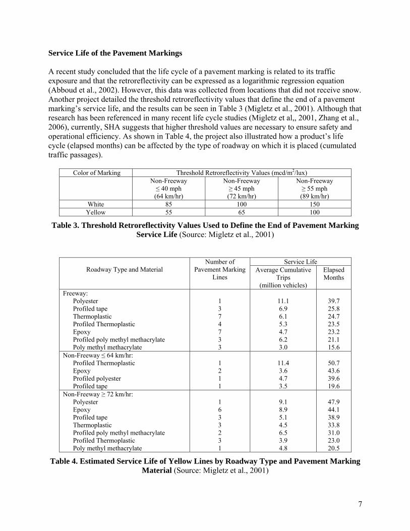
Service Life of the Pavement Markings A recent study concluded that the life cycle of a pavement marking is related to its traffic exposure and that the retroreflectivity can be expressed as a logarithmic regression equation (Abboud et al., 2002). However, this data was collected from locations that did not receive snow. Another project detailed the threshold retroreflectivity values that define the end of a pavement marking’s service life, and the results can be seen in Table 3 (Migletz et al., 2001). Although that research has been referenced in many recent life cycle studies (Migletz et al,, 2001, Zhang et al., 2006), currently, SHA suggests that higher threshold values are necessary to ensure safety and operational efficiency. As shown in Table 4, the project also illustrated how a product’s life cycle (elapsed months) can be affected by the type of roadway on which it is placed (cumulated traffic passages).

Color of Marking Threshold Retroreflectivity Values (mcd/m2/lux) Non-Freeway

≤ 40 mph (64 km/hr)

Non-Freeway ≥ 45 mph (72 km/hr)

Non-Freeway ≥ 55 mph (89 km/hr)

White 85 100 150 Yellow 55 65 100

Table 3. Threshold Retroreflectivity Values Used to Define the End of Pavement Marking Service Life (Source: Migletz et al., 2001)

Roadway Type and Material

Number of Pavement Marking

Lines

Service Life Average Cumulative

Trips (million vehicles)

Elapsed Months

Freeway: Polyester Profiled tape Thermoplastic Profiled Thermoplastic Epoxy Profiled poly methyl methacrylate Poly methyl methacrylate

1 3 7 4 7 3 3

11.1 6.9 6.1 5.3 4.7 6.2 3.0

39.7 25.8 24.7 23.5 23.2 21.1 15.6

Non-Freeway ≤ 64 km/hr: Profiled Thermoplastic Epoxy Profiled polyester Profiled tape

1 2 1 1

11.4 3.6 4.7 3.5

50.7 43.6 39.6 19.6

Non-Freeway ≥ 72 km/hr: Polyester Epoxy Profiled tape Thermoplastic Profiled poly methyl methacrylate Profiled Thermoplastic Poly methyl methacrylate

1 6 3 3 2 3 1

9.1 8.9 5.1 4.5 6.5 3.9 4.8

47.9 44.1 38.9 33.8 31.0 23.0 20.5

Table 4. Estimated Service Life of Yellow Lines by Roadway Type and Pavement Marking Material (Source: Migletz et al., 2001)

8

Phase I Results and the Difficulties in the Regression Analysis

In Phase I, the four following basic regression equations were examined to find the function that best fit the data.

• Linear : Y = a + b1 X1 + b2 X2 + b3 X3 (1) • Linear with quadratic: Y = a + b1 X1 + b2 X2 + b3 X3 + b4 (X1)2 + b5 (X2)2 + b6 (X3)2 (2) • Natural log: Ln(Y) = a + b1 Ln(X1) + b2 Ln(X2) + b3 Ln(X3) (3) • Natural log with quadratic: Ln(Y) = a + b1 Ln(X1) + b2 Ln(X2) + b3 Ln(X3)

+ b4 Ln((X1)2) + b5 Ln((X2)2) + b6 Ln((X3)2) (4)

where: Y = retroreflectivity a = intercept bi = coefficient X1 = cumulative traffic amounts (AADT/lane) X2 = cumulative precipitation X3 = cumulative snowfall

The research team expected difficulties in Phase I’s regression analysis because the brief data collection period meant that the required estimation would be outside of the data range. For the one-year period, maximum cumulative snowfall was 88 inches and the maximum cumulative traffic per lane was 3 million cars. Since the studied materials are known to last more than 3 years and possibly more than 5 years, there would be too many uncertainties in the performance forecast. Regression analysis is not good for forecasting outside of the data range (i.e., future events), but it is good for estimating events that have not actually occurred but are within the data range. In order to produce a reasonable estimation, the collected data range must be long enough to include the life cycle. Because the durable materials’ retroreflectivity did not diminish with a clear trend during the one-year data collection period, the regression analysis resulted in different scenarios for each basic function (Figure 3). The second concern was the shapes of the functions’ curves with one year of data. As shown in Figure 4, the retroreflectivity of the durable materials did not change as much in the first year as waterborne paint’s did. This characteristic made it difficult to predict the future performance of the durable materials. Additionally, retroreflectivity tends to increase in the first few months after application of the material.

9

Figure 3. Examples of the Regression Analysis with Different Basic Equations for the Durable Materials with One Year of Data

Figure 4. Typical Retroreflectivity Curves for the Different Pavement Marking Materials

2 year 1 year Time

Ret

rore

flect

ivity

3 year

Durable materials

Waterborne paint

2 year 1 year Time

Ret

rore

flect

ivity

3 year

Durable materials

10

Since the retroreflectivity levels for the durable materials were relatively high (about 300-800 mcd/m2/lux) compared to the threshold values (80-150 mcd/m2/lux) during the first year, the estimation of the life cycles was very sensitive. Figure 5 shows that the life cycle of the durable material can be very sensitive depending on the coefficients of the variables for the estimated curve. In contrast, waterborne paint’s life cycle estimation was less sensitive because its retroreflectivity values after the first year were very close to the threshold value. This characteristic means the life cycle variance can be a few years for a durable material and a few months for waterborne paint. The Phase I results were not prominent for the aforementioned reasons. None of the four regression equations were consistent for any of the conditions, establishing that the research required more data to predict the retroreflectivity of the durable materials.

Figure 5. Different Life Cycles with Different Estimation Curves

2 year 1 year Time

Ret

rore

flect

ivity

3 year

Durable materials

Waterborne paint Threshold value

11

METHODOLOGY Data Selection The three inputs used in this analysis were cumulated annual average daily traffic (AADT) per lane, cumulated precipitation, and cumulated snowfall. Many studies use total cumulated AADT, but the research team believed that cumulated AADT per lane better represented the chance of exposure to traffic. The research team focused on cumulated precipitation and cumulated snowfall because they can serve as proxy inputs for other weather-related variables. Retroreflectivity was considered the only output of the relationship, and the research team used it to calculate life cycle and economic efficiency.

Data Collection

Retroreflectivity Data Collection Methods

The SHA collected retroreflectivity data at the six locations six or seven times a year for the following marking types: white edge (WE), white skip (WS), yellow center (YC), yellow edge (YE), and yellow skip (YS). In addition to retroreflectivity, SHA recorded the number of lanes and AADT for each test site. Morgan State University collected the daily precipitation and snowfall amounts from each site’s nearest weather station. The collection schedule can be seen in Table 5. Data was collected more frequently in the winter because the previous waterborne paint study found that snow removal can be an important factor in the deterioration of a pavement marking’s retroreflectivity. As shown in Figure 6, the retroreflectivity data was measured at the exact same five points at each mile point for all five mile points at each location.

Retroreflectivity Measuring Equipment

Retroreflectivity was measured with the LTL-X retrometer (Figure 7). Produced by Delta Company in Denmark, the LTL-X retrometer is a portable field instrument that measures retroreflection in terms of RL, the coefficient of retroreflected luminance, according to international agreements. The LTL-X illuminates the road at an angle of 1.24°, and the reflected light is measured at an angle of 2.29° that corresponds to an observation distance of 100 feet (30 m). (These measurements mimic a driver’s visibility field under normal conditions.)

The instrument’s illumination field is approximately 80 inches x 18 inches (200 mm x 45 mm), and the observation field is about 244 inches x 24 inches (610 mm x 60 mm). The tower of the LTL-X contains the illumination and observation system and the control electronics. An optical system at the bottom of the tower directs a beam of light toward the road surface through a dust-protection window. A polymer shielding covers the measuring area for normal operation.

The LTL-X is controlled by multiple microprocessors, and it is operated with an extractable keyboard located at the top of the retrometer. With the push of a button, it executes the measurement and displays the result in plain text. The result is automatically transferred to the internal memory. The measurement—along with its corresponding time, date, and other information—can be printed using the built-in printer.

12

(date) Route MD 5 MD 32 MD 175 MD 216 MD 611 I-68 Date Striped 12/10/2006 06/21/2006 08/01/2006 09/18/2006 11/28/2006 06/26/2007 2006 Jun 23 Jul 28 Aug 30 4 Sep 28 13 26 Oct 10 25 Nov 15 27 Dec 6 2007 Jan 29 9 17 30 4 Feb 27 22 Mar 26 9 15 22 29 Apr May 22 7 15 18 31 Jun 19 Jul 25 19 31 Aug 15 Sep 25 7 28 Oct 31 Nov 20 1 30 Dec 12 7 19 2008 Jan Feb 11 21 15 Mar 25 25 17 Apr 15 11 15 23 May 1 Jun Jul 15 10 1 8 23 29 Aug Sep Oct 20 16 1 10 30 Nov 10 Dec 2009 Jan 15 14 Feb 6 10 Mar Apr 16 9 2 7 May 14 Jun Jul 29 16 22 14 1 Aug 3 Sept Oct 8 Nov 17 Dec 15 2010 Jan 12 7 Feb March April May 13 Jun 15 3 8 11 17

Table 5. Retroreflectivity Data Collection Schedules

13

Figure 6. Photo of Test Site with Spot Markings

Figure 7. Retroreflectivity Measuring Equipment (Delta LTL-X)

14

Data Entry

The retroreflectivity data collected by SHA was handwritten, and the data needed to be entered into an electronic file for analysis. The Morgan State University project team entered the retroreflectivity data and the weather-related information into an electronic file on a monthly basis during the data collection period.

Regression Analysis

Regression analysis is the main method for estimating the relationship between the output (retroreflectivity) and inputs in this study. It involves a single dependent variable or response, Y, which is uncontrolled. The response depends on one or more independent or regressor variables that are measured with negligible error and are controlled. The relationship fit to a set of experimental data is characterized by a prediction equation called a regression equation. It is called single variable regression if there is only one regressor or multi-variable regression if there are more than two regressors.

The smaller the variability of the residual values around the regression line relative to the overall variability, the better the prediction. For example, if there is no relationship between the x and Y variables, then the ratio of the residual variability of the Y variable to the original variance is equal to 1.0. If x and Y are perfectly related, then there is no residual variance and the ratio of variance is zero. In most cases, the ratio would fall somewhere between 0 and 1.0. One minus this ratio is referred to as R-square or the coefficient of determination. This value is immediately interpretable in the following manner. An R-square of 0.4 means that the variability of the Y values around the regression line is 1-0.4 times the original variance. In other words, 40 percent of the original variability has been explained and 60 percent residual variability remains. Ideally, most, if not all, of the original variability would be explained. The R-square value is an indicator of how well the model fits the data (i.e., an R-square close to 1.0 indicates that almost all of the variability with the variables specified in the model has been explained).

The adjusted R-square attempts to yield a more honest value to estimate the R-square for the population. The value of the R-square was .4892, and the value of the adjusted R-square was 0.4788. Adjusted R-square is computed using the formula 1 - ((1 - Rsq) ((N - 1) / (N - k - 1)). This formula shows that a small number of observations and a large number of predictors will produce a greater difference between R-square and adjusted R-square because the ratio of (N - 1) / (N - k - 1) will be much greater than one. By contrast, when the number of observations is larger than the number of predictors, the value of R-square and adjusted R-square will be much closer because the ratio of (N - 1) / (N - k - 1) will approach one.

To find the data’s correct estimation function, this project used the same four basic regression equations (Equations 1-4) examined in Phase I.

15

Analysis Process

Figure 8 summarizes the analysis process for this project.

Life Cycle Estimation for the Different Materials

The proper regression equation and the threshold values in Table 3 will estimate the life cycles of the pavement marking materials. The three input variables used to estimate retroreflectivity were all dependent on the number of days. In order to find the relationship between retroreflectivity

Regression Analysis

Economic Efficiency Evaluation

Life Cycle Estimation

Sensitivity Analysis

Data Collection

Input Variables Output (Retroreflectivity)

Threshold Values

Traffic & Weather Conditions

Installation Costs

Amount of Changes

Figure 8. Flow Chart for the Analysis

16

and number of days, the unit values for those variables were fixed as typical low, medium, and high.

The typical low, medium, and high values for daily traffic—1500 AADT per lane, 3000 AADT per lane, and 6000 AADT per lane, respectively—were based on the traffic amounts at the study locations.

The snowfall values were based on the two-year average at the study locations. The typical annual heavy snowfall amount, 88 inches per year, was based on the amounts in the western area. The central region was the basis for the moderate amount (20 inches per year), and the eastern area was the basis for the light amount (13 inches per year). The annual precipitation—30 inches per year—was similar throughout the regions. Table 6 shows the nine typical combinations of traffic and snowfall amounts for life cycle analysis in this research.

Snowfall → Traffic ↓

Light (Eastern)

Moderate (Central)

Heavy (Western)

Low 1500 AADT/lane 13 inches/year

1500 AADT/lane 22 inches/year


Medium 3000 AADT/lane 13 inches/year



High 6000 AADT/lane 13 inches/year



Annual precipitation is assumed to be 30 inches per year for all nine combinations.

Table 6. Typical Combinations for Life Cycle Analysis

Cost Estimation for the Different Materials In order to estimate economic efficiency, the research team had to calculate the costs to install each product in terms of money, delay, and potential accidents.

The research team based monetary installation costs on the state of Maryland’s application bills from construction companies. In general, the unit cost depended on the total length of the pavement marking applications. Therefore, the best way to estimate the monetary installation costs was to find the regression equation that showed the relationship between the unit cost and the project’s installation length.

However, in this research, the unit installation costs were estimated as the average unit costs of the major application projects as shown in Tables 7-10. This was done to minimize the complexity of trying to estimate the installation costs for different project lengths.

Tables 7-9 show the average unit costs for a five-inch-wide piece of inlaid tape, thermoplastic, and waterborne paint from various pavement marking projects. Table 10 compares the unit costs of the three pavement marking materials.

17

Location Length of Marking (ft) Total Cost ($) Unit Cost ($/ft) MD 32 5,982 27,517.2 4.60 MD 175 3,971 11,913.0 3.00 MD 216 13,359 40,077.0 3.00 US 301 18,066 56,004.6 3.10 US 219 10,560 29,040.0 2.75

Total / Average 51,938 164,551.8 3.168

Table 7. Unit Cost Estimation for Inlaid Tape

Location Length of Marking (ft) Total Costs ($) Unit Cost ($/ft) MD 32 32,942 27,517.2 0.42 MD 216 13,210 5,284.0 0.40

US 1 6,479 4,859.63 0.75 MD 940 6,727 4,036.2 0.60 US 40 6,944.32 8,680.4 1.25

Total / Average 66302.32 50,377.43 0.760

Table 8. Unit Cost Estimation for Thermoplastic

Location Length of Marking (ft) Total Costs ($) Unit Cost ($/ft) MD 135 72,963 10,214.82 0.14 MD 295 24,144 3,757.92 0.16

Total / Average 97,107 13,972.74 0.144

Table 9. Unit Cost Estimation for Waterborne Paint

Material Installation Costs ($/ft) Waterborne Paint 0.144 Thermoplastic 0.760 Inlaid Tape 3.168

Table 10. Installation Costs for the Different Pavement Marking Materials in Maryland

A pavement marking’s installation usually causes traffic delays because the installation vehicle is slow and lanes are sometimes blocked. Because each of the materials examined in this research had a different installation process, the research team estimated the delay costs for each product under different conditions.

The basic input variables for estimating delay were the number of lanes, the traffic amount, and the road length of the project. The research team also had to assume the installation vehicle’s speed. With those input variables, the delays were estimated through VISSUM, the traffic simulation software. Then, regression analysis was performed to find the relationship between the delay and input variables, so delay can be estimated when the input variables are available. Thus, information about the installation site allows estimation of the installation-caused delay.

18

Although the research team developed a process to find the delay for specific conditions, this study used one average delay cost in order to simplify the cost estimation. However, if site-specific delay estimation is necessary, it can be found using the regression equation for the site’s specific conditions.

The general delay cost was based on a two-lane, half-mile road section with a traffic volume of 1,000 vehicles per hour. Inlaid tape required no additional delay because the material is applied during the paving process.

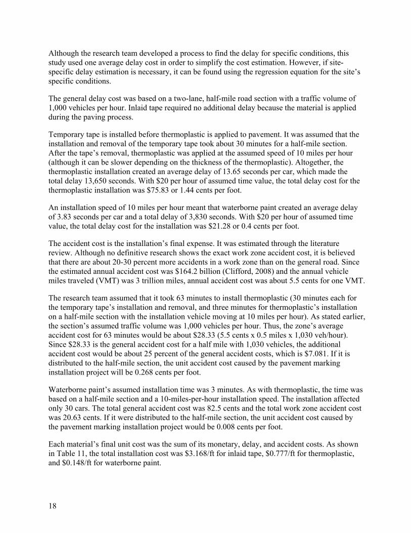
Temporary tape is installed before thermoplastic is applied to pavement. It was assumed that the installation and removal of the temporary tape took about 30 minutes for a half-mile section. After the tape’s removal, thermoplastic was applied at the assumed speed of 10 miles per hour (although it can be slower depending on the thickness of the thermoplastic). Altogether, the thermoplastic installation created an average delay of 13.65 seconds per car, which made the total delay 13,650 seconds. With $20 per hour of assumed time value, the total delay cost for the thermoplastic installation was $75.83 or 1.44 cents per foot.

An installation speed of 10 miles per hour meant that waterborne paint created an average delay of 3.83 seconds per car and a total delay of 3,830 seconds. With $20 per hour of assumed time value, the total delay cost for the installation was $21.28 or 0.4 cents per foot.

The accident cost is the installation’s final expense. It was estimated through the literature review. Although no definitive research shows the exact work zone accident cost, it is believed that there are about 20-30 percent more accidents in a work zone than on the general road. Since the estimated annual accident cost was $164.2 billion (Clifford, 2008) and the annual vehicle miles traveled (VMT) was 3 trillion miles, annual accident cost was about 5.5 cents for one VMT.

The research team assumed that it took 63 minutes to install thermoplastic (30 minutes each for the temporary tape’s installation and removal, and three minutes for thermoplastic’s installation on a half-mile section with the installation vehicle moving at 10 miles per hour). As stated earlier, the section’s assumed traffic volume was 1,000 vehicles per hour. Thus, the zone’s average accident cost for 63 minutes would be about $28.33 (5.5 cents x 0.5 miles x 1,030 veh/hour). Since $28.33 is the general accident cost for a half mile with 1,030 vehicles, the additional accident cost would be about 25 percent of the general accident costs, which is $7.081. If it is distributed to the half-mile section, the unit accident cost caused by the pavement marking installation project will be 0.268 cents per foot.

Waterborne paint’s assumed installation time was 3 minutes. As with thermoplastic, the time was based on a half-mile section and a 10-miles-per-hour installation speed. The installation affected only 30 cars. The total general accident cost was 82.5 cents and the total work zone accident cost was 20.63 cents. If it were distributed to the half-mile section, the unit accident cost caused by the pavement marking installation project would be 0.008 cents per foot.

Each material’s final unit cost was the sum of its monetary, delay, and accident costs. As shown in Table 11, the total installation cost was $3.168/ft for inlaid tape, $0.777/ft for thermoplastic, and $0.148/ft for waterborne paint.

19

Inlaid Tape ($/ft) Thermoplastic ($/ft) Waterborne Paint ($/ft) Installation cost 3.168 0.760 0.144

Delay cost - 0.0144 0.004 Accident cost - 0.00268 0.00008

Total installation cost 3.168 0.777 0.148

Table 11. Summary of Total Installation Cost Estimation

Economic Efficiency Estimation for the Different Materials

Because installation costs occur once in a material’s life cycle, the costs were distributed throughout the life cycle. As shown in Equation 5, this was done by converting present value to annual value with an assumed interest rate (or simply it can be divided by the life cycle, assuming that there is no interest for distributing the installation costs through the life cycle). The pavement marking material with the lowest annual cost is the most economically efficient material.

n

n

iii

PVA

)1(1)1(

+−+

= (5)

where: A = annual costs (or monthly costs) PV = present value of installation costs i = interest rate (per year or per month) n = life cycle (number of years or months)

20

21

RESEARCH FINDINGS This research estimated the performance and life cycle of inlaid tape and thermoplastic based on three to four years of data collection. Since the data collection period was long enough, retroreflectivity values at certain locations became close to the threshold values and the resulting regression analysis was more reasonable. Regression Analysis Tables 12-15 show the regression results for inlaid tape and thermoplastic. The three variables used in the regression analysis were precipitation, snowfall, and traffic amount. As shown in the tables, because the linear function had the highest R-square value of all the equations, it best fit all four materials (white inlaid tape, yellow inlaid tape, white thermoplastic, and yellow thermoplastic). White inlaid tape’s adjusted R-square values indicate the correctness of the estimation. Not only were white inlaid tape’s adjusted R-square values higher than the values of the other materials studied in this project, but they were also higher than the values in other research. However, yellow thermoplastic’s R-square value was extremely low, which may indicate that the regression analysis produced imprecise retroreflectivity estimates. The field data caused most of the inconsistency in the data and the regression analysis.

The retroreflectivity curves in Figures 9-26 were based on the nine traffic and snowfall combinations in Table 6. Figures 9-17 show the estimated retroreflectivity curves of white inlaid tape and thermoplastic. The curves had a similar shape and were almost parallel in all nine cases, showing that both materials’ basic depreciation characteristics were very similar. The only major difference was the materials’ initial retroreflectivity values.

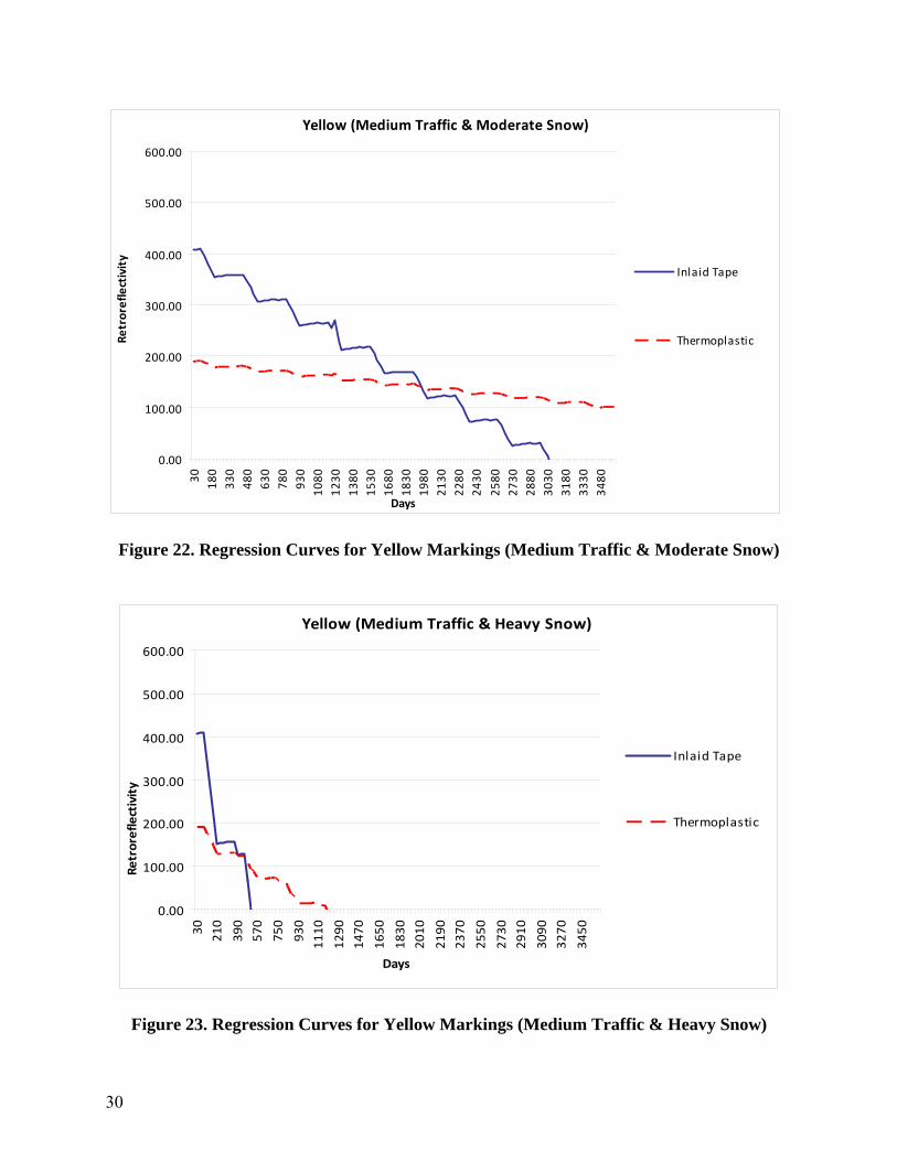
Figures 18-26 show the estimated retroreflectivity curves of yellow inlaid tape and thermoplastic. Unlike the white pavement markings, the shapes of both curves were different. Although yellow inlaid tape had a higher initial retroreflectivity, it deteriorated faster than yellow thermoplastic. After a certain period, yellow thermoplastic’s retroreflectivity was higher that yellow inlaid tape’s.

The estimates for the yellow markings were not as good as the estimates for the white markings. As shown in the regression tables, the yellow markings’ adjusted R-square values were low. In particular, yellow thermoplastic’s R-square value was very low. The estimation of the retroreflectivity values may not be correct and reasonable. The yellow markings’ low R-square values will be explained in the validation section.

Figures 9-26 show that the retroreflectivity curves were more sensitive to snowfall than traffic amounts (i.e., the snowfall amount, not traffic, was the major factor in retroreflectivity’s deterioration). This will be discussed further in the life cycle analysis.

22

Linear Log Nonlinear Nonlinear Log Number of Observations 7603 7603 7603 7603 F-Value 2433.4 1113.27 - - Adjusted R-square 0.5015 0.31722 0.334 0.334 Intercept 762.81 6.4379 755.2 6.51 Coef. for cumulative traffic -1E^-05 0.051837 0.000016 -129.92 Coef. for cumulative traffic square - - 1.78X10-12 64.98 Coef. for cumulative precipitation -0.41259 -0.16495 -860 502.76 Coef. for cumulative precipitation sq. - - 0.00042 -251.45 Coef. for cumulative snow -0.98892 -0.07279 -.795 -511.76 Coef. for cumulative snow square - - 0.00054 255.83

Table 12. Regression Results for White Inlaid Tape

Linear Log Nonlinear Nonlinear Log Number of Observations 3121 3121 3121 3121 F-Value 623.438 411.4319 - - Adjusted R-square 0.388 0.2948 0.301 0.30089 Intercept 405.66 4.45 434.1 4.36 Coef. for cumulative traffic 4.5E^-6 .1286 .000019 129.18 Coef. for cumulative traffic square - - -7.5X10-13 -64.52 Coef. for cumulative precipitation .231 -.02015 -.023 142.4 Coef. for cumulative precipitation sq. - - .00033 -71.21 Coef. for cumulative snow -2.938 -.184 -4.58 -781.21 Coef. for cumulative snow square - - .0068 390.51

Table 13. Regression Results for Yellow Inlaid Tape

Linear Log Nonlinear Nonlinear Log Number of Observations 7816 7816 7816 7816 F-Value 794.419 793.92 - - Adjusted R-square 0.2748 0.2747 0.140 0.140 Intercept 348.91 11.15 341.7 12.09 Coef. for cumulative traffic -9.4E^-6 -.477 -.000035 201.26 Coef. for cumulative traffic square - - 1.21X10-12 -100.89 Coef. for cumulative precipitation .0688 .3395 .804 -.636 Coef. for cumulative precipitation sq. - - -.0004 .439 Coef. for cumulative snow -1.3577 -0.1066 -3.401 589.30 Coef. for cumulative snow square - - .0078 -294.64

Table 14. Regression Results for White Thermoplastic

23

Linear Log Nonlinear Nonlinear Log Number of Observations 4664 4664 4664 4664 F-Value 172.1843 100.3737 - - Adjusted R-square 0.1129 0.0688 0.001 0.00141 Intercept 189.57 4.545 154.7 4.698 Coef. for cumulative traffic 4.96E^-6 0.0453 0.000013 105.23 Coef. for cumulative traffic square - - -8.02X10-13 -52.60 Coef. for cumulative precipitation .0115 -.0214 .1274 1230.84 Coef. for cumulative precipitation sq. - - 0.000037 -615.42 Coef. for cumulative snow -0.7233 -0.084 -.7372 40.60 Coef. for cumulative snow square - - -.00248 -20.30

Table 15. Regression Results for Yellow Thermoplastic

Figure 9. Regression Curves for White Markings (Low Traffic & Light Snow)

White (Low Traffic & Light Snow)

0.00

200.00

400.00

600.00

800.00

1000.00

1200.00

30 180

330

480

630

780

930

1080

1230

1380

1530

1680

1830

1980

2130

2280

2430

2580

2730

2880

3030

3180

3330

3480

Days

Ret

rore

flect

ivity

Inlaid Tape

Thermoplastic

24

Figure 10. Regression Curves for White Markings (Low Traffic & Moderate Snow)

Figure 11. Regression Curves for White Markings (Low Traffic & Heavy Snow)

White (Low Traffic & Moderate Snow)

0.00

200.00

400.00

600.00

800.00

1000.00

1200.00

30 180

330

480

630

780

930

1080

1230

1380

1530

1680

1830

1980

2130

2280

2430

2580

2730

2880

3030

3180

3330

3480

Days

Ret

rore

flect

ivity

Inlaid Tape

Thermoplastic

White (Low Traffic & Heavy Snow)

0.00

200.00

400.00

600.00

800.00

1000.00

1200.00

30 180

330

480

630

780

930

1080

1230

1380

1530

1680

1830

1980

2130

2280

2430

2580

2730

2880

3030

3180

3330

3480

Days

Ret

rore

flect

ivity

Inlaid Tape

Thermoplastic

25

Figure 12. Regression Curves for White Markings (Medium Traffic & Light Snow)

Figure 13. Regression Curves for White Markings (Medium Traffic & Moderate Snow)

White (Medium Traffic and Light Snow)

0.00

200.00

400.00

600.00

800.00

1000.00

1200.00

30 180

330

480

630

780

930

1080

1230

1380

1530

1680

1830

1980

2130

2280

2430

2580

2730

2880

3030

3180

3330

3480

Days

Retroreflectivity

Inlaid Tape

Thermoplastic

White (Medium Traffic & Moderate Snow)

0.00

200.00

400.00

600.00

800.00

1000.00

1200.00

30 180

330

480

630

780

930

1080

1230

1380

1530

1680

1830

1980

2130

2280

2430

2580

2730

2880

3030

3180

3330

3480

Days

Retroreflectivity

Inlaid Tape

Thermoplastic

26

Figure 14. Regression Curves for White Markings (Medium Traffic & Heavy Snow)

Figure 15. Regression Curves for White Markings (High Traffic & Light Snow)

White (Medium Traffic & Heavy Snow)

0.00

200.00

400.00

600.00

800.00

1000.00

1200.00

30 210

390

570

750

930

1110

1290

1470

1650

1830

2010

2190

2370

2550

2730

2910

3090

3270

3450

Days

Retroreflectivity

Inlaid Tape

Thermoplastic

White (High Traffic & Light Snow)

0.00

200.00

400.00

600.00

800.00

1000.00

1200.00

30 180

330

480

630

780

930

1080

1230

1380

1530

1680

1830

1980

2130

2280

2430

2580

2730

2880

3030

3180

3330

3480

Days

Ret

rore

flect

ivity

Inlaid Tape

Thermoplastic

27

Figure 16. Regression Curves for White Markings (High Traffic & Moderate Snow)

Figure 17. Regression Curves for White Markings (High Traffic & Heavy Snow)

White (High Traffic & Moderate Snow)

0.00

200.00

400.00

600.00

800.00

1000.00

1200.00

30 180

330

480

630

780

930

1080

1230

1380

1530

1680

1830

1980

2130

2280

2430

2580

2730

2880

3030

3180

3330

3480

Days

Ret

rore

flect

ivity

Inlaid Tape

Thermoplastic

White (High Traffic & Heavy Snow)

0.00

200.00

400.00

600.00

800.00

1000.00

1200.00

30 180

330

480

630

780

930

1080

1230

1380

1530

1680

1830

1980

2130

2280

2430

2580

2730

2880

3030

3180

3330

3480

Days

Ret

rore

flect

ivity

Inlaid Tape

Thermoplastic

28

Figure 18. Regression Curves for Yellow Markings (Low Traffic & Light Snow)

Figure 19. Regression Curves for Yellow Markings (Low Traffic & Moderate Snow)

Yellow (Low Traffic & Light Snow)

0.00

100.00

200.00

300.00

400.00

500.00

600.00

30 210

390

570

750

930

1110

1290

1470

1650

1830

2010

2190

2370

2550

2730

2910

3090

3270

3450

Days

Ret

rore

flect

ivity

Inlaid Tape

Thermoplastic

Yellow (Low Traffic & Moderate Snow)

0.00

100.00

200.00

300.00

400.00

500.00

600.00

30 180

330

480

630

780

930

1080

1230

1380

1530

1680

1830

1980

2130

2280

2430

2580

2730

2880

3030

3180

3330

3480

Days

Ret

rore

flect

ivity

Inlaid Tape

Thermoplastic

29

Figure 20. Regression Curves for Yellow Markings (Low Traffic & Heavy Snow)

Figure 21. Regression Curves for Yellow Markings (Medium Traffic & Light Snow)

Yellow (Low Traffic & Heavy Snow)

0.00

100.00

200.00

300.00

400.00

500.00

600.00

30 180

330

480

630

780

930

1080

1230

1380

1530

1680

1830

1980

2130

2280

2430

2580

2730

2880

3030

3180

3330

3480

Days

Ret

rore

flect

ivity Inlaid Tape

Thermoplastic

Yellow (Medium Traffic & Light Snow)

0.00

100.00

200.00

300.00

400.00

500.00

600.00

30 210

390

570

750

930

1110

1290

1470

1650

1830

2010

2190

2370

2550

2730

2910

3090

3270

3450

Days

Ret

rore

flect

ivity

Inlaid Tape

Thermoplastic

30

Figure 22. Regression Curves for Yellow Markings (Medium Traffic & Moderate Snow)

Figure 23. Regression Curves for Yellow Markings (Medium Traffic & Heavy Snow)

Yellow (Medium Traffic & Moderate Snow)

0.00

100.00

200.00

300.00

400.00

500.00

600.00

30 180

330

480

630

780

930

1080

1230

1380

1530

1680

1830

1980

2130

2280

2430

2580

2730

2880

3030

3180

3330

3480

Days

Retroreflectivity

Inlaid Tape

Thermoplastic

Yellow (Medium Traffic & Heavy Snow)

0.00

100.00

200.00

300.00

400.00

500.00

600.00

30 210

390

570

750

930

1110

1290

1470

1650

1830

2010

2190

2370

2550

2730

2910

3090

3270

3450

Days

Retroreflectivity

Inlaid Tape

Thermoplastic

31

Figure 24. Regression Curves for Yellow Markings (High Traffic & Light Snow)

Figure 25. Regression Curves for Yellow Markings (High Traffic & Moderate Snow)

Yellow (High Traffic & Light Snow)

0.00

100.00

200.00

300.00

400.00

500.00

600.00

30 150

270

390

510

630

750

870

990

1110

1230

1350

1470

1590

1710

1830

1950

2070

2190

2310

2430

2550

2670

2790

2910

3030

3150

3270

3390

3510

Days

Ret

rore

flect

ivity

Inlaid Tape

Thermoplastic

Yellow (High Traffic & Moderate Snow)

0.00

100.00

200.00

300.00

400.00

500.00

600.00

30 180

330

480

630

780

930

1080

1230

1380

1530

1680

1830

1980

2130

2280

2430

2580

2730

2880

3030

3180

3330

3480

Days

Ret

rore

flect

ivty

Inlaid

Thermoplastic

32

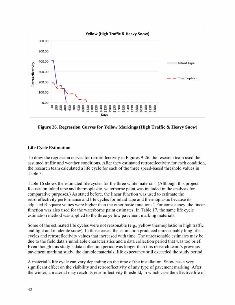
Figure 26. Regression Curves for Yellow Markings (High Traffic & Heavy Snow)

Life Cycle Estimation

To draw the regression curves for retroreflectivity in Figures 9-26, the research team used the assumed traffic and weather conditions. After they estimated retroreflectivity for each condition, the research team calculated a life cycle for each of the three speed-based threshold values in Table 3.

Table 16 shows the estimated life cycles for the three white materials. (Although this project focuses on inlaid tape and thermoplastic, waterborne paint was included in the analysis for comparative purposes.) As stated before, the linear function was used to estimate the retroreflectivity performance and life cycles for inlaid tape and thermoplastic because its adjusted R-square values were higher than the other basic functions’. For consistency, the linear function was also used for the waterborne paint estimates. In Table 17, the same life cycle estimation method was applied to the three yellow pavement marking materials.

Some of the estimated life cycles were not reasonable (e.g., yellow thermoplastic in high traffic and light and moderate snow). In those cases, the estimation produced unreasonably long life cycles and retroreflectivity values that increased with time. The unreasonable estimates may be due to the field data’s unreliable characteristics and a data collection period that was too brief. Even though this study’s data collection period was longer than this research team’s previous pavement marking study, the durable materials’ life expectancy still exceeded the study period.

A material’s life cycle can vary depending on the time of the installation. Snow has a very significant effect on the visibility and retroreflectivity of any type of pavement marking. After the winter, a material may reach its retroreflectivity threshold, in which case the effective life of

Yellow (High Traffic & Heavy Snow)

0.00

100.00

200.00

300.00

400.00

500.00

600.00

30 180

330

480

630

780

930

1080

1230

1380

1530

1680

1830

1980

2130

2280

2430

2580

2730

2880

3030

3180

3330

3480

Days

Ret

rore

flect

ivity Inlaid Tape

Thermoplastic

33

the pavement marking ends. For this project, the life cycle estimates were based on a September installation of the materials. Of course, installations during a different time of the year would yield different life cycle estimates.

Condition Inlaid Tape Thermoplastic Waterborne Paint

Low Traffic & Light Snow 240, 258, 264 113, 144, 156 9, 18, 19 Low Traffic & Moderate Snow 201, 218, 223 78, 100, 103 6, 16,16

Low Traffic & Heavy Snow 67, 76, 77 18, 25, 28 3, 4, 4 Medium Traffic & Light Snow 221, 239, 243 91, 114, 126 15, 18, 18

Medium Traffic & Moderate Snow 173, 188, 193 65, 85, 89 6, 16, 17 Medium Traffic & Heavy Snow 64, 72, 73 16, 18, 24 3, 4, 4

High Traffic & Light Snow 157, 172, 176 65, 82, 88 15, 18, 19 High Traffic & Moderate Snow 137, 149, 152 65, 78, 89 6, 16, 17

High Traffic & Heavy Snow 60, 64, 65 16, 18, 19 3, 4, 4

Units represent number of months. Life cycles are based on thresholds of 150, 100, and 85 mcd/m2/lux, respectively.

Table 16. Estimated Life Cycle of White Pavement Marking Materials Condition Inlaid Tape Thermoplastic Waterborne

Paint Low Traffic & Light Snow 127, 142, 146 170, 242, 262 6, 13, 14

Low Traffic & Moderate Snow 76, 79, 80 66, 90, 100 12, 13, 13 Low Traffic & Heavy Snow 18, 18, 19 7, 18, 18 4, 4, 4

Medium Traffic & Light Snow 140, 157, 162 270, 275, 299 12, 13, 13 Medium Traffic & Moderate Snow 76, 88, 88 114, 156, 167 12, 13, 13

Medium Traffic & Heavy Snow 15, 16, 16 16, 21, 21 4, 4, 4 High Traffic & Light Snow 174, 195, 201 - 12, 13, 13

High Traffic & Moderate Snow 88, 90, 100 - 12, 13, 13 High Traffic & Heavy Snow 15, 16, 16 17, 27, 28 4, 4, 4

Units represent number of months. Life cycles are based on thresholds of 100, 65, and 55 mcd/m2/lux, respectively.

Table 17. Estimated Life Cycle of Yellow Pavement Marking Materials

Validation of the Regression Analysis and Life Cycle Estimation

The regression analysis produced the estimated life cycles (Tables 16 and 17). In order to validate the estimation, the regression results were compared to the actual collected data.

Inlaid tape showed rather consistent results. The white inlaid tape on MD 611, which is in the eastern area of the state and receives little snow, had the highest average retroreflectivity. At the same time, the white inlaid tape on I-68, which is in the western area of the state and receives the heaviest snowfalls, had the lowest average retroreflectivity.

For the heavy snow and high traffic conditions, white inlaid tape’s estimated life cycle was five years and yellow inlaid tape’s estimated life cycle was two years. The real data for I-68 shows that the white markings’ average retroreflectivity is 166 and the yellow markings’ average

34

retroreflectivity after three years is 73. The real data confirmed the regression analysis and life cycle estimation for inlaid tape.

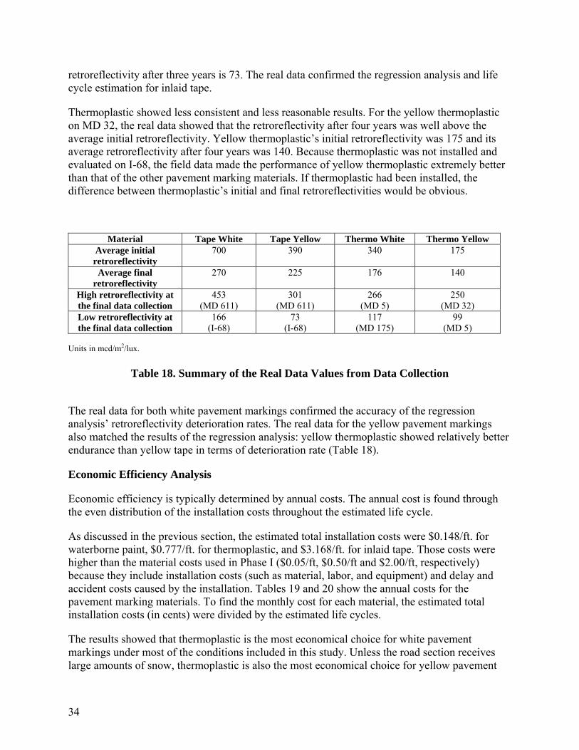
Thermoplastic showed less consistent and less reasonable results. For the yellow thermoplastic on MD 32, the real data showed that the retroreflectivity after four years was well above the average initial retroreflectivity. Yellow thermoplastic’s initial retroreflectivity was 175 and its average retroreflectivity after four years was 140. Because thermoplastic was not installed and evaluated on I-68, the field data made the performance of yellow thermoplastic extremely better than that of the other pavement marking materials. If thermoplastic had been installed, the difference between thermoplastic’s initial and final retroreflectivities would be obvious.

Material Tape White Tape Yellow Thermo White Thermo YellowAverage initial retroreflectivity

700 390 340 175

Average final retroreflectivity

270 225 176 140

High retroreflectivity at the final data collection

453 (MD 611)

301 (MD 611)

266 (MD 5)

250 (MD 32)

Low retroreflectivity at the final data collection

166 (I-68)

73 (I-68)

117 (MD 175)

99 (MD 5)

Units in mcd/m2/lux.

Table 18. Summary of the Real Data Values from Data Collection

The real data for both white pavement markings confirmed the accuracy of the regression analysis’ retroreflectivity deterioration rates. The real data for the yellow pavement markings also matched the results of the regression analysis: yellow thermoplastic showed relatively better endurance than yellow tape in terms of deterioration rate (Table 18).

Economic Efficiency Analysis

Economic efficiency is typically determined by annual costs. The annual cost is found through the even distribution of the installation costs throughout the estimated life cycle.

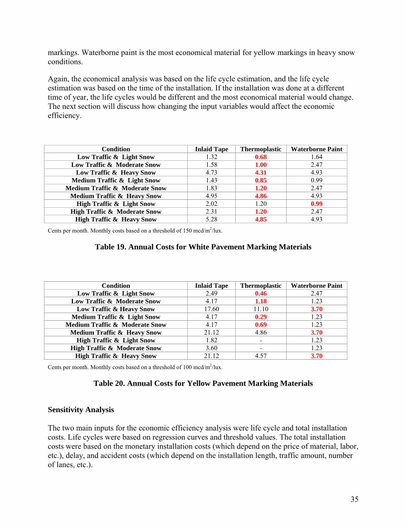
As discussed in the previous section, the estimated total installation costs were $0.148/ft. for waterborne paint, $0.777/ft. for thermoplastic, and $3.168/ft. for inlaid tape. Those costs were higher than the material costs used in Phase I ($0.05/ft, $0.50/ft and $2.00/ft, respectively) because they include installation costs (such as material, labor, and equipment) and delay and accident costs caused by the installation. Tables 19 and 20 show the annual costs for the pavement marking materials. To find the monthly cost for each material, the estimated total installation costs (in cents) were divided by the estimated life cycles.

The results showed that thermoplastic is the most economical choice for white pavement markings under most of the conditions included in this study. Unless the road section receives large amounts of snow, thermoplastic is also the most economical choice for yellow pavement

35

markings. Waterborne paint is the most economical material for yellow markings in heavy snow conditions.

Again, the economical analysis was based on the life cycle estimation, and the life cycle estimation was based on the time of the installation. If the installation was done at a different time of year, the life cycles would be different and the most economical material would change. The next section will discuss how changing the input variables would affect the economic efficiency.

Condition Inlaid Tape Thermoplastic Waterborne Paint Low Traffic & Light Snow 1.32 0.68 1.64

Low Traffic & Moderate Snow 1.58 1.00 2.47 Low Traffic & Heavy Snow 4.73 4.31 4.93

Medium Traffic & Light Snow 1.43 0.85 0.99 Medium Traffic & Moderate Snow 1.83 1.20 2.47

Medium Traffic & Heavy Snow 4.95 4.86 4.93 High Traffic & Light Snow 2.02 1.20 0.99

High Traffic & Moderate Snow 2.31 1.20 2.47 High Traffic & Heavy Snow 5.28 4.85 4.93

Cents per month. Monthly costs based on a threshold of 150 mcd/m2/lux.

Table 19. Annual Costs for White Pavement Marking Materials




Medium Traffic & Heavy Snow 21.12 4.86 3.70 High Traffic & Light Snow 1.82 - 1.23

High Traffic & Moderate Snow 3.60 - 1.23 High Traffic & Heavy Snow 21.12 4.57 3.70

Cents per month. Monthly costs based on a threshold of 100 mcd/m2/lux.

Table 20. Annual Costs for Yellow Pavement Marking Materials

Sensitivity Analysis The two main inputs for the economic efficiency analysis were life cycle and total installation costs. Life cycles were based on regression curves and threshold values. The total installation costs were based on the monetary installation costs (which depend on the price of material, labor, etc.), delay, and accident costs (which depend on the installation length, traffic amount, number of lanes, etc.).

36

The analysis would be very complicated if all those variables were included. Therefore, the sensitivity analysis in this research considered the final inputs, life cycle, and total installation costs. The lower level variables (such as threshold values, monetary installation costs, etc.) can be determined once life cycle and total installation costs are assumed. In order to be competitive to thermoplastic, inlaid tape must have either a longer life cycle or lower installation costs. Table 21 shows what happened when inlaid tape’s life cycle was increased by 50 percent. For the white markings, the increase made inlaid tape competitive to thermoplastic and more economical in high snow conditions. In this case, inlaid tape became more economical than waterborne paint in most scenarios.






Cents per month. Monthly costs are based on a threshold of 150 mcd/m2/lux.

Table 21. Annual Costs for White Pavement Marking Materials When Inlaid Tape’s Life Cycle is 50% Longer

Table 22 shows how the annual costs change when inlaid tape’s cost is 40 percent lower ($1.900 instead of $3.168). For the white pavement markings, the decrease made inlaid tape economically competitive to thermoplastic. In heavy snow conditions, regardless of the traffic amount, inlaid tape was more economical. In moderate snow areas, inlaid tape and thermoplastic were almost the same in terms of economic efficiency. In light snow areas, thermoplastic remained more economical than inlaid tape. The sensitivity analysis showed that to make the inlaid tape economically competitive, inlaid tape’s life cycle should be increased by 50 percent or its total installation costs should be decreased by 40 percent. However, inlaid tape can be more competitive to thermoplastic in heavy snow areas even with less than 50 percent increased life cycle or less than 40 percent decreased total installation cost, because inlaid tape’s relative performance to thermoplastic’s in heavy snow area is better than that in less snow areas.

37






Cents per month. Monthly costs are based on a threshold of 150 mcd/m2/lux.

Table 22. Annual Costs for White Pavement Marking Materials When Inlaid Tape’s Installation Costs are 40% Lower

38

39

CONCLUSIONS Because inlaid tape and thermoplastic are known to last more than three years—in some locations, thermoplastic lasts more than five years and inlaid tape more than eight years—the data collection period for this research was not long enough to justify various basic functions. With the data collection period for this research, the linear function was found to fit the relationship between the collected retroreflectivity data and the input variables.

Because of the inconsistent nature of the field data, the adjusted R-square values, which indicate how well the data fits the estimated function, were not very high. However, the R-square values were higher than the values found in similar research because of the inclusion of weather data and traffic data. Traffic data was the sole conventional variable for the previous life cycle studies of the pavement markings.

Snowfall amounts affected retroreflectivity more than traffic amounts did. This indicates that snowplow use must be well controlled and standardized in order to improve the pavement markings’ performance and life cycles. Increased use of rubber blades on the plows may minimize the damage to the pavement markings.

The regression results fit the real data for the white pavement markings, but they did not fit as well for the yellow pavement markings. The regression results also showed that the regression estimates of inlaid tape fit the real data better than that of thermoplastic. These results would seem to indicate that the white markings’ and inlaid tape’s performance were more stable than the yellow markings’ and thermoplastic’s. It also means that there were uncertainties in yellow pavement markings’ and thermoplastic’s performance.

The life cycles for the pavement markings were determined with the estimated retroreflectivity and threshold values. The retroreflectivity estimates were based on nine weather and traffic combinations (which were based on three snowfall amounts and three traffic amounts).

A material’s life cycle can vary greatly depending on the time of year of the installation. Snow removal has a significant effect on retroreflectivity. After a severe winter, a material typically hits its retroreflectivity threshold and the life of the pavement marking ends. For this project, the life cycle estimates were based on a September installation of the materials. Installations during a different time of the year would yield much different life cycle estimates, and, consequently, different economic efficiencies. In general, inlaid tape lasts longer than thermoplastic because inlaid tape’s initial retroreflectivity is higher than thermoplastic’s. In addition, the white pavement markings last longer than yellow pavement markings because the white pavement markings’ initial retroreflectivity is higher than the yellow pavement markings’. However, in this study, the performance of yellow thermoplastic was abnormally good. In fact, yellow thermoplastic lasted as long as white thermoplastic and yellow inlaid tape.

Estimated life cycles and total installation costs were used to determine the materials’ annual costs (i.e., economic efficiency). The estimated total installation costs were $3.168 per foot for

40

inlaid tape, $0.777 per foot for thermoplastic, and $0.148 per foot for waterborne paint. Although inlaid tape can last longer effectively, thermoplastic was more economical under most conditions because of inlaid tape’s higher installation costs. To make inlaid tape competitive to thermoplastic in terms of economic efficiency, the sensitivity analysis showed that inlaid tape’s life cycle had to be increased by 50 percent or its total installation costs had to be reduced by 40 percent. For example, inlaid tape’s life cycle would improve if the tape were set deeper in heavy snows areas—either by installing it at a higher asphalt temperature, or by cutting a groove in the pavement so that the tape was slightly below surface. Full-compliment tape projects or longer distance projects could also reduce the installation costs.

This project’s two research assistants are currently expanding upon these findings for their theses. One research is about the estimation of total installation costs, and the other examines the life cycle differences among different marking types (such as edge line, skip line, and center line). Once completed, both studies will provide better and more complete information about the life cycles of pavement marking materials.

41

REFERENCES Abboud, N., and Nowman, B. Cost- and Longevity-Based Scheduling of Paint and Thermoplastic Striping. Transportation Research Record 1794. Transportation Research Board, National Research Council, Washington, D.C., 2002, 55-62. Clifford, Catherine. U.S. Car Accident Cost: $164.2 Billion, CNNMoney.com, March 5, 2008. Jiang, X., and Adeli, H. Freeway Work Zone Traffic Delay and Cost Optimization Model, Journal of Transportation Engineering, Vol. 129, No. 3, May 2003. Jin, T., Saitoa, M., and Eggett, D. Statistical comparisons of the crash characteristics on highways between construction time and non-construction time, Accident Analysis & Prevention, Volume 40, Issue 6, November 2008. Kopf, J. Reflectivity of Pavement Markings: Analysis of Retroreflectivity Degradation Curves, Washington State Transportation Center, WA-RD 592.1, September 2004 Lee, Y., Randal, R., and Karri, G. Retroreflectivity and Life Cycle Study of Waterborne Paint Pavement Markings: Case Study for the State of Maryland. Transportation Research Board Annual Meeting, Transportation Research Board, Washington D.C., 2008. Lee, Y. Durability Study: Waterborne Paint Pavement Markings. Maryland State Highway Administration, December 2007. Lee, Y. Life Cycle and Economic Efficiency Analysis: Durable Pavement Markings, Maryland State Highway Administration, July 2009. Migletz, J., Graham, J., Bauer, K., and D. Harwood. Service Life of Durable Pavement Markings. Paper 010-447. Transportation Research Board 80th Annual Meeting Preprint CD-ROM. Transportation Research Board, National Research Council, Washington, D.C., January 2001. Migletz, J., Graham, J., Bauer, K., and D. Harwood. Field Surveys of Pavement Marking Retroreflectivity. Transportation Research Record 1657. Transportation Research Board, National Research Council, Washington, D.C., 1999, 71-78. Mohan, S., and Gautam, P. Cost of Highway Work Zone Injuries, Practice Periodical on Structural Design and Construction, Vol. 7, No. 2, May 1, 2002. Mokkapati, Naveen. Determining the Extent and Characteristics of Overrepresentation on Large Truck Crashes in Daytime and Nighttime Work Zones, MS Thesis, Texas A&M University, December 2007.

42

Montebello, D., and Schroeder, J. Cost of Pavement Marking Materials. Minnesota Local Road Research Board, March 2000. National Partnership for Highway Quality, Work Zone Fatalities, Web documents. Pavement Markings Study Nears Completion. Better Roads, Vol. 66, No. 4. April 1996. Potts, I., Harwood, D., Bokenroger, C., and Hutton, J. Benefit-Cost Evaluation of MoDOT’s Total Striping and Delineation Program, OR09.014, Midwest Research Institute and Missouri Department of Transportation, November 2008. Wang, J., Hughes, W., Council, F., and Paniati, J. Investigation of Highway Work Zone Crashes, Federal Highway Administration, FHWA-RD-96-100, 1996. Zhang, Y., and Wu, D. Methodologies to Predict Service Lives of Pavement Marking Materials Journal of the Transportation Research Forum, Vol. 45, No. 3, 2006.

Documents

Life-Cycle and Economic Efficiency Analysis - Phase II