S1

Life Cycle Carbon Footprint of Shale Gas: Review of Evidence

and Implications

Environmental Science & Technology, Submitted 1/31/12

Supporting Information

Authorship: Christopher L. Weber1, Christopher Clavin

1

(1) Institute for Defense Analyses Science and Technology Policy Institute, Washington,

D.C., 20006 *Corresponding author phone: (202) 419-5411; e-mail: cweber@ida.org

Number of Pages: 16 (Including Cover Page)

Number of Figures: 5

Number of Tables: 5

S2

1. Methods and Data Detail

When studies reported leakage or emission factors as a percentage of total natural gas production,

percent methane of total natural gas production, or percent methane of total methane production, the

following conversion factors were used:

Lower Heating Value of Natural Gas = 35.95 MJ/cubic meter (as reported in [1])

Density of Natural Gas = 0.68 kg/cubic meter (as reported in [2-3])

1.1 Workovers

Many of the same parameters are important for well workovers as for well completions, as they also

represent a one-time emission that must be allocated over the lifetime production of a well. Well workovers

for shale gas wells consist of a second (or more) hydraulic fracturing of a well to stimulate production after

it has decreased over time. Like initial completion, when the fracturing fluid is pulled out of the well as

flowback, gas is usually either vented or flared to the atmosphere.

In addition to the uncertainty of how much gas is vented or flared, the flaring rate, and the EUR,

workovers add another uncertain parameter of the number of refracturing events that will occur over the

lifetime of the well. Two authors assumed refracturing would not occur in their base case (Jiang and

Stephenson) and the others made some calculation for workovers based on a typical rate per year (i.e., one

workover per 10 years [2, 4]) or based on current data on the number of workovers currently occurring [5].

These different assumptions, when combined with assumed well lifetimes that range from one year to 30

years, translate into different numbers of workovers per well occurring over the lifetime of the well, which

is the parameter of interest. As Table 1 shows, this parameter ranges from 0 to ~3.5 across the different

studies.

It is impossible to know what the most likely number of workovers per well will be at this point.

Relatively few shale gas wells have been fully depleted to increase the information related to EUR,

workovers, and completions and considerable variation in wells and basins exists. For our best estimate, we

used a discrete probability distribution for number of workovers per lifetime, assuming with no better

information a one-third chance of 0, 1, and 2 workovers per lifetime and combined this distribution with the

well completion distributions described in the previous section. While it is clear that the eventual number of

workovers per well is likely correlated in some way to the average EUR, it is currently unclear what such a

correlation looks like and how strong it may be. Thus we assume independence between these parameters

but note that this assumption likely increases the overall model uncertainty for shale gas carbon footprint

due to a likely positive relationship.

1.2 Liquids Unloading

Liquids unloading are intermittent fugitive emissions that generally occur only from conventional

natural gas wells [4-5]. During natural gas production from some mature conventional wells, well operators

must intermittently remove water and condensate buildup that impedes the flow of natural gas. Liquids

unloading generally occur more frequently and with less emissions per event than the analogous shale gas

well workovers. The issues with determining point estimates for liquids unloading and uncertainty ranges

S3

are similar to issues associated with calculating the estimates for well workovers (i.e., varying estimates of

well or basin EUR and frequency of required unloading).

Three of the studies [4-6] used EPA emission factors and unloading frequency data to estimate

individual wells’ liquids unloading emissions [7]. Venkatesh’s approach resulted in a lower liquids

unloading in part due to a modeling choice that assumed liquids unloading was a component of a discrete

distribution of overall production fugitive emissions. NETL utilized EPA emission factor data to evenly

distribute emissions across the number of US wells under production and 2007 production levels. Burnham

modeled the frequency of unloading between the two EPA study basins to derive the average unloading

frequency and modified the average emission factor by the proportion of conventional wells requiring

unloading. Howarth utilized GAO 2010 data that considered empirical unloading emission data measured

from 4 conventional gas basins [8]. These GAO data are based partly on previous EPA data that did not

include methodology changes used in the 2011 TSD [7]. We took the mean of these estimates as the most

likely value in our best estimate distribution (0.6, 4.1, 6.6 g CO2e/MJ).

Emissions resulting from liquids unloading are not a regulated emission category in the proposed

NSPS rule.[9] Thus, we assume there will be no impacts on liquids unloading due to the proposed rule and

no additional modeling of liquids unloading is required for the scenario that accounts for the proposed rule

impacts.

Due to the reductions expected from the proposed EPA rule, we expect the overall footprint of gas

production from both sources to be reduced. However we expect that unconventional emissions will be

reduced more than conventional emissions due to the green completions requirement and lack of a

requirement for liquids unloading controls.

1.3 Lease/Plant Energy

The fourth major category of emissions is from energy use in the production field (lease fuel) and in

natural gas processing plants (plant fuel). Because it was not always possible to separate authors’ estimates

of lease fuel use versus plant fuel use, we considered these emissions categories jointly for some authors.

Several methods were utilized to estimate these sources, including bottom-up process estimates of

individual processes of acid gas removal, compression, condensate separation and treatment, etc. (NETL,

Stephenson et al.), top-down estimates of plant and lease fuel from EIA surveys [6], and previous industry

studies [4, 10]. It should be noted that the studies used in the GREET model as cited by Burnham are from

the early 1990’s [11]. This source was not estimated by Hultman. It was sometimes not possible to separate

lease and plant fuel use from routine flaring and venting of CO2 (acid gas removal and blowdowns), but

where possible these emissions sources were placed in the “flaring” and “CO2 vent” categories. Table 1

shows that considerable differences exist between the studies, though the values center around the 2-4 g

CO2e/MJ range. For our best estimate, we averaged the estimates from the five studies for our best estimate

(3.2) with a range of 2.2 to 4.0 g CO2e/MJ.

1.4 Production and Processing Fugitive Emissions

The fourth large category of emissions is due to fugitive emissions in production and processing.

Fugitive emissions from the production and processing stages are generally due to inefficiencies and

S4

failures in the equipment at the well and plant sites (e.g. pneumatic devices, dehydrators, compressors,

AGR units). However, a significant portion of a well’s production and processing fugitive emissions

originate from valve leaks. Two authors did not account for differences in fugitive emissions between shale

and conventional wells (Jiang and Stephenson), while NETL and Burnham found only minor differences

(see Table SI-5).

The primary method for estimating the production and processing fugitive emissions considered a

top-down approach that most frequently utilized the EPA Greenhouse Gas Inventory estimates of fugitive

emissions. Venkatesh, Hultman, and Burnham each used and modified this approach to account for other

sources of data that provided differing estimates. Venkatesh and Burnham further utilized this information

to model these parameters as a continuous distribution. NETL utilized a bottom-up process-based approach,

modeling each step in the production and processing stages. Stephenson utilized point estimates from the

American Petroleum Institute GHG Compendium [12]. Howarth utilized estimates of discrete high and low

estimates of fugitive emissions from GAO [8]. All studies considered that equipment and processes would

be similar when producing and processing conventional and shale gas, so no distinction was made between

the two well types.

Considerable differences were exhibited between the studies for fugitive emissions at the well site

(0.7-5 g CO2e/MJ) with smaller differences at the processing plant (0.4-1.7 g CO2e/MJ). Howarth noted

that their high estimate for well fugitive emissions is due to their choice to account for emergency and

accidental venting events that are not generally captured in greenhouse gas inventory accounting [13]. The

review of the studies did not provide any clear reasons there is a large range of estimates for this emission

category. Thus, our best estimate distribution was taken as the studies’ average and min/max: (0.7, 2.3,

5.0).

1.5 Transmission Fugitive Emissions

Fugitive emissions during natural gas transmission result from compression devices, valves and

pipeline leaks as high pressure gas is moved from the processing location to the end-user (here a power

plant). Some of the studies included the distribution phase and others did not, given their different scopes.

We removed distribution in all upstream calculations to create an even comparison for the end use of power

plant combustion. Natural gas has already been processed once it is transmitted, and accordingly gas that

originates from unconventional and conventional wells share the same infrastructure and have the same

fugitive emission profile. One study (Howarth et al.) did not separately cite transmission and distribution

fugitive emissions (distribution is required for retail natural gas use but not for use in power plants, which

are generally connected to larger transmission lines). To correct for this difference, we used data cited in

Howarth et al. from Harrison [14], a mean estimate of 0.53% of produced gas lost in transmission and

0.35% lost in distribution, to deflate Howarth’s estimates to only include transmission. Specifically,

Howarth et al. cite a low-high range of 1.4% to 3.6% for gas lost in T+D. We multiplied this range by the

ratio (0.53%/(0.35% + 0.53%)) to yield a range of 0.8%–2.2%, midpoint 1.5%, for transmission only.

Overall transmission fugitive emission for 5 of the studies evaluated resulted in point estimates of

1.2-2.3 g CO2e/MJ, while Howarth estimated a higher 6.8 g CO2e/MJ. Howarth et al. cites studies that

S5

compared the US and Russian transmission natural gas infrastructure and considered all losses from

transmission systems as a proxy for fugitive emissions [13]. One of the following studies, however,

criticized these assumptions as representing an overestimate due to other sources of losses in the

transmission system (e.g. theft, unaccounted demand) and argued that US compressors and transmission

infrastructure are less prone to leaks than Russian infrastructure [4]. We thus did not include Howarth et

al.’s estimate in our range but did include high estimates from Venkatesh: (1, 1.7, 2.7) g CO2e/MJ.

1.6 Combustion Emissions

The well-to-wire analysis describes the overall emission estimates from the point of the natural gas

well to the point of electrical interconnect with the grid. The boundaries for analysis include all of the

upstream emissions (pre-production, production, processing and transmission) described in the previous

section and the combustion emissions at the power plant. It does not take into account electricity end-use

efficiency and transmission losses. In order to compare various levels of electrical generation efficiency,

the functional unit of analysis is changed from g CO2e/MJ to g CO2e/kWh. Upstream emission estimates

have been scaled to account for the generation efficiency.

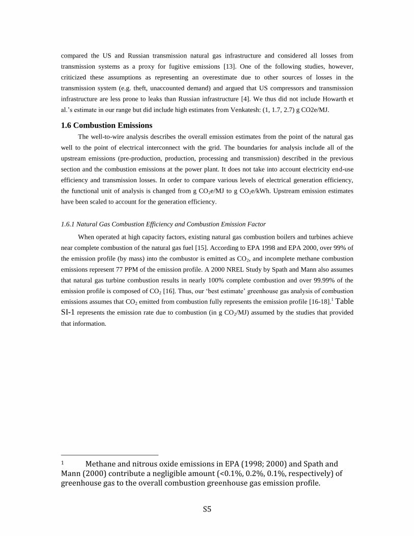
1.6.1 Natural Gas Combustion Efficiency and Combustion Emission Factor

When operated at high capacity factors, existing natural gas combustion boilers and turbines achieve

near complete combustion of the natural gas fuel [15]. According to EPA 1998 and EPA 2000, over 99% of

the emission profile (by mass) into the combustor is emitted as CO2, and incomplete methane combustion

emissions represent 77 PPM of the emission profile. A 2000 NREL Study by Spath and Mann also assumes

that natural gas turbine combustion results in nearly 100% complete combustion and over 99.99% of the

emission profile is composed of CO2 [16]. Thus, our ‘best estimate’ greenhouse gas analysis of combustion

emissions assumes that CO2 emitted from combustion fully represents the emission profile [16-18].1 Table

SI-1 represents the emission rate due to combustion (in g CO2/MJ) assumed by the studies that provided

that information.

1 Methane and nitrous oxide emissions in EPA (1998; 2000) and Spath and Mann (2000) contribute a negligible amount (<0.1%, 0.2%, 0.1%, respectively) of greenhouse gas to the overall combustion greenhouse gas emission profile.

S6

Table SI-1. Cited emissions factors for combusting

natural gas across the studies (LHV)

Emission Rate

(g CO2/MJ)

Hultman 57.1

Jiang 55.0

Stephenson 58.1

Burnham 56.6

Howarth 55.0

Average 56.3

1.6.2 Generation Efficiency Assumptions

Each study provided estimates of natural gas fired electricity generation efficiency values. For the

purposes of demonstrating the relative impact of increasing levels of generation efficiency on life cycle

emissions, we have grouped the efficiency factors into 4 categories that consider the overall performance of

the US natural gas fired generation fleet and marginal improvements in generation efficiency. All factors

have been converted (if necessary) to LHV basis.

Table SI-2. Power plant efficiencies cited in the studies for

current and future gas turbine technology, converted to LHV

Generation

Category Citation Generation Efficiency (%)

Current US

Average

Fleet

Jiang (Average Existing US Fleet) 47.3

NETL Current Gas Baseload 48.4

Stephenson (2009 EIA US Average Natural Gas) 47.6

Low

Efficiency

(Steam

Turbine or

Boiler)

Hultman (Average Current Conventional Gas

Turbine)

37.1

NETL Single Cycle Gas Turbine 30.1

Stephenson (2003 EIA Absolute Low

Efficiency)

31.0

Current US

Marginal

NGCC

Hultman (Average Conventional NGCC) 50.5

NETL Natural Gas Combined Cycle 50.2

Future

NGCC

Technology

Hultman Future High Efficiency 55.6

S7

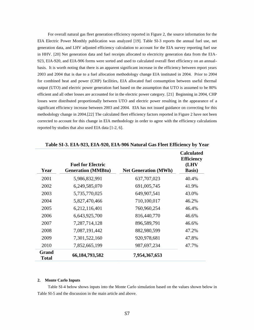
For overall natural gas fleet generation efficiency reported in Figure 2, the source information for the

EIA Electric Power Monthly publication was analyzed [19]. Table SI-3 reports the annual fuel use, net

generation data, and LHV adjusted efficiency calculation to account for the EIA survey reporting fuel use

in HHV. [20] Net generation data and fuel receipts allocated to electricity generation data from the EIA-

923, EIA-920, and EIA-906 forms were sorted and used to calculated overall fleet efficiency on an annual-

basis. It is worth noting that there is an apparent significant increase in the efficiency between report years

2003 and 2004 that is due to a fuel allocation methodology change EIA instituted in 2004. Prior to 2004

for combined heat and power (CHP) facilities, EIA allocated fuel consumption between useful thermal

output (UTO) and electric power generation fuel based on the assumption that UTO is assumed to be 80%

efficient and all other losses are accounted for in the electric power category. [21] Beginning in 2004, CHP

losses were distributed proportionally between UTO and electric power resulting in the appearance of a

significant efficiency increase between 2003 and 2004. EIA has not issued guidance on correcting for this

methodology change in 2004.[22] The calculated fleet efficiency factors reported in Figure 2 have not been

corrected to account for this change in EIA methodology in order to agree with the efficiency calculations

reported by studies that also used EIA data [1-2, 6].

Table SI-3. EIA-923, EIA-920, EIA-906 Natural Gas Fleet Efficiency by Year

Year

Fuel for Electric

Generation (MMBtu) Net Generation (MWh)

Calculated

Efficiency

(LHV

Basis)

2001 5,986,832,991 637,707,023 40.4%

2002 6,249,585,070 691,005,745 41.9%

2003 5,735,770,025 649,907,541 43.0%

2004 5,827,470,466 710,100,017 46.2%

2005 6,212,116,401 760,960,254 46.4%

2006 6,643,925,700 816,440,770 46.6%

2007 7,287,714,128 896,589,791 46.6%

2008 7,087,191,442 882,980,599 47.2%

2009 7,301,522,160 920,978,681 47.8%

2010 7,852,665,199 987,697,234 47.7%

Grand

Total 66,184,793,582 7,954,367,653

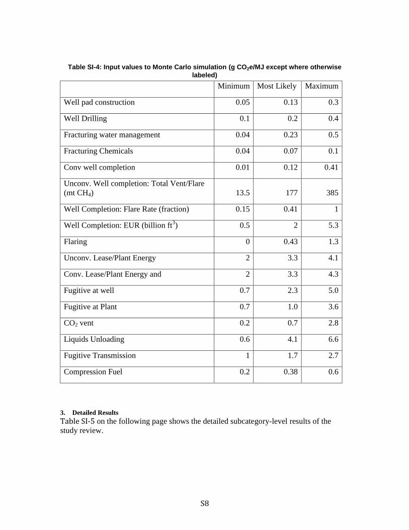
2. Monte Carlo Inputs

Table SI-4 below shows inputs into the Monte Carlo simulation based on the values shown below in

Table SI-5 and the discussion in the main article and above.

S8

Table SI-4: Input values to Monte Carlo simulation (g CO2e/MJ except where otherwise

labeled)

Minimum Most Likely Maximum

Well pad construction 0.05 0.13 0.3

Well Drilling 0.1 0.2 0.4

Fracturing water management 0.04 0.23 0.5

Fracturing Chemicals 0.04 0.07 0.1

Conv well completion 0.01 0.12 0.41

Unconv. Well completion: Total Vent/Flare

(mt CH4) 13.5 177 385

Well Completion: Flare Rate (fraction) 0.15 0.41 1

Well Completion: EUR (billion ft3) 0.5 2 5.3

Flaring 0 0.43 1.3

Unconv. Lease/Plant Energy 2 3.3 4.1

Conv. Lease/Plant Energy and 2 3.3 4.3

Fugitive at well 0.7 2.3 5.0

Fugitive at Plant 0.7 1.0 3.6

CO2 vent 0.2 0.7 2.8

Liquids Unloading 0.6 4.1 6.6

Fugitive Transmission 1 1.7 2.7

Compression Fuel 0.2 0.38 0.6

3. Detailed Results

Table SI-5 on the following page shows the detailed subcategory-level results of the

study review.

S9

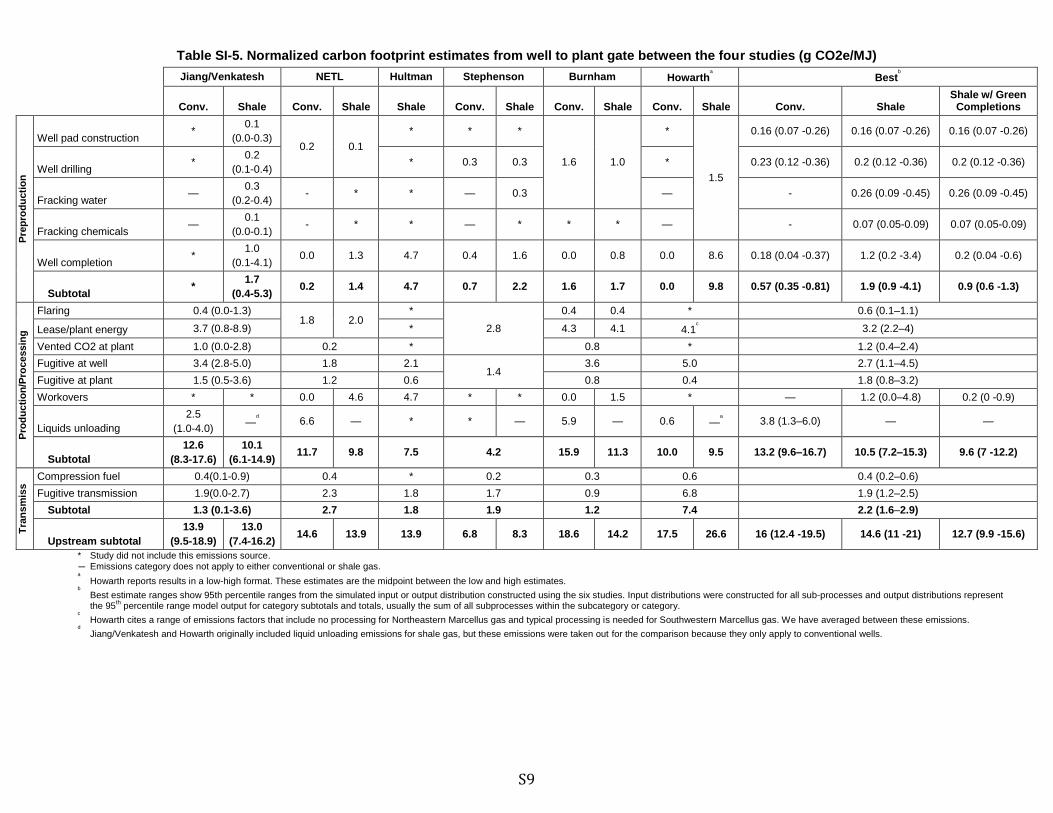
Table SI-5. Normalized carbon footprint estimates from well to plant gate between the four studies (g CO2e/MJ)

Jiang/Venkatesh NETL Hultman Stephenson Burnham Howartha

Bestb

Conv. Shale Conv. Shale Shale Conv. Shale Conv. Shale Conv. Shale Conv. Shale Shale w/ Green

Completions

Pre

pro

du

cti

on

Well pad construction *

0.1

(0.0-0.3) 0.2 0.1

* * *

1.6 1.0

*

1.5

0.16 (0.07 -0.26) 0.16 (0.07 -0.26) 0.16 (0.07 -0.26)

Well drilling *

0.2

(0.1-0.4) * 0.3 0.3 * 0.23 (0.12 -0.36) 0.2 (0.12 -0.36) 0.2 (0.12 -0.36)

Fracking water —

0.3

(0.2-0.4) - * * — 0.3 — - 0.26 (0.09 -0.45) 0.26 (0.09 -0.45)

Fracking chemicals —

0.1

(0.0-0.1) - * * — * * * — - 0.07 (0.05-0.09) 0.07 (0.05-0.09)

Well completion *

1.0

(0.1-4.1) 0.0 1.3 4.7 0.4 1.6 0.0 0.8 0.0 8.6 0.18 (0.04 -0.37) 1.2 (0.2 -3.4) 0.2 (0.04 -0.6)

Subtotal *

1.7

(0.4-5.3) 0.2 1.4 4.7 0.7 2.2 1.6 1.7 0.0 9.8 0.57 (0.35 -0.81) 1.9 (0.9 -4.1) 0.9 (0.6 -1.3)

Pro

du

cti

on

/Pro

ce

ss

ing

Flaring 0.4 (0.0-1.3) 1.8 2.0

*

2.8

0.4 0.4 * 0.6 (0.1–1.1)

Lease/plant energy 3.7 (0.8-8.9) * 4.3 4.1 4.1c

3.2 (2.2–4)

Vented CO2 at plant 1.0 (0.0-2.8) 0.2 * 0.8 * 1.2 (0.4–2.4)

Fugitive at well 3.4 (2.8-5.0) 1.8 2.1 1.4

3.6 5.0 2.7 (1.1–4.5)

Fugitive at plant 1.5 (0.5-3.6) 1.2 0.6 0.8 0.4 1.8 (0.8–3.2)

Workovers * * 0.0 4.6 4.7 * * 0.0 1.5 * — 1.2 (0.0–4.8) 0.2 (0 -0.9)

Liquids unloading

2.5

(1.0-4.0) —

d

6.6 — * * — 5.9 — 0.6 —a

3.8 (1.3–6.0) — —

Subtotal

12.6

(8.3-17.6)

10.1

(6.1-14.9) 11.7 9.8 7.5 4.2 15.9 11.3 10.0 9.5 13.2 (9.6–16.7) 10.5 (7.2–15.3) 9.6 (7 -12.2)

Tra

ns

mis

s Compression fuel 0.4(0.1-0.9) 0.4 * 0.2 0.3 0.6 0.4 (0.2–0.6)

Fugitive transmission 1.9(0.0-2.7) 2.3 1.8 1.7 0.9 6.8 1.9 (1.2–2.5)

Subtotal 1.3 (0.1-3.6) 2.7 1.8 1.9 1.2 7.4 2.2 (1.6–2.9)

Upstream subtotal

13.9

(9.5-18.9)

13.0

(7.4-16.2) 14.6 13.9 13.9 6.8 8.3 18.6 14.2 17.5 26.6 16 (12.4 -19.5) 14.6 (11 -21) 12.7 (9.9 -15.6)

* Study did not include this emissions source. — Emissions category does not apply to either conventional or shale gas. a

Howarth reports results in a low-high format. These estimates are the midpoint between the low and high estimates. b

Best estimate ranges show 95th percentile ranges from the simulated input or output distribution constructed using the six studies. Input distributions were constructed for all sub-processes and output distributions represent the 95

th percentile range model output for category subtotals and totals, usually the sum of all subprocesses within the subcategory or category.

c

Howarth cites a range of emissions factors that include no processing for Northeastern Marcellus gas and typical processing is needed for Southwestern Marcellus gas. We have averaged between these emissions. d

Jiang/Venkatesh and Howarth originally included liquid unloading emissions for shale gas, but these emissions were taken out for the comparison because they only apply to conventional wells.

S10

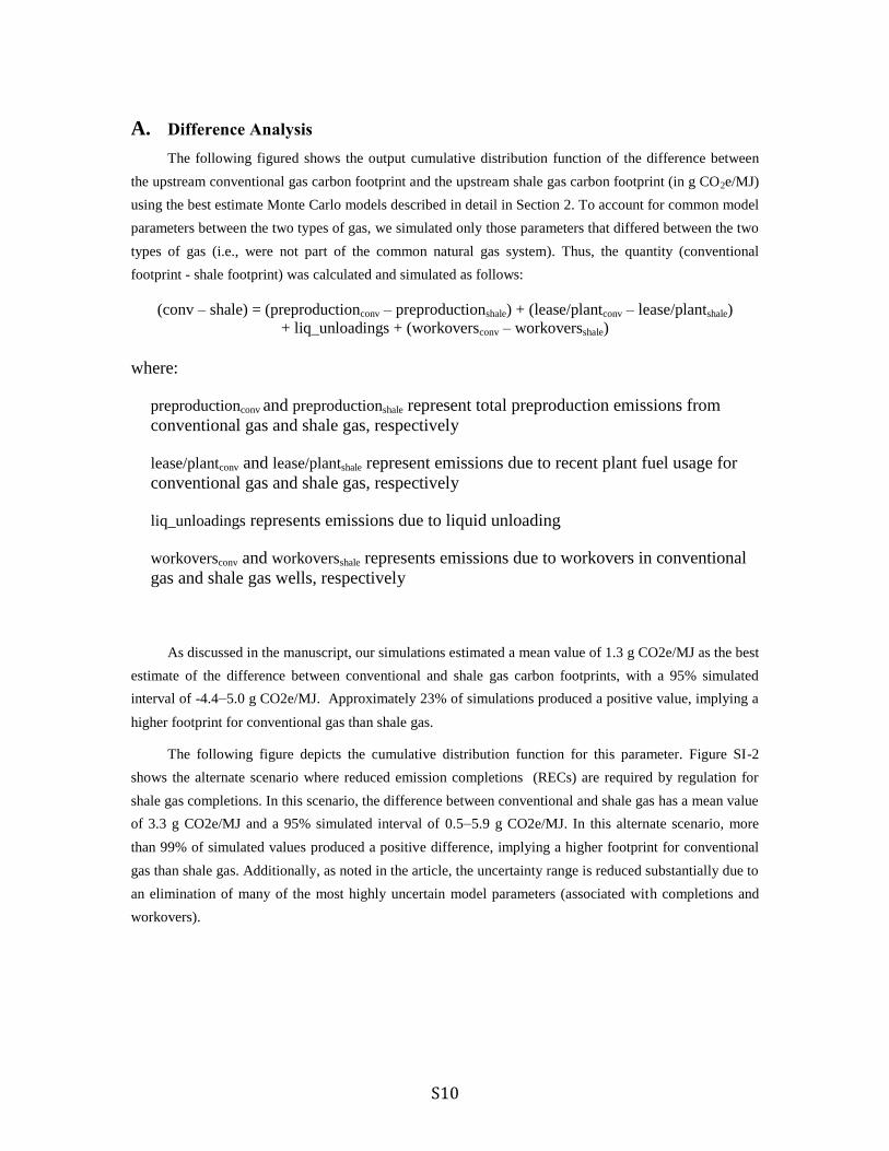
A. Difference Analysis

The following figured shows the output cumulative distribution function of the difference between

the upstream conventional gas carbon footprint and the upstream shale gas carbon footprint (in g CO2e/MJ)

using the best estimate Monte Carlo models described in detail in Section 2. To account for common model

parameters between the two types of gas, we simulated only those parameters that differed between the two

types of gas (i.e., were not part of the common natural gas system). Thus, the quantity (conventional

footprint - shale footprint) was calculated and simulated as follows:

(conv – shale) = (preproductionconv – preproductionshale) + (lease/plantconv – lease/plantshale)

+ liq_unloadings + (workoversconv – workoversshale)

where:

preproductionconv and preproductionshale represent total preproduction emissions from

conventional gas and shale gas, respectively

lease/plantconv and lease/plantshale represent emissions due to recent plant fuel usage for

conventional gas and shale gas, respectively

liq_unloadings represents emissions due to liquid unloading

workoversconv and workoversshale represents emissions due to workovers in conventional

gas and shale gas wells, respectively

As discussed in the manuscript, our simulations estimated a mean value of 1.3 g CO2e/MJ as the best

estimate of the difference between conventional and shale gas carbon footprints, with a 95% simulated

interval of -4.4–5.0 g CO2e/MJ. Approximately 23% of simulations produced a positive value, implying a

higher footprint for conventional gas than shale gas.

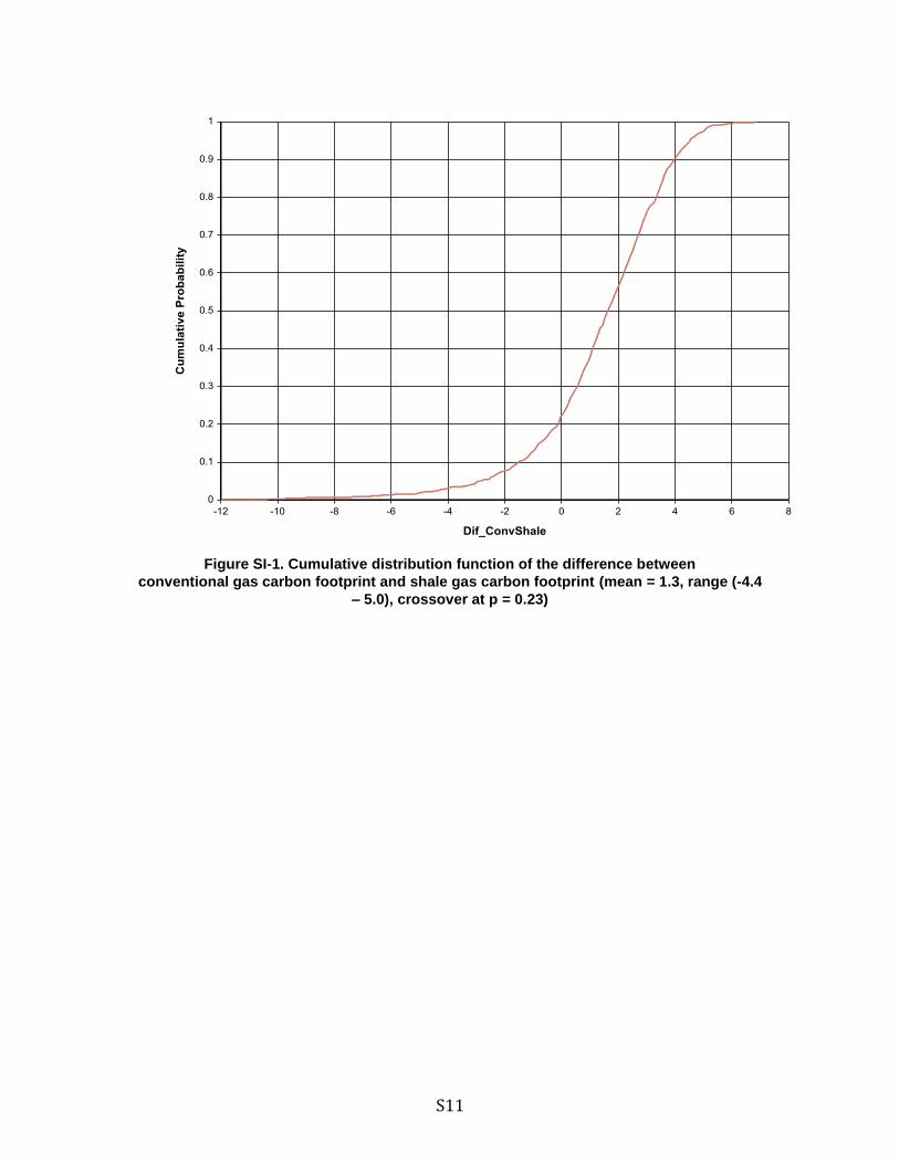
The following figure depicts the cumulative distribution function for this parameter. Figure SI-2

shows the alternate scenario where reduced emission completions (RECs) are required by regulation for

shale gas completions. In this scenario, the difference between conventional and shale gas has a mean value

of 3.3 g CO2e/MJ and a 95% simulated interval of 0.5–5.9 g CO2e/MJ. In this alternate scenario, more

than 99% of simulated values produced a positive difference, implying a higher footprint for conventional

gas than shale gas. Additionally, as noted in the article, the uncertainty range is reduced substantially due to

an elimination of many of the most highly uncertain model parameters (associated with completions and

workovers).

S11

Figure SI-1. Cumulative distribution function of the difference between

conventional gas carbon footprint and shale gas carbon footprint (mean = 1.3, range (-4.4

– 5.0), crossover at p = 0.23)

S12

Figure SI-2. Cumulative distribution function of the difference between

conventional gas carbon footprint and shale gas carbon footprint for

scenario where green completions are required (mean = 3.3, range (0.5 – 5.9), crossover at

p < 0.01)

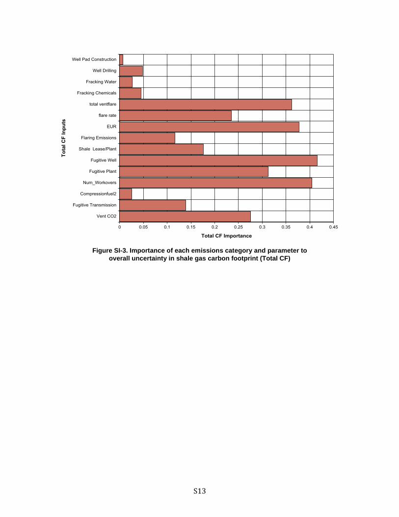
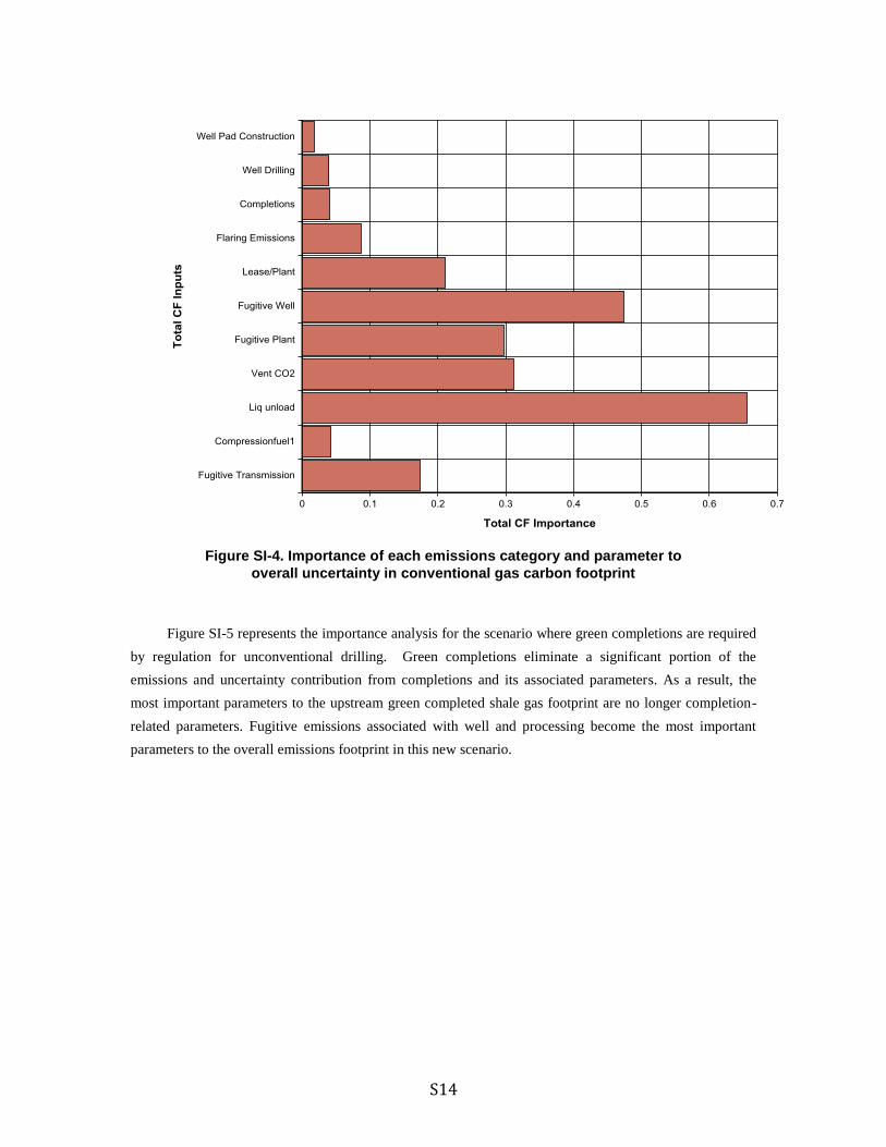
B. Importance Analysis

The following two figures show the importance of individual model parameters to overall upstream

carbon footprint uncertainty for shale gas (Figure SI-3) and conventional gas (Figure SI-4). Importance is

calculated as the rank order correlation coefficient between the samples of an input distribution and the

output distribution for total carbon footprint for either shale or conventional gas. A higher value of this

parameter means that the input parameter contributes more to the overall carbon footprint uncertainty. As

Figure SI-3 shows, the parameters that are the most important to upstream shale gas carbon footprint

uncertainty are the number of workovers per well lifetime (workovers), the fugitive emissions at the well

(fugitive well), the estimated ultimate recovery per well (EUR), and the total gas released during well

completion and workovers (total ventflare). The parameters most important to upstream conventional gas

footprint uncertainty are emissions related to liquid unloading (liq unload), fugitive emissions at the well

(fugitive well), and the fugitive emissions at the processing plant (fugitive plant).

S13

Figure SI-3. Importance of each emissions category and parameter to

overall uncertainty in shale gas carbon footprint (Total CF)

S14

Figure SI-4. Importance of each emissions category and parameter to

overall uncertainty in conventional gas carbon footprint

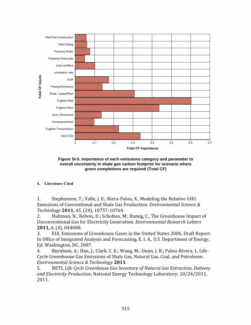
Figure SI-5 represents the importance analysis for the scenario where green completions are required

by regulation for unconventional drilling. Green completions eliminate a significant portion of the

emissions and uncertainty contribution from completions and its associated parameters. As a result, the

most important parameters to the upstream green completed shale gas footprint are no longer completion-

related parameters. Fugitive emissions associated with well and processing become the most important

parameters to the overall emissions footprint in this new scenario.

S15

Figure SI-5. Importance of each emissions category and parameter to

overall uncertainty in shale gas carbon footprint for scenario where

green completions are required (Total CF)

4. Literature Cited

1. Stephenson, T.; Valle, J. E.; Riera-Palou, X., Modeling the Relative GHG Emissions of Conventional and Shale Gas Production. Environmental Science & Technology 2011, 45, (24), 10757-10764. 2. Hultman, N.; Rebois, D.; Scholten, M.; Ramig, C., The Greenhouse Impact of Unconventional Gas for Electricity Generation. Environmental Research Letters 2011, 6, (4), 044008. 3. EIA, Emissions of Greenhouse Gases in the United States 2006, Draft Report. In Office of Integrated Analysis and Forecasting, E. I. A., U.S. Department of Energy, Ed. Washington, DC, 2007. 4. Burnham, A.; Han, J.; Clark, C. E.; Wang, M.; Dunn, J. B.; Palou-Rivera, I., Life-Cycle Greenhouse Gas Emissions of Shale Gas, Natural Gas, Coal, and Petroleum. Environmental Science & Technology 2011. 5. NETL Life Cycle Greenhouse Gas Inventory of Natural Gas Extraction, Delivery and Electricity Production; National Energy Technology Laboratory: 10/24/2011, 2011.

S16

6. Venkatesh, A.; Jaramillo, P.; Griffin, W. M.; Matthews, H. S., Uncertainty in Life Cycle Greenhouse Gas Emissions from United States Natural Gas End-Uses and its Effects on Policy. Environmental Science & Technology 2011, 45, (19), 8182-8189. 7. EPA Greenhouse Gas Emissions Reporting from the Petroleum and Natural Gas Industry: Background Technical Support Document; US Environmental Protection Agency: Washington, DC, 2011; pp 1-144. 8. GAO Federal Oil and Gas Leases: Opportunities Exist to Capture Vented and Flared Natural Gas, Which Would Increase Royalty Payments and Reduce Greenhouse Gases; Government Accountability Office: Washington, DC, 2010. 9. EPA, Oil and Natural Gas Sector: New Source Performance Standards and National Emission Standards for Hazardous Air Pollutants Reviews. In EPA, Ed. FR: Washington, 2011; Vol. 76, pp 52738-52843. 10. Santoro, R. L.; Howarth, R. H.; Ingraffea, A. R. Indirect Emissions of Carbon Dioxide from Marcellus Shale Gas Development; Agriculture, Energy, and Environment Program at Cornell University: Washington, DC, 2011; pp 1-28. 11. Wang, M. GREET 1.5 - Transportation Fuel-Cycle Model, Volume 1: Methodology, Development, Use, and Results; Argonne National Laboratory, Center for Transportation Research, Energy Systems Division: Argonne National Laboratory, 1999. 12. API Compendium of Greenhouse Gas Emissions Methodologies for the Oil and Natural Gas Industry; American Petroleum Institute: Washington, 8/2009, 2009. 13. Howarth, R.; Santoro, R.; Ingraffea, A., Methane and the greenhouse-gas footprint of natural gas from shale formations. Climatic Change 2011, 106, (4), 679-690. 14. Harrison, M. R.; Shires, T. M.; Wessels, J. K.; Cowgill, R. M. Methane Emissions from the Natural Gas Industry; National Risk Management Research Laboratory: 1996. 15. EPA AP 42 Compilation of Air Pollutant Emission Factors; US Environmental Protection Agency: Washington, DC, 2009. 16. Spath, P. L.; Mann, M. K. Life Cycle Assessment of a Natural Gas Combined-Cycle Power Generation System; National Renewable Energy Laboratory: Golden, CO, 2000; pp 1-56. 17. EPA AP 42 Compilation of Air Pollutant Emission Factors, Chapter 1.4: Natural Gas Combustion; US Environmental Protection Agency: Washington, DC, 1998. 18. EPA AP 42 Compilation of Air Pollutant Emission Factors, Chapter 3.1: Stationary Gas Turbines; US Environmental Protection Agency: Washington, DC, 2000. 19. EIA Form EIA-906, EIA-920, and EIA-923 Data. http://www.eia.gov/cneaf/electricity/page/eia906_920.html (January 9), 20. EIA, Form EIA-923 Power Plant Operations Report Instrucitons. In EIA, Ed. Washington, 2011; p 10. 21. EIA, Electric Power Monthly January 2012: Appendix C Technical Notes. In EIA: Washington, 2012; p 165. 22. Wirman, C., Personal Communication. In Clavin, C., Ed. Washington, 2011.