Life Cycle Cost Manual for the Federal Energy Management

NIST Handbook 135 2020 Edition

LIFE CYCLE COSTING MANUAL for the Federal Energy Management

Program

Joshua Kneifel David Webb

This publication is available free of charge from: https://doi.org/10.6028/NIST.HB.135-2020

NIST Handbook 135 2020 Edition

LIFE CYCLE COSTING MANUAL for the Federal Energy Management

Program

Joshua Kneifel David Webb

Applied Economics Office Engineering Laboratory

This publication is available free of charge from: https://doi.org/10.6028/NIST.HB.135-2020

September 2020 Supersedes NIST Handbook 135 (1995 Revision)

Prepared for: U.S. Department of Energy

Federal Energy Management Program Washington, DC 20585

U.S. Department of Commerce Wilbur L. Ross, Jr., Secretary

National Institute of Standards and Technology Walter Copan, NIST Director and Undersecretary of Commerce for Standards and Technology

Certain commercial entities, equipment, or materials may be identified in this document to describe an experimental procedure or concept adequately.

Such identification is not intended to imply recommendation or endorsement by the National Institute of Standards and Technology, nor is it intended to imply that the entities, materials, or equipment are necessarily the best available for the purpose.

National Institute of Standards and Technology Handbook 135 (2020 Edition) Natl. Inst. Stand. Technol. Handbook 135-2020, 295 pages (September 2020)

This publication is available free of charge from:https://doi.org/10.6028/NIST.HB.135-2020

iii

This p

ublica

tion is ava

ilab

le free

of ch

arge

from: h

ttps://doi.o

rg/1

0.6

028

/NIS

T.H

B.13

5-202

0

Abstract

Handbook 135 is a guide to understanding the life cycle cost (LCC) methodology and criteria established by the Federal Energy Management Program (FEMP) for the economic evaluation of high-performance facility projects, including energy efficiency, water conservation, and renewable energy projects in all federal facilities. It expands on the life cycle cost methods and criteria contained in the FEMP rules published in 10 CFR 436, Subpart A, which applies to all federal agencies. The purpose of this handbook is to facilitate the implementation of the FEMP rules by explaining the LCC method, defining the measures of economic performance used, describing the assumptions and procedures to follow in performing evaluations, giving examples, and noting NIST computer software available for computation and reporting purposes. An annual supplement to Handbook 135, Energy Price Indices and Discount Factors for LCC Analysis, NISTIR 85-3273, is also published by NIST to provide the current discount rate, discount factors, and energy escalation factors used for conducting an LCC analysis in accordance with the FEMP rules. This annual supplement is required when using Handbook 135 and is used in updating NIST LCC-related software.

This new edition of Handbook 135 replaces the 1995 version. The new edition is extensively revised and organized around the key steps in an LCC analysis. Although the underlying LCC methodology has not changed, the content of the handbook has been updated to include the most relevant information. Given the technological developments since its 1995 release, the manual worksheets previously provided for completing LCC analysis have been removed. The examples have been updated and expanded to provide explicit use cases for projects with a broader scope than energy efficiency and water conservation to include all considerations of high-performance facilities, including sustainability and resilience. Additionally, the handbook provides additional information resources (e.g., data sources, requirements, codes and standards, and guidance by project goal). The handbook will be updated on an ad hoc basis dependent on future changes in federal statutes and regulations, agency goals and guidance, LCCA support resource development, and available funding.

Keywords

benefit-cost analysis; building economics; building technology; capital investment; cost-effectiveness; economic analysis; energy conservation; energy economics; life cycle cost analysis; public buildings; renewable energy; water conservation; sustainability; resilience

iv

This p

ublica

tion is ava

ilab

le free

of ch

arge

from: h

ttps://doi.o

rg/1

0.6

028

/NIS

T.H

B.13

5-202

0

v

This p

ublica

tion is ava

ilab

le free

of ch

arge

from: h

ttps://doi.o

rg/1

0.6

028

/NIS

T.H

B.13

5-202

0

Preface Why a New Edition of Handbook 135?

This manuscript was developed by the Applied Economics Office (AEO) in the Engineering Laboratory (EL) at the National Institute of Standards and Technology (NIST) for the U.S. Department of Energy (DOE) Federal Energy Management Program (FEMP). Handbook 135 was developed for use in performing life-cycle cost analysis (LCCA) of investments in energy and water conservation projects and renewable energy resource projects for federal buildings and facilities. DOE FEMP has codified the rules for performing LCCA of such investments in the Code of Federal Regulations (CFR), 10 CFR 436, Subpart A, Methodology and Procedures for Life Cycle Cost Analysis (CFR, 2018). These rules apply to both new and existing facilities owned or leased by the federal government. These economic evaluations are required by the Federal Energy Management Improvement Act of 1988 (S.1382, 1988) and the National Energy Conservation Policy Act (NECPA) of 1978 (H.R.5037, 1978). NECPA allows projects to use publicly appropriated funds, private financing such as energy savings performance contracts (ESPCs) or utility energy service contracts (UESC), or some combination of the two. NECPA was amended by the Energy Policy Act (EPACT) of 1992 (H.R.776, 1992), which included the addition of water and renewable energy to the federal energy management section.

Since the last edition of Handbook 135 was published in 1995, multiple legislative initiatives have been enacted and executive actions have been implemented (and superseded). These have expanded the focus beyond energy efficiency and water conservation projects.

Executive Order (EO) 13123 (E.O.13123, 1999), "Greening the Government through Efficient Energy Management," introduced a focus on more sustainable government operations through life-cycle cost-effective projects. Goals include reducing water consumption, greenhouse gas emissions, reducing energy (specifically petroleum) consumption, and increasing renewable energy production at federal facilities. FEMP, with NIST’s assistance, provided guidance to “clarify how agencies determine the life-cycle cost for investments required by the Order" (Sec 502) – “Guidance on Life-Cycle Cost Analysis Required by Executive Order 13123” (FEMP, 2005).

EPACT of 2005 (H.R.6, 2005) amended NECPA to set new baselines and energy consumption reduction and energy-efficient product requirements, expanded the maximum period over which to complete an LCCA to 40 years, and provided the ability to “bundle individual measures of varying paybacks.”

EO 13423 (E.O.13423, 2007), “Strengthening Federal Environmental, Energy, and Transportation Management,” replaced EO 13123 and instructed federal agencies to “conduct their environmental, transportation, and energy-related activities under the law in support of their respective missions in an environmentally, economically and fiscally sound, integrated, continuously improving, efficient, and sustainable manner.” Specific

vi

This p

ublica

tion is ava

ilab

le free

of ch

arge

from: h

ttps://doi.o

rg/1

0.6

028

/NIS

T.H

B.13

5-202

0

goals expanded to include energy efficiency, acquisitions, renewable energy, sustainable buildings, water conservation, fleets (i.e., vehicles), recycling, toxic chemical reduction, and electronics stewardship.

EO 13693 (E.O.13693, 2015), "Planning for Federal Sustainability in the Next Decade," replaced EO 13423 and stated “Federal agencies shall promote life-cycle cost-effective building energy efficiency, water conservation, renewable energy, and fleet efficiency.”

EO 13834 (E.O.13834, 2018) – “Efficient Federal Operations” – has replaced EO 13693 and continues similar underlying goals. Section 1 states that “agencies shall meet such statutory requirements in a manner that increases efficiency, optimizes performance, eliminates unnecessary use of resources, and protects the environment…each agency shall prioritize actions that reduce waste, cut costs, enhance the resilience of Federal infrastructure and operations, and enable more effective accomplishment of its mission.” Section 2 lists the goals for agencies:

Achieve and maintain annual reductions in building energy use and implement energy efficiency measures that reduce costs

Meet statutory requirements relating to the consumption of renewable energy and electricity

Reduce potable and non-potable water consumption, and comply with storm water management requirements

Utilize performance contracting to achieve energy, water, building modernization, and infrastructure goals

Ensure that new construction and major renovations conform to applicable building energy efficiency requirements and sustainable design principles consider building efficiency when renewing or entering leases; implement space utilization and optimization practices; and annually assess and report on building conformance to sustainability metrics

Implement waste prevention and recycling measures and comply with all Federal requirements regarding solid, hazardous, and toxic waste management and disposal

Acquire, use, and dispose of products and services, including electronics, in accordance with statutory mandates for purchasing preference, Federal Acquisition Regulation requirements, and other applicable Federal procurement policies

Track and, as required by section 7(b) of this order, report on energy management activities, performance improvements, cost reductions, greenhouse gas emissions, energy and water savings, and other appropriate performance measures.

A request from the Office of Management and Budget (OMB) has been made for FEMP to update the EO 13834 guidance for consistency with EO 13123, including referencing the new EO and incorporating “OMB/CEQ direction per EO 13834 Implementation Instructions.”

vii

This p

ublica

tion is ava

ilab

le free

of ch

arge

from: h

ttps://doi.o

rg/1

0.6

028

/NIS

T.H

B.13

5-202

0

Implementing instructions from the Council on Environmental Quality (CEQ) for EO 13834 were published in April 2019 (CEQ, 2019b). All three implementation actions listed in the instructions are relevant and support the update of this handbook:

To facilitate efficient implementation, progress tracking, and performance measurement, CEQ and OMB will coordinate with FEMP and GSA on an ongoing basis to identify opportunities to 1) further streamline data collection, 2) improve reporting and data analysis, 3) use data to inform cost-effective implementation, and 4) quantify cost savings.

FEMP, in coordination with other agencies, as appropriate, should identify or develop tools and methodologies to assist agencies in developing progress milestones and projections for facility energy, water, performance contracting, and sustainable building goals.

Agencies that provide government-wide technical support and information for federal energy and environmental performance, including FEMP, GSA, EPA, and USDA, should ensure that relevant materials, trainings, and web resources are reviewed and regularly updated, as appropriate, to provide current information with regard to federal policies, priorities, guidance, and best management practices.

CEQ (2019b) defines current sustainability goals organized into three categories: building efficiency and management, fleet management, and cross-cutting goals. Building efficiency and management includes seven subcategories: (1) energy reduction, (2) renewable energy, (3) water management, (4) performance contracting, (5) sustainable buildings, (6) waste management, and (7) building evaluations, benchmarking, and energy management. Cross-cutting goals include acquisition, electronics stewardship, data center management, and greenhouse gas management and reporting.

This handbook will touch on many of these topics, including how to apply life-cycle cost analysis when choosing the most cost-effective measures to meet each goal below specified in CEQ (2019b):

Achieve 30 % reduction in energy use intensity (EUI) relative to FY2003, and annual progress each fiscal year

Consume at least 7.5 % electricity from renewable sources

Achieve 20 % reduction in potable and non-potable water relative to FY2007, and annual progress each fiscal year

Utilize performance contracting where life-cycle cost-effective to achieve energy, water, and building modernization, and infrastructure goals

Ensure that at least 15 % of buildings or gross area qualifies as sustainable, and annual progress is made each fiscal year.

viii

This p

ublica

tion is ava

ilab

le free

of ch

arge

from: h

ttps://doi.o

rg/1

0.6

028

/NIS

T.H

B.13

5-202

0

These goals will be discussed in more detail, including one or more examples in Chapter 11 through Chapter 15. Waste management, fleet management, acquisition, and electronics are excluded because they are outside the scope of this handbook.

The CEQ Resources and Guidance for Federal Agencies webpage (CEQ, 2019c) provides guidance documents to assist agencies in sustainability policy and program implementation for a range of topics, including sustainable federal buildings, renewable energy, water efficiency, sustainable locations, and greenhouse gas (GHG) accounting and reporting. According to CEQ (2019c), “Guidance documents issued under prior Executive Orders are under review and may be revised. Federal agencies may continue to refer to this guidance, unless revised or revoked, particularly regarding established procedures, reporting processes, definitions, and technical matters.” This document references the guidance documents available as of June 10, 2019.

The most recent EO (13834) has built on prior EOs to further expand the scope for which LCCA is to be applied by federal agencies since the last version of the handbook was published in 1995. It goes beyond energy efficiency and water conservation to include environmental impact reduction, sustainability, resilience, and space utilization of buildings and other infrastructure.

This 2020 edition of NIST Handbook 135, Life Cycle Costing Manual for the Federal Energy Management Program, represents a major revision of earlier versions. Handbook 135 was originally published in 1980 and last revised in 1995. The numerous legislative and executive actions since 1995 have impacted the appropriate guidance to be provided by FEMP. This new edition incorporates changes in the FEMP rules for performing life-cycle cost analysis of energy and water conservation projects in federal buildings/facilities and expands the scope of the discussion to include broader federal goals of high-performance buildings/facilities, incorporating renewable energy, environmental stewardship, sustainability, resilience, and space utilization optimization of buildings. The principal changes in the rules and scope since the last edition are:

The maximum study period has been extended from 25 years to 40 years.

Broadening of scope to include environmental, sustainability, resilience, and space utilization projects including those identified in EO 13834

More detailed consideration of funding options including energy savings performance contracts (ESPCs) and “bundling” of projects

Reconsideration of options available for estimating residual value

Greater discussion of difficult-to-value and/or non-monetary benefits and costs

Greater discussion of uncertainty

Greater focus on considerations for whole building evaluation

List of resources for additional details on specific topics

New examples explaining how to evaluate new project goals (e.g., resilience)

ix

This p

ublica

tion is ava

ilab

le free

of ch

arge

from: h

ttps://doi.o

rg/1

0.6

028

/NIS

T.H

B.13

5-202

0

The subject matter in this new edition maintains the same step-by-step procedures for performing an LCCA included in the previous version. Rather than emphasizing the theoretical underpinnings of benefit-cost analysis in general, we have tried to include and emphasize topics of practical value to analysts who are called upon to perform economic analysis of building performance improvement projects using the FEMP methodology. In this attempt, we have benefited greatly from the questions and comments received from participants in a FEMP-sponsored LCC workshop that we conducted in early 2018.

The treatment of LCCA in this handbook is directed towards engineers and architects, energy analysts and managers, and budget analysts and planners of federally owned facilities. The handbook is also intended for managers who need to interpret LCC studies performed by contractors or other analysts and make decisions based upon them. Even though the emphasis of the handbook is explaining and amplifying the FEMP LCC requirements for the economic evaluation of building performance improvement projects in federal buildings, the underlying methodology is based on general economic theory and is generic enough to be useful for LCC analyses in the private sector as well.

DOE has actively consulted with and received substantial assistance from the National Institute of Standards and Technology (NIST) in developing and amending the FEMP LCC rules. In addition, for over 30 years NIST has provided significant technical assistance to DOE in support of the FEMP LCC methodology, including the publication of this handbook and the “Annual Supplement to Handbook 135,” the development of supporting software, and teaching LCC workshops for federal energy managers and other interested participants at many locations throughout the United States.

FEMP life-cycle costing methods and procedures set forth in 10 CFR 436, Subpart A, are to be followed by all federal agencies, unless specifically exempted, in evaluating the cost-effectiveness of potential energy and water conservation projects and renewable energy projects in federally owned and leased buildings. To the extent possible, these projects should be evaluated separately from non-energy and non-water-related projects in federal buildings. The current FEMP discount rate for energy- and water-related projects is published in the “Annual Supplement to Handbook 135, Energy Price Indices and Discount Factors for Life- Cycle Cost Analysis,” which is updated annually at the beginning of the federal fiscal year.

While this handbook focuses on the requirements of the FEMP LCC rules as they apply to federal buildings and facilities, the LCC methodology presented is entirely consistent with ASTM International standards on building economics, including:

E917 Practice for Measuring Life-cycle Costs of Buildings and Building Systems (ASTM, 2017a)

E964 Practice for Measuring Benefit-to-Cost and Savings-to-Investment Ratios for Buildings and Building Systems (ASTM, 2017b)

E1057 Practice for Measuring Internal Rate and Adjusted Internal Rate of Return for Investments in Buildings and Building Systems (ASTM, 2017c)

x

This p

ublica

tion is ava

ilab

le free

of ch

arge

from: h

ttps://doi.o

rg/1

0.6

028

/NIS

T.H

B.13

5-202

0

E1074 Practice for Measuring Net Benefits for Investments in Buildings and Building Systems (ASTM, 2017d)

E1121 Practice for Measuring Payback for Investments in Buildings and Building Systems (ASTM, 2017e)

E1185 Standard Guide for Selecting Economic Methods for Evaluating Investments in Buildings and Building Systems (ASTM, 2017f)

E1369 Standard Guide for Selecting Techniques for Treating Uncertainty and Risk in the Economic Evaluation of Buildings and Building Systems (ASTM, 2015)

LCC-Supporting Publications and Training

As called for by NECPA, NIST has provided technical assistance to DOE FEMP in formulating LCC methods, handbooks, energy price and discount factors, and software for economic analysis of energy and water conservation and renewable energy projects in the federal government. Along with Handbook 135, NIST has developed other resources in support of FEMP:

(1) “Energy Price Indices and Discount Factors for Life- Cycle Cost Analysis - XXXX, National Institute of Standards and Technology, NISTIR 85-3273-X.” This report, updated annually, provides energy price indices and discount factor multipliers needed to estimate the present value of energy and other future costs. The data are based on energy price projections developed by the Energy Information Administration (EIA) of the DOE. Users of Handbook 135 will need the most recent version of this report to perform LCC analyses for federal projects. This report is referenced throughout this manual as the “Annual Supplement to Handbook 135.”

(2) The NIST "Building Life Cycle Cost" (BLCC) Software (NIST, 2006a). The BLCC software serves as the primary support software for Handbook 135. This software is updated annually to incorporate the most recent changes in discount rates and EIA energy price escalation rates. For more information on this software, see Chapter 16.

(3) Energy Escalation Rate Calculator (EERC) (NIST, 2006b). EERC is a software for calculating average escalation rates for different fuel types based on a location, industry, study period, and inflation rate. For more information on this software, see Chapter 16.

These software and related documents are available, free of charge, on FEMP’s BLCC webpage: http://energy.gov/eere/femp/building-life cycle-cost-programs

FEMP and NIST agreed to stop conducting LCCA workshops after 2008, and instead provide a list of FEMP-certified LCC trainers, which is available upon request to FEMP. Prior training included in the workshops introduced the LCC method and LCC software. An introduction to the FEMP LCC methods is available at the Whole Building Design Guide webpage: https://www.wbdg.org/resources/life cycle-cost-analysis-lcca.

xi

This p

ublica

tion is ava

ilab

le free

of ch

arge

from: h

ttps://doi.o

rg/1

0.6

028

/NIS

T.H

B.13

5-202

0

Further Information

Further information on the FEMP can be obtained from the FEMP staff, Office of the Assistant Secretary for Energy Efficiency and Renewable Energy, U.S. Department of Energy. Though aimed primarily at supporting FEMP, LCC methods and criteria, these resources can also be used by state and local governments and the private sector for conducting LCC analysis of buildings and building systems. The NIST LCC software is adaptable to FEMP LCC criteria, OMB Circular A-94 criteria, military construction (MILCON), and general LCC analysis.

xii

This p

ublica

tion is ava

ilab

le free

of ch

arge

from: h

ttps://doi.o

rg/1

0.6

028

/NIS

T.H

B.13

5-202

0

xiii

This p

ublica

tion is ava

ilab

le free

of ch

arge

from: h

ttps://doi.o

rg/1

0.6

028

/NIS

T.H

B.13

5-202

0

Disclaimers

The policy of the National Institute of Standards and Technology is to use metric units in all its published materials. Because this report is intended for the U.S. construction industry, which uses U.S. customary units, it is more practical and less confusing to include U.S. customary units as well as metric units. Measurement values in this report are therefore stated in metric units first, followed by the corresponding values in U.S. customary units within parentheses.

Certain commercial entities, equipment, or materials may be identified in this document to describe an experimental procedure or concept adequately. Such identification is not intended to imply recommendation or endorsement by the National Institute of Standards and Technology, nor is it intended to imply that the entities, materials, or equipment are necessarily the best available for the purpose.

xiv

This p

ublica

tion is ava

ilab

le free

of ch

arge

from: h

ttps://doi.o

rg/1

0.6

028

/NIS

T.H

B.13

5-202

0

xv

This p

ublica

tion is ava

ilab

le free

of ch

arge

from: h

ttps://doi.o

rg/1

0.6

028

/NIS

T.H

B.13

5-202

0

Acknowledgements

The authors wish to thank all those who contributed ideas and suggestions for this handbook. Dr. David Butry, Chief, Applied Economics Office (AEO), Engineering Laboratory (EL), NIST, who reviewed the final manuscript, for his helpful comments and suggestions. Dr. Cheyney O’Fallon (AEO), EL, NIST, who reviewed the draft and suggested improvements. Phil Coleman at DOE, for his detailed comments and suggestions. Other federal agency reviewers, including Kurmit Rockwell, Thomas Hattery, Christine Walker, and Robert Slattery at DOE, Kinga Porst-Hydras at GSA, and Alexander Zhivov at USACE, for their comments and suggestions. Sieglinde K. Fuller and Stephen R. Petersen, who wrote the 1995 edition of this handbook. The U.S. Department of Energy, Federal Energy Management Program, for its support and direction of this work.

Author Information

Joshua Kneifel Economist National Institute of Standards and Technology Engineering Laboratory 100 Bureau Drive, Mailstop 8603 Gaithersburg, MD 20899 8603 Tel.: 301-975-6857 Email: [email protected] David Webb Economist National Institute of Standards and Technology Engineering Laboratory 100 Bureau Drive, Mailstop 8603 Gaithersburg, MD 20899 8603 Tel.: 301-975-2644 Email: [email protected]

xvi

This p

ublica

tion is ava

ilab

le free

of ch

arge

from: h

ttps://doi.o

rg/1

0.6

028

/NIS

T.H

B.13

5-202

0

xvii

This p

ublica

tion is ava

ilab

le free

of ch

arge

from: h

ttps://doi.o

rg/1

0.6

028

/NIS

T.H

B.13

5-202

0

CONTENTS

ABSTRACT ............................................................................................................................................................. III

PREFACE ................................................................................................................................................................ V

WHY A NEW EDITION OF HANDBOOK 135? ........................................................................................................... V

LCC-SUPPORTING PUBLICATIONS AND TRAINING .................................................................................................. X

FURTHER INFORMATION ...................................................................................................................................... XI

ACKNOWLEDGEMENTS ........................................................................................................................................ XV

AUTHOR INFORMATION ...................................................................................................................................... XV

LIST OF ABBREVIATIONS ................................................................................................................................. XXVII

1 INTRODUCTION TO LIFE CYCLE ANALYSIS ...................................................................................................... 1

1.1 WHY USE LIFE CYCLE COST ANALYSIS? .................................................................................................................. 1 1.2 THE LCC METHOD AND SUPPLEMENTARY MEASURES OF ECONOMIC ANALYSIS ............................................................. 3 1.3 LCCA FOR FEDERAL PROJECTS ............................................................................................................................. 4 1.4 ORGANIZATION OF HANDBOOK 135 ..................................................................................................................... 4

2 GETTING STARTED ....................................................................................................................................... 10

2.1 PRELIMINARY CONSIDERATIONS ......................................................................................................................... 10 2.1.1 Timing of Life Cycle Cost Analysis .......................................................................................................... 10 2.1.2 Level of Effort ......................................................................................................................................... 10 2.1.3 Level of Documentation ......................................................................................................................... 11

2.2 DEFINE THE PROJECT SCOPE AND STATE THE OBJECTIVE.......................................................................................... 11 2.2.1 Project Description and Scope ............................................................................................................... 11 2.2.2 Type of Investment Decision .................................................................................................................. 12 2.2.3 Designating a Project as an Energy Conservation Project ..................................................................... 14

2.3 IDENTIFY FEASIBLE ALTERNATIVES ....................................................................................................................... 15 2.3.1 Identifying Constraints ........................................................................................................................... 15 2.3.2 Identifying Technically Sound Alternatives ............................................................................................ 15

2.4 SET THE STUDY PERIOD .................................................................................................................................... 16 2.4.1 Base Date, Service Date, and Planning/Construction Period ................................................................. 16

2.4.1.1 Base Date ...................................................................................................................................................... 16 2.4.1.2 Service Date .................................................................................................................................................. 17 2.4.1.3 Planning/Construction Period ....................................................................................................................... 18

2.4.2 Length of Study Period and Service Period ............................................................................................. 18 2.4.2.1 Study Period by Expected System Life .......................................................................................................... 19 2.4.2.2 Study Period by Investor’s Time Horizon ...................................................................................................... 19

3 DISCOUNTING AND INFLATION IN LCC ANALYSIS......................................................................................... 22

3.1 DISCOUNTING FUTURE AMOUNTS TO PRESENT VALUE ........................................................................................... 22 3.1.1 Interest, Discounting, and Present Value ............................................................................................... 22 3.1.2 DOE Discount Rate vs OMB Discount Rate ............................................................................................ 24

3.2 DISCOUNT FORMULAS AND DISCOUNT FACTORS ................................................................................................... 25 3.2.1 Discounting One-Time Amounts ............................................................................................................ 27 3.2.2 Discounting Annually Recurring Amounts.............................................................................................. 29

3.2.2.1 Annually Recurring Uniform Amounts .......................................................................................................... 29 3.2.2.2 Annually Recurring Non-Uniform Amounts .................................................................................................. 31

xviii

This p

ublica

tion is ava

ilab

le free

of ch

arge

from: h

ttps://doi.o

rg/1

0.6

028

/NIS

T.H

B.13

5-202

0

3.2.2.3 Annually Recurring Energy Costs .................................................................................................................. 31 3.2.3 Discounting When There is a Planning/Construction (P/C) Period ........................................................ 32

3.3 ADJUSTING FOR INFLATION ............................................................................................................................... 33 3.3.1 Two Approaches for Dealing with Inflation ........................................................................................... 34 3.3.2 Derivation of the Real Discount Rate ..................................................................................................... 35 3.3.3 Price Escalation ...................................................................................................................................... 36

3.3.3.1 Nominal Price Escalation ............................................................................................................................... 37 3.3.3.2 Real Price Escalation ..................................................................................................................................... 37

3.3.4 Real Escalation of Energy-Related Cash Flows ....................................................................................... 38 3.3.5 Illustration of Discounting Constant-Dollar and Current-Dollar Cash Flows .......................................... 39

4 ESTIMATING COSTS FOR LCCA ..................................................................................................................... 42

4.1 RELEVANT EFFECTS .......................................................................................................................................... 42 4.2 COST CATEGORIES ........................................................................................................................................... 43

4.2.1 Investment Costs vs. Operational Costs ................................................................................................. 43 4.2.2 Initial Investment Costs vs. Future Costs ................................................................................................ 44 4.2.3 Single Costs vs. Annually Recurring Costs .............................................................................................. 44

4.3 TIMING OF CASH FLOWS................................................................................................................................... 44 4.3.1 Federal Cash-Flow Conventions ............................................................................................................. 44 4.3.2 Cash-Flow Diagrams .............................................................................................................................. 45

4.4 USING BASE-DATE PRICES TO ESTIMATE FUTURE COSTS ......................................................................................... 46 4.5 ESTIMATING INVESTMENT-RELATED COSTS .......................................................................................................... 47

4.5.1 Estimating Initial Investment Costs ........................................................................................................ 47 4.5.2 Estimating Capital Replacement Costs .................................................................................................. 49 4.5.3 Estimating Residual Values .................................................................................................................... 49

4.6 ESTIMATING OPERATIONAL COSTS ...................................................................................................................... 52 4.6.1 Estimating Energy Costs ......................................................................................................................... 52

4.6.1.1 Quantity of Energy Used ............................................................................................................................... 53 4.6.1.2 Local Energy Prices ........................................................................................................................................ 53 4.6.1.3 DOE Energy Price Escalation Rates ................................................................................................................ 55

4.6.2 Estimating Water Costs ......................................................................................................................... 55 4.6.3 Estimating Other Operating, Maintenance, and Repair Costs ............................................................... 56

4.6.3.1 Estimating OM&R Costs from Cost-Estimating Resources ............................................................................ 57 4.6.3.2 Estimating OM&R Costs from Direct Quotes ................................................................................................ 57

4.7 ESTIMATING OTHER BENEFITS AND COSTS ........................................................................................................... 57 4.7.1 Direct Financial Benefits and Costs ........................................................................................................ 57 4.7.2 Indirect Financial Benefits and Costs ..................................................................................................... 58

4.7.2.1 Rental and Sale Premiums ............................................................................................................................ 59 4.7.2.2 Productivity and Space Utilization Gains ...................................................................................................... 60 4.7.2.3 Risk Mitigation .............................................................................................................................................. 61

4.7.3 Non-Monetary Benefits and Costs ......................................................................................................... 62 4.7.3.1 Monetizing Non-Monetary Benefits and Costs ............................................................................................. 63 4.7.3.2 Non-Monetary Metrics ................................................................................................................................. 63

5 CALCULATING LIFE CYCLE COSTS .................................................................................................................. 66

5.1 LIFE-CYCLE COST (LCC) METHOD ...................................................................................................................... 66 5.1.1 General Formula for LCC ........................................................................................................................ 67 5.1.2 LCC Formula for Building-Related Projects ............................................................................................ 68

5.2 EXAMPLE 5-1: SELECTION OF HVAC SYSTEM FOR OFFICE BUILDING - SIMPLE EXAMPLE ............................................... 69 5.2.1 Base Case – Conventional Design .......................................................................................................... 69

xix

This p

ublica

tion is ava

ilab

le free

of ch

arge

from: h

ttps://doi.o

rg/1

0.6

028

/NIS

T.H

B.13

5-202

0

5.2.2 Alternative – Energy-Saving Design ....................................................................................................... 71 5.3 EXAMPLE 5-2: SELECTION OF HVAC SYSTEM FOR OFFICE BUILDING - COMPLEX EXAMPLE ............................................ 72

5.3.1 Base Case – Conventional Design – Complex Example .......................................................................... 72 5.3.2 Alternative – Energy-Saving Design – Complex Example ....................................................................... 74

5.4 SUMMARY OF THE LCC METHOD ....................................................................................................................... 74

6 CALCULATING SUPPLEMENTAL MEASURES ................................................................................................. 76

6.1 NET SAVINGS (NS) .......................................................................................................................................... 77 6.1.1 General Formula for NS ......................................................................................................................... 78 6.1.2 NS Formula for Building-Related Projects .............................................................................................. 78 6.1.3 NS Computation ..................................................................................................................................... 79 6.1.4 Summary of NS Method ......................................................................................................................... 80

6.2 SAVINGS-TO-INVESTMENT RATIO (SIR) ............................................................................................................... 80 6.2.1 General Formula for SIR ......................................................................................................................... 80 6.2.2 SIR Formula for Building-Related Projects ............................................................................................. 81 6.2.3 SIR Computation .................................................................................................................................... 82 6.2.4 Summary of SIR Method ........................................................................................................................ 82

6.3 ADJUSTED INTERNAL RATE OF RETURN (AIRR) ..................................................................................................... 82 6.3.1 Simplified Formula for AIRR ................................................................................................................... 83 6.3.2 Mathematical Derivation of AIRR .......................................................................................................... 84 6.3.3 Summary of AIRR Method ...................................................................................................................... 85

6.4 SIMPLE PAYBACK (SPB) AND DISCOUNTED PAYBACK (DPB) .................................................................................... 85 6.4.1 General Formula for Payback ................................................................................................................ 86 6.4.2 Payback Formula for Facility-Related Projects....................................................................................... 86 6.4.3 Payback Computation ............................................................................................................................ 87 6.4.4 Alternative SPB Computations ............................................................................................................... 89 6.4.5 Summary of Payback Methods .............................................................................................................. 89

7 APPLYING LCC MEASURES TO PROJECT INVESTMENTS ................................................................................ 90

7.1 ACCEPT OR REJECT A SINGLE PROJECT ALTERNATIVE .............................................................................................. 90 7.1.1 Example 7-1: Decision to Accept or Reject Storm Windows .................................................................. 91

7.1.1.1 LCC Solution .................................................................................................................................................. 92 7.1.1.2 NS Solution .................................................................................................................................................... 92 7.1.1.3 SIR Solution ................................................................................................................................................... 93 7.1.1.4 AIRR Solution ................................................................................................................................................ 94

7.2 SELECT OPTIMAL EFFICIENCY LEVEL .................................................................................................................... 94 7.2.1 Example 7-2: Decision on Optimal Level of Insulation ........................................................................... 95

7.3 SELECT OPTIMAL SYSTEM TYPE .......................................................................................................................... 96 7.3.1 Example 7-3: Selection of Optimal Type of HVAC System ...................................................................... 97

7.4 SELECT OPTIMAL COMBINATION OF INTERDEPENDENT SYSTEMS ............................................................................... 99 7.4.1 Example 7-4: Selection of Optimal Combination of Thermal Envelope and HVAC System Efficiency .. 100

7.5 RANK INDEPENDENT PROJECTS FOR FUNDING ALLOCATION ................................................................................... 103 7.5.1 Example 7-5: Simple SIR Ranking ......................................................................................................... 104 7.5.2 Example 7-6: SIR Ranking of Individual Projects .................................................................................. 104 7.5.3 Example 7-7: Ranking Variable-Size Projects with a Funding Constraint............................................. 106

7.6 SUMMARY OF PROJECT EVALUATION MEASURES ................................................................................................. 108

8 DEALING WITH UNCERTAINTY IN LCCA ...................................................................................................... 110

8.1 APPROACHES TO TREATING UNCERTAINTY IN LCCA ............................................................................................. 110

xx

This p

ublica

tion is ava

ilab

le free

of ch

arge

from: h

ttps://doi.o

rg/1

0.6

028

/NIS

T.H

B.13

5-202

0

8.2 SENSITIVITY ANALYSIS .................................................................................................................................... 111 8.2.1 Identifying Critical Inputs ..................................................................................................................... 112 8.2.2 Estimating a Range of Outcomes ......................................................................................................... 113 8.2.3 Testing Possible Alternative Scenarios ................................................................................................. 114 8.2.4 Advantages and Disadvantages of Sensitivity Analysis ....................................................................... 115

8.3 BREAK-EVEN ANALYSIS ................................................................................................................................... 115 8.3.1 Computation of Break-even Value ....................................................................................................... 116 8.3.2 Advantages and Disadvantages of Break-even Analysis ..................................................................... 116

8.4 RISK-ADJUSTED DISCOUNT RATE (RADR) .......................................................................................................... 117 8.5 CERTAINTY EQUIVALENT (CE) .......................................................................................................................... 117 8.6 PROBABILISTIC ASSESSMENT ............................................................................................................................ 118

8.6.1 Input Estimation Using Expected Means (EM) ..................................................................................... 118 8.6.2 Decision Analysis (DA) .......................................................................................................................... 119 8.6.3 Simulation ............................................................................................................................................ 120 8.6.4 Mathematical/Analytical (M/A) .......................................................................................................... 122 8.6.5 Techniques for Selecting from Probabilistic Outcomes ........................................................................ 123

8.6.5.1 Mean-Variance Criterion and Coefficient of Variation ................................................................................ 123 8.6.5.2 Stochastic Dominance ................................................................................................................................. 124

8.6.6 Examples of Analysis using Probabilistic Assessment .......................................................................... 126 8.6.6.1 Deterministic Approach .............................................................................................................................. 128 8.6.6.2 Input Estimation Using Expected Value ...................................................................................................... 129 8.6.6.3 Simulation ................................................................................................................................................... 130

9 ADDITIONAL TOPICS IN LCCA ..................................................................................................................... 134

9.1 OPTIMAL TIMING OF AN OPTIONAL RETROFIT PROJECT ........................................................................................ 134 9.2 CHANGING AND VARIABLE ENERGY USAGE ......................................................................................................... 136

9.2.1 Example: Fuel Switching ...................................................................................................................... 136 9.2.2 Example: Projects with Phased-In Energy Savings ............................................................................... 136

9.3 UTILITY RATE SCHEDULES ............................................................................................................................... 137 9.3.1 Block Rates ........................................................................................................................................... 138

9.3.1.1 Example: Flat Rate Energy Price with a Conservation Measure .................................................................. 139 9.3.2 Time-Varying Pricing (TVP) .................................................................................................................. 142 9.3.3 Demand Charges .................................................................................................................................. 143 9.3.4 Utility Programs and Regulation .......................................................................................................... 143

9.4 WHOLE BUILDING LCCA ................................................................................................................................ 144

10 ALTERNATIVE FUNDING OPTIONS ............................................................................................................. 148

10.1 BACKGROUND .............................................................................................................................................. 148 10.2 ESPC .......................................................................................................................................................... 150

10.2.1 Background ...................................................................................................................................... 150 10.2.1.1 ESPC Rules and Requirements .................................................................................................................... 150 10.2.1.2 Renewable Energy and Distributed Generation .......................................................................................... 152 10.2.1.3 ESPC Contracting Vehicles and Results ....................................................................................................... 153

10.2.2 Economic Analysis for ESPCs ............................................................................................................ 154 10.2.3 ESPC Economic Analysis Examples................................................................................................... 155

10.3 UESC ......................................................................................................................................................... 162 10.4 OTHER OPTIONS ........................................................................................................................................... 163

11 EVALUATING ENERGY EFFICIENCY, WATER CONSERVATION, AND RENEWABLE ENERGY PROJECTS .......... 166

11.1 ENERGY EFFICIENCY AND WATER CONSERVATION ................................................................................................ 166

xxi

This p

ublica

tion is ava

ilab

le free

of ch

arge

from: h

ttps://doi.o

rg/1

0.6

028

/NIS

T.H

B.13

5-202

0

11.1.1 Example: Deep Energy Retrofit (DER) .............................................................................................. 166 11.1.2 Example: Net-Zero Water Campus Retrofit ..................................................................................... 172

11.2 RENEWABLE ENERGY ..................................................................................................................................... 175 11.2.1 Example: On-Site Solar Photovoltaic System (ESPC Energy Sales Agreement) ................................ 176 11.2.2 Example: On-Site Solar Photovoltaic System (Agency Funded) ....................................................... 182

12 EVALUATING SUSTAINABILITY PROJECTS ................................................................................................... 184

12.1.1 Additional Value of Sustainable Buildings ....................................................................................... 184 12.1.2 Federal Sustainable Building Guidance and Requirements ............................................................. 185 12.1.3 Example: Building Life-Cycle Sustainability Analysis........................................................................ 188

13 EVALUATING RESILIENCE PROJECTS ........................................................................................................... 194

13.1 EVALUATING INFRASTRUCTURE RESILIENCE PROJECTS ........................................................................................... 194 13.1.1.1 Example: Bridge Retrofit versus Replacement ............................................................................................ 194

13.2 EVALUATING ENERGY RESILIENCE PROJECTS ....................................................................................................... 197 13.2.1 Example: Energy Resilience Project – REopt .................................................................................... 201 13.2.2 Example: Energy Resilience Project using the Energy Resilience Assessment (ERA) Tool ................ 205

14 EVALUATING THE IMPACT OF DEFERRED MAINTENANCE .......................................................................... 210

14.1 DEFERRED MAINTENANCE IN THE FEDERAL GOVERNMENT .................................................................................... 210 14.2 EXAMPLE: DEFERRED MAINTENANCE ................................................................................................................ 213 14.3 MAINTENANCE PROGRAMS ............................................................................................................................. 217 14.4 EXAMPLE: PREDICTIVE MAINTENANCE OF A FACILITY............................................................................................ 218

15 CROSS-CUTTING GOALS ............................................................................................................................. 222

15.1 EXAMPLE: DATA CENTER ................................................................................................................................ 222

16 SOFTWARE FOR LCCA OF FACILITIES AND SYSTEMS ................................................................................... 226

16.1 BLCC ......................................................................................................................................................... 226 16.1.1 Project Type, Reports, and Analysis Summary ................................................................................. 227 16.1.2 Discounting in BLCC ......................................................................................................................... 228 16.1.3 Contract-Related Costs in BLCC ....................................................................................................... 229 16.1.4 Operational Energy Costs and Emissions in BLCC ............................................................................ 230 16.1.5 Residual Value in BLCC .................................................................................................................... 231 16.1.6 BLCC Alternative Financing Analysis ................................................................................................ 231 16.1.7 BLCC OMB Analysis .......................................................................................................................... 232 16.1.8 BLCC MILCON Analysis ..................................................................................................................... 233 16.1.9 BLCC Future Plans ............................................................................................................................ 236

16.2 EERC ......................................................................................................................................................... 236 16.2.1 Average Escalation Rate Calculation ............................................................................................... 237 16.2.2 Inputs and Outputs .......................................................................................................................... 237

16.3 OTHER LCC SOFTWARE .................................................................................................................................. 238 16.3.1 Building Energy Optimization Tool (BEopt) ..................................................................................... 238 16.3.2 REopt ............................................................................................................................................... 239 16.3.3 ERA .................................................................................................................................................. 239 16.3.4 Other Software Available for Federal LCCA ..................................................................................... 240

17 COMPENDIUM OF DISCOUNTING AND PRICE ESCALATION FORMULAS ..................................................... 242

17.1 PRICE ESCALATION FORMULAS ......................................................................................................................... 243

xxii

This p

ublica

tion is ava

ilab

le free

of ch

arge

from: h

ttps://doi.o

rg/1

0.6

028

/NIS

T.H

B.13

5-202

0

17.1.1 Constant Escalation Rate ................................................................................................................. 243 17.1.2 Variable Escalation Rate .................................................................................................................. 243

17.2 PRESENT VALUE FORMULAS ............................................................................................................................ 244 17.2.1 One-Time Amounts .......................................................................................................................... 244

17.2.1.1 Single Present Value (SPV) Formula ............................................................................................................ 244 17.2.1.2 Modified Single Present Value (SPV*) Formula .......................................................................................... 244

17.2.2 Annually Recurring Amounts ........................................................................................................... 245 17.2.2.1 Uniform Present Value (UPV) Formula and Factor ..................................................................................... 245 17.2.2.2 Modified Uniform Present Value (UPV*) Formula and Factors .................................................................. 246

17.3 FUTURE VALUE FORMULAS ............................................................................................................................. 246 17.4 ANNUAL VALUE FORMULA .............................................................................................................................. 247

18 GLOSSARY ................................................................................................................................................. 248

REFERENCES ....................................................................................................................................................... 254

xxiii

This p

ublica

tion is ava

ilab

le free

of ch

arge

from: h

ttps://doi.o

rg/1

0.6

028

/NIS

T.H

B.13

5-202

0

List of Figures

FIGURE 2-1 STUDY PERIOD WITH NO PLANNING AND CONSTRUCTION PERIOD ........................................................... 18 FIGURE 2-2 STUDY PERIOD WITH PHASED-IN PLANNING AND CONSTRUCTION PERIOD .............................................. 18 FIGURE 3-1 PRESENT VALUE FORMULAS AND DISCOUNT FACTORS FOR LIFE CYCLE COST ANALYSIS ....................... 26 FIGURE 3-2 RATE OF PRICE CHANGES FOR HOME-RELATED ITEMS COMPARED WITH "ALL ITEMS" ........................... 36 FIGURE 4-1 CASH FLOW DIAGRAM .............................................................................................................................. 46 FIGURE 4-2 BUILDING VALUE – NEW CONSTRUCTION ................................................................................................ 51 FIGURE 4-3 BUILDING VALUE - RETROFIT ................................................................................................................... 52 FIGURE 5-1 CASH FLOW DIAGRAM – SIMPLE EXAMPLE .............................................................................................. 70 FIGURE 5-2 CASH FLOW DIAGRAM – COMPLEX EXAMPLE .......................................................................................... 73 FIGURE 8-1 SENSITIVITY ANALYSIS FOR NS OF ENERGY-SAVING HVAC ALTERNATIVE ......................................... 114 FIGURE 8-2 VISUAL REPRESENTATION OF SCENARIO SENSITIVITY ANALYSIS .......................................................... 114 FIGURE 8-3 DECISION TREE EXAMPLE....................................................................................................................... 120 FIGURE 8-4 SIMULATION FLOW DIAGRAM EXAMPLE ................................................................................................ 122 FIGURE 8-5 EXAMPLE ALTERNATIVE COMPARISON OF CDFS ................................................................................... 123 FIGURE 8-6 FREQUENCY DIAGRAM FOR TOTAL LCC FOR ALTERNATIVE 1 ................................................................ 132 FIGURE 8-7 FREQUENCY DIAGRAM FOR TOTAL LCC FOR ALTERNATIVE 2 ................................................................ 132 FIGURE 8-8 CDFS FOR UNCERTAINTY METHOD ......................................................................................................... 133 FIGURE 9-1 LCCA WITH A RESILIENCE REQUIREMENT ............................................................................................. 145 FIGURE 10-1 FEDERAL INVESTMENT IN FACILITY EFFICIENCY IMPROVEMENTS ........................................................ 149 FIGURE 11-1 FEDERAL GOVERNMENT RENEWABLE ELECTRICITY USE (CEQ, 2019A) .............................................. 176 FIGURE 11-2 SOLAR PHOTOVOLTAIC SYSTEMS ON NIST MAIN CAMPUS .................................................................. 177 FIGURE 11-3 5 MW SOLAR PHOTOVOLTAIC SYSTEM (NIST CAMPUS IN GAITHERSBURG, MD) ............................... 178 FIGURE 12-1 FEDERAL GOVERNMENT HIGH PERFORMANCE SUSTAINABLE BUILDINGS (CEQ, 2019A) .................... 188 FIGURE 13-1 RESILIENCE-RELATED RETROFIT .......................................................................................................... 196 FIGURE 13-2 FIRE STATION – FRONT (TOP) AND ROOF (BOTTOM) ............................................................................. 202 FIGURE 13-3 LCC VERSUS UNSERVED ENERGY (HISTORICAL OUTAGE RATES) (CASTILLO, 2017) ........................... 207 FIGURE 13-4 LCC VERSUS UNSERVED ENERGY (2-WEEK OUTAGE) (CASTILLO, 2017) ............................................ 208 FIGURE 14-1 IMPACT OF MAINTENANCE ON EQUIPMENT CONDITION (REPLICATED FROM NRC (2012)) .................. 210 FIGURE 14-2 IMPACT OF MAINTENANCE ON EXAMPLE COOLING UNIT CONDITION .................................................. 214 FIGURE 16-1 ERA METHODOLOGY VISUAL REPRESENTATION ................................................................................. 240

xxiv

This p

ublica

tion is ava

ilab

le free

of ch

arge

from: h

ttps://doi.o

rg/1

0.6

028

/NIS

T.H

B.13

5-202

0

xxv

This p

ublica

tion is ava

ilab

le free

of ch

arge

from: h

ttps://doi.o

rg/1

0.6

028

/NIS

T.H

B.13

5-202

0

List of Tables

TABLE 2-1 ITEMS TO BE DOCUMENTED IN AN LCC ANALYSIS .................................................................................... 11 TABLE 2-2 TYPES OF ECONOMIC DECISIONS AND EXAMPLES (ENERGY EFFICIENCY) ................................................. 12 TABLE 3-1 SPV FACTORS USING DOE AND OMB DISCOUNT RATES .......................................................................... 28 TABLE 3-2 UPV FACTORS USING DOE AND OMB DISCOUNT RATES ......................................................................... 30 TABLE 3-3 SUMMARY OF INFLATION-ADJUSTMENT FORMULAS .................................................................................. 38 TABLE 4-1 SUGGESTED COST-ESTIMATING RESOURCES FOR LCCA OF BUILDINGS .................................................... 48 TABLE 5-1 SUMMARY OF CRITERIA FOR FEMP LCCA ............................................................................................... 67 TABLE 5-2 DATA SUMMARY FOR CONVENTIONAL HVAC DESIGN: BASE CASE – SIMPLE EXAMPLE .......................... 70 TABLE 5-3 DATA SUMMARY FOR CONVENTIONAL HVAC DESIGN: ALTERNATIVE – SIMPLE EXAMPLE ..................... 71 TABLE 5-4 DATA SUMMARY FOR CONVENTIONAL HVAC DESIGN: BASE CASE – SIMPLE EXAMPLE .......................... 73 TABLE 5-5 DATA SUMMARY FOR ENERGY-SAVING HVAC DESIGN: ALTERNATIVE – SIMPLE EXAMPLE.................... 74 TABLE 6-1 NET SAVINGS FOR ENERGY-SAVING HVAC DESIGN – SIMPLE EXAMPLE ................................................. 79 TABLE 6-2 COST DATA FROM EXAMPLE 5-1 ................................................................................................................ 87 TABLE 6-3 PAYBACK ANALYSIS FOR EXAMPLE 5-1 ..................................................................................................... 88 TABLE 7-1 PAYBACK ANALYSIS FOR EXAMPLE 5-1 ..................................................................................................... 96 TABLE 7-2 SYSTEM TYPES, COSTS, AND SEASONAL EFFICIENCY DATA FOR EXAMPLE 7-3 ......................................... 98 TABLE 7-3 PRESENT-VALUE COSTS, LCC AND NS SOLUTIONS FOR EXAMPLE 7-3 ..................................................... 98 TABLE 7-4 INITIAL COST OF ENVELOPE AND HVAC SYSTEMS FOR EXAMPLE 7-4 .................................................... 101 TABLE 7-5 ANNUAL ENERGY USAGE BY ENVELOPE AND HVAC SYSTEM ALTERNATIVE FOR EXAMPLE 7-4 ........... 101 TABLE 7-6 LCC SOLUTION FOR SELECTING THE OPTIMAL COMBINATION OF BUILDING ENVELOPE AND HVAC

SYSTEM FOR EXAMPLE 7-4 ................................................................................................................................ 102 TABLE 7-7 NS SOLUTIONS FOR SELECTING BEST PROJECT MIX GIVEN BUDGET LIMIT ............................................ 104 TABLE 7-8 PRESENT-VALUE COSTS, LCC AND NS SOLUTIONS FOR SELECTING OPTIMAL TYPE OF HVAC SYSTEM

FOR EXAMPLE 7-3 .............................................................................................................................................. 105 TABLE 7-9 PRESENT-VALUE COSTS, LCC AND NS SOLUTIONS FOR SELECTING OPTIMAL TYPE OF HVAC SYSTEM

FOR EXAMPLE 7-3 .............................................................................................................................................. 105 TABLE 7-10 PRESENT-VALUE COSTS, LCC AND NS SOLUTIONS FOR SELECTING OPTIMAL TYPE OF HVAC SYSTEM

FOR EXAMPLE 7-3 .............................................................................................................................................. 107 TABLE 7-11 ECONOMIC MEASURES OF EVALUATION AND THEIR USES ..................................................................... 109 TABLE 8-1 SELECTED APPROACHES TO UNCERTAINTY ASSESSMENT IN LCCA ........................................................ 111 TABLE 8-2 IDENTIFYING CRITICAL INPUTS FOR ENERGY-SAVING HVAC ALTERNATIVE* ........................................ 112 TABLE 8-3 EEM DATA FOR UNCERTAINTY EXAMPLE ................................................................................................ 127 TABLE 8-4 UNCERTAINTY CHARACTERISTICS OF INPUTS FOR UNCERTAINTY EXAMPLE ............................................ 127 TABLE 8-5 RESULTS FOR DETERMINISTIC ANALYSIS ................................................................................................. 129 TABLE 8-6 RESULTS FOR EV ANALYSIS ..................................................................................................................... 129 TABLE 8-7 DISTRIBUTIONS FOR EEM COMPONENT AND MAINTENANCE COSTS ........................................................ 131 TABLE 8-8 MEAN VALUES FOR SIMULATION METHOD .............................................................................................. 132 TABLE 9-1 DECLINING BLOCK RATE SCHEDULE ....................................................................................................... 139 TABLE 9-2 ANNUAL CONSUMPTION AND COST FOR ROOF INSULATION RETROFIT .................................................... 140 TABLE 9-3 ANNUAL COSTS WITH TIME-OF-USE RATES ............................................................................................. 143 TABLE 10-1 EXAMPLE ESPC CASH FLOW ................................................................................................................. 157 TABLE 10-2 DIRECT-FUNDED SOLAR PHOTOVOLTAIC PROJECT CASH FLOW AND NET SAVINGS .............................. 159 TABLE 10-3 SOLAR PHOTOVOLTAIC PROJECT CASH FLOW AND NET SAVINGS WITH ESPC ..................................... 161 TABLE 10-4 UESC EXAMPLE .................................................................................................................................... 163 TABLE 11-1 UTILITY RATES ...................................................................................................................................... 167 TABLE 11-2 RENOVATION COSTS .............................................................................................................................. 167 TABLE 11-3 DISCOUNTED CASH FLOW AND NET SAVINGS........................................................................................ 170

xxvi

This p

ublica

tion is ava

ilab

le free

of ch

arge

from: h

ttps://doi.o

rg/1

0.6

028

/NIS

T.H

B.13

5-202

0

TABLE 11-4 RESIDUAL VALUE .................................................................................................................................. 171 TABLE 11-5 FORT BUCHANAN ESPC PROJECT DETAILS ........................................................................................... 172 TABLE 11-6 FORT BUCHANAN CONSERVATION MEASURE DETAILS ......................................................................... 173 TABLE 11-7 FORT BUCHANAN CASH FLOW AND NET SAVINGS ................................................................................ 174 TABLE 11-8 SOLAR PHOTOVOLTAIC PROJECT DETAILS ............................................................................................. 179 TABLE 11-9 ESPC SOLAR PHOTOVOLTAIC PROJECT CASH FLOW AND NET SAVINGS ............................................... 180 TABLE 11-10 AGENCY FUNDED SOLAR PHOTOVOLTAIC PROJECT CASH FLOW AND NET SAVINGS .......................... 182 TABLE 12-1 SUSTAINABLE NEW CONSTRUCTION AND MODERNIZATION GUIDANCE (CEQ, 2016) ........................... 186 TABLE 12-2 SUSTAINABILITY MEASURE NPV FOR 3 BUILDING PROJECT .................................................................. 190 TABLE 12-3 EXTERNALITY COSTS BY IMPACT CATEGORY ........................................................................................ 191 TABLE 12-4 ELECTRICITY EXTERNALITY COSTS BY IMPACT CATEGORY .................................................................. 191 TABLE 12-5 EXTERNALITY COSTS OF OTHER FUEL TYPES ........................................................................................ 192 TABLE 12-6 SUSTAINABILITY MEASURE NPV FOR 3 BUILDING PROJECT .................................................................. 193 TABLE 13-1 BRIDGE RESILIENCE PROJECT SUMMARY .............................................................................................. 196 TABLE 13-2 BRIDGE RESILIENCE PROJECT RESULTS ................................................................................................. 197 TABLE 13-3 FIRE STATION RESILIENCE PROJECT COSTS ........................................................................................... 203 TABLE 13-4 FIRE STATION RESILIENCE SCENARIO OPTIONS AND LCC ESTIMATE DETAILS ..................................... 204 TABLE 13-5 FIRE STATION RESILIENCE SCENARIO LCC SUMMARY .......................................................................... 205 TABLE 14-1 BENEFITS FROM MAINTENANCE AND REPAIR INVESTMENTS ................................................................. 212 TABLE 14-2 ENERGY CONSUMPTION (KWH) BY ALTERNATIVE AND MAINTENANCE ................................................ 215 TABLE 14-3 NPV CASH FLOW, LCC, AND NS BY ALTERNATIVE AND MAINTENANCE.............................................. 216 TABLE 14-4 COSTS OF MAINTENANCE APPROACH .................................................................................................... 219 TABLE 15-1 DATA CENTER EFFICIENCY METRICS ..................................................................................................... 223 TABLE 15-2 DATA CENTER ECMS AND COSTS ......................................................................................................... 224 TABLE 15-3 CASH FLOW FROM DATA CENTER ENERGY EFFICIENCY PROJECT ......................................................... 225

xxvii

This p

ublica

tion is ava

ilab

le free

of ch

arge

from: h

ttps://doi.o

rg/1

0.6

028

/NIS

T.H

B.13

5-202

0

List of Abbreviations

Abbreviation Definition

AEO Applied Economics Office

AIRR adjusted internal rate of return

ASTM American Society for Testing and Materials

BCA Benefit-cost analysis

BCR Benefit-cost ratio

BEopt Building Energy Optimization Tool

BLCC Building Life Cycle Cost

BTO Building Technology Office

CAIDI Customer average interruption duration index

CE Certainty equivalent

CEF Certainty equivalent factor

CEQ Council of Environmental Quality

CDF Cumulative distribution function

CFR Code of Federal Regulations

CHP Combined heat and power

CTS Compliance Tracking System

CV Coefficient of variation

DA Decision analysis

DC Direct current

DCIE Data Center Infrastructure Efficiency

DER Deep energy retrofit

DOE Department of Energy

DPB Discounted Payback Period

DoD Department of Defense

ECIP Energy Conservation Investment Program

ECM Energy conservation measure

EERE Office of Energy Efficiency & Renewable Energy

EERC Energy Escalation Rate Calculator

EIA Energy Information Administration

EISA Energy Independence and Security Act

xxviii

This p

ublica

tion is ava

ilab

le free

of ch

arge

from: h

ttps://doi.o

rg/1

0.6

028

/NIS

T.H

B.13

5-202

0


EL Engineering Laboratory

EM Expected means

EO executive order

EPA Environmental Protection Agency

EPACT Energy Policy Act

ERA Energy Resilience Assessment

ERE Energy Resuse Effectiveness

ERCIP Energy Resilience and Conservation Investment Program

ESA energy sales agreement

ESCO Energy service company

ESPC energy savings performance contract

EUI Energy use intensity

EUL Enhanced use lease

FAR Federal Acquisition Regulation

FEMP Federal Energy Management Program

FSD First Degree Stochastic Dominance

FUPWG Federal Utility Partnership Working Group

GAO Government Accountability Office

GHG Greenhouse gas

GSA General Services Administration

H.R. House of Representatives

HVAC heating, ventilation, and air conditioning

IAQ indoor air quality

ICE Interruption Cost Estimator

IDIQ Indefinite deliverable indefinite quantity

IEEE Institute of Electrical and Electronics Engineers

IEQ Indoor environmental quality

IRR internal rate of return

ISO International Standards Organization

ITC Investment tax credit

LCA life cycle assessment

xxix

This p

ublica

tion is ava

ilab

le free

of ch

arge

from: h

ttps://doi.o

rg/1

0.6

028

/NIS

T.H

B.13

5-202

0


LCC life cycle cost

LCCA life cycle cost analysis

LED Light emitting diode

LEED Leadership in Energy and Environmental Design

LPG Liquified petroleum gas

M/A Mathematical/analytical

M&V Measurement and verification

MACRS modified accelerated cost recovery system

MARR Minimum acceptable rate of return

MC Monte Carlo

MDI Mission dependency index

MILCON military construction

MIT-LL Massachusetts Institute of Technology Lincoln Laboratories

MOA memorandum of agreement

NB Net benefit

NDAA National Defense Authorization Act

NECPA National Energy Conservation Policy Act

NIST National Institute of Standards and Technology

NISTIR National Institute of Standards and Technology Internal/Interagency Report

NS net savings

OMB Office of Management and Budget

O&M operating and maintenance

OM&R operating, maintenance, and repair

OMR&R operating, maintenance, repair, and replacement

P/C planning/construction

PBP payback period

PDF Probability distribution function

PDU Power distribution unit

PPA Power purchase agreement

PUE Power Usage Effectiveness

xxx

This p

ublica

tion is ava

ilab

le free

of ch

arge

from: h

ttps://doi.o

rg/1

0.6

028

/NIS

T.H

B.13

5-202

0


PV Present Value

PVI Present value of investment

RADR Risk-adjusted discount rate

RCI Rack Cooling Index

RMI Rocky Mountain Institute

RTI Return Temperature Index

SAIDI System average interruption duration index

SAIFI System average interruption frequency index

SSD Second Degree Stochastic Dominance

SIR savings-to-investment ratio

SPB Simple Payback Period

SPV Single Present Value

SREC Solar renewable energy credit

TSD Third Degree Stochastic Dominance

TVP Time-varying price

TVS Terminal value of savings

UCR Uniform Capital Recovery

UESC utility energy service contracts

UPS Uninterruptible Power Supply

UPV Uniform Present Value

UPV* Modified Uniform Present Value

USACE U.S. Army Corps of Engineers

1

This p

ublica

tion is ava

ilab

le free

of ch

arge

from: h

ttps://doi.o

rg/1

0.6

028

/NIS

T.H

B.13

5-202

0

1 Introduction to Life Cycle Analysis

1.1 Why Use Life Cycle Cost Analysis?

Life cycle cost analysis (LCCA) is an economic method of project evaluation in which all costs arising from owning, operating, maintaining, and ultimately disposing of a project are potentially important to that decision. LCCA is suitable for the evaluation of alternatives at different levels of project or program scope:

Individual building systems

New construction building designs

Major or minor building renovation designs

Facility and campus development and renovation master plans

Each viable alternative must satisfy all required levels of performance (including occupant comfort and productivity, safety, adherence to building codes and engineering standards, system reliability, resilience to predominant threats, and even aesthetic considerations), but may have different initial investment costs; different operating, maintenance, and repair (OM&R) costs (including energy and water usage); and possibly different useful lives. LCCA can be applied to any capital investment decision in which higher initial costs are traded for reduced future cost obligations. LCCA provides a significantly better assessment of the long-term cost effectiveness of a project than alternative economic methods that focus only on first costs or on operating-related costs in the short run.

Energy conservation projects provide excellent examples for the application of LCCA. There are abundant opportunities for improving the thermal performance of building envelope components (e.g., walls, windows, roofs) in new and existing buildings to reduce heat loss in winter and heat gain in summer. Similarly, there are many alternative heating, ventilation, and air conditioning (HVAC) systems that can maintain acceptable comfort conditions throughout the year, some of which are considerably more energy efficient (or use less expensive fuels) than others. When energy conservation projects increase the initial capital cost of a new building or incur retrofit costs in an existing building, LCCA can determine whether these projects are economically justified from the investor's viewpoint, based on reduced energy costs and other cost implications over the project life or the investor's time horizon.

The use of LCCA may not stop when a cost-effective energy conservation project has been identified. There are often several cost-effective design alternatives for any given building system. For example, thermal insulation can be installed over a wide range of thermal resistance values in walls and roofs. Window systems are available over a wide range of thermal conductance values and with a variety of sun-blocking capability. Many of these alternatives may be cost effective, but (usually) only one can be used in each application. In such cases,

2

This p

ublica

tion is ava

ilab

le free

of ch

arge

from: h

ttps://doi.o

rg/1

0.6

028

/NIS

T.H

B.13

5-202

0

LCCA can be used to identify the optimal alternative for that application. This is generally the alternative with the lowest life cycle cost (LCC).

LCCA can also be used to prioritize the allocation of funding to several independent capital investment projects within a facility, campus, or agency when insufficient funding is available to implement them all. This application involves the ranking of projects by their savings-to-investment ratio (SIR) or by their adjusted internal rate of return (AIRR), both of which are supplementary measures of economic performance based on LCCA.

LCCA stands in direct contrast to the payback method of economic analysis. The payback method focuses on how quickly the initial investment can be recovered, and as such is not a measure of long-term economic performance or profitability. The payback method ignores costs and savings occurring after the point in time in which payback is reached. It also does not differentiate between project alternatives having different useful lives, and it often uses an arbitrary payback threshold. Moreover, the simple payback method, which is commonly used, ignores the time-value of money when comparing the future stream of savings against the initial investment cost.

LCCA is a powerful tool of economic analysis. As such, it requires more information than do analyses based on first-cost or short-term considerations. It also requires additional understanding on the part of the analyst of concepts such as discounted cash flow, constant versus current dollars, and price escalation rates. The alternative, however, is to ignore the long-run cost consequences of investment decisions, to reject profitable investment opportunities, and to accept higher-than-necessary operational costs.

There are other incentives to use LCCA for project evaluation. Resources provided by NIST for FEMP, including discount rate and energy price data and LCC-related software, will help you organize, compute, document, and report your analyses. This handbook will provide you with the basic understanding and examples that you will need to undertake a successful LCC evaluation. You should also recognize that one of the most difficult parts of any analysis of energy efficiency, water conservation, and renewable energy projects is usually the estimation of annual energy-related and water-related savings and corresponding reductions in utility bills. Additionally, broadening the scope to improving sustainability and resilience requires additional, often unavailable information that may require a non-monetary metric or a non-quantitative approach to include in the analysis.

Once you have mastered the basic principles of LCCA, you will find that the additional information that it provides to the decision maker is well worth the additional effort that it requires. The LCCA methodology outlined in this handbook is limited to the economic analysis of project alternatives and the prioritization of independent projects when allocating a limited budget among such projects within a facility, campus, or agency. Engineering, design, and calculation of loads and energy usage for facilities and facility systems are not covered in any

3

This p

ublica

tion is ava

ilab

le free

of ch

arge

from: h

ttps://doi.o

rg/1

0.6

028

/NIS

T.H

B.13

5-202

0

detail in this handbook. Moreover, this handbook does not provide initial cost data; operating, maintenance, and repair (OM&R) cost data; or expected lives of facility systems. However, resources are suggested for finding such data.

1.2 The LCC Method and Supplementary Measures of Economic Analysis

The life cycle cost (LCC) method of economic analysis is the basic building block of LCCA. The LCCA, as applied in this handbook, is used to compute the LCC of a system or combination of interdependent systems in a building, facility, or campus. LCC is the total cost of owning, operating, maintaining, and disposing of the system(s) over a given study period (usually related to the life of the project), with all costs adjusted to reflect the time value of money through discounting. The LCC of a system is generally used to compare with other design alternatives that can perform the same function to determine which alternative is most cost-effective. These alternatives are called "mutually exclusive" alternatives because only one alternative for each system evaluated can be selected for implementation.

In calculating the LCC for a system (or combination of systems), all future costs are generally discounted to their present value equivalent (as of the base date) using the investor's minimum acceptable rate of return as the discount rate. However, the LCC can also be estimated in annual value terms. An annual value is the cost resulting from amortizing all project costs evenly over the study period, considering the time value of money. The LCC methodology outlined in this handbook is based on the present value method. However, the BLCC software, which supports the FEMP LCC calculation method, computes the LCC of a project alternative in both present value and annual value terms. (See Appendix B for more information about BLCC.)

There are three measures of economic performance that are consistent with the LCC method of project evaluation that are covered in this handbook. These are net savings (NS), savings-to-investment ratio (SIR) and adjusted internal rate of return (AIRR). They are consistent with the LCC method because they are based on the same stream of costs and savings over the same study period. NS can be used to determine the most cost-effective project alternative when evaluating two or more mutually exclusive project alternatives. Within any group of mutually exclusive project alternatives, the alternative with the lowest LCC will also have the highest NS. The SIR and AIRR measures are useful primarily for ranking independent projects (for example, a new roof on Building A and a new heating system in Building B) when faced with a budget that is insufficient to fund all the cost-effective projects identified for a facility, campus, or agency. SIR and AIRR should not be used to identify the most cost-effective alternative for the same project (for example, the most economic level of insulation). The computation and proper use of these various LCCA measures will be discussed further in Chapter 6 and Chapter 7, respectively.

4

This p

ublica

tion is ava

ilab

le free

of ch

arge

from: h

ttps://doi.o

rg/1

0.6

028

/NIS

T.H

B.13

5-202

0

1.3 LCCA for Federal Projects

This handbook provides guidance to federal agencies for using LCCA to evaluate capital investment projects that reduce future operating and maintenance (O&M) costs of federal facilities. The FEMP of the U.S. Department of Energy (DOE) has published life cycle costing rules and procedures in its Code of Federal Regulations, 10 CFR 436, Subpart A (CFR, 2018). These FEMP rules are to be followed by all federal agencies, unless specifically exempted, in evaluating the cost effectiveness of potential energy efficiency, water conservation, and renewable energy projects in federally owned and leased buildings. To the extent possible, these projects should be evaluated separately from non-energy and non-water-related projects in federal buildings. The current DOE discount rate for energy- and water- related projects is published in the Annual Supplement to Handbook 135, Energy Price Indices and Discount Factors for Life Cycle Cost Analysis (Lavappa & Kneifel, 2019). This supplement is published annually.

For projects not related to energy or water, Office of Management and Budget (OMB) Circular A-94, "Guidelines and Discount Rates for Benefit-Cost Analysis of Federal Programs," (OMB, 1992) with annual updates to Appendix C (OMB, 2018a), provides the necessary methodology and discount rates. The underlying methodologies used by DOE/FEMP and OMB are essentially identical. However, the DOE/FEMP discount rate is different from the OMB discount rate, and the FEMP LCC rules include a maximum study period length of 40 years (plus any planning/construction period), a real discount rate floor (3 %) and ceiling (10 %); OMB does not have a maximum study period length or real discount rate restrictions.

LCC analysts in the U.S. Department of Defense (DoD) should note that there is a Tri-Services Memorandum of Agreement (MOA) on "Criteria/Standards for Economic Analyses/Life Cycle Costing for MILCON Design" (Tri-Services, 1991). This memorandum is fundamentally consistent with the FEMP LCC rule, as promulgated in 10 CFR 436 (CFR, 2018). However, at present the MOA recommends (but does not require) the use of mid-year discounting for all annually recurring costs. It also recommends the lumping together of all initial investment at the midpoint of construction for projects that have a service date later than the date of study. This is different than the approach in this handbook, which uses the end-of-year discounting convention and recommends the phasing-in of investment costs as they are incurred over the planning/construction period. NIST has developed a military construction (MILCON) analysis option in BLCC that provides annually updated discount factors based on the mid-year discounting convention preferred by DoD and the methodologies defined in the Tri-Services (1991).

1.4 Organization of Handbook 135

The ten key steps in the LCCA of a capital investment project are listed below. Chapter 2 through Chapter 8 follow these steps, building up from the most basic requirements of project

5

This p

ublica

tion is ava

ilab

le free

of ch

arge

from: h

ttps://doi.o

rg/1

0.6

028

/NIS

T.H

B.13

5-202

0

identification and documentation to considerations on how to use the LCC results for decision making. The appendices expand on some of the subjects treated in the chapters and provide supporting resources, examples, and glossary.

You will not need any computational tool more powerful than a four-function calculator or basic spreadsheet software (e.g., Microsoft Excel or Google Sheets) to work through this handbook. A calculator with an exponential key will allow you to solve some of the basic discounting and future-cost formulas presented in Chapter 3, but the pre-calculated discount factors provided in this handbook and in the Annual Supplement to Handbook 135 will be sufficient for most applications.

Key Steps in an LCC Analysis

1. Define problem and state objective 2. Identify feasible alternatives 3. Establish common assumptions and parameters 4. Estimate costs and times of occurrence for each alternative 5. Discount future costs to present value 6. Compute and compare LCC for each alternative 7. Compute supplementary measures if required for project prioritization 8. Assess uncertainty of input data 9. Consider effects for which dollar costs or benefits cannot be estimated 10. Advise on the decision

Chapters

Chapter 2: Getting Started covers the preliminary steps in an LCCA, including defining the project objective and identifying feasible alternatives. It also discusses the importance of tailoring the level of effort to the needs of the project and establishing documentation requirements for the analysis.

Chapter 3: Discounting and Inflation in LCC Analysis establishes common assumptions and parameters for the economic evaluation of the alternatives. It also shows how to discount future costs to present value and to adjust costs for the effects of inflation and/or price escalation over time in a consistent fashion for each alternative being evaluated.

Chapter 4: Estimating Costs for LCCA treats the types of costs specific to the project alternatives to be analyzed, especially investment-related costs, non-fuel OM&R costs, energy and water costs, and the timing of those costs. It also discusses what to do with non-quantifiable effects.

Chapter 5: Calculating Life Cycle Costs covers the procedures and gives examples for computing the total LCC for each project alternative and comparing the results to select the most economical alternative.

6

This p

ublica

tion is ava

ilab

le free

of ch

arge

from: h

ttps://doi.o

rg/1

0.6

028

/NIS

T.H

B.13

5-202

0

Chapter 6:

7

This p

ublica

tion is ava

ilab

le free

of ch

arge

from: h

ttps://doi.o

rg/1

0.6

028

/NIS

T.H

B.13

5-202

0

Calculating Supplemental Measures provides formulas and examples for computing

supplementary measures of economic analysis, such as net savings, savings-to-investment ratio, adjusted internal rate of return, and payback period, for any one alternative relative to a designated base-case alternative.

Chapter 7: Applying LCC Measures to Project Investments addresses various uses of the LCC method and supplementary measures of economic performance to solve different types of capital investment problems related to energy and water conservation in buildings.

Chapter 8: Dealing with Uncertainty in LCCA addresses uncertainty assessment in LCCA and focuses on how to use sensitivity analysis to deal with uncertain input data.

Chapter 9: Additional Topics in LCCA addresses the optimal timing of retrofit projects, fuel switching and variable energy usage, the use of utility rate schedules in energy cost calculations, and whole building LCCA.

Chapter 10: Alternative Funding Options provides a summary of alternative funding mechanisms with a focus on energy savings performance contracts (ESPCs).

Chapter 11:

8

This p

ublica

tion is ava

ilab

le free

of ch

arge

from: h

ttps://doi.o

rg/1

0.6

028

/NIS

T.H

B.13

5-202

0

9

This p

ublica

tion is ava

ilab

le free

of ch

arge

from: h

ttps://doi.o

rg/1

0.6

028

/NIS

T.H

B.13

5-202

0

Evaluating Energy Efficiency, Water Conservation, and Renewable Energy Projects

provides realistic examples of a federal project with explicit energy efficiency, water conservation, and/or renewable energy goals.

Chapter 12: Evaluating Sustainability Projects provides realistic examples of a federal project with explicit sustainability goals.

Chapter 13: Evaluating Resilience Projects provides realistic examples of a federal project with explicit resilience goals.

Chapter 14: Evaluating the Impact of Deferred Maintenance provides a realistic

example of a federal project that incorporates the costs of deferred maintenance.

Chapter 15: Cross-Cutting Goals provides an example for a project with cross-cutting goals identified in EO 13834 (data center energy efficiency).

Chapter 16: Software for LCCA of Facilities and Systems describes the NIST software available for LCCA, discounting operations, and related computations.

Chapter 17: Compendium of Discounting and Price Escalation Formulas contains a variety of discounting formulas and price escalation formulas that are frequently used in LCCA, with a brief description and example of each.

Chapter 18: Glossary provides definition of key terms used throughout the Handbook.

10

This p

ublica

tion is ava

ilab

le free

of ch

arge

from: h

ttps://doi.o

rg/1

0.6

028

/NIS

T.H

B.13

5-202

0

2 Getting Started

2.1 Preliminary Considerations

Life cycle cost analyses can range widely in complexity with the specifics of each project dictating the degree of complexity warranted for the LCCA and associated documentation. It is therefore useful to give some thought to planning the LCC study before the data acquisition and computation phases.

2.1.1 Timing of Life Cycle Cost Analysis

The planning, design, and construction process of a project comprises a myriad of decisions. Some of these decisions are economic in nature, others involve political, social, or aesthetic considerations. Design decisions usually have the greatest impact on total project costs early in this process. With each successive set of decisions, there tends to be less opportunity to make cost-saving changes in the design of a facility or system. Therefore, the earlier LCC considerations are included in the planning and design process, the greater the potential to identify cost savings.

2.1.2 Level of Effort

Since economic analysis requires resources – time and money – the effort should be tailored to the needs of the project. The scope of an analysis might vary from a "back-of-the-envelope" study to a detailed analysis with thoroughly researched input data, supplementary measures of economic evaluation, complex uncertainty assessment, and extensive documentation. The greater the potential savings, the greater the visibility of the project, and the greater the pressure to make a choice based on criteria other than economics, the more important it is to have a thoroughly researched, carefully performed, and well documented study.

This handbook presents a manual approach to conducting LCC analyses, using present value factors from the 2020 edition of the Annual Supplement to Handbook 135 to perform present value calculations. By reading this handbook and working through the examples manually you will develop a sufficient level of familiarity with LCCA principles to make sound investment decisions related to energy and water conservation projects in federal buildings.

Once you understand the basic principles of LCCA, however, it is recommended that you use Building Life Cycle Cost (BLCC), the software developed by NIST under the sponsorship of FEMP for performing life cycle cost analyses of facilities and facility systems, or other available LCC software. The use of BLCC can greatly reduce the time and effort spent on formulating the analysis, performing the computations, and documenting the study. The BLCC software provides a wide range of computational support, from the calculation of present value factors to detailed LCC analysis and documentation, which is described in Chapter 16.

11

This p

ublica

tion is ava

ilab

le free

of ch

arge

from: h

ttps://doi.o

rg/1

0.6

028

/NIS

T.H

B.13

5-202

0

2.1.3 Level of Documentation

LCC studies, whether small or large, need to be carefully and clearly documented to keep track of the evaluation process, create a decision record, and have information easily accessible for future studies. The format should be simple and easy to understand. Table 2-1 provides a list of items to be documented in an LCCA report. The extent of the documentation should be related to the complexity of the decision and in proper proportion to the scale of the overall project.

Table 2-1 Items to be Documented in an LCC Analysis

1 Project Description and Scope 4 Cost Data and Related Factors General information Investment-related costs Type of decision Operating-related costs Constraints Energy usage amounts, by type 2 Alternatives Water usage and disposal amounts Technical description Timing of costs Rationale for inclusion Cost data sources Non-monetary considerations Uncertainty assessment 3 Common Parameters 5 Computations Study period Discounting Base date Life cycle costs Service date Supplementary measures Discount rate 6 Interpretations Inflation LCC comparisons Operational assumptions Sensitivity analysis Energy and water price Schedules Uncertainty assessment 7 Non-Monetary Savings or Costs Description of intangibles 8 Other Considerations Narrative 9 Recommendations

2.2 Define the Project Scope and State the Objective

The first step in an LCCA is to identify the analysis scope. It is important to understand how the analysis will be used and what type of decision is to be made in structuring the analysis and in selecting a method of economic evaluation. The project scope could range from a single building system to a whole building design or renovation to a campus-wide master plan depending on the determined project objective.

2.2.1 Project Description and Scope

The project description should identify general information related to the system being considered for design, replacement, or retrofit. This can include the goals of the project, type of

12

This p

ublica

tion is ava

ilab

le free

of ch

arge

from: h

ttps://doi.o

rg/1

0.6

028

/NIS

T.H

B.13

5-202

0

facility and activities within, occupant usage and comfort requirements (e.g., thermostat settings and lighting requirements), the types of energy and relevant rate schedules available at the site, climatic variables affecting energy use, and the type and energy efficiency of the existing or anticipated system(s) and associated interactions and synergies with other systems (where relevant). It should list the technical criteria and desirable design features by which candidate alternatives will be evaluated as well as technical and regulatory constraints. The criteria and constraints should be specified based on the appropriate scope of the project (e.g., system, building, facility, or campus).

2.2.2 Type of Investment Decision

To define and delineate the requirements of the economic analysis, it is helpful to identify the type of investment decision to be made for the project, whether it’s for a building system, building or facility design, or campus-wide master plan. The following list identifies the five primary types of investment-related decisions related to sustainability (e.g., energy efficiency, water conservation, and renewable energy) and resilience (e.g., energy security, equipment maintenance) projects in facilities that are addressed in this handbook. Table 2-2 lists examples for each of these investment types.

(1) Accept or reject a single project or system option (2) Select an optimal performance level for a building system (3) Select an optimal system type from competing alternatives (4) Select an optimal combination of interdependent systems (5) Rank competing projects to allocate a limited budget

Table 2-2 Types of Economic Decisions and Examples (Energy Efficiency)

1 Accept or reject optional projects * Add storm windows to existing single-pane windows * Install a solar water heater * Install a storm door * Install a night-setback thermostat * Install a water-saving commode 2 Specify level of energy efficiency for a designated building system or component * Specify insulation R-value in exterior wall * Specify seasonal efficiency rating of an air conditioning system * Specify size of collector area of a solar heating system * Specify thermal efficiency for a furnace * Specify the U-value and SHGC for a window system 3 Select optimal system or component among competing designs * Select type of heating and cooling system: electric heat pump or gas furnace with electric air conditioner * Select exterior wall construction: masonry or wood frame; rigid foam or mineral wool insulation * Select lighting fixture type 4 Select optimal combination of interdependent systems or components

13

This p

ublica

tion is ava

ilab

le free

of ch

arge

from: h

ttps://doi.o

rg/1

0.6

028

/NIS

T.H

B.13

5-202

0

Specify efficiency of heating and cooling systems and insulation R-values for building envelope Specify type of lighting system and efficiency of heating and cooling systems Select the size of a solar heating system and the efficiency of an auxiliary heating system 5 Rank independent projects Select among numerous cost-effective energy and water conservation projects being proposed from two or more government facilities or institutions

An accept/reject project is an optional project that you would generally implement only when you can show it to be cost-effective. For this type of investment decision, you only evaluate the cost-effectiveness of undertaking the project relative to not undertaking it. You do not compare one project alternative against another, as in the next three decision types.

The optimal performance level is the most cost-effective level of energy or water efficiency (or analogous performance parameter) for a facility system. The performance of a system can vary over a wide range, but usually the higher the performance, the higher the initial investment cost. The most cost-effective level of building system performance is likely to vary from location to location depending on localized conditions, such as energy and water prices and the intensity of usage for conservation-related projects.

The optimal system type is the most cost-effective system type for an application. The choice of system type may affect the performance of a facility, but the selection is not directly based on the performance. For example, the choice between an electric heat pump and a gas furnace is more likely to be based on relative energy prices and maintenance costs than on their relative energy efficiencies.

Interdependent systems interact from a performance or cost standpoint (e.g., energy, water, occupant health). For example, the efficiency of the space heating system must be considered in evaluating the cost-effectiveness of insulation in the exterior wall and roof systems. Heat gain from lighting fixtures will reduce the heating requirements and increase the cooling requirements of a building and thus must be considered in evaluating alternative HVAC systems for that building. When evaluating alternative designs for two or more interdependent systems at the same time, their interdependent effects must be included in the performance and economic analysis. This generally requires that total building performance (energy usage in the above example) be calculated for each alternative combination of systems considered, not the performance for each system independently.

The first four decision types listed here are referred to in this handbook as mutually exclusive decisions because, while two or more alternatives may be considered for each system or combination of systems, only one alternative is selected for implementation. (You do not generally install two levels of insulation in a wall or install two heating systems for the same space heating requirements.)

The fifth decision type is fundamentally different from these first four because it does not involve mutually exclusive choices. Instead, it deals with the prioritization of independent projects when a set of independent, cost-effective projects has been identified but funding is

14

This p

ublica

tion is ava

ilab

le free

of ch

arge

from: h

ttps://doi.o

rg/1

0.6

028

/NIS

T.H

B.13

5-202

0

insufficient to implement them all. In this situation, you rank the projects in decreasing order of cost-effectiveness as a guideline to allocating available funding. Your goal is to determine the most cost-effective subset of projects that can be implemented within the available level of funding.

In Chapter 7 you will see that the LCC measure by itself is generally sufficient to solve the first four of these investment decision types, while the savings-to-investment ratio (SIR) or adjusted internal rate of return (AIRR) are most useful when solving the fifth type of investment decision.

2.2.3 Designating a Project as an Energy Conservation Project

In general, FEMP LCC evaluation criteria are applicable to all investments that include energy efficiency, water conservation, or renewable energy projects in federal facilities. This includes cogeneration / combined heat and power (CHP) projects and any project for which the type of energy to be used is to be determined in the economic analysis. To the extent possible, energy- and water-related investment decisions and non-energy-related investment decisions that are part of the same project should be evaluated separately. However, the interdependent nature of investments in sustainability and resilience projects typically include energy and water investment decisions.

Thus,

Economic evaluation of alternative candidates for a facility or system significantly affecting the energy and/or water use of a federal facility should be conducted using the FEMP LCC criteria, including the DOE discount rate; and

Economic evaluation of two substantially different facilities or systems being considered for the same use, both incorporating approximately the same degree of energy or water conservation in design and using approximately the same amount of energy or water (so that the purpose of the evaluation is not primarily to assess energy-related savings) should generally be conducted using the criteria and discount rate specified in OMB Circular A-94.

However,

If a project involves energy usage only peripherally, and the energy-/water-related and non-energy/water-related parts of the investment cannot be broken out, the decision as to whether to use OMB Circular A-94 criteria or FEMP criteria is left to the judgment of the analyst.

An individual federal agency might wish to require that a specified percentage of project savings be energy (or water) savings before the FEMP LCC evaluation criteria can be applied. But the FEMP LCC rule does not specifically require such a screening criterion.

15

This p

ublica

tion is ava

ilab

le free

of ch

arge

from: h

ttps://doi.o

rg/1

0.6

028

/NIS

T.H

B.13

5-202

0

2.3 Identify Feasible Alternatives

When selecting project alternatives for economic evaluation, it makes good sense to focus on technical features whose potential economic consequences and energy or water conservation attributes are significant. Given that energy costs often rise faster than other costs, it is expedient to look for alternatives that save future costs in return for a higher initial investment. It is essential to recognize that the problem’s solution can be no better than the best alternative identified for evaluation.

2.3.1 Identifying Constraints

Before identifying the alternatives to be evaluated, it is useful to initially consider any constraints that may exclude some alternatives from the economic analysis. There may be physical, functional, safety-related, building code-related, budgetary, political, and other constraints. For example, the building location may preclude the use of solar energy; natural gas may not be available at the building site; the building may be a historic building whose original appearance must be preserved; the available budget may be insufficient to allow the acquisition of a more energy-efficient system even if it is expected to be cost-effective. See Chapter 10 for information on using energy savings performance contracts and other means of financing federal energy efficiency, water conservation, and renewable energy projects. Identifying constraints before beginning the analysis will save the time and effort that would have to be spent analyzing alternatives that are not practical.

2.3.2 Identifying Technically Sound Alternatives

Once the overall project has been described, the next step is to identify all technically sound and practical alternatives. Acceptable alternatives must not degrade the overall facility performance: they must be comfort-compatible, reliable, serviceable, user-friendly, safe, and at a minimum, neutral with respect to occupant productivity and design aesthetics. They must satisfy the technical performance specifications set out in the project description and should not make a significant negative impact on usable space in the building.

However, there are practical limits regarding the extent of the search for technically sound alternatives. For example, a technically sound project alternative that has both higher first costs and higher operating-related costs than other practical alternatives will not likely be cost-effective. Such an alternative need not be considered further unless it offers benefits that are difficult to quantify in dollar terms but may nonetheless make it desirable from the investor's standpoint. Incorporation of such benefits into the final decision is discussed further in Chapter 4. For some project alternatives that are not formally considered for further analysis, it is still wise to identify them and the basic reason for not fully evaluating them in the project documentation.

16

This p

ublica

tion is ava

ilab

le free

of ch

arge

from: h

ttps://doi.o

rg/1

0.6

028

/NIS

T.H

B.13

5-202

0

2.4 Set the Study Period

The study period for an LCCA is the time over which the costs and benefits related to a capital investment decision are of interest to the investor. Since different investors may have different time perspectives regarding a capital investment project, there is no one correct study period. But the same study period must be used in computing the LCC of each project alternative being compared for a given purpose. The study period begins with the base date and includes the planning/construction period (if any) and the service period (or beneficial occupancy period).

2.4.1 Base Date, Service Date, and Planning/Construction Period

Before establishing the relevant study period for an LCCA of two or more project alternatives, you must first define the relevant base date and service date for the analysis. The planning/construction (P/C) period is the elapsed time between the base date and service date.

2.4.1.1 Base Date

The base date is the point in time to which all project-related costs are discounted in an LCCA. The base date is usually the first day of the study period for the project, which in turn is usually the date that the LCCA is performed. In this handbook the base date will always be synonymous with the beginning of the study period. In a constant dollar analysis, the base date usually defines the time reference for the constant (i.e., “real”) dollars (e.g., 2019 constant dollars). It is essential that you use the same base date and constant dollar year for all the project alternatives to be compared. If you set the base date to the date that the LCCA is performed, then the constant-dollar basis for the analysis will be the current date, and you can use actual costs as of that date without adjusting for general inflation.

The simplest method of selecting a base date for a project analysis is to declare the year only (e.g., 2019). The implicit assumption in this case is that initial investment costs are incurred at the beginning of this year and that all future costs (whether investment-related or operation-related) are incurred during this year or during subsequent years throughout the study period, without assigning a date within those years. If the analysis warrants, you can specify the month or even the exact day for the base date and specify all future costs in the same manner. Use of the simpler method is generally preferred when conducting an LCCA without the aid of a software.

While future costs are specified by year only, it is recommended that you discount those costs from the end of the year in which they occur. The supporting tables of discount factors for LCCA of federal energy conservation projects provided in the Annual Supplement to Handbook 135 assume end-of-year cash flows. However, the FEMP rules for LCCA (10 CFR 436) allow you to discount costs from any point in time during the year. If the timing of a future cost is identified more precisely within the year, you can discount that cost from the point of time identified or from the end of the year. You do not need to discount initial investment costs incurred on the base date because they are already in present value.

17

This p

ublica

tion is ava

ilab

le free

of ch

arge

from: h

ttps://doi.o

rg/1

0.6

028

/NIS

T.H

B.13

5-202

0

The base date is also important to the FEMP LCC methodology because it serves as the reference date for estimating all future costs. That is, future costs are calculated from their cost as of the base date with the use of appropriate price escalation rates. (See Section 3.3.3 on Price Escalation and Section 3.3.4 on Real Escalation of Energy-Related Cash Flows.)

Do not include "sunk costs." Sunk costs are costs that were incurred or committed to before the base date of your LCCA. Sunk costs cannot be changed by the selection of any project alternative and thus cannot affect the LCC of competing alternatives. This is an especially important consideration when setting up the base case for an existing building or building system against which new alternatives are to be evaluated. Only costs to be incurred on or after the base date should be included in the base case. If scrapping the existing system to accommodate a new system will generate a positive (or negative) cash flow, this should be included in the analysis since it will occur on or after the base date.

2.4.1.2 Service Date

The service date is the date on which the project is expected to be implemented; O&M costs (including energy- and water-related costs) are generally incurred after this date. Energy and water costs incurred during construction or installation, or inherent in the building materials, are part of the initial investment cost and do not need to be specifically identified or evaluated in an LCCA. For a new building the service date is sometimes referred to as the occupancy date.

In a simple LCCA, it may be convenient to assume that all initial investment costs are incurred on the base date and that the project (or facility) is immediately put into service. That is, the base date and the service date are assumed to be the same, as shown in Figure 2-1. In a more complex analysis, the service date can occur later than the base date, as shown in Figure 2-2. Although manual calculations are more complex when the base date and service date do not coincide, LCC software (such as BLCC) perform the necessary calculations automatically.

Except in the case of replacing operating equipment for energy or water conservation purposes, you should use the same service date for all project alternatives if you intend to compare their LCCs. A project alternative that can be put into service sooner than another has additional benefits (e.g., earlier availability) and earlier operation-related costs (e.g., energy usage), which invalidate the direct comparison of LCCs. Replacing operating equipment for energy or water conservation purposes is an investment timing problem. Replacement timing is treated as a special topic in Section 9.1.

18

This p

ublica

tion is ava

ilab

le free

of ch

arge

from: h

ttps://doi.o

rg/1

0.6

028

/NIS

T.H

B.13

5-202

0

Figure 2-1 Study Period with No Planning and Construction Period

Figure 2-2 Study Period with Phased-In Planning and Construction Period

2.4.1.3 Planning/Construction Period

When there is a delay between the beginning of the study period and the service date, the intervening time is called the planning/construction (P/C) period. The P/C period is depicted in Figure 2-2. In a FEMP LCCA, only initial investment costs are incurred during the P/C period. You can phase in initial investment costs over the P/C period or assign them all to any one point of time during the P/C period (for example, to the midpoint of the P/C period). In either case, you must discount any initial investment costs occurring after the base date to their present value as of the base date, which will be discussed in Chapter 3.

2.4.2 Length of Study Period and Service Period

The study period for an LCCA is the time over which the costs and benefits related to a capital investment decision are of interest to the decision maker. Thus, the study period begins with the base date and includes both the P/C period (if any) and the relevant service period for the project.

Base Date

Service Date

Study Period

Service Period

0 1 2 3 4 5 6 7 8 9 N Year

Service Date

Base Date Study Period

Service Period

0 1 2 3 4 5 6 7 8 9 N Year

19

This p

ublica

tion is ava

ilab

le free

of ch

arge

from: h

ttps://doi.o

rg/1

0.6

028

/NIS

T.H

B.13

5-202

0

The service period begins with the service date and extends to the end of the study period. In a FEMP LCCA, all operation-related costs are assumed to be incurred during the service period.

Sometimes the study period will coincide with the life of the project, and sometimes it will not, depending on the time horizon of the investor. But it is essential that you use the same study period when evaluating mutually exclusive project alternatives. However, the use of the same study period for each project is not required when ranking independent projects for funding allocation based on their SIR or AIRR.

The current maximum service period for a FEMP LCCA, as prescribed by 10 CFR 436 14(d) is “40 years from the beginning of beneficial use” (CFR, 2018). Since “beneficial use” does not begin until the project is completed, and the system, building, facility, or campus is in use or operating, the maximum study period is 40 years plus the length of the P/C period.

This deviates from the prior handbook guidance, which set the study period at 25 years plus the length of the planning/construction period. Section 441 of the Energy Independence and Security Act (EISA) of 2007(U.S. Congress, 2007) extended the maximum service period from 25 years to 40 years by amending the language in Section 544(a)(1) of the National Energy Conservation Policy Act (42 U.S.C. 8254(a)(1)) by striking ‘‘25’’ and inserting ‘‘40’’ (H.R.5037, 1978) as well as clarifying that energy efficiency measures can be “bundled” and treated as a single project in the evaluation process.

The appropriate study period is the shorter of two options, the first is the maximum based on 40 years of “beneficial use” (service period) while the second varies based on system life or investor time horizon, depending on the specific analysis of interest.

2.4.2.1 Study Period by Expected System Life

Your LCCA may focus on the system itself in determining an appropriate common service period and study period for evaluating system alternatives. This is usually the case when the expected life of the system is shorter than the time horizon of the investor, whether it’s a retrofit or new construction project. In this case, the FEMP rules in 10 CFR 436 require the common service period be set equal to the life of the system alternative with the longest expected life (not to exceed 40 years). In the case of a whole building, facility, or campus, the use of the maximum 40-year study period is appropriate because the service life of the building is likely to be greater than 40 years. You should extend the life of any alternative that would end before the end of the common service period by assuming a replacement of some or all its components one or more times during the service period. If you assume such replacements, they will usually have a residual value at the end of the study period, which you should include in your calculations. See Chapter 5 for suggestions on how to determine residual values and sources for estimating project lives.

2.4.2.2 Study Period by Investor’s Time Horizon

While system service life may be the basis for setting an appropriate service period in some LCC analyses of federal energy efficiency, water conservation, or renewable energy projects, the time

20

This p

ublica

tion is ava

ilab

le free

of ch

arge

from: h

ttps://doi.o

rg/1

0.6

028

/NIS

T.H

B.13

5-202

0

horizon of the investor should also be considered. This is especially true for leased buildings and for buildings that are expected to be sold or extensively renovated before the end of the service period based on the expected life of the alternatives. Additionally, the investor time horizon is commonly used in the case of evaluating alternative building designs for new federal buildings. Again, the service period of the LCCA cannot exceed 40 years for projects subject to FEMP LCC rules. Keep in mind that the shorter the study period, the more critical the estimate of the residual value of the project becomes. (However, if the building is scheduled for demolition or major rehabilitation at the end of the study period, the residual value may be zero.)

21

This p

ublica

tion is ava

ilab

le free

of ch

arge

from: h

ttps://doi.o

rg/1

0.6

028

/NIS

T.H

B.13

5-202

0

22

This p

ublica

tion is ava

ilab

le free

of ch

arge

from: h

ttps://doi.o

rg/1

0.6

028

/NIS

T.H

B.13

5-202

0

3 Discounting and Inflation in LCC Analysis

Chapter 2 discussed the need to establish a common study period, base date, and service date when conducting an LCC analysis of two or more project alternatives. It is also essential that the same discount rate and inflation treatment be used in LCC analyses of multiple project alternatives. This chapter explains the fundamentals of discounting future costs to present value,1 the use of constant dollars in an economic analysis as a way of treating inflation, and the adjustment of future costs for real price escalation. The methodology presented in this handbook for discounting and treating inflation is in accordance with the requirements of 10 CFR 436 (CFR, 2018). It is identical to the methodology prescribed in OMB Circular A-94 (OMB, 2018a) and is consistent with most engineering economics textbooks.

3.1 Discounting Future Amounts to Present Value

Project-related costs occurring at different points in time must be discounted to their present value as of the base date before they can be combined into an LCC estimate for that project. The discount rate used to discount future cash flows to present value is based on the investor's time-value of money. In the private sector, the investor's discount rate is generally determined by the investor's minimum acceptable rate of return (MARR) for investments of equivalent risk and duration. Since different investors have different investment opportunities, the appropriate discount rate can vary significantly from investor to investor. However, the discount rate to be used for energy and water conservation investments in federal facilities is established each year by DOE. The discount rate for other federal projects is established by OMB. Section 3.1.2 describes federal discount rates in more detail.

3.1.1 Interest, Discounting, and Present Value

When we choose among potential project investments, we are sensitive to the timing of the cash flows generated by those investments. We generally prefer a dollar to be received (or saved) earlier rather than later. For example, we would prefer to receive $100 annually for four years to receiving $400 four years from now even though they both have the same total cash amount. An investor prefers cash receipts earlier rather than later for two primary reasons: dollars generally lose purchasing power over time due to inflation, and cash amounts received earlier can be reinvested earlier, thereby earning additional returns.

When a cash amount is invested at a given interest rate, the future value of that cash amount at any point in time can be calculated using the mathematics of compound interest. Suppose that an initial sum of P0 dollars is invested for t years at a rate of interest, i, compounded annually. In one year, the yield would be i ∙ P0, which, added to the principal, P0, would give us

1 In some LCC analyses, all costs are converted to an annualized (or levelized) amount. However, the annualized method of discounting is not recommended for use in FEMP LCC analyses and is not discussed further in this handbook.

23

This p

ublica

tion is ava

ilab

le free

of ch

arge

from: h

ttps://doi.o

rg/1

0.6

028

/NIS

T.H

B.13

5-202

0

𝑷𝟏 = 𝑷𝟎 + 𝒊 ∙ 𝑷𝟎 = 𝑷𝟎 ∙ (𝟏 + 𝒊) (𝟑 − 𝟏)

After t years, the future compound amount would be

𝑃 = 𝑃 ∙ (1 + 𝑖) (3 − 2)

Conversely, if we know the interest rate and the value of an interest-earning amount at the end of the first year, we can compute the initial investment amount using

𝑃 =𝑃

(1 + 𝑖) (3 − 3)

And if we know the interest rate and the value of an interest-earning amount at the end of t years, we can compute the initial investment amount using

𝑃 =𝑃

(1 + 𝑖) (3 − 4)

The discount rate is a special type of interest rate that makes the investor indifferent between cash amounts received at different points in time. The investor would just as soon have one amount received earlier as the other amount received later. The mathematics of discounting is identical to the mathematics of compound interest. The discount rate, d, is used like the interest rate, i, shown in Equation 3-3 and Equation 3-4 to find the present value, PV, of a cash amount received or paid at a future point in time. Thus, we can find the present value of a future amount received at the end of year t, Ft, using

𝑃𝑉 =𝐹

(1 + 𝑑) (3 − 5)

For example, with a discount rate of 5 %, the present value of a cash amount of $100 receivable

at the end of five years is $

( . )= $78.35. To the investor with a 5 % discount rate, these two

amounts are time equivalent. The investor would have no preference between $78.35 received today and $100 received at the end of five years.

Project-related costs that occur at different points in time over a study period cannot be directly combined in calculating an LCC because the dollars spent at different times have different values to the investor. These costs must first be discounted to their present value equivalent amounts; only then can the costs be summed to yield a meaningful LCC that can be compared with the LCC of other alternatives.

In Section 3.3 on adjusting for inflation, the difference between constant-dollar and current-dollar cash amounts is addressed. For now, you should recognize that the discounting of future cash flows to present value is not the same as adjusting future costs for general inflation. Even when costs are expressed in constant dollars, they must be discounted to reflect the time value of money, which is usually greater than the rate of general inflation. The discount rate used with constant dollar amounts is different from the discount rate used with current dollar amounts.

24

This p

ublica

tion is ava

ilab

le free

of ch

arge

from: h

ttps://doi.o

rg/1

0.6

028

/NIS

T.H

B.13

5-202

0

A real discount rate (net of general inflation) is used with constant dollar amounts. A nominal discount rate (inclusive of general inflation) is used with current dollar amounts. However, the discounting formulas shown in Section 3.2 to convert future costs to present value are applicable to both cases.

3.1.2 DOE Discount Rate vs OMB Discount Rate

For energy efficiency, water conservation, and renewable resource projects under FEMP, the DOE has legislative authority to establish the appropriate discount rate, using the procedure specified in 10 CFR 436 (CFR, 2018) that defines the calculation process for the nominal discount rate and general inflation rate, and sets lower (3 %) and upper (10 %) limits on the real discount rate. The DOE nominal discount rate (i.e., includes general inflation) is calculated using market interest rate, specifically the average of long-term (> 10 year) Treasury bond rates over the prior year.2 General inflation is calculated using the projected rates of general inflation published in the most recent Report of the President’s Economic Advisors, Analytical Perspectives. The current DOE discount rate is published each year in the Annual Supplement to Handbook 135, Energy Price Indices and Discount Factors for Life-Cycle Cost Analysis, NISTIR 85-3273. The DOE discount rate applies only to investments in federally owned or leased facilities.

Based on this methodology, the calculated nominal discount rate is 3.1 % and general inflation rate is 2.3 % for 2019. Using Formula 3-9, the real discount rate would be estimated at 0.8 %, resulting in the 3 % floor on the real discount rate being reached. The requirement to use at least a 3 % real discount rate causes the re-calculation of either the nominal discount rate or the general inflation rate. To reconcile this issue, the general inflation rate is calculated using the nominal and real discount rates, leading to an implied general inflation rate of 0.1 %. This inconsistency will likely continue in the short-term if the 3 % minimum on real discount rates remains in 10 CFR 436.

Most other federal projects, i.e., non-energy or water-related projects, are required to use OMB discount rates. These are specified in OMB Circular A-94 (OMB, 2018a). Appendix C to Circular A-94 is updated annually to provide the current discount rates applicable for the twelve months following it publication. The OMB discount rates are determined in part by the life of the investment and in part by who receives the benefits from the investment.

Once you decide whether the LCC analysis of a facility system should be evaluated using the FEMP or OMB discount rate, this rate should be used for all cost components (e.g., capital investment, energy, water, and OM&R costs) of that system. Do not use different discount rates to determine the present value of costs that will be added together, or that will be compared with the costs of competing alternatives.

2 Source: https://www.treasury.gov/resource-center/data-chart-center/interest-rates/Pages/TextView.aspx?data=longtermrate

25

This p

ublica

tion is ava

ilab

le free

of ch

arge

from: h

ttps://doi.o

rg/1

0.6

028

/NIS

T.H

B.13

5-202

0

3.2 Discount Formulas and Discount Factors

Figure 3-1 summarizes the discounting operations most frequently used in an LCC analysis. These operations can be divided into two types:

(1) A method for discounting one-time amounts to present value. The definition of one-time amounts includes costs occurring at irregular or non-annual intervals. Examples of one-time costs are a capital replacement at the end of year 8, repair at 5-year intervals, and a residual value at the end of the study period.

(2) A method for discounting a series of annually recurring amounts to a present value. Examples of annually recurring costs are routine maintenance costs occurring each year over the study period in the same amount (uniform amounts) and annual energy costs based on the same level of energy consumption but increasing cost from year to year at some known or estimated escalation rate (non-uniform amounts).

Each of the discount formulas shown in Figure 3-1 includes a single future amount or an annually recurring amount, and a formula that can be used to compute a corresponding discount factor. The computed discount factor is a scalar number by which an amount is multiplied to get its present value. The four discount factors shown in Figure 3-1 are those most often used in FEMP LCC analyses:

• Single present value (SPV) factor, • Uniform present value (UPV) factor, • Uniform present value factor modified for price escalation (UPV*), and • FEMP UPV* factor for use with energy costs.

26

This p

ublica

tion is ava

ilab

le free

of ch

arge

from: h

ttps://doi.o

rg/1

0.6

028

/NIS

T.H

B.13

5-202

0

PV formula for one-time amounts:

Single present value (SPV) factor is used to calculate the present value (PV) of a future cash amount (Ft) occurring at the end of year t given discount rate d.

𝑃𝑉 = 𝐹 ∙1

(1 + 𝑑)= 𝐹 ∙ 𝑆𝑃𝑉( , )

If d=3% & t=15, SPV = 0.642

PV formula for annually recurring uniform amounts

Uniform present value (UPV) factor is used to calculate the PV of a series of equal cash amounts, Ao, that recur annually over a period of n years, given discount rate d.

𝑃𝑉 = 𝐴 ∙1

(1 + 𝑑)= 𝐴 ∙

(1 + 𝑑) − 1

𝑑 ∙ (1 + 𝑑)= 𝐴 ∙ 𝑈𝑃𝑉( , )

If d=3% & n=15, UPV = 11.94

PV formula for annually recurring non-uniform amounts

Modified uniform present value (UPV*) factor is used to calculate the PV of recurring annual amounts that change from year to year at a constant escalation rate, e (i.e., At+1 = A1 * (1 +e)), over n years, given d. The escalation rate can be positive or negative.

𝑃𝑉 = 𝐴 ∙1 + 𝑒

1 + 𝑑= 𝐴 ∙

(1 + 𝑒)

(𝑑 − 𝑒)∙ 1 −

1 + 𝑒

1 + 𝑑= 𝐴 ∙ 𝑈𝑃𝑉( , )

∗

If e=2%, d=3% & n=15, UPV = 13.89

PV formula for annually recurring energy costs (FEMP LCCA)

FEMP UPV* factor is used to calculate the PV of annually recurring energy costs over n years, which are assumed to change from year to year at a non-constant escalation rate, based on DOE projections dependent on the U.S. region (r), fuel type (f), and consumer rate type (c). FEMP UPV* factors are pre-calculated for the current DOE discount rate and published in Table Ba-1 through Table Ba-5 of the Annual Supplement to Handbook 135.

Figure 3-1 Present Value Formulas and Discount Factors for Life Cycle Cost Analysis

These discount factors can be pre-calculated to reduce the amount of work needed in a manual LCCA, and are provided in the 2018 Annual Supplement.

Note: Once you decide that the LCC analysis of a facility system is to be performed using either the FEMP discount rate or OMB discount rate, this rate should be used for the present-value calculations of all cost components (e.g., capital investment, OM&R costs, as well as energy and water costs) for the base case and the alternatives. Do not use different discount rates to calculate the present value of costs that will be added together or that will be compared with the cost of competing alternatives. To assist federal agencies, FEMP’s LCCA software automatically uses the same discount rate (provided by the user) across all costs in the analysis.

A0

PV

Ft

SPV

PV A0

UPV

A0

A2 PV A3

𝑈𝑃𝑉( , , )∗

A1

A2 PV A3

𝑈𝑃𝑉( , , , , )∗

A1

27

This p

ublica

tion is ava

ilab

le free

of ch

arge

from: h

ttps://doi.o

rg/1

0.6

028

/NIS

T.H

B.13

5-202

0

3.2.1 Discounting One-Time Amounts

The single present value (SPV) factor, when multiplied by the future one-time amount, will yield the present value of that amount.

Example: A replacement cost of $1000 incurred at the end of Year 5, discounted to present value using a 3 % discount rate, yields a present value of $862.61.

𝑃𝑉 = 𝐹𝑉 ∙ 1

(1 + 𝑑)= 1000 ∙

1

(1 + 0.03)= $862.61 (3 − 6)

Table 3-1, a replication of Table A-1 in the Annual Supplement to Handbook 135 (Lavappa & Kneifel, 2019), provides the computed SPV factors for time periods of 1 to 30 years, based on current (2019) discount rates for federal projects. The SPV factor shown in Table 3-1 for 5 years at a 3 % discount rate is 0.863 (in bold), which when multiplied by the future amount of $1000, yields the same present value as Equation 3-6 (with allowance for rounding), i.e., 𝑃𝑉 = 1000 ∙

0.863 = $863.00.

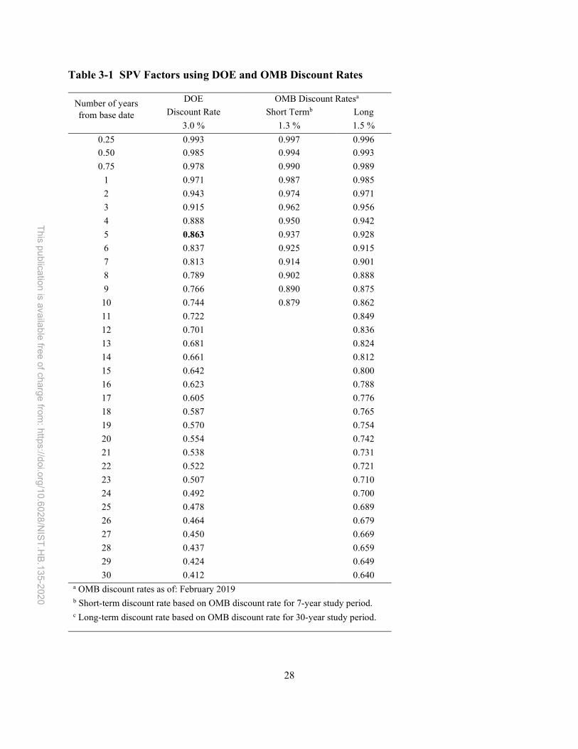
28

This p

ublica

tion is ava

ilab

le free

of ch

arge

from: h

ttps://doi.o

rg/1

0.6

028

/NIS

T.H

B.13

5-202

0

Table 3-1 SPV Factors using DOE and OMB Discount Rates

Number of years from base date

DOE OMB Discount Ratesa

Discount Rate Short Termb Long Termc 3.0 % 1.3 % 1.5 %

0.25 0.993 0.997 0.996

0.50 0.985 0.994 0.993

0.75 0.978 0.990 0.989

1 0.971 0.987 0.985

2 0.943 0.974 0.971

3 0.915 0.962 0.956

4 0.888 0.950 0.942

5 0.863 0.937 0.928

6 0.837 0.925 0.915

7 0.813 0.914 0.901

8 0.789 0.902 0.888

9 0.766 0.890 0.875

10 0.744 0.879 0.862

11 0.722

0.849

12 0.701

0.836

13 0.681

0.824

14 0.661

0.812

15 0.642

0.800

16 0.623

0.788

17 0.605

0.776

18 0.587

0.765

19 0.570

0.754

20 0.554

0.742

21 0.538

0.731

22 0.522

0.721

23 0.507

0.710

24 0.492

0.700

25 0.478

0.689

26 0.464

0.679

27 0.450

0.669

28 0.437

0.659

29 0.424

0.649

30 0.412

0.640 a OMB discount rates as of: February 2019 b Short-term discount rate based on OMB discount rate for 7-year study period. c Long-term discount rate based on OMB discount rate for 30-year study period.

29

This p

ublica

tion is ava

ilab

le free

of ch

arge

from: h

ttps://doi.o

rg/1

0.6

028

/NIS

T.H

B.13

5-202

0

3.2.2 Discounting Annually Recurring Amounts

Annually recurring amounts may be either uniform amounts or non-uniform amounts. Uniform amounts have the same dollar value from year to year, whereas non-uniform amounts change from year to year, either decreasing or increasing at a constant or variable rate.

3.2.2.1 Annually Recurring Uniform Amounts

The uniform present value (UPV) factor, when multiplied by the annually recurring cost, yields the present value of the entire stream of costs over the designated number of years.

Example: An annual maintenance cost of $100 over 5 years, discounted to present value using a 3 % discount rate, yields a present value of $457.97.

𝑃𝑉 = 𝐴0 ∙ (1 + 𝑑)𝑡 − 1

𝑑 ∙ (1 + 𝑑)𝑡= 𝐴0 ∙ 𝑈𝑃𝑉(𝑡,𝑑) = 100 ∙

(1.03)5 − 1

0.03 ∙ (1.03)5= $457.97 (3 − 7)

Table 3-2, a replication of Table A-2 in the Annual Supplement to Handbook 135 (Lavappa & Kneifel, 2019), provides the computed UPV factors for time periods of 1 to 30 years, based on current (2019) discount rates for federal projects. The UPV factor shown in Table 3-2 for 5 years at a 3 % discount rate is 4.580 (in bold), which, when multiplied by the annual amount of $100, yields the same present value as Equation 3-7 (with allowances for rounding), i.e., 𝑃𝑉 = 100 ∙

4.580 = $458.00.

30

This p

ublica

tion is ava

ilab

le free

of ch

arge

from: h

ttps://doi.o

rg/1

0.6

028

/NIS

T.H

B.13

5-202

0

Table 3-2 UPV Factors using DOE and OMB Discount Rates

Number of years from base date

DOE OMB Discount Ratesa

Discount Rate Short Termb Long Termc

3.0 % 1.3 % 1.5 %

1 0.971 0.987 0.985

2 1.913 1.962 1.956

3 2.829 2.924 2.912

4 3.717 3.873 3.854

5 4.580 4.811 4.783

6 5.417 5.736 5.697

7 6.230 6.650 6.598

8 7.020 7.552 7.486

9 7.786 8.442 8.361

10 8.530 9.321 9.222

11 9.253

10.071

12 9.954

10.908

13 10.635

11.732

14 11.296

12.543

15 11.938

13.343

16 12.561

14.131

17 13.166

14.908

18 13.754

15.673

19 14.324

16.426

20 14.877

17.169

21 15.415

17.900

22 15.937

18.621

23 16.444

19.331

24 16.936

20.030

25 17.413

20.720

26 17.877

21.399

27 18.327

22.068

28 18.764

22.727

29 19.188

23.376

30 19.600

24.016 a OMB discount rates as of: February 2019 b Short-term discount rate based on OMB discount rate for 7-year study period. c Long-term discount rate based on OMB discount rate for 30-year study period.

31

This p

ublica

tion is ava

ilab

le free

of ch

arge

from: h

ttps://doi.o

rg/1

0.6

028

/NIS

T.H

B.13

5-202

0

3.2.2.2 Annually Recurring Non-Uniform Amounts

The modified uniform present value (UPV*) factor, can be used to convert to present value a series of annually recurring costs that change from year to year at a constant escalation rate, e, i.e., 𝐴 = 𝐴 ∙ (1 + 𝑒).

Example: A maintenance cost of $100 occurs annually and is expected to increase at 2 % annually over 5 years. When discounted to present value using a discount rate of 3 %, it will yield a present value of $485.62. Note that the annual amount is specified at the price level of the base date when using the UPV or UPV* factors.

𝑃𝑉 = 𝐴 ∙1 + 𝑒

1 + 𝑑= 𝐴 ∙

(1 + 𝑒)

(𝑑 − 𝑒)∙ 1 −

1 + 𝑒

1 + 𝑑= 𝐴 ∙ 𝑈𝑃𝑉( , )

∗

𝑃𝑉 = 𝐴0 ∙(1 + 𝑒)

(𝑑 − 𝑒)∙ 1 −

1 + 𝑒

1 + 𝑑

𝑛

= 𝐴0 ∙ 𝑈𝑃𝑉(𝑡,𝑑)∗ = 100 ∙

(1.02)

(0.01)∙ 1 −

1.02

1.03

5

=

100 ∙ 4.8562 = $485.62 (3 − 8)

The computed UPV* factor for 5 years, at a discount rate of 3 % and a constant escalation rate of 2 %, is 4.8562. UPV* factor tables using current (2019) discount rates (DOE and OMB) for federal projects in combination with constant escalation rates for non-fuel costs are included in the Annual Supplement to Handbook 135 in Table A-3a through Table A-3c. The UPV* factor shown in Table A-3a for 5 years at a 3 % discount rate and 2 % escalation rate is 4.86, which, when multiplied by the annual amount of $100 yields the same present value as Equation 3-7 (with allowances for rounding), i.e., 𝑃𝑉 = 100 ∙ 4.86 = $486.00.

The escalation rates provided in the Annual Supplement to Handbook 135 include increments of 1 % ranging from -5 % to 5%. For the UPV* based on the DOE discount rate, an escalation rate equal to the rate of general inflation is also included. The calculated (implied) inflation rate using the DOE methodology results in a 0.1 % inflation rate in 2019 (see explanation in Section 3.1.2). The FEMP LCC methodology assumes that prices for goods and services other than energy change at approximately the rate of general inflation, so that in a constant dollar analysis the real escalation rate is zero. The use of constant dollars and real escalation rates in FEMP LCC analyses is covered in Section 3.3.

3.2.2.3 Annually Recurring Energy Costs

The FEMP Modified Uniform Present Value (FEMP UPV*) factor is a special UPV* factor for use with annually recurring energy costs. FEMP UPV* factors are pre-calculated, based on the current DOE discount rate and on energy price escalation rates projected by DOE's Energy Information Administration (EIA). The DOE escalation rates vary by year, region (e.g., Northeast Census Region), fuel type (e.g., electricity), and consumer rate type (e.g., industrial). The forecast is based on a mid-range scenario regarding the performance of the domestic

32

This p

ublica

tion is ava

ilab

le free

of ch

arge

from: h

ttps://doi.o

rg/1

0.6

028

/NIS

T.H

B.13

5-202

0

economy and world oil prices over 30 years.3 The FEMP rules in 10 CFR 436 require that these DOE energy price escalation rates be used in LCC analyses of energy and water conservation projects in federal facilities except:

(1) If the federal agency is using actual energy or water prices charged in the base year, that agency may use corresponding escalation rates provided by the energy or water supplier.

(2) For federal buildings in foreign countries, the federal agency may use a “reasonable” escalation rate.

Current FEMP UPV* factors are published in the Annual Supplement to Handbook 135, Table Ba-1 through Table Ba-5 for each of the four major census regions of the United States and the U.S. average. These FEMP UPV* factors, when multiplied by the annual energy cost (as calculated using energy prices as of the base date),4 yield the present value of energy costs for the number of years indicated, given the current DOE discount rate and EIA energy price projects.

Since DOE forecasts of energy price escalation rates vary by fuel (electricity, distillate and residual fuel oils, natural gas, LPG, coal, and gasoline) and rate type (residential, commercial, industrial, and transport), FEMP UPV* factors are computed for each combination of energy type and rate type over study periods ranging from 1 to 30 years.

Example: Assume that you are evaluating an energy conservation project in a federal building located in Connecticut. The annual cost of natural gas for space heating is $20 000, using commercial gas prices as of the beginning of the study period (2019). The present value of these annual gas costs over 20 years can be computed by multiplying the annual cost of $20 000 by the appropriate FEMP UPV* factor of 17.33. The present value is 𝑃𝑉 = 20 000 ∙ 17.33 =

$346 600.

The FEMP UPV* value can be found in Table Ba-1 of the Annual Supplement to Handbook 135, which provides the FEMP UPV* for Census Region 1 for study periods between 1 year and 30 years. The top of the table shows the states located in the census region covered in the table. The FEMP UPV* factor of 17.33 is found in the section headed "Commercial," in the column headed "NtGas," in the row where “N,” the number of years, is 20.

3.2.3 Discounting When There is a Planning/Construction (P/C) Period

For LCC analyses in which a planning/construction (P/C) period occurs before the service date, special consideration must be given to annually recurring costs before discounting them to present value. For one-time costs occurring at any time during the study period, the SPV factor is used as shown above. That is, the present value at the base date is calculated with the appropriate SPV factor for the number of years between the base date and the time the cost is incurred.

3 EIA projections are provided for 25 years with Year 25 through Year 30 being projected using the same escalation rate as Year 25. 4 See Section 4.6 for more details related to the calculation of annual energy costs.

33

This p

ublica

tion is ava

ilab

le free

of ch

arge

from: h

ttps://doi.o

rg/1

0.6

028

/NIS

T.H

B.13

5-202

0

However, this is not the case with annually recurring costs. Annually recurring costs are not generally incurred during the P/C period, but instead are usually assumed to begin at the date the project is put into service. The use of a UPV or UPV* factor based on the full study period, which includes the P/C period, would implicitly include in the present-value calculation annually recurring costs that did not occur in the P/C period. To exclude those costs for the length of the P/C period, take the following steps:

(1) Look up (or calculate) the UPV (UPV*) factor for the number of years in the entire study period (including the P/C period).

(2) Look up (or calculate) the UPV (UPV*) factor for the years in the P/C period. (3) Use the positive difference between the two factors as the appropriate UPV (FEMP UPV*)

factor by which to multiply the annual recurring cost (specified in base-date prices).

This procedure will give the present value as of the base date of the annually recurring costs over only the service period.

Example: Assume that natural gas is to be used in a new heating system in a commercial building in Census Region 1 and is estimated to cost $20 000 annually, based on gas prices at the base date. This system is expected to be put into service three years after the base date and to continue in use for 20 years after the service date.

(1) From Table Ba-1, the FEMP UPV* factor for Census Region 1, commercial natural gas, for 23 years (3 years P/C period plus 20 years of usage), is 19.26.

(2) The corresponding FEMP UPV* factor for 3 years (the P/C period) is 2.93. (3) The difference between these two factors (19.26 – 2.93 = 16.33) is the appropriate FEMP

UPV* factor for computing the present value of the natural gas usage over 20 years as of the base date.

Multiplying the $20 000 annual natural gas costs by the FEMP UPV* (16.33) generates a present value of $326 600.

3.3 Adjusting for Inflation

Inflation reduces the purchasing power of the dollar over time; deflation increases it. When future amounts are stated in prices as of the year in which they are expected to occur, they are said to be in current dollars. Current dollars are dollars of any one year's purchasing power, inclusive of inflation. That is, they reflect changes in the purchasing power of the dollar from year to year. In contrast, constant dollars are dollars of uniform purchasing power, exclusive of inflation. Constant dollars indicate what the same good or service would cost at different times if there were no change in the general price level – no inflation or deflation – to change the purchasing power of the dollar.

To make a meaningful comparison between costs occurring at different points in time, those costs must be adjusted for changes in the purchasing power of the dollar. To measure costs with inflated or deflated dollars is meaningless, just as it would be meaningless to measure a

34

This p

ublica

tion is ava

ilab

le free

of ch

arge

from: h

ttps://doi.o

rg/1

0.6

028

/NIS

T.H

B.13

5-202

0

building's dimensions with an elastic tape measure. The adjustment of costs from current to constant dollars is not the same as discounting future costs to present value. The former adjusts only for changes in the purchasing power of the dollar; the latter adjusts for an individual investor's time-value of money. The appropriate discount rate needed to adjust future costs to their present value will be different depending on whether future costs are stated in constant dollars or current dollars. Even when costs are expressed in constant dollars, the discount rate is usually positive, reflecting the real earning power of money over and above the general rate of inflation.

3.3.1 Two Approaches for Dealing with Inflation

The FEMP methodology for LCC analysis allows cash flows to be stated either in constant dollars or current dollars. However, the constant dollar method is preferred and is the methodology supported by Handbook 135 and the Annual Supplement to Handbook 135.

The constant dollar approach has the advantage of avoiding the need to project future rates of inflation or deflation. The price of a good or service stated in constant dollars is not affected by the rate of general inflation. For example, if the price of a piece of equipment is $1000 today and $1050 at the end of a year in which prices in general have risen at an annual rate of 5 %, the price stated in constant dollars is still $1000. If cash flows are stated in current dollars, future amounts include general inflation, and an adjustment is necessary to convert the current-dollar estimate to its constant-dollar equivalent. This adjustment is important because constant- and current-dollar amounts must not be combined in an LCCA.

There are two ways to arrive at constant dollar amounts in an LCCA. Both methods need to be looked at in combination with the discount rate.

Method 1: Estimate future costs and savings in constant dollars and discount with a "real" discount rate, i.e., a discount rate that excludes the rate of inflation, or

Method 2: Estimate future costs and savings in current dollars and discount with a "nominal" discount rate, i.e., a discount rate that includes the rate of inflation.

Both approaches will yield the same present value results, and thus support the same conclusion, provided consistent assumptions are made about the real discount rate and the rate of inflation. However, it is generally easier to conduct an economic analysis in constant dollars because the rate of inflation from year to year over the study period need not be estimated. The analyst chooses a reference date for fixing the value of the dollar and expresses all future amounts in dollars of the same value, for example, in constant 2018 dollars. The reference date is usually chosen to coincide with the beginning of the study period, since that year’s dollar costs (for expenses expected to occur during the study period) are usually known, but it could be any date.

It is important in this context to distinguish between a present value analysis, where future costs are adjusted to time-equivalent values, and a budget analysis, where funds must be appropriated for year-to-year disbursements. The purpose of a present value analysis is to determine whether

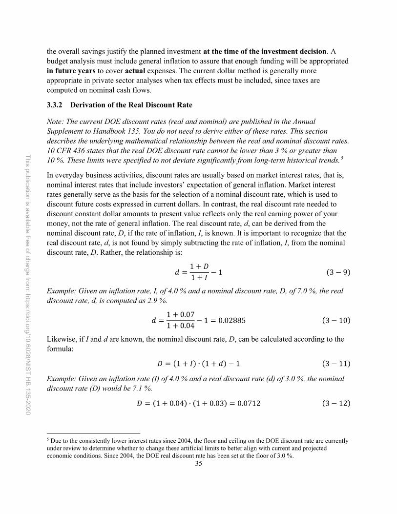
35

This p

ublica

tion is ava

ilab

le free

of ch

arge

from: h

ttps://doi.o

rg/1

0.6

028

/NIS

T.H

B.13

5-202

0

the overall savings justify the planned investment at the time of the investment decision. A budget analysis must include general inflation to assure that enough funding will be appropriated in future years to cover actual expenses. The current dollar method is generally more appropriate in private sector analyses when tax effects must be included, since taxes are computed on nominal cash flows.

3.3.2 Derivation of the Real Discount Rate

Note: The current DOE discount rates (real and nominal) are published in the Annual Supplement to Handbook 135. You do not need to derive either of these rates. This section describes the underlying mathematical relationship between the real and nominal discount rates. 10 CFR 436 states that the real DOE discount rate cannot be lower than 3 % or greater than 10 %. These limits were specified to not deviate significantly from long-term historical trends.5

In everyday business activities, discount rates are usually based on market interest rates, that is, nominal interest rates that include investors’ expectation of general inflation. Market interest rates generally serve as the basis for the selection of a nominal discount rate, which is used to discount future costs expressed in current dollars. In contrast, the real discount rate needed to discount constant dollar amounts to present value reflects only the real earning power of your money, not the rate of general inflation. The real discount rate, d, can be derived from the nominal discount rate, D, if the rate of inflation, I, is known. It is important to recognize that the real discount rate, d, is not found by simply subtracting the rate of inflation, I, from the nominal discount rate, D. Rather, the relationship is:

𝑑 =1 + 𝐷

1 + 𝐼− 1 (3 − 9)

Example: Given an inflation rate, I, of 4.0 % and a nominal discount rate, D, of 7.0 %, the real discount rate, d, is computed as 2.9 %.

𝑑 =1 + 0.07

1 + 0.04− 1 = 0.02885 (3 − 10)

Likewise, if I and d are known, the nominal discount rate, D, can be calculated according to the formula:

𝐷 = (1 + 𝐼) ∙ (1 + 𝑑) − 1 (3 − 11)

Example: Given an inflation rate (I) of 4.0 % and a real discount rate (d) of 3.0 %, the nominal discount rate (D) would be 7.1 %.

𝐷 = (1 + 0.04) ∙ (1 + 0.03) = 0.0712 (3 − 12)

5 Due to the consistently lower interest rates since 2004, the floor and ceiling on the DOE discount rate are currently under review to determine whether to change these artificial limits to better align with current and projected economic conditions. Since 2004, the DOE real discount rate has been set at the floor of 3.0 %.

36

This p

ublica

tion is ava

ilab

le free

of ch

arge

from: h

ttps://doi.o

rg/1

0.6

028

/NIS

T.H

B.13

5-202

0

For a rough estimate of real or nominal discount rates, it is acceptable to subtract or add the rate of inflation, but to assure that the results of an economic evaluation are the same no matter whether cash flows are stated in current or in constant dollars, the rates need to be computed according to the above formulas.

3.3.3 Price Escalation

Few commodities have prices that change at exactly the rate of general inflation (that is, the rate of change in the price level of all items) year after year, but many commodities have prices that change at a rate close to that of general inflation over time. Figure 3-2 shows, for 2008 through 2017, the rate of general inflation and the rates of (nominal) price escalation for several commodities related to buildings: maintenance and repair costs, construction material and supplies dealers, natural gas, and fuel oil.

Figure 3-2 Rate of Price Changes for Home-Related Items Compared with "All Items"

As is evident from Figure 3-2, only for fuel oil and natural gas have price escalation rates deviated substantially from the rate of general inflation over most of these years. Rates of price change for the other building-related items shown (Building Material and Supplies Dealers and Non-residential Building M&R) have generally tracked the rate of change in the general price level with the total inflation rate from 2010 through 2017 within 1.0 percentage point, so that the relative price change for these items is zero. For this reason, the FEMP LCC methodology, which recommends that future costs be expressed in constant dollars, generally assumes a zero

37

This p

ublica

tion is ava

ilab

le free

of ch

arge

from: h

ttps://doi.o

rg/1

0.6

028

/NIS

T.H

B.13

5-202

0

real (differential) escalation rate for all non-energy related costs. DoD provides its own best practices on inflation and escalation estimation in DoD (2017b).

3.3.3.1 Nominal Price Escalation

To estimate the actual (nominal) cost of a particular commodity as of some future date, Ct, where t is the number of time periods between the base date and the date that the cost is incurred, the cost of that commodity as of the base date, C0, must be adjusted to reflect the nominal price escalation rate, E, for that commodity over the t time periods, using the following formula:

𝐶 = 𝐶 ∙ (1 + 𝐸) (3 − 13)

Example: A replacement costing $1000 today that escalates at a nominal rate of 3 % annually will cost approximately $1344 ten years from now.

𝐶 = 1000 ∙ (1 + 0.03) = $1344 (3 − 14)

The nominal rate of price escalation, E, may be, but is not necessarily, the same as the rate of general inflation, I, which represents the rate of increase in prices for all goods and services.6

3.3.3.2 Real Price Escalation

If the nominal rate of price escalation, E, for a commodity is different from the general rate of inflation, then a real (differential) rate of escalation, e, should be computed using the following formula:

𝑒 =1 + 𝐸

1 + 𝐼− 1 (𝟑 − 15)

For example, given an inflation rate, I, of 4.0 % and a nominal escalation rate, E, of 5.0 %, the real escalation rate, e, is computed as 0.96 %.

𝑒 =1 + 0.05

1 + 0.04− 1 = 0.009615 (𝟑 − 16)

Or, given the real escalation rate, the nominal escalation rate can be computed as

𝐸 = (1 + 𝐼) ∙ (1 + 𝑒) − 1 (𝟑 − 17)

For example, given an inflation rate of 4.0 % and a real escalation rate of 2.0 %, the nominal escalation rate would be 6.1 %.

𝐸 = (1 + 0.04) ∙ (1 + 0.02) − 1 = 0.06080 (𝟑 − 17)

6 Just as the rate of general inflation (I) may not be constant from year to year (E) may not be constant from year to year. When E is not constant from year to year, the cost of a commodity in year t must be calculated by compounding the annual escalation rates as follows: 𝐶 = 𝐶 ∙ (1 + 𝐸 ) ∙ (1 + 𝐸 ) ∙ (1 + 𝐸 ) ∙ … ∙ (1 + 𝐸 )

38

This p

ublica

tion is ava

ilab

le free

of ch

arge

from: h

ttps://doi.o

rg/1

0.6

028

/NIS

T.H

B.13

5-202

0

Just as the real discount rate, d, is not the difference between the nominal discount rate, D, and the rate of general inflation, I, the real escalation rate, e, for a commodity is not the difference between the nominal escalation rate, E, and the rate of general inflation, I.

In order to estimate the cost, Ct, of a commodity in constant base-year dollars as of some future point in time t, where t is the number of time periods between the base date and the date that the cost is incurred, the cost of that commodity today, C0, must be adjusted to reflect the real price escalation rate, e, for that commodity over the t time periods, using the following formula:

𝐶 = 𝐶 ∙ (1 + 𝑒) (3 − 18)

Example: A replacement cost of $1000 today, which escalates at a real rate of 1 % annually (i.e., 1 % greater than the general inflation rate), will cost approximately $1105 ten years from now, in base-year constant dollars.

𝐶 = 1000 ∙ (1 + 0.01) = $1105 (3 − 19)

If the replacement cost decreases in real terms (i.e., its nominal escalation rate is less than the rate of general inflation), then its future cost in constant base-year dollars will be less than its cost as of the base date.

Example: If in the previous example, the real escalation rate is assumed to be -1 % (i.e., 1 % less than the general inflation rate), then that cost would be approximately $904 ten years later, in constant base-year dollars.

𝐶 = 1000 ∙ (1 − 0.01) = $904 (3 − 20)

Table 3-3 summarizes the formulas used to calculate the real and nominal discount rates and escalation rates needed to adjust LCC cash flows for the underlying inflation rate (I).

Table 3-3 Summary of Inflation-Adjustment Formulas

Nominal Discount Rate: D = (1 + 𝑑) ∙ (1 + 𝐼) − 1

Real Discount Rate: d = (1 + 𝐷)/(1 + 𝐼) − 1

Nominal Escalation Rate: E = (1 + 𝑒) ∙ (1 + 𝐼) − 1

Real Escalation Rate: e = (1 + 𝐸)/(1 + 𝐼) − 1

3.3.4 Real Escalation of Energy-Related Cash Flows

For energy-related costs, the FEMP LCC methodology requires the use of DOE-projected real escalation rates by fuel type, rate type, and census region, as published in the Annual Supplement to Handbook 135 for domestically located facilities unless actual prices in the base year and projections from the servicing utility are available. The FEMP UPV* factors published in that supplement, which incorporate these escalation rates, are automatically applied in an LCCA that

39

This p

ublica

tion is ava

ilab

le free

of ch

arge

from: h

ttps://doi.o

rg/1

0.6

028

/NIS

T.H

B.13

5-202

0

is performed using the NIST BLCC computer programs. However, 10 CFR 436 does permit the use of alternative real escalation rates for a FEMP LCCA for those years for which the local energy supplier can provide a firm estimate of the anticipated rate of price increase. In such a case, the computation of the appropriate UPV* factor is more complex and should generally be performed using the NIST BLCC computer program or software consistent with this program.

Coleman (2015) considered the impact of over- and under-estimation of energy price escalation rates on the cost savings from ESPC projects. The study found that the escalation rates developed by NIST for the Annual Supplement to Handbook 135 and implemented in associated NIST software (EERC and BLCC) can be considered reasonable and defensible but have generally represented lower-end estimates. The study found that since 2000 EIA energy price estimates have had a downward bias relative to actual realized prices. Under-estimating escalation rates ensures that realized energy cost savings will be greater than projected energy cost savings, and therefore greater than the ESPC payments. However, due to this trend of inherent conservatism from EIA, escalation rates lower than those developed by NIST with the EIA data should not be used because they can lead to either under-investment (i.e., cost-effective energy conservation measures (ECMs) not adopted) and/or longer-term contracts (due to lower annual payments) that will result in greater overall project costs.

3.3.5 Illustration of Discounting Constant-Dollar and Current-Dollar Cash Flows

Use a real discount rate, d,

if you express cash flows in constant dollars, including only the differential rate of price escalation;

Use a nominal discount rate, D,

if you express cash flows in current dollars, including both the differential rate of price escalation and general inflation.

The following example shows that both approaches result in the same present value and thus support the same decision.

Example: Suppose you want to know the present value of an air-conditioning compressor that you expect to replace in 15 years. If the AC compressor were replaced today, the price would be $5000. Due to advanced manufacturing processes, you expect that the price of compressors will increase at a rate of 2 % lower than general price inflation. You estimate the rate of general price inflation to be 5 % annually. You know that your real discount rate is 3 %.

To summarize:

I = 0.05 t = 15 years

d = 0.03 D = (1 + 0.03) ∙ (1 + 0.05) − 1 = 0.0815

e = -0.02 E = (1 − 0.02) ∙ (1 + 0.05) − 1 = 0.0290

40

This p

ublica

tion is ava

ilab

le free

of ch

arge

from: h

ttps://doi.o

rg/1

0.6

028

/NIS

T.H

B.13

5-202

0

Constant Dollars and Real Discount Rate

Current Dollars and Nominal Discount Rate

𝑃𝑉 = 𝐹 ∙1 + 𝑒

1 + 𝑑 PV = 𝐹 ∙

1 + 𝐸

1 + 𝐷

= 5000 ∙1 − 0.02

1 + 0.03 = 5000 ∙

1 − 0.0290

1 + 0.0815

= 5000 ∙ 0.4741 = 5000 ∙ 0.4741

= $2370.30 = $2370.30

41

This p

ublica

tion is ava

ilab

le free

of ch

arge

from: h

ttps://doi.o

rg/1

0.6

028

/NIS

T.H

B.13

5-202

0

42

This p

ublica

tion is ava

ilab

le free

of ch

arge

from: h

ttps://doi.o

rg/1

0.6

028

/NIS

T.H

B.13

5-202

0

4 Estimating Costs for LCCA

This chapter provides details on identifying the type and timing of each potential cost or benefit for a project, and estimation guidance dependent on these factors.

4.1 Relevant Effects

There are numerous costs associated with acquiring, operating, maintaining, and disposing of a facility, system, or even individual piece of equipment. Which of these costs needs to be included is one of the first decisions to be made when performing an LCCA of alternative energy efficiency, water conservation, or renewable energy strategies. To answer this question, it is necessary to look at the economic effects that will result from each design alternative. To the extent feasible, these effects need to be quantified in dollar terms. For effects that cannot be expressed as dollar amounts, either an alternative non-monetary metric (quantitative) or a descriptive account (qualitative) should be given so that they can be included in the analysis. These additional effects are particularly important for whole building, facility, or campus-wide projects because of the broad interactions across systems and resulting (potentially significant) direct and indirect effects. See Section 9.4 for additional information on whole building LCCA.

It is not necessary to include all project-related costs in an LCCA of project alternatives. Only those costs that are relevant to the decision and significant in amount are needed to make a valid investment decision. Costs are relevant to the decision when they change from alternative to alternative. Costs that are approximately the same for each alternative will not be a determining factor in the choice among the alternatives and, therefore, can be omitted from the LCC calculation. Inclusion of such costs will not produce erroneous results but may incur data collection and analysis costs that could be avoided. Costs are significant when they are large enough to make a credible difference in the LCC of a project alternative. Energy costs, for example, are likely to be relevant and significant in the analysis of alternative window designs for an office building but not in the analysis of low-flow bathroom fixtures. Assessing the relevance and significance of project costs in an LCCA is largely a matter of analyst judgment. However, guidance provided by FEMP and other federal agencies can assist in identifying which effects and associated metrics and data sources should be considered and/or included in a LCCA.

Sunk costs should be excluded from an LCCA. These are costs that have been incurred or committed to in the past and thus cannot be avoided by a future decision. For example, the cost of a recently replaced fuel tank for an oil heating system being converted to natural gas is a sunk cost (except for any associated salvage value).

In the LCCA of direct-funded federal energy efficiency, water conservation, and renewable energy projects, tax effects and finance costs (i.e., interest charges) are generally not relevant and can be omitted from the LCCA. However, when evaluating alternative methods of funding these projects for federal facilities (e.g., appropriations funding versus financed options (e.g., energy savings performance contracts or utility energy service contracts)), the relative cost-effectiveness of the projects under each of these funding alternatives should be evaluated from an LCC

43

This p

ublica

tion is ava

ilab

le free

of ch

arge

from: h

ttps://doi.o

rg/1

0.6

028

/NIS

T.H

B.13

5-202

0

perspective before deciding which method(s) of funding are most advantageous to the federal government. (This subject is discussed further in Chapter 10.)

Developing cost estimates can be completed using numerous methods, whether its applying quotes received directly from a contractor, using an average from multiple industry cost databases, or extrapolating existing costs using current prices and future projections. Chapter 11 of GAO (2009b) provides guidance on developing a point estimate, with an overview of different cost estimating methods focused on analogy, engineering build-up, and parametric methods while also discussing expert opinion, extrapolation, and learning curves. The appropriate method or combination of methods will depend on the specific cost being estimated and available information available. This chapter will provide structure, resources, and guidance on estimating costs. The analyst should exercise their best judgement for each cost estimate and clearly document those decisions.

4.2 Cost Categories

There are various ways of classifying the cost components of an LCCA, depending on what role they play in the mechanics of the methodology. The most important categories in LCCA distinguish between investment-related and operational costs; initial and future costs; and single versus annually recurring costs.

4.2.1 Investment Costs vs. Operational Costs

Life-cycle costs typically include both investment costs and operational costs. The distinction between investment and operation-related (all non-investment) costs is most useful when computing supplementary economic measures such as the savings-to-investment ratio (SIR) and adjusted internal rate of return (AIRR). These measures evaluate savings in operations-related costs with respect to increases in capital investment costs. This distinction will not affect the LCC calculation itself, nor will it cause a project alternative to change from cost-effective to non-cost effective or vice versa. However, it may change its ranking relative to other independent projects when allocating a limited capital investment budget. (Supplementary measures are discussed in Chapter 6 while budget allocation methods are discussed in Section 7.5.)

All acquisition costs, including costs related to planning, design, purchase, and construction, are initial investment-related costs. The FEMP LCC methodology in 10 CFR 436 also requires that residual values (resale value, salvage value, or disposal costs) and capital replacement costs be included as future investment-related costs. Capital replacement costs are usually incurred when replacing major systems or components, paid from capital funds. Residual values are negative investment costs that are recovered at the end of the study period.

Operating, maintenance, and repair (OM&R) costs, including energy and water costs, are operational costs. Replacements that are related to maintenance or repair (e.g., replacing light bulbs or a circuit board) are usually considered to be OM&R costs, not capital replacement costs. OM&R costs are usually paid from an annual operating budget instead of capital funds.

44

This p

ublica

tion is ava

ilab

le free

of ch

arge

from: h

ttps://doi.o

rg/1

0.6

028

/NIS

T.H

B.13

5-202

0

4.2.2 Initial Investment Costs vs. Future Costs

The distinction between initial investment costs and future costs is most useful when computing the simple or discounted payback measures. The costs incurred in the planning, design, construction and/or acquisition phase of a project are classified as initial investment costs. They usually occur before a building is occupied or a system is put into service. Those costs that arise from the operation, maintenance, repair, replacement, and use of a facility or a system during its occupancy or service period are future costs. Residual values at the end of a system life, or at the end of the study period, are also future costs.

4.2.3 Single Costs vs. Annually Recurring Costs

It is useful to establish two categories of project-related costs based on their frequency of occurrence. This categorization determines the type of present value factor to be used for discounting future cash flows.

(1) Single costs (one-time costs) occur at one or more times during the study period at irregular or non-annual intervals. Initial investment costs, replacement costs, residual values, maintenance costs scheduled at intervals longer than one year, and repair costs are usually treated as single costs. The SPV factor is the appropriate present value factor for single costs.

(2) Annually recurring costs are amounts that occur regularly every year during the service period in approximately the same amount, or in an amount expected to change at some known rate. Energy costs, water costs, and routine annual maintenance costs fall into this category. The appropriate present value factor for annually recurring amounts is the UPV factor or UPV* factor. If recurring costs are the same each year, the UPV factor is the appropriate present value factor. If the annual amounts are expected to change at a known rate, the UPV* factor is the appropriate present value factor.

4.3 Timing of Cash Flows

LCCA requires that all project-related costs be identified by time of occurrence as well as amount. However, it is a well-accepted convention in LCCA to use simplifying models of cash flows rather than to attempt to reproduce the exact timing of all costs. Thus, costs that occur at different times during the year can all be treated as occurring at the same time each year to simplify the discounting operations. LCCA software makes it more convenient to compute single costs from their actual time of occurrence during the year.

4.3.1 Federal Cash-Flow Conventions

FEMP LCC rules (10 CFR 436) allow both single and annually recurring costs to be discounted either from the actual time of occurrence or from the end of the year in which they occur. The FEMP convention (as reflected historically in Handbook 135 and the discount factor tables in the Annual Supplement to Handbook 135) has been to discount all costs from the end of the year in

45

This p

ublica

tion is ava

ilab

le free

of ch

arge

from: h

ttps://doi.o

rg/1

0.6

028

/NIS

T.H

B.13

5-202

0

which they occur. However, since LCC software (e.g., BLCC) is now used for most LCC computations, other cash flow conventions are often implemented. The most appropriate cash flow handling for any given cost category varies with the complexity of the analysis, the computational basis (manual versus computer), and specific customer requirements.

When using manual methods, it’s typically sufficient to discount all costs from the end of the year in which they occur. The present value tables provided in the Annual Supplement to Handbook 135 are based on this end-of-year discounting convention. With software-based analysis, the recommended method is to discount all single costs from the time of occurrence and to discount annually recurring costs from the end of each service year (consistent with the UPV or UPV* factors shown in this handbook). However, for military construction projects in the U.S. Department of Defense (subject to the Tri-Services Memorandum of Agreement (Tri-Services, 1991)), initial investment costs are usually discounted from the mid-point of construction, and annually recurring OM&R costs (including energy and water costs) are discounted from the mid-point of each service year.

4.3.2 Cash-Flow Diagrams

A cash-flow diagram for a project alternative, as shown in Figure 4-1, provides a convenient way of visualizing all relevant costs and their timing. A horizontal timeline represents the study period and marks each year and key dates (e.g., the base date, the occupancy or service date, and the end of the study period). Years can be marked in calendar-year terms (e.g., 2018) or in elapsed years from the base date (e.g., 1, 2, 3, ...). There is no standard convention for showing costs on a cash flow diagram, but positive costs are typically shown above the horizontal timeline, and negative costs (e.g., residual values) are shown below the timeline. The cash flow diagram for Project "A" in Figure 4-1 shows a study period of 15 years, from January 2018 through December of 2032. An initial investment of $5000 is shown at the base date, with a residual value of $200 at the end of the study period. Annually recurring OM&R costs of $600 (in base-date dollars) are shown, along with a one-time OM&R cost of $400 in 2022.

46

This p

ublica

tion is ava

ilab

le free

of ch

arge

from: h

ttps://doi.o

rg/1

0.6

028

/NIS

T.H

B.13

5-202

0

Figure 4-1 Cash Flow Diagram

4.4 Using Base-Date Prices to Estimate Future Costs

Most cost data for an LCCA are likely to be estimates. The analysis is often performed early in the decision-making process before detailed initial cost data are available, and future costs by their nature are uncertain. The difficult task of obtaining estimates of future costs is simplified by in the FEMP LCC methodology by allowing future cost estimates to be based on their corresponding cost as of the base date of the LCCA, usually the date on which the analysis is performed.

If there is reason to believe that the supply and demand conditions for a good or service remain the same as those for most other goods and services, it can be assumed that its price will change at roughly the rate of general price inflation. That is, the real price escalation rate is equal to zero. This means that in a constant dollar analysis - where the rate of inflation is not included in the computations - the future price of an item is identical to the base-date price. One of the basic assumptions of the FEMP LCC methodology is that prices for all goods and services, other than for energy and water, will increase at approximately the same rate as general inflation. However, if there is a documentable basis for assuming that prices change at a rate different than general inflation (for example, when price escalation rates are established in a maintenance contract), these rates can be used in the analysis.

Section 3.3.3 provides the methodology used to convert prices (or costs) at the base date to prices (or costs) at a future date when appropriate price escalation rates are available. However, this step is not usually required for energy costs in an LCCA because the present value factors provided in the annual supplement to this handbook account for real price escalation rates. (See Section 3.2.2.2 for information on discounting non-uniform annual amounts.)

Even in the case of energy and water prices, the base-date price is used as the basis for estimating future prices in the FEMP LCC methodology. Tools like NIST/DOE’s EERC, which is predicated on DOE-EIA’s energy price projections, provide price escalation rates for use in estimating future energy prices, but these are used with local energy price schedules as of the

$400

$600 $600 $600 $600 $600 $600 $600 $600 $600 … $600

$5000

Year 2018 2019 2020 2021 2022 2023 2024 2025 2026 … 2032

Base Date Service Date

$200 End of

Study Period

47

This p

ublica

tion is ava

ilab

le free

of ch

arge

from: h

ttps://doi.o

rg/1

0.6

028

/NIS

T.H

B.13

5-202

0

base date. NIST/DOE does not provide price escalation rates for water because these rates are very sensitive to existing and projected infrastructure conditions at the community level.

4.5 Estimating Investment-Related Costs

Investment costs include initial project costs, future capital replacement costs, and the residual value of these investments at the end of the study period. This section will provide details on how to estimate investment-related costs.

4.5.1 Estimating Initial Investment Costs

Initial investment costs are probably the least difficult project costs to estimate because they occur relatively close to the present time. Quotes for purchase and installation costs can often be obtained from local suppliers or contractors. You can also develop estimates by adding unit costs obtained from construction cost-estimating guides, for which a (non-complete) list is provided in Table 4-1. They are published as tables, usually in electronic form.

Since the estimates are based on different underlying assumptions and have different emphases, we recommend that you use the same data set for analyzing each of the alternatives being considered for a project to get consistent and comparable results.

48

This p

ublica

tion is ava

ilab

le free

of ch

arge

from: h

ttps://doi.o

rg/1

0.6

028

/NIS

T.H

B.13

5-202

0

Table 4-1 Suggested Cost-Estimating Resources for LCCA of Buildings

Resource Source Description RSMeans https://www.rsmeansonline.com/ new construction, repair and

remodeling, facilities maintenance, and green building cost library

Grainger Industrial

https://www.grainger.com/ wholesaler of construction materials

CBRE CostLab

https://www.cbre.com/real-estate-services/occupier/client-strategy-and-consulting/cbre-business-analytics/costlab

facility benchmarking, budgeting, and capital planning

GSA Advantage

https://www.gsaadvantage.gov/advantage /main/home.do GSA-provided purchasing portal for federal agencies to acquire commercial products and services

D4COST http://www.d4cost.com/ building cost estimating software for conceptual estimating created from actual projects

BNi Building NEws

https://www.bnibooks.com/ Reference Construction Cost Books based on costs from actual projects

Craftsman https://www.craftsman-book.com/ Single family cost and appraisal estimate resources

Urban Land Institute (dated)

https://uli.bookstore.ipgbook.com/dollars---cents-of-shopping-centers---the-score---2008-products-9780874200959.php?page_id=32&pid=ULI

data tables on income and expenses for all types, sizes, and ages of shopping centers and their tenants

CALIBRE (originally ERDC)

https://www.calibresys.com/documents/service/ BUILDER_Sustainment%20Management.pdf

Builder Sustainment Management Services (SMS)

Marshall & Swift (CoreLogic)

https://www.corelogic.com/solutions/marshall-swift.aspx Building cost data provided based on building area, assembly, and unit.

BOMA EER https://eer.boma.org/BOMA/main_landing.aspx Detailed income, expense and occupancy information for office and industrial sectors

Richardson Engineering Database

https://www.eosgroup.com/products/knowledgebases/richardson-engineering

Process plant construction (material, equipment, labor) cost data

Note: Most of the listed publishers issue additional, more specialized, cost guides

Detailed estimates of construction costs are not necessary for preliminary economic analyses of alternative facility designs or systems. Such estimates are usually not available until the design is quite advanced and the opportunity for cost-reducing design changes has been missed. For very large projects you may want to use a standard format for organizing construction cost data to facilitate the retrieval and review of the data. UNIFORMAT II (Charette & Marshall, 1999), which has been published as a standard classification scheme by ASTM (ASTM, 2015e),

49

This p

ublica

tion is ava

ilab

le free

of ch

arge

from: h

ttps://doi.o

rg/1

0.6

028

/NIS

T.H

B.13

5-202

0

organizes costs into three levels for each of 12 work categories (e.g., category 03, superstructure; category 06, interior construction; and category 12, site work). The hierarchical system allows for cost estimates at a broader level at the beginning of the project and at a more detailed level as the design of the project progresses.

4.5.2 Estimating Capital Replacement Costs

The number and timing of capital replacements depends on the estimated life of the system and the length of the service period. You can use the same sources that provide cost estimates for initial investments to obtain estimates of replacement costs and expected lives. A good starting point for estimating future replacement costs is to use their cost as of the base date. In a FEMP LCCA conducted in constant dollars with real price escalation rates equal to zero, the future cost will be the same as the base-date cost. When a non-zero real price escalation rate is appropriate, consult Section 3.3.3 to see how to compute future replacement costs and present values.

4.5.3 Estimating Residual Values

The residual value of a system (or component) is its remaining value at the end of the study period, or at the time that it is replaced during the study period. Residual values can be based on value in place, resale value, salvage value, or scrap value, net of any selling, conversion, or disposal costs.

The residual value of a system at the end of its expected useful life is likely to be small or even negative (due to removal or disposal costs) if the system needs complete replacement or the facility is being demolished. However, for systems with expected lives extending beyond the end of the study period, the residual value should be based on their value in place, not on their "salvage" value as if they were to be removed from the building at that point. A facility system that is functioning in place adds significant value to the building and this value should be reflected in its residual value. There are numerous methods in estimating this value that may be appropriate depending on the application. It is recommended that you consider values that can be quantified using market-based data.

Building appraisers use numerous approaches in valuing building improvements. The simplest and most traditional approach for federal facilities is to estimate the residual value of a system with remaining useful life by linearly prorating (depreciation) its initial cost. For example, assume an on-site solar photovoltaic system (10 kW) with a capital investment cost of $30 000 is expected to have a service life of 25 years while the study period of interest is 15 years. The

residual value would be approximately = of its initial cost. Assuming a 3 % discount

rate, the present value of the residual value is $30 000 ∙ ∙ ( . )

= $5731.

A common approach for projects that lower operational costs is to estimate the present value of future cost savings for all years after the end of the study period. For example, assume the same project generates 12 000 kWh of electricity worth $1200 annually ($0.10/kWh) with no real

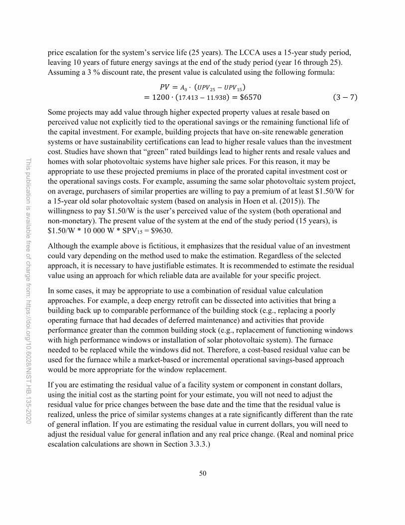
50

This p

ublica

tion is ava

ilab

le free

of ch

arge

from: h

ttps://doi.o

rg/1

0.6

028

/NIS

T.H

B.13

5-202

0

price escalation for the system’s service life (25 years). The LCCA uses a 15-year study period, leaving 10 years of future energy savings at the end of the study period (year 16 through 25). Assuming a 3 % discount rate, the present value is calculated using the following formula:

𝑃𝑉 = 𝐴0 ∙ (𝑈𝑃𝑉25 − 𝑈𝑃𝑉15)

= 1200 ∙ (17.413 − 11.938) = $6570 (3 − 7)

Some projects may add value through higher expected property values at resale based on perceived value not explicitly tied to the operational savings or the remaining functional life of the capital investment. For example, building projects that have on-site renewable generation systems or have sustainability certifications can lead to higher resale values than the investment cost. Studies have shown that “green” rated buildings lead to higher rents and resale values and homes with solar photovoltaic systems have higher sale prices. For this reason, it may be appropriate to use these projected premiums in place of the prorated capital investment cost or the operational savings costs. For example, assuming the same solar photovoltaic system project, on average, purchasers of similar properties are willing to pay a premium of at least $1.50/W for a 15-year old solar photovoltaic system (based on analysis in Hoen et al. (2015)). The willingness to pay $1.50/W is the user’s perceived value of the system (both operational and non-monetary). The present value of the system at the end of the study period (15 years), is $1.50/W * 10 000 W * SPV15 = $9630.

Although the example above is fictitious, it emphasizes that the residual value of an investment could vary depending on the method used to make the estimation. Regardless of the selected approach, it is necessary to have justifiable estimates. It is recommended to estimate the residual value using an approach for which reliable data are available for your specific project.

In some cases, it may be appropriate to use a combination of residual value calculation approaches. For example, a deep energy retrofit can be dissected into activities that bring a building back up to comparable performance of the building stock (e.g., replacing a poorly operating furnace that had decades of deferred maintenance) and activities that provide performance greater than the common building stock (e.g., replacement of functioning windows with high performance windows or installation of solar photovoltaic system). The furnace needed to be replaced while the windows did not. Therefore, a cost-based residual value can be used for the furnace while a market-based or incremental operational savings-based approach would be more appropriate for the window replacement.

If you are estimating the residual value of a facility system or component in constant dollars, using the initial cost as the starting point for your estimate, you will not need to adjust the residual value for price changes between the base date and the time that the residual value is realized, unless the price of similar systems changes at a rate significantly different than the rate of general inflation. If you are estimating the residual value in current dollars, you will need to adjust the residual value for general inflation and any real price change. (Real and nominal price escalation calculations are shown in Section 3.3.3.)

51

This p

ublica

tion is ava

ilab

le free

of ch

arge

from: h

ttps://doi.o

rg/1

0.6

028

/NIS

T.H

B.13

5-202

0

When the study period is very long, the residual value of the original system may be small and largely offset by disposal costs. Discounting further diminishes its weight in the analysis, and so it may be less important to improve the estimate of a residual value than of other input values. But when the study period is short relative to the service life, the estimate of the residual value may become a critical factor in assessing the cost-effectiveness of a capital investment project, and thus it should be given careful consideration. The residual value estimate for a capital replacement, needed to extend the life of an alternative to the length of a common study period, may also be a critical factor in the LCCA and thus care should be given in estimating this value.

Figure 4-2 and Figure 4-3 illustrate the concept of residual value (assuming a linear depreciation method) for new building construction (with and without regular maintenance) and building retrofit, respectively, at two levels of performance. Higher initial investment costs and/or market value of the high-performance building lead to higher residual values (Added Value) throughout the study period relative to a standard building design as shown in Figure 4-2. Note that the building service life is assumed the same for both building designs with regular maintenance, which leads to different slopes for the residual value as both buildings depreciate to zero in the same year. Additionally, the residual value of the standard building design is compared across two scenarios: regular maintenance and deferred maintenance. In the case of deferred maintenance, the residual value decreases at a faster rate because the equipment deteriorates faster, leading to a shorter equipment service life and more frequent replacements. This illustrates how lower O&M costs from deferring maintenance can lead to other, potentially higher costs in equipment replacements and lost residual value. Note that the projected performance deterioration could be non-linear, both for systems that have regular maintenance as well as those with deferred maintenance. See Chapter 14 for a visual example.

Figure 4-2 Building Value – New Construction

0 5 10 15 20 25 30 35 40

Bui

ldin

g V

alue

Building LifeStandard w/ Deferred MaintenanceStandard w/ Regular Maintenance

Added Value

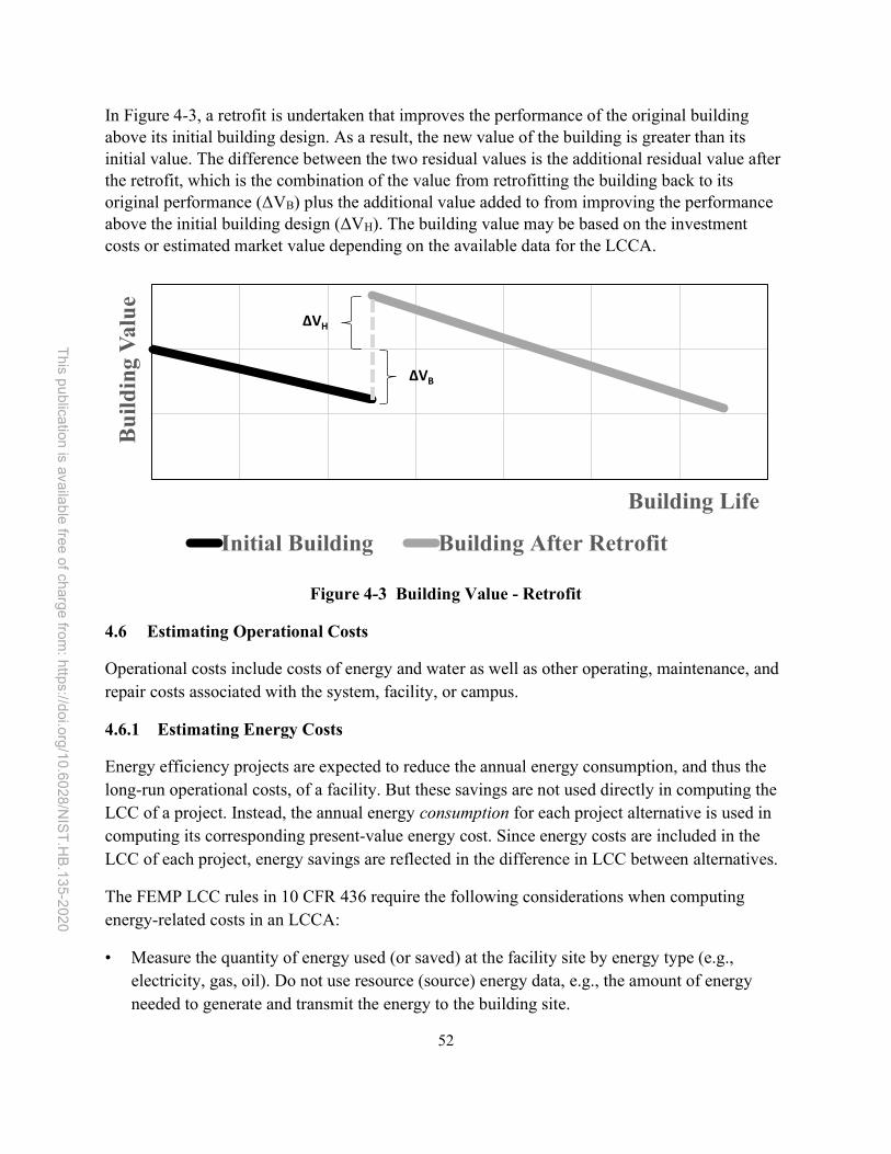
52

This p

ublica

tion is ava

ilab

le free

of ch

arge

from: h

ttps://doi.o

rg/1

0.6

028

/NIS

T.H

B.13

5-202

0

In Figure 4-3, a retrofit is undertaken that improves the performance of the original building above its initial building design. As a result, the new value of the building is greater than its initial value. The difference between the two residual values is the additional residual value after the retrofit, which is the combination of the value from retrofitting the building back to its original performance (ΔVB) plus the additional value added to from improving the performance above the initial building design (ΔVH). The building value may be based on the investment costs or estimated market value depending on the available data for the LCCA.

Figure 4-3 Building Value - Retrofit

4.6 Estimating Operational Costs

Operational costs include costs of energy and water as well as other operating, maintenance, and repair costs associated with the system, facility, or campus.

4.6.1 Estimating Energy Costs

Energy efficiency projects are expected to reduce the annual energy consumption, and thus the long-run operational costs, of a facility. But these savings are not used directly in computing the LCC of a project. Instead, the annual energy consumption for each project alternative is used in computing its corresponding present-value energy cost. Since energy costs are included in the LCC of each project, energy savings are reflected in the difference in LCC between alternatives.

The FEMP LCC rules in 10 CFR 436 require the following considerations when computing energy-related costs in an LCCA:

• Measure the quantity of energy used (or saved) at the facility site by energy type (e.g., electricity, gas, oil). Do not use resource (source) energy data, e.g., the amount of energy needed to generate and transmit the energy to the building site.

Bu

ildin

g V

alu

e

Building Life

Initial Building Building After Retrofit

ΔVH

ΔVB

53

This p

ublica

tion is ava

ilab

le free

of ch

arge

from: h

ttps://doi.o

rg/1

0.6

028

/NIS

T.H

B.13

5-202

0

• Use current, local, energy price schedules for the type of fuel or energy used. Do not use national or regional average prices.

• Use NIST/DOE energy price escalation rates (e.g., those from EERC) unless you have projected escalation rates from the utility supplying the energy.

FEMP does not currently provide specific guidance for estimating future energy prices for federal projects being constructed outside the United States. Other countries currently do not have an EIA equivalent organization that provides public, transparent projections and forecasts of energy prices that could be used as the basis for country or regional escalation rates. The same general approach should be applied in which the analyst should use the best available data.

4.6.1.1 Quantity of Energy Used

Estimating annual amounts of energy required for a given facility system (or for the entire facility) with and without an energy efficiency project is primarily an engineering exercise. These estimates can be based on technical specifications, energy-estimating formulas, or computer simulations.

Energy consumption amounts should be estimated for each type of energy used by the facility or system being evaluated. In the simplest case, where there is a flat-rate energy price, annual energy quantities will be sufficient. However, if different prices are in effect during different usage periods (e.g., summer and winter), estimates of energy usage in each time period will also be needed. And if demand charges are relevant, monthly power demand peaks must also be estimated.

Computer simulation programs such as EnergyPlus (DOE, 2019b) or software tools that use these simulation engines, such as OpenStudio (NREL, 2019a), can be used to estimate energy usage in buildings over an entire year. When selecting a program, it is important to match the capabilities of the program to the type of building and systems to be evaluated. It is also important to consider whether you need annual, monthly, or hourly energy consumption data (and monthly power demand data, most commonly) for computing energy costs. For example, if time-of-use rates are relevant, you must have hourly energy consumption data; monthly estimates will not be sufficient. You should use engineering judgment to verify that estimates of energy usage and corresponding energy savings for project alternatives are reasonable and consistent before proceeding to the economic analysis.

4.6.1.2 Local Energy Prices

Energy prices are needed to convert energy usage to annual energy costs. The FEMP LCC rules require that an LCCA of an energy conservation project be based on actual energy prices effective at the facility site rather than on regional or national average prices. Unit prices as billed by the local utility (or fuel delivery company), including relevant taxes or surcharges,

54

This p

ublica

tion is ava

ilab

le free

of ch

arge

from: h

ttps://doi.o

rg/1

0.6

028

/NIS

T.H

B.13

5-202

0

should be used in computing annual costs for each fuel type used. The appropriate energy prices should be based on the utility's rate schedule effective on the base date of the study, even if the service period (and thus energy usage) does not begin until some later time. The FEMP methodology starts with energy prices as of the base date and converts those prices to their future cost equivalent in each year of the service period using price escalation rates for the specific fuel type, rate type, and region.

The appropriate energy price to be used in computing annual energy costs depends on the nature of the project alternatives to be evaluated. In cases where an energy conservation project changes the amount of a specific energy type used, and unit prices vary with usage amounts (e.g., with a declining block rate), the price of the last unit used (aka, the “marginal” unit) in each billing period is the most appropriate energy price for the analysis. On the other hand, if two systems using different fuel types are being compared, the average unit price is more relevant. In this latter case, there may be no energy savings, just a switch in fuel types.

Other factors that should be considered in estimating annual energy costs (especially about electricity usage) are:

• summer and winter rate differences • time-varying pricing (TVP, including day-ahead, real-time, and time-of-use prices) • block rates • demand charges • Other non-consumption-based charges

The inclusion of these rate factors in an economic analysis may require energy usage data by month instead of by year, and in the case of time-varying pricing, energy usage must be estimated on an hourly (or potentially even more frequent) basis. For most government facilities, peak power demand data, usually monthly, is needed to estimate demand charges. Other local utility programs (e.g., demand response initiatives such as interruptible rates or “capacity” programs) should also be considered. You do not need to include fixed monthly energy charges (e.g., the "customer charge") in the energy cost analysis unless you are comparing systems using different fuel types.7

Section 9.3 provides examples of how to compute annual energy costs when applicable rates depart from flat unit energy pricing.

If annual energy consumption for a project is not expected to be constant over the entire service period, it will be necessary to compute annual energy costs separately for each year and discount these annual costs to present value individually as single amounts. BLCC facilitates this process

7 BLCC 5.3 includes annual kWh usage and kW demand data for a project alternative and does not provide more complex monthly or hourly rate calculations. A user can pre-process the annual cost values before inclusion into BLCC.

55

This p

ublica

tion is ava

ilab

le free

of ch

arge

from: h

ttps://doi.o

rg/1

0.6

028

/NIS

T.H

B.13

5-202

0

by allowing the annual energy usage amounts to be scaled up or down from a base amount. An example of non-constant annual energy usage calculations is shown in Chapter 9.

4.6.1.3 DOE Energy Price Escalation Rates

FEMP rules require that NIST/DOE energy price escalation rates be used in LCC analyses of federal energy conservation and renewable resource projects. These rates are incorporated in the FEMP UPV* factors for energy costs found in the Annual Supplement to Handbook 135. You do not need to compute future energy prices when computing an LCC for a project alternative. This section shows how to compute future energy prices if they are needed for cash flow projections or for computing payback measures that include energy price escalation.

Following the FEMP convention for calculating life-cycle costs in constant-dollar terms, you need to account for real energy price escalation rates when computing future energy costs. The energy price escalation rates provided by NIST/DOE (as published each year in the Annual Supplement to Handbook 135 and as used in BLCC) are real rates. To estimate future energy costs in constant dollars, use the appropriate energy price indices in Table Ca-1 through Table Ca-5 of the Annual Supplement to Handbook 135 to adjust energy prices as of the base date.

Example: If the price for residential electricity in Census Region 1 as of the base date (2019) is $0.082/kWh, and the price index for electricity rates for the year 2020 is 1.01, then the constant-dollar estimate of the electricity price in the year 2020 is

$𝟎. 𝟎𝟖𝟐𝟎/𝒌𝑾𝒉 ∙ 𝟏. 𝟎𝟏 = $𝟎. 𝟎𝟖𝟐𝟖/𝒌𝑾𝒉.

When using the Ca tables in the Annual Supplement to Handbook 135, be sure to find the index that is appropriate to the DOE region, fuel type, rate type, and number of years in your analysis. Note that these price indices represent only real changes in prices from the base date (i.e., net of general inflation) since they are calculated in constant dollars. The price indices should be normalized so that the index for the energy price index at the base date is 1.0.

If you use real energy price escalation rates in a current-dollar analysis, you need to include the estimated annual rate of inflation with those rates. Tables S-1 through S-5 in the Annual Supplement to Handbook 135 provide price indices for inflation rates of 3 %, 4 %, 5 %, and 6 %; you can use those price indices to estimate future energy costs in current dollars in the same way shown above for the constant dollar indices.

4.6.2 Estimating Water Costs

Water costs should be handled much like energy costs. There are usually two types of water costs: water usage and water disposal/treatment. Each of these types may have its own unit costs and price escalation rates. Water prices may also be subject to block rates. When block rates are used, it is generally the price of the last block of usage (i.e., the “marginal” block) in each pricing

56

This p

ublica

tion is ava

ilab

le free

of ch

arge

from: h

ttps://doi.o

rg/1

0.6

028

/NIS

T.H

B.13

5-202

0

period that is most relevant for a water conservation project. The amount of water used or conserved should be measured at the facility site. The water price schedule should also be the schedule in effect at the site. Do not use regional or national average water prices. There are no NIST/DOE water price escalation rates. FEMP (2019f) provides guidance on water and wastewater price escalations as part of its broader guidance on price escalation rates.8 Three estimation methods are acceptable: direct forecast from the serving utility, historical rate data (with cap), or historical consumer price index data. The preferred approach is to use published information from the service utility on price projections. The second option is to use eight years of historical rate data and estimate an average annual escalation rate with a maximum rate of 4.1 % for water supply and 3.3 % for wastewater. The third option assumes escalation occurs at the rate of general inflation. In such a constant dollar analysis you can use the standard UPV factors published in Table A-2 of the Annual Supplement to Handbook 135. (This is the same table of factors used for non-fuel OM&R costs.) For more guidance details, see FEMP (2019f).

FEMP does not currently provide specific guidance for estimating future water prices for federal projects being constructed outside the United States. Other countries currently do not have an EIA equivalent organization that provides public, transparent projections and forecasts of water prices that could be used as the basis for country or regional escalation rates. The same general approach should be applied in which the analyst should use the best available data.

Water costs, like energy costs, are assumed to begin with the service date and continue through the service period until the end of the study period. Water use in the construction phase of a project is not explicitly included in the LCCA of a water conservation project but should be included in the initial investment cost.

4.6.3 Estimating Other Operating, Maintenance, and Repair Costs

Operating, maintenance, and repair (OM&R) costs are often more difficult to estimate than other building expenditures. Since operating schedules and standards of maintenance vary from facility to facility, there is great variation in these costs, even for facilities of the same type and age. It is therefore especially important to use engineering judgment when estimating these costs.

OM&R costs generally begin with the service date and continue through the service period. Some OM&R costs are annually recurring costs that are constant from year to year or change at some estimated annual rate. The present value of annually recurring costs over the entire service period can be estimated using appropriate UPV or UPV* factors (See Section 3.2.2.). Others are single costs, occurring only once or at non-annual intervals throughout the service period. These must be discounted individually to present value (See Section 3.2.1.).

8 Guidance is based on FEMP (2017b)

57

This p

ublica

tion is ava

ilab

le free

of ch

arge

from: h

ttps://doi.o

rg/1

0.6

028

/NIS

T.H

B.13

5-202

0

4.6.3.1 Estimating OM&R Costs from Cost-Estimating Resources

Ongoing efforts to standardize OM&R costs have produced several helpful manuals and databases, examples of which are listed in Table 4-1. Keep in mind that if OM&R costs are essentially the same for each of the project alternatives being considered, they do not have to be included in the LCCA.

Some of the data estimation guides listed in Table 4-1 (Building Owners and Managers Association (BOMA), RSMEANS) derive cost data from statistical cost-estimating relationships of historical data. They then report, for example, average owning and operational costs per square foot, by age of building, geographic location, number of stories, and number of square feet in a building. The Construction Engineering Research Laboratory (CERL) M&R Database derives data from time-motion studies, which estimate the time required to perform certain tasks. It covers four major building systems (architectural, electrical, plumbing, and HVAC) and provides indices for estimating the cost of keeping selected building components in good service condition. At the lowest level of data aggregation, the CERL database provides data for about 3000 typical tasks needed to maintain and repair building components.

4.6.3.2 Estimating OM&R Costs from Direct Quotes

A more direct method of estimating non-fuel OM&R costs is to obtain quotes from contractors and vendors. For cleaning services, for example, you can get quotes from contractors based on prevalent practices in similar buildings. Maintenance and repair estimates for equipment can be based on manufacturers' recommended service and parts replacement schedules. You can establish these costs for the initial year by obtaining direct quotes from suppliers. For a constant-dollar analysis, the annual amount will be the same for the future years of the study period, unless, as is sometimes the case, OM&R costs are expected to rise as the system ages. In this latter case, the real (differential) escalation rate for that cost must also be included in the analysis.

4.7 Estimating Other Benefits and Costs

Other benefits and costs may include a range of categories, including direct financial effects (e.g., rebates, taxes, and financing costs), indirect financial effects (e.g., increased available space, higher rents), and “difficult-to-quantify” (non-monetary) effects (e.g., greater productivity, improved occupant health, lower environmental impacts). These benefits and costs are particularly important for project scopes at the building, facility, and campus levels because of the multitude of interactions that may occur across systems. These costs have been explicitly introduced into the LCC formulas as “other costs,” (labeled as “X” as suggested by M. Zhivov (2020)).

4.7.1 Direct Financial Benefits and Costs

Direct benefits and costs that could influence a project include financial incentive programs, taxes, and financing costs. Utility companies frequently offer energy incentive programs, such as

58

This p

ublica

tion is ava

ilab

le free

of ch

arge

from: h

ttps://doi.o

rg/1

0.6

028

/NIS

T.H

B.13

5-202

0

demand side management incentives and rebates to promote investment in more energy-efficient facilities, which are generally available to federal agencies. If a rebate is granted after the base date of the study, you need to discount it to present value - just like any other cost or benefit - before subtracting it from initial investment costs. Since this handbook focuses on projects in federal buildings, taxes need not be taken into consideration. Likewise, the cost of financing projects can be disregarded in an LCCA of this type unless the financing is specifically tied to the project. For example, the LCCA of a project using appropriated funds does not account for the cost to the federal government from borrowing money to provide those funds. If financing is provided via an energy savings performance contract (ESPC) or utility energy service contract (UESC), specific requirements related to evaluating cost-effectiveness apply. See Chapter 10 for more information on alternative financing options for federal projects. In private-sector analyses, these factors should be included if they are expected to make a significant difference in the outcome of the analysis.

4.7.2 Indirect Financial Benefits and Costs

LCCA is most appropriately used to evaluate the relative costs of design alternatives that satisfy a set of performance requirements. It is not generally appropriate for evaluating the cost-effectiveness of alternative revenue-producing projects, such as buildings constructed to produce rental income. For example, you would not typically use an LCCA to determine whether to build a 20-unit apartment building or a 40-unit building because the occupancy requirement is different (e.g., 20 households versus 40 households). However, if there are differences in revenue between one design alternative and another, they can be included in the LCCA by adding them to (when negative) or subtracting them from (when positive) annual operation-related costs. For example, retrofitting a building may lead to additional available office space that provides a financial value as reduced rental costs or increased rents.

The term “indirect” financial costs, in this context, refers to costs not directly related to constructing and operating the building itself, which has thus far been the focal point of this handbook. Ultimately, a building’s purpose is to provide an effective indoor environment for its occupants. In the case of residential space (e.g., houses and apartments), the goal is to provide a comfortable, safe living environment to the occupants. In the case of workspace (e.g., office buildings), the goal is to provide the most conducive environment for productivity. In either case, there are potential benefits to building occupants from a higher performing design, whether the performance is related to resource efficiency, sustainability, resilience, or safety and security.

Whether it’s selecting a higher performing building design for new construction, choosing to lease a high-performance property, or renovating a building above and beyond the prior design with a deep energy retrofit (DER) (i.e., greater than 30 % reduction in energy consumption), federal agencies (e.g., GSA) will need to justify the higher initial costs or rents. Studies have shown that higher performing (specifically energy efficient- and green-rated) buildings lead to higher values for those spaces, whether that is through premiums on rents or resale values. These premiums may be driven by a combination of two factors: financial and ideological (Zhang, Wu, & Liu, 2018). Financially, buildings with high performance certifications are expected to reduce

59

This p

ublica

tion is ava

ilab

le free

of ch

arge

from: h

ttps://doi.o

rg/1

0.6

028

/NIS

T.H

B.13

5-202

0

operational costs while improving occupant health, comfort, and productivity. Ideologically, some individuals and organizations will have non-economic preferences for the benefits resulting to society from high performance buildings (resource conservation, environmental impact reduction, and human health prioritization). It is difficult to isolate the fraction of the premium associated with these two factors with the literature to date.

A summary of the literature, which has focused on green and energy efficient buildings, will be included below to provide some guidance on the potential indirect benefits but should not be used as precise data to be implemented in a LCCA for federal buildings. Instead the information can provide values for consideration when considering projects that are not deemed cost-effective while excluding these benefits. If values for these indirect benefits are included, a sensitivity analysis should be completed to ensure the assumptions are not driving the final decision.

4.7.2.1 Rental and Sale Premiums

Higher performing office buildings have been shown to earn premiums, both rents and sale prices, in the market. These premiums have financial implications for the government for new and retrofit construction projects and should be considered when evaluating the cost-effectiveness of federally owned or leased buildings. Estimating the additional value of either new construction or retrofit project on a federally owned facility should be included in a LCCA by including it in the residual value of the building consistent with the residual value method implemented for other capital investments as discussed in Section 4.5.3.

Five studies (Eichholtz, Kok, & Quigley, 2010, 2013; Fuerst & McAllister, 2011a, 2011b; Wiley, Benefield, & Johnson, 2010), summarized in Zhang et al. (2018), have analyzed rental and sales data for EnergyStar and U.S. Green Building Council (USGBC) Leadership in Energy and Environmental Design (LEED) certified office buildings in the United States. The rental premiums have a wide range depending on the study, with EnergyStar-certified office buildings get a 3.0 % to 10.5 % rental premium and LEED-certified buildings get a 4.1 % to 18.9 % premium. Similar results are found in the building sale data for EnergyStar (5.1 % to 31.0 %) and LEED (11.7 % to 28.4 %) certified buildings. Additionally, buildings receiving the highest LEED rating (platinum) realized the greatest rental and sale premiums. These publications as well as others are also summarized Jungclaus et al. (2017), Lohse and Zhivov (2019), and RMI (2015b), which are focused on energy efficiency studies that have implications for energy efficiency retrofits that achieve at least 30% energy savings in a building, often referred to as DER. The rental premium range is stated at 2.1 % to 17.0 % while sale premiums are 11.1 % to 26.0 %. Bleyl et al. (2019) estimates rental and sales premiums from DER projects to be 1.0 % to 5.3 % and 2.5 % to 6.5 %, respectively. Bond and Devine (2016) finds that green multifamily residential buildings realize an 8.9 % rental premium while other studies have looked at single-family residential buildings (Aroul and Hansz (2012); Kok and Kahn (2012)), showing the results above are not exclusive to commercial space.

60

This p

ublica

tion is ava

ilab

le free

of ch

arge

from: h

ttps://doi.o

rg/1

0.6

028

/NIS

T.H

B.13

5-202

0

DOE’s Building Technology Office (BTO) (DOE BTO, 2017) analyzed 131 commercial office properties owned by a single real estate company to determine if there are statistical differences in market value, net operating income, occupancy, rent, operating expenses, and rent concessions between green and non-green properties. Even with a minimal dataset, the study found statistically significant (>95%) premiums for market value (8.4 %) and net operating income (28.8 %) and lower operating expenses (-17.6 %). Additionally, occupancy rates were marginally statistically significant (>90 %) with 6.2 % higher rate. Rent and rental concessions were not statistically significant, but the magnitude showed higher rents (4.3 %) and lower rental concessions (-6.9 %).

Dodge Data & Analytics (2018) analyzes data collected by a worldwide survey in 2018 related to the green building market. Customer demand and environmental regulations are the primary drivers of green construction in U.S. with a focus on occupant health and well-being while concerns remain focused on first costs and overall affordability. Appropriately estimating the added value of green construction could alleviate those economic concerns. Of all respondents, 74 % stated that new green buildings have higher initial costs with 79 % stating the simple payback for green buildings is less than 10 years. The respondents also viewed new green buildings to have a higher asset value, with 83 % (30 %) of owners and 63 % (27 %) of architects and contractors expecting at least a 3 % (10 %) increase, respectively. Of all respondents, 82 % stated that green retrofits have a simple payback less than 10 years and higher asset values with 41 % (14 %) of owners and 62 % (34 %) of architects and contractors expecting at least a 5 % (10 %) increase, respectively. Owners appear to view new green buildings better than retrofits while architects and contractors view retrofits as the better investment. U.S. respondents reported an expected payback for green investments of seven years.

Estimating the rental or sale premium resulting from improving the performance of a building will be dependent on the market in which the building is located. If local real estate market data is available, it should be used as the basis for any premium estimate. If local data is not available, a reasonable conservative proxy would be the lower end estimates above. However, a sensitivity analysis should be completed to ensure the results are not overly sensitive to the premium assumption.

Occupancy rates are not as much of a concern from a federal agency perspective because either the federal government owns the building and uses 100 % of the space or it is leasing the building and is not concerned about whether the 3rd-party owner is maximizing occupancy of the other units in the building.

4.7.2.2 Productivity and Space Utilization Gains

In the case of a leased property, a government agency may need to justify the higher rental rates. As with customer owned buildings this can sometimes be accomplished using operational savings (e.g., energy and water cost savings, lower O&M costs). However, it may be appropriate to include indirect benefits in the LCCA if there is a clear gain being excluded from the analysis. Labor costs are typically the largest cost category for an organization, often by a wide margin.

61

This p

ublica

tion is ava

ilab

le free

of ch

arge

from: h

ttps://doi.o

rg/1

0.6

028

/NIS

T.H

B.13

5-202

0

Worker productivity gains have been shown to potentially overwhelm any additional costs associated with building indoor environment improvements.

As summarized in Zhang et al. (2018), green-rated buildings have been shown to improve productivity by 6 % to 25 % as well as reducing absenteeism by 15 % to 25 % (Bragera & deDear, 1998; Kats, Alevantis, Berman, Mills, & Perlman, 2003; Paul & Taylor, 2008; Ries, Bilec, Gokhan, & Needy, 2006; Romm & Browning, 1998). These productivity gains are typically related to improvements in better quality lighting that improves visual acuity and better thermal comfort, including personalized control of the lighting and ambient environment. Similarly, Loftness, Hartkopf, and Gurtekin (2003) summarizes the literature on worker productivity gains from improved indoor environments: 0.4 % to 18 % productivity gains from access to the natural environment (daylight and operable windows), 0.7 % to 23.0 % gains for better lighting, 0.48 % to 11.0 % gains from better ventilation, and 0.2% to 3.0 % gains from individual temperature control. Bleyl et al. (2019) estimates work productivity increases from DER projects to be 0.57 % to 1.14 %.

The use of a well-defendable, conservative estimate for productivity gains and reduced absenteeism could be combined with labor rates to estimate the indirect benefits to the organization. As with other indirect benefits and costs, the productivity gains will vary significantly by project. A sensitivity analysis should be completed to ensure the results are not overly sensitive to the productivity assumption.

Space utilization could have significant impacts on a building’s value and occupant health, comfort, and productivity. Redesigning the floor layout could help to provide occupants with better indoor environmental conditions that improve productivity. Additionally, a building retrofit could lead to more effective use of the available space in the building, either providing the same number of occupants with better office and shared spaces (and therefore productivity) or increase the number of occupants in the same building footprint (while maintaining productivity and occupant well-being). In the case of the prior, the impact may be included in the productivity improvement estimate while the latter can be estimated using the value of the increased space based on the savings to the organization from not renting that space elsewhere.

Occupant satisfaction can be used as a measure of indirect benefits from a higher performing building. However, quantifying these benefits is difficult. There is likely to be a strong relationship between occupant satisfaction and productivity. Therefore, the inclusion of productivity in the analysis will likely capture some of the benefits of improved occupant satisfaction. For more on occupant satisfaction, see Section 4.7.3.

4.7.2.3 Risk Mitigation

Thus far, the focus has been on the benefits and costs of typical operating conditions. However, resilience could be an important objective of a project. Risk mitigation from uncommon and/or extreme events (e.g., energy security, extreme weather events, geological conditions) could provide additional benefits to an agency not captured in a traditional LCCA that would treat resiliency as a minimum requirement and, therefore, a restricting condition on feasible

62

This p

ublica

tion is ava

ilab

le free

of ch

arge

from: h

ttps://doi.o

rg/1

0.6

028

/NIS

T.H

B.13

5-202

0

alternatives. However, one of the feasible alternatives may provide higher resilience performance than the minimum requirement, which provides some expected benefits (based on the probability of events and the value of reducing the risk) that should be included in the analysis.

Anderson et al. (2016) defined two general approaches to estimate the cost of a grid interruption: macroscopic and microscopic. Macroscopic value estimation uses historical national or utility level outage cost estimates, requiring less data but often does not capture location-specific costs. Microscopic value estimation uses a survey of the location-specific outage costs, which may be more accurate but is a time-consuming process.

NIST has published the Community Resilience Economic Decision Guide for Buildings and Infrastructure Systems that can assist a decisionmaker in considering benefits and costs of risk mitigation (Gilbert, Butry, Helgeson, & Chapman, 2015). The guide categorizes resilience benefits into reductions in disaster costs and losses, non-disaster related benefits, and externalities. Disaster related cost examples include loss of life, injuries, and damages to infrastructure. By improving resilience with higher initial investments, it is possible to lower the expected future losses from a potential disaster. Indirect benefits might include reductions in mission interruption losses due to non-hazard-related power or water outages. For example, burying powerlines to prevent failure due to ice or wind decreases the need and cost for right of way vegetation trimming. Some indirect effects may be negative. For instance, buried power lines are more susceptible to flooding, cannot be visually inspected, and can be more expensive to repair if damage does occur. The guide and the resulting ASTM standard (ASTM E3130, 2018) can assist in defining such probability distributions and risk preferences.

DoD has particular interest in risks associated with their coastal military facilities, and published a report on regional sea level scenarios to evaluate coastal risk management (Hall et al., 2016). This report developed a scenario database that provided regionalized sea level and extreme water level scenarios for three time horizons (2035, 2065, and 2100) that cover 1774 DoD military facilities worldwide facing coastal or tidal risks. The report includes case studies for the purpose of highlighting potential applications of the developed scenarios in the context of specific circumstances.

Projects that include safety and security aspects, which also involve evaluating rare, high impact events, can be included in the analysis in a similar manner to resilience. In many cases the benefits of resilience and other risk mitigation related decisions are unknown and/or difficult to quantify, let alone monetize into a present value estimate. In such cases, non-monetary values should be provided in the analysis.

4.7.3 Non-Monetary Benefits and Costs

“Difficult-to-quantify,” or non-monetary, benefits and costs are project-related effects for which it is difficult to objectively assign a dollar value. These benefits and costs are most likely indirect or external. In some cases, indirect benefits and costs may be included under non-monetary benefits and costs because there are not reliable economic values for use in the analysis. Instead these benefits and costs should be included at either non-monetary quantitative metrics or a

63

This p

ublica

tion is ava

ilab

le free

of ch

arge

from: h

ttps://doi.o

rg/1

0.6

028

/NIS

T.H

B.13

5-202

0

qualitative metric or description. Examples of indirect non-monetary effects may be improved collaboration due to improved space optimization from the building retrofit or higher occupant satisfaction from a quieter HVAC system. External non-monetary effects are even more abstract, such as reduced environmental impacts from reduced resource consumption and associated emissions. These items, by their nature, are external to the LCCA, and thus do not directly affect the calculation of a project's cost-effectiveness. Nevertheless, you should consider significant non-monetary effects in your final investment decision, and they should be included in the project documentation.

For a project having an LCC greater than its base case (which would thus be rejected on a dollar cost basis), but having significant non-monetary benefits, you can subjectively judge whether the non-monetary benefits outweigh the LCC penalty. If the decision-maker judges that the non-monetary benefits of a project are greater than its LCC penalty, the project can be accepted as "cost-effective."

4.7.3.1 Monetizing Non-Monetary Benefits and Costs

Non-monetary benefits and costs may not have an objective monetary value. However, there are economic approaches that can be used to provide order-of-magnitude dollar value of a subjective benefit or cost in some instances. Gilbert et al. (2015) identified two non-market valuation approaches, contingent value surveys (stated preference approach) and the hedonic valuation method (indirect or revealed preference approach) that estimate “how much people are willing to pay for the utility they obtain from a particular non-market good.” Murakami, Itsubo, Kuriyama, Yoshida, and Tokimatsu (2018) is an example from the literature that developed weighting factors for estimating willingness to pay for reducing environmental damages. These approaches are applicable for any non-market good, such as occupant satisfaction and happiness. External non-monetary benefits and costs, such as pollution, sometimes have formal markets that can be used to estimate their value either regionally or nationally (SO2 and NOX). These types of estimates may require significant time and effort to identify and should only be undertaken if it is deemed to have a significate impact on the decision.

4.7.3.2 Non-Monetary Metrics

In the case of benefits and costs that cannot be valued in economic terms, a non-monetary metric should be identified and used whenever possible. For example, if no productivity value can be determined, the analysis should include metrics related to productivity, such as occupant satisfaction, IAQ and thermal comfort measurements, and reduced absenteeism (sick days). This can be referred to as a mid-point estimate that measures the effect but does not associate an economic impact. For example, GSA (2011) found that in 22 sustainably designed buildings occupant satisfaction increased 27%, on average, relative to the national average with none rating below the national average. Examples from resilience-related projects include time to recovery, hours of mission-critical service outages, and lives lost. While these measures can sometimes be evaluated through a statistical value, the required data may not be available or interested parties may prefer non-economic measures (e.g., value-of-a-statistical life can be

64

This p

ublica

tion is ava

ilab

le free

of ch

arge

from: h

ttps://doi.o

rg/1

0.6

028

/NIS

T.H

B.13

5-202

0

considered controversial). These types of values can demonstrate the non-monetized benefits and costs in a manner that can be understood and considered by a decisionmaker.

External benefits and costs should be reported in a well-accepted metric. A common science-based methodology to account for non-monetary environmental and human health impacts is life cycle assessment (LCA). LCA is a comprehensive method that can be used to evaluate environmental impacts associated with the full life cycle of a product from raw material extraction to materials processing and manufacturing, distribution, use, and disposal or recycling. If the external impacts are of importance to the decision maker, an LCA could be completed to determine the incremental change in the impact categories of interest.

The most widely adopted set of impact categories is EPA’s TRACI 2.1, which includes models for a variety of impact categories, including ozone depletion potential, global warming potential (GWP), acidification potential, eutrophication potential, smog formation potential, human health impacts, ecotoxicity, and fossil fuel depletion (Environmental Protection Agency, 2018). Each impact category has a common unit of measure defined to allow for multiple pollutants to be combined into a single equivalent value with respect to the environmental impact considered. For example, GWP is reported in CO2 equivalence (CO2-eq) over 100 years. Methane (CH4) is estimated to have a GWP of 28–36 over 100 years.9 The total methane released are multiplied by the appropriate factor to get the total CO2-eq for those emissions. Each GWP-related pollutant goes through the same process and then are summed to calculate the total GWP. These non-monetary metrics are considered “mid-point” estimates because they quantify the environmental impact but do not provide an economic value to the resulting damages.

The different units of measure make it difficult to compare results across impact categories. One approach to address this issue is to develop a pair-wise comparison using the Analytical Hierarchy Process (AHP) defined in ASTM Standard E1765 that incorporates the priorities of the decisionmaker to make a qualitative judgement on different metrics (ASTM, 2016). DoD also provides guidance for quantifying qualitative metrics in its Benefit-Cost Analysis (BCA) analysis (DoD, 2014). Researchers are also working on quantifying these resulting damages (Murakami et al., 2018; Pizzol, Weidema, Brand, & Osset, 2015). An example of converting LCA results to economic values and incorporating those values into a LCCA will be provided in Section 12.1.3.

For non-monetary benefits and costs that do not have a clear metric for reporting, provide a description of the benefit or cost that clearly explains what it is and why it is important for the decision-making process.

9 Source: https://www.epa.gov/ghgemissions/understanding-global-warming-potentials

65

This p

ublica

tion is ava

ilab

le free

of ch

arge

from: h

ttps://doi.o

rg/1

0.6

028

/NIS

T.H

B.13

5-202

0

66

This p

ublica

tion is ava

ilab

le free

of ch

arge

from: h

ttps://doi.o

rg/1

0.6

028

/NIS

T.H

B.13

5-202

0

5 Calculating Life Cycle Costs

In this handbook we define life-cycle cost analysis (LCCA) to include both the LCC method and certain supplementary measures: Net savings (NS), savings-to-investment ratio (SIR), and adjusted internal rate of return (AIRR). LCCA is the standard method required by FEMP for evaluating energy efficiency, water conservation, and renewable energy investments in federal buildings. The FEMP criteria for performing LCCA, as published in 10 CFR 436, are summarized in Table 5-1. The examples in Chapter 5 through Chapter 7 integrate LCCA and the FEMP LCCA criteria.

The basic LCC method is the most straightforward method of accounting for present and future costs of a project over its life cycle. When using the LCC method for evaluating facilities or systems, we typically look at two or more project alternatives for the same purpose (e.g., different R-values of insulation in an exterior wall or different HVAC systems to serve the same load), only one of which will be selected for implementation. To determine the relative cost-effectiveness of these mutually exclusive alternatives, we need to compute the LCC for each alternative and the base case, compare them, and choose the alternative with the lowest LCC. Only when compared to the LCC of a base case or another alternative intended for the same purpose does the LCC provide useful information. The LCCs are comparable only if computed with the same economic assumptions and with the same study period, base date, and service date. In addition, it is essential that only alternatives that satisfy minimum performance requirements be considered for LCCA.

This chapter first describes the LCC method and then illustrates how to compute the life-cycle costs for a base case and an alternative. Chapter 6 explains how to calculate supplementary measures - net savings (NS), savings-to-investment ratio (SIR), adjusted internal rate of return (AIRR), and discounted and simple payback. Chapter 7 demonstrates how these methods can be applied to typical cost-effectiveness decisions related to energy efficiency, water conservation, and renewable energy projects in federal facilities.

5.1 Life-Cycle Cost (LCC) Method

LCCA allows you to organize and compute the costs of acquiring, owning, operating, maintaining, and ultimately disposing of a facility, system, or piece of equipment. Once you have cost estimates, by year, for two or more competing alternatives, a discount rate, and a defined study period (i.e., starting point and number of years), you are ready to calculate the LCC for each alternative.10 To calculate the LCC, first compute the present value of each cost to be incurred during the study period, using the DOE discount rate. Then sum these present values for each alternative to find its LCC. If other performance features are similar among the alternatives, the alternative with the lowest LCC is the preferred alternative; that is, it is the most cost-effective alternative for the application studied.

10 All through this handbook we use the word "alternative" to include the base case when discussing the LCC method.

67

This p

ublica

tion is ava

ilab

le free

of ch

arge

from: h

ttps://doi.o

rg/1

0.6

028

/NIS

T.H

B.13

5-202

0

The calculations can be performed either manually or with a computer program. BLCC, which can greatly facilitate FEMP LCC analyses for energy efficiency, water conservation, and renewable energy projects, integrates the FEMP criteria and is largely self-documenting. More information about BLCC is presented in Chapter 16. Simple analyses can be done manually in a spreadsheet program (e.g, Excel).

Table 5-1 Summary of Criteria for FEMP LCCA

Methodology Evaluation Method Life-cycle cost analysis Discounting Approach Present value (PV) at the base date Cost Measurement Basis Constant dollars as of the base date Cash-Flow Convention End-of-year cash flows or when incurred

Evaluation Criteria

Lowest life-cycle cost Highest net savings SIR > 1 for ranking AIRR > FEMP discount rate for ranking

Uncertainty Assessment Sensitivity analysis Data and Parameters Base Date Date of study / beginning of study period

Service Date Beginning of service period when building is occupied or system taken into service

Study Period Planning / construction period (if any) added to maximum 40-year service period

Discount Rate Real rate, determined annually by DOE

Energy Prices Local energy prices at the building site used to calculate annual energy costs for each energy type

Cost Escalation

• Energy Prices

• Non-Energy Prices

• DOE-projected differential energy price changes (FEMP UPV* discount factors by energy type)

• 0% differential price change (unless justified by reliable projections)

Documentation

Basic Requirement Written record for every economic analysis

Format BLCC computer printouts; worksheets, additional records

5.1.1 General Formula for LCC

The following is the general formula for the LCC present value model:

𝐿𝐶𝐶 =𝐶

(1 + 𝑑)(5 − 1)

68

This p

ublica

tion is ava

ilab

le free

of ch

arge

from: h

ttps://doi.o

rg/1

0.6

028

/NIS

T.H

B.13

5-202

0

Where: LCC = Total LCC in present-value dollars of a given alternative Ct = Sum of all relevant costs, including initial and future costs, less any positive

cash flows, occurring in year t, N = Number of years in the study period d = Discount rate used to adjust cash flows to present value

5.1.2 LCC Formula for Building-Related Projects

The general LCC formula shown in Equation 5-1 requires that all costs be identified by year and by amount. This general formula is straightforward from a theoretical standpoint but can require extensive calculations. This is especially true when the study period is more than a few years long and there are annually recurring amounts for which future costs must first be calculated to include changes in real (i.e., constant dollar) prices. A simplified LCC formula for computing the LCC of projects in buildings can be stated as follows:

𝐿𝐶𝐶 = I + Repl − Res + E + W + OMR + X (5 − 2) where: LCC = Total LCC in present-value dollars of a given alternative I = Present-value investment costs Repl = Present-value capital replacement costs Res = Present-value residual value (resale value, scrap value, salvage value) less

disposal costs E = Present-value energy costs W = Present-value water costs OMR = Present-value non-fuel operating, maintenance, and repair costs X = Present-value other costs (benefits treated as negative costs)

Note that this formula includes an “other costs” category, which has been added to explicitly introduce other monetary benefits and costs that have historically been excluded (e.g., productivity, human health) as determined appropriate by the analyst or specified by agency guidance. This remains consistent with ASTM Standard E917.

This formula takes advantage of UPV (uniform present value) factors to compute the present value of annually recurring costs, whether constant or changing. By using appropriate UPV factors, the LCC can be calculated without first computing the future annual amount (including price escalation) of each annually recurring cost over the entire study period, summing all those costs by year and discounting them to present value. Instead, only the annual amount in base year dollars (i.e., a one-time amount) and the corresponding UPV factor need to be identified.

The following two examples apply the LCC method, combined with the FEMP criteria, to determine whether an investment in energy-saving features for a new HVAC system is economically worthwhile. Example 5-1 assumes that all initial investment costs occur in a lump sum at the base date, that there is only one energy type, and that the two candidate systems have equal useful lives. In Example 5-2, we will relax these assumptions and illustrate an LCC calculation where some of the initial investment costs are phased in during a

69

This p

ublica

tion is ava

ilab

le free

of ch

arge

from: h

ttps://doi.o

rg/1

0.6

028

/NIS

T.H

B.13

5-202

0

planning/construction (P/C) period, where two fuel types are used, and where the two candidate systems have unequal useful lives.

In both these examples, it is assumed that an existing HVAC system in a federally owned facility must be replaced. However, the application of LCCA would be identical for HVAC system selection in a new federal facility. Note that other benefits and costs are assumed to be zero for these examples.

5.2 Example 5-1: Selection of HVAC System for Office Building - Simple Example

We look at a conventional HVAC system as our base case (BC) and compare it with an alternative (A) that includes several energy-saving features. The system with the lower LCC will be accepted as the cost-effective system. The HVAC system is to be installed in a federal office building in Washington, DC. All initial investment costs are assumed to be incurred at the beginning of the study period. The parameters and assumptions common to both the base case and the alternative are as follows:

Location: Washington, DC, Census Region 3 Discount Rate: 2019 FEMP discount rate: 3% real for constant-dollar analysis Energy Prices: Fuel Type: Electricity at $0.12/kWh, local rate as of base date

Rate Type: Commercial Discount Factor: FEMP UPV* factor based on a 3 % (real) discount rate Useful Lives of Systems: 20 years Study Period: 20 years Base Date: January 2019

5.2.1 Base Case – Conventional Design

The base case (BC) is a constant-volume HVAC system with a reciprocal chiller, without economizer cycle. The relevant cash flows as of today, the base date, are:

• $103 000 – initial investment costs assumed to occur in a lump sum • $12 000 – replacement cost for a fan at the end of year 12 • $3500 – residual value at the end of the 20-year study period • $30 000 – annual electricity costs (250 000 kWh at $0.12/kWh) • $7000 – annual OM&R costs

The cash-flow diagram in Figure 5-1 below shows these cost items and their timing for the base case. Initial investment costs are assumed to occur on January 1, 2019. The two other one-time amounts - the fan replacement and the residual value - are assumed to occur at the end of the respective years. Since this is a constant-dollar analysis and no real price escalation (that is, price escalation different from general inflation) is expected for either the fan replacement or the residual value, the 2019-dollar amounts can be used as estimates of the future costs of these items in years 2031 and 2039. Likewise, OM&R costs are expected to remain the same in constant-dollar terms so that equal annual amounts in base-date (January 2019) dollars can be used throughout the study period. As for the electricity cost, the annual amount in base-date

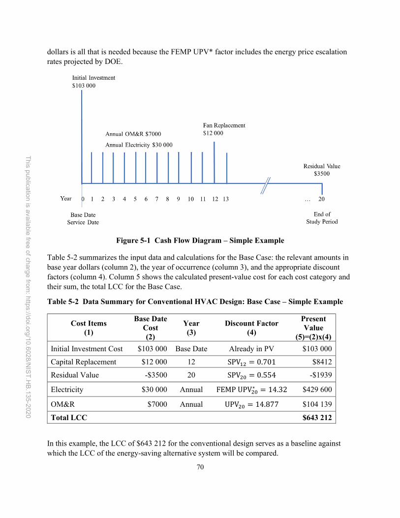
70

This p

ublica

tion is ava

ilab

le free

of ch

arge

from: h

ttps://doi.o

rg/1

0.6

028

/NIS

T.H

B.13

5-202

0

dollars is all that is needed because the FEMP UPV* factor includes the energy price escalation rates projected by DOE.

Figure 5-1 Cash Flow Diagram – Simple Example

Table 5-2 summarizes the input data and calculations for the Base Case: the relevant amounts in base year dollars (column 2), the year of occurrence (column 3), and the appropriate discount factors (column 4). Column 5 shows the calculated present-value cost for each cost category and their sum, the total LCC for the Base Case.

Table 5-2 Data Summary for Conventional HVAC Design: Base Case – Simple Example

Cost Items (1)

Base Date Cost (2)

Year (3)

Discount Factor (4)

Present Value

(5)=(2)x(4)

Initial Investment Cost $103 000 Base Date Already in PV $103 000

Capital Replacement $12 000 12 SPV = 0.701 $8412

Residual Value -$3500 20 SPV = 0.554 -$1939

Electricity $30 000 Annual FEMP UPV∗ = 14.32 $429 600

OM&R $7000 Annual UPV = 14.877 $104 139

Total LCC $643 212

In this example, the LCC of $643 212 for the conventional design serves as a baseline against which the LCC of the energy-saving alternative system will be compared.

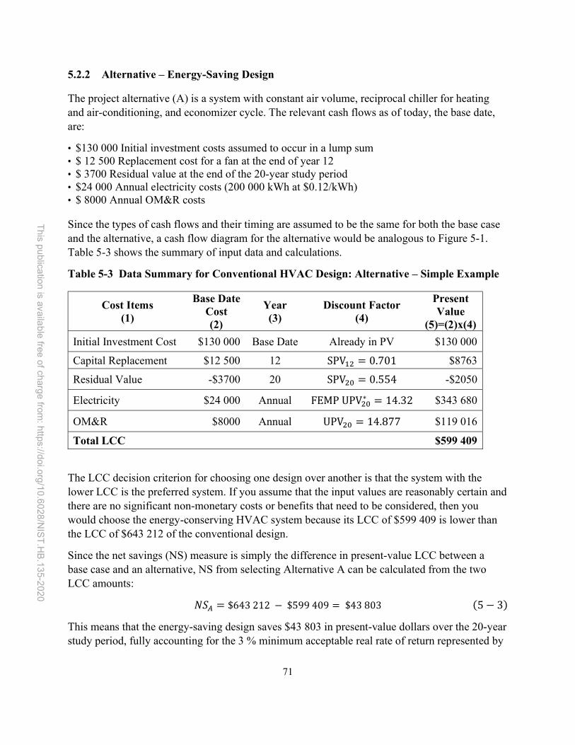
71

This p

ublica

tion is ava

ilab

le free

of ch

arge

from: h

ttps://doi.o

rg/1

0.6

028

/NIS

T.H

B.13

5-202

0

5.2.2 Alternative – Energy-Saving Design

The project alternative (A) is a system with constant air volume, reciprocal chiller for heating and air-conditioning, and economizer cycle. The relevant cash flows as of today, the base date, are:

• $130 000 Initial investment costs assumed to occur in a lump sum • $ 12 500 Replacement cost for a fan at the end of year 12 • $ 3700 Residual value at the end of the 20-year study period • $24 000 Annual electricity costs (200 000 kWh at $0.12/kWh) • $ 8000 Annual OM&R costs

Since the types of cash flows and their timing are assumed to be the same for both the base case and the alternative, a cash flow diagram for the alternative would be analogous to Figure 5-1. Table 5-3 shows the summary of input data and calculations.

Table 5-3 Data Summary for Conventional HVAC Design: Alternative – Simple Example

Cost Items (1)

Base Date Cost (2)

Year (3)

Discount Factor (4)

Present Value

(5)=(2)x(4)

Initial Investment Cost $130 000 Base Date Already in PV $130 000

Capital Replacement $12 500 12 SPV = 0.701 $8763


Electricity $24 000 Annual FEMP UPV∗ = 14.32 $343 680

OM&R $8000 Annual UPV = 14.877 $119 016

Total LCC $599 409

The LCC decision criterion for choosing one design over another is that the system with the lower LCC is the preferred system. If you assume that the input values are reasonably certain and there are no significant non-monetary costs or benefits that need to be considered, then you would choose the energy-conserving HVAC system because its LCC of $599 409 is lower than the LCC of $643 212 of the conventional design.

Since the net savings (NS) measure is simply the difference in present-value LCC between a base case and an alternative, NS from selecting Alternative A can be calculated from the two LCC amounts:

𝑁𝑆 = $643 212 − $599 409 = $43 803 (5 − 3)

This means that the energy-saving design saves $43 803 in present-value dollars over the 20-year study period, fully accounting for the 3 % minimum acceptable real rate of return represented by

72

This p

ublica

tion is ava

ilab

le free

of ch

arge

from: h

ttps://doi.o

rg/1

0.6

028

/NIS

T.H

B.13

5-202

0

the discount rate. If the LCC of an alternative is lower than the LCC of the relevant base case, it must have positive NS.

5.3 Example 5-2: Selection of HVAC System for Office Building - Complex Example

A second example of an LCCA is presented here with more complex analytical requirements. Suppose that the initial cost of the HVAC system in the Base Case of Example 5-l is to be phased in during the two-year P/C period instead of being charged to the project as a lump sum at the beginning of the study period. The study period will be extended to 22 years to include a P/C period of two years and a service period of 20 years. Furthermore, suppose that the useful lives of the two systems are different: 15 years for the base case and 20 years for the alternative. A substantial portion of the base case system will need to be replaced at the end of its useful life of 15 years, at a cost of $60 000, to prolong its useful life to at least 20 years. However, this replacement will increase its residual value to $20 000 at the end of the 20-year study period. Finally, assume that each system uses two different fuel types, electricity and natural gas.

5.3.1 Base Case – Conventional Design – Complex Example

The cash flow diagram in Figure 5-2 reflects the assumptions for the base case. The study period in this example is 22 years because the two-year P/C period is added to the service period of 20 years. The base date is January 1, 2019. Initial investment costs are charged in two installments, at the end of 2019 and end of 2020. Capital replacement costs are charged for the fan unit after 12 years of service (end of 2032) and for plant renovation after 15 years of service (end of 2035). Annually recurring costs, such as energy costs and OM&R costs, begin to be incurred after the service date (January 1, 2019), and are discounted to present value from the end of each year thereafter until the end of the study period (end of 2041).11

11 From a present-value standpoint, a cost occurring at the end of one time period is equivalent to the same cost occurring at the beginning of the next time period.

73

This p

ublica

tion is ava

ilab

le free

of ch

arge

from: h

ttps://doi.o

rg/1

0.6

028

/NIS

T.H

B.13

5-202

0

Figure 5-2 Cash Flow Diagram – Complex Example

Table 5-4 shows these costs, their time of occurrence, the appropriate discount factors for a 3% discount rate, present values, and total LCC for the base case.

Table 5-4 Data Summary for Conventional HVAC Design: Base Case – Simple Example

Cost Items (1)

Base Date Cost (2)

Year (3)

Discount Factor (4)

Present Value

(5)=(2)x(4)

Initial Investment Cost

1st Payment $51 500 1 SPV = 0.971 $50 007

2nd Payment $51 500 2 SPV = 0.943 $48 565

Capital Replacement

Fan $12 000 14 SPV = 0.661 $7932

Plant $60 000 17 SPV = 0.605 $36 300

Residual Value -$20 000 22 SPV = 0.522 -$10 440

Electricity

$15 000 Annual UPV∗ − UPV∗ =

15.34 − 1.85 = 13.49 $202 350

Natural Gas


18.33 − 1.96 = 16.37 $283 610

OM&R

$7000 Annual UPV − UPV =

15.937 − 1.913 = 14.024 $98 168

Total LCC $716 492

When costs are phased in during the P/C period, the base date of the study and the service date do not coincide as they did in the previous example. Operational costs usually begin at the

74

This p

ublica

tion is ava

ilab

le free

of ch

arge

from: h

ttps://doi.o

rg/1

0.6

028

/NIS

T.H

B.13

5-202

0

service date but must be discounted to the base date. To calculate the correct UPV factor when the service date is later than the base date, you subtract the UPV factor for the P/C period (two years) from the UPV factor for the entire study period (22 years). This procedure is described in detail in Section 3.2.3. In this example, the discount factor for calculating the present value of the electricity cost at a discount rate of 3 % for Region 3, commercial sector, is derived as follows: Deduct from the FEMP UPV* factor for 22 years (15.34) the FEMP UPV* factor for two years (1.85) to get 13.49. The UPV* factor for commercial natural gas and UPV factor for non-fuel OM&R costs are derived in a similar fashion.12

5.3.2 Alternative – Energy-Saving Design – Complex Example

The cash-flow diagram for the energy-conserving alternative is analogous to the one shown in Figure 5-2. The major difference is that the energy-saving alternative does not require a plant replacement because its useful life is equal to the service period of 20 years.

Table 5-5 shows the data inputs and the computed life-cycle costs for the energy-conserving alternative. As before, the total LCC for the alternative is lower than for the base case. Net savings for the energy-saving alternative are a positive amount of $84 790 ($716 492 - $631 702) over the length of the study period.

Table 5-5 Data Summary for Energy-Saving HVAC Design: Alternative – Simple Example

Cost Items (1)

Base Date Cost (2)

Year (3)

Discount Factor (4)

Present Value

(5)=(2)x(4)

Initial Investment Cost

1st Payment $65 000 1 SPV = 0.971 $63 115

2nd Payment $65 000 2 SPV = 0.943 $61 295

Capital Replacement

Fan $12 500 14 SPV = 0.661 $8263


Electricity


15.34 − 1.85 = 13.49 $161 880

Natural Gas


18.33 − 1.96 = 16.37 $226 888

OM&R

$8000 Annual UPV − UPV =

15.937 − 1.913 = 14.024 $112 192

Total LCC $631 702

5.4 Summary of the LCC Method

The LCC method provides a consistent means of accounting for all costs related to a building function, building system, or related project over a given study period. In general, an LCCA is

12 FEMP UPV* factors are from Table Ba-3 (Census region 3) and the UPV factors for OM&R costs are from Table A-2 in the 2019 Annual Supplement to Handbook 135.

75

This p

ublica

tion is ava

ilab

le free

of ch

arge

from: h

ttps://doi.o

rg/1

0.6

028

/NIS

T.H

B.13

5-202

0

needed to demonstrate that the additional investment cost for a project alternative is more than offset by its corresponding reduction in O&M costs (including energy and water costs) relative to the base case. The following are key points that should be recognized when using the LCC method for project evaluation:

• Allows selection among two or more mutually exclusive alternatives based on lowest LCC. • All alternatives must meet established minimum performance requirements. • All alternatives must be evaluated using the same base date, study period, and discount rate. • Positive cash flows (if any) must be subtracted from costs. • Effects not measured in dollars must be either insignificant, uniform across alternatives, or

accounted for in some other way.

76

This p

ublica

tion is ava

ilab

le free

of ch

arge

from: h

ttps://doi.o

rg/1

0.6

028

/NIS

T.H

B.13

5-202

0

6 Calculating Supplemental Measures

With the same set of input data and assumptions needed for an LCCA of two or more project alternatives - present and future costs, a discount rate, and a study period - it is possible to calculate supplementary measures of economic performance for those same alternatives. The supplementary measures described in this chapter are net savings (NS), savings-to-investment ratio (SIR), adjusted internal rate of return (AIRR), discounted payback (DPB), and simple payback (SPB). The first three of these supplementary measures, if computed and applied correctly, are consistent with LCCA; that is, they will give the same results when determining whether a project alternative is cost-effective. However, when evaluating mutually exclusive project alternatives, only the net savings measure is always consistent with the LCC method in identifying the alternative with the lowest LCC.

Some of these supplementary measures are sometimes needed to meet specific regulatory requirements. For example, the FEMP LCC rules (10 CFR 436) require the use of either the SIR or AIRR for ranking independent projects competing for limited funding.

The supplementary measures described in this section are all relative measures of economic performance. That is, they are computed for a project alternative relative to an identified base case. The choice of the base case can have a significant effect on the value computed for these measures. Thus, it is important to consider this choice carefully. In general, the base case has a lower investment cost and higher operational costs than the alternative being evaluated. In fact, the primary reason for the LCCA of a project or project alternative is to demonstrate that its operational savings are sufficient to justify its additional investment cost. For optional retrofit projects in existing facilities (e.g., replacement of existing light fixtures with high efficiency fixtures), the base case is usually the continuation of the existing situation, with no initial investment cost but (presumably) high operational (e.g., energy, water, operations, maintenance and repair) costs. For new facilities, or mandatory retrofit projects (e.g., replacing a non-functioning HVAC system), the base case is generally the project alternative that has the lowest investment-related cost over the relevant study period.

It is also important that the incremental nature of the investment be understood when computing these supplementary measures regarding a base case, especially when the base case has its own investment-related costs. These measures are not intended to determine the profitability of the entire investment in a project, but whether the investment over and above that required by the base case is justified.

In Example 5-l, the total present-value investment-related cost of the energy-conserving HVAC system is the sum of initial investment cost, replacement costs, and residual value:

$130 000 + $8763 - $2050 = $136 713

But the incremental investment-related cost is only $27 240, the difference between the investment costs of the energy-saving alternative and the base case:

$27 240 = $136 713 - ($103 000 + $8412 - $1939)

77

This p

ublica

tion is ava

ilab

le free

of ch

arge

from: h

ttps://doi.o

rg/1

0.6

028

/NIS

T.H

B.13

5-202

0

Only the incremental investment must be justified by the operational savings.

This chapter describes each of the five supplementary measures and shows how to compute them. The measures are illustrated with examples using the data and assumptions provided in Example 5-1. Further examples of how these measures are applied to typical investment decisions will be given in Chapter 7.

6.1 Net Savings (NS)

Net savings (NS) is a variation of the net benefits (NB) measure of economic performance. The NB method measures the difference between present-value benefits and present-value costs for an investment over the designated study period. The NB measure is generally applied when positive cash flows (e.g., rent) are intended to justify the investment in a project (e.g., a new office building). The NS method is applied when benefits occur primarily in the form of future operational cost reductions (e.g., energy and water cost savings). The NS method calculates the net amount, in present-value dollars, that a project alternative is expected to save over the study period. Other benefits and costs that can be monetized can be incorporated as cost reductions. Because the net savings are expressed in present-value terms, they represent savings over and above the amount that would have been earned from investing the same funds at the MARR (i.e., the discount rate).

The NS for a project alternative, relative to a designated base case, can be calculated by simply subtracting the LCC of the alternative from the LCC of the base case. That is,

NS = LCCBaseCase - LCCAlterntive

If the NS is greater than zero, the project is cost-effective relative to the base case. This is equivalent to requiring that the LCC of a project alternative be lower than the LCC of its base case. When evaluating multiple, mutually exclusive project alternatives, the alternative with the greatest NS will be the same alternative that has the lowest LCC. Thus, the LCC and NS methods are entirely consistent and can be used interchangeably. The advantage of the LCC method relative to the NS method when evaluating multiple alternatives is that the former does not require that the base case be specifically identified.

NS can also be calculated from individual cost differences between the base case and alternative (e.g., differences between initial investment costs, between energy costs, and between OM&R costs). While this requires additional calculations compared to the simple method shown above, these intermediate calculations are needed to compute the SIR and AIRR. Thus, computing NS using individual cost differences is useful as a check to ensure that the SIR and AIRR calculations are based on correct intermediate calculations. That is, the NS should be the same whether computed by the comparison of LCCs or by using individual cost differences. The following presents the latter method of NS computation in detail.

78

This p

ublica

tion is ava

ilab

le free

of ch

arge

from: h

ttps://doi.o

rg/1

0.6

028

/NIS

T.H

B.13

5-202

0

6.1.1 General Formula for NS

Net Savings can be calculated using individual cost differences by applying the following general formula:

𝑁𝑆 : =𝑆

(1 + 𝑑)−

∆𝐼

(1 + 𝑑)(6 − 1)

Where: 𝑁𝑆 : = NS, in PV dollars, of alternative (A), relative to base case (BC) St = Savings in year t in operational costs associated with the alternative

ΔIt = Additional investment-related costs in year t associated with the alternative t = Year of occurrence (where 0 is the base date) d = Discount rate N = Number of years in study period

Note that while the summation index (t=0 to N) is shown for operational savings, such savings will normally not be incurred on the base date but only after the project is put into service.

6.1.2 NS Formula for Building-Related Projects

The general NS formula shown above requires that the savings and costs in each year be calculated and discounted to present value. This general formula can require extensive calculations, especially when future costs include price changes and when the study period is more than a few years long. A more practical NS formula for building-related projects takes advantage of present value factors (SPV, UPV, and UPV*) to compute the present value of each cost category before combining them into operation-related or investment-related cost categories:

𝑁𝑆 : = [∆𝐸 + ∆𝑊 + ∆𝑂𝑀𝑅 + ∆𝑋] − [∆𝐼 + ∆𝑅𝑒𝑝𝑙 − ∆𝑅𝑉] (6 − 2)

Where: 𝑁𝑆 : = Net savings, operation-related savings minus additional investment costs

for alternative (A) relative to base case (BC) ΔE = (𝐸 − 𝐸 ) Savings in energy costs attributable to the alternative

ΔW = 𝑊 − 𝑊 Savings in water costs attributable to the alternative ΔOMR = 𝑂𝑀𝑅 − 𝑂𝑀𝑅 Savings in OM&R costs attributable to the alternative ΔX = 𝑋 − 𝑋 Savings in other costs attributable to the alternative Δ𝐼 = 𝐼 − 𝐼 Additional initial investment cost required for

alternative ΔRepl = 𝑅𝑒𝑝𝑙 − 𝑅𝑒𝑝𝑙 Additional capital replacement costs required for

alternative ΔRV = 𝑅𝑉 − 𝑅𝑉 Additional residual value attributable to the alternative

where all amounts are in present value.

79

This p

ublica

tion is ava

ilab

le free

of ch

arge

from: h

ttps://doi.o

rg/1

0.6

028

/NIS

T.H

B.13

5-202

0

Note that some of these terms may have negative values. It is important to preserve the appropriate signs when entering the input values in any of the equations for the supplementary measures.

6.1.3 NS Computation

Using the input values of Example 5-l, we calculate NS by subtracting the total additional investment costs from the total operational savings. Table 6-1 summarizes this procedure.

The resulting amount, $43 803, is the same amount that we calculated by deducting the total LCC of the alternative from the total LCC of the base case in Example 5-1. The positive NS indicates that this project alternative is cost-effective when compared to the base case.

Table 6-1 Net Savings for Energy-Saving HVAC Design – Simple Example

Cost Items PV

Base Case PV

Alternative PV

Difference

Operational Savings (BC-A)

Electricity Costs $429 600 $343 680 $85 920

OM&R Costs $104 139 $119 016 -$14 877

Total Operational Cost/Savings $533 739 $462 696 $71 043

Additional Investment Costs (A-BC)

Initial Investment Cost $103 000 $130 000 $27 000

Capital Replacement (fan) $8412 $8763 $351

Residual Value -$1939 -$2050 -$111

Total Additional Investment Costs $109 473 $136 713 $27 240

Net Savings $43 803

Note: Input Values taken from Table 5-2 and Table 5-3

In Chapter 7, applications of NS are shown for evaluating accept/reject decisions, as well as for levels of system efficiency, system selection, and interdependent systems. However, the NS computed for individual projects is not useful for ranking several independent projects subject to limited funding. See Section 6.2 on the savings-to-investment ratio (SIR) for information on ranking independent projects.

80

This p

ublica

tion is ava

ilab

le free

of ch

arge

from: h

ttps://doi.o

rg/1

0.6

028

/NIS

T.H

B.13

5-202

0

6.1.4 Summary of NS Method

• NS is a useful measure of economic performance for investments that reduce operational costs. • NS is a relative measure; it must be calculated with respect to a designated base case. • NS can be calculated from the difference in total LCC or in individual cost categories. • Project alternatives must be evaluated over the same time periods and with the same discount

rate. • An investment is cost-effective if its NS is positive; NS is only positive when the LCC of the

alternative is lower than the base case. • Significant effects not measurable in dollar terms need to be accounted for in some other way.

6.2 Savings-to-Investment Ratio (SIR)

The SIR is a measure of economic performance for a project alternative that expresses the relationship between its savings and its increased investment cost (in present value terms) as a ratio. It is a variation of the benefit-cost ratio (BCR) for use when benefits occur primarily as reductions in operation-related costs. Like the NS measure, SIR is a relative measure of performance; that is, it can only be computed with respect to a designated base case. This means that the same base date, study period, and discount rate must be used for both the base case and the alternative.

A project alternative is generally considered economically justified relative to a designated base case when its SIR is greater than 1.0. This is equivalent to saying that its savings are greater than its incremental investment costs, and that its net savings (NS) are greater than zero. However, it is important to recognize that when evaluating multiple, mutually exclusive project alternatives, the alternative with the lowest LCC is the most cost-effective alternative. The project alternative with the lowest LCC is not generally the alternative with the highest SIR. For example, a single layer of insulation in roof assembly is likely to have a higher SIR than a thicker layer, but the latter may be more cost-effective on an LCC basis. For this reason, do not use the SIR for choosing among mutually exclusive project alternatives. The SIR for a project is most useful as a means of ranking that project along with other independent projects as a guide for allocating limited investment funding. This application is explained in detail in Section 7.5.

6.2.1 General Formula for SIR

The general formula for the SIR is comprised of the same terms used in the differential cost formula for the NS computation:

(1) the operation-related savings attributable to the project alternative, and (2) the additional investment-related costs attributable to the project alternative.

The general formula for the SIR simply rearranges these two terms as a ratio:

81

This p

ublica

tion is ava

ilab

le free

of ch

arge

from: h

ttps://doi.o

rg/1

0.6

028

/NIS

T.H

B.13

5-202

0

𝑆𝐼𝑅 : =𝑆

(1 + 𝑑)

∆𝐼

(1 + 𝑑)(6 − 3)

Where: 𝑆𝐼𝑅 : = SIR of alternative (A) relative to base case (BC) St = Savings in year t in operational costs associated with the alternative

ΔIt = Additional investment-related costs in year t associated with the alternative t = Year of occurrence (where 0 is the base date) d = Discount rate N = Number of years in study period

6.2.2 SIR Formula for Building-Related Projects

The general SIR formula shown above requires that the savings and incremental investment costs in each year be calculated and discounted to present value. This general formula can require extensive calculations, especially when future costs must first be calculated to include changes in prices and when the study period is more than a few years long. A more practical SIR formula for building-related projects is shown below. This formula takes advantage of present value factors to compute the present value of each cost category.

𝑆𝐼𝑅 : =∆𝐸 + ∆𝑊 + ∆𝑂𝑀𝑅 + ∆𝑋

∆𝐼 + ∆𝑅𝑒𝑝𝑙 − ∆𝑅𝑉(6 − 4)

Where: 𝑆𝐼𝑅 : = SIR, operation-related savings divided by additional investment costs for

alternative (A) relative to base case (BC) ΔE = (𝐸 − 𝐸 ) Savings in energy costs attributable to the alternative

ΔW = 𝑊 − 𝑊 Savings in water costs attributable to the alternative ΔOMR = 𝑂𝑀𝑅 − 𝑂𝑀𝑅 Savings in OM&R costs attributable to the alternative ΔX = 𝑋 − 𝑋 Savings in other costs attributable to the alternative Δ𝐼 = 𝐼 − 𝐼 Additional initial investment cost required for




The numerator and denominator of this equation are identical to the corresponding savings and investment related terms of Equation 6-2 for NS.

ASTM E964 states, “it is necessary to place in the denominator only that portion of costs on which the investor wishes to maximize returns.” These costs could include a combination of initial investment costs, future capital investments, financing payments, and residual values. The decision on which costs to include in the denominator will impact the calculation of the SIR. For

82

This p

ublica

tion is ava

ilab

le free

of ch

arge

from: h

ttps://doi.o

rg/1

0.6

028

/NIS

T.H

B.13

5-202

0

example, if the investor wants to maximize returns on the investment for initial costs, then all future costs and benefits are included in the cost savings calculation.

According to the FEMP LCC rules as stated in 10 CFR 436, investment-related costs include capital replacement costs as well as initial investment costs, less the project's residual value at the end of the study period. The FEMP method of economic analysis evaluates the return on all incremental capital investment in the project over the study period, not just the incremental initial investment.

6.2.3 SIR Computation

In the NS calculations shown in Table 6-1, the values of the terms needed to compute the SIR were found to be as follows:

Numerator: PV of operational savings attributable to the alternative: $ 71 043

Denominator: PV of additional investment costs required for the alternative: $ 27 240

Hence

𝑆𝐼𝑅 : =71 043

27 240= 2.61 (6 − 5)

A ratio of 2.61 means that the energy-conserving design will generate an average return of $2.61 for every $1 invested, factoring in the MARR imposed by the discount rate. The project alternative in this example is clearly cost-effective. A ratio of 1.0 would indicate that the savings of the investment just equals its costs; a ratio of less than 1.0 indicates an uneconomic alternative, which would cost more than it would save.

6.2.4 Summary of SIR Method

• An investment is cost effective if its SIR is greater than 1.0; this is equivalent to having net savings greater than zero.

• The SIR is a relative measure; it must be calculated with respect to a designated base case. • When computing the SIR of an alternative relative to its base case, the same study period and the

same discount rate must be used. • The SIR is useful for evaluating a single project alternative against a base case or for ranking

independent project alternatives; it is not useful for evaluating multiple mutually exclusive alternatives.

• Significant effects not measurable in dollar terms need to be accounted for in some other way.

6.3 Adjusted Internal Rate of Return (AIRR)

The AIRR is a measure of the annual percentage yield from a project investment over the study period. Like the NS and SIR measures, the AIRR is a relative measure of cost-effectiveness. That is, it must be computed relative to a designated base case. This means that the same base date, study period, and discount rate must be used for both the base case and the alternative.

83

This p

ublica

tion is ava

ilab

le free

of ch

arge

from: h

ttps://doi.o

rg/1

0.6

028

/NIS

T.H

B.13

5-202

0

The AIRR is compared against the investor's MARR, which is generally equal to the discount rate used in the LCCA. If the AIRR is greater than the MARR, the project is economic; if it is less than the MARR, the project is uneconomic. If the AIRR equals the discount rate, the project's savings equal its costs and the project is economically neutral (i.e., the investor would be indifferent between the two decisions).

You can use the AIRR for the same applications as the SIR. You can use it to decide whether to accept or reject a single project alternative (relative to a base case) or to allocate a given investment budget among several independent projects. Like the SIR, the AIRR should not be used to select among multiple, mutually exclusive project alternatives. The alternative with the highest AIRR will not generally be the alternative with the lowest LCC.

The AIRR, in contrast to the conventional internal rate of return (IRR) measure, explicitly assumes that the savings generated by a project will be reinvested at the discount rate for the remainder of the study period. If these savings could be reinvested at a higher rate than the discount rate, then the discount rate would not represent the opportunity cost of capital (i.e., MARR). The IRR implicitly assumes that interim proceeds (savings) will be reinvested at the calculated rate of return on the entire project, an assumption that leads to over-estimation of the project's yield if the calculated rate of return is higher than the reinvestment (i.e., discount) rate.13 The AIRR and the IRR are the same only if the investment yields a single, lump-sum payment at the end of the study period, or in the unlikely case when the reinvestment rate is the same as the calculated IRR.

There is another consideration that advises against the use of the IRR: more than one rate of return may make the value of the savings and investment streams equal, as required by the definition of the internal rate of return. This may be the case when capital investment costs (such as replacement costs) are incurred during later years, giving rise to negative cash flows in some years.

For these reasons, the AIRR is generally considered to be a more accurate measure of the rate of return on a capital investment and more consistent with the overall LCC method. In addition, it can be calculated directly by using a simple mathematical formula, whereas the IRR must be approximated by iteration.

6.3.1 Simplified Formula for AIRR

The most straightforward method of calculating the AIRR requires that the SIR for a project (relative to its base case) be calculated first. Then the AIRR can be computed easily using the following formula:

𝐴𝐼𝑅𝑅 = (1 + 𝑟) ∙ (𝑆𝐼𝑅) − 1 (6 − 6)

Where: r = reinvestment rate

13 The reinvestment rate could be different than the discount rate if there is a restriction on how the future cash flow is used, leading to a less than optimal return.

84

This p

ublica

tion is ava

ilab

le free

of ch

arge

from: h

ttps://doi.o

rg/1

0.6

028

/NIS

T.H

B.13

5-202

0

N = Number of years in study period

Using the SIR of 2.61 calculated for Example 5-1, and a reinvestment rate of 3% (the MARR), the AIRR is found as follows:

𝐴𝐼𝑅𝑅 = (1 + 0.03) ∙ (2.61) − 1 = 0.0806 (6 − 7)

Since an AIRR of 8.06 % for the alternative is greater than the MARR, which in this example is the FEMP discount rate of 3 %, the project alternative is cost-effective in this application.

6.3.2 Mathematical Derivation of AIRR

Note: This section provides background information on the mathematical derivation of the AIRR measure. Its purpose is to provide a better understanding of AIRR. It is not intended to be used for direct calculation of AIRR. For direct calculation, use the simplified formula in Section 6.3.1.

The AIRR can be defined mathematically as follows:

Find i for which

∑ 𝑆 ∙ (1 + 𝑟)

(1 + 𝑖)−

∆𝐼

(1 + 𝑟)= 0 (6 − 8)

Where: 𝑆 = Annual savings generated, reinvested at the reinvestment rate r = Rate at which available savings can be reinvested, usually equal to the

MARR (i.e., discount rate) ∆𝐼

(1 + 𝑟)

= PV of investment costs on which return is to be maximized

In this equation, operational savings are reinvested at a given reinvestment rate (r) each year until the end of the study period and summed to arrive at a "terminal value" of savings (TVS). All capital investment costs are discounted to present value (PVI) using that same reinvestment rate. The implicit interest rate (i) that makes the present value of TVS equal to PVI is the AIRR. In general, the interest rate that makes the present value of a future amount (F) equivalent to a present amount (P) can be found as follows:

𝑖 =𝐹

𝑃− 1 (6 − 9)

This equation can be used to find the AIRR when TVS, PVI, and N are known:

𝐴𝐼𝑅𝑅 =𝑇𝑉𝑆

𝑃𝑉𝐼− 1 (6 − 10)

Where:

85

This p

ublica

tion is ava

ilab

le free

of ch

arge

from: h

ttps://doi.o

rg/1

0.6

028

/NIS

T.H

B.13

5-202

0

TVS = Terminal value of operational savings PVI = Present value of capital investment costs

6.3.3 Summary of AIRR Method

• The AIRR measures economic performance as an annual rate of return on investment. • A single project alternative is cost-effective relative to its base case when its AIRR is greater

than the appropriate discount rate. • The AIRR is a relative measure; it must be calculated with respect to a designated base case. • When computing the AIRR of an alternative relative to its base case, the same study period and

discount rate must be used. • The AIRR, like the SIR, can be used to evaluate a single project alternative against a base case,

and to rank independent projects when allocating a limited budget. • Effects not measured in dollars are not included and need to be accounted for in some other

way.

6.4 Simple Payback (SPB) and Discounted Payback (DPB)

There are two payback measures that are often used for economic analysis of a capital investment: simple payback (SPB) and discounted payback (DPB). Both SPB and DPB measure the time required to recover initial investment costs. They are expressed as the number of years elapsed between the beginning of the service period and the time at which cumulative savings (net of any incremental investment costs incurred after the service date) are just sufficient to offset the incremental initial investment cost of the project. Both payback measures are relative measures; that is, they can only be computed with respect to a designated base case.

DPB is the preferred method of computing the payback period for a project because it requires that cash flows occurring each year be discounted to present value before accumulating them as savings and costs. If the DPB is less than the length of the service period used in the analysis, the project is cost-effective. This is consistent with the requirement that the LCC of the project alternative be lower than the LCC of the base case. In practice, however, the payback criterion typically applied (i.e., the number of years allowed for payback to occur) is usually a subjectively chosen time period considerably shorter than the project's expected service period. Furthermore, it is possible that capital replacement costs or increased OM&R costs can occur after the year of payback, which could negate the cost-effectiveness of the project.

SPB, which is more frequently used, does not use discounted cash flows in the payback calculation. In most practical applications the SPB also ignores any changes in prices (e.g., energy price escalation) during the payback period. Like DPB, the acceptable SPB for a project is also typically set at an arbitrary time period, often considerably less than its expected service period. The SPB for a project will generally be shorter than its DPB since undiscounted cash flows are greater than their discounted counterparts (assuming a positive discount rate).

86

This p

ublica

tion is ava

ilab

le free

of ch

arge

from: h

ttps://doi.o

rg/1

0.6

028

/NIS

T.H

B.13

5-202

0

Both these payback measures ignore all costs and savings, as well as any residual value, occurring after the payback date. Payback is not a valid method for selecting among multiple, mutually-exclusive project alternatives; only the LCC and NS measures should be used for this purpose. Nor should payback measures be used to rank independent projects for funding allocation.

In general, payback is best used as a screening method for identifying single project alternatives that are so clearly economical that the time and expense of a full LCCA is not warranted. However, when uncertainty about the useful life of a project is a major consideration, the discounted payback method can also be used to determine an acceptable lower bound on its useful life.

6.4.1 General Formula for Payback

The payback period is the minimum number of years, y, for which

𝑆 − ∆𝐼

(1 + 𝑑)≥ ∆𝐼 (6 − 11)

Where: y = Minimum length of time over which future net cash flows have to be

accumulated in order to offset initial investment costs St = Savings in year t in operational costs associated with the alternative

ΔI0 = Initial investment costs associated with a given alternative ΔIt = Additional investment-related costs in year t, other than initial investment

costs d = Discount rate

If the discount rate is zero, y is the SPB; if the discount rate is non-zero, y is the DPB. This equation results in an integer solution to the payback period. While interpolation can be used to determine a non-integer solution (e.g., 2.35), the data do not generally support such precision.

6.4.2 Payback Formula for Facility-Related Projects

The formula shown above is general in nature. A formula more specific to energy and water conservation projects in facilities can be stated as:

Find the minimum number of years, y, for which

∆𝐸 + ∆𝑊 + ∆𝑂𝑀𝑅 + ∆𝑋 − ∆𝑅𝑒𝑝𝑙 + ∆𝑅𝑉

(1 + 𝑑)≥ ∆𝐼 (6 − 12)

Where: ΔEt = (𝐸 − 𝐸 ) Savings in energy costs attributable to the alternative

ΔWt = (𝑊 − 𝑊 ) Savings in water costs attributable to the alternative

87

This p

ublica

tion is ava

ilab

le free

of ch

arge

from: h

ttps://doi.o

rg/1

0.6

028

/NIS

T.H

B.13

5-202

0

ΔOMRt = (𝑂𝑀𝑅 − 𝑂𝑀𝑅 ) Savings in OM&R costs attributable to the alternative ΔX = 𝑋 − 𝑋 Savings in other costs attributable to the alternative ΔReplt = (𝑅𝑒𝑝𝑙 − 𝑅𝑒𝑝𝑙 ) Additional capital replacement costs required for

alternative ΔRVt = (𝑅𝑉 − 𝑅𝑉 ) Additional residual value attributable to the alternative Δ𝐼 = (𝐼 − 𝐼 ) Additional initial investment cost required for

alternative d = Discount rate

This equation provides the most accurate method for computing both simple and discounted payback. It can require extensive computations when the payback period is long, especially when price escalation rates are required for the analysis. However, manual calculations are not necessary if BLCC is used to compute SPB and DPB. Moreover, BLCC will compute the cumulative cash flows in every year of the study period to make sure that once payback has been reached it is not reversed by one-time costs incurred in a later year.

6.4.3 Payback Computation

The following example will show how Equation 6-12 is solved manually. It is based on the data and assumptions that are used in Example 5-l, with relevant assumptions and data (Table 6-2) repeated here.

Location: Washington, DC, Census Region 3 Discount Rate: 2018 FEMP discount rate: 3% real for constant-dollar analysis Energy Prices: Fuel type: electricity at $0.12/kWh, local rate as of base date

Rate type: commercial Discount Factor: FEMP UPV* factor based on a 3 % (real) discount rate Useful Lives of Systems: 20 years Study Period: 20 years Base Date: January 2018

Table 6-2 Cost Data from Example 5-1

Cost Items PV

Base Case PV

Alternative Initial investment cost $103 000 $130 000

Capital replacement (fan) $12 000 $12 500

Residual value $3500 $3700

Annual electricity costs $30 000 $24 000

Annual OM&R costs $7000 $8000

To solve Equation 6-12 for both SPB and DBP, it is convenient to use energy price indices for each year to convert the $6000 annual energy savings ($30 000 - $24 000) at base-date prices to

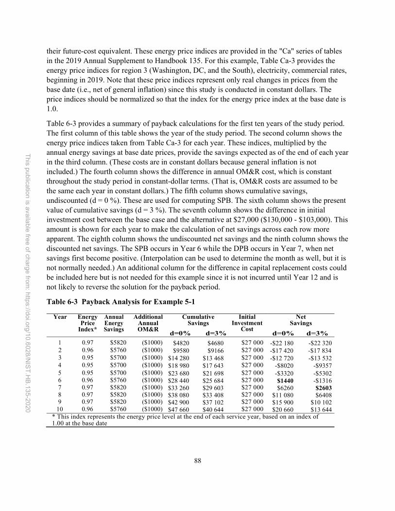
88

This p

ublica

tion is ava

ilab

le free

of ch

arge

from: h

ttps://doi.o

rg/1

0.6

028

/NIS

T.H

B.13

5-202

0

their future-cost equivalent. These energy price indices are provided in the "Ca" series of tables in the 2019 Annual Supplement to Handbook 135. For this example, Table Ca-3 provides the energy price indices for region 3 (Washington, DC, and the South), electricity, commercial rates, beginning in 2019. Note that these price indices represent only real changes in prices from the base date (i.e., net of general inflation) since this study is conducted in constant dollars. The price indices should be normalized so that the index for the energy price index at the base date is 1.0.

Table 6-3 provides a summary of payback calculations for the first ten years of the study period. The first column of this table shows the year of the study period. The second column shows the energy price indices taken from Table Ca-3 for each year. These indices, multiplied by the annual energy savings at base date prices, provide the savings expected as of the end of each year in the third column. (These costs are in constant dollars because general inflation is not included.) The fourth column shows the difference in annual OM&R cost, which is constant throughout the study period in constant-dollar terms. (That is, OM&R costs are assumed to be the same each year in constant dollars.) The fifth column shows cumulative savings, undiscounted (d = 0 %). These are used for computing SPB. The sixth column shows the present value of cumulative savings (d = 3 %). The seventh column shows the difference in initial investment cost between the base case and the alternative at $27,000 ($130,000 - $103,000). This amount is shown for each year to make the calculation of net savings across each row more apparent. The eighth column shows the undiscounted net savings and the ninth column shows the discounted net savings. The SPB occurs in Year 6 while the DPB occurs in Year 7, when net savings first become positive. (Interpolation can be used to determine the month as well, but it is not normally needed.) An additional column for the difference in capital replacement costs could be included here but is not needed for this example since it is not incurred until Year 12 and is not likely to reverse the solution for the payback period.

Table 6-3 Payback Analysis for Example 5-1

Year Energy Price

Index*

Annual Energy Savings

Additional Annual OM&R

Cumulative Savings

Initial Investment

Cost

Net Savings

d=0% d=3% d=0% d=3%

1 0.97 $5820 ($1000) $4820 $4680 $27 000 -$22 180 -$22 320 2 0.96 $5760 ($1000) $9580 $9166 $27 000 -$17 420 -$17 834 3 0.95 $5700 ($1000) $14 280 $13 468 $27 000 -$12 720 -$13 532 4 0.95 $5700 ($1000) $18 980 $17 643 $27 000 -$8020 -$9357 5 0.95 $5700 ($1000) $23 680 $21 698 $27 000 -$3320 -$5302 6 0.96 $5760 ($1000) $28 440 $25 684 $27 000 $1440 -$1316 7 0.97 $5820 ($1000) $33 260 $29 603 $27 000 $6260 $2603 8 0.97 $5820 ($1000) $38 080 $33 408 $27 000 $11 080 $6408 9 0.97 $5820 ($1000) $42 900 $37 102 $27 000 $15 900 $10 102

10 0.96 $5760 ($1000) $47 660 $40 644 $27 000 $20 660 $13 644 * This index represents the energy price level at the end of each service year, based on an index of 1.00 at the base date

89

This p

ublica

tion is ava

ilab

le free

of ch

arge

from: h

ttps://doi.o

rg/1

0.6

028

/NIS

T.H

B.13

5-202

0

6.4.4 Alternative SPB Computations

In the limited case where ΔEt, ΔWt, and ΔOMRt are assumed to be the same in every year (i.e., there is no price escalation and quantities of energy and water saved each year are the same) and there are no additional non-annually recurring OM&R or replacement costs or other costs, the SPB can be computed as follows:

𝑆𝑃𝐵 =∆𝐼

∆𝐸 + ∆𝑊 + ∆𝑂𝑀𝑅(6 − 13)

Equation 6-13 is often used in practice. As a screening tool for qualifying projects that are clearly cost effective, this is acceptable. Applying this simplified SPB formula to Example 5-1, we get a SPB of 5.4 years for the energy-conserving HVAC alternative.

𝑆𝑃𝐵 =130 000 − 103 000

(30 000 − 24 000) + (7000 − 8000)= 5.4 (6 − 14)

Since the additional replacement cost does not occur until Year 12 and there is little difference in the residual value at the end of the 20-year life of both systems, an SPB in Year 6 of a 20-year study period is a strong indication that the project alternative is cost effective and may not warrant further economic analysis unless it is competing with other projects for limited investment funding.

6.4.5 Summary of Payback Methods

• SPB and DPB measure how long it takes to recover initial investment costs. • DBP includes the time-value of money in the calculation. • Payback is useful only as a rough guide for accept/reject decisions and is not recommended as

a criterion for selecting among mutually exclusive alternatives or for ranking independent projects.

90

This p

ublica

tion is ava

ilab

le free

of ch

arge

from: h

ttps://doi.o

rg/1

0.6

028

/NIS

T.H

B.13

5-202

0

7 Applying LCC Measures to Project Investments

The previous chapters of this handbook were devoted to the mechanics of LCCA and the special requirements of the FEMP rules in 10 CFR 436 for economic analysis of energy and water conservation projects in federal facilities. This chapter shows how to apply LCCA and supplementary economic measures (i.e., NS, SIR, and AIRR) to different types of investment decisions related to these projects.

Five types of capital investment decisions frequently encountered in evaluations of energy and water conservation projects are identified in Chapter 2:

(1) Accept or reject a single project or system option (2) Select an optimal efficiency level for a building system (3) Select an optimal system type from competing alternatives (4) Select an optimal combination of interdependent systems (5) Rank independent projects to allocate a limited capital investment budget

The term "optimal," as used here, means the most cost-effective choice from available alternatives; it does not refer to technical performance and does not include project alternatives that are not available at the required time and place. The first four of these investment decisions are similar in that they all involve the evaluation of mutually exclusive alternatives. That is, of the two or more choices being considered (even an accept/reject decision must have a base case for comparison), only one alternative can be selected. The fourth decision involves the simultaneous analysis of two or more interdependent systems, where each system has two or more mutually exclusive alternatives. These first four decision types identify the most cost-effective project alternative(s) in the sense that they minimize life-cycle costs. However, they do not address the problem of a budget constraint: that is, how do you allocate a limited capital investment budget among several independent (competing) projects to maximize the effectiveness of that budget. This is the domain of the fifth decision type. Table 2-1 in Chapter 2 provides examples for each of these decision types.

7.1 Accept or Reject a Single Project Alternative

An accept/reject decision relates to the economic evaluation of a project having a single design or system option that you are considering for purchase. No competing alternatives are considered in this analysis (although it is usually advisable to consider other alternatives). You will either accept this project or reject it, depending on its cost-effectiveness. Examples might include the decision to

• install storm windows over existing single-pane windows, • install an air-lock door in a building entryway, or • replace an electric water heater with a gas-fired model.

Even a single project alternative must be evaluated against a base case. The base case for a single project alternative is generally the "do-nothing" alternative. This base case will typically have no initial investment cost, but higher operational (e.g., energy, water, or OM&R) costs than the

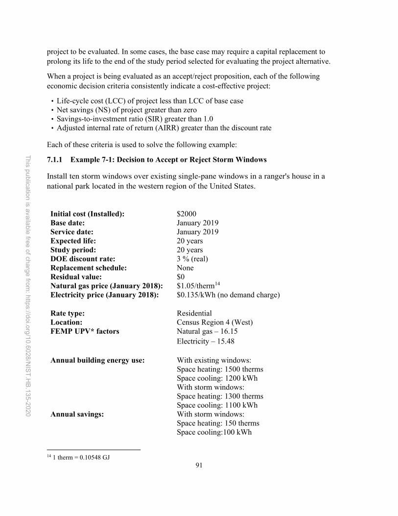
91

This p

ublica

tion is ava

ilab

le free

of ch

arge

from: h

ttps://doi.o

rg/1

0.6

028

/NIS

T.H

B.13

5-202

0

project to be evaluated. In some cases, the base case may require a capital replacement to prolong its life to the end of the study period selected for evaluating the project alternative.

When a project is being evaluated as an accept/reject proposition, each of the following economic decision criteria consistently indicate a cost-effective project:

• Life-cycle cost (LCC) of project less than LCC of base case • Net savings (NS) of project greater than zero • Savings-to-investment ratio (SIR) greater than 1.0 • Adjusted internal rate of return (AIRR) greater than the discount rate

Each of these criteria is used to solve the following example:

7.1.1 Example 7-1: Decision to Accept or Reject Storm Windows

Install ten storm windows over existing single-pane windows in a ranger's house in a national park located in the western region of the United States.

Initial cost (Installed): $2000 Base date: January 2019 Service date: January 2019 Expected life: 20 years Study period: 20 years DOE discount rate: 3 % (real) Replacement schedule: None Residual value: $0 Natural gas price (January 2018): $1.05/therm14 Electricity price (January 2018): $0.135/kWh (no demand charge)

Rate type: Residential Location: Census Region 4 (West) FEMP UPV* factors Natural gas – 16.15 Electricity – 15.48 Annual building energy use: With existing windows: Space heating: 1500 therms Space cooling: 1200 kWh With storm windows: Space heating: 1300 therms Space cooling: 1100 kWh Annual savings: With storm windows: Space heating: 150 therms Space cooling:100 kWh

14 1 therm = 0.10548 GJ

92

This p

ublica

tion is ava

ilab

le free

of ch

arge

from: h

ttps://doi.o

rg/1

0.6

028

/NIS

T.H

B.13

5-202

0

Additional considerations:

Additional window washing requirements will be performed by occupants as a housekeeping chore at no additional cost to government. Occupant comfort on cold days will be improved.

7.1.1.1 LCC Solution

The LCC formula can be used to solve this accept/reject investment problem. This formula (based on Equation 5-2) is applied to both the base case and the alternative to determine which has the lower LCC.

𝐿𝐶𝐶 = I + Repl − Res + E + OMR + X (7 − 1) where:

LCC = Total LCC in present-value dollars of a given alternative I0 = Initial investment costs

Repl = Present-value capital replacement costs Res = Present-value residual value (resale value, scrap value, salvage value) less

disposal costs E = Present-value energy costs OMR = Present-value non-fuel operating, maintenance, and repair costs X = Present-value other costs

LCC solution for "do-nothing" base case (do not install storm windows):

I0 = 0

Repl = 0 Res = 0 E = 1.05 * 1500 therms * 16.15 + 0.135 * 1200 kWh * 15.48 OMR = 0 X = 0

Total LCC = $27 944

LCC solution for alternative (install storm windows):

I0 = 2000

Repl = 0 Res = 0 E = 1.05 * 1300 therms * 16.15 + 0.135 * 1100 kWh * 15.48 OMR = 0 X = 0

Total LCC = $2000 + $24 344 = $26 344

Conclusion: The LCC for storm windows ($26 344) is lower than the LCC for existing windows ($27 944); installing storm windows is cost effective and should be accepted.

7.1.1.2 NS Solution

93

This p

ublica

tion is ava

ilab

le free

of ch

arge

from: h

ttps://doi.o

rg/1

0.6

028

/NIS

T.H

B.13

5-202

0

This accept/reject problem can also be solved by using the NS method. The NS is a measure of the expected long-run profitability of the project to be undertaken. You can calculate the NS by simply taking the difference between the LCC of the base case (do not install storm windows) and the LCC of the alternative (install storm windows): $27 944 - $26 344 = $1600.

However, for this example we will use the NS formula for building-related projects presented in Section 6.1.2 (Equation 6-2). This helps us set up the same problem for solution with SIR and AIRR in the next sections.

𝑁𝑆 : = [∆𝐸 + ∆𝑂𝑀𝑅 + ∆𝑋] − [∆𝐼 + ∆𝑅𝑒𝑝𝑙 − ∆𝑅𝑉] (7 − 2)

Where: 𝑁𝑆 : = Net savings, operation-related savings minus additional investment costs

for alternative (A) relative to base case (BC) ΔE = (𝐸 − 𝐸 ) Savings in energy costs attributable to the alternative

ΔOMR = 𝑂𝑀𝑅 − 𝑂𝑀𝑅 Savings in OM&R costs attributable to the alternative ΔX = 𝑋 − 𝑋 Savings in other costs attributable to the alternative Δ𝐼 = 𝐼 − 𝐼 Additional initial investment cost required for



ΔE = (𝐸 − 𝐸 ) $1.05/therm * 200 therms * 16.15 + $0.135/kWh *

100 kWh * 15.48 = $3600

Δ𝐼 = 𝐼 − 𝐼 $2000

Conclusion: After discounting all costs to present value, net savings ($1600 in present-value terms) is positive; the storm windows are cost-effective.

7.1.1.3 SIR Solution

The SIR method can also be used to determine whether to accept or reject the storm window investment. It expresses the savings that can be achieved for each dollar invested in the energy-saving alternative. The SIR must be greater than 1.0 for the storm windows to generate more savings than costs. In this calculation we use the SIR formula for building-related projects as presented in Section 6.2.2 (Equation 6-4):

𝑆𝐼𝑅 : =∆𝐸 + ∆𝑂𝑀𝑅 + ∆𝑋

∆𝐼 + ∆𝑅𝑒𝑝𝑙 − ∆𝑅𝑉=

$3600

$2000= 1.80

(7 − 3)

94

This p

ublica

tion is ava

ilab

le free

of ch

arge

from: h

ttps://doi.o

rg/1

0.6

028

/NIS

T.H

B.13

5-202

0

Conclusion: The storm windows' SIR of 1.80 passes the test for cost-effectiveness. For each one dollar invested in the storm windows, $1.80 will be saved, over and above the 3 % discount rate reflecting the minimum acceptable rate of return.

7.1.1.4 AIRR Solution

The AIRR method can be used to evaluate the cost-effectiveness of the storm windows when you are interested in a measure of project yield annually. If the AIRR for the storm windows is greater than the required rate of return (as reflected in the 3 % discount rate in our example), it indicates that the annual yield of the energy-saving project exceeds that of the next best opportunity for investing your funds. The simplified formula for computing the AIRR, as presented in Section 6.3.1 (Equation 6-6), is used here to compute the AIRR of the storm windows.

𝐴𝐼𝑅𝑅 = (1 + 𝑟) ∙ (𝑆𝐼𝑅) − 1

= (1 + 0.03) ∙ (1.80) − 1= 0.0607

𝐴𝐼𝑅𝑅 ≈ 6.1 % (7 − 4)

Conclusion: The AIRR of 6.1 % (real) for the storm windows is greater than the real discount rate of 3.0 %. The AIRR solution shows that the storm windows are cost-effective, consistent with the results of the LCC, NS, and SIR analyses.

7.2 Select Optimal Efficiency Level

The optimal efficiency level refers to the problem of selecting the most cost-effective level of energy performance (or other scalable performance parameter – water, sustainability, resilience) for a building system. "Efficiency level" here means achieving a certain level of performance outcome (e.g., maintain a building’s thermal conditions) with different amounts of resource input (e.g., energy); the lower the input requirement, the higher the efficiency. The energy efficiency of a building system can vary over a wide range while producing approximately the same level of thermal comfort, convenience, or lumens. Good examples of this type of decision include the selection of

• the level of insulation to be installed in a roof, wall, or floor of a building, • the level of thermal performance for window systems, • the efficiency of heating or cooling equipment, or • the rated capacity area of a solar photovoltaic system.

Generally, we can assume that the more efficient the system, the higher its investment cost. This type of decision is different from the accept/reject decision shown above because the object is not to determine whether an efficiency level is cost-effective. Instead, the objective is to determine which of the available efficiency levels is the most cost-effective for the application being considered.

95

This p

ublica

tion is ava

ilab

le free

of ch

arge

from: h

ttps://doi.o

rg/1

0.6

028

/NIS

T.H

B.13

5-202

0

Consider the case of thermal insulation in the exterior envelope of a building. Insulation can generally be installed over a wide range of R-values (thermal resistance values), and in general the higher the R-value the lower the energy loss (or gain). However, these savings are subject to diminishing marginal returns; that is, each additional unit saves less than the one before. While the first units may be cost effective, beyond some point it no longer pays to install additional insulation.

The optimal energy efficiency level for a building system, whether roof, walls, windows, lighting, or heating and cooling equipment, is generally the level that minimizes LCC or maximizes net savings. Both measures will give an identical solution if applied properly. Do not use the SIR, AIRR, or payback measures to determine this solution. The efficiency level with the highest SIR or AIRR (or shortest payback) will not be the economically optimal level. The SIR and AIRR measures usually decline with each additional unit of efficiency, since the additional energy savings generated tend to decline with each unit increase in efficiency.

7.2.1 Example 7-2: Decision on Optimal Level of Insulation

This example illustrates the computation of LCC and NS measures to determine the optimal R-value of attic insulation to be installed in a new low-rise residential building on a military base in Ohio. The key dates and assumptions are as follows:

Base Date: January 2019 Service Date: January 2019 Expected Life: 25 years Study Period: 25 years DOE Discount Rate: 3 % (real) Replacement Schedule: None Residual Value: $0 Electricity Price (January 2018): $0.10/kWh (no demand charge) Rate Type of Energy: Residential Location: Ohio - Census Region 2 (Midwest) FEMP UPV* Factor - Electricity 17.53

Six different levels of cellulose insulation are being considered, ranging from R-30 to R-80 in increments of R-10. Note that the optimal R-value for any given building is determined by numerous factors, including climate, fuel prices, the efficiency and operating schedule of the heating and cooling equipment, the incremental cost of each level of insulation considered, and the study period and discount rate selected for the analysis.

Table 7-1 shows the initial cost and annual electricity usage for space heating and cooling for each R-value being evaluated. The annual per kWh cost is found by multiplying the annual electricity usage by the unit cost at the base date price ($0.10/kWh). Life-cycle energy costs, in present-value dollars, are found by multiplying the annual electricity cost by the FEMP UPV* factor for electricity in Census Region 2. (This factor is taken from Table Ba-2 of the 2019

96

This p

ublica

tion is ava

ilab

le free

of ch

arge

from: h

ttps://doi.o

rg/1

0.6

028

/NIS

T.H

B.13

5-202

0

Annual Supplement to Handbook 135) The LCC is the sum of initial cost and present-value energy costs over the study period.

R-60 has the lowest LCC ($15 824) and the highest net savings ($1706) in this example. Thus R-60 is the economically optimal R-value for this application. Note that for other energy types or prices, or for a different set of heating and cooling requirements, the optimal R-value may be different. Table 7-1 shows the SIR for each level of insulation relative to the R-0 level. Note that the R-value with the highest SIR (R-50) is NOT the level of insulation with the lowest LCC.

Table 7-1 Payback Analysis for Example 5-1

R-Value Initial Cost

Annual kWh

Energy Cost Total PV LCC

Net Savings

SIR

Annual Life (PV)R-0 $0 10 000 $1000 $17 530 $17 530 $0 N/A

R-30 $900 9200 $920 $16 128 $17 028 $502 1.56 R-40 $1200 8600 $860 $15 076 $16 276 $1254 2.05 R-50 $1500 8200 $820 $14 375 $15 875 $1655 2.10 R-60 $1800 8000 $800 $14 024 $15 824 $1706 1.95 R-70 $2100 7900 $790 $13 849 $15 949 $1581 1.75 R-80 $2400 7850 $785 $13 761 $16 161 $1369 1.57

One of the advantages of using the LCC method for solving the optimal-efficiency problem is that you do not have to identify a base case. Whether or not the R-0 is included in the analysis, the LCC of each of the other R-values will be the same. One of the advantages of using the net savings method is that you do not need to know the total annual energy usage for space heating and cooling; you can use the annual energy savings. But with the NS method you must identify a base case from which the energy savings are referenced; in our example the base case is the R-0 level.

7.3 Select Optimal System Type

Optimal system selection refers to the problem of selecting the most cost-effective system type for an application. Examples of this investment decision category include

• selection of the heating system type (e.g., electric resistance, gas base board, heat pump), • selection of wall construction type (e.g., masonry, wood frame, or curtain wall), or • selection of water heater type to be installed in a new building (e.g., gas, electric, solar).

The choice of system type may affect the energy use of the building, but the amount of energy used is sometimes not a primary consideration in the selection. For example, the choice between concrete-masonry construction and curtain wall construction for exterior walls of an office building may be dictated more by long-term maintenance costs and fire safety than by energy usage, but that choice will affect the heat loss and heat gain through the wall. The choice of fuel

97

This p

ublica

tion is ava

ilab

le free

of ch

arge

from: h

ttps://doi.o

rg/1

0.6

028

/NIS

T.H

B.13

5-202

0

type for space heating also falls into this category, since it is not simply a matter of fuel utilization efficiency but of cost-effectiveness in the application that is to be considered.

7.3.1 Example 7-3: Selection of Optimal Type of HVAC System

In Example 7-3 we look at five different types of heating/cooling systems being considered for installation in a house on a military base in New York State. The key dates and assumptions are as follows:

Base date: January 2019 Service date: January 2019 Expected life: 15 years Study period: 15 years DOE discount rate: 3 % (real) Replacement schedule: None Residual value: $0 Electricity price (January 2018): $0.18/kWh (no demand charge) Rate type of energy: Residential Location: New York Census Region 1 (Northeast) UPV factor (OM&R costs): 11.938 Annual space heating load: 52.75 GJ (~ 50 MMBtu) Annual space cooling load: 21.10 GJ (~ 20 MMBtu) Fuel prices as of base date: Electricity: $50.00/GJ ($0.18/kWh) Fuel Oil: $22.74/GJ ($3.40/Gal) LPG: $21.40/GJ ($3.20/Gal) Natural Gas: $10.97/GJ ($1.16/therm) FEMP UPV* Factors Electricity: 13.07 Fuel Oil: 13.94 LPG: 15.86 Natural Gas: 13.75

Four different fuel types are available at the site: electricity, fuel oil (distillate), LPG, and natural gas. The costs are converted to a common unit ($/GJ) to simplify the analysis for the reader. We can assume that the optimal energy utilization efficiency for each system type (i.e., the efficiency level with the lowest LCC) has already been determined before making the decision as to which system type is most cost-effective for this house. To make this problem easier, each system is assumed to have the same expected life (15 years). The optimal heating/cooling system will depend on the annual space heating and cooling requirements, price per GJ of fuel, seasonal efficiency of each system, OM&R costs, study period, and discount rate.

Table 7-2 shows, for five different HVAC system alternatives, the system-specific data needed for computing annual energy usage and life-cycle costs: initial costs, annual OM&R costs, and seasonal efficiency. Initial costs are lowest for the electric baseboard system with window air

98

This p

ublica

tion is ava

ilab

le free

of ch

arge

from: h

ttps://doi.o

rg/1

0.6

028

/NIS

T.H

B.13

5-202

0

conditioner (AC) and highest for the natural gas furnace with a central AC. The cost of the fuel oil and LPG furnaces include a storage tank. The cost of the natural gas furnace includes the installation of a pipeline from the street. Efficiency is the number of units of energy transfer resulting from one unit of energy input. Electric heating converts 100 % of energy input into energy transferred for heating. Fuels combusted on-site (fuel oil, liquefied petroleum gas, and natural gas) have efficiencies below 1.0. Heat pumps are the most efficient because more than one unit of energy can be transferred per unit of energy input. The heat pump has the highest OM&R costs while the electric baseboard/window AC system has the lowest.

Table 7-2 System Types, Costs, and Seasonal Efficiency Data for Example 7-3

System Type Initial Cost ($)

Annual OM&R Cost ($)

Heating Efficiency /

COP Electric Baseboard / Window AC 4500 75 1.00 / 3.0 Heat Pump (Central) 6000 200 2.00 / 3.0 Oil Furnace / Central AC 6500 125 0.82 / 3.0 LPG Furnace / Central AC 6500 100 0.85 / 3.0 Natural Gas Furnace / Central AC 7000 100 0.85 / 3.0

Table 7-3 shows the LCC solution for each of the five systems. The cost of cooling is the same across all systems because all use electricity and have the same cooling efficiency (3.0 COP). The following is the calculation of cooling cost: (21.10 GJ of cooling load) / (3.0 efficiency) * ($50/GJ of electricity). Therefore, the differences in energy costs are driven by the different heating technologies. The following is the calculation of heating cost: (52.75 GJ of heating load) / (efficiency) * ($/GJ for fuel).

Table 7-3 Present-Value Costs, LCC and NS Solutions for Example 7-3

Present Value Costs ($) LCC NS SIR System Type Initial OM&R Energy ($) ($) ($)

Electric Baseboard / Window AC 4500 895 39 068 44 463 N/A N/A Heat Pump (Central) 6000 2388 21 832 30 220 14 243 9.50 Oil Furnace / Central AC 6500 1492 24 988 32 980 11 483 5.74 LPG Furnace / Central AC 6500 1194 25 659 33 353 11 110 5.56 Natural Gas Furnace / Central AC 7000 1194 13 957 22 151 22 312 8.92

In this example the natural gas furnace/central AC has the lowest LCC ($22 151) and highest net savings ($22 312) of the five systems and is, therefore, the most cost-effective system choice for this specific application. Note, however, that it does not have the highest SIR. The heat pump, which ranks second in terms of LCC, has the highest SIR (9.50). This example emphasizes that

99

This p

ublica

tion is ava

ilab

le free

of ch

arge

from: h

ttps://doi.o

rg/1

0.6

028

/NIS

T.H

B.13

5-202

0

the SIR is not a valid method for determining the HVAC system with the lowest LCC. The energy costs over the study period are by far the biggest driver of the LCC results. Since natural gas is the cheapest fuel type, it is reasonable to expect it to be one of, if not the, lowest life-cycle cost option.

7.4 Select Optimal Combination of Interdependent Systems

Determining the optimal design or energy efficiency for several interdependent systems within a facility generally requires a simultaneous energy analysis to properly account for the interaction among the systems. This interaction occurs when the use of one system affects the energy use of other systems in the same facility. For example, as the thermal performance of a building envelope increases (i.e., more insulation and more efficient window systems reduce thermal transfer), the energy savings from efficiency improvements to the heating/cooling system diminish (i.e., lower thermal loads decrease heating/cooling operation), making the latter improvements less cost-effective. Similarly, as the efficiency of the heating/cooling system is increased, the energy savings from adding insulation and more efficient windows diminish, making these less cost-effective as well.

Building system interactions that are most likely to have an impact on energy savings are those related to

• HVAC system efficiency, • the thermal integrity of the overall building envelope, and • lighting system efficiency and usage.

Interactions among the various envelope components themselves (including windows, walls, and roof) are less important, difficult to measure, and difficult to document. The time to pay most attention to system interactions is during the design phase of a new building. Retrofit projects in an existing building are usually more restrictive in terms of the number of systems that can be substantially modified at the same time.

Simultaneous analysis of several building systems requires a whole-building energy analysis (using a building energy simulation program such as EnergyPlus) for each combination of system specifications to be evaluated. The calculated energy usage for the whole building reflects the interaction of these building systems. The difference in building energy usage from one combination of system specifications to another is the savings attributable to all changes. There is no need to estimate savings attributable to individual systems or conservation measures when performing this analysis. Some whole-building energy analysis programs can be set up in a parametric mode that automatically changes one or more system parameters incrementally (e.g., R-value of wall insulation or heating system efficiency) with each run.

While whole-building energy analysis is not conceptually difficult, the number of potential system combinations to be evaluated can be very large and unwieldy. In general, only practical and balanced combinations of alternatives need to be considered. Thus, it is unlikely that a low level of roof insulation and a high-efficiency window glazing would be used together. Unlikely

100

This p

ublica

tion is ava

ilab

le free

of ch

arge

from: h

ttps://doi.o

rg/1

0.6

028

/NIS

T.H

B.13

5-202

0

system combinations should be eliminated to the extent possible before performing an energy analysis on the remaining combinations.

Once the energy usage of each combination of systems is estimated, an LCCA can be performed for each combination of system specifications. This LCC is based on the total initial investment costs, replacement costs, residual values, and OM&R costs for each combination of systems being evaluated, and the corresponding energy usage for that combination (all in present value terms). The most cost-effective combination of building system specifications is the combination with the overall lowest LCC.

7.4.1 Example 7-4: Selection of Optimal Combination of Thermal Envelope and HVAC System Efficiency

This example shows an LCCA for a hypothetical administration building being designed for a West Coast location. Five different levels of thermal efficiency (i.e., resistance to heat loss and heat gain) in the envelope system (E1 through E5), and three different levels of HVAC energy conversion efficiency (H1 through H3) are being considered for this building. Higher levels of efficiency have higher initial costs (Table 7-4) but use less energy than lower levels (Table 7-5). Two energy types are assumed, natural gas for heating and electricity for cooling and fan operation. Since the envelope and HVAC systems are interdependent from an energy usage standpoint, the energy analysis must be performed for the entire building rather than for the individual systems. The design objective in this example is to determine which envelope and HVAC system combination results in the lowest LCC.

The basic economic and technical assumptions needed for this analysis are as follows:

Base Date: January 2019 Service Date: January 2019 Expected Life: 25 years Study Period: 25 years DOE Discount Rate: 3 % (real) Replacement Schedule: None Residual Value: $0 Electricity Price (January 2018): $0.165/kWh (no demand charge) Rate Type of Energy: Residential Location: Pacific contiguous Census Region 4 (West) UPV Factor (OM&R Costs): 17.413 Fuel Prices as of Base Date: Electricity: $45.83/GJ ($0.165/kWh) Natural Gas: $21.70/GJ ($1.21/therm) FEMP UPV* Factors Electricity: 18.40 Natural Gas: 19.27

101

This p

ublica

tion is ava

ilab

le free

of ch

arge

from: h

ttps://doi.o

rg/1

0.6

028

/NIS

T.H

B.13

5-202

0

Table 7-4 Initial Cost of Envelope and HVAC Systems for Example 7-4

Envelope System

Initial Cost ($)

HVAC System

Initial Cost ($)

E1 0 H1 0 E2 10 000 H2 30 000 E3 21 000 H3 74 000 E4 44 000 E5 80 000

Table 7-5 Annual Energy Usage by Envelope and HVAC System Alternative for Example 7-4

Natural Gas (GJ) HVAC System

Envelope System H1 H2 H3

E1 1285 1124 1058 E2 1221 1068 1005 E3 1163 998 958 E4 1112 973 915 E5 1000 933 878

Electricity (GJ) HVAC System


E1 350 300 266 E2 332 285 253 E3 318 272 242 E4 306 262 233 E5 298 255 226

Each level of envelope efficiency shown builds on the previous level, increasing the initial investment cost of the building but reducing annual heating and cooling requirements. Likewise, each HVAC system alternative shown has a higher initial investment cost but reduces the energy needed to satisfy a given heating and cooling load. The base level for both the envelope and the HVAC equipment is shown to have zero initial cost because it is assumed that these represent minimum acceptable levels of performance. Only investment costs above these minimum levels of performance are needed for this analysis. To make the problem easier to demonstrate, OM&R costs are assumed to be the same for each level of envelope efficiency and each level of HVAC system efficiency, no replacements are needed during the 25-year study period, and the residual value of each alternative is assumed to be zero (note that all of these are plausible assumptions, given the technologies involved). In addition, the potential reduction in the initial cost of the HVAC system due to a downsizing of maximum heating and cooling loads is also assumed to be negligible. Thus, the LCC shown here is simply the sum of the initial cost of the envelope and

102

This p

ublica

tion is ava

ilab

le free

of ch

arge

from: h

ttps://doi.o

rg/1

0.6

028

/NIS

T.H

B.13

5-202

0

system improvements plus the present value of natural gas and electricity costs for space heating and cooling. For example, the LCC of the combination E2 and H3 can be computed as follows:

LCCE2,H3 = $10 000 (initial cost of E2)

+ $74 000 (initial cost of H3) + 1005 GJ * $21.70/GJ * 19.27 (PV cost of natural gas) + 253 GJ * $45.83/GJ * 18.40 (PV cost of electricity) = 10 000 + 74 000 + 420 250 + 213 348 = $717 598

The LCC for each envelope and HVAC system combination from Example 7-4 is shown in Table 7-6. The first column shows LCC calculations for each of the five thermal envelope alternatives, given the base-level HVAC system. If the base-level HVAC system (H1) were to be selected, the most cost-effective envelope alternative would be E4, with an LCC of $749 454. If HVAC system H3 were to be selected, the most cost-effective envelope alternative would be E4, with a total LCC of $697 098. If the base-level thermal envelope E1 were selected, the most cost-effective HVAC system would be H3, with an LCC of $740 723. But if E5 were selected, the most cost-effective HVAC system would be H3 with an LCC of $711 723. The combination with the lowest LCC ($697 098) is E4,H3 (bold).

Table 7-6 LCC Solution for Selecting the Optimal Combination of Building Envelope and HVAC System for Example 7-4

LCC HVAC System


E1 $832 480 $752 992 $740 723 E2 $800 538 $726 926 $717 598 E3 $775 479 $697 693 $699 668 E4 $767 034 $701 806 $697 098 E5 $749 454 $715 177 $711 723

The LCC method is the most appropriate method for evaluating interactive system combinations. The net savings measure can also be used to determine the optimal combination; the combination with the highest NS is the same as the combination with the lowest LCC. However, in order to compute the NS, a base case system combination must be identified first (e.g., E1,H1 in this example) and the NS for each combination to be evaluated must be computed with respect to that base case. The choice of the combination with the highest SIR and AIRR, or the shortest Payback, will not yield the correct combination in most cases.

In this example the difference in the LCC for some combinations close to the optimal combination (E4,H3) is relatively small. The determination of the optimal combination is likely to be quite sensitive to uncertain parameters such as OM&R costs or future energy costs. Thus, fine

103

This p

ublica

tion is ava

ilab

le free

of ch

arge

from: h

ttps://doi.o

rg/1

0.6

028

/NIS

T.H

B.13

5-202

0

tuning of this method by examining large numbers of potential combinations of interdependent systems is probably not warranted either from a design cost or LCC standpoint. Still it is important to recognize that the interaction among building systems can affect the economics of design choices and to understand how to take these considerations into account.

7.5 Rank Independent Projects for Funding Allocation

Up to this point, this chapter has shown how LCC and related measures of economic analysis can be used to determine cost-effective choices among mutually exclusive project alternatives. These are applications where only one alternative for any given system is to be selected. This section addresses the use of economic analysis to rank two or more independent projects - all of which have already been shown to be cost-effective - to allocate limited funding. Independent projects are projects that can be implemented in the same or different buildings without significantly affecting the cost effectiveness of one another.

Since all the independent projects being considered have already been identified as cost-effective, it would generally be advantageous to implement them all. However, there may be insufficient investment funding for this purpose and it is therefore important that the funding available be allocated to achieve the greatest overall net savings. The FEMP LCC rules require the use of either the SIR or AIRR measures for establishing priority for ranking independent projects. Projects are ranked in order of SIR or AIRR and funded in descending rank order until the available funding runs out (the same results will be achieved by using either the SIR or AIRR for ranking projects). If additional funding is made available later, it will be allocated to the remaining projects (and any new projects introduced in the interim) using this same criterion. In the remainder of this section, only the SIR method will be demonstrated.

Note that only the SIR and AIRR measures provide an acceptable method for ranking independent projects for funding purposes. Do not use the LCC, NS, or payback measures for individual projects as a means of ranking them with other independent projects.

If several interdependent projects have been identified for potential funding, these are best evaluated by combining them into a single project with a combined SIR and ranking this project along with other independent projects. The information on individual projects within a set should be preserved to allow selections from the set when budget limitations preclude funding all projects within a set.

A practical advantage of using the SIR measure for ranking independent projects is that the same study period is not required for each project, as it is when evaluating mutually exclusive projects. This is especially important when projects are submitted by different analysts or for different buildings. For example, if new roof insulation in one building is evaluated with a study period of 25 years and a new computer control system for HVAC equipment in a different building is evaluated with a study period of 15 years, the two projects can still be ranked by their individual SIRs when allocating funding. This advantage is based on the implicit assumption that any project can be replicated (i.e., replaced with a similar system having similar costs and savings) at the end of its life. However, when calculating SIRs for ranking independent projects, do not

104

This p

ublica

tion is ava

ilab

le free

of ch

arge

from: h

ttps://doi.o

rg/1

0.6

028

/NIS

T.H

B.13

5-202

0

include project replication in the analysis (i.e., do not include project replacements to force a longer life).

If an SIR is calculated when performing an analysis of mutually exclusive alternatives for a given project (although it is not necessary for that analysis), the resulting SIR may not be appropriate for ranking that project with respect to other independent projects. If the project analysis included capital replacements to force a common study period, the project's SIR will need to be recalculated without the replacements before it can be used for project ranking.

7.5.1 Example 7-5: Simple SIR Ranking

Table 7-7 demonstrates the most straightforward application of the SIR ranking method. Six independent conservation projects are proposed for funding, but only $700 000 is available for funding conservation projects this year. All six projects have already been shown to be cost-effective relative to their corresponding base cases in that they have an SIR greater than 1.0 and NS greater than zero. If $1 600 000 were available to fund these projects, all six could be funded at a present-value NS of $3 800 000.

Table 7-7 NS Solutions for Selecting Best Project Mix Given Budget Limit

Initial Cost Total Savings SIR

Net Savings Cumulative Investment

Cumulative Net Savings

Project ($) ($) ($) ($) ($)

A 100 000 1 000 000 10.0 900 000 100 000 900 000 F 100 000 500 000 5.0 400 000 200 000 1 300 000 E 200 000 800 000 4.0 600 000 400 000 1 900 000 C 300 000 10 00000 3.3 700 000 700 000 2 600 000 B 500 000 15 00000 3.0 1 000 000 1 200 000 3 600 000 D 400 000 600 000 1.5 200 000 1 600 000 3 800 000

The projects are listed in Table 7-7 in declining order of their SIR. The column labeled "Cumulative Investment" indicates how far down the list the $700 000 funding will reach. Projects A, F, E, and C will be funded with a cumulative NS of $2 600 000. No other combination of projects from this list that can fit into the $700 000 budget constraint can produce greater cumulative NS.

7.5.2 Example 7-6: SIR Ranking of Individual Projects

In Example 7-5 the top four projects, as ranked by SIR, fit exactly into the available capital investment budget. This may not always be the case. Table 7-8 shows eight independent projects that together have a total investment cost of $2 750 000. However, only $1 200 000 in capital funding is available this year.

105

This p

ublica

tion is ava

ilab

le free

of ch

arge

from: h

ttps://doi.o

rg/1

0.6

028

/NIS

T.H

B.13

5-202

0

Table 7-8 Present-Value Costs, LCC and NS Solutions for Selecting Optimal Type of HVAC System for Example 7-3

Project Initial Cost Total Savings Net Savings SIR

($) ($) ($)

A 300 000 400 000 100 000 1.33 B 200 000 1 000 000 800 000 5.00 C 200 000 600 000 400 000 3.00 D 250 000 600 000 350 000 2.40 E 300 000 450 000 150 000 1.50 F 100 000 280 000 180 000 2.80 G 400 000 700 000 300 000 1.75 H 1 000 000 2 000 000 1 000 000 2.00

Table 7-9 reorganizes the projects in descending order using SIR. The projects are funded in declining order of SIR. But when project H (ranked 5th with an SIR of 2.0 and an initial cost of $1 000 000) is reached, it cannot be funded within the remaining funding of $450 000 ($1 200 000 - $750 000). If project H is divisible into smaller parts, each having the same SIR, then the remaining $450 000 should be invested in that project. But if H cannot be divided up, the solution to this problem becomes more complex. Project H should be skipped over for now, and project G, at $400 000, should be included. This leaves $50 000 un-invested if no other project can be broken down into smaller pieces.


Project Initial Cost Total Savings

Net Savings SIR BCDFG Cumulative Funding ($)

BH Cumulative Funding ($)

($) ($) ($)

B 20 000 000 1 000 000 800 000 5.00 200 000 200 000 C 20 000 000 600 000 400 000 3.00 400 000 F 10 000 000 280 000 180 000 2.80 500 000 D 25 000 000 600 000 350 000 2.40 750 000 H 1 000 000 2 000 000 1 000 000 2.00 1 750 000 G 400 000 700 000 300 000 1.75 1 150 000 E 300 000 450 000 150 000 1.50 A 300 000 400 000 100 000 1.33

Competing Project Combinations:

Project Initial Cost

Total Savings Net Savings Unspent Funds

($) ($) ($) ($) BCDFG 1 150 000 3 180 000 2 035 000 50 000 BH 1 200 000 3 000 000 1 800 000 0

106

This p

ublica

tion is ava

ilab

le free

of ch

arge

from: h

ttps://doi.o

rg/1

0.6

028

/NIS

T.H

B.13

5-202

0

The combination of Projects B, C, D, F, and G have a total investment cost of $1 150 000 and a combined NS of $2 030 000. Alternatively, the $1 200 000 could be allocated to Project B and Project H, which have a total investment cost of $1 200 000 and a combined NS of $1 800 000. Since the ultimate objective is to fund the package of projects with the greatest overall NS, the first package is selected. (Un-invested funding, if any, should not be included in the NS. It can be ignored.)

7.5.3 Example 7-7: Ranking Variable-Size Projects with a Funding Constraint

In Example 7-5 and Example 7-6, each of the independent projects being considered for funding had already been evaluated individually to determine that they were cost-effective investments before they were submitted for funding. Implicitly it is assumed that each of these projects had been previously evaluated relative to other mutually exclusive alternatives, and the most cost-effective alternative (i.e., the alternative with the lowest LCC, not the alternative with the highest SIR) selected for the funding competition. There are circumstances in which it may be advantageous to perform both the funding evaluation and the cost-effectiveness evaluation simultaneously.

Table 7-10 shows six independent projects, one of which (B) could be implemented at two different levels (or sizes), B1 and B2 (e.g., replacement windows with double glazing or triple glazing). Based on the NS criterion for project cost-effectiveness, B2 is the more cost-effective alternative because it has a higher NS than B1 ($1 100 000 versus $1 000 000). If this list of projects were to be sent forward to another office for a funding decision, generally only the more cost-effective alternative (B2) would be included in the list of projects and B1 would not be considered in the funding decision. But, under limited circumstances, the funding allocation analysis can be made simultaneously with the analysis of the individual project alternatives. In general, a simultaneous analysis of this type should only be performed when (1) the available funding level is fixed, with no prospect for additional funding later, and (2) the decision to allocate funding is made at the local level, not centrally (where simultaneous analysis of multiple projects with multiple, mutually exclusive, alternatives is impractical).

Before exploring this type of analysis further, consider the following problem: If project B is funded at the B1 level, it will generally preclude level B2 from being implemented later. For example, once double-pane replacement windows are installed, it will be impractical to upgrade them to triple-pane windows the following year. Installation of the lower efficiency alternative will have a long-term negative impact on the building's energy performance and energy-related costs.

107

This p

ublica

tion is ava

ilab

le free

of ch

arge

from: h

ttps://doi.o

rg/1

0.6

028

/NIS

T.H

B.13

5-202

0


Project Initial Cost PV Savings Net Savings SIR

Incremental SIR

($) ($) ($) A 1 200 000 6 000 000 4 800 000 5.0 B1 500 000 1 500 000 1 000 000 3.0 3.0 B2 600 000 1 700 000 1 100 000 2.8 2.0 C 600 000 700 000 100 000 1.2 D 300 000 1 200 000 900 000 4.0 E 800 000 1 200 000 400 000 1.5 F 500 000 1 450 000 950 000 2.9

Thus, in the face of a budget constraint on energy conservation projects, two strategies might be considered first when dealing with projects of variable size:

(1) Try to win an increase in the available budget by showing that the current budget size precludes a cost-effective design option that will have a long-term effect on the building's performance.

(2) If more funding is expected later, determine whether the variable-size project, or another project with a higher SIR, can be postponed without adversely affecting the overall building performance. This will allow the variable-size project to be implemented at its economic level, either now, or later when the funding becomes available.

If Project B is an optional project and only considered at level B2, a $2 000 000 budget would be allocated using the SIR ranking methodology as described above. Projects A, D, and F will be funded this year, with an aggregate NS of $6 650 000. Project B (at the B2 level) will be skipped over now but will be next in line for funding when it becomes available.

If Project B is not an optional project that can be postponed, and the budget constraint is still $2 000 000, then Project B must be evaluated incrementally to determine the best allocation of the budget. That is, the SIR for B1 is calculated first ($1 500 000 / $500 000 = 3.0) and then the SIR for B2 relative to B1 is calculated using the additional incremental PV savings divided by the additional initial costs, or ($1 700 000 - 1 500 000) / (1 100 000 - 1 000 000) = $200 000 / $100 000 = 2.0. Now the projects, including both B1 and B2, are ranked by SIR. (Note that even if the incremental SIR for B2 were higher than the incremental SIR for B1, B1 would have to be implemented before B2.) The optimal allocation of the $2000 000 budget goes to Projects A, D, and B1, with an aggregate NS of $6 700 000. No other combination of projects that fit within the budget constraint will produce a higher NS.

The NS for a package of Projects A, D, and F ($6 650 000) is lower than that for a package of Projects A, D, and B1 ($6 700 000). However, package A, D, and F does not preclude project alternative B2 from being implemented later, which will then increase NS by an additional $100 000. If the additional funding is expected soon, this delay is economically justified.

108

This p

ublica

tion is ava

ilab

le free

of ch

arge

from: h

ttps://doi.o

rg/1

0.6

028

/NIS

T.H

B.13

5-202

0

7.6 Summary of Project Evaluation Measures

Table 7-11 summarizes the proper application of LCC and supplementary economic measures to the five different types of capital investment problems discussed in this chapter. Each cell of the matrix shows whether the measure is appropriate for the corresponding decision type. Where it is appropriate, the evaluation criterion to be used for the decision is also shown.

LCC is the most straightforward measure for evaluating the first four decision types shown in this matrix, those that involve a choice among mutually exclusive system alternatives. The decision criterion is always the same for the LCC measure: choose the alternative (or combination of interdependent system alternatives) with the lowest LCC, unless significant non-monetary benefits from another alternative appear to justify the difference in LCC. An advantage of the LCC measure over the supplementary measures is that it does not require the identification of a base case when computing the LCC for each alternative. Still, two or more alternatives must be evaluated using consistent economic assumptions to use the LCC measure successfully.

NS is an equally reliable and consistent measure for evaluating mutually exclusive alternatives. However, this measure requires that a base case be identified before the NS can be computed. Since NS is the difference between the LCC of any alternative and the LCC of the designated base case, the alternative with the greatest NS will be the same as the alternative with the lowest LCC.

The SIR and AIRR measures have a more limited usefulness. When evaluating mutually exclusive project alternatives, these measures are appropriate only for accept/reject decisions. In this case they are completely consistent with the LCC and NS measure if calculated correctly. When evaluating multiple, mutually exclusive, project alternatives (as in the case of system efficiency, system selection, and combinations of interdependent systems) the SIR and AIRR measures should not be used. It is especially important not to select the project alternative with the highest SIR or AIRR. Only the LCC and NS measures are appropriate for this purpose.

The SPB and DPB measures are primarily useful as screening tools. They are not consistent with the LCC methodology and will not consistently provide reliable results for making project selections. When evaluating a project with multiple alternatives, it is especially important not to simply select the alternative with the shortest payback, as this is often not the alternative with the lowest LCC.

The fifth type of project decision shown in Table 7-11 is that of establishing project priority for independent projects already identified as cost-effective. This is generally necessary when insufficient funding is available to implement all these projects. When allocating a fixed budget among cost-effective projects, these projects should be ranked in declining order of their SIR or AIRR (both will give the same results if based on the same input values). Then the projects should be funded in that order until the budget is exhausted. Ultimately, the package of alternatives with the greatest combined NS provides the most cost-effective allocation of the investment budget. The LCC, NS, and payback measures for independent projects are inappropriate measures for ranking them.

109

This p

ublica

tion is ava

ilab

le free

of ch

arge

from: h

ttps://doi.o

rg/1

0.6

028

/NIS

T.H

B.13

5-202

0

Table 7-11 Economic Measures of Evaluation and Their Uses

Type of Decision LCC NS SIR AIRR PB

Accept / Reject Yes (Minimum)

Yes (>0)

Yes (>1.0)

Yes (> Discount Rate) No

Level of Efficiency Yes (Minimum)

Yes (Maximum) No

No No

System Selection Yes (Minimum)

Yes (Maximum)

No No No

Combination of Interdependent Systems

Yes (Minimum)

Yes (Maximum

combined NS)

No No

No

Project Priority (Independent Projects) No No

Yes (Descending

Order)*

Yes (Descending

Order)* No

* Fund in descending order of SIR or AIRR until budget is exhausted. Select the group of projects that fits within budget and has the greatest aggregate NS.

110

This p

ublica

tion is ava

ilab

le free

of ch

arge

from: h

ttps://doi.o

rg/1

0.6

028

/NIS

T.H

B.13

5-202

0

8 Dealing with Uncertainty in LCCA

Having computed a series of economic measures, whether by hand or by computer program, does not mean that the work of the analyst is completed. LCCA requires consideration as to what these measures mean and how they are going to be used. When you perform an LCCA, you might take “best-guess” estimates and use them in the LCC equations as if they were certain. But investments in energy conservation are long-lived and necessarily involve at least some uncertainty about project life, operation and maintenance costs, and many other factors that affect project economics. If there is substantial uncertainty concerning cost and time information, an LCCA may have little value for decision-making. It therefore makes sense to assess the degree of uncertainty associated with the LCC results and to take that additional information into account when making decisions. The FEMP rules propose that if uncertainty assessment “casts substantial doubt on the results of an LCCA, federal agencies are advised to obtain more reliable data or eliminate the alternative.”

It needs to be pointed out that even though you may be uncertain about some of the input values, especially those occurring in the future, it is still better to include them in an economic evaluation rather than to base your decision solely on first costs. Ignoring uncertain long-run costs implies that they are expected to be zero, which may be a poor assumption.

8.1 Approaches to Treating Uncertainty in LCCA

Numerous treatments of uncertainty and risk appear in the technical literature. Table 8-1 lists several approaches often used to assess uncertainty regarding investment decisions. When decision makers are faced with an investment choice under uncertain conditions, they are primarily concerned about accepting a project whose actual economic outcome might be less favorable than what is acceptable. But there is also the risk of foregoing a good investment. All the techniques in Table 8-1 provide information, albeit at different levels of detail, to account for this uncertainty.

Deterministic approaches use single-value inputs; that is, they measure the impact on project outcomes of changing one uncertain key value or a combination of values at a time. The result shows how the change in input value changes the outcome, with all other things held constant.

Probabilistic approaches, by contrast, assume that no single value can adequately represent the full range of possible alternative outcomes of a risky investment. Rather, many alternative outcomes must be considered, and each such possibility must be accompanied by an associated probability. When probabilities of different conditions or occurrences affecting the outcome of an investment decision can be estimated, probability analysis can estimate the weighted average, or expected value, of a project's outcome. If the outcome is expressed in terms of a probability distribution, statistical analysis can be performed to measure the degree of risk. In the case of deterministic methods, the analyst determines the degree of risk on a subjective basis.

No single technique in Table 8-1 can be labeled the "best" technique in every situation. What is best depends on the relative size of the project, availability of data, availability of resources

111

This p

ublica

tion is ava

ilab

le free

of ch

arge

from: h

ttps://doi.o

rg/1

0.6

028

/NIS

T.H

B.13

5-202

0

(time, money, expertise), computational aids, and user understanding. This chapter primarily discusses sensitivity analysis and breakeven analysis, which are deterministic approaches to uncertainty assessment. They are easy to perform and easy to understand and require no additional methods of computation beyond the ones used in LCCA. Since probabilistic methods have considerable informational requirements, they make uncertainty assessment much more complex and time-consuming. Therefore, it will assist the reader’s understanding to first consider the sensitivity of the analysis results to any changes in input values. After this, a high-level summary of other (more complex) non-probabilistic and probabilistic assessment approaches will be provided. Note that the summaries become (necessarily) intensive in terms of the mathematics to properly describe the probabilistic methods.

This is not to say that you should not use probabilistic methods if there is a serious question about the certainty of cost and time data, provided the size of the project or its importance warrant their use. Marshall (1988) and ASTM Standard E1369 (ASTM, 2015) describe in depth the techniques listed in Table 8-1, both non-probabilistic and probabilistic, with discussion of the advantages and disadvantages of each technique to help the decision maker choose the appropriate one for a given problem. Some of these techniques are in direct violation of FEMP/OMB/DOE guidance.

Table 8-1 Selected Approaches to Uncertainty Assessment in LCCA

APPROACHES TO UNCERTAINTY ASSESSMENT

Non-Probabilistic Probabilistic

Sensitivity Analysis Input Estimates Using Expected Means (EM)

Break-Even Analysis Decision Analysis (DA)

Risk-Adjusted Discount Rate (RADR) Simulation

Certainty Equivalent (CE) Mathematical/Analytical

While all fall under ASTM’s definition of treating uncertainty, there are different levels in the depth of the uncertainty treatment as evident in the table. Simulation provides the most rigorous treatment of uncertainty but requires a large amount of information to obtain results, while some, like CE, are less rigorous but much simpler to implement. These kinds of tradeoffs are common in uncertainty treatment as you will have to balance the feasibility and resource costs required to obtain the information required to quantify uncertainty against the benefits of having a fuller understanding of the spectrum of economic measures.

8.2 Sensitivity Analysis

Sensitivity analysis can help in several ways to assess the uncertainty of an LCCA. It is a technique for determining which input values, if different, would make a crucial difference to the outcome of the analysis. It can also calculate a range of outcomes to determine the lower and upper bounds of a project's LCC, or any other measure of economic evaluation. In a slightly different context, the same technique can be used to test various scenarios, perhaps using either a set of more pessimistic or optimistic values than the expected ones.

112

This p

ublica

tion is ava

ilab

le free

of ch

arge

from: h

ttps://doi.o

rg/1

0.6

028

/NIS

T.H

B.13

5-202

0

There are several formal methodologies for performing sensitivity analysis, but to apply it in its simplest way, it is sufficient to

• vary uncertain input values, one at a time, • recalculate the measure of evaluation (LCC, NS, SIR, AIRR, DPB), and • look at the resulting change and draw conclusions about the degree of uncertainty.

The following sections will illustrate an application of sensitivity analysis, again using the input values of Example 5-1, Selection of HVAC System for Office Building -- Simple Case.

8.2.1 Identifying Critical Inputs

To identify input values critical to the LCC of the energy-conserving alternative in Example 5-1, simply increase the uncertain input values, one at a time, by a certain percentage (e.g., 10 %), and recalculate the LCC. Then compare the percentage changes in the LCCs that result from the change in the input values.

Note that federal agencies are directed to use the DOE energy price escalation rates and discount rate as published, without testing for sensitivity.

Table 8-2 Identifying Critical Inputs for Energy-Saving HVAC Alternative*

Cost Item Input Value increased by 10 %

Change in LCC

PV$ %

Initial investment cost $143 000 13 000 +2.2

Capital replacement (fan) $13 750 937 +0.2 Residual value ($4 070) (205) <-0.1 Electricity $26 400 34 368 +5.7

OM&R $8800 11 904 +2.0

*The impact calculations are based on the following input data for the energy-saving HVAC alternative: Study Period: 20 years Discount Rate: 3 % Initial Investment Cost: $130 000 Capital Replacement Cost (Yr 12): $12 500 Annual Electricity Cost: $24 000 Annual OM&R Cost: $8000 Residual Value: -$3700 Total LCC: $599 409 From Table 8-2 in the case of the energy-conserving HVAC alternative, the inputs critical to the economic outcome are electricity, OM&R, and initial investment costs. A 10 % increase in electricity cost increases the LCC for the alternative by 5.7 %; a 10 % increase in OM&R costs increases the LCC by 2.0 %, and a 10 % increase in initial investment cost increases the LCC by 2.2 %. Changes in the other input values in Table 8-2 have a much smaller effect on LCC. In this case, it may be advisable to spend additional time and money on determining the degree of

113

This p

ublica

tion is ava

ilab

le free

of ch

arge

from: h

ttps://doi.o

rg/1

0.6

028

/NIS

T.H

B.13

5-202

0

uncertainty associated with the annual costs of electricity and OM&R. There is usually less uncertainty associated with initial investment cost because it occurs at or close to the base date.

8.2.2 Estimating a Range of Outcomes

One way to get a better understanding of what might be the risk of accepting an uneconomic project is to use the sensitivity analysis technique to calculate the range of possible outcomes. In simple cases you can estimate the upper and lower bounds of an economic measure by recalculating the measure with the lowest and highest likely values for a cost estimate. Knowing that the electricity cost has the greatest impact on LCC and, by the same token on net savings, you want to determine the range of NS for the energy-saving alternative based on the most likely highest or lowest electricity costs. Let's assume that because of the uncertainty about how much electricity the alternative system will use, the present value of energy costs for the 20-year study period could be 20% to 40% percent higher or lower than the best-guess estimate used in the initial analysis.

In Figure 8-1, the range of NS is computed with input values based on these assumptions and the results from Example 5-1 with baseline NS of $43 803 and total PV energy costs of $343 680.15 For every 1 % increase in energy consumption, NS decreases by $3437. NS for the energy-saving alternative would become negative (-$24 933) if the higher efficiency alternative HVAC system used 20 % more electricity than expected and would increase to $112 539 if its electricity consumption were 20 % less than expected.

15 Since energy prices remain the same, PV energy costs will scale with the change in energy consumption. It is unnecessary, in this case, to recalculate, discount, and sum the energy costs for each year. Scenarios in which the changes in energy consumption are not uniformly occurring may require recalculating the complete LCCA.

114

This p

ublica

tion is ava

ilab

le free

of ch

arge

from: h

ttps://doi.o

rg/1

0.6

028

/NIS

T.H

B.13

5-202

0

Figure 8-1 Sensitivity Analysis for NS of Energy-Saving HVAC Alternative

Serving as an assessment of uncertainty, this test shows that uncertainty in the PV electricity cost of 20 % can influence the decision as to whether the HVAC system with the night-time setback and economizer cycle would still be preferred over the conventional system. The break-even point for the increase in PV electricity occurs at an increase of 12.75 %, leading to the preferred selection of the base case over the alternative. See Section 8.3 for discussion on the break-even point.

8.2.3 Testing Possible Alternative Scenarios

The technique for testing the sensitivity of the analysis outcome to changes in input values can be extended to test various scenarios. In this case several input values, with varying degrees of uncertainty, may be looked at simultaneously and tested in combination. As before, you test one combination at a time, with all other values held constant. For example, a combination to be tested might be lower energy consumption combined with higher OM&R costs than in the best-guess scenario.

When testing different scenarios, you need to be aware that scenario analysis can be misleading if all pessimistic or all optimistic values are combined when calculating economic measures. Such combinations, which may not be very likely in the real world, would bias your decision towards, in one case, rejecting economic projects, and in the other case, accepting uneconomic projects.

An analyst could develop visual representations of their scenario sensitivity analysis that incorporates their best judgement on the relative likelihood of each scenario. Figure 8-2 provides an example of how different scenarios of varying initial project costs and energy price escalation lead to higher or lower SIRs. The nine most likely outcomes are shown in the center box. The SIR values could also be included in each “box” to show the range of the most likely SIR values.

Figure 8-2 Visual Representation of Scenario Sensitivity Analysis16

16 Source: Michael Virgilio at GSA.

115

This p

ublica

tion is ava

ilab

le free

of ch

arge

from: h

ttps://doi.o

rg/1

0.6

028

/NIS

T.H

B.13

5-202

0

8.2.4 Advantages and Disadvantages of Sensitivity Analysis

The major advantage of sensitivity analysis is that it can be performed when there are few resources and little time to use more sophisticated techniques. The results of a sensitivity analysis can easily be included in the analysis documentation as text, tables, or graphs.

The disadvantage is that sensitivity analysis provides no direct information on the likelihood of different outcomes. Decision makers still must choose between alternatives on the basis of their own best judgment as to the likelihood of the various input values or scenarios occurring. Nevertheless, sensitivity analysis adds important information without requiring additional resources.

8.3 Break-even Analysis

When a performance variable or an assumption is critical to the economic success of a project, decision makers often want to know the maximum or minimum value of an input that will allow the project to still “break even,” or be indifferent to the base case. For example, with respect to the energy-saving HVAC system, you may want to know the minimum amount of energy savings the project needs to produce to cover the additional investment-related costs of the project. Or you may want to know the maximum amount you can afford to pay for increased OM&R costs for the energy-saving system and still break even relative to the savings achieved.

To perform a break-even analysis, take the following steps:

• construct an equation that sets operational savings equal to additional investment-related costs for a given alternative,

• specify the values of all inputs except the breakeven variable, • solve for the breakeven variable algebraically.

The equation for a typical energy-efficiency, water-conserving, or renewable energy project would set operational savings equal to investment-related costs:

𝑆 = 𝛥𝐶[∆𝐸 + ∆𝑊 + ∆𝑂𝑀𝑅 + ∆𝑋] = [∆𝐼 + ∆𝑅𝑒𝑝𝑙 − ∆𝑅𝑉] (8 − 1)

Where: 𝑆 = Operational savings for the alternative relative to the base case 𝛥𝐶 = Investment-related additional costs for the alternative relative to the base case ΔE = (𝐸 − 𝐸 ) Savings in energy costs attributable to the alternative

ΔW = 𝑊 − 𝑊 Savings in water costs attributable to the alternative ΔOMR = 𝑂𝑀𝑅 − 𝑂𝑀𝑅 Savings in OM&R costs attributable to the alternative ΔX = 𝑋 − 𝑋 Savings in other costs attributable to the alternative Δ𝐼 = 𝐼 − 𝐼 Additional initial investment cost required for alternative ΔRepl = 𝑅𝑒𝑝𝑙 − 𝑅𝑒𝑝𝑙 Additional capital replacement costs required for


116

This p

ublica

tion is ava

ilab

le free

of ch

arge

from: h

ttps://doi.o

rg/1

0.6

028

/NIS

T.H

B.13

5-202

0


8.3.1 Computation of Break-even Value

The operational savings and investment-related additional costs for the energy-saving HVAC alternative were calculated in Table 6-1, and are as follows:

Operational Savings: 𝛥𝐸 = $92 580 𝛥𝑂𝑀𝑅 = -$14 877 Investment-Related Additional Costs: Δ𝐼 = $27 000 ΔRepl = $351 ΔRV = -$111

Rearranging the terms of Equation 8-1 and isolating the unknown value (ΔE) on the left-hand side, you can solve for the break-even value in this example, the minimum PV energy savings needed to offset the additional investment-related costs:

𝛥𝐸 = −∆𝑊 − ∆𝑂𝑀𝑅 − ∆𝑋 + [∆𝐼 + ∆𝑅𝑒𝑝𝑙 − ∆𝑅𝑉] 𝛥𝐸 = −0 − (−14877) − 0 + [27 000 + 351 − 111] 𝛥𝐸 = 14 877 + 27 240 𝛥𝐸 = $42 117

This means that the PV energy savings of the alternative system needs to be at least $42 117 for the project still to be economically worthwhile. This break-even amount corresponds to the point in Figure 8-1 where the NS line meets the x-axis (NS = 0).

The breakeven value for the OM&R costs of the energy-conserving alternative of this example is:

𝛥𝑂𝑀𝑅 = −∆𝑊 − ∆𝐸 − ∆𝑋 + [∆𝐼 + ∆𝑅𝑒𝑝𝑙 − ∆𝑅𝑉] 𝛥𝑂𝑀𝑅 = −0 − 92 580 − 0 + [27 000 + 351 − 111] 𝛥𝑂𝑀𝑅 = −92 580 + 27 240 𝛥𝑂𝑀𝑅 = −$63 840

This break-even result means that if the increase in OM&R costs for the energy-saving alternative stays below $63 840, the system remains preferable to the conventional system. This value can be used to reverse engineer the maximum sensitivity on a percentage basis for the variable of interest. For this example, the OM&R costs for the alternative would have to increase from $119 016 to $167 979, and increase of 53.6 %, to potentially change the preferred option.

8.3.2 Advantages and Disadvantages of Break-even Analysis

Break-even Analysis has the advantage that it can be computed quickly and easily with the information already available from the life-cycle cost calculation. Break-even values are

117

This p

ublica

tion is ava

ilab

le free

of ch

arge

from: h

ttps://doi.o

rg/1

0.6

028

/NIS

T.H

B.13

5-202

0

especially useful as benchmarks for comparison against the predicted performance of uncertain variables. Knowing at what point a change in input value will render a project uneconomic provides decision makers an indication of the risk involved and allows them to consider the uncertainty associated with input data. Thus, break-even analysis contributes implicitly to the assessment of project risk.

Break-even analysis also provides a lower bound for benefits and an upper bound for costs when there are non-monetary benefits and costs to be considered. For example, assume that the energy-saving HVAC alternative has the lower life-cycle cost, but the conventional system has some non-monetary benefit, such as much quieter operation. Having evaluated the monetary savings and costs, you know that the implicit dollar value of the conventional system's lower noise level would have to be ~ $50 000 (the difference in LCC between the two alternatives) to offset the net savings of the alternative.

The disadvantage of break-even analysis is, as with sensitivity analysis, that it provides no measure of the likelihood of different outcomes.

8.4 Risk-Adjusted Discount Rate (RADR)

RADR attempts to account for uncertainty by adjusting the discount rate used in the LCCA. The basic formula is:

𝑅𝐴𝐷𝑅 = 𝑅𝐹 + 𝐴𝑅 + 𝐴𝑅 (8 − 2)

Where RF is the risk-free rate, AR1 is the adjustment for normal risk in operation, and AR2 is the adjustment for extra risk above or below normal risk. Considering that the acceptable discount rate is set by DOE for energy related retrofits and OMB for most other, RADR is inappropriate for use in an LCCA conducted under FEMP/OMB guidance.

8.5 Certainty Equivalent (CE)

The CE technique is a relatively simple calculation. The final net benefit (or cost) value is adjusted by a Certainty Equivalent Factor (CEF) to account for overall uncertainty in the project.

𝐶𝑒𝑟𝑡𝑎𝑖𝑛𝑡𝑦 𝐸𝑞𝑢𝑖𝑣𝑎𝑙𝑒𝑛𝑡 𝑁𝑒𝑡 𝐵𝑒𝑛𝑒𝑓𝑖𝑡𝑠 = 𝐶𝐸𝐹 ∗ 𝑁𝑒𝑡 𝐵𝑒𝑛𝑒𝑓𝑖𝑡𝑠 (8 − 3)

The CEF can be based on risk exposure, risk attitude, or both. If the outcome is based on risk exposure and perceived as certain, then the CEF is 1.0. As the certainty about the outcome decreases, so too does the CEF. Risk attitude can also be considered in determining the CEF. A higher risk aversion decreases the CEF while a lower risk aversion increases the CEF. CEF is simple to implement and has the advantage of removing the uncertainty and risk adjustments from the discounting procedure which allows for the risk adjustment to be based on a time-weighted view of risk over the life of the project.

The primary drawback of CE is its lack of a rigorous and defensible means of determining the CEF. While probabilistic considerations can be included in how a decision maker determines the appropriate CEF, the means of determining the value is not standardized. One person’s CEF may

118

This p

ublica

tion is ava

ilab

le free

of ch

arge

from: h

ttps://doi.o

rg/1

0.6

028

/NIS

T.H

B.13

5-202

0

be based on a different calculus than another’s. It also does not provide any measure of likelihood for any of the scenarios. There is no FEMP/OMB guidance on implementing CE in a LCCA for federal projects.

8.6 Probabilistic Assessment

Probabilistic assessment provides a more complete consideration of the uncertainty in inputs than those previously listed. Uncertainty can impact practically any aspect of an LCCA, from the specific values of costs, to when cash flows are realized. Nearly any input could have associated uncertainty, however the escalation rates from the annual supplement to this handbook may be used without adding uncertainty per FEMP guidance. While estimating future energy prices is undoubtably going to have uncertainty associated with it, the NIST provided escalation rates are accepted as is.

Previously discussed methods for dealing with uncertainty do not consider likelihood, or the probability that a particular outcome will be achieved. More accurate estimates can be achieved by appropriately considering probability, although doing so comes at a cost. More information is required when treating inputs as probabilistic, and careless or erroneous use of probabilistic models can lead to meaningless or misleading results.

8.6.1 Input Estimation Using Expected Means (EM)

Input Estimation Using Expected Means (EM) involves collecting sufficient data prior to conducting the LCCA to construct probability distributions of uncertain input values. These distributions can be discrete or continuous depending on decision maker’s preferences. The expected value (EV), alternatively referred to as the expected mean, for each input is calculated from these distributions. For discrete distributions the calculation takes the form of a weighted sum:

𝐸[𝑋] = 𝑝 𝑥

Where 𝑝 is the probability of the input (𝑋) taking the value 𝑥 under the constraint that:

𝑝 = 1

For a continuous distribution the expected value takes the form of an integral

𝐸[𝑋] = 𝑥𝑓 (𝑥)𝑑𝑥

Subject to the constraint that

𝑓 (𝑥)𝑑𝑥 = 1

119

This p

ublica

tion is ava

ilab

le free

of ch

arge

from: h

ttps://doi.o

rg/1

0.6

028

/NIS

T.H

B.13

5-202

0

Where 𝑓 (𝑥) is the probability density function (PDF) for input 𝑋.

Numeric integration techniques or integration tables may be used if the PDF doesn’t have an easily integrable form. Alternatively, non-parametric techniques are also available. The expected values for each input are then used in the LCCA, resulting in a single value for the LCC, Net Benefits or any other metric.

The use of probability distributions to determine inputs provides a better estimate of the final metrics. However, it reduces inputs to single values, which loses any uncertainty in the final metrics. EV also requires gathering more information on inputs and in some cases, such information may not exist or be infeasible to obtain or estimate. If any inputs are dependent (i.e., the value of one input varies in a predictable relationship with another), then determining distributions becomes a more difficult task.

8.6.2 Decision Analysis (DA)

Decision Analysis (DA) considers uncertainty consideration along with risk exposure and risk attitude. The most typical form DA takes is a decision tree. A decision tree is a flow diagram with different types of nodes. Decision nodes and chance nodes are the most commonly found. At decision nodes paths branch off for each possible decision to be made and each decision branch is labeled along with its corresponding cost. Chance nodes occur when a decision has a range of possible outcomes with a probability of it occurring. Risk exposure and risk attitude are considered when deriving the probabilities for chance nodes.

Figure 8-3 provides an example of a decision tree. Reading the tree from left to right:

1. At decision node A, a choice is made between alternatives A1 and A2. a. If A1 is chosen, there is a cost of -$0.75 and you arrive at chance node B

i. There are three possible outcomes from B 1. A $1 benefit with a probability of 0.4 of occurring 2. A $1.5 benefit with a probability of 0.35 of occurring 3. A $2 benefit with a probability of 0.25 of occurring

b. If A2 is chosen, there is a cost of -$0.35 and you arrive at chance node C i. There are three possible outcomes from C

1. A $0.5 cost with a probability of 0.2 of occurring 2. A $0.75 benefit with a probability of 0.45 of occurring 3. A $1.5 benefit with a probability of 0.35 of occurring

120

This p

ublica

tion is ava

ilab

le free

of ch

arge

from: h

ttps://doi.o

rg/1

0.6

028

/NIS

T.H

B.13

5-202

0

Figure 8-3 Decision Tree Example

Solving the tree involves traversing backwards and finding the EV at each chance node and adding the values along decision branches until the left most node is reached. For the provided example tree the calculations are as follows:

𝐸[𝐴 ] = 0.4 ∗ $1 + 0.35 ∗ $1.5 + 0.25 ∗ $2 + (−$0.75) = $0.675

𝐸[𝐴 ] = 0.2 ∗ (−$0.5) + 0.45 ∗ $0.75 + 0.35 ∗ $1.5 + (−$0.35) = $0.4125

Alternative A1 would be selected as it has the highest expected value.

Decision trees are most applicable to those situations where decisions and consequences are sequential or have a strong cause and effect relationship, limiting their usefulness in conducting an LCCA, although output from an LCCA could be used as input for a node or branch in a decision tree analysis.

8.6.3 Simulation

Simulation provides the most complete treatment of uncertainty out of all the methods provided in ASTM Standard E1369 (ASTM, 2015). Simulation involves developing the PDFs and Cumulative Distribution Functions (CDFs) for all uncertain inputs in the LCCA. The CDF is related to the PDF through:

𝐹 (𝑥 ) = 𝑓 (𝑥) 𝑑𝑥

Where 𝐹 (𝑥 ) is the CDF.

The output of the CDF is a probability. The CDF calculates the probability, given the PDF, that any value is less than 𝑥 . By altering the limits of integration, the probabilities of exceeding 𝑥 , or being between 𝑥 and 𝑥 can also be determined. It is important to remember that many forms of the PDF/CDF allow for values to become negative. If an input is strictly positive, care must be

A

B

C

$1

$1.5

$2

0.35

-$0.5

$0.75

$1.5

0.45

121

This p

ublica

tion is ava

ilab

le free

of ch

arge

from: h

ttps://doi.o

rg/1

0.6

028

/NIS

T.H

B.13

5-202

0

taken when using a PDF/CDF that can become negative. If the PDF is located far from the origin and has a small standard deviation, then it may be the case that the odds of achieving any negative value is vanishingly small. In some cases, it may be impossible to arrive at a negative value given a computers precision limit for decimals. Regardless any PDFs for strictly positive (or negative) inputs must be carefully examined to ensure their validity.

For simulation, the inverse CDF is also important. Where the CDF takes a value and finds a probability of being less than that value (CDF value), the inverse CDF takes a probability (CDF value) and finds the value which has that probability of any value being less than it. The inverse CDF is typically denoted as 𝐹 (𝑥).

Monte Carlo (MC) simulation is the most common form of simulation used for uncertainty analysis and is described here. Simulation is almost exclusively done using software due to the repeated calculations involved. While specific programs exist specifically for doing simulation it can be done in most spreadsheet programs. This document will go over the basics of MC, for more specific information on how to perform MC simulation see Chen and Chen (2017); Dagpunar (2007); Rubinstein and Kroese (2016).

After obtaining the PDFs and CDFs the simulation process begins. The basic steps are outlined in Figure 8-4. The first step is to generate random numbers (RN). These are typically produced using a built-in random number generator in a spreadsheet program, coding language, or simulation software. Successive random numbers should, if drawn repeatedly, be uniformly distributed between zero to one (this is the default for most random number generators) allowing them to be used as a randomly drawn CDF values. By inserting the random numbers into an inverse CDF, a randomly generated value for an input variable (RV) is created. If this process is repeated for every uncertain input, then a single simulation cycle is created. The NPV of benefits, or any other decision metric, is calculated by treating the simulated inputs as if they were deterministic values. The process of generating RNs and RVs, then using them to calculate the desired metrics is repeated until a tolerable convergence is reached. There are no hard rules for convergence criterion. Some involve constantly checking the change in key outputs between cycles during the simulation to against a convergence tolerance while others are as simple as running a simulation for a set number of cycles, then running another simulation for a larger number of cycles and checking if the key outputs are within a desired tolerance.

122

This p

ublica

tion is ava

ilab

le free

of ch

arge

from: h

ttps://doi.o

rg/1

0.6

028

/NIS

T.H

B.13

5-202

0

Figure 8-4 Simulation Flow Diagram Example

The output of a simulation analysis will be a collection of data points for each output. For instance, a 500 simulation cycle run for two alternatives focusing on the NPV of benefits will produce 500 values for the NPV of benefits for Alternative 1 and 500 values for the NPV of benefits for Alternative 2. These can either be treated as a non-parametric distribution, or a parametric distribution can be fit to them. The preferred alternative can then be chosen in a few different ways. ASTM E1369-15 provides two methods, Mean-Variance Criterion and Coefficient of Variation (see Section 8.6.5.1) and stochastic dominance (see Section 8.6.5.2).

While simulation provides the most complete characterization of uncertainty out of all the methods described in ASTM E1369-15, it does so at a cost. As with the EM methodology, simulation requires there be enough information to properly construct PDFs for the input distributions. Furthermore, it generally requires the use of computing software to complete. Care also needs to be taken in how output is presented to decision makers as, in many cases, probability distributions are not intuitive in graphical comparisons.

8.6.4 Mathematical/Analytical (M/A)

The Mathematical/Analytical (M/A) method is means of producing PDFs and CDFs of various output metrics without going through the full simulation process. M/A achieves this by assuming that all inputs are normally distributed according to the mean and variance of the input values. However, it also requires that the input distributions for any given period be of the economic metrics of interest. Considering that doing so is explicitly against the guidance provided in this document, M/A is inappropriate to use when following FEMP guidelines.

Generate Random

Number (RN)

Using RN, Generate Simulated

Variable (RV)

Repeat for all uncertain variables

Using RV and any certain

values, calculate NPV

Repeat until convergence criterion is

reached

123

This p

ublica

tion is ava

ilab

le free

of ch

arge

from: h

ttps://doi.o

rg/1

0.6

028

/NIS

T.H

B.13

5-202

0

8.6.5 Techniques for Selecting from Probabilistic Outcomes

While probability adds beneficial information regarding likelihood to an LCCA, it also can complicate the final decision-making process. While probability distributions are most likely to be an outcome of the simulation methodology, other methods could potentially produce distributions as the final metrics. For instance, the CEF could be assumed to be a distribution instead of a single value, as could the RADR. In any event, distributional outputs are often not as easily comparable to one another as deterministic values. Consider the contrived example illustrated in Figure 8-5. Selecting the best alternative in this case is not necessarily obvious as the CDFs provide different interpretations. Alternative one has less uncertainty but lacks the potential to have a higher NPV than alternative two. ASTM E1369-15 provides two ways of selecting the appropriate alternative, the Mean-Variance Criterion and Coefficient of Variation or Stochastic Dominance

Figure 8-5 Example Alternative Comparison of CDFs

8.6.5.1 Mean-Variance Criterion and Coefficient of Variation

The Mean-Variance criterion assumes that decisionmakers prefer greater benefits (lower costs) with less risk. In terms of the NPV, the assumption would be the alternative with a higher (lower) mean NPV benefits (cost) and lower standard deviation would be preferred. In the contrived example of NPV costs the following would hold:

𝜇 = 3.05 𝑚𝑖𝑙𝑙𝑜𝑛 𝑈𝑆𝐷, 𝜎 = 0.1 𝑚𝑖𝑙𝑙𝑜𝑛 𝑈𝑆𝐷

𝜇 = 3.1 𝑚𝑖𝑙𝑙𝑜𝑛 𝑈𝑆𝐷, 𝜎 = 0.35 𝑚𝑖𝑙𝑙𝑜𝑛 𝑈𝑆𝐷

Where 𝜇 represents the mean of the cost distribution and 𝜎 denotes the standard deviation.

The Mean-Variance criterion would select Alternative 1 as it has the lowest NPV costs and the lowest standard deviation. It should be noted that the Mean-Variance criterion will fail if the lowest NPV option has the highest standard deviation. Should that occur the coefficient of variation (CV) can be used:

00.20.40.60.8

1

2 2.5 3 3.5 4

CD

F

NPV Benefits (Millions USD)

NPV Alt 1 NPV Alt 2

124

This p

ublica

tion is ava

ilab

le free

of ch

arge

from: h

ttps://doi.o

rg/1

0.6

028

/NIS

T.H

B.13

5-202

0

𝐶𝑉 =𝜎

𝜇

The CV is a measure of the dispersion of a distribution or data set relative to its mean and can be used as a proxy for the risk involved per unit of the metric of interest:

For the two alternatives above:

𝐶𝑉 =0.1

3.05= 0.0328 𝐶𝑉 =

0.35

3.1= 0.113

Alternative 1 is still preferred due to its lower CV. While the CV has many benefits including the ability to measure relative risk exposure and the ability of a decision maker to account for their own risk attitude when comparing values, it does require that the output have a standard deviation and mean value. Note that the CV becomes infinite if the mean is zero.

8.6.5.2 Stochastic Dominance

While the CV and Mean-Variance criterion use summary information from output distributions to select alternatives, stochastic dominance utilizes probabilistic relationships between them in order to arrive at a preferred alternative. There are three degrees of stochastic dominance: First, Second and Third.

First Degree Stochastic Dominance (FSD) occurs when, for any possible value of NPV (or any metric of interest), the probability that the FSD dominant alternative has a lower return is at most equal to the FSD dominated alternative, with a strict inequality for at least one return. In simpler terms, an alternative is FSD dominant if, for any possible 𝑥 Equation 8 − 4 holds:

𝐹 (𝑥 ) ≤ 𝐹 (𝑥 ) (8 − 4)

Provided for at least one 𝑥

𝐹 (𝑥 ) < 𝐹 (𝑥 )

Where 𝐹 (𝑥 ) is the CDF for the FSD dominant alternative and 𝐹 (𝑥 ) is the CDF for the FSD non-dominant alternative. Note that the nature of this inequality changes dependent on which metric is used. When using a metric where a larger value is better (AIRR for instance) Equation 8 − 4 can be used directly. A metric you seek to minimize, like NPV, requires adjusting the equation to find the exceedance probability as shown in Equation 8 − 5.

1 − 𝐹 (𝑥 ) ≤ 1 − 𝐹 (𝑥 ) (8 − 5)

Provided for at least one 𝑥 1 − 𝐹 (𝑥 ) < 1 − 𝐹 (𝑥 )

125

This p

ublica

tion is ava

ilab

le free

of ch

arge

from: h

ttps://doi.o

rg/1

0.6

028

/NIS

T.H

B.13

5-202

0

Second Degree Stochastic Dominance (SSD) occurs when, for any possible value of NPV (or any metric of interest), the probability that the SSD dominant alternative has a lower return is at most equal, with a strict inequality for at least one return, to the SSD dominated alternative, on average. This can be restated as, for all 𝑥 , an alternative is SSD dominant if (Equation 8 − 6):

𝐹 (𝑥) − 𝐹 (𝑥) 𝑑𝑥 ≥ 0 (8 − 6)


𝐹 (𝑥) − 𝐹 (𝑥) 𝑑𝑥 > 0

In simplest terms an alternative has SSD over another if it is more predictable and has at least as high of a mean. To adjust the SSD equation for a metric seeking minimization all that is required is to alter the limits of integration and use exceedance probabilities, resulting in Equation 8 − 7.

𝐹 (𝑥) − 𝐹 (𝑥) 𝑑𝑥 ≥ 0 (8 − 7)


𝐹 (𝑥) − 𝐹 (𝑥) 𝑑𝑥 > 0

Third Degree Stochastic Dominance (TSD) occurs if, for any possible value of NPV (or any metric of interest), the average probability that the TSD dominant alternative has a lower return (over each lesser return) is at most equal, with a strict inequality for at least one payoff level, to the TSD dominated alternative, on average. This can be restated as, for all 𝑥 , an alternative is TSD dominant if (Equation 8 − 8):

𝐹 (𝑥) − 𝐹 (𝑥) 𝑑𝑥𝑑𝑦 ≥ 0 (8 − 8)


𝐹 (𝑥) − 𝐹 (𝑥) 𝑑𝑥𝑑𝑦 > 0

To adjust the SSD equation for a metric seeking minimization all that is required is to alter the limits of integration and use exceedance probabilities, resulting in Equation 8 − 9.

𝐹 (𝑥) − 𝐹 (𝑥) 𝑑𝑥𝑑𝑦 ≥ 0 (8 − 9)


126

This p

ublica

tion is ava

ilab

le free

of ch

arge

from: h

ttps://doi.o

rg/1

0.6

028

/NIS

T.H

B.13

5-202

0

𝐹 (𝑥) − 𝐹 (𝑥) 𝑑𝑥𝑑𝑦 > 0

Each of the above forms of dominance require the calculation of an integral of the CDFs of the two alternatives, which may be difficult. Numerical techniques may be required. However, this added complexity comes with the benefit of taking the entire distribution into account when selecting an alternative. The appropriate selection method should be driven by the available output and its nature. In some cases, one alternative is clearly dominant even when incorporating uncertainty. Under those circumstances there would be no need to go through a complicated analysis to select an alternative.

8.6.6 Examples of Analysis using Probabilistic Assessment

To aid in understanding how uncertainty impacts the analysis, an example is derived that will be analyzed using three approaches: deterministic, Input Estimation Using Expected Value, and Simulation. All data for this example come from Giuseppe, Massi, and D’Orazio (2017), though the analysis differs in its focus. Giuseppe et al. (2017) performs an LCCA simulation procedure for a full factorial combination of varying energy efficiency measures (EEMs), while the analysis herein assumes two alternatives based on the data and analyzes them using the three approaches listed above. Due to the differences in assumptions and simplifications in the analysis, the results in this example will not agree with those in Giuseppe et al. (2017).

There is no standardized way to treat uncertainty in LCCA. The following example is illustrative of how that process might be performed and not prescriptive for how it should be done.

The set up for the example is a comparison of two different level of EEMs for insulation, heating system and a solar collector. Some geometric data from Giuseppe et al. (2017) is required for the structure to allow calculation of this simplified example: window area is 17.4 m2 (187 ft2), floor area is 138.4 m2 (1490 ft2), and insulation will only be considered for the wall area (180.9 m2 or 1947 ft2).

Table 8-3 contains the EEMs and the alternative (Level in Giuseppe et al. (2017)) to which they map as well as the corresponding primary heating energy consumption for that alternative. Note that Giuseppe et al. (2017) also includes the individual efficiency level for each option as part of the analysis in the article is a full building energy simulation to derive the consumption. The values used in this example are pulled from the upper (Lv. 3 in Giuseppe et al. (2017), Alt 2 herein), and midrange levels (average of Lv. 1 and Lv. 3 in Giuseppe et al. (2017), Alt 1 herein) of the full range of output from the article. All costs are converted from 2016 Euros to 2019 USD. While the full methodology in the article is valid for LCCA development, the assumptions based on it to develop the input herein are unlikely to be suited for an actual analysis. Level 1 is treated as the base (no investment cost) case in the article analysis but for the purposes of this example we will assume the choice is between implementing Alt 1 or Alt 2.

127

This p

ublica

tion is ava

ilab

le free

of ch

arge

from: h

ttps://doi.o

rg/1

0.6

028

/NIS

T.H

B.13

5-202

0

Table 8-3 EEM Data for Uncertainty Example

EEM Unit Alt 1 Alt 2 Internal Insulation – Wood Fiber (CII)

W/(m2-K) 0.36 0.26 USD/m2 Wall Area $53 $71

External Insulation – Wood Fiber (CEI)

W/(m2-K) 0.36 0.26 USD/m2 Wall Area $76 $91

Windows (CW) W/(m2-K) 2.1 1.2 USD/m2 Window Area $458 $549

Heating System (CH) Efficiency 0.93 1 USD $3531 $5045

Thermal Solar System (CS) AColl 8 10 USD $10 089 $12 612

Heating Primary Energy Consumption (CE)

KWh/(m2 floor area – year)

54 28

Uncertainty is introduced through the inputs in Table 8-4. No value is provided in Giuseppe et al. (2017) for the cost of electricity, and the national average for the United States as of May 2019 ($0.1043/kWh from EIA (2019)) is used in this example. Maintenance cost is provided as 2.0 % of installation costs for any envelope or window elements, 4.0 % for heating system components and 0.5 % for solar panels.

Table 8-4 Uncertainty Characteristics of Inputs for Uncertainty Example

Input Parameters

Unit Deterministic Value

Distribution Distribution Parameters

Inflation Rate - 1.90 % Normal Mean – 1.90 % Std Dev – 1.0946 %

Interest Rate (Nominal Discount Rate)

- 4.09 % Triangular Lower Bound – 1.49 % Mode – 4.09 % Upper Bound – 9.08 %

Energy Price Escalation

- 1.59 % Normal Mean – 1.59 % Std Dev – 1.4037 %

Component Costs

USD Previous Table Value

Uniform Lower Bound – 0.9*Previous Table Value Upper Bound – 1.1*Previous Table Value

Maintenance Costs

USD Previous Table Value

Uniform Lower Bound – 0.9*Maintenance Value Upper Bound – 1.1*Maintenance Value

128

This p

ublica

tion is ava

ilab

le free

of ch

arge

from: h

ttps://doi.o

rg/1

0.6

028

/NIS

T.H

B.13

5-202

0

A 30-year study period is assumed. The lifetimes for each element are 30 years for windows, 15 years for heating system components, and 20 years for solar panels. All others are assumed to last at least the duration of the study period. What follows are solutions to the same LCCA using three different approaches.

8.6.6.1 Deterministic Approach

Before calculating the LCC, the selection of the appropriate discount rate must be determined. The real discount rate is selected to exclude inflation from the analysis.

𝑑 =1 + 0.0409

1 + 0.0190− 1 = 0.0215

Note that the use of a non-DOE rate means that the tables in the annual supplement to this handbook are not valid for this example. As such any references to SPV, UPV and UPV* in Section 8.6.6 are not references to the tables in the annual supplement but are, respectively, the single present value, uniform present value of an annuity, and uniform present value for an annuity increasing at a constant rate for the real discount rate determined for each example.

Next, we can summarize the Year 0 costs according to Equation 8 − 5. As evident in the equation all costs are total costs and not delta costs, and this will be true for all following equations related to this example.

𝐶𝑜𝑠𝑡 = 𝐴 ∗ 𝐶 + 𝐴 ∗ 𝐶 + 𝐴 ∗ 𝐶 + 𝐶 + 𝐶 (8 − 5)

There is only one replacement for each replaceable EEM in the study period, as such replacement costs are defined in Equation 8 − 6. The replacement for windows occurs at the end of the study period and is not included. Note that we are assuming replacement occurs at the start of the year after the end of the component’s useful life.

𝐶𝑜𝑠𝑡 = 𝑆𝑃𝑉 ∗ 𝐶 + 𝑆𝑃𝑉 ∗ 𝐶 (8 − 6)

Maintenance costs are calculated in Equation 8 − 7.

𝐶𝑜𝑠𝑡 = 𝑈𝑃𝑉 ∗ 0.02 ∗ (𝐶 + 𝐶 ) ∗ 𝐴 + 𝑈𝑃𝑉 ∗ 0.02 ∗ 𝐶 ∗ 𝐴

+ 𝑈𝑃𝑉 ∗ (0.04 ∗ 𝐶 ) + 𝑈𝑃𝑉 ∗ (0.005 ∗ 𝐶 ) (8 − 7)

The energy cost is calculated using Equation 8 − 8.

𝐶𝑜𝑠𝑡 = 𝑈𝑃𝑉∗ ∗ (𝐶 ) ∗ 𝐴 (8 − 8)

Both the windows and heating system have replacements that occur at the end of the study period, making their residual values zero. Linear depreciation is assumed for all other EEMs. No lifetime is provided in Giuseppe et al. (2017) for the insulation, so we will assume a 60-year lifetime. As such the residual value is calculated as in Equation 8 − 9.

𝐶𝑜𝑠𝑡 = 𝑆𝑃𝑉 ∗ 𝐶 ∗

10

20+ 𝑆𝑃𝑉 ∗ 𝐴 ∗ (𝐶 + 𝐶 ) ∗

20

60 (8 − 9)

129

This p

ublica

tion is ava

ilab

le free

of ch

arge

from: h

ttps://doi.o

rg/1

0.6

028

/NIS

T.H

B.13

5-202

0

The total LCC is found Equation 8 − 10.

𝐿𝐶𝐶 = 𝐶𝑜𝑠𝑡 + 𝐶𝑜𝑠𝑡 + 𝐶𝑜𝑠𝑡 + 𝐶𝑜𝑠𝑡 − 𝐶𝑜𝑠𝑡 (8 − 10)

Table 8-5 summarize the results of all the calculations. Alternative 1 should be selected as it has the lowest LCC.

Table 8-5 Results for Deterministic Analysis

LCC Item Alternative 1 Alternative 2 Year 0 Cost $50 969 $64 193 Replacement Cost $8968 $11 659 Maintenance Cost $20 599 $26 235 Energy Cost $21 165 $10 975 Residual Value $7841 $9847 Total LCC $93 860 $103 215

8.6.6.2 Input Estimation Using Expected Value

The difference in using the Input Estimation Using Expected Value (EV) method relative to the deterministic approach is that the uncertain values require the derivation of their mean values. For everything except the interest rate, the mean is equivalent to the value used in the deterministic analysis. The mean for the interest rate is that of a triangular distribution or:

𝜇 =1

3∗ (1.49 + 9.08 + 4.09) = 4.89 %

This alters the real discount rate calculation:

𝑑 =1 + 0.0489

1 + 0.0190− 1 = 0.029

Now repeating the same process used in Section 8.6.6.1 yields Table 8-6. Although the total LCC is reduced for both alternatives, Alternative 1 is still preferable under the EV method.

Table 8-6 Results for EV Analysis

LCC Item Alternative 1 Alternative 2 Year 0 Cost $50 969 $64 193 Replacement Cost $7720 $10 047 Maintenance Cost $18 556 $23 634 Energy Cost $18 897 $9799 Residual Value $6231 $7826 Total LCC $89 911 $99 847

130

This p

ublica

tion is ava

ilab

le free

of ch

arge

from: h

ttps://doi.o

rg/1

0.6

028

/NIS

T.H

B.13

5-202

0

8.6.6.3 Simulation

Showing the intermediate steps of simulation is infeasible, as it consists of multiple cycles of repeating the same calculation with simulated inputs until convergence. What can be shown are the types of decisions that need to be made when setting up a simulation. For example, assume both the inflation rate and interest rate are uncertain. There are two ways that the simulation could account for this uncertainty. The first would be to calculate a real discount rate once at the beginning of a simulation cycle and use it for every year. The second option is that a new discount rate could be calculated for every year in the simulation cycle. Given that the LCCA requires the use of a constant discount rate for the study period, the example will choose the former option (this does not preclude using the latter approach for any other variable in an analysis where appropriate). Similar questions can be asked of the remaining uncertain values, albeit for different reasons, and all will be treated identically to the interest and inflation rates solely to allow for easier reproduction of this example. In a real-world analysis, care should be taken in determining how uncertainty is applied in the face of possible dependencies between inputs and different ways to define the LCCA being completed.

Also note that the maintenance costs as defined in the example are based off the EEMs’ respective first costs. This creates another choice; we can either simulate the EEM cost from the EEM cost distribution at the start of each simulation cycle, then define the maintenance cost distribution based on the simulated EEM. Or we can generate both the maintenance cost and EEM cost distributions for all simulations using the deterministic EEM cost values. Given that the maintenance distribution is calculated directly from the EEM cost distribution the former option should be selected, however the latter will be used to keep the example from becoming too complex to be easily recreated. Alternatively, if there is more information known about their dependence, other means of generating the distributions are available. The full distribution for the EEMs are given in Table 8-7 (all distributions are uniform).

131

This p

ublica

tion is ava

ilab

le free

of ch

arge

from: h

ttps://doi.o

rg/1

0.6

028

/NIS

T.H

B.13

5-202

0

Table 8-7 Distributions for EEM Component and Maintenance Costs

EEM EEM Cost Distribution Parameters*

EEM Maintenance Cost Distribution Parameters*

Alt. 1 Alt. 2 Alt 1. Alt 2 Internal Insulation USD/m2 Wall Area

LB – 60.37 UB – 73.79

LB – 80.36 UB – 98.22

LB – 1.207 UB – 1.476

LB – 1.607 UB – 1.964

External Insulation USD/m2 Wall Area

LB – 85.81 UB – 104.9

LB – 103.7 UB – 126.7

LB – 1.716 UB – 2.098

LB – 2.073 UB – 2.534

Windows USD/m2 Window Area

LB – 412.0 UB – 503.6

LB – 493.7 UB – 603.5

LB – 8.240 UB –10.07

LB – 9.875 UB – 12.07

Heating USD

LB – 3178 UB – 3884

LB – 4540 UB – 5549

LB – 127.1 UB – 155.4

LB – 181.6 UB – 222.0

Solar USD

LB – 9080 UB – 11 098

LB – 11 350 UB – 13 873

LB – 45.40 UB – 55.49

LB – 56.75 UB – 69.36

UB = Upper Bound; LB = Lower Bound *Uniform Distributions assumed for all parameters.

With all the inputs defined, the simulation process begins. The specifics of this process are omitted. However, there are ample sources that go through the fundamentals of preparing, simulating, and analyzing simulation techniques. All results are based on 1000 simulation cycles, with convergence checked by analyzing the difference between 750 simulation cycle results and the 1000 simulation cycle results. The difference between output values was small enough for the purposes of illustration. In a real LCCA the convergence criterion must be properly documented to ensure anyone examining the output will feel confident that the simulation results are stable (increasing the number of simulation cycles or repeating the simulation with new random numbers produces outputs whose differences with the previous outputs are within some tolerance).

The mean value for the output values are given in Table 8-8 and the frequency diagrams for the total LCCs are shown in Figure 8-6 and Figure 8-7. Based solely on the mean values (ignoring uncertainty, Alternative 1 is preferred. For Alternative 1 the mean and variance, respectively, are $90 346 and $6746 while for Alternative 2 they are $99 955 and $5322. Given that the lowest LCC option has the highest variance, the mean-criterion fails to indicate a preference. The COVs are 0.0747 for Alternative 1 and 0.0532 for Alternative 2. Using this criterion, Alternative 2 is preferred due to a lower COV. However, if we incorporate the entire distribution of simulated data we arrive at the CDFs in Figure 8-8 (CDFs can also be made for intermediate calculations). Based on the CDF plot, Alternative 1 is preferred as, for every value of LCC, it has a higher probability of being lower than that same LCC for Alternative 2. In fact, for the range of the simulated outputs, Alternative 1 is FSD dominant over Alternative 2.

132

This p

ublica

tion is ava

ilab

le free

of ch

arge

from: h

ttps://doi.o

rg/1

0.6

028

/NIS

T.H

B.13

5-202

0

Table 8-8 Mean Values for Simulation Method

LCC Item Alt 1 Alt 2

Year Zero Cost $50 918 $64 148 Replacement Cost $10 649 $13 787 Maintenance Cost $23 287 $29 672 Energy Cost $24 773 $12 845 Residual Value $10 341 $12 970 Total LCC $99 288 $107 482

Figure 8-6 Frequency Diagram for Total LCC for Alternative 1

Figure 8-7 Frequency Diagram for Total LCC for Alternative 2

0

0.05

0.1

0.15

0.2

0.25

0.3

Freq

uenc

y

Total LCC (USD)

0

0.05

0.1

0.15

0.2

0.25

Freq

uenc

y

Total LCC (USD)

133

This p

ublica

tion is ava

ilab

le free

of ch

arge

from: h

ttps://doi.o

rg/1

0.6

028

/NIS

T.H

B.13

5-202

0

Figure 8-8 CDFs for Uncertainty Method

As there is no standard for analyzing simulated LCCA outputs other possible techniques for selecting an alternative may be used, however they must be consistent in their application, rigorous, unbiased and fully documented.

There is no agreed upon the “right” way to treat uncertainty in an LCCA. While adding more uncertainty tends to lead to more informative output (dependent upon the accuracy of inputs), it also requires more resources to complete. The tradeoff must be considered carefully, as adding uncertainty may not be a wise expenditure of effort for every project.

00.10.20.30.40.50.60.70.80.9

1

60000 70000 80000 90000 100000 110000 120000 130000

CDF

Valu

e

Total LCC (USD)

Alt 1 Alt 2

134

This p

ublica

tion is ava

ilab

le free

of ch

arge

from: h

ttps://doi.o

rg/1

0.6

028

/NIS

T.H

B.13

5-202

0

9 Additional Topics in LCCA

This chapter addresses several additional topics related to the use of LCCA for project decisions, each of which introduces complexity into the process. These topics currently include:

• optimal timing of a project, • fuel switching and variable annual energy usage, and • utility rate schedules in energy cost calculations.

Each topic is illustrated with one or more examples below.

9.1 Optimal Timing of an Optional Retrofit Project

When is it cost-effective to replace a functioning system with a more energy- (or water-) efficient system? For example, when does it pay to replace existing fluorescent lighting fixtures with light emitting diode (LED) fixtures? When replacing a functioning system with a new system, the investment cost that needs to be economically justified is the total installed cost of the new system. Contrast this requirement to the case of replacing a non-functioning system or selecting a system for a new facility, where the choice is between two or more new systems, all of which have acceptable performance specifications. In the latter case, only the difference in investment cost between the lowest first-cost system and a more efficient system must be justified by the expected savings.

For example, an existing air conditioner uses 100 000 kWh annually at a current price of $0.10/kWh, expected to increase by 1 % annually in real terms (i.e., over and above general inflation). The annual cost of electricity for space cooling using the existing system is $10 000. This air conditioner is expected to last for approximately five more years. Replacing the existing system with a new high efficiency air conditioner will cost $50 000 and reduce annual consumption for space cooling by 40 %. The new system is expected to last 20 years. Should we replace the air conditioner now or wait until failure?

General rule for timing of replacements: If the annualized investment cost of a new system is less than its expected yearly savings, and the yearly savings are expected to remain constant or increase over time, it is cost-effective to replace the existing system now.

The annualized investment cost of a project is found by multiplying the project's initial investment cost (less PV of residual value, if any) by the appropriate uniform capital recovery (UCR) factor. The UCR factor should be based on the expected life of the new system, without replacements.

The formula for the UCR factor is:

𝑈𝐶𝑅 =𝑑 ∙ (1 + 𝑑)𝑁

(1 + 𝑑)𝑁 − 1(9 − 1)

135

This p

ublica

tion is ava

ilab

le free

of ch

arge

from: h

ttps://doi.o

rg/1

0.6

028

/NIS

T.H

B.13

5-202

0

Where: 𝑑 = discount rate N = life expectancy of the system (or study period, if less)

Note: The UCR factor is the inverse of the UPV factor for the same number of years and same discount rate.

The UCR factor for an investment with a life of 20 years and a discount rate of 3.0 % is 0.0672. For a new system with an investment cost of $50 000, the annualized investment cost is $3360 ($50 000 * .0672). If the annual savings are expected to be at least $3360, the replacement is economically justified. In this example, the annual savings are $4000 (40 % of $10 000) at today's energy prices. Thus, the replacement system is cost-effective in this example. If the annual savings were only $3250 at current prices, the replacement would not be cost-effective now. But energy costs are expected to increase at 1% annually, so that by the end of the fourth year they are expected to grow to $3380 ($3250 * 1.014). Thus, the optimal timing for this investment appears now to be at the end of the fourth year. In fact, energy prices should be monitored over the next few years to determine if, and when, the replacement becomes cost-effective. (Note: The annual savings should include changes in OM&R costs, if any, as well as energy savings.)

The optimal timing of the system replacement does not depend on the remaining life of the existing system. This is because the cost of the existing system is a sunk cost (assuming no salvage value when removed). Even if the existing system is expected to last for the life of the facility, this general rule for timing of replacements holds.

The replacement timing problem can also be set up for solution using the LCC method of project evaluation. For the base case, assume the existing system operates at current energy consumption levels until it fails at the end of Year 5, and then is replaced by the new system operating at its lower energy usage rate. For the alternative case, assume that the existing system is replaced now and that the lower energy usage rate is realized immediately. Set the study period equal to the life of the new system (not to exceed the 40-year FEMP rule). The delayed replacement will have a residual value based on its remaining life at the end of the study period (five years in this example). If the LCC of the immediate replacement is lower than the LCC of the delayed replacement, the immediate replacement is economically justified.

The result of the LCCA method is sensitive to the valuation of the residual value of the delayed replacement and, therefore, may not give the same results as the general rule for timing of replacements using the UCR factor. Furthermore, calculating the LCC of only two alternatives (immediate replacement and delayed replacement for five years) will not provide sufficient information if the optimal timing falls somewhere between the two years. If the difference in the LCC of the immediate and delayed replacements is small, the optimal year of replacement may fall between those two years. In this case the LCCA must be repeated for delayed replacement in successive years to determine which replacement year yields the lowest LCC.

136

This p

ublica

tion is ava

ilab

le free

of ch

arge

from: h

ttps://doi.o

rg/1

0.6

028

/NIS

T.H

B.13

5-202

0

9.2 Changing and Variable Energy Usage

In most of the examples presented in this handbook, annual energy usage rates remain constant throughout the service period for any given project alternative. Some project evaluations involve switching from one fuel type to another after a certain number of years. Others involve phasing in of new systems that may increase or decrease annual energy usage over time. The following two examples show how to deal with variable energy usage in LCCA. The BLCC computer program discussed in Chapter 16 provides a convenient way of handling such problems, since it allows the user to index annual energy usage of each type relative to nominal usage levels.

9.2.1 Example: Fuel Switching

A coal-fired boiler is expected to be converted to natural gas five years from now to satisfy tightened emission standards. The boiler currently uses 10 000 GJ (9480 MMBtu) of coal annually at a current cost of $4.65/GJ ($4.41/MMBtu). After conversion to natural gas, the boiler is expected to use 9000 GJ (758 MMBtu or 7582 therms) due to improved firing efficiency. The current natural gas price at the building site is $6.52/GJ ($6.18/MMBtu or $0.62/therm). DOE energy price escalation rates for Census Region 1 are available for industrial coal and gas. (These rates are implicit in the FEMP UPV* factors for those fuels published in the 2019 Annual Supplement to Handbook 135.) The present value of fuel usage for this boiler over the next 20 years, given the 2019 DOE discount rate (3 % real) and projected DOE energy price escalation rates, can be calculated using the FEMP UPV* factors from Table Ba-1 for 2019:

PV energy cost = 10 000 GJ * $4.65/GJ * 4.71 + 9000 GJ * $6.52/GJ * 10.95 = $861 561

Where 4.71 = FEMP UPV* for Region 1, industrial coal, 5 years

10.95 = 15.42 – 4.47, derived from: 15.42 = FEMP UPV* for Region 1, industrial natural gas, 20 years 4.47 = FEMP UPV* for Region 1, industrial natural gas, 5 years

Note that the FEMP UPV* for the natural gas usage for years 6 through 20 (10.95) is based on the difference between the FEMP UPV* factor for 20 years and the corresponding factor for 5 years. Note also that the FEMP UPV* factor for natural gas is applied to the current gas price, not the price at the time of the conversion.

9.2.2 Example: Projects with Phased-In Energy Savings

A central steam plant with four boilers is being modified, with one boiler being replaced each year for the next four years. The boiler being replaced will be shut down at the beginning of the year and the new boiler will be put into service at the end of the same year. Each of the three active boilers will deliver 1/3rd of the annual heating requirements during the replacement period. The existing boilers have a thermal efficiency of approximately 60%. The new boilers will have a thermal efficiency of approximately 80%. The boilers use natural gas at a current price of $6.00/GJ ($5.69/MMBtu). The annual heating output requirement for the plant is 1 000 000 GJ (947 870 MMBtu). The present value of the natural gas usage projected for the next 20 years,

137

This p

ublica

tion is ava

ilab

le free

of ch

arge

from: h

ttps://doi.o

rg/1

0.6

028

/NIS

T.H

B.13

5-202

0

assuming a discount rate of 3 % (real) and DOE energy price escalation rates for industrial usage in Census Region 1, can be calculated as follows:

The annual energy usage is calculated using the heating output requirement and the efficiency of each boiler. In Year 1, the three operating boilers have a 60 % efficiency. Each following year an existing boiler is replaced with a new, more efficient, boiler, leading to an additional 1/3rd of the load being met with a boiler with an 80 % efficiency until all boilers are the higher efficiency in Year 4 through Year 20 as shown below.

Year 1 Energy Usage: 1 666 670 GJ (1 000 000 / 0.6)

Year 2 Energy Usage: 1 527 790 GJ (0.6667 * 1 000 000 GJ / 0.6 + 0.3333 * 1 000 000 GJ / 0.8)

Year 3 Energy Usage: 1 388 880 GJ (0.3333 * 1 000 000 GJ / 0.6 + 0.6667 * 1 000 000 GJ / 0.8)

All subsequent years: 1 250 000 GJ (1 000 000 GJ / 0.8)

Solution:

Find FEMP UPV* factors for four different periods (Region 1, industrial natural gas, 2018 Table Ba-1):

Year 1 𝑈𝑃𝑉∗ = 0.96 =0.96

Year 2 𝑈𝑃𝑉∗ − 𝑈𝑃𝑉∗ = 1.87 − 0.96 =0.91

Year 3 𝑈𝑃𝑉∗ − 𝑈𝑃𝑉∗ = 2.75 − 1.87 =0.88

Years 4-20 𝑈𝑃𝑉∗ − 𝑈𝑃𝑉∗ = 15.42 − 2.75 =12.67

Calculate present values:

PV = 𝑈𝑃𝑉∗ ∙ 1 666 670 ∙ 6.00/𝐺𝐽 = $9 600 019

+ (𝑈𝑃𝑉∗ − 𝑈𝑃𝑉∗) ∙ 1 527 790 ∙ 6.00/𝐺𝐽 = $8 341 733

+ (𝑈𝑃𝑉∗ − 𝑈𝑃𝑉∗) ∙ 1 388 880 ∙ 6.00/𝐺𝐽 = $7 333 286

+ (𝑈𝑃𝑉∗ − 𝑈𝑃𝑉∗) ∙ 1 250 000 ∙ 6.00/𝐺𝐽 = $95 025 000

= $120 300 038

9.3 Utility Rate Schedules

Most of the examples in this handbook are based on a flat-rate energy price applied to annual energy usage. For some studies this may be appropriate, but for others this may introduce significant error into the analysis. There are several factors that should be considered in computing annual energy or water costs:

(1) rates may vary by time of year, (2) block rate schedules or TVP rates may affect monthly and annual energy costs

138

This p

ublica

tion is ava

ilab

le free

of ch

arge

from: h

ttps://doi.o

rg/1

0.6

028

/NIS

T.H

B.13

5-202

0

(3) demand charges applied to peak energy usage may make up a significant portion of total energy costs.

Each of these topics is demonstrated by example in this section, but before proceeding to these examples, consider the type of project and the objective of your economic analysis. If an energy conservation project has a relatively small impact on the whole facility energy usage and on peak demand, a flat-rate energy price may be satisfactory for the analysis. In this case the rate used should reflect the price of the last, or “marginal,” unit of energy use in each relevant time period (e.g., the price of the last kWh used each month in the case of block rate schedules). You may still want to use different rates for different times of the year if these rates differ significantly. In such cases you must also specify the corresponding energy usage by time of year (e.g., usage during months when summer rates are in effect and usage during months when winter rates are in effect).

If the project causes the price of the energy or water units conserved to shift to a lower or higher block rate, or if the project involves a comparison of the cost of different energy types used for the same purpose (e.g., using gas or electricity for heating), then the relevant rate schedules must be considered in the economic analysis. Likewise, if the project affects peak power demand (or other service subject to a demand charge), demand charges must be considered in the analysis.17

The extent to which complex rate schedules can be meaningfully included in the economic analysis depends to some extent on the type of energy analysis that is performed in support of the project. To apply block rate schedules, monthly energy usage must be computed. To apply TVP rates, hourly energy usage for an entire year may be needed; at a minimum, the energy consumption for each time period subject to a different rate must be available. To apply demand rates, peak power demand by month (or some other period specified by the utility) is required. The whole-building energy simulation program used to compute energy usage for each project alternative must factor in the relevant utility rate and usage timing, or the results will have minimal meaning.

The examples provided here are based on electricity usage and demand. This same methodology can be used for other services (e.g., water and natural gas) subject to variable rate schedules.

The NIST BLCC program cannot import TVP or block rates and requires a pre-processing of the average annual price and the total annual usage, which can be used to compute the life-cycle electricity cost in an LCCA performed with BLCC.

9.3.1 Block Rates

The annual savings attributable to individual energy conservation projects often can be estimated without a detailed analysis of the rate schedule. However, the price of the last unit of energy or water usage in the relevant billing period (i.e., the marginal price) must be used in these calculations. For example, consider the "declining" block rate schedule in Table 9-1, where the

17 BLCC can handle annual demand rates but cannot directly handle block rates and time-of-use rates. Energy costs should be calculated externally and imported into BLCC as annual energy costs.

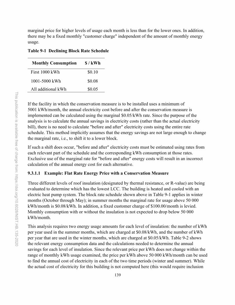
139

This p

ublica

tion is ava

ilab

le free

of ch

arge

from: h

ttps://doi.o

rg/1

0.6

028

/NIS

T.H

B.13

5-202

0

marginal price for higher levels of usage each month is less than for the lower ones. In addition, there may be a fixed monthly "customer charge" independent of the amount of monthly energy usage.

Table 9-1 Declining Block Rate Schedule

Monthly Consumption $ / kWh

First 1000 kWh $0.10

1001-5000 kWh $0.08

All additional kWh $0.05

If the facility in which the conservation measure is to be installed uses a minimum of 5001 kWh/month, the annual electricity cost before and after the conservation measure is implemented can be calculated using the marginal $0.05/kWh rate. Since the purpose of the analysis is to calculate the annual savings in electricity costs (rather than the actual electricity bill), there is no need to calculate "before and after" electricity costs using the entire rate schedule. This method implicitly assumes that the energy savings are not large enough to change the marginal rate, i.e., to shift it to a lower block.

If such a shift does occur, "before and after" electricity costs must be estimated using rates from each relevant part of the schedule and the corresponding kWh consumption at those rates. Exclusive use of the marginal rate for "before and after" energy costs will result in an incorrect calculation of the annual energy cost for each alternative.

9.3.1.1 Example: Flat Rate Energy Price with a Conservation Measure

Three different levels of roof insulation (designated by thermal resistance, or R-value) are being evaluated to determine which has the lowest LCC. The building is heated and cooled with an electric heat pump system. The block rate schedule shown above in Table 9-1 applies in winter months (October through May); in summer months the marginal rate for usage above 50 000 kWh/month is $0.08/kWh. In addition, a fixed customer charge of $100.00/month is levied. Monthly consumption with or without the insulation is not expected to drop below 50 000 kWh/month.

This analysis requires two energy usage amounts for each level of insulation: the number of kWh per year used in the summer months, which are charged at $0.08/kWh, and the number of kWh per year that are used in the winter months, which are charged at $0.05/kWh. Table 9-2 shows the relevant energy consumption data and the calculations needed to determine the annual savings for each level of insulation. Since the relevant price per kWh does not change within the range of monthly kWh usage examined, the price per kWh above 50 000 kWh/month can be used to find the annual cost of electricity in each of the two time periods (winter and summer). While the actual cost of electricity for this building is not computed here (this would require inclusion

140

This p

ublica

tion is ava

ilab

le free

of ch

arge

from: h

ttps://doi.o

rg/1

0.6

028

/NIS

T.H

B.13

5-202

0

of the customer charge and the higher kWh prices for the first 50 000 kWh/month), these additional costs would be the same for each insulation level and thus will not affect the annual savings.

Table 9-2 Annual Consumption and Cost for Roof Insulation Retrofit

Alternative

Consumption (kWh) Cost

Winter Summer Winter @ $0.05 Summer @ $0.08 Annual Cost Annual Savings

Existing 600 000 300 000 $30 000 $24 000 $54 000 -- Add R-5 570 000 285 000 $28 500 $22 800 $51 300 $2700 Add R-10 560 000 280 000 $28 000 $22 400 $50 400 $3600 Add R-15 555 000 277 000 $27 750 $22 160 $49 910 $4090

Compare the annual energy cost for a building using the consumption shown in Table 9-2 at the "existing insulation" level and subject to the rate schedule shown above with the annual energy cost for the same building heated with natural gas. Assume that the electricity usage for the gas-heated building is 5000 kWh/month in the winter months, so that total electricity usage during those months is 40 000 kWh (8 months * 5000 kWh/month). Assume that the total natural gas usage for the winter months is 1790 GJ (1700 MMBtu or 17 000 therms) billed at a flat rate of $5.20/GJ ($5.49/MMBtu), plus a monthly customer charge of $100.00. If the total energy cost for each of these two buildings is being compared, the energy costs should reflect the customer charges and the block rate structure applied to the electricity costs. The solution can be calculated as follows:

141

This p

ublica

tion is ava

ilab

le free

of ch

arge

from: h

ttps://doi.o

rg/1

0.6

028

/NIS

T.H

B.13

5-202

0

(1) All Electric Building 12 month * $100/month =$1200 + 12 months * 10 000 kWh/month * $0.10/kWh =$12 000 + 12 months * 40 000 kWh/month * $0.08/kWh =$38 400 + (300 000 kWh – 4 months * 50 000 kWh/month) =100 000 * 0.08 = $8000 + (600 000 kWh – 8 months * 50 000 kWh/month) =200 000 * $0.05 = $10 000 Total Annual Energy Cost =$69 600 (2) Gas Heated Building Electricity Cost 12 month * $100/month =$1200 + 12 months * 10 000 kWh/month * $0.10/kWh =$12 000 + 12 months * 40 000 kWh/month * $0.08/kWh =$38 400 + (300 000 kWh – 4 months * 50 000 kWh/month) =100 000 * $0.08 = $8000 Total Annual Electricity Cost =$59 600 Natural Gas Cost 12 month * $100/month =$1200 + 1790 GJ * $5.20 / GJ =$9310 Total Annual Natural Gas Cost =$10 510 Total Annual Energy Cost =$70 110

Conclusion: The annual energy cost of the all-electric building is $510 lower than the building using both electricity and natural gas, at base-date energy prices.

If only the heating costs are to be compared, the 200 000 kWh (600 000 kWh - 400 000 kWh) used for space heating at $0.05/kWh provides the annual cost of electric space heating. (The customer charge for electricity and the other kWh consumption costs will still be incurred if the heating system is switched to natural gas.) Compare this with the total annual natural gas cost, including both the monthly customer charge and energy charge for 179 GJ/year. The customer charge for natural gas must be included in this cost since this would be avoided entirely in the all-electric building.

(1) Electric Heating Only 200 000 kWh * $0.05/kWh = $10 000 (2) Gas Heating Only 12 months * $100/month customer charge = $1200 + 1790 GJ * $5.20/GJ = 9310 Total Annual Natural Gas Cost = $10 510

Both solution methods show that heating with natural gas would cost $510 more annually at current prices than heating with the electric heat pump system, given the non-escalating utility rates shown.

142

This p

ublica

tion is ava

ilab

le free

of ch

arge

from: h

ttps://doi.o

rg/1

0.6

028

/NIS

T.H

B.13

5-202

0

9.3.2 Time-Varying Pricing (TVP)

Time-varying pricing, such as time-of-use (TOU) rate schedules for electricity prices exist to different extents across the United States. Typically, under a TOU schedule, different set rates are levied for usage at different times of the day and for different days of the week. For example, residential prices may be low during late night and early morning hours, moderate during mid-day hours and on weekends, and high during the peak demand hours (mid-morning and early evening) on weekdays. These rate schedules may vary by month of the year as well, especially if the utility has a pronounced summer or winter peak. Real-time and day-ahead pricing, which provide a unique price for every time period (e.g., hourly), have become prevalent across the U.S. and are now the default rates for many commercial and industrial customers; moreover, these and other such dynamic rates (i.e., ones that respond to underlying wholesale market conditions) are routinely offered by 3rd-party suppliers in numerous U.S. states that are de-regulated/restructured (i.e., where customers have electric choice) (Barbose, Goldman, & Neenan, 2004).

Calculating annual electricity costs using TVP rates, even just TOU ones, can be complicated, regardless of whether these are to be used in an LCCA. The most challenging part of TOU calculations is determining the quantity of energy consumed in each pricing period. This usually requires an hourly analysis of the energy requirements of a building system for each design alternative being considered. Energy cost calculations with TOU rates are especially critical for projects that shift usage from one period to another (e.g., energy storage systems) or involve on-site energy generation that is time-specific (e.g., solar photovoltaic power).

If a project is expected to reduce usage proportionally in each pricing period, the annual savings for that project can be calculated using the same average price for both the "before and after" cases. If the project is expected to affect usage in some periods more than others (e.g., a programmable thermostat to lower indoor temperature settings during unoccupied hours), the savings (and additional cost in the case of load shifting) must be calculated for each pricing period and summed to arrive at an annual rate.

Table 9-3 shows a TOU rate and corresponding usage in each pricing period to be used in evaluating a proposed battery storage project. This project is expected to reduce electricity usage by 50 000 kWh annually during on-peak pricing periods but increase off-peak usage by 60 000 kWh annually. The expected annual savings is $6000 ($45 000 - $39 000). Note that the same result would be obtained by multiplying the annual usage by the corresponding weighted average price. But this weighted average price must be calculated separately for both cases (the base case and alternative). A single average price for the year will not give the correct result for this example because the project does not affect all periods proportionally.

143

This p

ublica

tion is ava

ilab

le free

of ch

arge

from: h

ttps://doi.o

rg/1

0.6

028

/NIS

T.H

B.13

5-202

0

Table 9-3 Annual Costs with Time-of-Use Rates

Rate Period Base Case Alternative

Annual kWh

Annual Cost

Annual kWh

Annual Cost

Off peak hours@ $0.025/kWh 100 000 $2500 160 000 $4000 Shoulder hours@ $0.050/kWh 250 000 $12 500 250 000 $12 500 Peak hours @ $0.150/kWh 200 000 $30 000 150 000 $22 500 Total annual cost 550 000 $45 000 560 000 $39 000 Weighted average cost $0.082 $0.070

9.3.3 Demand Charges

Demand charges are energy costs that are related to peak usage, usually measured over a short time interval (e.g., 15 minutes). Peak energy use of this sort is called peak power demand, and for electricity is typically measured in kW. Demand charges are generally levied monthly. For some users (especially ones with low “load factors”), demand charges can make up as much as half of the monthly and annual electricity cost. Residential electricity rates do not typically include a demand charge, but this may become more common as “interval” meters (rather than ones that only measure cumulatively) and on-site renewable and storage are more widely adopted.

Demand charges can be relatively simple to calculate when they are levied in direct proportion to peak demand. If demand charges are levied as a flat rate per kW, the reduction in annual demand costs attributable to an energy conservation project can be calculated once the corresponding reduction in peak monthly kW demand has been determined. Simply multiply the reduction in kW demand each month times a “diversity factor” (i.e., the percentage of the load reduction that is expected to be in effect at the peak period each month, such as 80% for overhead lighting) by the monthly demand charge for that month and sum these charges for the 12 months of the year.

However, rates with demand charges are sometimes more complex. Although becoming less common, "ratchet" clauses that use peak kW demand in previous months in calculating the demand charge for the current month still may exist and will require careful analysis. In addition, demand charges can associate with TOU rates, where a higher demand charge would be levied during periods of peak utility demand (e.g., between 12 and 8 P.M.), and lower or no charge levied during off-peak periods. As with the case of kWh cost calculations, the more complex the demand charge, the more information about kW demand is required both with and without the project. This requires careful consideration when selecting and running an appropriate building energy simulation program.

9.3.4 Utility Programs and Regulation

The great majority of utilities have programs on energy efficiency, renewable energy, and/or demand response (load shedding and shifting).

144

This p

ublica

tion is ava

ilab

le free

of ch

arge

from: h

ttps://doi.o

rg/1

0.6

028

/NIS

T.H

B.13

5-202

0

Demand response programs can provide facilities the opportunity to significantly reduce energy costs in exchange for quickly shedding load to reduce stress on the electricity grid at the request of the utility.

Depending on the state, the regulations on selling excess electricity (e.g., from renewable energy or cogeneration installations) back to the utility vary significantly. Most states provide net metering but allow for different levels of compensation for excess electricity production.

9.4 Whole Building LCCA

The discussion thus far has primarily focused on LCCA of individual systems that have mostly been assumed independent of other building aspects. However, many projects will impact multiple systems and/or include multiple system options, such as those discussed in Section 7.4, where facility components interact and changing one aspect of the facility impacts performance of other components and the entire facility. Facility performance includes multiple criteria, including facility functional requirements, energy and water consumption, and occupant productivity, comfort, and health. Each of these criteria should be considered for inclusion in the LCCA through available metrics, whether with monetary or non-monetary values, as discussed in Section 4.7.

For example, decreasing the air leakage through a building envelope can reduce the loads on the HVAC system (lowering energy consumption), improve occupant thermal comfort (reducing drafts), and decrease stress on the local electricity grid (lowering peak demands). At the same time, the lower air leakage rates may lead to less ventilation of occupied spaces, causing higher levels of VOCs that could lead to occupant health issues. This example emphasizes the need to take an integrated system approach to facility design. Evaluating the cost-effectiveness of facility and building construction and renovation (e.g., deep energy retrofits) requires the completion of a whole-building LCCA that analyzes the implications across the entire building.

Evaluating whole buildings will typically require a longer study period (30 or 40 years) because many building decisions will be in place for decades (e.g., building envelope, HVAC ductwork, and renewable energy systems) and the facility itself will likely remain in place for 50 years or longer. Additionally, whole building simulation will be needed to accurately estimate the net effect of changing multiple systems within the building design on the building’s energy and water consumption, air flow and contaminant levels, and occupant comfort.

These same considerations should be applied to projects executed as part of a facility- or campus-level master plan, whether the goal is focused on energy, water, or a combination of these and other performance targets. Each project should be viewed through the lens of the master plan to ensure that the combination of projects to be implemented will minimize LCC across the entire facility or campus. Taking this view can become complicated because a set of projects included in a master plan may have different initial investment costs, OM&R costs, and residual values, as well as different levels of resilience and service lives.

145

This p

ublica

tion is ava

ilab

le free

of ch

arge

from: h

ttps://doi.o

rg/1

0.6

028

/NIS

T.H

B.13

5-202

0

Due to the nearly infinite combination of potential project designs for a building, facility, or campus, it is of great importance to narrow down the alternatives to consider in the LCCA those that are technically feasible. Each alternative should meet all functional and performance requirements for the specific project(s). These could include meeting energy efficiency or sustainability goals, mission criticality, resilience, occupant health requirements, productivity targets, or risk levels. Any alternative that does not meet those requirements should be excluded.

Similarly, these functional and performance requirements should be considered in the LCCA. If feasible, any differences across alternatives in functionality and performance should be quantified using monetary or non-monetary metrics. These metrics will be included in the LCCA report to provide the project decision maker with a holistic view of the benefits and costs of the project alternatives.

Figure 9-1 shows two examples related to resilience (i.e., ability to prepare for, withstand, and recover from disruptions caused by major accidents, attacks, or natural disasters). On the left is the choice between a base case (B.C.) and alternative (Alt. 1) for new construction that must meet a minimum level of resilience (bottom of y-axis). Alternative 1 leads to lower overall LCC while providing the same level of resilience.

On the right is a similar example for a retrofit project to meet the same level of resilience. In this case, the current building (B.L.) does not meet the resilience requirement, and is therefore not a viable alternative. Instead the decision will be made between the base case (B.C.) and alternative (Alt. 1) that both meet the resilience requirement. As in the prior example, Alternative 1 has the lowest LCC.

Figure 9-1 LCCA with a Resilience Requirement18

18 Source: A. Zhivov (2018)

146

This p

ublica

tion is ava

ilab

le free

of ch

arge

from: h

ttps://doi.o

rg/1

0.6

028

/NIS

T.H

B.13

5-202

0

Consider the prior example with another alternative (Alt. 2) that provides resilience beyond the minimum requirement, but at a slightly higher LCC than that for Alternative 1. The LCC analyst should provide the difference in resilience performance in their LCCA report to ensure the decision maker understands the trade-offs between projects (i.e., the benefit of additional resilience in exchange for some additional cost).

A quantitative example based on this example will be discussed in Chapter 13.

147

This p

ublica

tion is ava

ilab

le free

of ch

arge

from: h

ttps://doi.o

rg/1

0.6

028

/NIS

T.H

B.13

5-202

0

148

This p

ublica

tion is ava

ilab

le free

of ch

arge

from: h

ttps://doi.o

rg/1

0.6

028

/NIS

T.H

B.13

5-202

0

10 Alternative Funding Options

Thus far this handbook has focused on federally-funded projects with budget constraints (e.g., congressional appropriations). However, budget constraints may lead cost-effective projects to be foregone. Where appropriations are unavailable or insufficient, alternative options can provide the required initial investment. These investments are typically paid back over time using the avoided costs they generate. Studies indicate these options may generate even greater avoided cost than the same investment using direct federal funding. This chapter will summarize potential alternative approaches to funding projects, with focus on energy savings performance contracts (ESPCs), and provide examples of how to evaluate these options using methodology consistent with LCCA.

10.1 Background

As was discussed in the Preface, the National Energy Conservation Policy Act (NECPA) is the primary statutory authority directing federal agencies to improve energy management in their facilities and operations. First authorized by Congress in 1986 as an alternative financing method to traditional Federal procurement requirements, ESPCs allow Federal agencies to engage with private sector energy service companies to implement energy conservation measures and water conservation measures that reduce the Federal government’s energy and operating costs, while creating private sector jobs and improving Federal infrastructure. Section 155(a) of the Energy Policy Act of 1992 (Pub. L. No. 102-486) directed DOE, with the concurrence of the Federal Acquisition Regulatory Council, to “establish procedures and methods for use by Federal agencies to select, monitor, and terminate contracts with energy service contractors.

Moreover, in implementing Executive Order 13834: Efficient Federal Operations (May 2018), which directs federal agencies to manage buildings, vehicles, and operations to optimize energy and environmental performance, reduce waste, and cut costs, CEQ explicitly states that performance contracting should be utilized to “achieve energy, water, building modernization, and infrastructure goals” when “life-cycle cost-effective to maximize efficiency and economic benefits” (CEQ, 2019b).

Accordingly, to meet the requirements of federal energy management statutes, federal agencies can access multiple sources of funding for capital investments (FEMP, 2011b, 2019e):

(1) direct appropriations (2) energy savings performance contract (ESPC) (3) utility energy service contract (UESC) (4) energy incentive programs (5) other private investment options (e.g., power purchase agreement (PPA), enhanced use

leases)

The use of alternative funding options for federal investment in efficiency improvements in proportion to the use of appropriated funds has risen over time. From 2005 to 2017, federal

149

This p

ublica

tion is ava

ilab

le free

of ch

arge

from: h

ttps://doi.o

rg/1

0.6

028

/NIS

T.H

B.13

5-202

0

investment in facility efficiency improvements totaled over $23 billion across approximately 2800 projects (CRS, 2018; DOE, 2019a; FEMP, 2019a). Figure 10-1 shows federal investment (adjusted for inflation) in facility efficiency improvements for 2010 through 2018 (CEQ, 2019a). Prior to 2016, annual direct obligations accounted for most of the investment funding. Since 2016, ESPC has been the primary funding mechanism for federal efficiency investments. UESCs have smaller relative investments, fluctuating between $74 million and $216 million annually.

Figure 10-1 Federal Investment in Facility Efficiency Improvements19

This chapter provides an overview of these alternative financing options. The most common to date are ESPCs and UESCs, but other options (e.g., energy incentive programs, PPAs, enhanced use leasing) focused primarily on funding distributed energy activities are expected to increase in the future.

19 CEQ (2019a)

150

This p

ublica

tion is ava

ilab

le free

of ch

arge

from: h

ttps://doi.o

rg/1

0.6

028

/NIS

T.H

B.13

5-202

0

10.2 ESPC

Energy savings performance contracts (ESPCs) are contracts between a Federal agency and an energy service company (ESCO) that allow Federal agencies to procure facility improvements that are paid for through energy savings, with no required up-front capital costs or appropriations from Congress. ESPCs present an opportunity for Federal agencies to reduce energy costs through a collaborative effort to identify affordable energy solutions that promote energy reliability, affordability, and security. An ESPC is a collaborative effort between a federal agency and an energy service company (ESCO). Multiple executive orders, most recently EO 13834, recommend this method of financing for resource conservation projects. After being selected for a potential award, the ESCO conducts a comprehensive facility audit and identifies improvements to save energy and water and reduce utility and related operation and maintenance costs. In consultation with the agency, the ESCO designs and constructs a project that meets the agency's needs, arranges financing to pay for the project, and guarantees the savings (FEMP, 2011b).

10.2.1 Background

While an agency may contribute funds to an ESPC project, an ESCO incurs all costs of implementing energy and water savings measures, including performing the audit, designing the project, acquiring and installing the equipment, and training personnel. While operating and maintaining equipment can be assigned to either the agency or ESCO, by law the ESCO is ultimately responsible to assure proper maintenance and repairs are conducted to sustain the savings guarantee. The ESCO receives agency payments not to exceed the energy cost savings and/or energy-related cost savings (defined by 10 CFR 436 Subpart B to include related O&M savings, as well as water savings)20 directly resulting from implementation of energy conservation measures each year for the term of the contract (which may not exceed 25 years). This payment is the sum of all elements due to the ESCO in a contract year. Included are the debt service, along with contractor payments for O&M, measurement and verification (M&V), and any other service included in the contract.

10.2.1.1 ESPC Rules and Requirements

To reduce the risk of shortfalls and the resulting decreased payments, ESCOs typically guarantee less than their estimated cost savings. These guaranteed savings are used to determine annual contract payments. Guaranteed savings may include avoided costs related to O&M and R&R, as well as revenues the projects may enable from sources such as demand response programs or the sale of renewable energy credits (RECs) generated by the project.21 Additional savings not

20 For more discussion of what is included in energy cost savings and energy-related cost savings, see FEMP's “Practical Guide to Savings and Payments in FEMP ESPC Task Orders Rev. 3” (FEMP, 2009). 21 A recent study estimated the average guaranteed savings in ESPCs to be approximately 92 % of those estimated (Slattery, 2018). Reported cost savings vary over time but on average represent a combination of energy and water cost savings (averaging roughly 75 %) and operations, maintenance, repair and replacement (OMR&R) savings (averaging roughly 25 %) (Slattery, 2018).

151

This p

ublica

tion is ava

ilab

le free

of ch

arge

from: h

ttps://doi.o

rg/1

0.6

028

/NIS

T.H

B.13

5-202

0

necessary to make a project economic need not be included in the contract if these savings are difficult to evaluate and include in a firm fixed-price contract. Examples are certain O&M savings and funds from utility demand response programs, which are often unpredictable and variable.

Agencies can apply appropriated funds that would have been spent on energy or water conservation measures to the ESPC, including costs of planned new equipment and repair or replacement of failing or failed equipment (FEMP, 2009). Appropriated funding for installations required to meet renewable energy, sustainability, and/or resilience requirements (e.g., solar photovoltaic plus battery storage to ensure continuity of operations) can also be applied to the ESPC. The first example in Section 10.2.3 includes agency funds allocated to the ESPC for replacement of failing equipment that would otherwise have been expended by the agency without an ESPC.

Specific rules on ESPCs include the following:

General ESPC Rules:

• Must save energy, water, or wastewater • Cost savings may come from reduced utility, O&M, and/or repair and replacement (R&R)

costs • ESPCs can include a combination of energy efficiency, water conservation, and renewable

energy measures (conservation measures) • ESPCs can bundle long- and short-payback conservation measures to achieve life-cycle cost-

effectiveness • An ESPC can include multiple facilities across geographical regions within an agency in a

single contract, task or delivery order. • Agencies may enter into contracts for up to 25 years

Agency Requirements:

• Funds must be available to cover ESPC payments in the first fiscal year of the contract, task or delivery order award.

• An agency may contribute funds

ESCO Requirements:

• ESCOs incur all costs of implementing the conservation measures • ESCOs guarantee savings to agencies over the length of the contract • Annual guaranteed savings must exceed the contract payments in each year of the contract • Annual measurement and verification (M&V) reports must be submitted by the ESCO to verify

whether the guaranteed savings have been achieved. • After the contract ends, all cost savings accrue to the agency

152

This p

ublica

tion is ava

ilab

le free

of ch

arge

from: h

ttps://doi.o

rg/1

0.6

028

/NIS

T.H

B.13

5-202

0

Importantly, under the statute and the ESPC regulations, the project must be life-cycle cost-effective under 10 CFR 436, Subpart A. Life-cycle cost-effectiveness may be determined in accordance with Part 436, Subpart A using an approach that views ECMs in the context of all contemplated ECMs (i.e., the “bundle” of ECMs) under the same ESPC. 22 Notably, the ESPC statute requires the agency to realize net savings each year of the ESPC contract term. Therefore, ECMs completed using an ESPC will be life-cycle cost-effective at the end of the ESPC contract term. For example, as described more below, using the net-savings methodology in 10 CFR 436, Subpart A, a project’s ECMs must have a positive net savings over the term of the LCCA study period (as determined in 10 CFR 436.14(d)-(e)) in order to be life-cycle cost-effective. ECMs completed using an ESPC, which has net savings each year of the contract, will be life-cycle cost-effective if the LCCA study period is the length of the ESPC contract term. However, even though ESPC projects are inherently life-cycle cost-effective over the course of the contract term, pursuant to 42 U.S.C. 8254, agencies must still perform LCCA for ESPC projects by using the methodologies contained in 10 CFR 436, Subpart A, and this handbook. Importantly, the study period for a project’s ECMs, as established in 10 CFR 436.14(d)-(e), may not end with the termination of the ESPC contract term, so agencies must ensure that LCCA for ECMs completed using ESPC financing include any applicable time periods outside of the ESPC contract term (not to exceed 40 years). As discussed in Section 2.4, a project’s study period can be either it’s the useful life of its expected longest-lasting ECM or 40 years, whichever is shorter. For the purposes of ESPC, if the project is expected to generate a positive cash flow in the period following the conclusion of the contract up to the 40-year maximum study period, the LCCA requirement should be satisfied.

10.2.1.2 Renewable Energy and Distributed Generation

Renewable energy and other “distributed generation” (e.g., combined heat and power or cogeneration) projects can be included in an ESPC. For on-site electricity generation measures that do not reduce facility consumption, per se, a source (as opposed to site) energy analysis can be used to show energy savings (OMB M-12-21, 2012). Renewable energy generation can be accomplished through an ECM where the agency owns the equipment (such as a solar photovoltaic system), or an ECM where the private developer maintains ownership until late in the contract term (OMB M-12-21, 2012). Purchase of electricity from a renewable source can be an ECM in an ESPC called an energy sales agreement (ESA), which is structured like a PPA.

Since the generating asset in an ESA is owned by the private entity, tax incentives, solar renewable energy credits (SRECs), and modified accelerated cost recovery system (MACRS) depreciation (over five years) are available and may result in lower electricity rates, making a project possible that might otherwise be noneconomic (IRS, 2017). To meet the IRS interpretation of the investment tax credit rules, the ESA component of an ESPC cannot exceed 20 years and must meet all the rules that govern ESPC implementation. At the end of the

22 For more information on “bundling,” see FEMP’s DOE Guidance on the Statutory Definition of Energy/Water Conservation Measures (ECMs) and Determining Life-Cycle Cost-Effectiveness for ESPCs with Multiple or Single ECMs (August 2013).

153

This p

ublica

tion is ava

ilab

le free

of ch

arge

from: h

ttps://doi.o

rg/1

0.6

028

/NIS

T.H

B.13

5-202

0

contract, the agency must purchase the renewable energy generation asset at its fair market value as determined by an independent appraiser at the time of sale (IRS, 2017). The ESPC ESA can be designed to include a “reserve fund,” paid for through the regular payments to the ESCO, that can be used for the asset’s purchase at the end of the contract.

10.2.1.3 ESPC Contracting Vehicles and Results

FEMP's “Practical Guide to Savings and Payments in FEMP ESPC Task Orders Rev. 3” (FEMP, 2009), the documents cited below in this sub-section, and other applicable FEMP documents should be consulted before attempting to award or evaluate an ESPC. Most federal ESPC projects have been implemented as task orders awarded under DOE indefinite-delivery, indefinite-quantity (IDIQ) ESPCs. The DOE ESPC IDIQs were established to streamline the ESPC process and make ESPC procurements practical and cost-effective for agencies. DOE awarded these overarching IDIQ (or "umbrella") ESPCs to competing ESCOs that were best qualified to serve federal agencies under the terms and conditions in the DOE IDIQ ESPCs. Note that price reasonableness of an IDIQ quote is still required and must comply with Federal Acquisition Regulation (FAR) 15.404-1 (Shonder & Atkin, 2005). Others have been awarded through the Army Corps of Engineers Multiple Award Task Order Contract (MATOC), which is similarly structured to DOE’s IDIQs.

It is difficult to cost-effectively complete small projects following the procedures in the standard DOE ESPC IDIQs. Therefore, DOE launched an alternative process, ESPC ENABLE, to streamline ESPCs specifically for small sites (particularly suitable for projects up to 18 581 m2 (200 000 ft2), though there is no size limit and many larger projects have been implemented) that need standard or targeted conservation measures. ENABLE ESPCs offer tools and templates that can allow agencies to award a task order significantly faster than large, more complex projects. These ESPCs are procured through the GSA Federal Supply Schedule SIN 334512 (FEMP, 2019b).

According to FEMP, over 400 projects have been awarded under ESPC IDIQs since 1998 with more than $6 billion of investment in energy efficiency, water conservation, and renewable energy improvements to federal facilities. These investments are projected to save $13.9 billion in cumulative utility and O&M cost savings. The magnitude of total investment through ESPCs has grown over recent years, with FY2018 DOE ESPC IDIQ-awarded task orders for $809 million (FEMP, 2019a).

The U.S. Army Corps of Engineers has an IDIQ MATOC led by U.S. Army Corps of Engineers (USACE) Engineering and Support Center, Huntsville covering government installations or facilities throughout the U.S., Republic of the Marshall Islands, U.S. Territories and Possessions, Germany, and South Korea. Between 2009 and 2017, MATOC ESPC projects have led to annual savings of $108 million as well as reductions of 3 billion gal of water and 4 million MMBtu of energy (10 % reduction) (USACE, 2018).

154

This p

ublica

tion is ava

ilab

le free

of ch

arge

from: h

ttps://doi.o

rg/1

0.6

028

/NIS

T.H

B.13

5-202

0

There still exists a perception that agency bid-to-specification projects can accomplish the same utility savings at lower costs than ESPCs, particularly if there is in-house expertise to complete the projects. However, Coleman, Earni, and Williams (2014) found that federal ESPC projects reported substantially higher savings realization rates than non-ESPC federal projects for both energy (102% versus 67%. respectively) and water conservation (122% versus 87%, respectively), though the measurement and verification (M&V) actors and methodologies for the two types differed (ESCOs and agencies perform the M&V using FEMPs M&V guidelines for the ESPCs, while federal employees or contractors perform the M&V for the non-ESPCs using methods that are not standardized). Slattery (2018) found that of 172 ESPC projects with M&V reports, verified savings were 108% of the ESCO-guaranteed savings and 99% of the estimated savings.

These results provide support that projected and verified performance of federal ESPCs align well, which leads to minimal risk to an agency, and the savings exceed that of using agency funds through standard procurement. Therefore, FEMP has recommended that the only case in which agency would use its own funds for a standard procurement of an efficiency project would be if the agency has the necessary funding needed and no other unmet capital needs for which to use the funding. Otherwise, if an ESPC project is viable (i.e., with net savings > 0), it should be completed through an ESPC.

10.2.2 Economic Analysis for ESPCs

Although ESPCs have their own unique set of requirements, these are consistent with the cost-effectiveness requirements defined in this handbook as specified in 10 CFR 436 Subpart A. While 10 CFR 436.18 specifies several methods by which cost-effectiveness may be measured, one of these measures, net savings, provides an intuitive means of determining the cost-effectiveness of ESPCs. As described in Section 6.1 (consistent with 10 CFR 436 Subpart A), the net savings are calculated by taking the discounted present value of the cost savings over the study period, which could be the length of the contract or longer (up to 40 years). Using net savings, LCCA of a typical ESPC is relatively simple because there is no initial investment on the part of the agency. Therefore, per federal ESPC requirements, the annual energy savings are greater than the annual contract payments each year and all obligations are met within 25 years. If cash flow is expected to be positive for any remainder of the study period beyond the contract term, then the ESPC is cost-effective (i.e., net savings > 0).

As discussed in Section 2.2 and Section 2.3, the defined scope and objectives, as well as the constraints on the project, will impact the LCCA. For example, many ESPCs are focused on reducing energy consumption relative to a “business-as-usual” baseline. In this case the cost savings are estimated relative to expected consumption in the future. However, an ESPC could also be used to meet an agency goal, such as meeting minimum renewable energy consumption targets that require renewable generating capacity installation, regardless of the financing mechanism selected. In this case the baseline for the LCCA is the agency installing on-site renewable capacity using direct funding. Agency funds that would have been spent on this

155

This p

ublica

tion is ava

ilab

le free

of ch

arge

from: h

ttps://doi.o

rg/1

0.6

028

/NIS

T.H

B.13

5-202

0

installation can be used towards an ESPC because they are avoided costs that would have otherwise been spent to meet the agency goal. A similar example is a need to meet some greenhouse gas or resilience metric (e.g., continuity of operations during a one- or two-week grid outage) that would require new equipment installation. Any agency funds required to meet the resilience goal through directly funding the project could be allocated to an ESPC.

Annual energy cost savings should include both energy consumption savings and power demand savings (if applicable), based on current local utility rates. Typically, all project guaranteed savings are dedicated to making contract payments. Using less will either lengthen the contract term, incurring more debt service costs, or lead to lower project investment.

Less than ideal O&M schedules (e.g., deferred maintenance) will lead to more repairs and shorter equipment lifetimes, resulting in higher future costs for agencies. However, avoided O&M cost estimates must use forecasted budgeting and spending patterns instead of ideal spending levels to maintain optimal performance. Therefore, the considered project may lead to greater avoided repair and replacement costs than what is reflected in the project’s financial schedules (FEMP, 2009). An example of deferred maintenance evaluation can be found in Chapter 14.

10.2.3 ESPC Economic Analysis Examples

As has been discussed, an ESPC is an alternative to agencies directly funding needed or beneficial projects to meet an agency goal. This section provides two examples of ESPC economic analysis that is consistent with the LCC methodology in this handbook and 10 CFR 436, Subpart A. In both examples, the ESCO covers the costs for all project activities and the agency makes payments to the ESCO from funds that could have otherwise been spent on energy and energy-related expenses, as well as expenses related to equipment replacements. However, the appropriate baseline case for each example is different, the first assuming the agency continues with business-as-usual activities and the second assuming the agency must complete a project to meet an agency goal.

The first example is focused on reducing operational costs by improving a building’s energy efficiency. Assume the ESPC implements multiple ECMs:

Boiler plant improvements

Building automation systems / energy management controls systems

Lighting improvements

Building envelope modifications

Renewable energy systems

Water and sewer conservation systems

The boiler plant improvements include replacement of two boilers, one that has reached the end of its rated useful life (and is continuously breaking down) and another that is expected to start failing within the next five years. Therefore, the replacement costs for the boilers ($350 000 for

156

This p

ublica

tion is ava

ilab

le free

of ch

arge

from: h

ttps://doi.o

rg/1

0.6

028

/NIS

T.H

B.13

5-202

0

each) would occur regardless of whether the ESPC is implemented and, therefore, represent avoided costs for the agency in Year 1 and Year 5. The agency allocates those funds toward payments to the ESCO (to be made after the ESCO’s investments in the equipment and installation in those two years).

Table 10-1 shows the cash flows and savings to the agency over a 25-year study period relative to a business-as-usual scenario. The ESPC leads to guaranteed net savings (NS) every year of the contract. The present value of net guaranteed savings over the study period is $463 000. The present value of net estimated savings is even higher at $2.46 million. This is because the ESPC only guarantees 96 % of the projected savings and the contract payments end in year 23, leaving two years of cost savings with no contract payments at the end of the study period. The ESPC is LCC-effective because there are positive NS as compared to using the non-ESPC, business-as-usual alternative (i.e., continued O&M and R&R of the current boiler and other building energy systems) over the 25-year study period. Additionally, the more restrictive requirement on ESPCs of realizing (guaranteed) savings every year of the contract is also met.

For other examples of ESPC evaluation, see Chapter 11.

157

This p

ublica

tion is ava

ilab

le free

of ch

arge

from: h

ttps://doi.o

rg/1

0.6

028

/NIS

T.H

B.13

5-202

0

Table 10-1 Example ESPC Cash Flow

Year Estimated Cost Savings

Gtd. Cost Savings

Payments Gtd.

Nominal Savings

Gtd. PV NS

Est. Nominal Savings

Est. PV NS

0 $0 $0 $0 $0 $0 $0 $0

1 $1 067 775 $1 039 064 $925 434 $113 630 $110 321 $142 341 $138 195

2 $738 657 $709 110 $692 701 $16 409 $15 467 $45 956 $43 318

3 $760 146 $729 740 $712 854 $16 886 $15 453 $47 292 $43 279

4 $782 261 $750 971 $733 593 $17 378 $15 440 $48 668 $43 241

5 $1 155 020 $1 122 819 $1 104 936 $17 883 $15 426 $50 084 $43 203

6 $828 441 $795 303 $776 900 $18 403 $15 413 $51 541 $43 165

7 $852 544 $818 442 $799 503 $18 939 $15 399 $53 041 $43 127

8 $877 348 $842 254 $822 764 $19 490 $15 386 $54 584 $43 089

9 $902 875 $866 760 $846 703 $20 057 $15 372 $56 172 $43 051

10 $929 144 $891 978 $871 338 $20 640 $15 358 $57 806 $43 013

11 $956 178 $917 931 $896 690 $21 241 $15 345 $59 488 $42 975

12 $983 999 $944 639 $922 780 $21 859 $15 331 $61 219 $42 938

13 $1 012 630 $972 125 $949 630 $22 495 $15 318 $63 000 $42 900

14 $1 042 094 $1 000 410 $977 261 $23 149 $15 305 $64 833 $42 863

15 $1 072 416 $1 029 519 $1 005 696 $23 823 $15 291 $66 720 $42 825

16 $1 103 620 $1 059 475 $1 034 959 $24 516 $15 278 $68 661 $42 787

17 $1 135 733 $1 090 304 $1 065 074 $25 230 $15 264 $70 659 $42 750

18 $1 168 781 $1 122 030 $1 096 066 $25 964 $15 251 $72 715 $42 712

19 $1 202 790 $1 154 678 $1 127 959 $26 719 $15 238 $74 831 $42 675

20 $1 237 790 $1 188 278 $1 160 781 $27 497 $15 224 $77 009 $42 638

21 $1 273 809 $1 222 857 $1 194 560 $28 297 $15 211 $79 249 $42 600

22 $1 310 876 $1 258 441 $1 229 321 $29 120 $15 198 $81 555 $42 563

23 $1 349 023 $1 295 062 $1 233 966 $61 096 $30 957 $115 057 $58 298

24 $1 388 279 $0 $0 $0 $0 $1 388 279 $682 941

25 $1 428 676 $0 $0 $0 $0 $1 428 676 $682 344

$26 560 905 $22 822 190 $22 181 468 $640 722 $463 245 $4 379 437 $2 463 491

Discount Rate = 3 %; 23 Year ESPC Contract; 25 Year Study Period

The next two scenarios assume the agency has decided to install new solar photovoltaic capacity to increase its electricity consumption to meet an alternative energy goal. An ESPC is being considered to finance the 2.5 MW on-site solar photovoltaic system installation as an alternative to the agency directly funding the project. In this case, the baseline case is the agency directly funding the installation. Any funds that would have been required to pay for this installation are

158

This p

ublica

tion is ava

ilab

le free

of ch

arge

from: h

ttps://doi.o

rg/1

0.6

028

/NIS

T.H

B.13

5-202

0

considered avoided costs in an ESPC scenario because the system was going to be installed to meet the agency’s determined need with or without an ESPC.

Assume the following for the direct-funded scenario:

Installation cost to the agency: $5 million Project is constructed in Year 0 and goes into service in Year 1 Annual maintenance costs for the system: $10 000 Annual production (Year 1): 2.5 million kWh Annual degradation rate of system: 0.5% Electric utility rate: 10 cents/kWh Study period and system service life: 25 years Real discount rate: 3 %

Based on these assumptions, the agency realizes the cash flows shown in Table 10-2. The large upfront investment costs have a simple payback of 23 years. Once the cash flows are discounted to present value, the project leads to negative net savings of over $1 million. However, since the agency has determined it necessary to install the system, the project would still be completed unless there is an alternative financing approach, such as an ESPC, that leads to lower costs to the agency.

159

This p

ublica

tion is ava

ilab

le free

of ch

arge

from: h

ttps://doi.o

rg/1

0.6

028

/NIS

T.H

B.13

5-202

0

Table 10-2 Direct-Funded Solar Photovoltaic Project Cash Flow and Net Savings

Year Installation and

Maintenance Costs ($) Gen.(kWh)

Utility Rate

($/kWh)

Nominal Net Savings ($)

PV Net Savings ($)

0 $5 000 000 - - -$5 000 000 -$5 000 000

1 $10 000 2 500 000 $0.10 $240 000 $233 010

2 $10 000 2 487 500 $0.10 $238 750 $225 045

3 $10 000 2 475 000 $0.10 $237 500 $217 346

4 $10 000 2 462 500 $0.10 $236 250 $209 905

5 $10 000 2 450 000 $0.10 $235 000 $202 713

6 $10 000 2 437 500 $0.10 $233 750 $195 762

7 $10 000 2 425 000 $0.10 $232 500 $189 044

8 $10 000 2 412 500 $0.10 $231 250 $182 551

9 $10 000 2 400 000 $0.10 $230 000 $176 276

10 $10 000 2 387 500 $0.10 $228 750 $170 211

11 $10 000 2 375 000 $0.10 $227 500 $164 351

12 $10 000 2 362 500 $0.10 $226 250 $158 687

13 $10 000 2 350 000 $0.10 $225 000 $153 214

14 $10 000 2 337 500 $0.10 $223 750 $147 925

15 $10 000 2 325 000 $0.10 $222 500 $142 814

16 $10 000 2 312 500 $0.10 $221 250 $137 876

17 $10 000 2 300 000 $0.10 $220 000 $133 104

18 $10 000 2 287 500 $0.10 $218 750 $128 493

19 $10 000 2 275 000 $0.10 $217 500 $124 037

20 $10 000 2 262 500 $0.10 $216 250 $119 732

21 $10 000 2 250 000 $0.10 $215 000 $115 573

22 $10 000 2 237 500 $0.10 $213 750 $111 555

23 $10 000 2 225 000 $0.10 $212 500 $107 672

24 $10 000 2 212 500 $0.10 $211 250 $103 921

25 $10 000 2 200 000 $0.10 $210 000 $100 297

Total PV Net Savings -$1 048 887

Alternatively, an agency could pursue an ESPC that finances the same solar photovoltaic project. For simplicity, assume that the guaranteed production is 100 % of the estimated production.23 In

23 This assumption allows for a direct comparison of the results in the two funding approaches. Typically, the guaranteed net savings in an ESPC would be less than 100 % (typically 90 % to 95 %) to ensure the guarantee can be met by the ESCO. In those cases, the guaranteed net savings will be smaller than the estimated net savings. When comparing direct funding to ESPC funding alternatives, it is appropriate to compare estimated net savings for each

160

This p

ublica

tion is ava

ilab

le free

of ch

arge

from: h

ttps://doi.o

rg/1

0.6

028

/NIS

T.H

B.13

5-202

0

this case, the installation and maintenance costs the agency would have paid are now avoided costs and treated, respectively, as non-recurring savings for the avoided installation costs and recurring savings for the avoided maintenance costs (FEMP, 2019d). The agency can choose to use some of those funds towards the ESPC project. In this example (shown in Table 10-3), $3.7 million of the $5 million in avoided installation cost (relative to the direct-funded scenario) is used for a payment in Year 1 to assist with the ESPC’s initial construction and $10 000 (representing the avoided recurring maintenance costs) in each subsequent year of the term to defray ESPC maintenance costs. The project is designed to provide $1 in nominal guaranteed savings each year. The only exception is Year 1, which accounts for almost all the project’s total avoided costs of over $5.2 million. As a result, net guaranteed savings in Year 1 are $1.26 million while the net guaranteed savings over the remainder of the contract are only $17. In this example, the net guaranteed savings are equal to the estimated net savings to be used in comparison to the prior direct funding alternative.

Note that this ESPC scenario provides 74 % of the avoided costs associated with the installation through the payment in Year 1. The agency could have chosen to provide more (or less) funding associated with those avoided costs. Actual ESPC structures will vary from project to project based on the specific scenario facing an agency.

In looking at the two scenarios together, the ESPC is more life-cycle cost-effective, as it provides a present value net savings of over $1.2 million estimated savings relative to the direct-funded option.

alternative. However, if guaranteed net savings from an ESPC is greater than estimated net savings from direct funding alternative, then that is sufficient to show the ESPC is the more cost-effective alternative.

161

This p

ublica

tion is ava

ilab

le free

of ch

arge

from: h

ttps://doi.o

rg/1

0.6

028

/NIS

T.H

B.13

5-202

0

Table 10-3 Solar Photovoltaic Project Cash Flow and Net Savings with ESPC

Year Contract Costs ($)

Gtd. Elect. Cost Savings ($)

Avoided Costs ($)

Nominal Gtd. Net

Savings ($)

PV Gtd. Net Savings ($)

0 $0 - $0 $0 $0

1 $3 959 999 250 000 $5 010 000 $1 300 001 $1 262 137

2 $258 749 248 750 $10 000 $1 $0.94

3 $257 499 247 500 $10 000 $1 $0.92

4 $256 249 246 250 $10 000 $1 $0.89

5 $254 999 245 000 $10 000 $1 $0.86

6 $253 749 243 750 $10 000 $1 $0.84

7 $252 499 242 500 $10 000 $1 $0.81

8 $251 249 241 250 $10 000 $1 $0.79

9 $249 999 240 000 $10 000 $1 $0.77

10 $248 749 238 750 $10 000 $1 $0.74

11 $247 499 237 500 $10 000 $1 $0.72

12 $246 249 236 250 $10 000 $1 $0.70

13 $244 999 235 000 $10 000 $1 $0.68

14 $243 749 233 750 $10 000 $1 $0.66

15 $242 499 232 500 $10 000 $1 $0.64

16 $241 249 231 250 $10 000 $1 $0.62

17 $239 999 230 000 $10 000 $1 $0.61

18 $238 749 228 750 $10 000 $1 $0.59

19 $237 499 227 500 $10 000 $1 $0.57

20 $236 249 226 250 $10 000 $1 $0.55

21 $234 999 225 000 $10 000 $1 $0.54

22 $233 749 223 750 $10 000 $1 $0.52

23 $232 499 222 500 $10 000 $1 $0.51

24 $231 249 221 250 $10 000 $1 $0.49

25 $229 999 220 000 $10 000 $1 $0.48

Total PV Gtd. Net Savings Relative to Agency Funded = $1 262 153

Note: Guaranteed electricity cost savings are assumed to be 100 % of the estimated savings.

162

This p

ublica

tion is ava

ilab

le free

of ch

arge

from: h

ttps://doi.o

rg/1

0.6

028

/NIS

T.H

B.13

5-202

0

10.3 UESC

Authorized by the Energy Policy Act of 1992, P.L. 102-486 (codified as 42 U.S.C. 8256), a utility energy service contract (UESC) is a limited-source contract between a federal agency and serving utility for energy management services, including energy and water efficiency improvements and demand-reduction services. UESCs help utilities improve customer load profiles, meet efficiency and renewable energy portfolio standards, and provide exemplary customer service. Federal sites benefit from UESCs by meeting federal mandates, resolving specific challenges at the site such as replacing aging equipment with new, more energy-efficient equipment, and reducing operating costs. UESCs provide a streamlined approach for federal agencies to contract for the broad spectrum of energy management services offered by their local serving utilities. To further simplify the process, FEMP’s UESC Guide serves as an important resource for federal agencies pursuing a UESC, and includes examples of and templates for UESC documents (FEMP, 2020). In a UESC, the utility partner assesses the opportunities, designs and implements the accepted energy conservation measures, and provides financing for the project, if needed. The agency then repays the utility from appropriations either at acceptance or, more commonly, over time (when the projects are financed). A UESC is appropriate for any size project—from small, single ECM projects to comprehensive, complex projects.

UESCs can be used for a wide array of energy efficiency improvements. GSA has established criteria for energy conservation measures installed in UESCs. The measure must: (1) produce measurable energy or water reductions or demand reduction; (2) be directly related to the use of energy or water, or demand reduction; and (3) the preponderance of the work (measured in dollars) must be for items (1) or (2) as well as be a direct or indirect improvement to real property. Energy management services include assessing project potential, designing solutions, providing project financing, installing the measures, and providing performance assurance. UESCs may include distributed energy.

Implementing projects through the UESC contract vehicle continues to be a major force behind many federal facilities meeting their energy management goals. Through 2020, federal agencies have employed UESCs to invest nearly $4 billion in their facilities. The FEMP Utility Program facilitates utility partnerships and utility energy services offered by serving utility companies, including electric, gas, and water. The Utility Program also encourages local utility companies to assist agencies in meeting energy efficiency, renewable energy, and water conservation goals (FEMP, 2017a). FEMP CTS shows 2100 UESC projects. Annual investment levels have consistently been between $100 million and $200 million (CRS, 2018).

As with all prospective federal energy conservation projects, LCCA for UESCs must meet the requirements of 10 CFR Subpart A. Accordingly, the methods listed in 10 CFR 436.18 (including net savings) may be used to determine life-cycle cost-effectiveness for UESCs. Unlike ESPCs, however, UESCs are not required to be paid from savings.

An economic evaluation of a UESC based on an example from the UESC Guide (FEMP, 2020) is shown in Table 10-4. Assume a government agency wants to implement a UESC with the

163

This p

ublica

tion is ava

ilab

le free

of ch

arge

from: h

ttps://doi.o

rg/1

0.6

028

/NIS

T.H

B.13

5-202

0

local utility to achieve resource conservation at a facility with an ECM bundle including HVAC, controls, lighting, and water conservation measures. The utility is tasked with evaluating, and if deemed cost-effective pursuant to 10 CFR 436 Subpart A, completing the project. Bids from subcontractors for each group of ECMs are received and evaluated based on best value (cost and quality). Five lenders provide financing quotes, and the financing option with the lowest interest rate is selected (15 years at a finance rate of 4.61 %). The utility has provided detailed energy calculations to support the projected energy savings estimates. The results find that the UESC will lead to NS of $53 670 so should be executed.

Table 10-4 UESC Example

Cost Category Cost Mechanical Equipment $2 000 000 Electrical Equipment $250 000 Lighting Equipment $950 000 Water Conservation Equipment $31 000 Total Equipment (Subcontractor) Costs $3 231 000 Contractor Labor (GSA Schedule) $3 692 077 Total Contractor Costs $6 300 000 Contractor Mark-Up 30 % $2 076 923 Total Construction Cost $9 000 000 Project Design & Development 4.63 % $416 700 Total Construction & Fees Costs $9 416 700 Utility Mark-Up 3.0 % $282 501 Project Total Cost $9 699 201 Monthly Payments pm 15-Year Loan 4.61 % $74 745 Total Present Value Financed Cost $10 146 330 Projected Present Value Savings 10 200 000 Net Savings $53 670

10.4 Other Options

Although ESPCs and UESCs are by far the most common financing mechanisms, other options also exist to fund resource conservation projects, including PPAs, enhanced use leases, and other contract options. FEMP provides information on these alternative financing options (FEMP, 2011b, 2019e). The remainder of this section consists of slightly modified excerpts from these two sources.

On-site renewable PPAs allow agencies to fund distributed energy projects with no or minimal upfront capital costs. A developer installs a renewable energy system on agency property under an agreement that the agency will purchase the power generated by the system. The agency pays

164

This p

ublica

tion is ava

ilab

le free

of ch

arge

from: h

ttps://doi.o

rg/1

0.6

028

/NIS

T.H

B.13

5-202

0

for the system through these energy payments over the life of the contract. After installation, the developer owns, operates, and maintains the system for the life of the contract. The energy price is typically determined through a competitive procurement process.

An enhanced use lease (EUL) allows an agency with underutilized land or buildings to pursue distributed energy development on the property. The agency permits a utility or third-party developer to use the property for the development of the energy project. In exchange, the utility or third-party developer pays a "rental" fee to the agency in the form of cash or an in-kind consideration, such as a renewable energy project, renewable energy, or RECs produced from the renewable energy project. EUL lengths can range from short-term to decades long and are typically a practical option for a federal agency site if it can accommodate a large renewable energy project but does not have a need for some or all of the generated energy.

Federal agencies can contract with serving utilities to implement on-site distributed energy projects that are privately owned. The two primary options are as follows:

Contract for the purchase of energy (including or excluding the RECs) from an on-site distributed energy project. The primary contract is with the utility, but the utility or the project developer may own the project and take advantage of available tax incentives.

Contract for the use of federal land so that the utility can develop a renewable energy project for utility use. The project can be rate-based to serve all the utility's customers and can be used to meet the utility's renewable portfolio standard requirement. The prime contract is some type of real property instrument such as an easement, lease, or license.

If more than one utility serves a site, fair consideration must be given to each serving utility before moving forward with a contract.

Energy incentive programs include utility demand side management incentives, equipment rebates, energy audits, technical assistance and/or design review, building commissioning, metering, power quality and reliability assistance, demand response and peak saving incentives, are often offered by utility companies and other entities. Regardless of the contracting vehicle, FEMP encourages energy managers to use energy incentive programs because they are low or no cost to the agency, and thus serve to enhance life-cycle cost-effectiveness. Demand response and load management programs provide rate incentives and/or cash payments for curtailing energy demand during peak usage periods to increase system reliability and reduce the need for constructing new generation facilities.

165

This p

ublica

tion is ava

ilab

le free

of ch

arge

from: h

ttps://doi.o

rg/1

0.6

028

/NIS

T.H

B.13

5-202

0

166

This p

ublica

tion is ava

ilab

le free

of ch

arge

from: h

ttps://doi.o

rg/1

0.6

028

/NIS

T.H

B.13

5-202

0

11 Evaluating Energy Efficiency, Water Conservation, and Renewable Energy Projects

Three key goals listed in EO 13834 include energy efficiency, water conservation, and renewable energy in federal facilities. These three goals will be discussed in this chapter, including one or more examples of how to complete a cost-effective decision based on LCCA. The examples will include analysis using either appropriations or performance contracting.

11.1 Energy Efficiency and Water Conservation

Energy and water conservation have long been means for federal agencies to improve resource consumption and continue to be a focus in EO 13834. One goal stated in EO 13834 is to “achieve and maintain annual reductions in building energy use and implement energy efficiency measures that reduce costs.” CEQ (2019b) states that agencies should achieve 30 % reduction in EUI every year relative to FY2003, and annual progress in energy efficiency each fiscal year. Another goal is to “reduce potable and non-potable water consumption, and comply with storm water management requirements.” CEQ (2019b) sets the target as achieving 20 % reduction in potable and non-potable water every year relative to FY2007, and annual progress in water conservation each fiscal year. Agencies are instructed to take a building portfolio approach to maximize return on investment through “no cost, low-cost, and life-cycle cost-effective” energy and water reduction strategies. Therefore, regardless of the progress to date, additional progress should occur annually with a focus on life-cycle cost-effective projects. This section provides examples of LCCA for energy efficiency and water conservation projects using existing case studies where available.

11.1.1 Example: Deep Energy Retrofit (DER)

The example DER project selected is based on a case study reported by the International Energy Agency (IEA) in IEA (2017) for the New Carrollton Federal Building in Lanham, Maryland, which consists of three nine-story office towers connected by a common ground floor totaling 102 193 m2 (1.1 million ft2). Note that the case study in IEA (2017) profiled a single contract to complete a retrofit of two buildings: the New Carrollton Federal Building as well as the Silver Spring Metro Center. The IEA analysis only considers the New Carrollton Federal Building. Some details required to replicate the analysis were not available. The example below simplifies the analysis and uses resources recommended in this handbook to recreate similar but not identical results.

The project included targets for energy and water conservation as well as renewable energy production using solar photovoltaic, solar thermal, and geothermal systems. Additional goals included reducing storm water discharge using rain gardens under the solar photovoltaic system and increasing recycling of the waste stream. Only energy and water savings are quantified to justify funding the project but other impacts are included in a descriptive manner for completeness.

167

This p

ublica

tion is ava

ilab

le free

of ch

arge

from: h

ttps://doi.o

rg/1

0.6

028

/NIS

T.H

B.13

5-202

0

The utility rates for the building are shown in Table 11-1. Demand charges for electricity are excluded from the analysis because no data are available in the report on initial demand or how much of a reduction in demand was realized. In real life applications, demand charges will generally be an important factor in the LCCA and should not be excluded.

Table 11-1 Utility Rates

Utility Units Rate Water 3785 L (1000 gal) $7.00 Sewer 3785 L (1000 gal) $11.00 Electricity Energy $/kWh $0.010 Demand Summer $/kW $2.066 All $/kW $0.880 PJM PLC Ratchet $/kW $5.830 Natural Gas $/92.9 m3 ($/1000 ft3) $110.00 Note: These are marginal rates.

The project included the energy and water conservation measures shown in Table 11-2, and the price totaled $40 165 000. The agency is taking advantage of utilities incentives for energy efficiency and water conservation measures that total $4 300 000 (10.7 % of total implementation costs) that were received at the completion of the project. As a result, the net initial cost at the service date is $35 865 000 ($350.90/m2 or $32.60/ft2).

Table 11-2 Renovation Costs

Conservation Measure Implementation Cost

Lighting Upgrades and Advanced Lighting Controls $8 157 000 Domestic Water System Optimization $251 000 Chiller System Upgrade and Geothermal Field $7 793 000 Building System Controls $9 601 000 Renewable Energy Systems – Parking Lot Solar Photovoltaic System $7 209 000 Renewable Energy Systems – Solar Thermal System $164 000 Premium Efficiency Motors $228 000 High Efficiency Transformers $757 000 Water Conservation $617 000 Building Envelope Improvements $2 424 000 Exhaust Air to Outside Air Energy Recovery $1 124 000 Kitchen Exhaust Controls $66 000 Electric and Telephone Room Cooling System Upgrades $1 774 000 Total Implementation Costs $40 165 000 Utility Incentives for Conservation Measures $4 300 000 Net Total Costs $35 865 000

168

This p

ublica

tion is ava

ilab

le free

of ch

arge

from: h

ttps://doi.o

rg/1

0.6

028

/NIS

T.H

B.13

5-202

0

The benchmark energy consumption is 39 000 000 kWh with 99.4 % (38 766 000 kWh) accounted for by electricity (the remaining 0.6 % - 234 000 kWh - is from natural gas). The projected total energy savings is 59 % (23 100 000 kWh) annually: electricity is 23 000 000 kWh and natural gas is 100 000 kWh. The energy price escalation projections in the 2019 Supplement to Handbook 135 for commercial customers in Maryland (Census Region 3 - South) are used to estimate future electricity and natural gas prices. Assume that peak electricity demand remains constant and can be excluded from the analysis.

The benchmark water consumption is 109 777 000 L (29 000 000 gal). The projected water consumption savings is 46 % or 50 497 000 L (13 340 000 gal) annually. FEMP’s published data in for water and wastewater annual price escalation rates are used to estimate water and wastewater price escalation rates (FEMP, 2017b). Selection of historical average data the closest utility within the same state as the building was determined to be the best match: Washington Suburban Sanitary Commission in Laurel, Maryland (6.95 % for water and 5.58 % for wastewater). These are higher than the maximum rates recommended in FEMP’s most recent guidance (FEMP, 2019f), which are capped at 4.1 % and 3.3 %, respectively. These rates are in nominal terms and should be adjusted to real terms for use in this analysis, using the rate of general inflation as specified for energy-related projects (0.1 %)24, which makes the real water and wastewater escalation rates of 4.0 % and 3.2 %, respectively. Assume the project is funded with appropriated funds. A 22-year study period is selected for the analysis with a 2-year construction phase (half of appropriations are paid each year) and 20 years of operation.

Based on the estimated net total implementation costs ($35 865 000), current utility rates, and the projected energy, water, and O&M savings ($2 584 454), the simple payback period is 14 years. However, this value does not capture projected price changes of utilities, time value of money, or residual value of the building retrofit.

Table 11-3 provides the discounted cash flow and net energy, water, and O&M savings and project costs. Cumulative net savings of $3.3 million are realized over the 22-year study period. The project is cost-effective to pursue using appropriated funds. These results do not include other benefits that should be considered in the analysis. The residual value (i.e., at the end of the study period) of such a building investment will be significant regardless of the estimation method selected: cost-based linear depreciation, market premium value, or future discounted present value of energy, water, and O&M cost savings. Other benefits that have historically been excluded from LCCA that could be considered include improved productivity, increased useful space from floor layout redesign, higher occupancy rates, and reductions in environmental impacts associated with building operation. These benefits may require non-monetary metrics to quantify and may not be feasible to include in the net savings calculations. Some of these benefits may be incorporated into the residual value if a market-based approach is implemented. An explanation should be included in the analysis that describes what benefits are expected to be

24 See Section 3.1.2 for an explanation for the calculation of this implied inflation rate calculation.

169

This p

ublica

tion is ava

ilab

le free

of ch

arge

from: h

ttps://doi.o

rg/1

0.6

028

/NIS

T.H

B.13

5-202

0

included in the residual value while what benefits require additional values for inclusion. For example, assume the following non-monetary benefits are identified:

Reduction of 22 000 metric tons of CO2 emissions related to energy consumption

Average increase in productivity of the office space occupants by 1.0 %.

Occupancy rates of comparable buildings are 10 % higher than the average property in the market

Assume that no additional useable space is created, and any occupancy and productivity benefits are fully captured in the increase in the market value of the building. Therefore, the only non-monetary value to be included in the LCCA report is the reduction in CO2 emissions.

170

This p

ublica

tion is ava

ilab

le free

of ch

arge

from: h

ttps://doi.o

rg/1

0.6

028

/NIS

T.H

B.13

5-202

0

Table 11-3 Discounted Cash Flow and Net Savings

Savings Costs Net Savings

Yr Elec. Gas Water Wastewater O&M Const Costs Annual Cumulative

1 $0 $0 $0 $0 $0 $17 410 194 -$17 410 194 -$17 410 194

2 $0 $0 $0 $0 $0 $16 903 101 -$16 903 101 -$34 313 295

3 $1 999 585 $36 066

$96 126

$147 596 $62 230 $0

$2 341 603 -$31 971 692

4 $1 941 344 $36 016

$97 060

$147 883 $60 417 $0

$2 282 720 -$29 688 973

5 $1 884 800 $36 262

$98 002

$148 170 $58 657 $0

$2 225 892 -$27 463 081

6 $1 849 165 $35 834

$98 953

$148 458 $56 949 $0

$2 189 360 -$25 273 721

7 $1 814 007 $35 401

$99 914

$148 746 $55 290 $0

$2 153 359 -$23 120 362

8 $1 761 172 $34 370

$100 884

$149 035 $53 680 $0

$2 099 141 -$21 021 221

9 $1 709 876 $33 657

$101 864

$149 324 $52 116 $0

$2 046 837 -$18 974 385

10 $1 642 959 $32 676

$102 853

$149 614 $50 598 $0

$1 978 701 -$16 995 684

11 $1 595 106 $31 725

$103 851

$149 905 $49 125 $0

$1 929 711 -$15 065 972

12 $1 548 647 $31 064

$104 859

$150 196 $47 694 $0

$1 882 460 -$13 183 513

13 $1 503 541 $30 159

$105 877

$150 488 $46 305 $0

$1 836 369 -$11 347 143

14 $1 459 748 $29 529

$106 905

$150 780 $44 956 $0

$1 791 918 -$9 555 225

15 $1 417 231 $28 910

$107 943

$151 073 $43 647 $0

$1 748 803 -$7 806 422

16 $1 332 954 $28 068

$108 991

$151 366 $42 375 $0

$1 706 753 -$6 099 669

17 $1 280 215 $27 477

$110 049

$151 660 $41 141 $0

$1 666 204 -$4 433 465

18 $1 242 927 $26 677

$111 118

$151 954 $39 943 $0

$1 626 659 -$2 806 806

19 $1 206 725 $25 900

$112 197

$152 249 $38 779 $0

$1 588 317 -$1 218 489

20 $1 158 843 $25 353

$113 286

$152 545 $37 650 $0

$1 551 350 $332 861

21 $1 125 091 $24 615

$114 386

$152 841 $36 553 $0

$1 515 304 $1 848 165

22 $1 080 317 $23 898

$115 496

$153 138 $35 489 $0

$1 480 360 $3 328 525

Consider the alternative methods for estimating the residual value of this $35.9 million investment. Cost-based linear depreciation uses the investment costs and assumes the value depreciates by the same amount year over year until no value remains at the end of the project’s

171

This p

ublica

tion is ava

ilab

le free

of ch

arge

from: h

ttps://doi.o

rg/1

0.6

028

/NIS

T.H

B.13

5-202

0

assumed service life (50 years in this instance, before the next major renovation). A market value approach identifies how much additional value was created from the project based on comparable properties and the relative differences in occupancy, rents, and sale prices. The premium for high efficiency buildings will vary by location and building type. For this example, assume that the expected sale price of the property has increased from $150.00/ft2 to 187.50/ft2 - a 25 % increase (either based on an appraisal or a market study that identified the average price and energy efficiency premium for the building type in the region). The 25 % increase is a combination of bringing the building up to average performance of the market (15 %) and a premium to the market from the higher building performance (10 %). The projected cost savings over the remainder of the service life, year 23 through year 52 (including the two-year construction period) for water, energy, and O&M can also be used, which will require price escalation projections beyond those provided in the Supplement to Handbook 135.25 For those out-years, the fuel price escalation rate index in year 30 was assumed to continue for year 31 through year 52. Each of these residual value estimates are discounted to present value using the same 3 % discount rate. Table 11-4 shows each method’s residual value estimate at the end of the 22-year study period (assuming 30 years remaining on the service life).

Table 11-4 Residual Value

Residual Value Estimation Linear Depreciation Market Value Future Cost Savings 50 Year Service Life (25 % Increase) (Yr 23-Yr 52)

Discounted Present Value $11 230 605 $19 570 969 $32 489 699

The discounted present value for the residual value can vary significantly across approaches. Using the future cost savings leads to the highest residual value ($32.5 million) because the service life provides an additional 30 years of expected savings from building operation: 70 % of the savings from energy, 27 % from water and wastewater, and 2 % from O&M. The market value is the next highest at $19.6 million.26 The linear depreciation leads to the lowest residual value ($11.2 million), ~1/3 the value using the future cost savings method. In all cases, the residual value significantly increases the initial $3.3 million net savings estimate of, showing the importance of not only including a residual value, but also selecting the valuation method that is the most appropriate for the decision at hand. Additionally, any other benefits not incorporated in the LCCA would further increase net savings, assuming a monetary value can be estimated.

25 Note that considering operational savings after 40 years may appear on its face to contradict the 40-year maximum study period limit. However, since the estimated cost savings for years beyond 40 are used in estimating the residual value of the investment at the end of the study period, and this is a common approach used in appraising real estate, it is reasonable to consider those costs savings beyond 40 years. 26 Note that this comparison is to the baseline of no upgrades in the future, which may not be realistic. For example, replacement of lighting systems towards LEDs is likely in the future. Another alternative to include in this analysis could be a more limited set of ECMs implemented in the future as equipment and systems deteriorate or fail.

172

This p

ublica

tion is ava

ilab

le free

of ch

arge

from: h

ttps://doi.o

rg/1

0.6

028

/NIS

T.H

B.13

5-202

0

11.1.2 Example: Net-Zero Water Campus Retrofit

The USACE regularly constructs or retrofits military facilities in resource-scarce locations across the globe, and often must assess whether resource conservation projects are cost-effective. The example in Table 11-5 is based on data from RMI (2015a) and Carmichael, Porst-Hydras, Smidt, and Robinson-Freeman (2017) on the first two phases of a net-zero initiative retrofit project by the U.S. Army at Fort Buchanan in San Juan, Puerto Rico. The project was 100 % funded by an ESPC focused on reaching net-zero water use. The project achieved a 53% reduction in energy consumption in combination with a 70% reduction in water usage with a simple payback (SPB) period of 13 years for the entire project.

Table 11-5 Fort Buchanan ESPC Project Details

Project Details Location San Juan, Puerto Rico Building Site 1.7 million ft2 (73 buildings) Investment Value $62 million Appropriated Funds $0 Contract Term 17-20 years Annual Cost Savings $5.1 million Annual Energy Savings 22.8 GWh (77 803 MMBtu) (53 %) Annual Water Savings 197M L (52M Gal) (70 %) Energy Service Company Johnson Controls, Inc. Table Recreated from RMI (2015a) Includes Phase I and Phase II and excludes Phase 3 of the ESPC

These gains were obtained through a combination of conservation measure bundling and project staging. Measures with shorter simple payback periods (7 years to 12 years) were combined with those with longer SPBs (18 years to 33 years) to achieve more extensive resource reductions while still reaching cost-effectiveness (relative to not undertaking the project). Additionally, staging the conservation measures allowed for optimizing activities, such as aligning measure installations with planned equipment replacements.

Table 11-6 shows the line item investments, first year savings, and SPB period for each conservation measure. Energy conservation measures account for 93 % of the investment and 83 % of the projected savings. Water conservation measures account for the remaining 7 % of the investment and 12 % of the projected savings. Annual operation and maintenance (O&M) cost savings account for an additional $268 000. In total, the ESCO’s price for the project was $62 million and will lead to $5.1 million in estimated annual savings.

173

This p

ublica

tion is ava

ilab

le free

of ch

arge

from: h

ttps://doi.o

rg/1

0.6

028

/NIS

T.H

B.13

5-202

0

Table 11-6 Fort Buchanan Conservation Measure Details

Conservation Measure Invested Estimated Annual Savings

Simple Payback

Lights & Occupancy Sensors $7.38M $1.1M 7 EMCS $3.29M $445k 7 Water Solutions $4.35M $590k 7 LED Street Lights $890k $85k 11 Retro-Commissioning $570k $50k 11 HVAC $7.04M $613k 12 Air-Cooled Chiller $4.26M $236k 18 Photovoltaic Generation $28.43M $1.53M 19 Wind Generation $5.10M $179k 29 Solar Water Heating $180k $5k 33 Roof Insulation & Reflective Membrane $660k N/A N/A Total $62M $4.8M* 13 Table recreated from Carmichael et al. (2017) *Additional Annual O&M Savings = $268k; total of $5.1M

The SPB calculation above can not, by itself, determine whether the project is cost-effective for the Army because it does not provide information on the payments to the ESCO. For the analysis of this example, assume that the ESCO guarantees 90 % of the projected savings and will receive 95 % of this guaranteed savings in project payments, with the additional 5% of guaranteed savings retained by the Army. Also note that local energy and water escalation rates are not available since neither the Annual Supplement to Handbook 135 nor FEMP (2017b) provide energy or water prices or escalation rates for Puerto Rico. Therefore, according to FEMP (2019f), the ESPC analyst should assume that both energy and water prices escalate at the rate of general inflation (due to a lack of available data). Note that EIA provides data for average electricity prices in Puerto Rico, but there is no trend and high volatility from 2014 through 2018, partially due to the damages and recovery from Hurricane Maria.

Given the high level of investment and savings resulting from the energy conservation measures, the analyst determines that the DOE discount rate is the most appropriate. Discounting the nominal values of the savings and contract payments provides the discounted cash flow and net savings shown in Table 11-7.

174

This p

ublica

tion is ava

ilab

le free

of ch

arge

from: h

ttps://doi.o

rg/1

0.6

028

/NIS

T.H

B.13

5-202

0

Table 11-7 Fort Buchanan Cash Flow and Net Savings

Estimated Savings Costs Net Savings

Year Energy Water O&M ESCO Payment Annual Cumulative

0 $0 $0 $0 $0 $0 $0

1 $4 363 777 $328 456 $260 194 $4 234 325 $718 102 $718 102

2 $4 236 676 $318 890 $252 616 $4 110 995 $697 186 $1 415 288

3 $4 113 278 $309 602 $245 258 $3 991 258 $676 880 $2 092 168

4 $3 993 474 $300 584 $238 115 $3 875 007 $657 165 $2 749 333

5 $3 877 159 $291 829 $231 179 $3 762 143 $638 024 $3 387 358

6 $3 764 232 $283 329 $224 446 $3 652 566 $619 441 $4 006 799

7 $3 654 594 $275 077 $217 909 $3 546 181 $601 399 $4 608 198

8 $3 548 150 $267 065 $211 562 $3 442 894 $583 883 $5 192 080

9 $3 444 806 $259 286 $205 400 $3 342 615 $566 876 $5 758 957

10 $3 344 471 $251 734 $199 417 $3 245 258 $550 365 $6 309 322

11 $3 247 060 $244 402 $193 609 $3 150 736 $534 335 $6 843 657

12 $3 152 485 $237 284 $187 970 $3 058 967 $518 772 $7 362 429

13 $3 060 665 $230 373 $182 495 $2 969 871 $503 662 $7 866 092

14 $2 971 520 $223 663 $177 180 $2 883 369 $488 992 $8 355 084

15 $2 884 970 $217 148 $172 019 $2 799 388 $474 750 $8 829 834

16 $2 800 942 $210 824 $167 009 $2 717 852 $460 922 $9 290 756

17 $2 719 361 $204 683 $162 144 $2 638 692 $447 497 $9 738 254

18 $2 640 157 $198 721 $157 422 $2 561 836 $434 463 $10 172 717

19 $2 563 259 $192 933 $152 837 $2 487 220 $421 809 $10 594 526

20 $2 488 601 $187 314 $148 385 $2 414 777 $409 524 $11 004 050

21 $2 416 117 $181 858 $144 063 $2 344 443 $397 596 $11 401 646

22 $2 345 745 $176 561 $139 867 $2 276 158 $386 015 $11 787 661

23 $2 277 422 $171 419 $135 793 $2 209 863 $374 772 $12 162 433

24 $2 211 090 $166 426 $131 838 $2 145 498 $363 856 $12 526 289

25 $2 146 689 $161 579 $127 998 $2 083 007 $353 259 $12 879 548

26 $2 084 164 $156 873 $124 270 $0 $2 365 307 $15 244 854

27 $2 023 460 $152 303 $120 651 $0 $2 296 414 $17 541 269

28 $1 964 525 $147 867 $117 137 $0 $2 229 529 $19 770 797

29 $1 907 305 $143 561 $113 725 $0 $2 164 591 $21 935 388

30 $1 851 753 $139 379 $110 412 $0 $2 101 544 $24 036 933

ESCO Contract ends in Year 25

Now compare these results to the net savings from only including the conservation measures that have SPBs of 12 years or less (using the previous “rule of thumb” of an SPB of half the length of the ESPC). Assume that all the O&M savings are a result of these conservation measures. The SPB for the smaller project is 8 years versus the 13-year SPB for the larger project. However, the

175

This p

ublica

tion is ava

ilab

le free

of ch

arge

from: h

ttps://doi.o

rg/1

0.6

028

/NIS

T.H

B.13

5-202

0

resulting net savings of $14.8 million is nearly $10 million (38 %) lower than the NS from including all measures ($24.0 million). These results emphasize that the payback period can be a poor metric for comparing project alternatives.

Not included in this analysis are any residual value, occupancy benefits, environmental benefits, etc. that would further improve the return on investment to the Army and U.S. citizens.

11.2 Renewable Energy

EO 13834 requires that agencies “meet statutory requirements relating to the consumption of renewable energy and electricity.” CEQ (2019b) reasserts the statutory requirement specified in EPACT 2005, with a requirement that at least 7.5 % of an agency’s electricity usage come from renewable sources. Additionally, agencies should “prioritize renewable energy strategies that enable on-site generation, enhance energy resilience, …and reduce costs.” The guidance supports this effort by continuing to provide “bonus” credits, equivalent to doubling the amount of renewable electricity used or purchased, if the electricity is produced on a federal facility, federal lands, or Indian lands. 27 The agency must either retain ownership of the RECs or purchase replacement RECs for on-site ones it sells (i.e., it can conduct a “REC swap”). These bonus credits create a complexity to the decision-making process for agencies to meet the statutory requirements by providing an incentive to meet requirements with on-site production.

These targets could be met by a combination of the following, with the preferred hierarchy as numbered (FEMP, 2019c):

(1) Install agency-funded renewable energy on-site at federal facilities and retain corresponding renewable energy certificates (RECs) or obtain equal value replacement RECs

(2) Contract for the purchase of energy that includes the installation of renewable energy on-site at a federal facility or off-site from a federal facility and the retention of corresponding RECs or obtaining equal value replacement RECs for the term of the contract

(3) Purchase electricity and corresponding RECs or obtain equal value replacement RECs (4) Purchase RECs

Figure 11-1 provides the federal-wide renewable electricity use from 2008 to 2018 using the EPACT 2005 accounting. By this method, the government exceeded 10 % for 2016 through 2018 (CEQ, 2019a). As of FY2010, the federal government had been meeting the requirement established by EPACT 2005, primarily through purchasing of RECs. However, REC purchases have decreased annually since 2016 while renewable production directly consumed by federal facilities steadily increased annually from 0.58 GWh in 2010 to 1.91 GWh in 2018. Most of this growth was from production on federal or Indian land, which provides the associated doubling crediting that assists in meeting the requirements and allows for fewer REC purchases to meet the same requirement. On-site renewable generation by federal agencies grew nearly tenfold from 0.22 GWh to 1.450 GWh between FY2010 and FY2018. Solar photovoltaics accounted for

27 The bonus applies to the renewable requirements but does not apply to the GHG reporting requirements.

176

This p

ublica

tion is ava

ilab

le free

of ch

arge

from: h

ttps://doi.o

rg/1

0.6

028

/NIS

T.H

B.13

5-202

0

49.9 % of on-site generation in 2018 and was expected to grow in relation to other renewable sources (CEQ, 2019a).

Figure 11-1 Federal Government Renewable Electricity Use (CEQ, 2019a)

11.2.1 Example: On-Site Solar Photovoltaic System (ESPC Energy Sales Agreement)

Like some agencies, NIST met its renewable energy targets in the 2010s primarily by purchasing RECs. However, NIST had six different solar photovoltaic systems in operation on its main campus in Gaithersburg, MD as of mid-2019, with a horizontal roof array installed in 2001, canopy, residential roof, commercial tilted roof, and small ground arrays in 2012, and a large ground array in 2018 (Figure 11-2).

177

This p

ublica

tion is ava

ilab

le free

of ch

arge

from: h

ttps://doi.o

rg/1

0.6

028

/NIS

T.H

B.13

5-202

0

Figure 11-2 Solar Photovoltaic Systems on NIST Main Campus

The large ground array is a 5006 kW DC solar photovoltaic system located on 15 acres at the southeast corner of the main campus. The system (shown in Figure 11-3) includes 14 724 panels (340W DC each; 17.1 % rated efficiency) with 2 inverters (2200 kW each). NIST and the local energy provider agreed to design the system to never produce excess electricity that would go back onto the grid. Therefore, NIST determined the size of the system based on the goal of maximizing renewable production without ever producing excess electricity, including inverter “clipping” (i.e., inverter limits maximum capacity for power output) to ensure the system never generates more than 4000 kW AC.

178

This p

ublica

tion is ava

ilab

le free

of ch

arge

from: h

ttps://doi.o

rg/1

0.6

028

/NIS

T.H

B.13

5-202

0

Figure 11-3 5 MW Solar Photovoltaic System (NIST Campus in Gaithersburg, MD)

NIST did not have available resources to directly fund the project, nor the capability for loan financing. The most logical funding mechanism was an ESPC with an energy sales agreement (ESA), which is essentially a power purchase agreement (PPA) nested into an ESPC. This means the contractor owns the system and can take advantage of the considerable tax benefits, while the customer (NIST, in this case) just pays for the electric output. NIST selected an ESCO (from numerous bids ranging between $0.07/kWh and $0.14/kWh) that offered the lowest average cost of electricity and compared those costs to the baseline case of purchasing electricity from the local utility. The 20-year contract (including the construction phase) was structured to charge NIST per unit of electricity produced. Some of the funds from the regular payments will be set aside in a reserve fund that will be used by NIST to purchase the system at the end of the contract at fair market value (IRS, 2017). From NIST’s budgetary perspective, the monthly electricity costs are the only payments to consider over the contract period. NIST made its decision based on the information in Table 11-8.

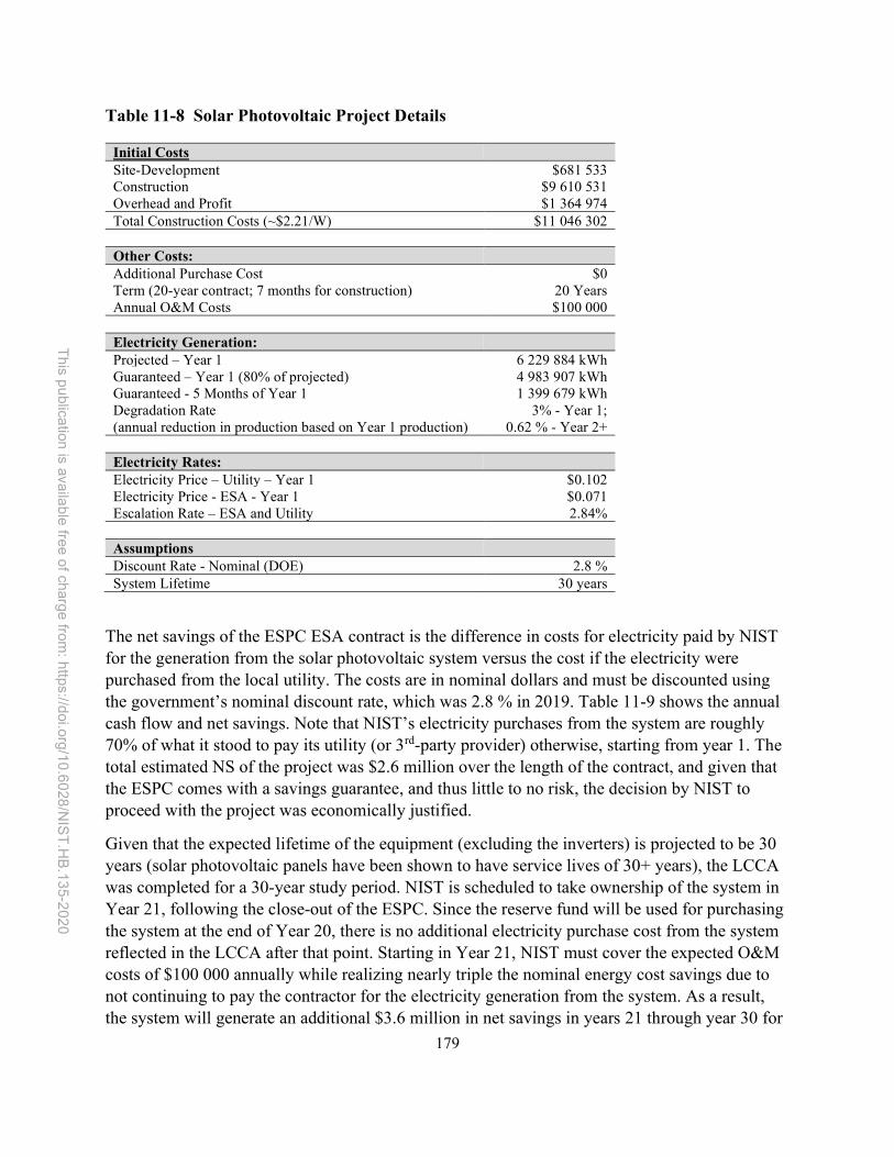
179

This p

ublica

tion is ava

ilab

le free

of ch

arge

from: h

ttps://doi.o

rg/1

0.6

028

/NIS

T.H

B.13

5-202

0

Table 11-8 Solar Photovoltaic Project Details

Initial Costs Site-Development $681 533 Construction $9 610 531 Overhead and Profit $1 364 974 Total Construction Costs (~$2.21/W) $11 046 302 Other Costs: Additional Purchase Cost $0 Term (20-year contract; 7 months for construction) 20 Years Annual O&M Costs $100 000 Electricity Generation: Projected – Year 1 6 229 884 kWh Guaranteed – Year 1 (80% of projected) 4 983 907 kWh Guaranteed - 5 Months of Year 1 1 399 679 kWh Degradation Rate (annual reduction in production based on Year 1 production)

3% - Year 1; 0.62 % - Year 2+

Electricity Rates: Electricity Price – Utility – Year 1 $0.102 Electricity Price - ESA - Year 1 $0.071 Escalation Rate – ESA and Utility 2.84% Assumptions Discount Rate - Nominal (DOE) 2.8 % System Lifetime 30 years

The net savings of the ESPC ESA contract is the difference in costs for electricity paid by NIST for the generation from the solar photovoltaic system versus the cost if the electricity were purchased from the local utility. The costs are in nominal dollars and must be discounted using the government’s nominal discount rate, which was 2.8 % in 2019. Table 11-9 shows the annual cash flow and net savings. Note that NIST’s electricity purchases from the system are roughly 70% of what it stood to pay its utility (or 3rd-party provider) otherwise, starting from year 1. The total estimated NS of the project was $2.6 million over the length of the contract, and given that the ESPC comes with a savings guarantee, and thus little to no risk, the decision by NIST to proceed with the project was economically justified.

Given that the expected lifetime of the equipment (excluding the inverters) is projected to be 30 years (solar photovoltaic panels have been shown to have service lives of 30+ years), the LCCA was completed for a 30-year study period. NIST is scheduled to take ownership of the system in Year 21, following the close-out of the ESPC. Since the reserve fund will be used for purchasing the system at the end of Year 20, there is no additional electricity purchase cost from the system reflected in the LCCA after that point. Starting in Year 21, NIST must cover the expected O&M costs of $100 000 annually while realizing nearly triple the nominal energy cost savings due to not continuing to pay the contractor for the electricity generation from the system. As a result, the system will generate an additional $3.6 million in net savings in years 21 through year 30 for

180

This p

ublica

tion is ava

ilab

le free

of ch

arge

from: h

ttps://doi.o

rg/1

0.6

028

/NIS

T.H

B.13

5-202

0

a total NS over the study period of $6.2 million. These net savings are obtained with no initial investment costs.

Table 11-9 ESPC Solar Photovoltaic Project Cash Flow and Net Savings

Year NIST Non-

Energy Costs ($) Guaranteed Gen. (kWh)

ESA Price ($/kWh)

Utility Rate ($/kWh)


PV Net Savings ($)

0 - - - - - -

1 - 1 399 679 0.071 0.102 42 997 41 826

2 - 4 855 416 0.072 0.103 150 749 142 649

3 - 4 825 329 0.074 0.106 153 989 141 746

4 - 4 795 242 0.076 0.109 157 379 140 921

5 - 4 765 154 0.078 0.112 160 908 140 156

6 - 4 735 067 0.08 0.115 164 091 139 036

7 - 4 704 980 0.082 0.118 167 866 138 360

8 - 4 674 894 0.085 0.121 171 277 137 326

9 - 4 644 806 0.087 0.125 175 250 136 685

10 - 4 614 719 0.09 0.128 178 842 135 687

11 - 4 584 632 0.092 0.132 182 967 135 036

12 - 4 554 545 0.095 0.136 186 693 134 033

13 - 4 524 458 0.098 0.14 190 923 133 336

14 - 4 494 371 0.100 0.144 195 186 132 600

15 - 4 464 284 0.103 0.148 199 023 131 525

16 - 4 434 197 0.106 0.152 203 319 130 704

17 - 4 404 110 0.109 0.156 208 054 130 105

18 - 4 374 022 0.112 0.161 212 331 129 163

19 - 4 343 936 0.115 0.165 217 016 128 417

20 - 4 313 849 0.119 0.170 221 657 127 591

21 100 000 4 287 966 - 0.175 649 656 363 771

22 100 000 4 262 238 - 0.180 666 321 362 940

23 100 000 4 236 664 - 0.185 683 356 362 081

24 100 000 4 211 244 - 0.190 700 770 361 194

25 100 000 4 185 977 - 0.196 718 571 360 281

26 100 000 4 160 861 - 0.201 736 767 359 343

27 100 000 4 135 896 - 0.207 755 368 358 381

28 100 000 4 111 081 - 0.213 774 383 357 395

29 100 000 4 086 414 - 0.219 793 820 356 387

30 100 000 4 061 896 - 0.225 813 689 355 357

Total PV Net Savings $6 204 030

It is beneficial to consider how this decision could be influenced by the “bonus” credit option for on-site production. The annual on-site production from the system (4 % of NIST’s annual consumption) counts double, which allows it to cover the 7.5 % statutory requirement assuming

181

This p

ublica

tion is ava

ilab

le free

of ch

arge

from: h

ttps://doi.o

rg/1

0.6

028

/NIS

T.H

B.13

5-202

0

NIST purchases a “REC swap” to replace the RECs that accrue to the ESCO through the ESA for the initial 20 years. There is no restriction on purchasing cheaper RECs (which are usually non-solar RECs) if available, which should lead to minimal costs for replacing the system’s RECs. For example, the Maryland solar RECs (aka SRECs) market – which is driven by the state’s ambitious “renewable portfolio standard” (RPS) – had prices ~ $50/MWh in 2019 while generic RECs (mostly from wind turbines elsewhere in the country, primarily in states without aggressive RPSs) generally were selling for < $1/MWh. The low price of these generic RECs is due to heavy and increasing wind production relative to the demand from the “voluntary” market (i.e., purchasers who choose to buy renewable electricity for environmental reasons). Assuming a price of $1 for the production in the initial 20 years, the additional present value cost would be $66 740 or ~1 % of the NS from the ESPC ESA.

There are several areas of uncertainty in this analysis that should be reviewed to ensure the results are not overly sensitive to the assumptions. First, the lifetime of the equipment could vary from the assumed 30 years. However, flawed solar panels typically fail relatively quickly (within the first few years) after installation, which would be covered by the equipment warranty from the manufacturer and handled by the ESCO per the contract agreement. The inverters are expected to last approximately 20 years. Depending on the exact year of failure or non-performance, either the ESCO (Year 1 through Year 20) or NIST will pay for the initial inverter(s) replacement. Additionally, there is the potential of a second replacement over Year 21 through Year 30. The initial cost of the inverters is $429 440, or ~ 4 % of the initial installed cost. In the worst-case scenario, NIST would replace the inverters twice at an estimated nominal cost of roughly $850 000, which would offset only a fraction of the total NS.

Second, production by the system may be over- or under-estimated. Solar panels degrade and/or fail at different rates. Higher (lower) degradation rates would lead to lower (higher) energy production. The solar panels and inverters include manufacturers’ performance warranties of 25 and 15 years, respectively, reducing concern of underproduction over the length of the contract. Additionally, the contract agreement guarantees only 80 % of the projected generation. Production estimates for the solar photovoltaic system have been accurate to actual production over the initial few months of operation, implying the system will more likely outperform versus underperform, and thus increase savings to NIST relative to the guaranteed value in the contract used for the calculations above.

Third, the electricity price paid to the local utility is likely going to escalate at different rates than the assumed 2.84 % constant rate because energy price escalations tend to diverge from expectations (and also not be linear over time). However, even under the assumption of zero nominal escalation of local utility energy prices, NIST would realize total net savings both over the contract ($764 000) and over the 30-year study period ($2.4 million). Note, though, that there would be some years (year 15 through year 20) in which NIST would not realize savings since the escalation rate on the payments to the ESCO would raise the price per kWh to a level higher than the local utility’s rate. Regardless, the project would realize non-trivial NS.

182

This p

ublica

tion is ava

ilab

le free

of ch

arge

from: h

ttps://doi.o

rg/1

0.6

028

/NIS

T.H

B.13

5-202

0

11.2.2 Example: On-Site Solar Photovoltaic System (Agency Funded)

Although NIST did not have resources to directly fund the project, it is beneficial to walk through that funding option to show how such an analysis could be completed. For this example, we use the same assumptions as those in Section 11.2.1 and assume that the installed costs of the solar system are the same as those provided by the ESCO ESA, excluding the mark-up (i.e., overhead and profit). If the installed costs provided in the proposal were paid for by NIST, the cash flow and net savings would be as shown in Table 11-10.

Table 11-10 Agency Funded Solar Photovoltaic Project Cash Flow and Net Savings

Year NIST Non-

Energy Costs ($) Guaranteed Gen. (kWh)

Utility Rate ($/kWh)

REC Value ($)


PV Net Savings ($)

0 10 221 062 - - - -10 221 062 -10 221 062 1 100 000 1 399 679 0.102 4572 47 047 45 766 2 100 000 4 855 416 0.103 4447 403 351 381 678 3 100 000 4 825 329 0.106 4326 414 255 381 319 4 100 000 4 795 242 0.109 4208 425 463 380 969 5 100 000 4 765 154 0.112 4094 436 968 380 613 6 100 000 4 735 067 0.115 3982 448 286 379 836 7 100 000 4 704 980 0.118 3874 460 358 379 441 8 100 000 4 674 894 0.121 3768 472 232 378 626 9 100 000 4 644 806 0.125 3666 484 836 378 144

10 100 000 4 614 719 0.128 3566 497 230 377 247 11 100 000 4 584 632 0.132 3469 510 330 376 640 12 100 000 4 554 545 0.136 3374 523 207 375 627 13 100 000 4 524 458 0.140 3282 536 767 374 865 14 100 000 4 494 371 0.144 3193 550 541 374 013 15 100 000 4 464 284 0.148 3106 564 075 372 769 16 100 000 4 434 197 0.152 3021 -280 626 -180 400 17 100 000 4 404 110 0.156 2939 593 062 370 866 18 100 000 4 374 022 0.161 2859 607 605 369 612 19 100 000 4 343 936 0.165 2781 622 753 368 508 20 100 000 4 313 849 0.170 2705 638 054 367 278 21 100 000 4 287 966 0.175 2632 654 356 366 403 22 100 000 4 262 238 0.180 2560 671 021 365 500 23 100 000 4 236 664 0.185 2490 688 056 364 571 24 100 000 4 211 244 0.190 2422 705 470 363 617 25 100 000 4 185 977 0.196 2357 723 271 362 638 26 100 000 4 160 861 0.201 2292 741 467 361 635 27 100 000 4 135 896 0.207 2230 760 068 360 610 28 100 000 4 111 081 0.213 2169 779 083 359 564 29 100 000 4 086 414 0.219 2110 798 520 358 497 30 100 000 4 061 896 0.225 2053 818 389 357 410

Total PV Net Savings $32 799

NIST could not have taken advantage of the investment tax credit (ITC, 30% of installed cost) or the accelerated depreciation tax benefit because federal agencies do not pay taxes. Assume the

183

This p

ublica

tion is ava

ilab

le free

of ch

arge

from: h

ttps://doi.o

rg/1

0.6

028

/NIS

T.H

B.13

5-202

0

value of the Maryland SRECs is not earned because NIST would retire the SRECs.28 In this case the bonus credit would be earned, doubling the 4 % to 8 % to meet and exceed the 7.5 % target.

Although the guaranteed generation is 4.9 million kWh (used for the economic evaluation), the predicted generation from the solar photovoltaic array is 6.2 million kWh (roughly 4 % of NIST’s total annual consumption in the late 2010s). Based on these estimates, 3.5 % of total consumption is 4.7 million kWh. Assuming NIST would have purchased RECs to meet its statutory requirement, it would have purchased RECs to cover this 4.7 million kWh (4700 RECs). Assuming $1 per REC, the present value cost savings from the “bonus” credit is $94 550. This could change if the value of REC prices were to increase significantly. The energy cost savings is the value of the electricity not purchased from the utility.

Based on these assumptions the NS is approximately $33 000, showing that funding the project with agency funds could have been cost-effective relative to purchasing electricity from the local utility. However, sensitivity analysis would likely show this outcome to be heavily dependent on numerous assumptions. The ESPC ESA leads to additional NS of $6.17 million and was, therefore, the better option for NIST versus using agency funding. The difference in NS can largely be accounted for by the ITC benefit, the estimated value of the SRECs at the time of the contract award, and the accelerated depreciation values.

28 Note that NIST could alternatively complete a REC “swap” in which the agency could sell the SRECs and then purchase replacement RECs, leading to potential savings if the value of the SRECs is higher than the value of the replacement RECs. This is excluded from the analysis for simplicity.

184

This p

ublica

tion is ava

ilab

le free

of ch

arge

from: h

ttps://doi.o

rg/1

0.6

028

/NIS

T.H

B.13

5-202

0

12 Evaluating Sustainability Projects

Sustainability is increasingly becoming a key driver in decision-making across all sectors of the U.S. economy. The construction sector has shifted over time from focusing on just energy efficiency (and associated dollar savings) towards greater interest in the broader goals of sustainability and higher overall performance. The broadening of the scope of criteria driving decisions has led to market expansion and job growth in the “green buildings” market. More broadly, demand for green and sustainable products and services have grown exponentially over the last decade, leading to over a million “green goods and services” jobs in the U.S. manufacturing and construction industries (Bureau of Labor Statistics, 2013). The green building segment of the U.S. market has grown from a market share of 2 % in 2005 (Gaskin, 2013) to accounting for 67 % of all projects in 2015 (McGraw-Hill Construction, 2017). To date, there are over 100 000 USGBC LEED projects completed or in progress worldwide (U.S. Green Building Council, 2017). Green construction spending rose from $151 billion in 2015 to $224 billion in 2018 (U.S. Green Building Council, 2015). Trends appear to be leading to a greater share of all new construction and major renovations pursuing green certification (such as LEED or ENERGY STAR®) or comparable criteria and performance.

12.1.1 Additional Value of Sustainable Buildings

As was discussed in Section 4.7, there are other benefits that may impact the economics of a project and should be incorporated into an LCCA to provide a complete evaluation, with sustainability projects providing an exceptional illustration. Sustainable buildings have been shown to provide value above and beyond the operational savings from energy efficiency, water conservation, and renewable energy production. GSA (2018) found that GSA’s high-performance buildings show reductions in their typical energy (23 %) and water use (28 %) as well as building operating expenses (23 %), and waste landfilled (9 %), along with increased occupant satisfaction (2 %) relative to its legacy building stock. Other benefits, discussed in Section 4.7, included higher productivity, rents, resale values, and occupancy rates.

The value of sustainable buildings can be looked at from the perspective of different market participants:

an employer who owns the building, an employer who rents office space in the building, a building owner who rents office space to tenants.

In the first case, the employer who owns the sustainable building may pay higher initial construction costs (particularly for those receiving the highest ratings – e.g., LEED Gold or Platinum), but has savings associated with reduced energy costs and possibly higher worker productivity over the lifetime of the building, as well as higher resale values. In the second case, the employer most likely pays a higher rent, but enjoys reduced energy costs (assuming a net lease) and possibly higher worker productivity over the lease. Lastly, the building owner who

185

This p

ublica

tion is ava

ilab

le free

of ch

arge

from: h

ttps://doi.o

rg/1

0.6

028

/NIS

T.H

B.13

5-202

0

rents the building pays the slightly higher first cost to build or buy the building but receives higher rental values and occupancy rates.

The higher premiums are a result of some combination of lower operational savings (e.g., from lower energy, water, operations, maintenance, repair and replacement costs) and better indoor environmental quality (IEQ), which has been shown to improve worker productivity and occupant wellbeing, reduce employee turnover, and help attract and retain employees. Although achieving basic (lower) levels of sustainable building certification (e.g., “LEED certified”) does not explicitly require achieving high IEQ, higher levels of sustainable building certification (e.g., LEED Gold and Platinum) do specify improved IEQ by meeting building ventilation standards as well as through evaluating the perceptions of building occupants. Higher employee perception of IEQ is correlated with higher productivity, which can justify higher rent prices.

Given the information provided above:

Renting office space in a sustainable building and paying a higher rent premium may still be cost-effective.

For employer-owned buildings, an additional capital cost for sustainable building design and construction may be offset by cost savings over a 40-year (or shorter) study period length.

Profitability for a building owner who constructs a sustainable building and rents it to multiple tenants may be higher depending on the market.

Specific requirements for IEQ performance and methods of testing it will need to be included in contract language to assure that parameters and technologies contributing to higher worker productivity and well-being are implemented.

12.1.2 Federal Sustainable Building Guidance and Requirements

Since 2006, multiple executive orders have recognized high performing, sustainable buildings as a key component in efforts to reduce environmental impacts, cut GHG emissions, and lower operating costs at federal facilities (CEQ, 2016). The Council on Environmental Quality developed the first guidance on building performance goals (specifically, reducing energy and water use, conserving resources, minimizing waste, protecting indoor air quality, and requiring integrated design) for federal facilities through its “Memorandum of Understanding for Federal Leadership in High Performance and Sustainable Buildings” in 2006 (CEQ, 2006). The guiding principles were updated in 2008 (CEQ, 2008) in “High Performance and Sustainable Buildings Guidance,” and then again in “Guiding Principles for Sustainable Federal Buildings and Associated Instructions” (CEQ, 2016). This most recent guidance was updated to reflect the evolution of sustainable building design, construction and operating practices, as well as to increase economic and environmental benefits of federal investments in facilities, enhance occupant health, wellness, and productivity, include climate resilience, and assist in tracking these performance goals. The guidance is to be applied wherever it is deemed life-cycle cost-effective, following benefit-cost analysis in accordance with OMB Circular A-94 (OMB, 2018a) and OMB Circular A-11 (OMB, 2018b). The LCC methodology defined in this handbook is consistent with both circulars. Table 12-1 shows the metrics defined for new construction,

186

This p

ublica

tion is ava

ilab

le free

of ch

arge

from: h

ttps://doi.o

rg/1

0.6

028

/NIS

T.H

B.13

5-202

0

modernization (improving functionality, energy performance, and aesthetics), and existing buildings.

Table 12-1 Sustainable New Construction and Modernization Guidance (CEQ, 2016)

Category Metric Required Categories

New Modern. Existing* Employ Integrated Assessment, Operation, & Management

Integrated Assessment, Operation, & Management

X X X

Commissioning X X X

Optimize Energy Performance

Energy Efficiency X X X

Renewable and Clean Energy X X

Metering X X

Benchmarking X X

Protect and Conserve Water

Indoor Water Use X X X

Outdoor Water Use X X

Alternative Water X X

Stormwater Management X X

Enhance Indoor Environmental Quality

Ventilation and Thermal Comfort X X X

Daylighting and Lighting Controls X X

Indoor Air Quality X X

Occupant Health and Wellness X X

Reduce Environmental Impact of Materials

Material Content and Performance X X X

Waste Diversion X X X

Materials Management X X

Assess and Consider Climate Change Risks

Mission Criticality X

Floodplain Considerations X

Facility Design X

Facility Adaptation X

Climate Resilience and Adaptation X

* Requires a minimum of 4 optional metrics along with the 8 required.

187

This p

ublica

tion is ava

ilab

le free

of ch

arge

from: h

ttps://doi.o

rg/1

0.6

028

/NIS

T.H

B.13

5-202

0

In some cases, the sustainability metrics could be evaluated individually. However, there may be interactions across the different criteria/goals, which could require evaluating across different metrics at the same time. Since sustainable buildings are measured across multiple performance criteria, attention should be placed on the specific goals of the project. The goals will determine the constraints and minimum requirements, appropriate discount rate, and determine the benefits and costs that should be included in a project analysis. For example, a goal of reducing GHG emissions could either be a minimum requirement (e.g., specified target of 30% reduction) or a variable for optimization (e.g., maximum reduction for a given cost). Additionally, there may be minimum requirements under other criteria, such as resilience. The appropriate discount rate to use will depend on whether the GHG emissions reductions are obtained from ECMs or other approaches, such as reducing embodied emissions in building materials. As was discussed in Section 2.2.3, if a project involves energy usage only peripherally, and the energy- (including water) related and non-energy-related parts of the investment cannot be broken out, the decision as to whether to use OMB Circular A-94 criteria or FEMP criteria is left to the judgment of the analyst. The benefits and costs associated with the GHG reduction that should be included in the analysis will be dependent on the baseline case, which will be different depending on whether the GHG reduction is a minimum requirement or optimization.

EO 13834 states and CEQ (2019b) reasserts that at least 15 % of federally owned buildings greater than 10 000 ft2 (either number of buildings or gross area) must qualify as sustainable, with demonstration of annual progress. Agencies can either use these guiding principles or 3rd party certification systems or standards that meet the certification standards established in 10 CFR 433 and 10 CFR 435 Subpart C. In 2013, the two certification programs identified as the best suited to meet these requirements were the Green Building Initiative’s Green Globes and the USGBC’s LEED. New guidance is forthcoming that could expand the list of best suited certification programs based on a 2019 review of current high-performance certification systems (Bower, Bryan, Canada, Carter, & Watts, 2019).

Figure 12-1 shows that the fraction of federal buildings and gross floor area that qualify as sustainable rose from 1.0 % and 3.5 %, respectively, in 2010 to 6.7 % and 10.4 % in 2018. These results are for the entire building stock owned or leased by the federal government. When using the same underlying dataset, ~20 % of all federally owned gross floor area qualified as sustainable in FY2018. Federally leased buildings, which account for ~50 % of area and ~80 % of the number of buildings, are exempt from the 15 % requirement. However, all federally leased buildings must be ENERGY STAR certified. Additionally, federally leased buildings should be sustainable “if cost-effective.” CEQ (2019b) also states that agencies should optimize space utilization in owned and leased buildings. GSA is responsible for most non-military federally owned or leased properties (Veteran’s Affairs (VA) and DOE also oversee significant facilities). According to GSA’s Inventory of Owned and Leased Properties (IOLP) (as of June 2019), GSA owns and/or leases ~376 million ft2 of space in ~9400 buildings. Among its owned space are154 green building certifications covering 44.6 million ft2, or 24 % of the GSA portfolio by area (GSA, 2019).

188

This p

ublica

tion is ava

ilab

le free

of ch

arge

from: h

ttps://doi.o

rg/1

0.6

028

/NIS

T.H

B.13

5-202

0

Figure 12-1 Federal Government High Performance Sustainable Buildings (CEQ, 2019a)

12.1.3 Example: Building Life-Cycle Sustainability Analysis

The example below is based on the analysis conducted by GSA (2012) that develops a “composite” LCCA that combines LCCA and LCA (discussed in Section 4.7.3). LCA is typically a “mid-point” analysis, providing a quantity for environmental impacts (e.g., carbon emissions) instead of a monetary value to the resulting societal costs (e.g., social cost of carbon). However, GSA (2012) combines the LCA results with a range of estimates for the externality costs from environmental impacts.

Note that each LCCA analysis is unique and should use the best available information and data available for the specific situation being analyzed. The data in this example can be traced back to its original sources to determine if it is representative of a reader’s decision. A reader should also consider other studies that have been published since this report’s release in 2012 that may be more appropriate.

189

This p

ublica

tion is ava

ilab

le free

of ch

arge

from: h

ttps://doi.o

rg/1

0.6

028

/NIS

T.H

B.13

5-202

0

Table 12-2 shows that the study considers three GSA buildings (Fallon, Garmatz, and Custom House) in Baltimore, Maryland across which 24 sustainability measures were considered for implementation, ten focused on GSA Sustainable Guidelines and LEED credits and 14 that were building-specific measures. The sustainability measures consider the following LEED categories: sustainable site, water efficiency, energy and atmosphere, materials and resources, and indoor environmental quality.

The LCA impact categories selected for analysis were from the TRACI characterization methods (Environmental Protection Agency, 2018): GWP, acidification potential, ozone depletion potential, eutrophication potential, human health – respiratory effects (i.e., criteria air pollutants), and photochemical smog formation. Given the focus of this handbook, the detailed LCA analysis is not discussed. The LCA results are assumed to have been developed correctly and consistent with all appropriate standards, particularly those from the International Standards Organization (ISO).

190

This p

ublica

tion is ava

ilab

le free

of ch

arge

from: h

ttps://doi.o

rg/1

0.6

028

/NIS

T.H

B.13

5-202

0

Table 12-2 Sustainability Measure NPV for 3 Building Project

Measure Primary Target Building

1. Enable Water-Side Economizer Energy Fallon

2. Repair Glycol Run-Around Loop Energy Fallon

3. Lighting Retrofits Energy Garmatz

4. Reduce Plug Loads Energy Garmatz

5. Install Heat Pipe Energy Custom House

6. Air Handling Unit Replacement Energy Fallon

7. Air Handling Unit Replacement Energy Custom House

8. Co-Generate Electricity Energy Garmatz

9. Replace Windows Energy Custom House

10. Green Roof Energy Custom House

11. Deep Energy Retrofit—Replace Windows Energy Fallon

12. Deep Energy Retrofit—GSHP Energy Fallon

13. Cool Roof Energy Garmatz

14. Solid Waste Management Environmental Multiple

15. Mercury in Lighting Environmental Multiple

16. Refrigerant Management Environmental Multiple

17. Green Cleaning Environmental / Health Multiple

18. Indoor Air Quality Health Multiple

19. Off-Site Renewable Energy Renewable Energy Garmatz

20. On-Site Renewable Energy Renewable Energy Fallon

21. Deep Energy Retrofit—Add Photovoltaics Renewable Energy Fallon

22. Transportation Transportation Multiple

23. Indoor Water Use Water Garmatz 24. Landscaping Water Multiple

The unit of measure for each impact category is different, which makes it difficult to compare the LCA results. Therefore, the LCA results have been converted from non-monetary environmental impact values to monetary values using data from numerous studies to determine the externality costs of pollution (i.e., costs not internalized in the price of the building). Table 12-3 is a re-creation of GSA’s table GSA (2012) for externality costs ($/ton) by impact category developed for this example.

191

This p

ublica

tion is ava

ilab

le free

of ch

arge

from: h

ttps://doi.o

rg/1

0.6

028

/NIS

T.H

B.13

5-202

0

Table 12-3 Externality Costs by Impact Category

Impact Category Unit Low Mid High

GWP t CO2-eq $1 $30 $100

Ozone Depletion t CFC-11-eq $5500

Impact Category Unit Percentile

1st 25th 50th 75th 99th 99.9th

Acidification t H+-eq $1 $3 $9 $21 $22 $593

Eutrophication t N-eq $6 $52 $73 $107 $319 $516

Smog t NOX-eq $32 $95 $142 $221 $1080 $3580

Respiratory Effects t PM2.5-eq $250 $700 $1170 $1970 $12 400 $41 770

Table 12-4 re-creates GSA’s estimated externality costs of electricity table (GSA, 2012) for each of the impact categories using the bolded values (either midpoint or 99th percentile) in Table 12-3. The per unit estimated externality costs are not necessarily indicative of the total externality costs because the magnitude of impacts vary significantly across impact categories. Nearly all the externality cost from electricity consumption is a result of GWP ($19.10/MWh) and respiratory effects ($16.00/MWh) followed by acidification potential ($4.90/MWh) while the other impact categories have minimal economic value ($0.20/MWh in total).

Table 12-4 Electricity Externality Costs by Impact Category

Impact Category Impact from 1 MWh

External Cost

$/kg $/MWh $/kWh

GWP (kg CO2-eq) 6.37 E+02 $0.03 $19.10 $0.02

Ozone Depletion (kg CFC-11) 1.69 E-10 $55.00 <$0.05 $0.00

Acidification (moles H+-eq) 2.30 E+02 $0.02 $4.90 $0.00

Eutrophication (kg N-eq) 5.65 E-03 $0.32 <$0.05 $0.00

Smog (kg NOX-eq) 1.05 E-01 $1.08 $0.10 $0.00

Respiratory Effects (kg PM2.5-eq) 1.29 E-00 $12.40 $16.00 $0.02

Total NA $40.20 $0.04

*Note: sum of the columns may not match due to rounding.

192

This p

ublica

tion is ava

ilab

le free

of ch

arge

from: h

ttps://doi.o

rg/1

0.6

028

/NIS

T.H

B.13

5-202

0

The approach in calculating the externality costs of electricity was replicated for other fuel types as shown in Table 12-5, which re-creates GSA’s estimated externality costs of other fuels (GSA, 2012). These values are used to estimate the energy-related externality costs or cost savings from implementation of the 24 sustainability measures considered in this example.

Table 12-5 Externality Costs of Other Fuel Types

Fuel Type Unit Externality Cost

Electricity – Maryland 1 MWh $39.83

Electricity – US Average 1 MWh $30.96

Steam – Baltimore - 60 % MSW, 40 % natural gas 1 short ton $10.04

Steam - 100 % natural gas 1 short ton $11.36

Chilled Water – Baltimore 1000 ton-hours $48.11

Chilled Water – US Average 1000 ton-hours $47.53

Fuel Oil 1000 L (264 gal) $97.70

Table 12-6 shows the net present value savings from the LCCA, the externality cost savings, and the “composite” net savings when combining the two. Of the 24 measures, twelve are LCC cost-effective when considering the direct costs only while sixteen are cost-effective once the externality costs are included in the LCCA. Many of the measures with the highest initial costs had significant negative net savings both with and without externality costs: ground source heat pump, green and cool roofs, window replacements, and on-site solar photovoltaics. Eleven measures are cost-effective regardless of whether externalities are included in the LCCA. Five measures that were not LCC-effective using direct costs only become cost-effective once the externalities are included, including the three measures with the largest externality cost savings (off-site renewable energy, transportation, and indoor air quality). One measure that was cost-effective is no longer so once the externalities are included (DER-ground source heat pump).

Note that this analysis treats each measure independently. As has been shown in this handbook, there may be interactions across different measures within the same facility. However, this analysis assists in narrowing down the potential sustainability measures to consider. The analysis also shows how the inclusion of externalities can impact the decision, and in some cases externalities (or other non-direct or non-monetary benefits and costs) can dominate the LCCA. The details of the steps in the LCCA process completed in the example are not reported here. For more details, see GSA (2012).

193

This p

ublica

tion is ava

ilab

le free

of ch

arge

from: h

ttps://doi.o

rg/1

0.6

028

/NIS

T.H

B.13

5-202

0

Table 12-6 Sustainability Measure NPV for 3 Building Project

Measure Direct NPV Externality NPV

Composite NPV

Building

1. Off-Site Renewable Energy ($64 090) $3 239 106 $3 175 016 Garmatz

2. Enable Water-Side Economizer $862 021 $210 316 $1 072 337 Fallon

3. Transportation ($516 995) $1 493 860 $976 865 Multiple

4. Indoor Air Quality ($40 043) $953 633 $913 590 Multiple

5. Repair Glycol Run-Around Loop $388 589 $156 471 $545 060 Fallon

6. Landscaping $368 339 $30 $368 369 Multiple

7. Lighting Retrofits $166 627 $153 501 $320 128 Garmatz

8. Reduce Plug Loads $97 478 $59 932 $157 410 Garamtz

9. Solid Waste Management $36 810 $89 625 $126 435 Multiple

10. Install Heat Pipe $19 639 $23 897 $43 536 Custom House

11. Indoor Water Use $23 446 $17 707 $41 153 Garmatz

12. Mercury in Lighting $20 792 $5 $20 797 Multiple

13. Air Handling Unit Replacement ($50 882) $68 236 $17 354 Fallon

14. Air Handling Unit Replacement ($2 482) $15 229 $12 747 Custom House

15. Green Cleaning $1438 $60 $1498 Multiple

16. Refrigerant Management $74 $522 $596 Multiple

17. Co-Generate Electricity ($243 578) $182 026 ($61 552) Garmatz

18. Replace Windows ($236 959) $168 677 ($68 282) Custom House

19. On-Site Renewable Energy ($139 199) $50 447 ($88 752) Fallon

20. Deep Energy Retrofit—Add Photovoltaics ($139 199) $50 447 ($88 752) Fallon

21. Green Roof ($295 405) ($1 717) ($297 122) Custom House

22. Deep Energy Retrofit—Replace Windows ($1 922 150) ($64 002) ($1 986 152) Fallon

23. Deep Energy Retrofit—GSHP $40 ($3 913 067) ($3 913 027) Fallon

24. Cool Roof ($4 962 505) $23 278 ($4 939 227) Garmatz

194

This p

ublica

tion is ava

ilab

le free

of ch

arge

from: h

ttps://doi.o

rg/1

0.6

028

/NIS

T.H

B.13

5-202

0

13 Evaluating Resilience Projects

As was discussed in Section 9.4, resilience is the ability to prepare for, withstand, and recover from disruptions caused by major accidents, attacks, or natural disasters.” Another common definition of resilience is “the ability for optimized operations to withstand, adapt, and recover from disruption.” Resilience projects can target any or all three areas. For example, assume that a facility faces regular power outages due to an unreliable electric grid. To “withstand” a disruption, a facility may include back-up generators to operate when utility power is unavailable. Resilience through the ability to “adapt” to a disruption could include a more robust on-site power generation system that can transition to and from different power resources. Greater ability to “recover” from a disruption could be accomplished by smart buildings that can provide detailed information to facility managers with information on power outages to accelerate restoration of power to occupants. The area(s) of resilience to target depends on the specific facility and the agency’s mission and goals associated with the project.

Projects that improve resilience can be combined with energy and water conservation measures to leverage those activities, and in some cases the measures have co-benefits, providing both recurring resource conservation and better resilience to potential disruptions in the future (e.g., on-site generation with energy storage). Depending on the goal of the project, the factors over which to optimize may change. A project may want to minimize LCC while reaching some level of resilience, in which case resilience is an underlying constraint. Alternatively, a project may be trying to minimize expected LCCs, in which case the level of resilience may vary depending on the relative benefits and costs. The approach to setting up and analyzing the decision will change depending on the constraints and goals of the analyst.

This chapter provides just a few examples of the types of resilience-related projects facing government agencies, including both infrastructure and energy resilience projects. The analysis in the examples may consider a wider scope than just a single building or facility, but the examples are still relevant in understanding the analysis process of considering a multifactor optimization problem such as resilience.

13.1 Evaluating Infrastructure Resilience Projects

Gilbert et al. (2015) provides several community resilience projects, providing a broader perspective than a single building, facility, or campus. Although some of the guide is outside the scope of projects that are a focus of this handbook, the information and examples provided in the guide and the associated standard can assist users of this handbook when determining the considerations of incorporating resilience-related benefits and costs in their economic analysis.

13.1.1.1 Example: Bridge Retrofit versus Replacement

Appendix A in Gilbert et al. (2015) focuses on a decision regarding retrofitting an existing bridge to meet minimum performance specifications or replacing the existing bridge with a new one in a fictional Riverbend, USA. The benefits and costs under consideration range from the direct

195

This p

ublica

tion is ava

ilab

le free

of ch

arge

from: h

ttps://doi.o

rg/1

0.6

028

/NIS

T.H

B.13

5-202

0

construction-related costs to reduced damages from natural disasters to recurring benefits to motorists and residents. The following is adapted from that example.

Problem Setup: The four-lane interstate bridge over the Central River between Riverbend and neighboring Fallsborough is the only crossing for traffic and clean water distribution into Riverbend. The traffic volume is currently higher than the design capacity, operating below driver expectation during peak hours while serving as the main link for emergency vehicles including fire and rescue (high potential negative impacts from disruptions). This structure is sensitive to both river flooding and seismic events (low resilience performance), and therefore, there are high expected negative impacts from a weather-related shock.

Two alternate plans to improve community resilience are considered, both designed to increase resilience from flooding and earthquakes to reduce economic losses and loss of life should a disaster occur. The second plan is expected to ease traffic congestion during peak hours while further reducing potential impacts from seismic activity.

Baseline Alternative: Retrofit the Central River bridge to eliminate flooding-related disruptions and a seismic rehabilitation to lower damage from an earthquake. Existing bridge cannot be brought up to seismic code.

Since the existing bridge is scheduled (and budgeted) to undergo a deck replacement in ten years, there was an opportunity to complete a seismic upgrade that would also create greater resilience against flood conditions but not eliminate potential damage from a seismic event. Deck replacement requires closing the bridge, forcing a longer route for emergency services and regular traffic. The user cost of the longer drive from the detour and the deterioration of alternate route roads are losses that should be considered.

Alternative 1: Construct a second bridge over the Central River consistent with seismic codes.

The new bridge could be built in an offset alignment while maintaining the traffic on the existing bridge. The new bridge will withstand a seismic event and maintain traffic. This second crossing would relieve congestion during high traffic periods when traffic volume exceeds the capacity of the existing bridge and provide additional water supply that would benefit Riverbend’s long-term development plans. The new bridge would meet the seismic, redundancy, and strength requirements and would be designed to last 125 years. Also, the new bridge would allow for the traffic to be shifted when replacement of the existing bridge was required. In addition, it would include a non-motorized path to enhance quality of life for city residence.

In this example, the bridge must meet minimum resilience requirements to reduce impacts from flooding as represented on the lower portion of the y-axis in Figure 13-1. Therefore, the current bridge without a retrofit (B.L.) is not a feasible alternative. The rehabilitation of the existing bridge is considered the baseline because it has the lowest initial direct costs (B.C.). Constructing a new bridge is the alternative being considered (Alt. 1), which provides resilience performance that exceeds the minimum required resilience. The upper portion of Figure 13-1 shows the incremental benefits and costs of the alternatives. The costs for Alt. 1 are higher than for B.C.,

196

This p

ublica

tion is ava

ilab

le free

of ch

arge

from: h

ttps://doi.o

rg/1

0.6

028

/NIS

T.H

B.13

5-202

0

but the benefits (expected reduction in costs associated with damages from flooding and earthquakes and lower negative impacts on the residence) are higher for Alt. 1. Completing a LCCA just focused on the direct benefits and costs would miss most of the impacts on the community.

Figure 13-1 Resilience-Related Retrofit

The assumptions for the analysis are provided in Table 13-1 while the benefits and cost results are shown in Table 13-2. The alternative with greater (positive) present value net benefit (or lowest present value net costs) is the optimal selection.

Table 13-1 Bridge Resilience Project Summary29

Assumptions Values Discount Rate 5 % Study Period 50 years Statistical Value of a Life $7.5 million Disaster Recurrence 25 years (4 % annual probability) Disaster Magnitude Direct Damage 1/16 replacement costs Risk Preference Risk Neutral

29 Note that the disaster magnitude and risk preference are not used in Gilbert et al. (2015).

197

This p

ublica

tion is ava

ilab

le free

of ch

arge

from: h

ttps://doi.o

rg/1

0.6

028

/NIS

T.H

B.13

5-202

0

Alternative 1 leads to an expected value of net benefits of $1.5 million. The expected present value net benefit of the baseline was lower, and negative (-$0.8 million). In other words, alternative 1 leads to expected net present value savings of $2.3 million relative to the Baseline.

Table 13-2 Bridge Resilience Project Results

Present Expected Value Baseline Alternative 1

Benefits Disaster Economic Benefits

Response & Recovery Costs $449 007 $748 344 Direct Losses $194 570 $0

Indirect Losses $1 496 689 $2 619 206

Disaster Non-Market Benefits Lives Saved $561 258 $1 122 517

Non-Disaster Related Benefits

Reduced Commute Time $0 $1 825 593

Costs Initial

Direct $3 000 000 $4 250 000 Indirect $500 000 $50 000

Decadal Cost $0 $507 711 Residual Value $0 $0

Total Present Expected Value Benefits $2 701 524 $6 315 660 Costs $3 500 000 $4 807 711 Net ($798 476) $1 507 949 Expected NS $2 306 425

For simplification of the example, discussion of the probability and results distributions are excluded. Additional information on this example can be found through Gilbert et al. (2015). An expansion of this example is available in the Economic Decision Guide Software (EDGe$) user guidance (Helgeson, Webb, & Grubb, 2017).

13.2 Evaluating Energy Resilience Projects

Assessing energy resilience requires a vulnerability assessment that includes the following steps (FEMP, 2006):

Create or update energy system descriptions, including energy feeds/deliveries to the site.

198

This p

ublica

tion is ava

ilab

le free

of ch

arge

from: h

ttps://doi.o

rg/1

0.6

028

/NIS

T.H

B.13

5-202

0

Identify critical facilities and associated loads based strictly on the site’s mission and/or function.

Identify critical energy requirements from on-site sources and off-site energy feeds.

Identify all significant potential threats from natural phenomena, fires, accidents, equipment failure, and intentional causes.

Perform a probabilistic vulnerability analysis for all identified threat scenarios.

Derive both a best estimate and a maximum estimate of impact duration for all viable threat scenarios while considering the availability of repair crews in each case.

Based on the results of the probabilistic vulnerability analysis, list unacceptable risks to be addressed by the remedial action plan.

For some agencies and facilities, this process may be relatively straightforward while others may require a much more complex process to assess current and future vulnerabilities. Threats to energy security can include natural phenomena (e.g., earthquakes, floods, hurricanes, tornadoes, extreme heat, ice storms), site-specific threats (e.g., fire, accidents, facility equipment or system failures), and intentional threats (labor strikes or contract defaults, sabotage, terrorism, or riots, arson and vandalism, and cyber attacks) (FEMP, 2006).

To assist resilience projects focused on renewable energy, DOE has funded NREL to develop the Renewable Energy Integration and Optimization (REopt) tool. REopt (https://reopt.nrel.gov/) is a “techno-economic decision support model used to optimize energy systems for buildings, campuses, communities, and microgrids.” REopt recommends an optimal mix of renewable energy, conventional generation, and energy storage technologies to meet cost savings and energy performance goals (NREL, 2019c). REopt has supported decisions in renewable energy screening, campus planning, microgrid development, resiliency, and others, leading to over 260 MW of renewable energy deployment (https://reopt.nrel.gov/). A free version of REopt with a subset of the full tool’s features, REopt Lite (https://reopt.nrel.gov/tool), is a web tool that can help commercial building managers evaluate the economic viability of grid-connected photovoltaics, wind, and battery storage at a site, identify system sizes and battery dispatch strategies to minimize energy costs, and estimate how long a system can sustain critical load during a grid outage (NREL, 2019b).

Many Department of Defense (DoD) facilities are in areas in which access to energy and water may be limited, unreliable, and/or costly, making resource access and conservation a top priority. For FY2015, DoD directly invested $500 million in conservation and energy efficiency, with $350 million for sustainment and recapitalization (i.e., retrofit projects that may include conservation measures) and $150 million as part of its Energy Conservation Investment Program (ECIP) to directly fund conservation construction projects (energy efficiency, water conservation, and renewable energy) (GAO, 2016). Alternative funding through ESPCs (5-year average of $430 million) and UESCs (5-year average of $69 million) are also common mechanisms implemented according to the Annual DoD Energy Management Reports (DoD, 2019).

199

This p

ublica

tion is ava

ilab

le free

of ch

arge

from: h

ttps://doi.o

rg/1

0.6

028

/NIS

T.H

B.13

5-202

0

Military installations must complete LCCA to assess long-term cost-effectiveness of projects based on MILCON and Department of Defense Instruction (DoDI) 4170.11 requirements (DoD, 2018). As discussed in Section 1.3, MILCON projects must use LCCA and implement a mid-year discounting method. DoDI 4170.11 (consistent with this handbook) requires the use of LCCA for energy efficiency, water conservation, and renewable energy investment decisions as well as energy resilience projects. All projects with ten years or less SPB that meet financial constraints are supposed to be implemented. Projects with higher SIR are supposed to be pursued using alternative financing mechanisms (e.g., ESPCs and UESCs).

Projects funded through ECIP have to be cost-effective (SIR > 1, with the overall portfolio of each year’s projects having an SIR > 2.0), and evaluated based on the following criteria (DoD, 2015):

(1) Service priority (2) Part of an energy plan (3) Demonstration of a test bed or other innovative technology (4) Integration of multiple technologies to realize synergistic benefits (5) Contribution to energy efficiency, renewable energy, and water conservation goals

The National Defense Authorization Act (NDAA) for FY2017 changed 10 USC § 2914 to prioritize facility resiliency in current efforts to improve operations by redesigning the ECIP to become the Energy Resilience and Conservation Investment Program (ERCIP). The new evaluation criteria have been expanded to include improved energy resilience, security, availability, and reliability, in conjunction with economic performance. Consistent with this, the ranking system uses a multi-objective function based on the following order of priorities (DoD, 2017a):

(1) Improves energy resilience and contributes to mission assurance (2) Service priority (3) Net present value (4) Part of an energy plan (5) Demonstrates test bed or other innovative technology (6) Integrates multiple technologies to realize synergistic benefits (7) Contributes to energy efficiency, renewable energy, and water conservation goals

Additional project portfolio constraints on ERCIP include (DoD, 2017a):

(1) Project portfolio should strive to maximize SIR (2) Energy resilience/security projects must enhance mission assurance, support mission critical

functions, address vulnerabilities, and be cost-effective (3) Portfolio should align with target funding allocation of 50 % energy resilience/security, 25 %

energy efficiency, 15 % renewable energy, and 10 % water conservation

200

This p

ublica

tion is ava

ilab

le free

of ch

arge

from: h

ttps://doi.o

rg/1

0.6

028

/NIS

T.H

B.13

5-202

0

Energy resilience has been defined as “…the ability to avoid, prepare for, minimize, adapt to, and recover from anticipated and unanticipated energy disruptions in order to ensure energy availability and reliability sufficient to provide for mission assurance and readiness” (10 U.S.C. § 101, 2011). Resilience in DoD installations must balance flexibility, reliability, and resistance with honest acknowledgement of resource constraints to be as effective as possible (Baxter, 2018).

By prioritizing energy resilience in ERCIP projects, military installations must identify the energy requirements that are mission-critical, prioritize the critical loads, and evaluate alternative solutions to provide the necessary energy resilience for those loads under potential scenarios. Resilience efforts can include projects that do not immediately impact energy use, such as burying power cables, building flood walls around equipment, raising mounting levels, or installing equipment inside buildings. Other projects that improve resilience may also lower or shift electricity demand, such as on-site renewable production, energy storage, or installing more efficient heating and cooling equipment. These potential synergies between energy resilience and energy efficiency, water conservation, and renewable energy projects may lead to more cost-effective options by leading to regularly gained “co-benefits” (e.g., lower electricity costs) while increasing resistance to potential outages.

The evaluation process could vary significantly across installations due to the unique energy resilience constraints for each situation. Utility outages at DoD facilities are primarily from routine (e.g., end-of-life) equipment failure (45 %) and planned maintenance (39 %), with acts of nature causing all but 2 % of the remaining 17 % (Castillo, 2017). Relatively minor efforts may be needed to provide better resilience under equipment failure or scheduled maintenance, such as uninterruptible power supplies or back-up generators. However, many installations may be required to be designed to provide higher levels of energy resilience under more uncommon scenarios, such as extreme weather events or human actions, that require extended periods of off-grid operation (e.g., on-site renewable production and energy storage).

Meeting energy resilience goals while striving to comply with DoD’s other objectives for ERCIP projects (see above) quickly complicates the evaluation process. To assist evaluating resilience projects, DoD funded Massachusetts Institute of Technology Lincoln Laboratories (MIT-LL) to develop the Energy Resilience Assessment (ERA) tool.30 These tools assist in analyzing the cost-effectiveness of energy resilience and energy security projects consistent with Circular A-94 (Judson, Pina, Dydek, Broekhoven, & Castillo, 2016).

During the development of ERA, some high-level recommendations were identified (Savena, Judson, & Pina, 2017). Resilient energy system design should be driven by mission requirements to ensure indifference to technology choice. A more flexible electric delivery system with centrally aggregated generation assets that can shift generation and load will have higher resilience. Systems should be designed and tested for typical operation as well as short- and long-term disruptions to evaluate how well they perform.

30 ERA is based on Matlab (back-end) and Excel (front-end).

201

This p

ublica

tion is ava

ilab

le free

of ch

arge

from: h

ttps://doi.o

rg/1

0.6

028

/NIS

T.H

B.13

5-202

0

Regardless of the complexity of the decision, the process remains the same for evaluating energy resilience project alternatives. The base case should generally be based on either the (1) lowest upfront cost option or (2) option that uses the most “traditional” method to address the resilience issue. All alternatives, including the base case, must meet or exceed the minimum level of energy resilience required based on the prioritization of critical loads to meet mission critical needs on an installation. For example, there may be a requirement to provide emergency generation and storage systems with appropriate redundancy to handle a defined common threat (e.g., level 3 hurricane force winds) while providing the capacities to meet minimum requirements specified by a federal agency (e.g., maintain normal operation). Alternatives may include both systems servicing individual mission-critical operations (distributed system solutions, such as building-specific generators) as well as solutions (e.g., a campus-wide microgrid) that address clusters of operational needs. Life-cycle cost analysis of energy resilience projects requires the consideration of the costs associated with all energy-related systems that may be impacted, including power and thermal energy systems to facilities served throughout the year across all potential modes of operation (i.e., non-emergency, emergency and testing).

The remainder of this section will provide examples of LCCA of energy resilience projects based on use cases published using ERA (Savena et al., 2017) and REopt (NREL, 2019c).

13.2.1 Example: Energy Resilience Project – REopt

This example is based on a study using REopt to evaluate economic and resiliency impacts of photovoltaics and storage on a facilities in New York City(Anderson et al., 2016). The study was completed as an effort to determine potential solutions to issues with long power outages that occurred during and after Superstorm Sandy hit New York, including at critical infrastructure such as hospitals, emergency response, and storm shelters. A lack of back-up power generators was one reason for these long outages. Anderson et al. (2016) evaluates alternative systems to minimize outages and maintain the critical infrastructure for the city in the case of another extreme weather event for three facilities: a high school/coastal storm shelter, a fire station, and a cooling center. The example below focuses on the fire station evaluation. See Anderson et al. (2016) for additional details on all facilities evaluated. Figure 13-2 shows the building in this example.

202

This p

ublica

tion is ava

ilab

le free

of ch

arge

from: h

ttps://doi.o

rg/1

0.6

028

/NIS

T.H

B.13

5-202

0

Figure 13-2 Fire Station – Front (top) and Roof (bottom)

The Fire Department of New York Engine Company 309 provides fire and emergency medical services to the local community. Improving the energy resilience of the station would allow these services to be maintained longer during power outages. The station does not have any existing backup power or generation. The flat roof was recently replaced in 2015, such that over 1100 ft2 was potentially available for solar photovoltaics (up to roughly 10 kW) or other equipment to be installed. A solar photovoltaic system could meet almost 10 % of the building’s annual consumption.

The station had electricity loads ranging very widely, from 3 kW to 63 kW, through the year, with the highest peaks during the summer and lower loads November through April (typically 5 kW to 15 kW). The individual loads that were identified as critical were approximately 65 % of the typical load.

The analysis considered three components to increase the resilience of the station: a typical diesel generator, solar photovoltaics, and battery storage. The estimated installation, replacement, fuel, and O&M costs for these components are shown in Table 13-3.

203

This p

ublica

tion is ava

ilab

le free

of ch

arge

from: h

ttps://doi.o

rg/1

0.6

028

/NIS

T.H

B.13

5-202

0

Table 13-3 Fire Station Resilience Project Costs

Category Photovoltaic Storage Diesel*

Installation Cost $3.88/WDC $520/kWh, $1000/W $1.50/W

NYSERDA Rebate $0.80/kW

Replacement Cost $200/kWh, $200/kW

O&M Cost $20/kW/year $0.02/kWh

Fuel Cost $2.52/gal

*Includes 250 gal storage capacity

Assumptions in the analysis include a 3.1 % nominal discount rate, 1.52 % annual electricity price escalation rate, and 0.4 % annual diesel price escalation rate. For additional details on the assumptions, see Anderson et al. (2016).

The grid outage cost is estimated to be a constant $917.43/hour31 based on Con Edison historical values from SAIFI (System Average Interruption Frequency Index or average number of interruptions to a customer), SAIDI (System Average Interruption Duration Index or average outage duration across all customers), and CAIDI (Customer Average Interruption Duration Index or average outage duration per utility customer affected), as well as the number of assumed customers to make these estimates using the DOE Interruption Cost Estimator (ICE) calculator (DOE, 2015).

Four alternatives are evaluated for the station:

(1) Solar photovoltaics + storage sized for economic savings; no resilience requirement imposed (2) Resilient solar photovoltaics + storage sized to meet resilience needs (3) Resilient solar photovoltaics + storage and a generator (hybrid system) sized to meet

resilience needs (4) Generator sized to meet resilience needs

Each alternative is evaluated under different outage lengths (none, short, or long) to determine how the expected disruption length will impact the results. Table 13-4 shows these scenarios and the resulting LCC estimates. Alternative 1 includes solar photovoltaics and storage that is sized to maximize the direct economic benefits regardless of the expected outages. The other alternatives size the solar photovoltaics, storage, and diesel generator based on the target resilience performance.

31 Note that this estimate may be low if mission assurance is impacted negatively by the outage. Additionally, the impact is not likely to be linear, with increasingly negative impacts for each incremental hour of outage.

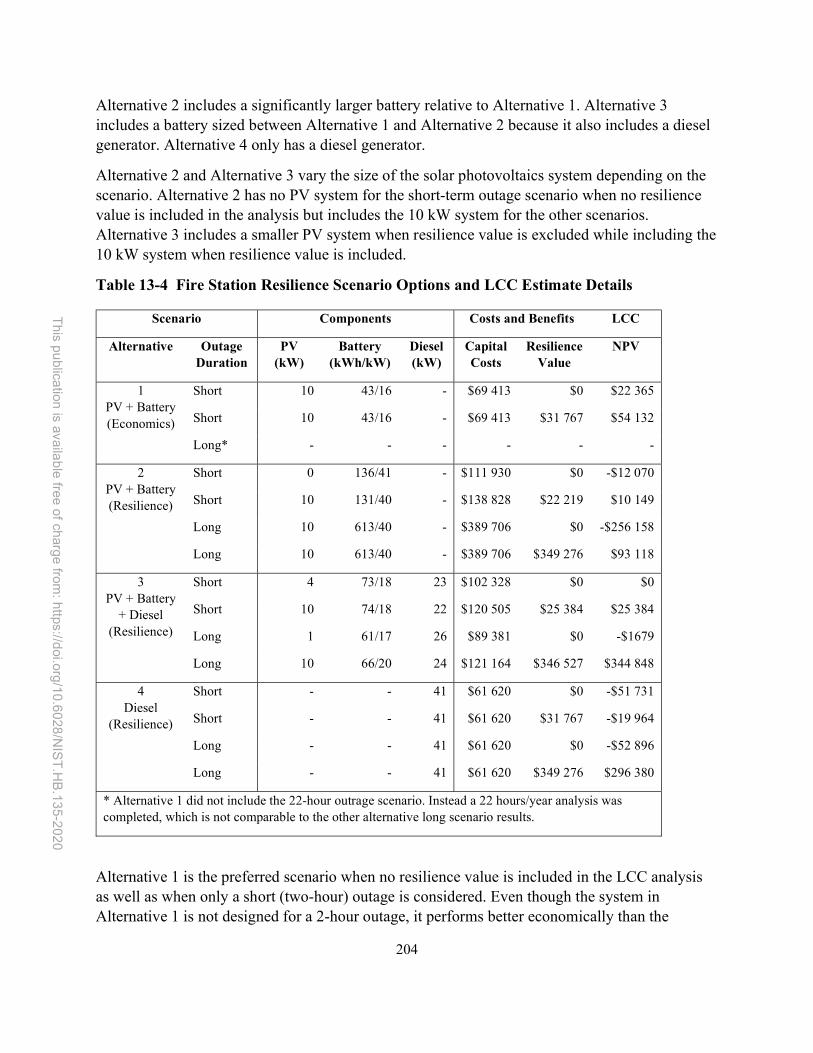
204

This p

ublica

tion is ava

ilab

le free

of ch

arge

from: h

ttps://doi.o

rg/1

0.6

028

/NIS

T.H

B.13

5-202

0

Alternative 2 includes a significantly larger battery relative to Alternative 1. Alternative 3 includes a battery sized between Alternative 1 and Alternative 2 because it also includes a diesel generator. Alternative 4 only has a diesel generator.

Alternative 2 and Alternative 3 vary the size of the solar photovoltaics system depending on the scenario. Alternative 2 has no PV system for the short-term outage scenario when no resilience value is included in the analysis but includes the 10 kW system for the other scenarios. Alternative 3 includes a smaller PV system when resilience value is excluded while including the 10 kW system when resilience value is included.

Table 13-4 Fire Station Resilience Scenario Options and LCC Estimate Details

Scenario Components Costs and Benefits LCC

Alternative Outage Duration

PV (kW)

Battery (kWh/kW)

Diesel (kW)

Capital Costs

Resilience Value

NPV

1 PV + Battery (Economics)

Short 10 43/16 - $69 413 $0 $22 365

Short 10 43/16 - $69 413 $31 767 $54 132

Long* - - - - - -

2 PV + Battery (Resilience)

Short 0 136/41 - $111 930 $0 -$12 070

Short 10 131/40 - $138 828 $22 219 $10 149

Long 10 613/40 - $389 706 $0 -$256 158

Long 10 613/40 - $389 706 $349 276 $93 118

3 PV + Battery

+ Diesel (Resilience)

Short 4 73/18 23 $102 328 $0 $0

Short 10 74/18 22 $120 505 $25 384 $25 384

Long 1 61/17 26 $89 381 $0 -$1679

Long 10 66/20 24 $121 164 $346 527 $344 848

4 Diesel

(Resilience)

Short - - 41 $61 620 $0 -$51 731

Short - - 41 $61 620 $31 767 -$19 964

Long - - 41 $61 620 $0 -$52 896

Long - - 41 $61 620 $349 276 $296 380

* Alternative 1 did not include the 22-hour outrage scenario. Instead a 22 hours/year analysis was completed, which is not comparable to the other alternative long scenario results.

Alternative 1 is the preferred scenario when no resilience value is included in the LCC analysis as well as when only a short (two-hour) outage is considered. Even though the system in Alternative 1 is not designed for a 2-hour outage, it performs better economically than the

205

This p

ublica

tion is ava

ilab

le free

of ch

arge

from: h

ttps://doi.o

rg/1

0.6

028

/NIS

T.H

B.13

5-202

0

alternatives designed to withstand the outage. Alternative 1 is not designed to handle the long outage and is, therefore, excluded from the long outage analysis. When comparing Alternative 2, 3, and 4, Alternative 3 is the preferred option regardless of the scenario because it leads to the greatest net savings (or lowest net costs), which is driven by the lower costs of diesel generators and operation than battery storage at the time of the study (2016). Note that these results may not hold in the future because of the trend i of decreasing battery storage costs.

Table 13-5 Fire Station Resilience Scenario LCC Summary

Scenario Short outage; no resilience value

Long outage; no resilience value

Short outage; resilience value

Long outage; resilience value

Alternative 1 $22 365 - $54 132 -

Alternative 2 -$12 070 -$256 158 $10 149 $93 118

Alternative 3 $0 -$1679 $25 384 $344 848

Alternative 4 -$51 713 -$19 964 -$52 896 $296 380

Although this case study assists in showing how the net savings change with different system sizes and technologies and the importance of including all direct and indirect benefits and costs (e.g., resilience value), the analysis does not allow for direct comparisons across the system options for each scenario because the expected likelihoods of those scenarios occurring has not been introduced.

The alternatives and scenarios in this case study demonstrate the narrowing down of alternatives that should be considered in a final analysis. Alternative 1 is always preferred to the no-system baseline and, therefore, should represent the new baseline alternative to use for a more complete analysis. Additionally, Alternative 3 is always preferred to Alternatives 2 and 4, which deems one of the systems considered in Alternative 3 to be a potentially better option than Alternative 1. The analysis should be rerun in REopt to include the two systems in Alternative 3 designed with the resilience value included since these are aimed at different scenarios. The expected value for each system under each scenario should be estimated to allow for a probabilistic analysis. The decision on which system to install should be based on the combination of these estimates with the expected probability of these events occurring over the study period to determine which alternative has the greatest expected net savings.

13.2.2 Example: Energy Resilience Project using the Energy Resilience Assessment (ERA) Tool

The example provided below is based on information available in Judson et al. (2016), Savena et al. (2017), and Castillo (2017). The ERA tool has been designed using information gathered from four site visits to installations in combination with location-specific data from IEEE (2007). ERA provides an analysis of over 40 energy system architectures to evaluate the life-cycle cost

206

This p

ublica

tion is ava

ilab

le free

of ch

arge

from: h

ttps://doi.o

rg/1

0.6

028

/NIS

T.H

B.13

5-202

0

and resilience performance for mission-critical operations. The architectures are a combination of the following components:

Grid-tied solar photovoltaics “Island-able” solar photovoltaic Building generator Central generator Uninterruptible power supply (UPS) 1-day load battery Microgrid Cogeneration Fuel cell Grid electricity Local load

For additional information on ERA, see Section 16.3.3.

The results for the example in Savena et al. (2017) are shown in Figure 13-3 and Figure 13-4. For this example, assume that the minimum level of resilience is that provided by the status quo system (baseline alternative). Given the available cost data and resources, ERA simulates the different architectures using historically based disruptions and generates both LCC and unserved energy loads (demand that cannot be supplied due to disruption in supply). Figure 13-3 shows the levelized LCC ($/kWh) and unserved energy (MWh) over a 10-year study period. The baseline case is Scenario 2, using utility-provided electricity and existing generators. An alternative scenario is preferred to the baseline if both the LCC and unserved energy are lower, which, based on these criteria, are the six scenarios (Scenarios 19, 24, 7, 9, 22 and 20) to the right of the baseline (Scenario 2).

These remaining scenarios can now be compared to determine which is the preferred scenario given the relative importance of each criteria in the analysis. If the goal of the project is to improve resilience by the greatest amount without increasing LCC, then Scenario 9 (microgrid, central generators, and island-able solar) is preferred because it leads to the lowest unserved energy load at lower LCC than the baseline. Note that Scenario 9 is preferred to Scenario 24 (microgrid, central and building generators, and island-able solar because it leads to the same unserved energy load but has lower LCC. If the goal is to at least maintain the current level of resilience while lowering LCC, then Scenario 20 is optimal because it leads to the lowest LCC at the same level of resilience as the baseline. If a relatively equal weight is placed on both cost and resilience, it’s feasible that the optimal design would be Scenario 22 (central and building generators, UPS, and grid-tied solar), which leads to a slightly higher LCC than Scenario 20 while lowering the unserved energy significantly.

207

This p

ublica

tion is ava

ilab

le free

of ch

arge

from: h

ttps://doi.o

rg/1

0.6

028

/NIS

T.H

B.13

5-202

0

Figure 13-3 LCC versus Unserved Energy (Historical Outage Rates) (Castillo, 2017)

Focusing solely on historical disruption data may miss low probability, high-impact events that may occur, particularly as security concerns increase and severe weather events become more frequent. Instead of using only historical data to randomize disruptions, Figure 13-4 shows total LCC ($ million) and unserved energy load (MWh) results over a 10-year study period assuming the occurrence of a two-week power outage (referred to as a “black sky” event). Such an extreme event shows the vulnerability of the facility to long disruptions, with unserved energy rising from under 60 MWh for the baseline scenario to nearly 200 MWh. Based on these results, eight scenarios have lower LCC and the same or better resilience than the baseline. Of those eight, Scenario 24 has the lowest LCC, with relatively low unserved energy loads (Scenario 9 has the same resilience but slightly higher LCC). Under a goal of reaching the lowest unserved energy load while not increasing LCC, Scenario 26 would be the best choice because it leads to the highest level of resilience. Note that Scenario 11 also reaches the same resilience level, but at slightly higher costs. Depending on the prioritization of economics and resilience and the concern for extreme events, the optimal design may change.

208

This p

ublica

tion is ava

ilab

le free

of ch

arge

from: h

ttps://doi.o

rg/1

0.6

028

/NIS

T.H

B.13

5-202

0

Figure 13-4 LCC versus Unserved Energy (2-Week Outage) (Castillo, 2017)

Note that each resilience project is unique, and the results of this example should not be used as recommendations for a decision on a specific project. A separate analysis should be completed to determine the feasible and optimal energy system designs.

This example has focused on the trade-off between two criteria, economics (i.e., LCC) and resilience (i.e., unserved energy). However, the criteria to be included and the relative importance of each criterion could be broader. For example, the facility may have multiple goals: improve energy resilience, increase energy and water conservation, and lower LCC. Unless the additional goals can be defined as minimum requirements (in which case it is an additional constraint), all goals will have to be optimized simultaneously based on the analyst’s defined preferences and priorities (which might derive from a government or agency directive).

The example also includes a single resilience metric for the entire facility. Multiple metrics within each criterion may be needed to determine the impact on the facility. For example, resilience can be measured by numerous metrics that may require trade-offs, such as SAIDI (average outage duration), SAIFI (average number of interruptions), and availability (percent of time operational). Depending on the facility, the length of an outage may be much more important than the number of outages or vice versa. Providing several metrics of resilience can provide a more complete representation of the facility’s performance.

Even a single metric, such as unserved energy, may need to be disaggregated, such as by timing of the disruption or which functions are impacted. A disruption during a peak day, week, or

209

This p

ublica

tion is ava

ilab

le free

of ch

arge

from: h

ttps://doi.o

rg/1

0.6

028

/NIS

T.H

B.13

5-202

0

month in which mission-critical activities are taking place at the facility could be of greater importance than during non-peak times. A disruption to a building used for mission-critical activities is of greater importance than that to a building used for mission- independent activities. A Mission Dependency Index (MDI), developed to capture the relative criticality of infrastructure assets with respect to organizational missions may be needed to prioritize the energy outages based on time and place, depending on the functions affected.

The level of complexity of the analysis is determined by the number of objectives or goals, criteria for evaluation, and the level of detail required in quantifying the metrics for each criterion.

210

This p

ublica

tion is ava

ilab

le free

of ch

arge

from: h

ttps://doi.o

rg/1

0.6

028

/NIS

T.H

B.13

5-202

0

14 Evaluating the Impact of Deferred Maintenance

Deferred maintenance has been defined as “maintenance that was not performed when it should have been or was scheduled to be and which, therefore, is put off or delayed for a future period” (NRC, 2001). Federal agencies regularly postpone recommended maintenance for building components to reduce operational budgets. This short-sighted approach can lead to lower equipment performance and more frequent failure rates that increase the number and magnitude of repairs and replacements of the equipment. Figure 14-1 is a visual representation of the potential impact of deferred maintenance on the performance (condition) of equipment with and without normal maintenance. As the time in service increases, the likelihood of deferred maintenance accelerating the deterioration of the equipment increases, leading to a shorter service life. Note that this example differs from the assumed linear deterioration of equipment in the example in Section 4.5.3.

Figure 14-1 Impact of Maintenance on Equipment Condition (Replicated from NRC

(2012))

14.1 Deferred Maintenance in the Federal Government

GAO has consistency identified poorly maintained buildings as a risk to the federal government. In 2003, GAO designated federal real property as a “high-risk” area in part due to deteriorating facilities (GAO, 2003). In 2009, GAO stated that “agencies continue to retain excess property and face challenges from repair and maintenance backlogs” (GAO, 2009a). The backlog

211

This p

ublica

tion is ava

ilab

le free

of ch

arge

from: h

ttps://doi.o

rg/1

0.6

028

/NIS

T.H

B.13

5-202

0

amounted to tens of billions of dollars in 2007 across six agencies32 and “may have a significant effect on future budget resources and our nation’s long-term fiscal sustainability” (GAO, 2008).33 GAO provided recommendations for agencies to implement to adequately identify, document, and quantify deferred maintenance and repair backlogs as well as for reporting annual funding to address the backlog and the resulting outcome of those expenditures.

With this issue in mind, the Federal Facilities Council (FFC) asked the National Academy of Sciences’ (NAS) National Research Council (NRC) to appoint an ad hoc committee to develop methods, strategies, and procedures to predict outcomes of investments in maintenance and repair of federal facilities. The resulting report, published in 2012, is titled “Predicting Outcomes of Investments in Maintenance and Repair of Federal Facilities,” and provided findings and recommendations to address the issue of deferred maintenance and repair (NRC, 2012). Those relevant to this handbook are highlighted below.34

First, timely investments in facilities M&R can lead to an array of beneficial outcomes. Table 14-1 replicates Table S.1 from NRC (2012) listing these benefits, which range across five outcome categories: mission-related, compliance-related, condition-related, efficient operations, and stakeholder-driven outcomes. Measures for each outcome are provided, many of which are discussed elsewhere in this handbook. A few additional metrics to highlight include building/facility functionality index and cost per person (mission-related), building/facility condition index (condition-related), and number and cost of worker compensation claims (compliance-related).

Second, deteriorating facilities and systems pose risks to the federal government and the public that vary from facility to facility and, therefore, the appropriate strategies, practices, and methods to implement will also vary by facility and/or agency. Federal agencies should implement strategic approaches for investing in facilities maintenance and repair to achieve the best combination of beneficial outcomes and mitigated risks.

Third, agencies should prioritize investments using a risk-based process and establish standard data collection and updating methods to evaluate progress, making reliable and appropriate data and information essential in evaluating investments and reporting outcomes from those investments.

Fourth, agencies should implement best practices from the private sector to manage and mitigate the risks and provide transparency to decision makers on the outcomes of, and risks posed by, investments in maintenance and repair projects and activities.

32 The reported values were deemed incomparable due to differences in how deferred maintenance was reported. 33 Federal real property remained listed as a “high risk” issue in 2019 (GAO, 2019) 34 In total there were nine findings and seven recommendations. See NRC (2012) for more details.

212

This p

ublica

tion is ava

ilab

le free

of ch

arge

from: h

ttps://doi.o

rg/1

0.6

028

/NIS

T.H

B.13

5-202

0

Table 14-1 Benefits from Maintenance and Repair Investments

Outcomes

Mission-Related Compliance-Related Condition-Related Efficient Operations

Stakeholder-Driven

Improved Reliability

Fewer Accidents & Injuries

Improved condition

Less reactive, unplanned M&R

Customer satisfaction

Improved Productivity

Fewer building-related illnesses

Reduced backlog of deferred M&R

Lower operating costs

Improved public image

Functionality Fewer insurance claims, lawsuits, &

regulatory violations

Lower LCC

Efficient Space Utilization

Cost avoidance

Reduced resource use

Reduced GHG emissions

Increasingly during the 2010s, agencies began to identify and quantify their deferred maintenance and repair backlog, but minimal progress has been made on reducing that backlog. GAO (2014) reviewed progress since its 2009 report and found that agencies are typically following eight of nine leading practices, with the only practice not well implemented being that of identifying funding allotted to managing the backlog. However, GAO’s Federal Real Property Profile (FRPP) estimated the backlog in fiscal year 2012 for the five agencies reviewed by GAO as ranging from $0.9 billion to $14.4 billion and totaling $37.8 billion. If left unchecked, these backlogs “can result in more expensive repairs, higher operating costs, and diminishing performance of the facilities” GAO (2014).

There are opportunities to concurrently address these backlogs in deferred maintenance and repairs along with energy and water conservation measures (ECMs). Depending on the facility, the potential for reducing the backlog will vary depending on the potential ECMs and their overlap with the deferred maintenance and repairs. For example, two projects that were both funded by the American Recovery and Reinvestment Act of 2009 led to very different outcomes related to deferred maintenance. The renovation of the Forrestal Building in Washington, D.C cost $28.1 million and reduced that facility’s backlog by merely $134 000 while the renovation of the Martinsburg Medical Center in Martinsburg, WV cost $5.5 million and reduced its backlog by $4.8 million (GAO, 2014). The reduced backlog was much higher for Martinsburg because the selected ECMs were associated with the equipment that had substantial deferred maintenance while the ECMs for the Forrestal Building were not.

Deferred maintenance can be incorporated into economic analysis in several ways. The most common is to incorporate the impacts of deferred maintenance (e.g., equipment deterioration)

213

This p

ublica

tion is ava

ilab

le free

of ch

arge

from: h

ttps://doi.o

rg/1

0.6

028

/NIS

T.H

B.13

5-202

0

into the baseline alternative estimates, including higher O&M costs and more frequent and costly repair and replacement costs. Along with the direct costs associated with the deferred maintenance, the indirect benefits and costs can be included by incorporating metrics measuring the outcomes listed in Table 14-1. Another way is for a reduction in deferred maintenance to be included in a project as a minimum requirement (e.g., reduce the current backlog by at least $100 000 for every $1 million spent on a resource conservation project). By incorporating deferred maintenance as a constraint, it will ensure there is a reduction in the existing backlog.

It is important to ensure that the analyst does not double-count the benefits and costs related to reductions in the backlog of deferred maintenance. A reduction in one dollar of deferred maintenance on an air conditioner due to replacement does not necessarily translate directly to one dollar saved in the LCCA. Incorporating the implications of the deferred maintenance into the baseline case ensures that the (direct and indirect) outcomes from the deferred maintenance are incorporated only once.

The authors were unable to find a realistic case study that evaluates the implications of deferred maintenance in terms of the rate of deterioration of equipment. Therefore, a simplified hypothetical example is provided to assist the reader in understanding why and how deferred maintenance should be evaluated.

14.2 Example: Deferred Maintenance

Assume that a facility manager is trying to determine whether to replace an existing cooling unit with a new, more efficient unit. The baseline system is ten years old and has 25-year service life with regular maintenance. The minimal acceptable condition entails the unit consuming 115 % of its rated performance. The system is assumed to deteriorate at 1% annually starting in year 11 of operation when regularly scheduled maintenance is performed according to the manufacturer’s specifications. The system deteriorates at an accelerated 3% annually starting in year 11 of operation when maintenance is deferred, which decreases the expected service life to 16 years. Figure 14-2 shows the operating condition of the 10-year old baseline system with regular and deferred maintenance for the selected 25-year study period. Note that after each replacement, the condition of the equipment is optimal because it is new. Therefore, there are years in which the system with deferred maintenance performs better than the system with regular maintenance, but at the cost of more frequent replacements.

214

This p

ublica

tion is ava

ilab

le free

of ch

arge

from: h

ttps://doi.o

rg/1

0.6

028

/NIS

T.H

B.13

5-202

0

Figure 14-2 Impact of Maintenance on Example Cooling Unit Condition

Assume that the alternative system being considered is identical in terms of service and relative performance in relation to maintenance. The difference is that it reduces energy consumption by 40% when both units are operating optimally. Table 14-2 shows the energy consumption by the cooling unit for the 25-year study period (based on the service life of the alternative system with regular maintenance) for both the baseline and alternative systems with and without regular maintenance.

0.80

0.85

0.90

0.95

1.00

1.05

1 2 3 4 5 6 7 8 9 10 11 12 13 14 15 16 17 18 19 20 21 22 23 24 25

Con

diti

on o

f E

quip

men

t

Year

Deferred versus Regular Maintenance

Energy Consumption - Deferred Maint. Energy Consumption - Regular Maint.

215

This p

ublica

tion is ava

ilab

le free

of ch

arge

from: h

ttps://doi.o

rg/1

0.6

028

/NIS

T.H

B.13

5-202

0

Table 14-2 Energy Consumption (kWh) by Alternative and Maintenance

Baseline Alternative

Year Deferred Regular Deferred Regular

1 100 000 100 000 60 000 60 000

2 103 000 101 000 60 000 60 000

3 106 090 102 010 60 000 60 000

4 109 273 103 030 60 000 60 000

5 112 551 104 060 60 000 60 000

6 115 927 105 101 60 000 60 000

7 100 000 106 152 60 000 60 000

8 100 000 107 214 60 000 60 000

9 100 000 108 286 60 000 60 000

10 100 000 109 369 60 000 60 000

11 100 000 110 462 61 800 60 600

12 100 000 111 567 63 654 61 206

13 100 000 112 683 65 564 61 818

14 100 000 113 809 67 531 62 436

15 100 000 114 947 69 556 63 061

16 100 000 100 000 71 643 63 691

17 103 000 100 000 60 000 64 328

18 106 090 100 000 60 000 64 971

19 109 273 100 000 60 000 65 621

20 112 551 100 000 60 000 66 277

21 115 927 100 000 60 000 66 940

22 100 000 100 000 60 000 67 610

23 100 000 100 000 60 000 68 286

24 100 000 100 000 60 000 68 968

25 100 000 100 000 60 000 69 658 Note: Bold indicates that replacement threshold (115%) has been reached.

The baseline system is replaced at the end of year 6 and year 21 if maintenance is deferred and year 15 if maintenance is completed annually. The alternative system is replaced in year 16 if maintenance is deferred and year 25 if maintenance is completed annually.

For completing the LCCA, assume the following:

Cost of energy is $0.10/kWh

Baseline replacement cost is $10 000

Baseline maintenance cost is $100 annually

Alternative initial installation or replacement is $20 000

216

This p

ublica

tion is ava

ilab

le free

of ch

arge

from: h

ttps://doi.o

rg/1

0.6

028

/NIS

T.H

B.13

5-202

0

Alternative maintenance cost is $200 annually

Residual value is calculated using a linear depreciation

Discount rate is 3 %

The resulting NPV cash flows, LCC, and NS are provided in Table 14-3. The baseline system with deferred maintenance leads to higher LCC than when regular maintenance is completed. The alternative system leads to NS relative to the baseline system regardless of the maintenance decisions. However, implementing regular maintenance for the alternative system leads to the highest NS.

Table 14-3 NPV Cash Flow, LCC, and NS by Alternative and Maintenance

Baseline Alternative

Year Deferred Regular Deferred Regular

1 9709 9806 25 243 25 243

2 9709 9614 5656 5844

3 9709 9427 5491 5674

4 9709 9243 5331 5509

5 9709 9063 5176 5348

6 18 084 8886 5025 5192

7 8131 8712 4879 5041

8 7894 8542 4736 4894

9 7664 8376 4599 4752

10 7441 8212 4465 4613

11 7224 8052 4465 4522

12 7014 7895 4465 4433

13 6810 7741 4465 4346

14 6611 7590 4465 4260

15 6419 13 797 4465 4176

16 6232 6294 16 928 4094

17 6232 6111 3630 4013

18 6232 5933 3524 3934

19 6232 5760 3422 3856

20 6232 5592 3322 3780

21 11 607 5429 3225 3706

22 5219 5271 3131 3633

23 5067 5118 3040 3561

24 4919 4969 2952 3491

25 2985 3439 1821 3422

LCC $192 790 $188 872 $137 917 $131 339

NS ($3919) - $50 955 $57 533 Note: Bold indicates that replacement threshold (115%) has been reached.

217

This p

ublica

tion is ava

ilab

le free

of ch

arge

from: h

ttps://doi.o

rg/1

0.6

028

/NIS

T.H

B.13

5-202

0

Note that the use of an ESPC contract could also be implemented to create certainty on the investment costs and energy savings. FEMP provides guidance on determining and verifying O&M savings in ESPCs (FEMP, 2018).

14.3 Maintenance Programs

One of the most cost-effective ways to reduce the life-cycle cost of a building is through proper maintenance, but it requires appropriate resource allocation and planning. Chapter 5 of Sullivan, Pugh, Melendez, and Hunt (2010) distinguish key types of maintenance programs. Maintenance programs can be reactive (actions to repair equipment that is no longer operating correctly) or proactive (actions to maintain proper operation). The remainder of this section summarizes each type of maintenance program highlighted in Sullivan et al. (2010).

The most common approach is reactive maintenance (> 55 % of all facilities), which occurs only when obvious problems with equipment are identified due to a failure of the equipment to operate at minimal levels of performance. Deferring maintenance that could keep equipment operating at proper performance levels is part of a reactive maintenance approach, which decreases operational costs (both labor and materials) in the short term but is likely to increase unplanned equipment downtime and associated repair and replacement costs over the lifetime of the facility.

Proactive maintenance programs can be categorized as preventive, predictive, or reliability-centered. Preventive maintenance is the second most common approach (31 % of all facilities, according to the authors) and sets a maintenance schedule using predetermined time intervals. The set schedules help identify damaged equipment before obvious, potentially large, problems occur, which is particularly beneficial for equipment that is operated intermittently and/or by personnel who do not have enough knowledge, skills, and time to perform the preventive maintenance work.

Predictive maintenance sets schedules for maintenance activities when mechanical or operational conditions reach pre-defined “unacceptable” levels using fault detection through monitoring equipment, allowing for repairs or replacements that prevent a more costly failure in the future. This approach is not common (12 % of all facilities) because it requires more extensive planning and funding. It is most effective if the equipment conditions can be monitored and facility personnel have adequate knowledge, skills, and time to perform the predictive maintenance work. The ability to more accurately predict maintenance requirements provides more lead time to plan for the necessary labor and materials for repairs, allowing for more efficiency in operational budgets.

Reliability-centered maintenance combines proactive maintenance techniques with root cause failure analysis, and focuses on the potential solutions to minimize or eliminate the same failure in the future. Such an approach uses a more integrated design approach to include equipment re-design or modification as options to minimize or eliminate problems. The approach will

218

This p

ublica

tion is ava

ilab

le free

of ch

arge

from: h

ttps://doi.o

rg/1

0.6

028

/NIS

T.H

B.13

5-202

0

prioritize the performance of expensive and important equipment while deferring maintenance on inexpensive or less important equipment. This approach is most effective when facilities personnel have the knowledge, skills, and time to perform all required activities, not just a specific maintenance task.

Of the top performing facilities that use the reliability-centered maintenance approach, 45 % to 55 % primarily implement predictive approaches, 25 % to 35 % primarily implement preventive maintenance approaches, and < 10 % primarily implement reactive maintenance approaches. This implies that the appropriate maintenance program to maximize resilience varies based on the specific needs of a facility. For more details on predictive maintenance technologies and how to design a reliability-centered maintenance program, see Sullivan et al. (2010).

The remainder of this section will provide examples of maintenance programs based on case studies provided in Sullivan et al. (2010).

14.4 Example: Predictive Maintenance of a Facility

This section uses multiple examples provided in Sullivan et al. (2010), and combines them into a single facility example. Note that these examples are not a real case study and have been altered from the original information. The facility has a combination of preventive and reactive maintenance activities, but the facility managers expect that implementing predictive maintenance approaches could reduce O&M costs and improve the reliability of the building’s systems.

One of the top issues identified was the condition of the roof, for which maintenance has been deferred for many years. Assume the facility has a 360 000 ft2 roof that is 22 years old (expected life of 40 years if properly maintained) and experiencing several leaks. A visual inspection of the roof fails to identify where the leaks are occurring. Continuing to defer maintenance on the roof (excluding patching the leaks) is expected to lead to a complete failure of the roof membrane in five years. Cost estimates to replace the roof range between $2.5 and $3 million. For simplicity, assume the lower end of this range and exclude the financial damages of the leaks.

An alternative to replacing the entire roof is to use predictive methods to identify areas of the roof that are expected to be causing leaks or may leak in the future. An initial infrared (IR) inspection identified 1200 ft2 of roof required replacement at a cost of $20 700. The following year another IR inspection was performed that found 1400 ft2 of roof requiring replacement at a cost of $18 200. A roof IR inspection program was implemented with an annual roof survey, resulting in less than 200 ft2 of roof replacement in any one of the following four years with a low of 30 ft2 as shown in Table 14-4. The total cost for roof repair using IR to predict which roof area will lead to a leak for the six years considered was less than $60 000.

219

This p

ublica

tion is ava

ilab

le free

of ch

arge

from: h

ttps://doi.o

rg/1

0.6

028

/NIS

T.H

B.13

5-202

0

Table 14-4 Costs of Maintenance Approach

Deferred Maintenance Predictive Maintenance

Year Cost Area Replaced

(ft2)

SPV NPV Year Cost Area Replaced

(ft2)

SPV NPV

0 - 1.000 - 0 $20 705 1208 1.000 $20 705

1 - 0.971 - 1 $18 217 1399 0.971 $17 689

2 - 0.943 - 2 $5900 195 0.943 $5564

3 0.915 - 3 $1000 30 0.915 $915

4 - 0.888 - 4 $4850 190 0.888 $4307

5 $2 500 000 360 000 0.863 $2 157 500 5 $4900 180 0.863 $4229

Total 360 000 $2 157 500 Total 3202 $53 408

Assume that the facility is also considering implementing a predictive HVAC maintenance program instead of the current preventive and reactive maintenance activities, if the predictive program is deemed cost-effective. This includes using available predictive tools to find cost savings for three identified potential areas of improvement.

First, the facility is considering switching from a preventive maintenance approach of maintaining two centrifugal compressors using a time-based methodology to a condition-based (predictive) method that regularly completes an oil analysis to identify water contamination and particle counts. By scheduling repairs only when the presence of contamination or high ferrous and non-ferrous particle counts are identified, the facility can reduce maintenance and lost productivity costs by $55 000 annually. Even if the equipment is tested daily at a cost of $100/sample ($36 500 annually), the predictive maintenance approach is preferred.

Second, the facility’s two air compressors were operating excessively given their expected loads, and plant management assumed a third compressor was needed, at a cost of $50 000. Instead, the facility invested $1000 on an ultrasound inspection of its air system. The ultrasound technician detected 64 air leaks accounting for an estimated total air loss of 295 CFM (26% of total system capacity). The cost to operate the two air compressors is approximately $50 000 annually (calculated at $0.04/kWh) at a total of 1120 CFM. Eliminating the air leaks would save $13 000 annually. The cost of sealing all the identified air leaks would cost $20 000, leading to a SPB of less than 2 years.

Third, the facility managers want to ensure the compressors are operating properly. A data logger is installed to measure operation at five-minute intervals, which shows that the compressors are cycling excessively at 6.5 on/off cycles per hour versus the expected 2.0 or fewer. The current compressors are determined to be oversized for the current loads. An analysis should be

220

This p

ublica

tion is ava

ilab

le free

of ch

arge

from: h

ttps://doi.o

rg/1

0.6

028

/NIS

T.H

B.13

5-202

0

completed to determine if it would be optimal to keep operating both compressors, replace them with smaller, correctly-sized models, or operate using only one compressor based on the facility’s operational constraints.

Many predictive maintenance technologies like those highlighted above are available to improve operational performance of a facility and can be included in projects covered by this handbook to make the economic case for improved efficiency. Although the examples presented are somewhat simplified, they provide good examples of how implementing smarter maintenance programs can significantly reduce overall facility costs.

221

This p

ublica

tion is ava

ilab

le free

of ch

arge

from: h

ttps://doi.o

rg/1

0.6

028

/NIS

T.H

B.13

5-202

0

222

This p

ublica

tion is ava

ilab

le free

of ch

arge

from: h

ttps://doi.o

rg/1

0.6

028

/NIS

T.H

B.13

5-202

0

15 Cross-Cutting Goals

Numerous cross-cutting goals are identified in EO 13834: acquisition, electronics stewardship, data center management, and GHG management and reporting. Although LCCA cannot be the only approach considered in meeting these goals, it plays an important role in identifying the most cost-effective. The example included below is for data center efficiency because it is the most directly related to facility performance.

15.1 Example: Data Center

At the end of FY 2014, DOE’s BTO started the Data Center Better Buildings Challenge, an offshoot of the Better Buildings Challenge.35 The program requested that participating data centers commit to a 20 % energy efficiency improvement in the non-information technology (I.T.) portions of their data centers. DOE’s focus was not so much the electronic components of a data center, but instead the power distribution and cooling/humidity control systems in the facilities. However, data centers also consume significant amounts of energy in the electronic processing itself.

EO 13834 states that agencies should “implement practices that promote energy-efficient management of servers and federal data centers.” FEMP offers guidance on energy efficiency in data centers (FEMP, 2011a), including data center metrics and benchmarking values, as shown in Table 15-1. The emphasis is placed on the supporting equipment within a data center, using key metrics such as power usage effectiveness (PUE), the total energy used by a data center divided by the portion of that energy strictly devoted to the computing operations, and energy reuse effectiveness (ERE), the ratio of the total energy to run the data center facility minus the reuse energy (energy that gets productively used elsewhere, within or outside of the facility) to the total energy drawn by all IT equipment. Another metric, rack cooling index (RCI), measures how effectively I.T. equipment is cooled relative to the equipment’s intake temperature guidelines. Airflow efficiency is a measure of how efficiently air is moved through the data center, from the supply to the return. Cooling system efficiency (e.g., kW/ton for chiller-driven cooling or EER for direct expansion computer room A.C., or CRAC, units) is a measure of the efficiency of the HVAC system. Any combination of these metrics – and potentially even others – could be deemed appropriate depending on the specific data center being evaluated. See FEMP (2011a) for additional information on these metrics.

35 The Data Center Better Buildings Challenge (portfolio reduction of 20% in infrastructure intensity in 10 years) as well as the Data Center Accelerator program (25 % reduction in a facility over five years for a single facility) are no longer actively accepting partners and have sunset as of the end of 2019. However, it is expected that a similar program will exist in some form in the future, and therefore, the example provided in this chapter may remain applicable.

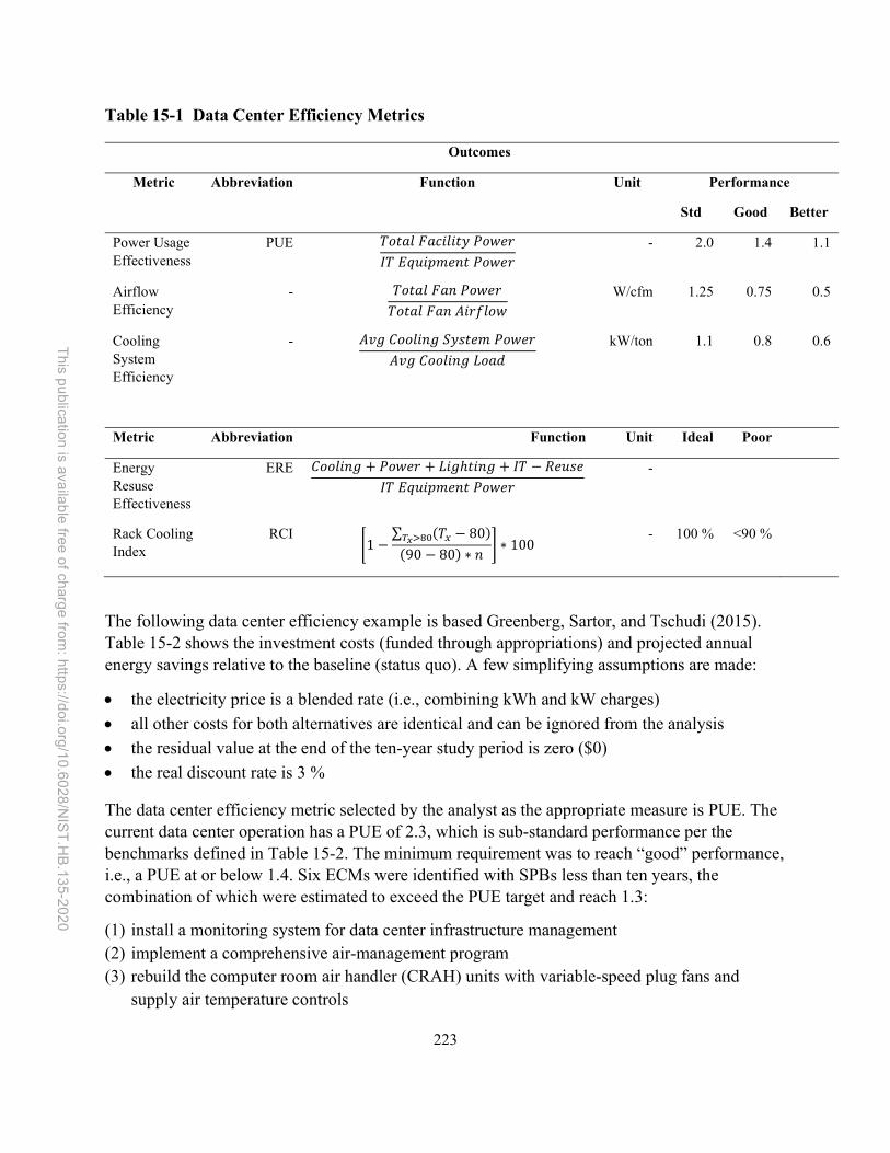
223

This p

ublica

tion is ava

ilab

le free

of ch

arge

from: h

ttps://doi.o

rg/1

0.6

028

/NIS

T.H

B.13

5-202

0

Table 15-1 Data Center Efficiency Metrics

Outcomes

Metric Abbreviation Function Unit Performance

Std Good Better

Power Usage Effectiveness

PUE 𝑇𝑜𝑡𝑎𝑙 𝐹𝑎𝑐𝑖𝑙𝑖𝑡𝑦 𝑃𝑜𝑤𝑒𝑟

𝐼𝑇 𝐸𝑞𝑢𝑖𝑝𝑚𝑒𝑛𝑡 𝑃𝑜𝑤𝑒𝑟

- 2.0 1.4 1.1

Airflow Efficiency

- 𝑇𝑜𝑡𝑎𝑙 𝐹𝑎𝑛 𝑃𝑜𝑤𝑒𝑟

𝑇𝑜𝑡𝑎𝑙 𝐹𝑎𝑛 𝐴𝑖𝑟𝑓𝑙𝑜𝑤

W/cfm 1.25 0.75 0.5

Cooling System Efficiency

- 𝐴𝑣𝑔 𝐶𝑜𝑜𝑙𝑖𝑛𝑔 𝑆𝑦𝑠𝑡𝑒𝑚 𝑃𝑜𝑤𝑒𝑟

𝐴𝑣𝑔 𝐶𝑜𝑜𝑙𝑖𝑛𝑔 𝐿𝑜𝑎𝑑

kW/ton 1.1 0.8 0.6

Metric Abbreviation Function Unit Ideal Poor

Energy Resuse Effectiveness

ERE 𝐶𝑜𝑜𝑙𝑖𝑛𝑔 + 𝑃𝑜𝑤𝑒𝑟 + 𝐿𝑖𝑔ℎ𝑡𝑖𝑛𝑔 + 𝐼𝑇 − 𝑅𝑒𝑢𝑠𝑒

𝐼𝑇 𝐸𝑞𝑢𝑖𝑝𝑚𝑒𝑛𝑡 𝑃𝑜𝑤𝑒𝑟

-

Rack Cooling Index

RCI 1 −

∑ (𝑇 − 80)

(90 − 80) ∗ 𝑛∗ 100

- 100 % <90 %

The following data center efficiency example is based Greenberg, Sartor, and Tschudi (2015). Table 15-2 shows the investment costs (funded through appropriations) and projected annual energy savings relative to the baseline (status quo). A few simplifying assumptions are made:

the electricity price is a blended rate (i.e., combining kWh and kW charges)

all other costs for both alternatives are identical and can be ignored from the analysis

the residual value at the end of the ten-year study period is zero ($0)

the real discount rate is 3 %

The data center efficiency metric selected by the analyst as the appropriate measure is PUE. The current data center operation has a PUE of 2.3, which is sub-standard performance per the benchmarks defined in Table 15-2. The minimum requirement was to reach “good” performance, i.e., a PUE at or below 1.4. Six ECMs were identified with SPBs less than ten years, the combination of which were estimated to exceed the PUE target and reach 1.3:

(1) install a monitoring system for data center infrastructure management (2) implement a comprehensive air-management program (3) rebuild the computer room air handler (CRAH) units with variable-speed plug fans and

supply air temperature controls

224

This p

ublica

tion is ava

ilab

le free

of ch

arge

from: h

ttps://doi.o

rg/1

0.6

028

/NIS

T.H

B.13

5-202

0

(4) install a small, dedicated chiller for the print shop (5) re-commission the chiller plant, including implementing chilled and condenser water

temperature reset, and the addition of a water-side economizer (6) turn off unneeded uninterruptible power supply (UPS) modules and power distribution units

(PDUs), usually a transformer and breaker panel

Table 15-2 shows the benefits and costs of implementing the six ECMs. Note that ECM (2) and (3) as well as ECM (4) and (5) are combined within the following analysis. The installation costs total $1.05 million while the projected energy cost savings amount to $314 000, which leads to a SPB of under 4 years.

Table 15-2 Data Center ECMs and Costs

ECMs Installed Cost

Annual Energy

Savings

Annual Savings

SPB

($) (kWh) ($) (Yrs) 1 - Monitoring System 202 000 373 000 24 300 8.3 2 & 3 - Air-management program; Rebuild the CRAH units 761 000 3 829 000 250 000 3.0 4 & 5 - Install small chiller for print shop; Re-commission chiller plant

80 000 465 000 30 200 2.6

6 - Turn off unneeded UPS modules and PDUs 3000 144 000 9400 0.3 Total 1 046 000 4 832 000 314 000 3.3

Table 15-3 shows the annual cash flows and annual and cumulative present value net savings. Over the ten-year study period, the present value net savings is over $1.6 million. From an efficiency perspective, total average power decreases from 1386 kW to 811 kW. Of the total energy consumed by the data center, IT equipment increases in share from 44 % to 74 % due to the reduction in humidity control operation, as well as increased fan and HVAC equipment efficiency.

This simple example shows how LCCA can be applied for data center efficiency improvements.

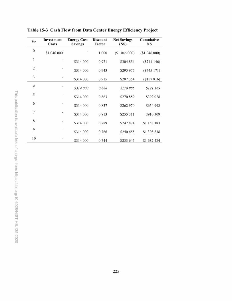
225

This p

ublica

tion is ava

ilab

le free

of ch

arge

from: h

ttps://doi.o

rg/1

0.6

028

/NIS

T.H

B.13

5-202

0

Table 15-3 Cash Flow from Data Center Energy Efficiency Project

Yr Investment

Costs Energy Cost

Savings Discount Factor

Net Savings (NS)

Cumulative NS

0

$1 046 000 -

1.000

($1 046 000)

($1 046 000)

1 -

$314 000

0.971

$304 854

($741 146)

2 -

$314 000

0.943

$295 975

($445 171)

3 -

$314 000

0.915

$287 354

($157 816)

4 -

$314 000

0.888

$278 985

$121 169

5 -

$314 000

0.863

$270 859

$392 028

6 -

$314 000

0.837

$262 970

$654 998

7 -

$314 000

0.813

$255 311

$910 309

8 -

$314 000

0.789

$247 874

$1 158 183

9 -

$314 000

0.766

$240 655

$1 398 838

10 -

$314 000

0.744

$233 645

$1 632 484

226

This p

ublica

tion is ava

ilab

le free

of ch

arge

from: h

ttps://doi.o

rg/1

0.6

028

/NIS

T.H

B.13

5-202

0

16 Software for LCCA of Facilities and Systems

NIST, under sponsorship from FEMP, offers the Building Life Cycle Cost (BLCC) software program to provide economic analysis of proposed investments in buildings and building systems intended to reduce long-term operating costs. BLCC is useful for evaluating costs and savings related to energy efficiency, water conservation, and renewable energy projects, and for selecting project alternatives with the lowest life-cycle cost. Comparative economic measures can be computed for any project alternative, including net savings, savings-to-investment ratio, adjusted internal rate of return, and payback period. BLCC is appropriate for federal, state, and local government and private sector use and is available to the public, along with this handbook and the Annual Supplement to Handbook 135, free of charge at FEMP’s website devoted to life-cycle costing for buildings (http://energy.gov/eere/femp/building-life-cycle-cost-programs). BLCC is updated annually to include the current FEMP and OMB discount rates and the most recent DOE projections of energy price escalation rates. The program version number now includes the year for which it is current, e.g., BLCC version 5.3-19 is intended for use in 2019.

Note that BLCC was not explicitly designed to handle all of the scope presented in this handbook. Although BLCC has the technical capability to introduce costs related to sustainability and resilience, the terminology, structure, and guidance within BLCC may not be intuitive to analysts completing such evaluations.

NIST also provides the Energy Escalation Rate Calculator (EERC), which calculates an average annual escalation rate based on EIA energy cost projections and general inflation forecasts of the President’s Council of Economic Advisers. The calculator is updated annually with the latest EIA energy price projections, which are also embedded in the BLCC programs and in the discount factor tables of the Annual Supplement to Handbook 135. EERC can also be accessed from FEMP’s life-cycle costing web site (http://energy.gov/eere/femp/building-life-cycle-cost-programs).

Note that some computer programs previously developed by NIST under sponsorship from FEMP are no longer supported, including QI (Quick Input), DISCOUNT, and ERATES.

This chapter will discuss BLCC and EERC and highlight other software that is either currently used or may be useful for federal LCCA.

16.1 BLCC

The NIST Building Life-Cycle Cost (BLCC) computer program provides comprehensive economic analysis of proposed capital investments that are expected to reduce long-term operating costs of buildings or building systems. Numerous alternative designs can be evaluated simultaneously to determine which has the lowest life-cycle cost. Comparative economic measures can be calculated for any design alternative relative to the designated base case. BLCC complies with ASTM building economics standards as well as the guidance in this handbook.

227

This p

ublica

tion is ava

ilab

le free

of ch

arge

from: h

ttps://doi.o

rg/1

0.6

028

/NIS

T.H

B.13

5-202

0

16.1.1 Project Type, Reports, and Analysis Summary

BLCC provides economic analysis for different types of project evaluations, referred to as modules:

Federal Analysis, Financed Project: This is the module to be used for an LCCA of energy savings performance contracts (ESPCs), utility energy services contracts (UESC) or other alternatively financed investments in energy or water conservation in the federal government. The criteria used as defaults in this module are applicable to all agencies in the federal government.

FEMP Analysis, Energy Project: The criteria used as defaults in this module follow FEMP’s life-cycle costing rules according to 10 CFR 436A as they apply to energy and water conservation and renewable energy projects funded by agencies from direct appropriations.

OMB Analysis, Non-Energy Project: This module supports analyses that are subject to the life-cycle costing guidelines of OMB Circular A-94 for the following types of projects: (a) cost-effectiveness, lease-purchase, internal government investment, and asset sales, and (b) public investment and regulatory analyses

MILCON Analysis, Energy Project: This module supports LCC analyses, according to 10 CFR 436A, of agency-funded energy and water and renewable energy projects for military construction in the Army, Navy, and Air Force.

MILCON Analysis, ERCIP Project: This module can be used for generating the "ERCIP Report" for MILCON projects funded by the DoD Energy Resilience and Conservation Investment Program to retrofit existing energy systems.

MILCON Analysis, Non-Energy Project: This module supports LCC analyses of new acquisition or construction projects, lease-purchase decisions, modification of existing facilities and similar projects, the purpose of which is not primarily to assess resource conservation.

BLCC is useful for evaluating energy conservation projects in buildings. For example, it can be used to determine the economically optimal level of insulation in an attic, select the most cost-effective heating and cooling system in a given building and location, or evaluate the cost-effectiveness of a solar heating system. Estimates of annual energy requirements for each alternative and appropriate cost data are required for the analysis. Annually updated projections of rates of increase in energy prices from the EIA, by fuel type, rate type, and region of the country are built into BLCC. BLCC also has the capability of evaluating water conservation projects with data entry screens for water usage and cost data.

Six different reports are generated by BLCC. Each can be displayed to the screen, sent to the printer, or saved for later use.

228

This p

ublica

tion is ava

ilab

le free

of ch

arge

from: h

ttps://doi.o

rg/1

0.6

028

/NIS

T.H

B.13

5-202

0

Reports by project alternative:

• input data file listing • summary of life-cycle cost analysis • detailed life-cycle cost analysis • yearly cash flow analysis

Reports comparing project alternatives:

• Identification of lowest life-cycle cost alternative • Comparative economic analysis of any two alternatives, including net savings • Savings-to-investment ratio, adjusted internal rate of return on investment, payback period,

annual energy savings (in physical units), and reductions in air pollution emissions

For OMB projects, following the guidelines of Circular A-94, select either

Cost-effectiveness, lease-purchase, internal government investment, and asset sales, or Public investment and regulatory analyses.

16.1.2 Discounting in BLCC

End-of-year or Mid-year Discounting

If end-of-year discounting is selected, all annually recurring costs (including energy and water costs) will be discounted to the base date from the end of the year in which they occur. If mid-year discounting is selected, all annually recurring costs (including energy and water) will be discounted to the base date from the middle of the year. End-of-year discounting is the default for all types of analyses except MILCON ones. MILCON analyses require mid-year discounting, and the designated MILCON modules use mid-year discounting as the default.

Constant- or Current-Dollar Analysis for Financed Projects

Projects financed through ESPCs or UESCs may be performed in either constant or current dollars. Current-dollar analysis is the default for financed projects in BLCC. The reason is that it may be useful to compare current-dollar energy cost savings or total operational cost savings with contract payments, which generally are escalated to reflect anticipated nominal dollar price increases. In current-dollar analysis, the discount rate and all price escalation rates need to be entered in nominal (including inflation) terms. The default inflation rate in BLCC5 is the average long-term inflation rate calculated annually for DOE/FEMP projects according to 10 CFR 436.

If the analysis of ESPC or UESC projects is performed in constant dollars, all annual cash flows will be reported in constant dollars as of the base year. Any annual cost that is expected not to increase at the rate of general inflation during the study period will have to be assigned a negative escalation rate. In constant-dollar analysis, the underlying assumption is that all dollar amounts increase at the same rate of general inflation and only differential rates of escalation are entered. For example, assume that the contract payment charged by an ESCO is a fixed annual

229

This p

ublica

tion is ava

ilab

le free

of ch

arge

from: h

ttps://doi.o

rg/1

0.6

028

/NIS

T.H

B.13

5-202

0

amount that does not increase at the rate of inflation from year to year. In this case, the negative of the inflation rate (i.e., a differential rate of increase) must be entered to make the present value of the contract payments consistent with the present values of the other cash flows. (See also Chapter 3).

Note: If you switch from constant-dollar to current-dollar analysis after having created a file, BLCC5 will automatically convert the discount rate and all rates of escalation to nominal rates with the same rate of inflation that is used to compute the nominal DOE/FEMP discount rate. Likewise, if you switch from current-dollar to constant-dollar analysis, BLCC5 will automatically convert the discount rate and all rates of escalation to real rates.

16.1.3 Contract-Related Costs in BLCC

Contract-related costs are usually relevant only for the analysis of financed projects. BLCC5 allows you to divide these costs into annually recurring and non- recurring costs. Contract costs are assigned at the alternative level, since they may not be attributable to individual ECMs.

If annually recurring contract costs either escalate at rates that are non-uniform from year to year or if escalation rates differ for parts of the contractor payment, separate escalation rates can be assigned to each of the contract cost components. For example, contract costs may vary at rates equal to expected non-linear energy price escalation rates (e.g., at a faster rate in the first several years of a contract and then slower in subsequent years) rather than at a constant annual rate. Alternatively, a portion of the contractor payments may escalate at energy price escalation rates, another at OM&R escalation rates, and a third may be fixed.

Note: If the analysis is performed in constant dollars, any contract payments that do not change from year to year at the rate of general inflation need to be adjusted by the negative of the escalation rate to maintain them as constant-dollar amounts. The underlying assumption in constant-dollar analyses is that all amounts escalate at the same rate.

Some contract-related costs not included in the total annual contract payment may be one-time costs, such as implementation costs or financing procurement costs. Once created, the names of these costs can be edited if further non-annually recurring costs need to be included in the analysis and in the BLCC5 reports.

BLCC5 allows the user to vary the pattern of occurrence of annual contract costs similarly to annually recurring energy and OM&R costs. The usage indices make it possible to assign annual contract costs to various time periods during the study period. For example, management and administrative costs may be included in the annual contract payment during the contract term but may be incurred directly by the agency during the post-contract period. An index of 0 for a contract term of ten years and an index of 100 for the remaining years in the study period mean that annual management and administrative costs are incurred by the agency after the end of the contract term, i.e., 0% during the contract term and 100% after the contract term ends.

230

This p

ublica

tion is ava

ilab

le free

of ch

arge

from: h

ttps://doi.o

rg/1

0.6

028

/NIS

T.H

B.13

5-202

0

16.1.4 Operational Energy Costs and Emissions in BLCC

Energy Costs Energy costs are entered for the entire alternative regardless of whether the alternative is evaluated as a single component or sub-divided into several components (e.g., energy conservation measures). Energy costs are assumed to be annually recurring costs starting with the service date and continuing throughout the service period.

Energy-related data include the rate schedule, location, price, demand charges, utility rebates, and energy price escalation rates. The escalation rates are defaulted to the DOE escalation rates (i.e., those from EERC, which are retrieved automatically for the specified region, rate, and fuel type), and can be edited by the user to reflect other sources (e.g., future rates published by a utility).

Note: If annual demand charge or annual utility incentive (e.g., rebates) need to be escalated differently from the energy costs, you can proceed as follows:

create a new "energy cost" set annual consumption to zero in the energy usage screen and price/unit in the energy

cost screen edit the DOE energy price escalation rates

Note: The duration of the energy usage index begins with the service date (since energy consumption calculations begin with the service date), while the duration for energy price escalation rates begin at the start of the study period (since all prices are entered in base-year dollars).

Energy-related Emissions BLCC5 calculates air pollution emissions associated with energy use in buildings and building systems, as well as those attributable to energy conservation measures. Annual and life-cycle estimates are provided for carbon dioxide (CO2), sulfur dioxide (SO2), and nitrous oxide (NOx). Emission factors are specified for six different end-use energy types: electricity, distillate and residual fuel oil, natural gas, liquid petroleum gas (LPG), and coal. Emission factors for electricity are specific to the location of the project (U.S. state or District of Columbia). The economic cost of these emissions is not estimated. The emissions estimates are reported in kilograms (kg) in the Detailed LCC Analysis Report and the Comparative Analysis Report.

BLCC5 chooses default emission factors for CO2 and SO2 for fossil fuels consumed at the building site. To determine the NOx emission factor, which depends on the type of combustion equipment in which the fuel is used, users can select the appropriate end-use equipment from a drop-down list. To calculate emission factors for coal, BLCC5 assumes the use of bituminous, sub-bituminous, and lignite coal in equal proportions.

231

This p

ublica

tion is ava

ilab

le free

of ch

arge

from: h

ttps://doi.o

rg/1

0.6

028

/NIS

T.H

B.13

5-202

0

16.1.5 Residual Value in BLCC

The residual value factor is the percent of the initial replacement cost in base-year dollars remaining at the end of the study period (or at the end of the expected life of the replacement, whichever is sooner). A negative rate can be entered if the residual value is a disposal cost. BLCC5 uses the average annual rate of increase specified for the replacement cost along with this factor to compute the actual residual value in dollars.

Note: If a user does not want to use linear depreciation to estimate the residual value, the residual value factor should be set to 0.0 % and a separate investment cost object should be created that includes a one-time (negative) cost at the end of the study period.

Note: Non-capital replacement costs for MILCON analyses must be entered as non-annually recurring routine OM&R costs.

Note: Residual values are not included in the ERCIP report. BLCC’s comparative analysis will not agree with the ERCIP analysis if a residual value is included in the data file for either the base case or the alternative. Otherwise, the ERCIP report and Comparative Analysis Report should give identical results.

Note: The initial cost financed is used only to calculate the residual value; it is not included in the LCC calculations, since any financed amounts would be included in the contract payment.

16.1.6 BLCC Alternative Financing Analysis

BLCC can be used for alternative financing option analysis (e.g., of ESPCs and UESCs). LCC analyses can be conducted continuously throughout the different phases of project development, including to:

(1) determine the system or measure that provides the greatest energy or water savings at the lowest life-cycle cost.

(2) perform a feasibility studyto determine whether the expected life-cycle cost savings of a financed project compared with the base case of "doing nothing" warrants the time and resources needed to pursue an ESPC.

(3) analyze proposals submitted by ESCOs

In the case of a building retrofit, the existing equipment continues to consume energy and require maintenance until it is replaced by the energy conservation measures, sometimes over a period of several years. The service period in this case begins at the base date, and the base and service dates coincide. Energy and non-fuel costs must be adjusted to account for the changes in usage as new equipment is installed. This is accomplished by "indexing" the energy and OM&R costs, which allows the user to specify a change in the annual energy usage or OM&R pattern.

Note to MILCON analysts: If the beneficial occupancy date is later than the base date, the initial project cost may be entered at the midpoint of construction. This procedure is suggested in the

232

This p

ublica

tion is ava

ilab

le free

of ch

arge

from: h

ttps://doi.o

rg/1

0.6

028

/NIS

T.H

B.13

5-202

0

DoD Memorandum of Agreement on Criteria/Standards for Economic Analysis/Life-Cycle Costing for MILCON Design, March 1994. However, the US Army Corps of Engineers in its web site Economic Analysis Reference Guide recommends that DD 1391 front page total request should equal the initial construction costs in the analysis; also, these costs should be evenly divided throughout the lead or construction time. The BLCC cost adjustment feature accommodates either method.

As explained in Section 6.2, the savings-to-investment ratio (SIR) is the ratio of operational savings to additional investment costs, calculated for the energy-saving alternative relative to a base case. In analyses of alternative financing projects, there are no initial investment costs with which to compare operational savings. It is usually contract payments that are compared with operational savings. These contract payments include interest and principal payments in addition to investment costs and may include other types of costs such as operating, maintenance, and repair costs or measurement and verification costs. When one compares savings with contract payments, it is impossible to separate operational savings (which go into the numerator) from capital investment costs (which go into the denominator). We recommend that the SIR not be calculated for alternative financing projects because it is meaningless if not computed on capital investment costs. The same holds for the AIRR and payback period.

The SIR is used mainly to rank projects. Lowest-life-cycle cost or its counterpart, net savings, is the measure of economic worth that is appropriate for evaluating the cost-effectiveness of an energy conservation project, whether funded by the agency or financed through an ESPC or UESC.

16.1.7 BLCC OMB Analysis

The OMB module is designated to perform life-cycle cost analyses subject to OMB Circular A-94 (OMB, 1992), when the purpose of the evaluation is not primarily to assess energy-related savings. OMB Circular A-94 also excludes water resource projects. The evaluation criteria for non-energy-related projects are defined by either of the following two analysis types:

(1) cost-effectiveness, lease-purchase, internal government investment, and asset sales analyses (2) public investment or regulatory analyses.

The general principles of the life-cycle cost methodology embedded in BLCC apply to all its modules. The agency- or criteria-specific requirements are reflected in the differing default values of each module. The program requires the user to choose one of the two general analysis types specified in OMB Circular A-94 ("cost-effectiveness" and related analyses or "public investment or regulatory"), depending on the purpose of the study. BLCC5 will select the appropriate discount rate for the analysis purpose chosen.

OMB discount rates for cost-effectiveness and related analyses are based on Treasury notes and bonds of varying maturities and hence differ depending on the length of the study period. For public investment and regulatory analyses the discount rate is fixed at a real rate of 7% (3% real for sensitivity analyses recommended in OMB (2003).

233

This p

ublica

tion is ava

ilab

le free

of ch

arge

from: h

ttps://doi.o

rg/1

0.6

028

/NIS

T.H

B.13

5-202

0

In FEMP analyses the service period, i.e., the period over which cash flows are evaluated, is limited to a maximum of 40 years. There is no limit to the length of the study period in OMB analyses.

If the purpose of an LCCA is primarily to evaluate the energy savings for a facility or system, the analysis should be conducted using the FEMP LCC criteria according to 10 CFR 436A. An analysis that evaluates two different facilities or systems being considered for the same use, both incorporating roughly the same degree of energy or water conservation in design and using approximately the same amount of energy (so that the purpose of the evaluation is not primarily to assess energy-related savings), should be conducted using the criteria and discount rates specified in OMB (1992). However, if a project involves energy usage only peripherally, and the energy-related and non-energy-related parts of the investment cannot be readily separated, the decision as to whether to use the criteria of OMB Circular A-94 (OMB, 1992) or the FEMP criteria is left to the judgment of the analyst.

As of the publication of this handbook, water resource projects are subject to the Updated Principles, Requirements and Guidelines for Water and Land Related Resources Implementation Studies provided by CEQ in 2014 (CEQ, 2014).

16.1.8 BLCC MILCON Analysis

MILCON Analysis, Energy Project

This MILCON module supports LCC studies for the Army, Navy, and Air Force when the primary purpose of the study is to assess the costs and benefits of investments in energy and/or water conservation. The module is consistent with DoD's memorandum of agreement on Criteria/Standards for Economic Analysis/Life Cycle Costing for MILCON Design (Tri-Services, 1991). It also follows the rules of the DOE/FEMP Life-Cycle Cost Methodology and Procedures in 10 CFR 436A (CFR, 2018). The instructions given in BLCC Help apply, in general, to all federal LCC analyses. However, the rules for MILCON analyses include some DoD-specific instructions and terminology. All annually recurring costs (OM&R, energy and water costs) are discounted from the middle of the year instead of from the end of the year. (Non-annually recurring and single amounts -- for example, phased-in initial costs, major repair and replacement costs, and residual value -- are discounted from their actual date of occurrence.) In MILCON analyses related to energy or water conservation, BLCC5= will default to the DOE discount rate required by FEMP. The discount rate is updated each April and published by NIST in Energy Price Indices and Discount Factors for Life-Cycle Cost Analysis, NISTIR 85-3273. If the beneficial occupancy date is later than the base date, the initial project costs are entered at the "midpoint of construction" or can be evenly divided throughout the planning/construction period. The midpoint of construction must be halfway between the base date and the beneficial occupancy date. In MILCON modules the service date is referred to as "beneficial occupancy date;" OM&R costs as "routine OM&R costs;" replacement costs as "major repair and replacement costs." Non-capital replacement costs for MILCON analyses are entered as "non-annually recurring routine OM&R costs."

234

This p

ublica

tion is ava

ilab

le free

of ch

arge

from: h

ttps://doi.o

rg/1

0.6

028

/NIS

T.H

B.13

5-202

0

MILCON Analysis, ECIP Project

The ECIP module offers a simplified LCC analysis that can be used for energy-related MILCON projects to be funded under the DoD ECIP (now ERCIP – see Section 13.2) for the retrofitting of existing energy systems. ECIP projects are prioritized for funding in decreasing order of their savings-to-investment ratio (SIR). The ECIP report Energy/Water Life Cycle Cost Analysis Summary calculates the SIR as one of the economic measures of the retrofit relative to the base case.

For ECIP studies, the analyst is generally given investment cost differences and operational cost savings for an energy conservation project rather than the corresponding total cost data for a base case and an alternative that the other BLCC modules use. In the case of a retrofit of functional equipment made entirely for reasons of energy and water use efficiency, this implies that the initial capital cost of the base case may be zero and that the entire investment cost of the retrofit must be justified by the operational savings.

There are some restrictions on the input data for the ECIP report compared with the other BLCC5 reports. This may result in small differences between the life-cycle cost results of the ECIP report and a fully developed LCC analysis using other BLCC5 modules. In the ECIP module, when computing an SIR for a single project for the purpose of ranking it relative to other projects, the user should not include project replications that may have been used to compare the LCC of multiple, mutually exclusive, alternatives. Since replications are not included, there is no place for capital replacement costs on the ECIP report. Component replacements, if any, should be entered as non-annually recurring non-energy savings. These will appear in the numerator of the SIR rather than in the denominator, like capital-related replacements. Residual values are not included in the ECIP report. The BLCC5 comparative analysis will not agree with the ECIP analysis if a residual value is included in the data file for either the base case or the alternative in a non-ECIP MILCON analysis.

In an ECIP analysis all costs and savings are assumed to be incurred at the base date. Phase-in of investment costs and postponement of operational costs to the beneficial occupancy date (BOD) cannot be accommodated in the ECIP analysis. In the MILCON energy project module, the SIR and AIRR measures are computed using the discounted present value of the phased-in capital investment costs; operational costs are assumed to be incurred only during the occupancy period. The SIR and AIRR shown in the BLCC ECIP report would agree with the BLCC comparative analysis report only if the same date is used for both the base date and BOD. SIOH (supervision, inspection and overhead), design cost, salvage value of existing equipment, and utility rebates, if any, are specifically identified in an ECIP report. The input screen of the BLCC ECIP module therefore requires the user to specify the part of the project's initial investment cost (before salvage value of existing equipment and utility rebate adjustments) to be allocated to SIOH and design. Amounts of 6 % of investment cost for SIOH and 10 % for design may be used as default values. Users must also specify the absolute amount of the salvage value from existing equipment and the utility rebate, if any, for the project alternative.

235

This p

ublica

tion is ava

ilab

le free

of ch

arge

from: h

ttps://doi.o

rg/1

0.6

028

/NIS

T.H

B.13

5-202

0

MILCON Analysis, Non-Energy Project

This MILCON (military construction) module supports LCC studies for the Army, Navy, and Air Force when the project is not primarily an energy or water conservation project. The module is consistent with Tri-Services (1991) and follows the rules of CFR (2018). The instructions given in BLCC Help apply, in general, to all federal LCC analyses. However, the rules for MILCON analyses include some DoD-specific instructions and terminology.

Analysts should consider and document, as appropriate, the following alternatives:

status quo (do nothing) new acquisition or construction leasing modification of existing assets (i.e., renovation, upgrade, revitalization, etc.) use of other government facilities (on-base or other nearby bases, DoD or non-DoD) basic allowance for housing privatization (required for utility systems)

All alternatives must be feasible from a technical point of view. Annually recurring costs (OM&R, energy and water costs) are usually discounted from the middle of the year in DoD analyses rather than from the end of the year (as in FEMP and OMB analyses). Non-annually recurring and single amounts -- for example, phased-in initial costs, major repair and replacement costs, and residual value -- are discounted from their actual date of occurrence. In MILCON Analysis - Non-Energy Project, BLCC5 will default to the discount rates published by OMB in Appendix C of Circular A-94 for "cost-effectiveness, lease-purchase, internal government investment, and asset sales." Discount factors based on these discount rates are updated each April and published by NIST in Energy Price Indices and Discount Factors for Life-Cycle Cost Analysis, NISTIR 85-3273. For "public investment" and "regulatory analyses", OMB prescribes a real discount rate of 7 %. However, Circular A-4, released in January 2004, OMB recommends that two estimates be submitted, one calculated with a discount rate of 7 % and the other using 3 %.

If the beneficial occupancy date is later than the base date, the initial project costs are entered at the "midpoint of construction" or can be evenly divided throughout the planning/construction period. The midpoint of construction must be halfway between the base date and the beneficial occupancy date. The US Army Corps of Engineers suggests a useful life of 60 years for new construction, 45 years for family housing, 25 years for renovation projects, beginning with the date of completion. Land depreciation begins at the base date. A straight-line depreciation method is recommended. The US Army Corps of Engineers recommends that analysts perform a sensitivity analysis for their evaluation results, varying input values by plus or minus 25% for significant cost items.

236

This p

ublica

tion is ava

ilab

le free

of ch

arge

from: h

ttps://doi.o

rg/1

0.6

028

/NIS

T.H

B.13

5-202

0

16.1.9 BLCC Future Plans

BLCC (version 5.3) was converted to a desktop application in 2006. There were no updates to the tool between this time and this handbook’s publication except for annual updates to the underlying source data (e.g., default discount rates, energy prices, and escalation rates) and re-compiling of the software to function on different operating systems. Recent compatibility issues faced by users have led to a review of BLCC and its user base to determine if there is value associated with a new, web-based version (BLCC 6.0). If it is determined that a new version is warranted, a software requirement specification document will be developed in 2020 to provide all the design requirements, including potential new features such as sensitivity and uncertainty analysis, with a plan to begin development in 2021.

16.2 EERC

EERC computes an average rate of escalation for a specified time period, which can be used as an escalation rate for contract payments in ESPCs and UESCs. While the underlying energy price projections from EIA vary from year to year, EERC calculates a uniform average rate for simplicity. The rate is stated in real (excluding inflation) and nominal (including inflation) terms and weighted by the share of each of the energy types affected by the project. Applying the uniform average rate from EERC to the energy cost savings base year results in approximately the same aggregated savings over the performance period as using the EIA’s annual energy price projections.

To assist federal agencies in considering a range of energy price scenarios, escalation rates may be computed based on: (1) the annual energy price forecasts of the EIA, which do not currently (2019) account for carbon pricing, and (2) EIA projections adjusted by NIST for three levels of potential carbon pricing. This range of rates may be considered by federal agencies for use as energy price escalation rates for contract payments, assuming the payments are based on projected annual energy cost savings.

EERC’s projections for potential carbon pricing are based on three carbon policy scenarios. Default pricing stems from a carbon policy scenario that does not restrict the type of capacity that electric utilities may install to meet carbon emissions targets. The default scenario assumes that all countries, including developing countries, will begin to restrict carbon emissions over the next 40 years. Low pricing assumes that developing countries do not take any action over the next 40 years to restrict carbon emissions, which decreases the demand for carbon reductions and allows polluters in the U.S. to purchase carbon “offsets” from other countries at a lower cost than achieving the same reductions domestically. High pricing assumes that these carbon offsets are not allowed, and nuclear and biomass capacity construction is restricted. Both assumptions limit some of the least expensive options available to decrease carbon emissions, causing carbon prices to increase.

237

This p

ublica

tion is ava

ilab

le free

of ch

arge

from: h

ttps://doi.o

rg/1

0.6

028

/NIS

T.H

B.13

5-202

0

16.2.1 Average Escalation Rate Calculation

To compute an average annual escalation rate, base-year energy costs are escalated annually at rates projected by EIA, or at EIA rates adjusted by NIST for carbon pricing, to arrive at the total energy price at the end of a given performance period. The escalation rates developed by EIA are projected by census region, energy type, and economic (commercial or industrial) sector and vary from year to year.

The formula to calculate total energy costs using EIA projections is:

𝐶 = (1 + 𝑒 ) ∗ 𝐴 + (1 + 𝑒 ) ∗ (1 + 𝑒 ) ∗ 𝐴 + ⋯ + (1 + 𝑒 ) ∗ (1 + 𝑒 ) ∗ … ∗ (1 + 𝑒 ) ∗ 𝐴

where

C is the undiscounted total of future energy costs over the performance period A is the base-year annual cost ei is the annual escalation rate, which varies from year to year over the term n is the number of years in the contract term

When the escalation rate is the same in each year of the study period, the series can be simplified to a factor applied to the base-year annual cost, A:

𝐶 =1 + 𝑒 − 1 + 𝑒

𝑒∗ 𝐴

where eavg is the average annual escalation rate

Since a uniform escalation rate is needed to compute the contract payments in ESPC and UESC projects, the EERC uses this equation to approximate C, as calculated with EIA rates or adjusted EIA rates, and iteratively solves for eavg, the average annual escalation rate. The relationship between the factor calculated in the equation and the variable escalation rates in the series can be expressed as follows for a performance period of n years duration:

1 + 𝑒 − 1 + 𝑒

𝑒= (1 + 𝑒 ) + (1 + 𝑒 )(1 + 𝑒 ) + ⋯ + (1 + 𝑒 )(1 + 𝑒 ) … (1 + 𝑒 )

16.2.2 Inputs and Outputs

The formula used by EERC prompts the user for information on the share of cost savings attributable to each fuel type, project location, economic sector, and the beginning date and duration of the project term (including the “implementation,” or construction, period, which commonly lasts two years or more). It also prompts the user to select one of several carbon pricing scenarios -- no carbon pricing, or default, low, or high pricing -- then retrieves the relevant energy price forecasts and computes the average escalation rate, as described above.

EERC prompts the user for information on the share of cost savings attributable to each fuel type, project location, economic sector, and the start date and duration of the contract term. As

238

This p

ublica

tion is ava

ilab

le free

of ch

arge

from: h

ttps://doi.o

rg/1

0.6

028

/NIS

T.H

B.13

5-202

0

discussed above, it also prompts the user to select one of among several carbon pricing scenarios (from none to high), then retrieves the relevant energy price forecasts and computes the average escalation rate.

The calculated average escalation rate is reported in both real (excluding inflation) and nominal (including inflation) terms. The default inflation rate used in the EERC is the long-term inflation rate calculated annually by NIST using the method described in 10 CFR 436, but without consideration of the 3.0 % floor for the real discount rate.36 To calculate the nominal escalation rate, which includes inflation, the calculator uses the following relationship, which is consistent with equations in Table 3-3 found in Section 3.3.3:

𝑟 = (1 + 𝑟 ) ∗ 1 + 𝑟 − 1

The calculated average annual escalation rate, eavg, when applied to the base-year energy costs or savings of ESPC or UESC projects, results in approximately the same undiscounted total amounts over the contract term as do the EIA-projected rates, which usually vary (i.e., are not uniform). If more than one fuel is used in the project, EERC weights the average escalation rate according to the proportions stated by the user, or allows the user to compute separate escalation rates for each fuel; either method will result in the same total dollar totals for a project

16.3 Other LCC Software

Several agencies use other LCC-based tools. A few of these are described briefly below.

16.3.1 Building Energy Optimization Tool (BEopt)

The Building Energy Optimization Tool (BEopt) software (https://beopt.nrel.gov/home) evaluates residential building designs and identifies cost-optimal energy conservation measure packages. BEopt can analyze new construction and existing retrofits of both single-family detached and multi-family buildings. BEopt can conduct multiple types of analysis, including single building designs, parametric sweeps, and complete cost-based optimizations. BEopt provides detailed simulation-based analysis using EnergyPlus (DOE, 2019b) and DOE’s Building America program’s housing simulation protocols (Wilson, Metzger, Horowitz, & Hendron, 2014), which are based on specific house characteristics, such as size, architecture, occupancy, vintage, location, and utility rates. The program evaluates discrete envelope and equipment options, reflecting realistic construction materials and practices.

The sequential search optimization technique used by BEopt (https://beopt.nrel.gov/home): (1) find minimum-cost building designs at different target energy-savings levels and (2) identify multiple near-optimal designs along the path, allowing for equivalent solutions based on builder or contractor preference

36 The default inflation rate does not account for the discount rate floor in order to properly accommodate the need for market-based projections of future energy prices in contract negotiations

239

This p

ublica

tion is ava

ilab

le free

of ch

arge

from: h

ttps://doi.o

rg/1

0.6

028

/NIS

T.H

B.13

5-202

0

16.3.2 REopt

NREL’s Renewable Energy Integration and Optimization (REopt) (https://reopt.nrel.gov/),is a “techno-economic decision support model used to optimize energy systems for buildings, campuses, communities, and microgrids.” REopt recommends an optimal mix of renewable energy, conventional generation, and energy storage technologies to meet cost savings and energy performance goals (NREL, 2019c). REopt supports decisions in renewable energy screening, campus planning, and resiliency, , among others, and has led to over 260 MW of renewable energy deployment as of this handbook’s 2019 publication. A free version of REopt with a subset of features, REopt Lite (https://reopt.nrel.gov/tool), is a web tool that can help commercial building managers evaluate the economic viability of grid-connected PV, wind, and battery storage at a site, identify system sizes and battery dispatch strategies to minimize energy costs, and estimate how long a system can sustain critical load during a grid outage (NREL, 2019b).

16.3.3 ERA

DoD funded MIT-Lincoln Laboratory to develop ERA based on Matlab (back-end) and Excel (front-end) for cost-effectiveness analysis of energy resilience and energy security projects consistent with Circular A-94 (Judson et al., 2016). ERA provides an analysis of over 40 energy system architectures to evaluate the life-cycle cost and resilience performance for mission-critical operations. The architectures are a combination of the following components:

grid tied solar photovoltaic system “islandable” solar photovoltaic system building generator central generator uninterruptible power supply (UPS) 1-day load battery microgrid cogeneration fuel cell grid electricity local load

The methodology implemented by ERA is shown in Figure 16-1. Based on the resource availability and system reliability, different system components/devices are combined into different base architectures. Each architecture is evaluated using Monte Carlo simulation (see Section 8.6.3) for the base demand load profiles in combination with economic models using available cost data.

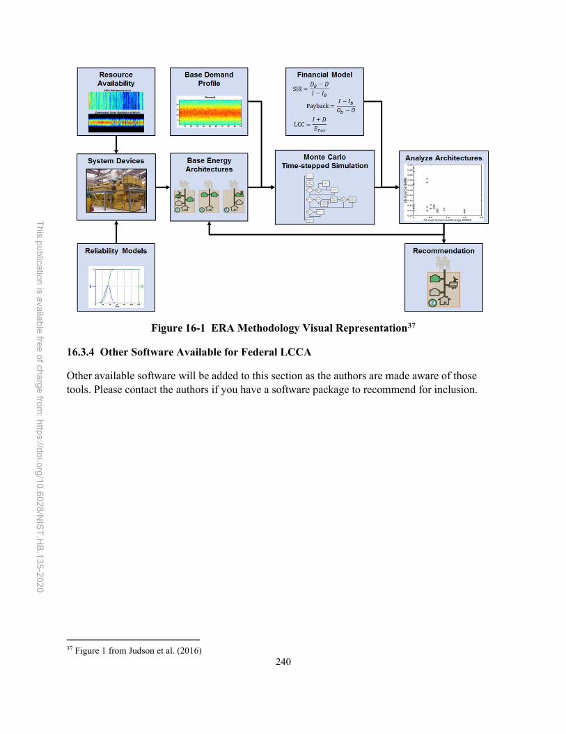
240

This p

ublica

tion is ava

ilab

le free

of ch

arge

from: h

ttps://doi.o

rg/1

0.6

028

/NIS

T.H

B.13

5-202

0

Figure 16-1 ERA Methodology Visual Representation37

16.3.4 Other Software Available for Federal LCCA

Other available software will be added to this section as the authors are made aware of those tools. Please contact the authors if you have a software package to recommend for inclusion.

37 Figure 1 from Judson et al. (2016)

241

This p

ublica

tion is ava

ilab

le free

of ch

arge

from: h

ttps://doi.o

rg/1

0.6

028

/NIS

T.H

B.13

5-202

0

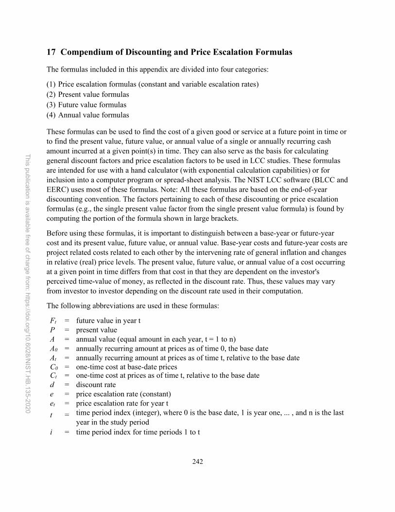
242

This p

ublica

tion is ava

ilab

le free

of ch

arge

from: h

ttps://doi.o

rg/1

0.6

028

/NIS

T.H

B.13

5-202

0

17 Compendium of Discounting and Price Escalation Formulas

The formulas included in this appendix are divided into four categories:

(1) Price escalation formulas (constant and variable escalation rates) (2) Present value formulas (3) Future value formulas (4) Annual value formulas

These formulas can be used to find the cost of a given good or service at a future point in time or to find the present value, future value, or annual value of a single or annually recurring cash amount incurred at a given point(s) in time. They can also serve as the basis for calculating general discount factors and price escalation factors to be used in LCC studies. These formulas are intended for use with a hand calculator (with exponential calculation capabilities) or for inclusion into a computer program or spread-sheet analysis. The NIST LCC software (BLCC and EERC) uses most of these formulas. Note: All these formulas are based on the end-of-year discounting convention. The factors pertaining to each of these discounting or price escalation formulas (e.g., the single present value factor from the single present value formula) is found by computing the portion of the formula shown in large brackets.

Before using these formulas, it is important to distinguish between a base-year or future-year cost and its present value, future value, or annual value. Base-year costs and future-year costs are project related costs related to each other by the intervening rate of general inflation and changes in relative (real) price levels. The present value, future value, or annual value of a cost occurring at a given point in time differs from that cost in that they are dependent on the investor's perceived time-value of money, as reflected in the discount rate. Thus, these values may vary from investor to investor depending on the discount rate used in their computation.

The following abbreviations are used in these formulas:

Ft = future value in year t P = present value A = annual value (equal amount in each year, t = 1 to n) A0 = annually recurring amount at prices as of time 0, the base date At = annually recurring amount at prices as of time t, relative to the base date C0 = one-time cost at base-date prices Ct = one-time cost at prices as of time t, relative to the base date d = discount rate e = price escalation rate (constant) et = price escalation rate for year t

t = time period index (integer), where 0 is the base date, 1 is year one, ... , and n is the last year in the study period

i = time period index for time periods 1 to t

243

This p

ublica

tion is ava

ilab

le free

of ch

arge

from: h

ttps://doi.o

rg/1

0.6

028

/NIS

T.H

B.13

5-202

0

Note: If d is expressed in real terms (exclusive of general inflation) then e must also be expressed in real terms. If d is expressed in nominal (market) terms (inclusive of inflation) then e must also include general inflation.

17.1 Price Escalation Formulas

Price escalation formulas are used to find a future cost of a good or service at the end of the nth time period (usually years), given its base-year cost and the annual rate of price escalation for that commodity. If the analysis is conducted in constant dollars, the price escalation rate should be expressed in real terms (exclusive of general inflation); if the analysis is conducted in current dollars, the price escalation rate should be expressed in nominal terms (inclusive of general inflation).

17.1.1 Constant Escalation Rate

Application: to find Ct when C0 is known and e is constant from year to year.

Formula:

𝐶 = 𝐶 ∙ (1 + 𝑒) (12 − 1)

Example:

C0 = $1000 e = 3 % t = 10

𝐶 = 1000 ∙ (1 + 0.03) = $1344 (12 − 2)

17.1.2 Variable Escalation Rate

Application: to find Ct when C0 is known and e varies from year to year.

Formula:

𝐶 = 𝐶 ∙ (1 + 𝑒) (12 − 3)

Example:

C0 = $1000 e1 = 1 % e2 = 2 % e3 = 3 % e4 = 4 % e5 = 5 % t = 5

244

This p

ublica

tion is ava

ilab

le free

of ch

arge

from: h

ttps://doi.o

rg/1

0.6

028

/NIS

T.H

B.13

5-202

0

𝐶 = 1000 ∙ (1 + 𝑒 ) ∙ (1 + 𝑒 ) ∙ (1 + 𝑒 ) ∙ (1 + 𝑒 ) ∙ (1 + 𝑒 )

= 1000 ∙ (1 + 0.01) ∙ (1 + 0.02) ∙ (1 + 0.03) ∙ (1 + 0.04) ∙ (1 + 0.05)

= $1159 (12 − 3)

17.2 Present Value Formulas

Present value formulas are used to find the present value of future amounts, when discount rate and the number of time periods (usually years) between the present time and the time of payment are known.

17.2.1 One-Time Amounts

17.2.1.1 Single Present Value (SPV) Formula

Application: to find P when amount at end of year t is known.

Formula:

𝑃 = 𝐶 ∙1

(1 + 𝑑) (12 − 4)

Example:

C10 = $1000 d = 5 % t = 10

𝑃 = 1000 ∙1

(1 + 0.05)= $614 (12 − 5)

17.2.1.2 Modified Single Present Value (SPV*) Formula

Application: to find P when the amount at the end of year t is expressed in base-year dollars (C0) and the price escalation rate is known.

Formula (constant e):

𝑃 = 𝐶 ∙1 + 𝑒

1 + 𝑑 (12 − 6)

Example:

C10 = $1000 e = 3 % d = 5 % t = 10

𝑃 = 1000 ∙1 + 0.03

1 + 0.05= $825 (12 − 7)

245

This p

ublica

tion is ava

ilab

le free

of ch

arge

from: h

ttps://doi.o

rg/1

0.6

028

/NIS

T.H

B.13

5-202

0

Formula (variable e):

𝑃 = 𝐶 ∙∏ (1 + 𝑒)

(1 + 𝑑)(12 − 8)

Example:

C0 = $1000 e1 = 1 % e2 = 2 % e3 = 3 % e4 = 4 % e5 = 5 % d = 5 % t = 5

𝑃 = 𝐶 ∙(1 + 𝑒 ) ∙ (1 + 𝑒 ) ∙ (1 + 𝑒 ) ∙ (1 + 𝑒 ) ∙ (1 + 𝑒 )

(1 + 𝑑)

=(1 + 0.01) ∙ (1 + 0.02) ∙ (1 + 0.03) ∙ (1 + 0.04) ∙ (1 + 0.05)

(1 + 0.05)= $908 (12 − 9)

17.2.2 Annually Recurring Amounts

When costs occur on an annual basis, whether constant or changing at a known rate, the present value of each annual cost over a given number of years can be calculated with a single equation using Uniform Present Value (UPV) factors.

Note: In the formulas for annually recurring amounts shown in Section 17.2.2, the number of time periods (n) can only be set to integer values. For time periods with decimal fractions, the present value of the cost incurred during the fractional time period must be calculated separately and added to the present value of the costs incurred during the integer time period.

17.2.2.1 Uniform Present Value (UPV) Formula and Factor

Application: to find P when A is known and constant.

Formula:

𝑃 = 𝐴0 ∙ (1 + 𝑑)𝑛 − 1

𝑑 ∙ (1 + 𝑑)𝑡(12 − 10)

Example:

A0 = $1000 d = 5 % t = 10

𝑃 = 𝐴0 ∙ (1 + 0.05)10 − 1

0.05 ∙ (1 + 0.05)10(12 − 11)

246

This p

ublica

tion is ava

ilab

le free

of ch

arge

from: h

ttps://doi.o

rg/1

0.6

028

/NIS

T.H

B.13

5-202

0

17.2.2.2 Modified Uniform Present Value (UPV*) Formula and Factors

Application: to find P when A is known but varies from time period to time period at a constant escalation rate (e) or at a changing escalation rate (ei).

Formula (constant e):

𝑃 = 𝐴0 ∙(1 + 𝑒)

(𝑑 − 𝑒)∙ 1 −

1 + 𝑒

1 + 𝑑

𝑛

(12 − 12)

Example:

A0 = $1000 e = 3 % d = 5 % n = 10

𝑃 = 1000 ∙(1 + 0.03)

(0.05 − 0.03)∙ 1 −

1 + 0.03

1 + 0.05

10

= $9010 (12 − 13)

Formula (variable e):

𝑃 = 𝐴 ∙∏ (1 + 𝑒 )

(1 + 𝑑)(12 − 14)

Example:

C0 = $1000 e1 = 1 % e2 = 2 % e3 = 3 % n = 3 d = 5 %

𝑃 = 1000 ∙1.01

(1.05)+

(1.01) ∙ (1.02)

(1.05)+

(1.01) ∙ (1.02) ∙ (1.03)

(1.05)= $2813 (12 − 14)

17.3 Future Value Formulas

Future value formulas are used to find the cost at some future point in time (t) of a good or service when the cost of that good or service at the base date, the price escalation rate, and the number of time periods (usually years) between the base date and the future date are known. Only one future value formula is presented here, the single compound amount formula.

Application: to find the future value at time ti (Ft2) of an amount paid at time t1 (Ct1), where t2 > t1.

Formula:

247

This p

ublica

tion is ava

ilab

le free

of ch

arge

from: h

ttps://doi.o

rg/1

0.6

028

/NIS

T.H

B.13

5-202

0

𝐹 = 𝐶 ∙ (1 + 𝑑) (12 − 15)

Example:

C10 = $1000 d = 5 % t1 = 5

t2 = 10

𝐹 = 1000 ∙ (1 + 0.05) = $1276 (12 − 16)

17.4 Annual Value Formula

The Annual-Value formula is used to determine an equal payment per time period (usually years) which is equivalent to a one-time cost or a stream of costs incurred during the same time period, given the time value of money as reflected in the discount rate (d). The Uniform Capital Recovery (UCR) factor can be used to calculate this annual value, given the present value of a cost or of a stream of costs computed using the same discount rate.

Uniform Capital Recovery (UCR) formula application: to find A when P is known.

Formula:

𝐴 = 𝑃 ∙𝑑 ∙ (1 + 𝑑)𝑛

(1 + 𝑑)𝑛 − 1(12 − 17)

Example:

P = $1000 d = 5 % n = 10

𝐴 = 1000 ∙0.05 ∙ (1 + 0.05)10

(1 + 0.05)10 − 1= $130 (12 − 18)

Note: Any single cost or stream of uneven costs over a given time period can be annualized over that time period by first finding the present value of that cost or stream of costs and then applying the UCR formula. For a stream of equal costs occurring in each time period over a given study period, the annualized cost is identical to that periodic cost when the same discount rate and study period are used.

248

This p

ublica

tion is ava

ilab

le free

of ch

arge

from: h

ttps://doi.o

rg/1

0.6

028

/NIS

T.H

B.13

5-202

0

18 Glossary

Because the function of this handbook is to explain and help implement the FEMP LCC Rules, terminology and definitions used in the Rules are presented here. Definitions of additional economic terms used in this handbook are also provided. These terms are defined from the perspective of implementing the FEMP LCC Rules. Defined terms that appear in the definitions of other terms are capitalized.

Adjusted Internal Rate of Return (AIRR) - Annual yield from a project over the Study Period, considering reinvestment of interim returns.

Alternative – project option that is to be compared to the Base Case.

Annually Recurring Costs -Those costs which are incurred each year in an equal amount throughout the Study Period, or which change from year to year at a known rate.

Uniform Capital Recovery (UCR) Factor - A discount factor by which a present dollar amount may be multiplied to find its equivalent Annual Value, based on a given Discount Rate and a given period.

Base/Baseline Case - The building, facility, or campus design against which an alternative design is compared.

Base Date - The beginning of the first year of the Study Period, generally the date on which the Life-Cycle-Cost analysis is conducted.

Base Year - The first year of the Study Period, generally the year in which the Life-Cycle-Cost Analysis is conducted.

Base-Date Price - The price of a good or service as of the Base Date.

Benefit-Cost Analysis – a method of evaluating projects or investments by comparing the present value or annual value of expected benefits to the present value of expected costs.

Benefit-Cost Ratio – benefits divided by costs, where both are discounted to a present value or equivalent uniform annual value.

Breakeven Analysis – a technique for determining that value of a variable which results in benefits (savings) just equal to costs.

Building Economics – the description and analysis of the production, distribution, and consumption of building-related goods and services

Building Technology - the technical processes and methods used in the constructing and operating buildings

Capital Investment Costs - Costs which are paid from capital funding accounts rather than from agency operating funds. For projects subject to the FEMP Rules, these include initial investment, capital replacements, and residual values.

249

This p

ublica

tion is ava

ilab

le free

of ch

arge

from: h

ttps://doi.o

rg/1

0.6

028

/NIS

T.H

B.13

5-202

0

Cash Flow - The stream of costs and savings (expressed for the purpose of this requirement in Constant Dollars) resulting from a project investment.

Conservation - prevention of wasteful use of a resource (e.g., energy, water)

Constant Dollars - Dollars of uniform purchasing power tied to a reference year (usually the Base Year) and exclusive of general price inflation or deflation.

Cost Effective - The condition in which an alternative saves more than it costs over the Study Period, where all Cash Flows are Discounted to their equivalent value at a common point in time.

Current Dollars - Dollars of nonuniform purchasing power, including general price inflation or deflation, in which actual prices are stated. (With zero inflation or deflation, current dollars are identical to constant dollars.)

Demand Charge - That portion of the charge for electric service based on fixed plant, equipment, and transmission costs associated with providing maximum required capacity.

Discount Factor - A multiplicative number used to convert a Cash Flow occurring at a given point in time (usually in the future) to its equivalent value at a common point in time (usually the Base Date).

Discount Formula - An expression of a mathematical relationship which enables the conversion of dollars at a given point in time to their equivalent amount at some other point in time.

Discount Rate - The rate of interest, reflecting the investor's Time Value of Money (or opportunity cost), that is used in Discount Formulas or to select Discount Factors which in turn are used to convert ("discount") Cash Flows to a common time. Real Discount Rates reflect Time Value of Money apart from changes in the purchasing power of the dollar and are used to discount Constant Dollar Cash Flows; Nominal Discount Rates include changes in the purchasing power of the dollar and are used to discount Current Dollar Cash Flows.

Discounted Payback (DPB) Period - The time required for the cumulative savings from an investment to pay back the Investment Costs and other accrued costs, considering the Time Value of Money.

Discounting - A technique for converting Cash Flows occurring over time to time-equivalent values, at a common point in time, adjusting for the Time Value of Money.

Economic Analysis - assessing or examining topics or issues from an economic perspective to optimize the use of scare resources

Energy Conservation Measure - An installation or modification of an installation in a facility which is primarily intended to reduce energy consumption cost or allow the use of a renewable energy source.

Energy Cost - The annual cost of fuel or energy used to operate a building or building system, as billed by the utility or supplier (including Demand Charges, if any). Energy Costs are incurred

250

This p

ublica

tion is ava

ilab

le free

of ch

arge

from: h

ttps://doi.o

rg/1

0.6

028

/NIS

T.H

B.13

5-202

0

during the Service Period only. Energy consumed in the construction or installation of a new building or building system is not included in this cost.

Escalation Rate - The rate of change in price for a good or service (as contrasted with the Inflation Rate, which is for all goods and services). See Real Escalation Rate and Nominal Escalation Rate.

Future Value - The time-equivalent value of past, present, or future Cash Flows expressed as of some future point in time.

Incremental Cost/Benefit – the additional cost (benefit) resulting from an increase in the investment in a project.

Inflation - A rise in the general price level, i.e., the price level for all goods and services. (A negative change in the general price level is called "Deflation.")

Initial Investment Costs - The initial costs of design, engineering, purchase and installation, exclusive of "Sunk Costs," all of which are assumed to occur as a lump sum at the beginning of the Base Year or phased in during the Planning/Construction Period.

Internal Rate of Return (IRR) - Annual yield from a project over the Study Period, i.e., the compound rate of interest which, when used to discount Cash Flows of an Alternative, will result in zero Net Savings (Net Benefits).

Investment Costs - The Initial Investment Cost of a building or building system and capital Replacement Costs, less Residual Value, plus Disposal Cost, if any.

Life-Cycle Cost (LCC) - The total discounted dollar costs of owning, operating, maintaining, and disposing of a building or building system over the appropriate Study Period (see Life-Cycle Cost Analysis).

Life-Cycle Cost Analysis (LCCA) - A general approach to economic evaluation that encompasses several related economic evaluation measures, including Life-Cycle Cost (LCC), Net Benefits (NB) or Net Savings (NS), Savings-to-Investment Ratio (SIR), and Adjusted Internal Rate of Return (AIRR), all of which take into account all dollar costs related to owning, operating, maintaining, and disposing of a project over the appropriate Study Period.

Measures of Economic Evaluation -The various ways in which project cash flows can be combined and presented to describe a measure of project cost effectiveness. The measures used to evaluate FEMP projects are Life-Cycle Cost (LCC), Net Savings (NS), Savings-to-Investment Ratio (SIR), Adjusted Internal Rate of Return (AIRR). Discounted Payback (DPB) and Simple Payback (SPB) are measures of evaluation not fully consistent with the LCCA but are used as supplementary measures in some federal programs.

Minimum Acceptable Rate of Return – the minimum percentage return required for an investment to be economically acceptable.

251

This p

ublica

tion is ava

ilab

le free

of ch

arge

from: h

ttps://doi.o

rg/1

0.6

028

/NIS

T.H

B.13

5-202

0

Modified Uniform Present Value (UPV*) Factor - A discount factor used to convert an annual amount, changing from year to year at a given escalation rate, to a time-equivalent Present Value. The FEMP UPV* Factor indicates a discount factor published in the Annual Supplement to Handbook 135 for use in computing present-value energy costs, based on energy price escalation rates provided for this purpose by DOE's Energy Information Administration.

Mutually Exclusive Projects - Projects where the acceptance of one precludes acceptance of the others.

Net Savings (NS) or Net Benefits (NB) - Time-adjusted savings or benefits less time- adjusted differential costs taken over the Study Period, for an Alternative relative to the Base Case.

Nominal Discount Rate - The rate of interest (market interest rate) reflecting the time value of money stemming from both inflation and the real earning power of money over time.

Nominal Escalation Rate - The projected annual rate of change in actual (market) prices for a good or service.

Operating, Maintenance, and Repair (OM&R) Costs - Non-investment costs related to the use of a building or building system, including energy and water costs.

Planning/Construction (P/C) Period - The period beginning with the Base Date and continuing up to the Service Date during which only Initial Investment Costs are incurred.

Present Value -The time-equivalent value of past, present or future Cash Flows as of the beginning of the Base Year.

Present Value Factor - A discount factor by which a future dollar amount may be multiplied to find its equivalent Present Value as of the Base Date. Single Present Value Factors are used to convert single future amounts to Present Values. Uniform Present Value Factors and Modified Present Value Factors are used to convert Annually Recurring amounts to Present Values.

Public Building - any building that is accessible to the public and is funded from public sources

Real Discount Rate - The rate of interest reflecting the portion of the time value of money attributable to the real earning power of money over time and not to general price inflation.

Real Escalation Rate - The difference between the rate of annual price change for a good or service and the rate of general Inflation.

Renewable Energy - Energy obtained from sources that are essentially inexhaustible (unlike, for instance, fossil fuels of which there is a limited supply). Renewable sources of energy include wind energy, geothermal energy, hydroelectric energy, photovoltaic and solar energy, biomass, and waste.

Replacement Costs - Capital costs incurred to replace the project during the Study Period. Sometimes referred to as Capital Replacement Costs. Replacement costs as used in this

252

This p

ublica

tion is ava

ilab

le free

of ch

arge

from: h

ttps://doi.o

rg/1

0.6

028

/NIS

T.H

B.13

5-202

0

handbook do not include the cost of replacing system components that are paid out of current operating budgets; these are Operation-Related Costs.

Residual Value - The estimated value, net of any Disposal Costs, of any building or building system removed or replaced during the Study Period, or remaining at the end of the Study Period, or recovered through resale or reuse at the end of the Study Period (also called Resale Value, Salvage Value, or Retention Value).

Resilience - the capacity to recover quickly from difficulties (e.g., disaster recovery)

Resource Economics – the description and analysis of the production, distribution, and consumption of natural resources (e.g., energy, water)

Retrofit - The installation of an Alternative into an existing facility.

Risk Attitude - The willingness of decision makers to take chances or to gamble on investments of uncertain outcome. Risk attitudes are generally classified as risk-averse, risk-neutral, or risk-taking.

Risk Exposure - The probability of investing in a project whose economic outcome is less favorable than what is economically acceptable.

Savings-to-Investment Ratio (SIR)- A ratio of economic performance computed from a numerator of discounted energy and/or water savings, plus (less) savings (increases) in other operation- related costs, and a denominator of increased Initial Investment Costs plus (less) increased (decreased) Replacement Costs, net of Residual Value (all in present-value terms), for an Alternative as compared with a Base Case.

Sensitivity Analysis - Testing the outcome of an evaluation to changes in the values of one or more system parameters from the initially assumed values.

Service Date - The point in time during the Study Period when a building or building system is put into use, and operation-related costs (including energy and water costs) begin to be incurred.

Service Period - The period starting with the Service Date and continuing through the end of the Study Period.

Simple Payback (SPB) Period -A measure of the length of time required for the cumulative savings from a project to recover its Initial Investment Cost and other accrued costs, without considering the Time Value of Money. SPB is usually measured from the Service Date of a project.

Single Present Value (SPV) Factor - The discount factor used to convert single future benefit and cost amounts to Present Value.

Study Period - The length of the time period covered by the economic evaluation. This includes both the Planning/Construction Period and the Service Period.

253

This p

ublica

tion is ava

ilab

le free

of ch

arge

from: h

ttps://doi.o

rg/1

0.6

028

/NIS

T.H

B.13

5-202

0

Sunk Costs - Costs which have been incurred or committed to prior to the Life-Cycle Cost analysis. These costs should not be considered in making a current project decision.

Sustainability - the ability to be maintained at a certain rate or level (e.g., building performance)

Time-of-Use Rate - Charges for service (usually electricity) that vary from period to period, based on the cost of supplying the service during that period.

Time-Value of Money - The time-dependent value of money, reflecting the opportunity cost of capital to the investor during that period. See Discount Rate.

Uncertainty – lack of certain, deterministic, values for the variable inputs used in an economic analysis.

Uniform Present Value (UPV) Factor - The discount factor used to convert uniform annual values to a time-equivalent Present Value.

UsefuI Life - The period over which a facility or facility system continues to generate benefits or savings.

254

This p

ublica

tion is ava

ilab

le free

of ch

arge

from: h

ttps://doi.o

rg/1

0.6

028

/NIS

T.H

B.13

5-202

0

References

Title 10 PART I — ORGANIZATION AND GENERAL MILITARY POWERS Chapter 1 - Definitions (e) Facilities and Operations (6) Energy Resilience, (2011).

Anderson, K., Burman, K., Simpkins, T., Helson, E., Lisell, L., & Case, T. (2016). New York Solar Smart DG Hub-Resilient Solar Project: Economic and Resiliency Impact of PV and Storage on New York Critical Infrastructure. Retrieved from https://www.nrel.gov/docs/fy16osti/66617.pdf:

Aroul, R., & Hansz, J. A. (2012). The Value of" Green:" Evidence from the First Mandatory Residential Green Building Program. Journal of Real Estate Research, 34(1), 27-49.

ASTM. (2015). Standard Guide for Selecting Techniques for Treating Uncertainty and Risk in the Economic Evaluation of Buildings and Building Systems, ASTM Designation E1369-15. Retrieved from West Conshohocken, PA:

ASTM. (2015e). Standard Classification for Building Elements and Related Sitework—UNIFORMAT II, ASTM Designation E1557 – 09. Retrieved from West Conshohocken, PA:

ASTM. (2016). Standard Practice for Applying Analytical Hierarchy Process (AHP) to Multiattribute Decision Analysis of Investments Related to Projects, Products, and Processes, ASTM Designation E1765-16. Retrieved from West Conshohocken, PA:

ASTM. (2017a). E917 - Standard Practice for Measuring Life-Cycle Costs of Buildings and Building Systems. Retrieved from West Conshohocken, PA:

ASTM. (2017b). E1074 - Practice for Measuring Net Benefits and Net Savings for Investments in Buildings and Building Systems. Retrieved from West Conshohocken, PA:

ASTM. (2017c). E1121 - Practice for Measuring Payback for Investments in Buildings and Building Systems. Retrieved from West Conshohocken, PA:

ASTM. (2017d). E1185 - Standard Guide for Selecting Economic Methods for Evaluating Investments in Buildings and Building Systems. Retrieved from West Conshohocken, PA:

ASTM. (2017e). E1057 - Practice for Measuring Internal Rate and Adjusted Internal Rate of Return for Investments in Buildings and Building Systems. Retrieved from West Conshohocken, PA:

ASTM. (2017f). E964 - Practice for Measuring Benefit-to-Cost and Savings-to-Investment Ratios for Buildings and Building Systems. Retrieved from West Conshohocken, PA:

ASTM E3130. (2018). Standard Guide for Developing Cost-Effective Community Resilience Strategies. In. https://www.astm.org/Standards/E3130.htm: ASTM International.

255

This p

ublica

tion is ava

ilab

le free

of ch

arge

from: h

ttps://doi.o

rg/1

0.6

028

/NIS

T.H

B.13

5-202

0

Barbose, G., Goldman, C., & Neenan, B. (2004). A Survey of Utility Experience with Real Time Pricing Retrieved from http://eta-publications.lbl.gov/sites/default/files/report-lbnl-54238.pdf

Baxter, J. (2018). Seminar on Department of Defense Energy Resilience. Presentation to the Federal Utility Partnership Working Group on April 20, 2018

Bleyl, J. W., Bareit, M., Casas, M. A., Chatterjee, S., Coolen, J., Hulshoff, A., . . . Ürge-Vorsatz, D. (2019). Office building deep energy retrofit: life cycle cost benefit analyses using cash flow analysis and multiple benefits on project level. Energy Efficiency(12), 261–279. doi:https://doi.org/10.1007/s12053-018-9707-8

Bond, S. A., & Devine, A. (2016). Certification Matters: Is Green Talk Cheap Talk? J Real Estate Finan Econ, 52, 117–140.

Bower, A. E., Bryan, K. E., Canada, K. J., Carter, K. A., & Watts, L. M. (2019). High-Performance Building Certification System Review. Retrieved from https://www.gsa.gov/about-us/organization/office-of-governmentwide-policy/office-of-federal-highperformance-buildings/policy/highperformance-building-certification-system-review

Bragera, G. S., & deDear, R. J. (1998). Thermal adaptation in the built environment: a literature review. Energy and Buildings, 27(1), 83-96.

Bureau of Labor Statistics. (2013). Green Goods and Services. Retrieved from https://www.bls.gov/ggs/

Carmichael, C., Porst-Hydras, K., Smidt, R., & Robinson-Freeman, Y. (2017). Deep Energy Retrofits. Paper presented at the Energy Exchange, Tampa, Florida.

Castillo, A. (2017). OSD Energy Resilience Overview - Energy Planning for Resilient Military Installations. https://www.acq.osd.mil/eie/Downloads/IE/20171205%20Energy%20Planning%20for%20Resilient%20Military%20Installations.pdf

CEQ. (2006). FEDERAL LEADERSHIP IN HIGH PERFORMANCE and SUSTAINABLE BUILDINGS MEMORANDUM OF UNDERSTANDING. Retrieved from https://www.wbdg.org/FFC/FED/HPSB-MOU.pdf

CEQ. (2008). HIGH PERFORMANCE and SUSTAINABLE BUILDINGS GUIDANCE. Retrieved from http://www.wbdg.org/FFC/FED/hpsb_guidance.pdf

CEQ. (2014). Updated Principles, Requirements and Guidelines for Water and Land Related Resources Implementation Studies.

CEQ. (2016). Guiding Principles for Sustainable Federal Buildings and Associated Instructions. Retrieved from

256

This p

ublica

tion is ava

ilab

le free

of ch

arge

from: h

ttps://doi.o

rg/1

0.6

028

/NIS

T.H

B.13

5-202

0

https://www.sustainability.gov/pdfs/guiding_principles_for_sustainable_federal_buildings.pdf

CEQ. (2019a). Federal Government-Wide Performance Data.

CEQ. (2019b). Implementing Instructions for Executive Order 13834 Efficient Federal Operations. Retrieved from https://www.sustainability.gov/pdfs/eo13834_instructions.pdf

CEQ. (2019c). Resources and Guidance for Federal Agencies - Council on Environmental Quality Guidance. Retrieved from https://www.sustainability.gov/resources.html

CFR. (2018). 10 Code of Federal Regulations (CFR) 436, Subpart A, Methodology and Procedures for Life-Cycle Cost Analysis. https://www.ecfr.gov/cgi-bin/text-idx?SID=1772217352e2b3956b37b48739ebd676&mc=true&node=pt10.3.436&rgn=div5

Charette, R. P., & Marshall, H. E. (1999). UNIFORMAT II elemental classification for building specifications, cost estimating, and cost analysis: US Department of Commerce, Technology Administration, National Institute of Standards and Technology.

Chen, D. G., & Chen, J. D. E. (2017). Monte-Carlo simulation-based statistical modeling: Springer.

Coleman, P. (2015). Escalation Rates in Energy Savings Performance Contracts. Energy Engineering, 112(5).

Coleman, P., Earni, S., & Williams, C. (2014). Could what that ESCO sales rep said really be true? Savings realization rates in ESPC versus bid-to-spec projects. Retrieved from

CRS. (2018). Energy Savings Performance Contracts (ESPCs) and Utility Energy Service Contracts (UESCs). Retrieved from

Dagpunar, J. S. (2007). Simulation and Monte Carlo: With applications in finance and MCMC: John Wiley & Sons.

DoD. (2014). DoD Product Support Business Case Analysis Guidebook - Introduction to the Product Support BCA. Retrieved from Washington, DC, USA: https://acc.dau.mil/bca-guidebook

DoD. (2015). Net Zero: Guide to Renewable ECIP Projects. https://www.energy.gov/eere/femp/downloads/army-net-zero-guide-renewable-energy-conservation-investment-program-ecip: NREL on behalf of U.S. Department of Defense (DoD)

DoD. (2017a). ENERGY RESILIENCE AND CONSERVATION INVESTMENT PROGRAM (ERCIP) GUIDANCE. https://www.acq.osd.mil/eie/IE/FEP_ECIP.html: Office of the Assistant Secretary of Defense for Sustainment

257

This p

ublica

tion is ava

ilab

le free

of ch

arge

from: h

ttps://doi.o

rg/1

0.6

028

/NIS

T.H

B.13

5-202

0

DoD. (2017b). INFLATION AND ESCALATION BEST PRACTICES FOR COST ANALYSIS: ANALYST HANDBOOK. Retrieved from

DoD. (2018). Department of Defense Instruction Number 4170.11 - Installation Energy Management. https://www.esd.whs.mil/Portals/54/Documents/DD/issuances/dodi/417011p.pdf?ver=2018-11-07-083917-293

DoD. (2019). Energy Management Reports.

Dodge Data & Analytics. (2018). World Green Building Trends 2018. Retrieved from https://www.worldgbc.org/news-media/world-green-building-trends-2018-smartmarket-report:

DOE. (2015). Interruption Cost Estimate (ICE) Calculator.

DOE. (2019a). Comprehensive Annual Energy Data and Sustainability Performance.

DOE. (2019b). EnergyPlus Simulation SoftwareVersion 9.0.1: U.S. Department of Energy, Building Technologies Program (BTP). Retrieved from https://energyplus.net/

DOE BTO. (2017). Utilizing Commercial Real Estate Owner and Investor Data to Analyze the Financial Performance of Energy Efficient, High-Performance Office Buildings. Retrieved from

E.O.13123. (1999). Greening the Government Through Efficient Energy Management.

E.O.13423. (2007). Strengthening Federal Environmental, Energy, and Transportation Management.

E.O.13693. (2015). Planning for Federal Sustainability in the Next Decade.

E.O.13834. (2018). Efficient Federal Operations.

EIA. (2019). Electric Power Monthly - Table 5.6.A. Average Price of Electricity to Ultimate Customers by End-Use Sector.

Eichholtz, P., Kok, N., & Quigley, J. M. (2010). Doing well by doing good? Green office buildings. The American Economic Review, 2492-2509.

Eichholtz, P., Kok, N., & Quigley, J. M. (2013). The economics of green building. Review of Economics and Statistics, 95(1), 50-63.

Environmental Protection Agency. (2018). Tool for the Reduction and Assessment of Chemical and other Environmental Impacts (TRACI) 2.1. Retrieved from https://www.epa.gov/chemical-research/tool-reduction-and-assessment-chemicals-and-other-environmental-impacts-traci

258

This p

ublica

tion is ava

ilab

le free

of ch

arge

from: h

ttps://doi.o

rg/1

0.6

028

/NIS

T.H

B.13

5-202

0

FEMP. (2005). Guidance on Life-Cycle Cost Analysis Required by Executive Order 13123. Federal Energy Management Program

FEMP. (2006). Performing Energy Security Assessments - A How-To Guide for Federal Facility Managers. https://www.energy.gov/eere/femp/downloads/performing-energy-security-assessments-how-guide-federal-facility-managers: Produced for the U.S. Department of Energy, Energy Efficiency and Renewable Energy, Federal Energy Management Program, by Oak Ridge National Laboratory.

FEMP. (2009). Practical Guide to Savings and Payments in FEMP ESPC Task Orders Rev. 3. Retrieved from https://www.energy.gov/sites/prod/files/2013/10/f3/practguide_sav_paymnts.pdf

FEMP. (2011a). Best Practices Guide for Energy-Efficient Data Center Design. Retrieved from

FEMP. (2011b). Funding Federal Energy and Water Projects. In E. E. R. E. U.S. Department of Energy (Ed.).

FEMP. (2017a). Utility Partnerships Program Overview. https://www.energy.gov/sites/prod/files/2017/08/f35/utility_program_2017_0.pdf

FEMP. (2017b). Water and Wastewater Annual Price Escalation Rates for Selected Cities across the United States. Retrieved from

FEMP. (2018). How to Determine and Verify Operating and Maintenance Savings in Federal Energy Savings Performance Contracts. Retrieved from https://www.energy.gov/eere/femp/downloads/how-determine-and-verify-operating-and-maintenance-savings-energy-savings:

FEMP. (2019a). Awarded DOE IDIQ Energy Savings Performance Contract Projects. Retrieved from https://www.energy.gov/eere/femp/awarded-doe-idiq-energy-savings-performance-contract-projects

FEMP. (2019b). Energy Savings Performance Contract ENABLE Energy Service Companies.

FEMP. (2019c). Federal Agency Use of Renewable Electric Energy.

FEMP. (2019d). Federal Energy Savings Performance Contracts - Frequently Asked Questions on the Scope of 42 U.S.C. § 8287 et. seq. https://www.energy.gov/sites/prod/files/2019/07/f64/espc-faq-42-usc-2019_0.pdf

FEMP. (2019e). Federal On-Site Distributed Energy Project Financing Options.

FEMP. (2019f). Guidance on Utility Rate Estimations and Weather Normalization in Performance Contracts. https://www.energy.gov/eere/femp/downloads/guidance-utility-rate-estimations-and-weather-normalization-performance

259

This p

ublica

tion is ava

ilab

le free

of ch

arge

from: h

ttps://doi.o

rg/1

0.6

028

/NIS

T.H

B.13

5-202

0

FEMP. (2020). Utility Energy Service Contract Guide: A Resource for Contracting Officers Working on UESC Projects.

Fuerst, F., & McAllister, P. (2011a). Green Noise or Green Value. Real Estate Economics, 39, 45-69. doi:10.1111/j.1540-6229.2010.00286.x

Fuerst, F., & McAllister, P. (2011b). The Impact of Energy Performance Certificates on the Rental and Capital Values of Commercial Property Assets. Energy Policy, 39, 6608-6614. doi:http://dx.doi.org/10.2139/ssrn.1839429

GAO. (2003). Federal Real Property. Retrieved from Washington, D.C.:

GAO. (2008). Federal Real Property: Government’s Fiscal Exposure from Repair and Maintenance Backlogs Is Unclear. Retrieved from Washington, D.C.:

GAO. (2009a). Federal Real Property: An Update on High Risk Issues. Retrieved from Washington, D.C.:

GAO. (2009b). GAO Cost Estimating and Assessment Guide - Best Practices for Developing and Managing Capital Program Costs. Retrieved from

GAO. (2014). Improved Transparency Could Help Efforts to Manage Agencies' Maintenance and Repair Backlogs. Retrieved from Washington, D.C.:

GAO. (2016). Defense Infrastructure - Energy conservation Investment Program Needs Improved Reporting, Measurement, and Guidance. (GAO-16-162). https://www.gao.gov/products/GAO-16-162

GAO. (2019). Substantial Efforts Needed to Achieve Greater Progress on High-Risk Areas. Retrieved from Washington, D.C.:

Gaskin, R. (2013). The big green opportunity for small business in the US: Small business sustainability report. Retrieved from http://biggreenopportunity.org/wp-content/uploads/2013/05/Big-Green-Opportunity-Report-FINAL-WEB.pdf

Gilbert, S. W., Butry, D. T., Helgeson, J. F., & Chapman, R. E. (2015). Community Resilience Economic Decision Guide for Buildings and Infrastructure Systems. Retrieved from

Giuseppe, E. D., Massi, A., & D’Orazio, M. (2017). Impacts of uncertainties in Life Cycle Cost analysis of buildings energy efficiency measures: application to a case study. Energy Procedia, 111, 442-451.

Greenberg, S., Sartor, D., & Tschudi, W. (2015). Example Data Center Energy Efficiency Assessment - Final Report. Retrieved from

GSA. (2011). Green building performance: A post occupancy evaluation of 22 GSA buildings. Retrieved from

260

This p

ublica

tion is ava

ilab

le free

of ch

arge

from: h

ttps://doi.o

rg/1

0.6

028

/NIS

T.H

B.13

5-202

0

GSA. (2012). Sustainable Building Study Using Whole-System and Life-Cycle Thinking. Retrieved from 2012 REPORT TO THE MID-ATLANTIC, REGION 3 OF THE U.S. GENERAL SERVICES ADMINISTRATION (GSA):

GSA. (2018). The Impact of High-Performance Buildings. Retrieved from

GSA. (2019). LEED Building Information.

H.R.6. (2005). Energy Policy Act of 2005. United States: 109th Congress

H.R.776. (1992). Energy Policy Act of 1992. In (102nd Congress ed., Vol. Public Law 102–486, 106 Stat. 2776). United States: Congress.

H.R.5037. (1978). Public Law 95-619 - National Energy Conservation Policy Act (NECPA).

Hall, J. A., Gill, S., Obeysekera, J., Sweet, W., Knuuti, K., & Marburger, J. (2016). Regional Sea Level Scenarios for Coastal Risk Management: Managing the Uncertainty of Future Sea Level Change and Extreme Water Levels for Department of Defense Coastal Sites Worldwide. Retrieved from

Helgeson, J. F., Webb, D. H., & Grubb, S. A. (2017). The Economic Decision Guide Software (EDGe$) Tool User Guidance. Retrieved from

Hoen, B., Adomatis, S., Jackson, T., Graff-Zivin, J., Thayer, M., Klise, G. T., & Wiser, R. (2015). SELLING INTO THE SUN: PRICE PREMIUM ANALYSIS OF A MULTI-STATE DATASET OF SOLAR HOMES. Retrieved from

IEA. (2017). Deep Energy Retrofit – Case Studies: Business and Technical Concepts for Deep Energy Retrofit

of Public Buildings. Retrieved from https://iea-annex61.org/files/results/Annex_61_SubTask_A_CaseStudies_2017-12-18.pdf:

IEEE. (2007). IEEE Gold Book - Std 493-2007 (Revision of IEEE Std 493-1997) - IEEE Recommended Practice for the Design of Reliable Industrial and Commercial Power Systems. In: Institute of Electrical and Electronics Engineers, Inc. (IEEE).

Revenue Procedure 2017-19, (2017).

Judson, N., Pina, A. L., Dydek, E. V., Broekhoven, S. B. V., & Castillo, A. S. (2016). Application of a Resilience Framework to Military Installations: A Methodology for Energy Resilience Business Case Decisions. Retrieved from https://apps.dtic.mil/dtic/tr/fulltext/u2/1024805.pdf:

Jungclaus, M., Carmichael, C., McClurg, C., Simmons, M., Smidt, R., Hydras, K. P., . . . Nasseri, C. (2017). Deep Energy Retrofits in Federal Buildings: The Value, Funding Models, and Best Practices. ASHRAE Transactions, 123, 55-70.

261

This p

ublica

tion is ava

ilab

le free

of ch

arge

from: h

ttps://doi.o

rg/1

0.6

028

/NIS

T.H

B.13

5-202

0

Kats, G., Alevantis, L., Berman, A., Mills, E., & Perlman, J. (2003). The costs and financial benefits of green buildings. A Report to California’s Sustainable Building Task Force. USA.

Kok, N., & Kahn, M. (2012). The Value of Green Labels in the California Housing Market: An Economic Analysis of the Impact of Green Labeling on the Sales Price of a Home. Retrieved from Berkely, CA:

Lavappa, P., & Kneifel, J. (2019). Energy Price Indices and Discount Factors for Life-Cycle Cost Analysis - 2019, Annual Supplement to NIST Handbook 135. (NISTIR 85-3273-34).

Loftness, V., Hartkopf, V., & Gurtekin, B. (2003). Linking energy to health and productivity in the built environment. Paper presented at the 2003 Greenbuild Conference.

Lohse, R., & Zhivov, A. (2019). Deep Energy Retrofit Guide for Public Buildings – Business and Financial Models.: Springer.

Marshall, H. E. (1988). Techniques for Treating Uncertainty and Risk in the Economic Evaluation of Building Investments. Retrieved from https://nvlpubs.nist.gov/nistpubs/Legacy/SP/nistspecialpublication757.pdf:

McGraw-Hill Construction. (2017). World Green Building Trends 2016: United States. Retrieved from

Murakami, K., Itsubo, N., Kuriyama, K., Yoshida, K., & Tokimatsu, K. (2018). Development of weighting factors for G20 countries. Part 2: estimation of willingness to pay and annual global damage cost. Int J Life Cycle Assess, 23, 2349-2364. doi:10.1007/s11367-017-1372-1

NIST. (2006a). Building Life-Cycle Cost" (BLCC) Computer Program. (NISTIR 5185-2).

NIST. (2006b). Energy Escalation Rate Calculator (EERC), , National Institute of Standards and Technology. (NISTIR 5186).

NRC. (2001). Deferred Maintenance Reporting for Federal Facilities: Meeting the Requirements of Federal Accounting Standards Advisory Board Standard Number 6, as Amended. Retrieved from Washington, DC:

NRC. (2012). Predicting Outcomes of Investments in Maintenance and Repair of Federal Facilities. Retrieved from Washington, DC:

NREL. (2019a). OpenStudio 2.7.0. Retrieved from https://www.openstudio.net

NREL. (2019b). REopt Lite.

NREL. (2019c). REopt: Renewable Energy Integration & Optimization.

262

This p

ublica

tion is ava

ilab

le free

of ch

arge

from: h

ttps://doi.o

rg/1

0.6

028

/NIS

T.H

B.13

5-202

0

OMB. (1992). GUIDELINES AND DISCOUNT RATES FOR BENEFIT-COST ANALYSIS OF FEDERAL PROGRAMS.

OMB. (2003). Circular A-4. https://www.whitehouse.gov/sites/whitehouse.gov/files/omb/circulars/A4/a-4.pdf

OMB. (2018a). DISCOUNT RATES FOR COST-EFFECTIVENESS ANALYSIS OF FEDERAL PROGRAMS: Revisions to Appendix C of OMB Circular A-94. 83 FR 5646

OMB. (2018b). PREPARATION, SUBMISSION, AND EXECUTION OF THE BUDGET. Retrieved from https://www.whitehouse.gov/wp-content/uploads/2018/06/a11.pdf

OMB M-12-21. (2012). Memorandum for Heads of Executive Departments and Agencies.

Paul, W. L., & Taylor, P. A. (2008). A comparison of occupant comfort and satisfaction between a green building and a conventional building. Building and Environment, 43(11), 1858-1870.

Pizzol, M., Weidema, B., Brand, M., & Osset, P. (2015). Monetary valuation in Life Cycle Assessment: a review. Journal of Cleaner Production, 86, 170-179. doi:http://dx.doi.org/10.1016/j.jclepro.2014.08.007

Ries, R., Bilec, M. M., Gokhan, N. M., & Needy, K. L. (2006). The Economic Benefits of Green Buildings: A Comprehensive Case Study. The Engineering Economist, 51(3), 259-295. doi:https://doi.org/10.1080/00137910600865469

RMI. (2015a). DEEP ENERGY RETROFITS USING ENERGY SAVINGS PERFORMANCE CONTRACTS: SUCCESS STORIES. Retrieved from

RMI. (2015b). THE PATH TO A DEEP ENERGY RETROFIT USING AN ENERGY SAVINGS PERFORMANCE CONTRACT. Retrieved from

Romm, J. J., & Browning, W. D. (1998). Greening the Building and the Bottom Line: Increasing Productivity Through Energy-Efficient Design. Retrieved from

Rubinstein, R. Y., & Kroese, D. P. (2016). Simulation and the Monte Carlo method (Vol. 10) John Wiley & Sons.

S.1382. (1988). Public Law 100-615 - Federal Energy Management Improvement Act.

Savena, M., Judson, N., & Pina, A. (2017). The Cost of Energy Security and Resilience. In. https://www.energy.gov/sites/prod/files/2017/11/f46/25-fupwgfall2017_savena_judson_pina_rev.pdf: 2017 Fall Federal Utility Partnership Working Group Seminar.

Shonder, J., & Atkin, E. (2005). Determining Price Reasonableness in Federal ESPCs. Retrieved from

263

This p

ublica

tion is ava

ilab

le free

of ch

arge

from: h

ttps://doi.o

rg/1

0.6

028

/NIS

T.H

B.13

5-202

0

Slattery, B. (2018). Reported Energy and Cost Savings from the DOE ESPC Program: FY 2016. Retrieved from https://www.energy.gov/eere/femp/downloads/reported-energy-and-cost-savings-espc-program

Sullivan, G. P., Pugh, R., Melendez, A. P., & Hunt, W. D. (2010). Operations & Maintenance Best Practices - A Guide to Achieving Operational Efficiency - Release 3.0. Retrieved from Pacific Northwest National Laboratory (PNNL):

Tri-Services. (1991). Criteria/Standards for Economic Analyses/Life Cycle Costing for MILCON Design. Memorandum of Agreement

H.R. 6: Energy Independence and Security Act (EISA) of 2007, P.L. 110-140 C.F.R. § 441 (2007).

U.S. Green Building Council. (2015). 2015 Green Building Economic Impact Study. Retrieved from https://www.usgbc.org

U.S. Green Building Council. (2017). LEED Projects and People Databases. Retrieved from https://www.usgbc.org

USACE. (2018). Energy Savings Performance Contracting Fact Sheet. Program Manager 256-895-1514 Retrieved from https://www.hnc.usace.army.mil/Media/Fact-Sheets/Fact-Sheet-Article-View/Article/484226/energy-division-energy-savings-performance-contracting-espc-program/

Wiley, J. A., Benefield, J. D., & Johnson, K. H. (2010). Green design and the market for commercial office space. The Journal of Real Estate Finance and Economics, 41(2), 228-243.

Wilson, E., Metzger, C., Horowitz, S., & Hendron, R. (2014). 2014 Building America House Simulation Protocols. Retrieved from Golden, CO: http://energy.gov/sites/prod/files/2014/03/f13/house_simulation_protocols_2014.pdf

Zhang, L., Wu, J., & Liu, H. (2018). Turning green into gold: A review on the economics of green buildings. Journal of Cleaner Production, 172, 2234-2245. doi:https://doi.org/10.1016/j.jclepro.2017.11.188

Zhivov, A. (2018). Technologies Integration to Achieve Resilient, Low-Energy Military Installations. Retrieved from

Zhivov, M. (2020). Enhanced Life Cycle Cost Analysis of Sustainable Office Buildings. ASHRAE Transactions, 126.