Life Cycle Environmental Impacts ofSelected U.S. Ethanol Productionand Use Pathways in 2022D A V I D D . H S U , * D A N I E L I N M A N ,G A R V I N A . H E A T H ,E D W A R D J . W O L F R U M ,M A R G A R E T K . M A N N , A N D A N D Y A D E N

National Renewable Energy Laboratory, 1617 Cole Boulevard,Golden, Colorado 80401-3393

Received January 18, 2010. Revised manuscript receivedMay 10, 2010. Accepted May 25, 2010.

Projected life cycle greenhouse gas (GHG) emissions andnet energy value (NEV) of high-ethanol blend fuel (E85) usedto propel a passenger car in the United States are evaluatedusing attributional life cycle assessment. Input data representnational-average conditions projected to 2022 for ethanolproduced from corn grain, corn stover, wheat straw, switchgrass,and forest residues. Three conversion technologies areassessed:advanceddrymill (corngrain),biochemical (switchgrass,corn stover, wheat straw), and thermochemical (forestresidues). A reference case is compared against results fromMonte Carlo uncertainty analysis. For this case, one kilometertraveledonE85fromthefeedstock-to-ethanolpathwaysevaluatedhas 43%-57% lower GHG emissions than a car operated onconventional U.S. gasoline (base year 2005). Differences in NEVcluster by conversion technology rather than by feedstock.The reference case estimates of GHG and NEV skew to the tailsof the estimated frequency distributions. Though not asoptimistic as the reference case, the projected median GHGand NEV for all feedstock-to-E85 pathways evaluated offersignificant improvementoverconventionalU.S.gasoline.Sensitivityanalysis suggests that inputs to the feedstock productionphase are the most influential parameters for GHG and NEV.Results from this study can be used to help focus research anddevelopment efforts.

Introduction

Forty-one billion liters of ethanol were produced in the UnitedStates in 2009, mostly from corn grain (Zea mays L.) (1). Aspart of a strategy to address national security, greenhousegas (GHG) emissions, and rural economic development, theEnergy Independence and Security Act of 2007 (EISA) (2)amended the 2005 renewable fuel standard (RFS) to mandatethat approximately 136 billion liters per year (bLy) beproduced by 2022. Under the 2007 RFS, a maximum of 56.6bLy of ethanol derived from conventional sources (e.g., corngrain) may qualify as a renewable fuel (2); the remaindermust be met by biofuel derived from second-generationfeedstocks, such as agricultural residues, forest residues, andperennial grasses.

Life cycle net energy value (NEV) and GHG emissionshave been used as metrics to compare different feedstock-

to-ethanol production systems and gasoline. With a fewexceptions (3, 4), most studies conclude that corn ethanolhas NEV and GHG advantages compared to gasoline (5-9).After harmonizing the methods of six previous life cycleassessments (LCA), Farrell and colleagues (10) found thatcurrent corn ethanol production yields an NEV of ap-proximately 5 MJ L-1 and a GHG intensity of -18%(uncertainty range: -36% to +29%) compared with that ofconventional gasoline. Similarly, ethanol derived from bothswitchgrass and corn stover has been shown to have higherNEV and lower GHG emissions when compared to gasoline(11, 12). An LCA consistently comparing multiple feedstocksin the same production year would contribute to currentresearch.

This study uses attributional LCA to compare projectedGHG emissions and NEV of ethanol-based transportationfuel derived from five feedstocks grown and used in theconterminous United States in 2022 to that of conventionalgasoline in 2005. Advanced designs for all life cycle stages ofa first-generation feedstock (corn grain) and four next-generation feedstocks (corn stover, wheat straw, switchgrass,and forest residues) are considered. Life cycle GHG and NEVof gasoline are considered for the base year of 2005, similarto the mandates in EISA. Because EISA and other environ-mental mandates demand performance often far beyondcurrent practice, this analysis aims to inform industrial andgovernmental research and development decisions by (1)determining the key input parameters that impact life cycleGHG emissions and NEV, and (2) quantifying the distributionof two environmental performance metrics. To do so,sensitivity and uncertainty analysis methods are applied.

Methods

SimaPro v.7.1 life cycle assessment modeling software (13)is used to develop and link unit processes. Most processesare custom created using primary, publicly available data. Inthe absence of such data, we use the Ecoinvent v.2.0 (14)and, to a lesser extent, the U.S. Life Cycle Inventory (U.S.LCI) (15) processes. For some processes that are developedfrom Ecoinvent and the U.S. LCI, we modify the former tobe reflective of U.S. conditions and the latter to account forembodied emissions and energy flows. This study followsInternational Organization for Standardization standards forLCA, including stakeholder and external reviews (16, 17); allprocesses underwent external review by experts from in-dustry, academia, and government.

Modeling Approach and Assumptions. The modelingboundary for this study is from field to wheels includingembodied energy and material flows. The functional unit is1 km traveled by a light-duty passenger car operated on E85in the year 2022. The ethanol is assumed to be produced inthe conterminous United States (18). For our reference case,E85 is assumed to be 78 v% ethanol and 22 v% conventionalunleaded gasoline, which includes gasoline denaturant (2v% of ethanol). (This composition is based on an average ofregional and seasonal blends (19)). The reference caseevaluated in this study is based on extrapolation of nationalaverage data and anticipated industry learning and im-provement. Therefore, the reference case is not necessarilyindicative of any region of the country. Sensitivity anduncertainty analyses explore the impact of variability (con-sidered on a national average basis) of a large set of inputparameters on projected GHG and NEV results.

Avoided impacts are accounted for using product dis-placement (boundary expansion) (16, 17). For products that

* Corresponding author e-mail: david.hsu@nrel.gov; phone: 303-384-6887; fax: 303-384-7449.

Environ. Sci. Technol. 2010, 44, 5289–5297

10.1021/es100186h 2010 American Chemical Society VOL. 44, NO. 13, 2010 / ENVIRONMENTAL SCIENCE & TECHNOLOGY 9 5289

Published on Web 06/07/2010

share inputs (e.g., corn grain and corn stover), burdens areallocated between products based on a “product-purpose”approach (20). For example, irrigation used in corn produc-tion is driven by the purpose of growing grain, not stover;consequently all irrigation inputs are allocated to the corngrain. Other allocation approaches (mass-based, energycontent-based) were investigated, and the effect that thesehad on GHG and NEV metrics does not change our overallconclusions. Impacts from infrastructure attributable to EISAare amortized over the lifetime of the infrastructure element.Inputs to multiyear cropping systems (i.e., switchgrass andforests) are likewise annualized by the length of the croppingrotation. Impacts from direct and indirect land use change(LUC) are not considered in this study. These impacts arepotentially large (e.g., 21, 22) and currently highly uncertain,but as will be shown from the results of this study,considerable uncertainty surrounds the direct emissions fromthe system as well. We focus on establishing the uncertaintyof direct emissions, which is foundational to understandingthe full consequences of ethanol production systems.

The sections below summarize the data sources, methods,and assumptions employed in the modeling of each life cyclestage. Additional information can be found in the SupportingInformation.

Feedstock Production. Feedstock production includes allprocesses from field preparation and planting throughharvest. Corn, corn stover, and wheat straw production arebased on projections of historical U.S. national average data(23) to the year 2022. Switchgrass production is based onpublished research from large-scale, long-term, on-farmstudies and reflects projected improvements in feedstockyield and management (24, 25) and an annual yield im-provement of 2%, which is well in line with the annualincrease expected from intensification (26). Forest residueproduction is based on modifications made to LCI datacollected from whole-tree timber harvesting operations (15).The reference case removal rate for both the corn stover andwheat straw is assumed to be 30 wt% of total residue (27).In the reference case, loss of stover as a livestock feedsupplement is modeled as being replaced by hay at a rate of0.174 kg hay per kg stover removed for ethanol production(28).

Corn and wheat are assumed to be harvested using asingle-pass harvest system (29). Switchgrass is assumed tobe harvested using an advanced, one-step process (29). Forestresidues, as modeled in this study, are assumed to be thenonmerchantable portions of the harvested tree that arebrought to the landing, typically discarded, and in many casesburned. Forest residue harvesting is modeled based on U.S.whole-tree logging operations (15). Four logging regions areconsidered: the Pacific Northwest, the Intermountain West,the Southeast, and the Northeast-North Central regions (15);only private and state-owned forests are considered. Forestresidues are assumed to be approximately 30% of the totalcut volume; of this volume, it is further assumed that 30%is lost during skidding operations. The four regions are usedto produce a weighted average, based on the regions’ long-term, average annual production (30). The accumulated forestresidues are assumed to be chipped at the landing usingstandard industrial chipping equipment.

Feedstock Preprocessing. Feedstock preprocessing is mod-eled to reflect an “Advanced Uniform-Format FeedstockSupply System” as described in the Idaho National Laboratoryfeedstock delivery design report (29). This feedstock supplysystem is modeled to provide a physically uniform feedstockto the biorefinery conversion facility, thereby minimizingfeedstock preprocessing at the biorefinery. The biomass isseparated from any grain, baled, and transported to apreprocessing facility where the biomass is dried, ground,and stored. The mass fractions of corn stover, switchgrass,

and wheat straw that need to be actively dried instead offield dried are set at 0.85, 0.15, and 0.1, respectively (31).

Forest residue harvest already includes a chipping opera-tion, therefore preprocessing only includes transport to astorage facility. Likewise, corn grain harvest includes separa-tion of the grain, so preprocessing only includes transportto a storage facility based on distances from Yu and Hart(32).

Feedstock Transport. This stage models the transport offeedstock from the preprocessing/storage facility to thebiorefinery. Distances are disaggregated by feedstock wherepossible (29, 33-35), otherwise recent corn grain logisticsare assumed (36-38). Allocation to truck, rail, or bargetransportation is based on previous experience assumingthat a future system will be largely similar (36-38).

Conversion. While no commercial-scale cellulosic ethanolfacilities exist today, conceptual designs, as documented inNREL reports, define the 2022 reference case cellulosicethanol conversion processes. Biochemical production ofethanol, applied to corn stover, switchgrass, and wheat straw,is through dilute acid pretreatment, enzymatic hydrolysis,and fermentation (39); thermochemical production of etha-nol, applied to forest residues, is via indirect gasification andmixed alcohol synthesis (40). Herbaceous feedstock com-positions are based on distributional information from Leeet al. (41).

Corn dry mill mass balances are based on a 151 millionliter ethanol per year version of a corn dry mill Aspen Plusmodel (42). The 2022 version of the corn dry mill is basedon projected process heat and electricity mix, along withincreased plant efficiencies, from a study by Mueller (43).The primary energy source for heat and power for corn drymills is expected to shift from 97% fossil fuels (93% naturalgas and 4% coal) in 2005 to 64% (60% natural gas and 4%coal) in 2022, with the remainder coming from renewablebiomass and biogas power sources. In addition, the advancedcorn grain case included increased ethanol yields based onArgonne National Laboratory’s GREET model (38).

Enzymes used in the corn dry mill plant and thebiochemical conversion process are based on informationfrom Novozymes (44, 45). The biochemical conversionprocess exports electricity, which is assumed to displace U.S.grid electricity (46). The thermochemical conversion processproduces mixed alcohols as a coproduct, which could beused in the chemical or fuel market; the LCI for thethermochemical conversion process is allocated betweenethanol and mixed alcohols on an energy content basis. Corndry mill plants produce distillers dried grains with solubles(DDGS). In this study, DDGS is assumed to be a marketableanimal feed replacement. To account for this, the systemboundaries are expanded to include displaced soy, corn, andurea production, as well as reduced methane emissionsresulting from an assumed enteric fermentation credit. (Beefcattle fed DDGS reach their desired weight sooner than thosefed a traditional feed ration, and are therefore slaughteredearlier, thus resulting in less methane released through entericfermentation.) Feed displacement ratios and the entericfermentation credit reported in Arora et al. (47) are used.LCIs for soybean meal and urea are based on Ecoinvent (48).Emissions from equipment such as heaters and dryers, whichare not captured in Aspen Plus models, are taken from theEnvironmental Protection Agency’s AP 42 emissions factordatabase (49). For NEV, a DDGS credit for the input energyavoided in production of the displaced soy, corn, and ureais assigned.

For the purposes of this LCA, the NREL Aspen Plus models(50) associated with these design reports are run for differentparameter values, and linear regressions are developed forinputs and outputs of the processes. For the biochemicaldesign, feedstock composition (cellulose, xylan, and lignin

5290 9 ENVIRONMENTAL SCIENCE & TECHNOLOGY / VOL. 44, NO. 13, 2010

fractions), turbine efficiency, boiler efficiency, and ethanolyield (through pretreatment, hydrolysis, and fermentationconversions) are varied. For the thermochemical design,feedstock composition (ash, carbon, and oxygen content),feedstock moisture, and ethanol yield (through changing tarreforming and alcohol synthesis conversions) are varied. Forthe corn dry mill, the model is run for different corn ethanolyields by changing key parameters that influence saccha-rification and fermentation. As a result, the LCI for thebiochemical, thermochemical, and corn dry mill conversionfacilities can be calculated for a range of parameter values.

Ethanol Distribution. Ethanol distribution is modeled toinclude transport from the biorefinery to the point of refuelingthe consumer’s vehicle, including blending with gasoline toproduce E85. Distances and transport modal allocations arebased on Reynolds (51), with expert judgment (52) and othersources (35, 53) used to fill gaps or, where possible, to makethe modeled scenario feedstock-specific. Additional infra-structure required to distribute the volumes of ethanolmandated for 2022 under EISA is amortized over its usefullifetime and includes items such as blending tanks, newrefueling dispensers, and retail storage tanks capable ofholding E85.

Vehicle Operation. A flex-fuel passenger car (FFV) usingE85 is modeled, with average on-road fuel economy and GHGemissions as projected for 2022 (incorporating EISA-mandated Corporate Average Fuel Economy standard im-provements) by Argonne National Laboratory (2, 38). Otherlife cycle impacts associated with the vehicle (manufacture,servicing, end-of-life) are excluded; impacts associated withthe manufacture of additional FFVs required to utilize theEISA-mandated ethanol volumes are negligible (54). The fueleconomy and GHG emissions from an average U.S. passengercar consuming conventional gasoline in 2005 are alsomodeled based on GREET.

Gasoline. Gasoline used as denaturant and blendstock inE85 as well as gasoline consumed in various stages of theproduction of ethanol are modeled for 2022. Gasoline usedas the point of comparison with the E85 system is modeledfor 2005 for its relevance to current biofuels policy. Data toevaluate GHG emissions and NEV are based on the U.S. LCI(15). While unconventional crude sources, such as tar sands,are expected to increase in production by 2022, the impactof these changes on the factors addressed in this study isassumed to be small compared with the overall crude supply(e.g., 55). The process of producing gasoline is far moremature than the process for producing ethanol; improve-ments from 2005 to 2022 in the efficiency of the gasoline lifecycle are assumed negligible. Therefore, we model gasolinein 2022 with 2005 data.

Analytical Methods. The combined impact of emissionsof GHGs is calculated using 100-year global warmingpotentials for all gases (56), though the focus of ourassessment is in tracking the three dominant GHGs ofbioenergy systems: carbon dioxide (CO2), methane (CH4),and nitrous oxide (N2O). Net energy value (NEV) is calculatedas output energy minus input energy, where output energyincludes the energy content of coproducts that are notdisplacing other products and hence are already accountedfor in decreased input energy (57). In this study, the coproductenergies are implicitly accounted for, so the output energyincludes only that of ethanol and gasoline.

Sensitivity Analysis. We use the multivariate analysistechnique of partial least-squares (PLS) regression modeling(58) to identify which input variables are most influential.PLS regression models are developed to predict each outputmetric using all model input variables, and the algorithm ofMartens (59, 60) is used to select important variables. Allinput and output variables are mean-centered and stan-

dardized to unit variance prior to regression modeling. Allmodeling is performed using Unscrambler 9.8 (61).

The Martens algorithm calculates the distribution of eachinput variable’s regression coefficient during full “leave-one-out” cross-validation of the calibration model. Any one inputvariable whose regression coefficient has a mean value thatis not statistically significantly different from zero (p ) 0.05)is removed from the population as unimportant, and thePLS model development is repeated. Additional unimportantvariables are identified and removed from the populationafter the next cycle of model development. Typically, two tofour cycles are necessary to reach a stable input variablepopulation. The relative importance of these remainingvariables is determined from the absolute value of theirregression coefficients; the larger the magnitude of theregression coefficient, the more important the variable isdeemed to be. We include several random input variables tohelp guide the identification of important variables. Theseare kept in the input variable population for all modeldevelopment cycles even though they are flagged as unim-portant. The magnitude of the regression coefficients of therandom input variables serves as a lower bound with whichto compare the regression coefficients of the “real” inputvariables; those variables with magnitudes double those ofthe random variables are deemed important.

PLS is a linear modeling technique, and most of the modelswe developed show significant curvature, indicating thepresence of nonlinear relationships between the input andoutput variables and limiting the use of such models forquantitative prediction of the output variables. However, thepurpose of these models is not quantitative prediction, butrather simply to identify important variables for the subse-quent Monte Carlo simulations, and the curvature in themodels does not prevent this identification.

Uncertainty Analysis. Fuel and feedstock comparisonsmade in this study are based on projected advances inagricultural, logistical, and conversion systems. As such, ourreference case models and results do not reflect the onlypossible state of technology in 2022. Alternative scenariosare investigated through uncertainty analyses. Results fromthese analyses should capture much of the variability, on anational-average basis, that is foreseeable or expected fromprogressive biorefinery technologies (e.g., varying ethanolyields), agronomic advances (e.g., yield improvement), andfeedstock production practices (e.g., irrigation, nutrientapplication, tillage practices). The reference case does,however, reflect the scenario commonly evaluated in previ-ously published LCAs (3, 12, 62) in that each input parameteris set to its most frequent value.

Monte Carlo uncertainty analysis is focused on thoseparameters determined as most influential by the afore-mentioned procedure. An N × 1000 matrix is established forinput to the model, where N is the number of most influentialparameters. Probability distribution functions (PDFs) are thenassigned for each influential parameter. In the absence ofempirical evidence, triangular distributions are assumedbecause sufficient data are lacking to define any otherdistribution. Distributional characteristics (mode and rangefor triangularly distributed parameters, mean and standarddeviation for normally distributed parameters) are set toreflect reasonable bounds of national average conditions in2022 (see Table S2). Standard descriptive statistics are usedto evaluate the results from the 1000 trials.

Results and DiscussionReference Case Results. Figure 1 presents the referencecase and the projected range in values from the uncertaintyanalysis for both GHG and NEV. Projected GHG emissionsand NEV attributable to E85 distribution and vehicleoperation are constant across all feedstock-to-ethanol

VOL. 44, NO. 13, 2010 / ENVIRONMENTAL SCIENCE & TECHNOLOGY 9 5291

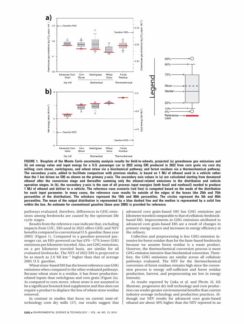
pathways evaluated, therefore, differences in GHG emis-sions among feedstocks are caused by the upstream lifecycle stages.

Results from the reference case indicate that, excludingimpacts from LUC, E85 used in 2022 offers GHG and NEVbenefits compared to conventional U.S. gasoline (base year2005) (Figure 1). Compared to a gasoline-powered pas-senger car, an E85-powered car has 43%-57% lower GHGemissions per kilometer traveled. Also, net GHG emissions,on a per kilometer traveled basis, are similar for allevaluated feedstocks. The NEV of 2022 E85 is projected tobe as much as 2.6 MJ km-1 higher than that of average2005 U.S. gasoline.

Wheat straw-based E85 has the lowest reference case GHGemissions when compared to the other evaluated pathways.Because wheat straw is a residue, it has fewer production-related inputs than switchgrass and corn grain (Figure 2a).As compared to corn stover, wheat straw is not assumed tobe a significant livestock feed supplement and thus does notrequire a product to displace the loss of wheat straw residueremoved.

In contrast to studies that focus on current state-of-technology corn dry mills (57), our results suggest that

advanced corn grain-based E85 has GHG emissions perkilometer traveled comparable to that of cellulosic feedstock-based E85. Improvements in GHG emissions attributed toadvanced corn grain-based E85 are a result of changes inprimary energy source and increases in energy efficiency atthe refinery.

Collection and preprocessing is less GHG-emission in-tensive for forest residue than for the farm-based feedstocksbecause we assume forest residue is a waste product.However, the thermochemical conversion process is moreGHG-emission intensive than biochemical conversion. There-fore, the GHG emissions are similar across all cellulosicpathways evaluated. The NEV for the thermochemicalconversion of forest residues remains high since the conver-sion process is energy self-sufficient and forest residueproduction, harvest, and preprocessing are low in energyintensity.

As results reported by Liska et al. and Plevin (6, 63)illustrate, progressive dry mill technology and corn produc-tion can render greater environmental benefits than currentindustry-average technology and production practices. Al-though our NEV results for advanced corn grain-basedethanol are about 30% higher than the NEV reported in an

FIGURE 1. Boxplots of the Monte Carlo uncertainty analysis results for field-to-wheels, projected (a) greenhouse gas emissions and(b) net energy value and input energy for a U.S. passenger car in 2022 using E85 produced in 2022 from corn grain via corn drymilling; corn stover, switchgrass, and wheat straw via a biochemical pathway; and forest residues via a thermochemical pathway.The secondary y-axis, added to facilitate comparison with previous studies, is based on 1 MJ of ethanol used in a vehicle ratherthan the 1 km driven on E85 as shown on the primary y-axis. The secondary axis values in (a) are calculated starting from denaturedethanol after the conversion stage and thereafter summing only the ethanol-related emissions in the distribution and vehicleoperation stages. In (b), the secondary y-axis is the sum of all process input energies (both fossil and nonfossil) needed to produce1 MJ of ethanol and deliver to a vehicle. The reference case scenario (red line) is computed based on the mode of the distributionfor each input parameter. In many cases, the reference case results lie outside of the edges of the boxes (the 25th and 75thpercentiles of the distribution). The whiskers represent the 10th and 90th percentiles. The circles represent the 5th and 95thpercentiles. The mean of the output distribution is represented by a blue dashed line and the median is represented by a solid linewithin the box. An estimate for conventional gasoline (base year 2005) is provided for reference.

5292 9 ENVIRONMENTAL SCIENCE & TECHNOLOGY / VOL. 44, NO. 13, 2010

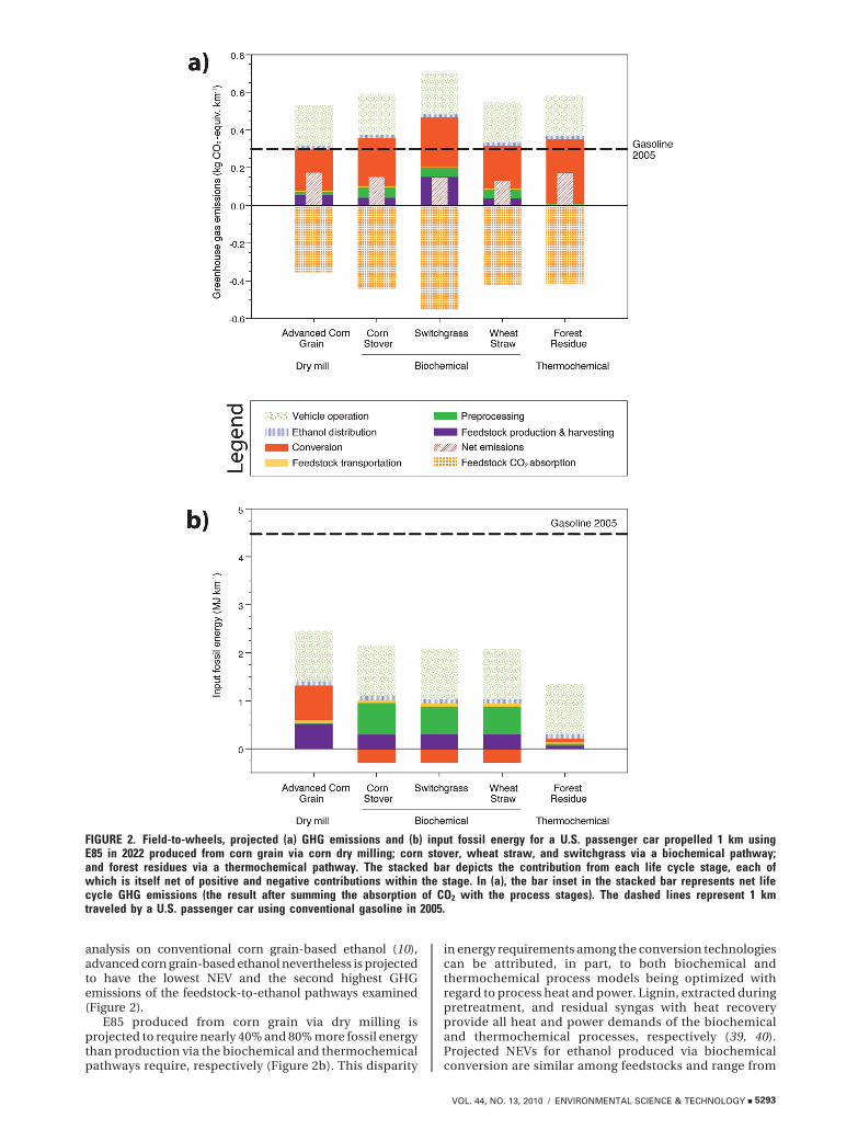
analysis on conventional corn grain-based ethanol (10),advanced corn grain-based ethanol nevertheless is projectedto have the lowest NEV and the second highest GHGemissions of the feedstock-to-ethanol pathways examined(Figure 2).

E85 produced from corn grain via dry milling isprojected to require nearly 40% and 80% more fossil energythan production via the biochemical and thermochemicalpathways require, respectively (Figure 2b). This disparity

in energy requirements among the conversion technologiescan be attributed, in part, to both biochemical andthermochemical process models being optimized withregard to process heat and power. Lignin, extracted duringpretreatment, and residual syngas with heat recoveryprovide all heat and power demands of the biochemicaland thermochemical processes, respectively (39, 40).Projected NEVs for ethanol produced via biochemicalconversion are similar among feedstocks and range from

FIGURE 2. Field-to-wheels, projected (a) GHG emissions and (b) input fossil energy for a U.S. passenger car propelled 1 km usingE85 in 2022 produced from corn grain via corn dry milling; corn stover, wheat straw, and switchgrass via a biochemical pathway;and forest residues via a thermochemical pathway. The stacked bar depicts the contribution from each life cycle stage, each ofwhich is itself net of positive and negative contributions within the stage. In (a), the bar inset in the stacked bar represents net lifecycle GHG emissions (the result after summing the absorption of CO2 with the process stages). The dashed lines represent 1 kmtraveled by a U.S. passenger car using conventional gasoline in 2005.

VOL. 44, NO. 13, 2010 / ENVIRONMENTAL SCIENCE & TECHNOLOGY 9 5293

1.0 to 1.1 MJ km-1 (Figures 1b and 2b). For those threefeedstocks, the majority of the fossil energy demand isattributed to the feedstock production and preprocessingstages (Figure 2b). Notably, preprocessing accounts fornearly 50% of the field-to-refinery gate fossil energyattributed to switchgrass-based ethanol (see Table S5).Preprocessing (e.g., drying and grinding) is energy intensiveyet necessary to ensure an efficient feedstock supplysystem. Improvements to energy efficiency of preprocess-ing are important to reducing the net GHG emissions andfossil energy demand attributed to ethanol produced viathe biochemical feedstock-to-ethanol pathways evaluated.

Fertilizer use dominates the GHG emissions from thefeedstock production phase for most evaluated feedstock-to-ethanol pathways (see Tables S4 and S5 for processcontribution details). Fertilization accounts for 13%-43% ofthe net fossil energy demand and 32%-56% of the net GHGemissions from the starch and herbaceous feedstocks. Muchof the GHG emissions and fossil energy demand of fertilizeris attributed to the production of inorganic nitrogen fertilizers.In contrast to dedicated crops, nitrogen fertilization for theagricultural residues is assumed to be applied at the rateneeded to replace nitrogen removed in the biomass. Switch-grass is assumed to be produced to maximize biomass yields;therefore, a nitrogen application rate of 10 kg N per Mg ofdesired biomass yield is assumed (24, 62). Considering thatnitrogen use efficiency for cereal crops is estimated to be33% (64) and that the application of nitrogen fertilizer hasa strong influence on the life cycle fossil energy input andGHG emissions, reduced fertilizer use and improved man-agement may offer viable and substantial GHG benefits toboth starch- and cellulosic-based ethanol.

E85 produced via thermochemical conversion of forestresidues is projected to have the highest NEV compared toall other E85 pathways evaluated. Because forest residues

are assumed to be a waste product, only chipping and loadingare attributed to forest residue-based E85 in the feedstockproduction and preprocessing stages. The allocation methodand type of timber harvesting operation assumed could bothhave significant implications for the overall life cycle impactsof E85 derived from forest residues. For instance, timberharvesting operations such as bole-only and cut-to-lengthresult in residues being left in dispersed piles throughout theforest (33), which would necessitate a separate harvestingoperation to collect said residues.

The corn dry mill and biochemical conversion processeshave significant GHG and NEV credits associated with theproduction of coproducts, which are assumed to displacefunctionally equivalent products in the marketplace. If thesecoproducts were to provide no value, then the GHG emissionswould be 20%-30% higher.

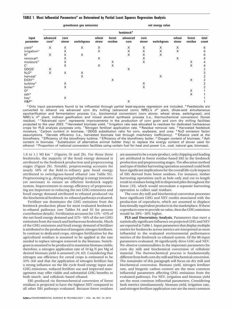
PLS and Uncertainty Analysis. Parameters that exert astatistically significant influence on projected GHG and NEVare reported in Table 1. Input parameters that display multipleentries for feedstocks across metrics are interpreted as mostinfluential to the evaluated environmental performancemetrics of the feedstock-to-ethanol system. Of the 86 inputparameters evaluated, 30 significantly drive GHG and NEV.We observe commonalities in the important parameters forcorn dry mill and biochemical conversion of cellulosicmaterial. The thermochemical process is fundamentallydifferent from both corn dry mill and biochemical conversion.The remainder of this paragraph will focus on dry mill andbiochemical conversion. Biomass yield, nitrogen fertilizerrate, and biogenic carbon content are the most commoninfluential parameters affecting GHG emissions from theevaluated pathways. For NEV, irrigation and biomass yieldare the most common influential parameters. Consideringboth metrics simultaneously, biomass yield, irrigation rate,and nitrogen fertilizer application rate are the most common

TABLE 1. Most Influential Parametersa as Determined by Partial Least Squares Regression Analysis

greenhouse gas emissions net energy value

feedstockb

inputparameter

advancedcornc

cornstover switchgrass

wheatstraw

forestresidue

advancedcorn

cornstover switchgrass

wheatstraw

forestresidue

totalcount

yieldd X X X X X X X X 8irrigatione X X X X X X 6Nf X X X X X X 6removalg X X X X 4moistureh X X X X 4Ci X X X X 4DDGSj X X 2N2Ok X X X 3harvestl X X 2EtOHm X X 2turbinen X X 2boilero X X 2Op X 1ashq X 1hayr X 1H&Ps X 1

a Only input parameters found to be influential through partial least-squares regression are included. b Feedstocks areconverted to ethanol via advanced corn dry milling (advanced corn); NREL’s nth plant, dilute-acid simultaneoussaccharification and fermentation process (i.e., biochemical conversion) (corn stover, wheat straw, switchgrass); andNREL’s nth plant, indirect gasification and mixed alcohol synthesis process (i.e., thermochemical conversion) (forestresidue). c “Advanced corn” represents improvements in the production of corn grain and corn dry milling facilitiesprojected to the year 2022. d Harvested biomass yield. e Irrigation rate was allocated to residues for dedicated herbaceouscrops for PLS analysis purposes only. f Nitrogen fertilizer application rate. g Residue removal rate. h Harvested feedstockmoisture. i Carbon content in biomass. j DDGS substitution ratio for corn, soybeans, and urea. k N2O emission factorassumptions. l Harvest efficiency (i.e., harvested biomass lost through machinery inefficiency). m Ethanol yield at thebiorefinery. n Efficiency of the biorefinery turbine. o Efficiency of the biorefinery boiler. p Oxygen content of biomass. q Ashcontent in biomass. r Substitution of alternative animal fodder (hay) to replace the energy content of stover used forethanol. s Proportion of national conversion facilities using certain fuel for heat and power (i.e., coal, natural gas, biomass).

5294 9 ENVIRONMENTAL SCIENCE & TECHNOLOGY / VOL. 44, NO. 13, 2010

influential parameters. This sensitivity analysis highlightsthe importance of the feedstock production phase to theGHG emissions and NEV of the evaluated ethanol productionsystems.

Results of the Monte Carlo uncertainty analysis arepresented in Figure 1. Despite any statistically significantdifferences in the mean values, given the large interquartileranges for most feedstocks, these differences (at most 0.04kg km-1 for GHG and 1.3 MJ km-1 for NEV) may notmanifest themselves in practice. Differences in NEV appearto cluster by conversion technology rather than byfeedstocks. The wide range of projected GHG emissionsand NEV suggests that even within a limited analytic scope(i.e., using attributional instead of consequential LCA),there is significant uncertainty in the estimates. Forinstance, switchgrass displays the widest variability inprojected GHG emissions and NEV among the evaluatedfeedstocks. Unlike the other feedstocks, switchgrass is notcurrently produced at a large scale and thus has moreuncertainty related to its production and harvest.

In this study, the reference case estimates tend to skewto one end of the projected frequency distribution (Figure1). Monte Carlo uncertainty analyses are sensitive to thePDF assumed. Scenarios that have GHG emissions the sameas or lower than the reference case often occur in the 25thpercentile of the distribution of results, and sometimes inthe 10th percentile. NEV results are similarly skewed. Theseresults are typically driven by skewed PDFs assumed forone or two of the most influential input parameters, whichare mostly assumed to be triangular. For example, thereference case switchgrass-E85 GHG emissions occurringbelow the 25th percentile of the projected range of GHGemissions is strongly influenced by the assumed valuesand PDF for the N2O emission factor, the biomass yield,and the application rate of nitrogen fertilizer. The IPCCN2O emission factor of 1.325% of all nitrogen-basedfertilizer applied is assumed for the reference case estimate,which is the mode of an assumed triangular distribution(65). A maximum of 4.00% (66) and a minimum of 0.40%is selected based on GREET (38). Holding all otherparameters constant, N2O alone accounts for 19% of thedeviation between the reference-case estimate of life cycleGHG emissions and the median of the frequency distribu-tion. An additional 53% of the deviation in GHG emissionsis accounted for by the biomass yield and the nitrogenfertilizer applied. As with the N2O emission factor, theyield and nitrogen fertilizer inputs are assumed to haveskewed triangular distributions based on expert interpre-tation (25, 67). Analogous to the value from the sensitivityanalysis, identifying the parameters that largely explainthose cases where the reference case scenario is found tobe extremely unlikely can help focus research and devel-opment of biofuel systems to (1) reduce uncertainty in theknowledge of and variability in key input parameterprobability distributions, and (2) improve key parametersto enhance the GHG emissions and NEV of the system.

Forest residue-based E85, in contrast to the other evalu-ated feedstock-to-ethanol pathways, has a median result closeto the reference case. This could be an artifact of modelinglimitations and assumptions. Although the projection thatfuture practice will resemble the present, with little im-provement, is based on expert elicitation, it is subject toconsiderable uncertainty, as commercial-scale collection anduse of forest residues does not currently exist. Furthermore,use of the product-purpose allocation method limits thenumber of input parameters tested in the uncertaintyanalysis. Finally, few influential input parameters to thispathway exhibit skewed PFDs.

Although results from the uncertainty analysis suggestthe reference case is, in many instances, outside the middle

50%-80% of the distribution, the median outcome for bothGHG emissions (not considering LUC) and NEV across allfeedstock-to-ethanol pathways evaluated is still an im-provement over conventional U.S. gasoline in 2005. In thecontext of the reference case and uncertainty resultspresented in this study, the reference case scenario appearsto represent an optimistic case in which most keyparameters are optimized in concert. In reality, however,all key parameters may not be optimized at any one time.This insight underscores the need to ensure the achieve-ment of optimal performance for key parameters involvedin feedstock production, harvest, and conversion to ethanolthrough targeted research and industrial experience.

AcknowledgmentsAuthors D.D.H. and D.I. contributed equally to this work.Funding for this project was provided by the U.S. Depart-ment of Energy’s Office of the Biomass Program (DE-AC36-08-GO28308). Feedback and contributions from the fol-lowing people are greatly appreciated: Brian Bush, HelenaChum, Joyce Cooper, Nathan Fields, Thomas Foust, AlisonGoss Eng, Zia Haq, Sara Havig, Jacob Jacobson, LeonardJohnson, Lise Laurin, Andy McAloon, Laurel McEwen,Leslie Miller, Elaine Oneil, Bob Reynolds, Robert Rummer,Heather Wakeley, Bob Wallace, Michael Wang, DwayneWestfall, Christopher Wright, May Wu, Winnie Yee, andYimin Zhang.

Supporting Information AvailableDetailed information describing the construction of thelife cycle assessment models for each feedstock-to-ethanolpathway, as well as additional results. This material isavailable free of charge via the Internet at http://pub-s.acs.org.

Literature Cited(1) Renewable Fuels Association Statistics: Historic U.S. Fuel Ethanol

Production. www.ethanolrfa.org/pages/statistics/ (accessed April12, 2010).

(2) Energy Independence and Security Act of 2007. Public Law 110-140, 2007; Vol. 121.

(3) Pimentel, D.; Patzek, T. Ethanol Production Using Corn,Switchgrass, and Wood; Biodiesel Production Using Soybeanand Sunflower. Nat. Resour. Res. 2005, 14 (1), 65–76.

(4) Patzek, T. W.; Pimentel, D. Thermodynamics of energy produc-tion from biomass. Crit. Rev. Plant Sci. 2005, 24 (5-6), 327–364.

(5) Wang, M.; Wu, M.; Hong, H. Life-cycle energy and greenhousegas emission impacts of different corn ethanol plant types.Environ. Res. Lett. 2007, 2, 024001.

(6) Liska, A. J.; Yang, H. S.; Bremer, V. R.; Klopfenstein, T. J.; Walters,D. T.; Erickson, G. E.; Cassman, K. G. Improvements in LifeCycle Energy Efficiency and Greenhouse Gas Emissions of Corn-Ethanol. J. Ind. Ecol. 2009, 13 (1), 58–74.

(7) Shapouri, H.; Duffield, J. A.; Wang, M. The energy balance ofcorn ethanol revisited. Trans. ASAE 2003, 46 (4), 959–968.

(8) Graboski, M. S. Fossil Energy Use in the Manufacture of CornEthanol; Colorado School of Mines: Golden, CO, 2002.

(9) De Oliveira, M. E. D.; Vaughan, B. E.; Rykiel, E. J., Jr. Ethanolas fuels: Energy, carbon dioxide balances, and ecologicalfootprint. Bioscience 2005, 55 (7), 593–602.

(10) Farrell, A. E.; Plevin, R. J.; Turner, B. T.; Jones, A. D.; O’Hare, M.;Kammen, D. M. Energy returns on ethanol production -Response. Science 2006, 312 (5781), 1747–1748.

(11) Schmer, M. R.; Vogel, K. P.; Mitchell, R. B.; Perrin, R. K. NetEnergy of Cellulosic Ethanol from Switchgrass. Proc. Nat. Acad.Sci., U.S.A. 2008, 105 (2), 464–469.

(12) Sheehan, J.; Aden, A.; Paustian, K.; Killian, K.; Brenner, J.; Walsh,M.; Nelson, R. Energy and Environmental Aspects of Using CornStover for Fuel Ethanol. J. Ind. Ecol. 2004, 7 (3-4), 117–146.

(13) SimaPro, v.7.1; Product Ecology Consultants: Amersfoort, theNetherlands, 2008.

(14) Ecoinvent, v.2.0; Swiss Center for Life Cycle Inventories:Duebendorf, Switzerland, 2007.

(15) U.S. Life-Cycle Inventory, v. 1.6.0; National Renewable EnergyLaboratory: Golden, CO, 2008.

VOL. 44, NO. 13, 2010 / ENVIRONMENTAL SCIENCE & TECHNOLOGY 9 5295

(16) International Organization for Standardization. Environmentalmanagement -- Life Cycle Assessment -- Principles and Frame-work; ISO 14040:2006; International Organization for Stan-dardization: Geneva, Switzerland, 2006.

(17) International Organization for Standardization. Environmentalmanagement -- Life Cycle Assessment -- Requirements andGuidelines; ISO 14044:2006; International Organization forStandardization: Geneva, Switzerland, 2006.

(18) Perlack, R. D.; Wright, L. L.; Turhollow, A. F.; Graham, R. L.;Stokes, B. J.; Erbach, D. C. Biomass as Feedstock for a Bioenergyand Bioproducts Industry: The Technical Feasibility of a Billion-Ton Annual Supply; DOE/GO-102005-2135, ORNL/TM-2005/66; United States Department of Energy, Oak Ridge NationalLaboratory: Oak Ridge, TN, 2005.

(19) EERE. Handbook for Handling, Storing, and Dispensing E85;DOE: Washington, DC, 2008; p 54.

(20) Wang, M.; Huo, H.; Arora, S. Methods of dealing with co-productsof biofuels in life-cycle analysis and consequent results withinthe U.S. context. Energy Policy 2010; doi:10.1016/j.en-pol.2010.03.052.

(21) Searchinger, T.; Heimlich, R.; Houghton, R. A.; Dong, F.; Elobeid,A.; Fabiosa, J.; Tokgoz, S.; Hayes, D.; Yu, T.-H. Use of U.S.Croplands for Biofuels Increases Greenhouse Gases ThroughEmissions From Land-Use Change. Science 2008, 319 (5867),1238–1240.

(22) Fargione, J.; Hill, J.; Tilman, D.; Polasky, S.; Hawthorne, P. LandClearing and Biofuel Carbon Debt. Science 2008, 319 (5867),1235–1238.

(23) USDA-NASS National Agricultural Statistics Service Quick Stats.http://www.nass.usda.gov/QuickStats (December 15, 2008).

(24) Perrin, R. K.; Vogel, K. P.; Schmer, M. R.; Mitchell, R. B. Farm-Scale Production Cost of Switchgrass for Biomass. BioEnergyRes. 2008, 1 (1), 91–97.

(25) Sokhansanj, S.; Mani, S.; Turhollow, A.; Kumar, A.; Bransby, D.;Lynd, L.; Laser, M. Large-scale production, harvest and logisticsof switchgrass (Panicum virgatum L.) -current technology andenvisioning a mature technology. Biofuels Bioprod. Biorefin.2009, 3 (2), 124–141.

(26) Southgate, D.; Graham, D. H.; Tweeten, L. The World FoodEconomy., 1st ed.; Blackwell: Malden, MA, 2007; p 401.

(27) Graham, R. L.; Nelson, R.; Sheehan, J.; Perlack, R. D.; Wright,L. L. Current and potential US corn stover supplies. Agron. J.2007, 99 (1), 1–11.

(28) Edwards, W. Estimating a Value for Corn Stover; File A1-70;Iowa State University- Extension: Ames, IA, December 2007.

(29) Hess, J. R.; Kenny, K. L.; Ovard, L. P.; Searcy, E. M.; Wright,C. T. Uniform-format solid feedstock supply system; INL/EXT-08-14752; Idaho National Laboratory: Idaho Falls, ID, April2009.

(30) Smith, W. B.; Miles, P. D.; Vissage, J. S.; Pugh, S. A. Forest Resourcesof the United States, 2002; NC-241; USFS: St. Paul, MN, 2004;p 146.

(31) Jacobson, J. J. Personal communication. Idaho National Labo-ratory: 2008.

(32) Yu, T.-H.; Hart, C. E. The 2006/07 Iowa Grain and Biofuel FlowStudy: A Survey Report; 08-SR 102; Center for Agricultural andRural Development, Iowa State University: Ames, Iowa, October2008.

(33) Leinonen, A. Harvesting technology of forest residues for fuel inthe USA and Finland; Espoo 2004 VTT Tiedotteita-ResearchNotes 2229; VTT Processes: Finland, 2004.

(34) Pan, F.; Han, H.-S.; Johnson, L. R.; Elliot, W. J. Net energy outputfrom harvesting small-diameter trees using a mechanizedsystem. Forest Prod. J. 2008, 58 (1/2), 25–30.

(35) Wakeley, H. L.; Hendrickson, C. T.; Griffin, W. M.; Matthews,H. S. Economic and Environmental Transporation Effects ofLarge-Scale Ethanol Production and Distribution in the UnitedStates. Environ. Sci. Technol. 2009, 43 (7), 2228–2233.

(36) Denicoff, M. R. Ethanol Transportation Backgrounder: Expansionof U.S. Corn-based Ethanol from the Agricultural TransportationPerspective; United States Department of Agriculture: Wash-ington, DC, September 2007; pp 1-29.

(37) Shapouri, H.; Duffield, J. A.; Wang, M. The Energy Balance ofCorn Ethanol: An Update; Agricultural Economic Report No.814; United States Department of Agriculture, Office of the ChiefEconomist, Office of Energy Policy and New Uses: Washington,DC, July 2002.

(38) The Greenhouse Gases, Regulated Emissions, and Energy Use inTransportation (GREET) Model, v1.8c; Argonne National Labo-ratory: Argonne, IL, 2008.

(39) Aden, A.; Ruth, M.; Ibsen, K.; Jechura, J.; Neeves, K.; Sheehan,J.; Wallace, B. Lignocellulosic Biomass to Ethanol Process

Design and Economics Utilizing Co-Current Dilute AcidPrehydrolysis and Enzymatic Hydrolysis for Corn Stover; TP-510-32438; National Renewable Energy Laboratory: Golden,CO, June 2002.

(40) Phillips, S.; Aden, A.; Jechura, J.; Dayton, D.; Eggeman, T.Thermochemical Ethanol via Indirect Gasification and MixedAlcohol Synthesis of Lignocellulosic Biomass; TP-510-41168;National Renewable Energy Laboratory: Golden, CO, April2007.

(41) Lee, D.; Owens, V. N.; Boe, A.; Jeranyama, P. Composition ofHerbaceous Biomass Feedstocks; South Dakota State University:Brookings, SD, June 2007.

(42) McAloon, A.; Taylor, F.; Yee, W.; Ibsen, K.; Wooley, R. Determiningthe Cost of Producing Ethanol from Corn Starch and Lignocel-lulosic Feedstocks; NREL/TP-580-28893; National RenewableEnergy Laboratory: Golden, CO, October 2000.

(43) Mueller, S. An analysis of the projected energy use of future drymill corn ethanol plants (2010-2030); Energy Resources CenterReport; University of Illinois at Chicago: Chicago, IL, October10, 2007.

(44) Nielsen, P. H.; Oxenboll, K. M.; Wenzel, H. Cradle-to-gateenvironmental assessment of enzyme products producedindustrially in Denmark by Novozymes A/S. Int. J. Life CycleAssess. 2007, 12 (6), 432–438.

(45) Oxenboll, K. M., Personal communication. Novozymes, 2008.(46) Jungbluth, N.; Dinkel, F.; Doka, G.; Chudacoft, M.; Dauriat, A.;

Gnansounou, E.; Sutter, J.; Speilmann, M.; Kljun, N.; Keller, M.;Schleiss, K. Life Cycle Inventories of Bioenergy: Data v2.0;ecoinvent report No. 17; Swiss Centre for Life Cycle Inventories:Dubendorf, Switzerland, December 2007.

(47) Arora, S.; Wu, M.; Wang, M. Update of Distillers GrainsDisplacement Ratios for Corn Ethanol Life-Cycle Analysis;Argonne National Laboratory: Argonne, IL, 2008; pp 1-15.

(48) Nemecek, T.; Kagi, T. Life Cycle Inventories of AgriculturalProduction Systems Data 2.0; Swiss Centre for Life CycleInventories: Zurich and Dubendorf, Switzerland, December,2007.

(49) EPA. AP-42 Compilation of Air Pollutant Emissions Factors; U.S.Environmental Protection Agency: Washington, DC, August2007.

(50) National Renewable Energy Laboratory Biorefinery AnalysisProcess Models. http://www.nrel.gov/extranet/biorefinery/as-pen_models/ (accessed April 23, 2010).

(51) Reynolds, R. E. Ethanol’s Potential Contribution to U.S. Trans-portation Fuel Pool; Downstream Alternatives Inc.: South Bend,IN, December 31, 2006.

(52) Reynolds, R. Personal Communication. Downstream AlternativesInc.: South Bend, IN, 2008.

(53) Morrow, W. R.; Griffin, W. M.; Matthews, H. S. Modelingswitchgrass derived cellulosic ethanol distribution in the UnitedStates. Environ. Sci. Technol. 2006, 40 (9), 2877–2886.

(54) Farrington, R. Invited Testimony for the U.S. Senate Committeeon Finance, Prepared Statement of Dr. Robert Farrington,Manager & Principal Researcher, Advanced Vehicle SystemsGroup, National Renewable Energy Laboratory, Golden, CO,April 19, 2007. In Committee, U. S. S. F., Ed. Washington, DC,2007.

(55) Charpentier, A. D.; Bergerson, J. A.; MacLean, H. Understandingthe Canadian oil sands industry’s greenhouse gas emissions.Env. Res. Lett. 2009, 4, 014005.

(56) Forster, P.; Ramaswamy, V.; Artaxo, P.; Berntsen, T.; Betts, R.;Fahey, D. W.; Haywood, J.; Lean, J.; Lowe, D. C.; Myhre, G.;Nganga, J.; Prinn, R.; Raga, G.; Schulz, M.; Van Dorland, R.,Changes in Atmospheric Constituents and in RadiativeForcing. In Climate Change 2007: The Physical Science Basis.Contribution of Working Group I to the Fourth AssessmentReport of the Intergovernmental Panel on Climate Change;Solomon, S.; Qin, D.; Manning, M.; Chen, Z.; Marquis, M.; Averyt,K. B.; Tignor, M.; Miller, H. L., Eds.; Cambridge University Press:Cambridge, UK and New York, 2007; pp 129-234.

(57) Farrell, A. E.; Plevin, R. J.; Turner, B. T.; Jones, A. D.; O’Hare, M.;Kammen, D. M. Ethanol can contribute to energy and envi-ronmental goals. Science 2006, 311 (5760), 506–508.

(58) Brereton, R. Applied Chemometrics for Scientists; John Wiley &Sons, Ltd.: Chichester, West Sussex, UK, 2007.

(59) Martens, H.; Martens, M. Analysis of designed experiments bystabilised PLS Regression and jack-knifing. Food Qual. Pref. 2000,11 (1-2), 5–16.

(60) Esbensen, K. H. Multivariate Data Analysis in Practice, 5th ed.;Camo Process AS: Oslo, Norway, 2002.

(61) The Unscrambler 9.8; CAMO Software AS: Oslo, Norway,2008.

5296 9 ENVIRONMENTAL SCIENCE & TECHNOLOGY / VOL. 44, NO. 13, 2010

(62) Vogel, K. P.; Brejda, J. J.; Walters, D. T.; Buxton, D. R. SwitchgrassBiomass Production in the Midwest USA: Harvest and NitrogenManagement. Agron. J. 2002, 94, 413–420.

(63) Plevin, R. J. Modeling Corn Ethanol and Climate. A CriticalComparison of the BESS and GREET Models. J. Ind. Ecol. 2009,13 (4), 495–507.

(64) Raun, W. R.; Johnson, G. V. Improving Nitrogen Use Efficiencyfor Cereal Production. Agron. J. 1999, 91, 357–363.

(65) Klein, C. D.; Novoa, R. S. A.; Ogle, S.; Smith, K. A.; Rochette, P.;Wirth, T. C.; McConkey, B. G.; Mosier, A.; Rypdal, K.; Walsh, M.;Williams, S. A., Chapter 11: N2O Emissions from Managed Soils,and CO2 Emissions from Lime and Urea Application. In 2006

IPCC Guidelines for National Greenhouse Gas Inventories, Vol.4: Agriculture, Forestry, and Other Land Use; Eggleston, S.;Buendia, L.; Miwa, K.; Ngara, T.; Tanabe, K., Eds.; IGES: Japan,2006.

(66) Crutzen, P. J.; Mosier, A. R.; Smith, K. A.; Winiwarter, W. N2Orelease from agro-biofuel production negates global warmingreduction by replacing fossil fuels. Atmos. Chem. Phys. 2008, 8(2), 389–395.

(67) Perrin, R. K.; Williams, B. The Outlook for Switchgrass as anEnergy Crop. Cornhusker Economics 2008, 2 pp.

ES100186H

VOL. 44, NO. 13, 2010 / ENVIRONMENTAL SCIENCE & TECHNOLOGY 9 5297