Embed Size (px)
Citation preview
Life Principle-Based Reserves Under VM-20
A P u b l i c P o l i c y P r A c t i c e N o t e
ExposurE DraftFebruary 2014
American Academy of ActuariesLife Principle-Based Approach Practice Note Work Group
A PUBLIC POLICY PRACTICE NOTE
Practice Note on Life Principle-Based Reserves Under VM-20
February 2014
Developed by the Life Principle-Based Approach Practice Note Work Group of the American Academy of Actuaries
The American Academy of Actuaries is a professional association with over 17,500 members, whose mission is to assist public policymakers by providing leadership,
objective expertise, and actuarial advice on risk and financial security issues. The Academy also sets qualification, practice, and professionalism standards
for actuaries in the United States.
VM-20 Practice Note
© 2014 American Academy of Actuaries. All rights reserved.
This practice note is not a promulgation of the Actuarial Standards Board, is not an actuarial standard of practice, is not binding upon any actuary and is not a definitive statement as to what constitutes generally accepted practice in the area under discussion. Events occurring subsequent to this publication of the practice note may make the practices described in this practice note irrelevant or obsolete.
Life Principle-Based Approach Practice Note Work Group
Todd H. Erkis, FSA, MAAA, CERA, Chairperson
Nadeem Chowdhury, FSA, MAAA Shane Ewen, FIAA, FSA, MAAA Christopher Fioritto, FSA, MAAA Alice Fontaine, FSA, FCIA, MAAA, FCA R. Dale Hall, FSA, MAAA, CERA Manuel V. Hidalgo, FSA, MAAA, CFA Norman E. Hill, FSA, MAAA Pamela Hutchins, FSA, MAAA Sheetal Kaura, ASA, MAAA, CERA Josh Kendrach, FSA Kristin J. Kuhn, FSA, MAAA Veltcho Natchev, FSA, MAAA
David E. Neve, FSA, MAAA, CERA Randall O’Connor, FSA, MAAA Arthur V. Panighetti, FSA, MAAA Craig W. Reynolds, FSA, MAAA Roland Rose, FSA, MAAA Karen K. Rudolph, FSA, MAAA Prabhdeep Singh, FSA, MAAA, CERA David V. Smith, FSA, MAAA, CERA Lloyd Spencer, FSA, MAAA, CERA Dale Ward, FSA Amanda E. Young, FSA, CPA, MAAA
1850 M Street N.W., Suite 300 Washington, D.C. 20036-5805
TABLE OF CONTENTS
Summary of VM-20 ....................................................................................................1
1. Details on Products Covered ..................................................................................3
2. Available Information on Common Practice ......................................................5
3. VM-20 Calculation .................................................................................................7
4. VM-20 Calculation Overview – Part A. Net Premium Reserve (NPR) ...........14
5: VM-20 Calculation Overview – Part B. Deterministic Reserve ......................23
6: VM-20 Calculation Overview – Part C. Stochastic Reserve ...........................25
7. Stochastic Exclusion Test .....................................................................................29
8: Deterministic Reserve Exclusion Test ................................................................34
9. Difference from Cash Flow Testing – Scenario Reserve Calculation ..............37
10. Considerations When Performing Work on Other Than the Valuation Date40
11. Detail on Starting Assets and Asset Modeling .................................................43
12. Details on Scenarios / Scenario Generators / Economic Assumptions ...........58
13. Setting Prudent Estimate and Anticipated Experience Assumptions ............63
14. Setting Margins ...................................................................................................67
15. Setting Mortality Assumptions ..........................................................................71
16. Setting Premium Assumptions ..........................................................................80
17. Setting Policyholder Behavior Assumptions Other than Premiums ..............82
18. Setting Expense Assumptions ............................................................................86
19. Setting Non-Guaranteed Element Assumptions ..............................................89
20. Treatment of Reinsurance .................................................................................92
21. Treatment of Hedging / Derivative Programs ..................................................97
American Academy of Actuaries www.actuary.org 1
INTRODUCTION This practice note covers principle-based life insurance reserve practices for life insurance. Since the principle-based approach for life reserves is new, this practice note was not developed from a survey of current actuarial practices. The practices here represent the views of actuaries in industry, consulting, and public accounting firms that have been involved in the development of the proposed life reserving standards. The purpose of the practice note is to assist actuaries with the implementation of principle-based life reserves adopted by the NAIC as detailed in the Requirements for Principle-Based Reserves for Life Products – VM-20 dated December 2, 2012, describing the proposed requirements for calculating minimum valuation standard statutory reserves (“VM-20”) for life insurance products. The final requirements will be effective when they become law after being approved by the state legislatures and may differ from this version. It is expected that actuarial practice for determining principle-based statutory reserves for life insurance products will emerge over time. As this practice note is an expectation of what actuarial practice will emerge from the new standards prior to the effective date, it is likely that additional actuarial practice will be developed that are not contained in this practice note. The goal of this practice note was two-fold: to assist actuaries who are implementing VM-20 with the understanding of what the requirements are and to provide industry practice. The work group attempted to meet both goals as well as it could. Additions and revisions to this practice note will likely be needed in the future as practices are further developed and issues that are not anticipated below are addressed.
American Academy of Actuaries www.actuary.org 2
American Academy of Actuaries www.actuary.org 3
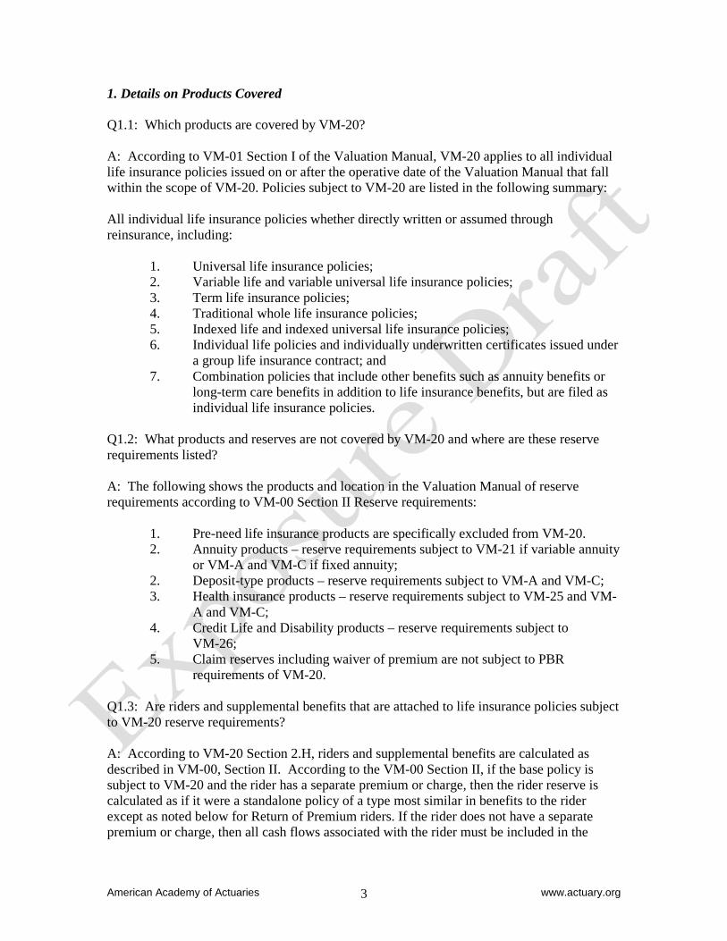
1. Details on Products Covered Q1.1: Which products are covered by VM-20? A: According to VM-01 Section I of the Valuation Manual, VM-20 applies to all individual life insurance policies issued on or after the operative date of the Valuation Manual that fall within the scope of VM-20. Policies subject to VM-20 are listed in the following summary: All individual life insurance policies whether directly written or assumed through reinsurance, including:
1. Universal life insurance policies; 2. Variable life and variable universal life insurance policies; 3. Term life insurance policies; 4. Traditional whole life insurance policies; 5. Indexed life and indexed universal life insurance policies; 6. Individual life policies and individually underwritten certificates issued under
a group life insurance contract; and 7. Combination policies that include other benefits such as annuity benefits or
long-term care benefits in addition to life insurance benefits, but are filed as individual life insurance policies.
Q1.2: What products and reserves are not covered by VM-20 and where are these reserve requirements listed? A: The following shows the products and location in the Valuation Manual of reserve requirements according to VM-00 Section II Reserve requirements:
1. Pre-need life insurance products are specifically excluded from VM-20. 2. Annuity products – reserve requirements subject to VM-21 if variable annuity
or VM-A and VM-C if fixed annuity; 2. Deposit-type products – reserve requirements subject to VM-A and VM-C; 3. Health insurance products – reserve requirements subject to VM-25 and VM-
A and VM-C; 4. Credit Life and Disability products – reserve requirements subject to
VM-26; 5. Claim reserves including waiver of premium are not subject to PBR
requirements of VM-20.
Q1.3: Are riders and supplemental benefits that are attached to life insurance policies subject to VM-20 reserve requirements? A: According to VM-20 Section 2.H, riders and supplemental benefits are calculated as described in VM-00, Section II. According to the VM-00 Section II, if the base policy is subject to VM-20 and the rider has a separate premium or charge, then the rider reserve is calculated as if it were a standalone policy of a type most similar in benefits to the rider except as noted below for Return of Premium riders. If the rider does not have a separate premium or charge, then all cash flows associated with the rider must be included in the
American Academy of Actuaries www.actuary.org 4
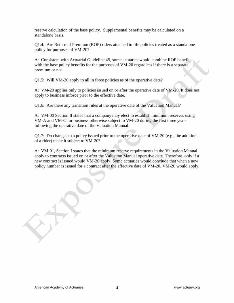
reserve calculation of the base policy. Supplemental benefits may be calculated on a standalone basis. Q1.4: Are Return of Premium (ROP) riders attached to life policies treated as a standalone policy for purposes of VM-20? A: Consistent with Actuarial Guideline 45, some actuaries would combine ROP benefits with the base policy benefits for the purposes of VM-20 regardless if there is a separate premium or not. Q1.5: Will VM-20 apply to all in force policies as of the operative date? A: VM-20 applies only to policies issued on or after the operative date of VM-20. It does not apply to business inforce prior to the effective date. Q1.6: Are there any transition rules at the operative date of the Valuation Manual? A: VM-00 Section II states that a company may elect to establish minimum reserves using VM-A and VM-C for business otherwise subject to VM-20 during the first three years following the operative date of the Valuation Manual. Q1.7: Do changes to a policy issued prior to the operative date of VM-20 (e.g., the addition of a rider) make it subject to VM-20? A: VM-01, Section I states that the minimum reserve requirements in the Valuation Manual apply to contracts issued on or after the Valuation Manual operative date. Therefore, only if a new contract is issued would VM-20 apply. Some actuaries would conclude that when a new policy number is issued for a contract after the effective date of VM-20, VM-20 would apply.
American Academy of Actuaries www.actuary.org 5
2. Available Information on Common Practice Q2.1: Which Actuarial Standards of Practice (ASOPs) would apply to the actuary when performing the tasks in conjunction with determining reserves under VM-20? A: While each actuary is ultimately responsible for determining which ASOPs are applicable to a specific task, the following ASOPs, as of the date of this practice note, are among those the actuary may wish to consider: No. 1 Introductory Actuarial Standard of Practice No. 2 Nonguaranteed Charges or Benefits for Life Insurance Policies and Annuity
Contracts. No. 7 Analysis of Life, Health, or Property/Casualty Insurer Cash Flows No. 11 Treatment of Reinsurance Transactions Involving Life or Health Insurance 1 No. 12 Risk Classification (for All Practice Areas) No. 15 Dividends for Individual Participating Life Insurance, Annuities, and Disability
Insurance No. 22 Statements of Opinion Based on Asset Adequacy Analysis by Actuaries for Life and
Health Insurers No. 23 Data Quality No. 38 Using Models Outside the Actuary’s Area of Expertise (Property and Casualty) No. 41 Actuarial Communications The Actuarial Standards Board is developing a new ASOP, Standards for Principle-Based Reserves for Life Products that the actuary likely will wish to also consider. Q2.2: Are there other practice notes that cover topics relevant to principle-based reserve calculations as described in the Valuation Manual? A: The Asset Adequacy Analysis Practice Note and the Credibility Practice Note may contain relevant information for actuaries performing PBA reserve calculations. These practice notes can be found at the American Academy of Actuaries web site at www.actuary.org. Q2.3: What are the qualification standards applicable to actuaries performing VM-20 calculations? A: As VM-20 does not modify the Actuarial Opinion and Memorandum Regulation (AOMR); the applicable standards are still defined by Section 5.B of that regulation. This includes satisfying basic education, experience and continuing education requirements. Section 5.B.2 of the AOMR requires the actuary to be qualified to sign statements of actuarial opinion for life and health insurance company annual statements in accordance with the Qualification Standards for Actuaries Issuing Statements of Actuarial Opinion in the United States promulgated by the American Academy of Actuaries which can be found at ://www.actuary.org/qualstandards/qual.pdf Q2.4: Are there practices in other countries that an actuary can review for reference?
American Academy of Actuaries www.actuary.org 6
A: Published papers on principle-based reserve calculations in other countries may provide useful information. It should be noted that acceptable practice in other countries may not be viewed as a safe harbor for principle-based calculations in the United States. U.S. actuaries using other countries’ papers as a guide should make their own independent decision as to whether the techniques described in the papers are appropriate for their situation under principle-based methods. The Canadian Institute of Actuaries has Valuation Technique Papers (VTP) and educational notes that U.S. actuaries may wish to consider in order to better understand how Canadian actuaries calculate reserves. There are some similarities between U.S. principle-based reserves and Canadian valuation techniques and a review of the specific Canadian material may be helpful to identify specific issues that a U.S. actuary might want to consider in calculating principle-based reserves. For Canadian documentation please see the Canadian Institute of Actuaries website at www.actuaries.ca.
American Academy of Actuaries www.actuary.org 7
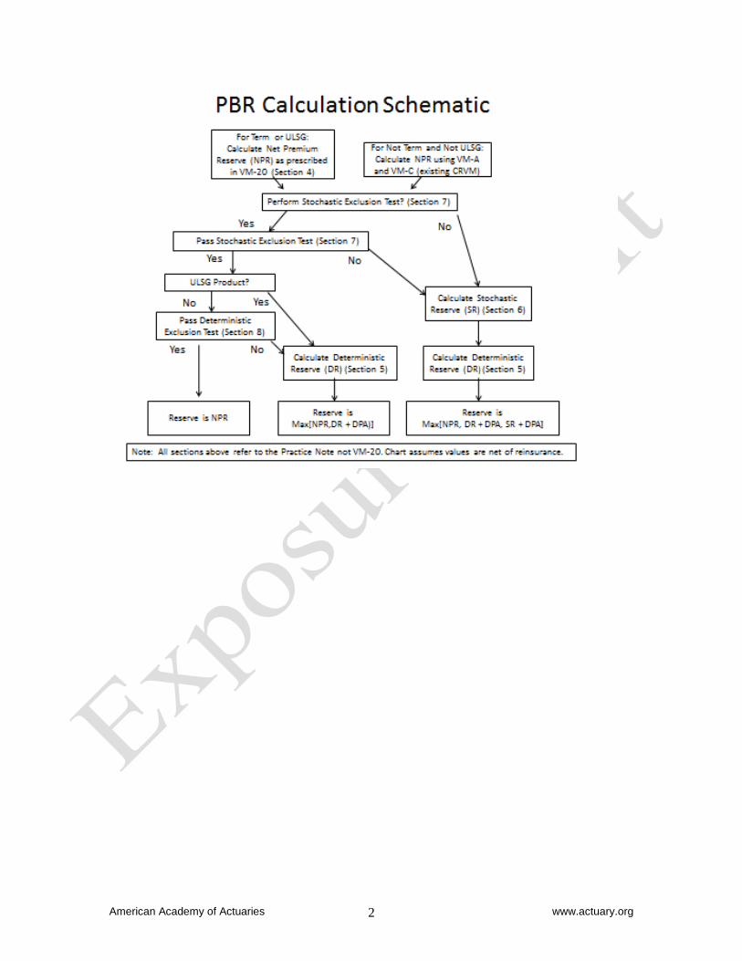
3. VM-20 Calculation Q3.1: VM-20 describes three components of the minimum reserve: the Net Premium Reserve, the Deterministic Reserve, and the Stochastic Reserve. Is the company required to calculate all three components for all policies? A: The Net Premium Reserve is required to be calculated for all policies subject to VM-20. The company may elect to perform exclusion tests that if passed, exempt some groups of policies from the Deterministic Reserve and the Stochastic Reserve. These exclusion tests are optional, and a company can decide to calculate all three components for all policies. Later sections of this practice note provide detail for each of the three components that go into the calculation of the minimum reserve: the Net Premium Reserve, the Deterministic Reserve, and the Stochastic Reserve. Q3.2: What is the minimum reserve for all policies as required by VM-20? A: Section 2.A of VM-20 states that the minimum reserve for all policies subject to VM-20 is determined as the aggregate Net Premium Reserve for all policies plus the excess, if any, of the greater of the Deterministic Reserve for all policies and the Stochastic Reserve for all policies over the difference between the aggregate Net Premium Reserve and any deferred premium asset held on account of those policies. All three reserve components are net of any credit for reinsurance ceded for those policies. In mathematical terms, this could be represented as: Minimum Reserve = AggNPR + Max(0, (Max(DR, SR) – (AggNPR – DPA))) Where AggNPR = Aggregate Net Premium Reserve DR = Deterministic Reserve SR = Stochastic Reserve DPA = Deferred Premium Asset Another way of expressing the minimum reserve that might be simpler for some people (and is also shown in the flowchart above in the Summary section) is the greatest of three quantities:
1) Aggregate Net Premium Reserve 2) Deterministic Reserve + Deferred Premium Asset 3) Stochastic Reserve + Deferred Premium Asset
The adjustment for the Deferred Premium Asset is used to gross up the SR and the DR for the purpose of comparing the SR and the DR to the NPR. The NPR may have an associated Deferred Premium Asset, and if so, it will end up on the balance sheet as an asset. When the SR or the DR is higher than the NPR less the DPA, adding the DPA to the DR or SR results
American Academy of Actuaries www.actuary.org 8
in the net impact on the balance sheet being exactly equal to the DR or SR (i.e., net of the DPA on the asset side of the balance sheet). If the company makes use of the exclusion tests, then for policies that pass both the Stochastic Exclusion Test and the Deterministic Exclusion Test, the minimum reserve for that group of policies is the aggregate Net Premium Reserve for those policies. For policies that pass the Stochastic Exclusion Test but not the Deterministic Exclusion Test, the minimum reserve equals (using wording from VM-20 in Section 2.A.1): the aggregate Net Premium Reserve plus the excess, if any of the Deterministic Reserve over the difference between the aggregate Net Premium Reserve for those policies and any deferred premium asset held on account of those policies. Another way to show this would be that the minimum reserve is the greatest of:
1) Aggregate Net Premium Reserve, or 2) Deterministic Reserve + Deferred Premium Asset
For policies that fail the Stochastic Exclusion Test and for policies not subjected to any exclusion tests, the minimum reserve equals (Section 2.A.3): the aggregate Net Premium Reserve plus the excess, if any of the greater of the Deterministic Reserve and the Stochastic Reserve over the difference between the aggregate Net Premium Reserve for those policies and any deferred premium asset held on account of those policies. The minimum reserve is the greater of:
1) Aggregate Net Premium Reserve, or 2) Deterministic Reserve + Deferred Premium Asset, or 3) Stochastic Reserve + Deferred Premium Asset
Q3.3: Why is the Deferred Premium Asset added to the Deterministic and Stochastic Reserve in the comparison above? A: Because two of the components of the comparison (the Deterministic Reserve and Stochastic Reserve) are calculated as of the reporting date and the Net Premium Reserve is as of the policy anniversary date so per statutory accounting rules an adjustment to the Net Premium Reserve is required to put all of the values on the same basis. Q3.4: Should due premiums be included along with deferred premiums when determining the Deferred Premium Adjustment in the minimum reserve calculation in Section 2 of VM-20? A: Although the version of VM-20 referenced in this practice note is silent on how due premiums are to be handled, some actuaries will treat due premiums similarly to deferred premiums when determining the adjustment for DPA in Section 2, since most actuaries will include due premiums in the expected future cash flows when calculating the Deterministic Reserve and Stochastic Reserve. This approach reduces the resulting DR and SR amounts compared to the reserve amounts that would be calculated had there been no due premiums in the cash flows. So in this case, some actuaries will find it appropriate to add due premiums to the DR and SR when making the comparison to the NPR. Other actuaries may not include
American Academy of Actuaries www.actuary.org 9
due premiums in future cash flows. In this case, those actuaries would not include due premiums in the DPA adjustment when making the comparison to the NPR. Q3.5: How would actuaries approach the calculation of the minimum reserve requirement under VM-20? A: One approach for completing the calculation is outlined below. Other approaches are possible. Refer to VM-20 for specific details.
1. Determine policies in scope of the VM-20 requirements.
2. Determine the model segments for all policies in scope of the requirements. Per the definition of Model Segment in Section 7A, this determination will generally align with the company’s asset segmentation plan, investment strategies or approach used to allocate investment income for statutory purposes. It should be noted that a model segment could be an entire block of business.
3. Select the amount of starting assets for the each model segment, and allocate existing assets to each model segment.
4. Build asset and liability populations in a cash flow model. This cash flow model may
represent each in-scope policy in force on the date of valuation or represent policies by grouping such policies into representative cells of model plans as described in Section 7.B.2.
5. Determine anticipated experience assumptions for all risk factors.
6. Determine investment expense assumptions and asset default assumptions for each
model segment.
7. Determine prudent estimate assumptions for all risk factors that are not prescribed or stochastically modeled by applying margins to the anticipated experience assumptions.
8. Perform Stochastic Exclusion Test (if one elects to do so). This may be performed for
any block of policies for which this test is deemed appropriate. If the block of policies passes the test, the company can skip the calculation of the Stochastic Reserve for those policies.
9. Determine the Stochastic Reserve as described in section 5 of VM-20 for policies
where the Stochastic Reserve is required or deemed appropriate.
10. Perform Deterministic Reserve Exclusion Test (if one elects to do so). This may be performed for any block of policies for which this test is deemed appropriate. If the block of policies passes the test, the company can skip the calculation of the Deterministic Reserve for those policies.
11. Calculate the Deterministic Reserve as described in section 4 of VM-20 for policies
where the Deterministic Reserve is required.
American Academy of Actuaries www.actuary.org 10
12. Calculate the Net Premium Reserve for all polices subject to VM-20 as described in
section 3 of VM-20. 13. Calculate the total minimum reserve for all polices subject to VM-20 as the sum of
the following amounts:
a. For the group of policies that pass both the Stochastic Exclusion and the Deterministic Exclusion Tests, the minimum reserve equals the aggregate Net Premium Reserve for those policies.
b. For the group of policies that pass the Stochastic Exclusion Test but fail the
Deterministic Exclusion Test, the minimum reserve equals the greater of (1) the aggregate Net Premium Reserve for those policies, or (2) the Deterministic Reserve for those policies plus any deferred premium asset held on account of those policies.
c. For the group of policies that fail the Stochastic Exclusion Test, and for the
group of policies not subject to the exclusion tests, the minimum reserve equals the greater of (1) the aggregate Net Premium Reserve for those policies, or (2) the Deterministic Reserve for those policies plus any deferred premium asset held on account of those policies, or (3) the Stochastic Reserve for those policies plus any deferred premium asset held on account of those policies.
Some actuaries would undertake approaches that are different than what is summarized above depending on the specific circumstances of their company. Q3.6: In determining the minimum reserve under Section 2, how should separate accounts be handled when comparing the NPR, DR and SR for variable products? A: The NPR for variable products defaults to CRVM. The current CRVM requirements include a provision for Separate Accounts in the reserve. So the comparison in Section 2 for variable products does reflect separate accounts in each of the three components. Q3.7: When allocating the total reserve between the general account (GA) and the separate account (SA), VM-20 states that the amount allocated to the GA must not be less than zero, and the amount allocated to the SA must not be less than the sum of the cash surrender values and not be greater than the sum of the account values attributable to the separate account portion of all such contracts. If the company books a negative amount into the general account due to the CRVM expense allowance, couldn’t this result in an increase in the total reserve (GA + SA) if the negative amount cannot be recognized? A: Since the SA Reserve has a floor of the variable cash surrender value and a ceiling of the variable account value, the first constraint of GA reserve not < 0 also means there’s an implicit ceiling of the SA equal to the minimum reserve. So the sum of the SA and GA will not ever exceed the minimum reserve.
American Academy of Actuaries www.actuary.org 11
Q3.8: Why would an actuary calculate the Stochastic Exclusion Test? A: Some actuaries would calculate the Stochastic Exclusion Test because the block of policies does not have material market risk and the Stochastic Reserve will not contribute to the minimum reserve calculation. The benefit in that instance is that the time and expense to determine the Stochastic Reserve is not required. Some actuaries may decide to perform the stochastic calculation even if they pass the stochastic exclusion test because there may be some diversification or risk offsets they would then recognize in their minimum reserve calculation under VM-20 or for other reasons. Q3.9: Why would an actuary calculate the Deterministic Exclusion Test? A: Some actuaries with policies that pass the stochastic exclusion test would also perform the deterministic exclusion test to avoid the requirement of performing the deterministic calculation. Again, some actuaries would still calculate the Deterministic Reserve even if the policies pass the Deterministic Exclusion Test as it can be used in the VM-20 calculation even if the Deterministic Exclusion Test is passed. Q3.10: How does an actuary define a model segment and determine the policies to include in each model segment. A: Section 7.A of VM-20 addresses the cash flow model requirements for the Stochastic and Deterministic Reserves. This section requires the model segments to be consistent with the company’s asset segmentation plan, investment strategies, or approach used to allocate investment income for statutory purposes. Each policy can be included in only one segment. Some actuaries might also consider how non-guaranteed elements are set in determining model segments. It should be noted that a model segment can be an entire block of business. Q3.11: What is the difference between the grouping of policies described in Section 7.B.2 and the aggregation of policies described in Section 7.B.3? A: Section 7.B.2 addresses the level of granularity when constructing the cash flow model. VM-20 allows policies to be grouped into modeling cells for both the Stochastic Reserve and Deterministic Reserve calculation, rather than requiring a seriatim, policy by policy reserve calculation. VM-20 requires that the grouping of policies must be done in a manner that does not result in a materially different reserve without grouping. VM-20 requires a seriatim calculation (i.e., with no grouping) for the Net Premium Reserve so that neither concept applies. Aggregation in Section 7.B.3 refers to the number of subgroups of polices used to combine cash flows when calculating the Stochastic Reserve for the purpose of limiting / allowing the amount of risk diversification between policies. Aggregating policies into a common subgroup allows the cash flows arising from the policies for a given stochastic scenario to be netted against each other (i.e., allows risk offsets between policies to be recognized). Full aggregation means the cash flows for all policies are combined together in one group. In contrast, a company may decide to group policies into several or many subgroups.
American Academy of Actuaries www.actuary.org 12
Q3.12: What considerations should be taken into account when deciding how to group policies when defining modeling cells for the cash flow model under Section 7.B.2? A: The actuary may wish to consider the similarities between policies and their respective assumptions when grouping policies together. Some actuaries may use model office projections for a subset of scenarios to determine the impact various groupings may have on the resulting reserve amount to ensure that the policy groupings do not have a material impact. Some actuaries may rely on seriatim projection output data across a sampling of scenarios to gather data that suggests how policies should be grouped together. The actuary may wish to consider Section 3.4.4a of the November 16, 2010, discussion draft of a proposed ASOP on Standards for Principle-Based Reserves for Life Products that discusses considerations in choosing model cells for principle-based calculations (this is a discussion draft only and not an exposure draft of any ASOP and its contents have not been reviewed or approved by the ASB and is therefore subject to change). Q3.13: What is the required modeling time step / frequency of projection? A: While there is no required model time step in the VM-20 requirements, actuaries commonly use monthly, quarterly or annual time steps in cash flow projections. In choosing a time step, actuaries may wish to consider factors such as product characteristics, the frequency and method of setting credited interest rates or other non-guaranteed elements, the sensitivity of the projection to the time step, and practical limitations. Some actuaries may have a quarterly time step for a specific model segment, while using a monthly time step for other model segments. Some actuaries might consider longer (annual) time steps for very stable Model Segments with little interest rate sensitivity. Q3.14: What is the required length of the projection period? A: Section 7.A.1.d mandates that the model project “cash flows for a period that extends far enough into the future so that no obligations remain.” However, Section 2.G allows for approximations when these approximations do not cause a material understatement of the reserve. Some actuaries might interpret this to mean that shorter projection periods are appropriate when no material liabilities remain after some period of time, or when the actuary can demonstrate that longer projection periods would not result in a materially greater reserve. Some actuaries would instead assume a 100% termination rate (either through death or surrender) to ensure no obligations remain at the end of the projection period where the actuary believes that this assumption would not materially understate the reserve. Q3:15: How would the actuary determine if using a longer projection period would result in a “materially greater reserve”? A: Some actuaries may be able to determine that the amount of business in force after a certain period is immaterial and could not lead to a materially greater reserve. It is also possible that some actuaries would use current or historical results to determine that the greatest present value of accumulated deficiencies is achieved within the projection period for every scenario in the Stochastic Reserve calculation. This analysis could include actually performing the projection with a longer projection period (potentially with a more
American Academy of Actuaries www.actuary.org 13
compressed model) and determining that there is no material increase in the Stochastic Reserve calculation. Other analysis could be used including an analysis of when the greatest present value of accumulated deficiency (GPVAD) occurs in the calculation (i.e., if the GPVAD occurs at a point within the projections for all of the scenarios where it is not possible for future deficiencies to become the greatest). Other actuaries may rely on historical reserve calculations. For example, assume a longer projection period was run historically and showed that in all cases the GPVAD occurred prior to a certain projection year. Assuming no changes in the policy mix or assumptions have been made that would affect this outcome, a projection period that includes the GPVAD year but does not go all of the way out to the end of the policy period for all policies may be shown not to materially understate the reserve. Q3.16: How is an individual policy reserve defined under VM-20? A: The seriatim Net Premium Reserve is the floor for the reserve for any specific policy. Section 2.C specifies that the minimum reserve for each policy is the Net Premium Reserve plus that policy’s share of the excess of the Deterministic or Stochastic Reserve. Each policy’s share of the excess reserve is determined by multiplying the seriatim Net Premium Reserve by the ratio of the reserve excess divided by the aggregate Net Premium Reserves for the applicable group of policies. The applicable group refers to the group containing the policy in question used for calculating the Stochastic or Deterministic reserve. For example, consider policy (x):
NPR(x) = 100 DR Excess of Group A (containing (x)) = 80 Aggregate NPR of Group A = 1,000
Min Reserve(x) = 100 + [100 x (80 / 1000)] = 108 Q3.17: How might an actuary determine that simplifications and approximations do not cause a material misstatement of the reserve, as required by Section 2.G? A: Some actuaries may test the impact of using simplifications / approximations by calculating the minimum reserve without the simplifications / approximations on a small block of policies that are a good proxy for the entire group of policies, and then comparing the result to the minimum reserve on the same block of small policies with the simplifications / approximations. Another approach used by some actuaries may be to calculate the minimum reserve on all policies both with and without the simplifications / approximations every 3-5 years to see if there are material differences. This comparison could occur at a time other than the valuation date.

American Academy of Actuaries www.actuary.org 14
4. VM-20 Calculation Overview – Part A. Net Premium Reserve (NPR) Q4.1: How does an actuary determine which of the Net Premium Reserve calculations in Section 3 of VM-20 apply? A: Section 3.A.1 of VM-20 provides that term insurance policies and universal life policies with secondary guarantees should follow the calculations in Section 3. Section 3.A.2 provides that all other policies subject to VM-20, but for which 3.A.1 does not apply, are subject to the requirements in VM-A and VM-C. VM-A and VM-C reproduce the CRVM methodology and assumptions in existence prior to VM-20. Once the policy type has been determined, the NPR methodology follows according to policy type as referenced below.
Policy Type Applicable NPR Methodology
Term Insurance Section 3.B.4.
ULSG – during SG period Max(Section 3.B.51; Section 3.B.6)
ULSG – after expiration of the SG period Section 3.B.5
For ULSG policies, the exact application of Section 3.B.6 depends on the length of the secondary guarantee (whether in excess of five years or not) and the relationship of the specified premium to a net level reserve premium if five years or less. Q4.2: What are the steps for determining the NPR for term insurance policies? A: Per Section 3.B.4.b, determine the adjusted gross premiums for the policy. These will be equal to the annual mode guaranteed gross premiums for the policy multiplied by the factors below.
Policy Year 1: 0% Policy Years 2-5: 90% Policy Years 6+: 100%
Then, determine the uniform percentage of the present value of adjusted gross premiums equivalent to the present value of benefits (PVB) at issue plus $2.50 per $1,000 of insurance. The product of the uniform percentage and the adjusted gross premiums is the vector of valuation net premiums (unless adjustments as described next are required). Adjustment to the valuation net premium may be required for policies subject to the shock lapse provisions (please see Section 3.C.3.b.iv of VM-20) if, for periods following the shock lapse, the present value of valuation net premiums (PVP) exceeds the PVB by more than
1 Where 3.B.5 is calculated assuming the policy has no secondary guarantee(s).
American Academy of Actuaries www.actuary.org 15
35%. In this situation, the valuation net premium following the shock lapse must be reduced uniformly to produce a PVP/PVB ratio of 135%. If the application of the 135% limitation results in an adjustment to the net valuation premiums following the shock lapse, increase the valuation net premiums for policy years prior to the shock lapse by a uniform percent. At issue and after adjustments, the present value of adjusted gross premiums equals the PVB at issue plus $2.50 per $1,000 of insurance. This situation results in two uniform percentages, one for the policy years prior to the shock lapse and one for the policy years following the shock lapse. The terminal Net Premium Reserve for any policy year equals the present value of future benefits less the present value of future valuation net premiums but not less than the greater of the policy’s cash surrender value and the cost of insurance to the date to which the policy is paid. The cash surrender value used should be consistent (from the standpoint of determining the value on other-than-anniversary dates) with that used to determine the Net Premium Reserve on other-than-anniversary dates. For valuation dates other than on policy anniversary, the Net Premium Reserve is intended to assume an annual premium mode for the policy and the actual valuation date relative to the policy issue date. A deferred premium asset may be required under accounting rules using the method in Section 3. The approach of calculating the reserve for a given policy taking into account the exact issue date of the policy may be similar to approaches undertaken prior to the Valuation Manual adoption. Background on these approaches can be found in SSAP 51. Q4.3: What are the steps for determining the Net Premium Reserve for universal life policies without secondary guarantees, and for universal life policies where the secondary guarantee in the policy is five years or less? A: Per VM-20 Section 3.A.2, if a universal life policy form has no secondary guarantee at any time, then the Net Premium Reserve must be determined according to the requirements in VM-A and VM-C. The net premium approach for universal life policies without secondary guarantees, or for universal life policies where the secondary guarantee period is five years or less2 is explained below. This same approach would also be applicable for a universal life policy with a secondary guarantee after the secondary guarantee period has expired.
1. First determine the level gross premium at issue such that if this premium is paid each year for which premiums are permitted, the policy would remain in force for the entire coverage period. This determination is made using the policy’s guarantees of interest, mortality and expense. Some actuaries would interpret the requirements as calling for the lowest level gross premium at issue that would keep the policy from lapsing. Note that for fixed premium products, this would usually be the fixed premium. For fixed premium products where the premiums are subject to change, some actuaries might interpret this to mean the maximum guaranteed gross premiums
2 If the secondary guarantee is five years or less, the specified premium for the secondary guarantee must also be not less than the net level reserve premium for the secondary guarantee period for the policy to have this reserve treatment.
American Academy of Actuaries www.actuary.org 16
specified in the contract.
2. The premium derived in Step #1 is used in defining the expense allowance component.
a. Policy Year 1: 100% of the premium and $2.50 per $1,000 of insurance
b. Policy Years 2-5: 10% of the premium c. Policy Years 6+: 0% of the premium
3. Determine the valuation net premium ratio. The ratio is derived by taking the PVB at
issue divided by the present value at issue of future gross premiums from step 1. These actuarial present values are calculated using the interest, mortality and lapse assumptions that are appropriate for the policy from Section 3.C.
4. The valuation net premium is the gross premium from step 1 times the valuation net premium ratio.
5. At any valuation date t, the Net Premium Reserve will equal the product of mx+t times rx+t. The quantity mx+t is the present value of future benefits less the present value of future valuation net premiums and less the unamortized expense allowance for the policy. Determination of the unamortized expense allowance is provided in Section 3.B.5.b.
6. The quantity rx+t equals the actual policy fund value on the valuation date t, or ex+t, divided by an amount, fx+t, but not more than 1. The amount fx+t is determined as that amount which, together with the payment of future level gross premiums from step 1 above will keep the policy in force for the entire period that coverage is provided, using the policy guarantees for mortality, interest and expense. Note that unlike Universal Life Model Regulation methodology, “maturity” of the policy is not required, only in force status.
Q4.4: What are the steps for determining the Net Premium Reserve for universal life policies with secondary guarantees of more than five years? A: The net premium approach for fund-based policies with secondary guarantee periods that are more than five years is explained below. If, however, the secondary guarantee period has expired, then the methods described in Question 4.3 apply. If a policy has more than one secondary guarantee period, the approach assumes the longest guarantee period for which the policy can remain in force.
1. During the secondary guarantee period, the Net Premium Reserve is the greater of the reserve calculated assuming no secondary guarantee and the reserve assuming the secondary guarantee. After the end of the secondary guarantee period, the reserve is calculated according to the requirements for universal life policies without secondary guarantees. (Sections 3.B.6. and 3.B.6.a.)
American Academy of Actuaries www.actuary.org 17
2. As of the policy issue date, find the level gross premium that will maintain the policy in force for the length of the secondary guarantee period based on the secondary guarantee provisions for mortality, interest and expenses. The valuation net premium is the uniform percentage of this gross premium such that at issue and over the secondary guarantee period, the present value of future valuation net premiums equals the present value of future benefits. The uniform percentage is the valuation net premium ratio and will not change for the policy. (Sections 3.B.6.c.i. and 3.B.6.c.iii.)
3. Base the valuation expense allowance components on the level premium amount determined in the prior step. (Section 3.B.6.c.ii.) The expense allowance components are:
a. Policy Year 1: 100% of the premium and $2.50 per $1,000 of insurance
b. Policy Years 2-5: 10% of the premium c. Policy Years 6+: 0% of the premium
Section 3.B.6.c.ii shows that the expense allowance is further adjusted by the Valuation Net Premium Ratio (VNPR). The VNPR is determined at issue and does not change for the policy. The VNPR is that uniform percentage of the level gross premiums such that at issue and over the secondary guarantee period, the actuarial present value of valuation net premiums equals the actuarial present value of benefits.
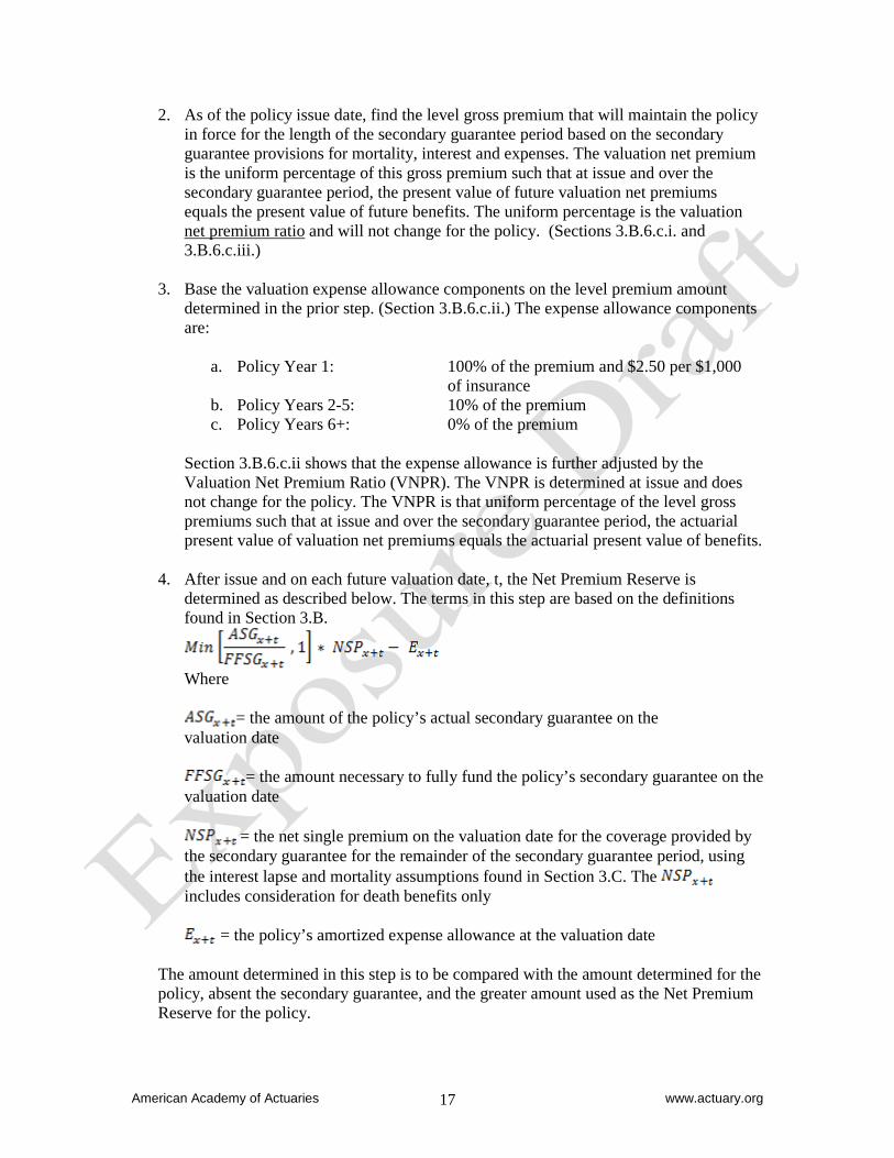
4. After issue and on each future valuation date, t, the Net Premium Reserve is
determined as described below. The terms in this step are based on the definitions found in Section 3.B.
Where
= the amount of the policy’s actual secondary guarantee on the
valuation date
= the amount necessary to fully fund the policy’s secondary guarantee on the valuation date
= the net single premium on the valuation date for the coverage provided by the secondary guarantee for the remainder of the secondary guarantee period, using the interest lapse and mortality assumptions found in Section 3.C. The includes consideration for death benefits only
= the policy’s amortized expense allowance at the valuation date
The amount determined in this step is to be compared with the amount determined for the policy, absent the secondary guarantee, and the greater amount used as the Net Premium Reserve for the policy.
American Academy of Actuaries www.actuary.org 18
Q4.5: How is the Net Premium Reserve calculated for policies with non-level death benefits or death benefits where the level of benefits is not guaranteed? A: Similar to the pre-principle-based reserve (pre-PBR) Standard Valuation Law, the NPR section of VM-20 was drafted in the context of a level premium level benefit annual premium contract. Adjustments to handle non-level benefits would generally follow the similar adjustments made today pre-PBR. The only item in the NPR calculation that specifically relates to benefits is the first year expense allowance of $2.50 per $1,000. No explicit instructions are included in VM-20 about whether a non-level death benefit would affect the first year value to which the $2.50 is applied, and therefore some actuaries would use the benefits payable in the first year. Q4.6: How is the Net Premium Reserve calculation affected if structural changes are made to the policy (i.e., changes separate from the automatic workings of the policy and initiated by the policyholder)? A: In the NPR calculation, some actuaries would follow the principles and practices that would apply under pre-PBR CRVM if there were structural changes to the policy. Q4.7: How are non-annual modes reflected in the Net Premium Reserve calculation? A: The Net Premium Reserve requirements were written to provide a standard for terminal reserves under an assumption of an annual mode premium similar to the pre-PBR formulaic requirements. Standard actuarial adjustments such as inclusion of a deferred premium asset or unearned premium reserve can be made to accommodate actual premium modes that are not annual. For flexible premium products, some actuaries would not calculate a deferred premium asset or unearned premium liability consistent with current actuarial practice pre-PBR. Q4.8: How are policy fees considered? A: For universal life products, the Net Premium Reserve approach uses a “solved-for” premium and, as a result, any policy fees required by the product would not directly enter into the calculation. For fixed premium term insurance products, the Net Premium Reserve approach requires the use of the maximum guarantee gross premium for the policy year as the gross premium used in setting the valuation net premium. Section 3 does not specifically discuss how policy fees enter into this calculation; however, some actuaries would include the policy fee for the policy in determining the uniform percentage of Section 3.B.7.a. Other actuaries would not include the policy fee, allowing the difference to be reflected in the uniform percentage factor. Q4.9: Do return of premium (ROP) products introduce any special considerations for the Net Premium Reserve? A: Section 3.B.7 requires the actuarial present value of future benefits to include death benefits, endowment benefits including endowments intermediate to the term of coverage, and cash surrender benefits. Some actuaries would conclude that “endowments” includes ROP benefits. All these benefits are determined before consideration for reinsurance and before consideration for policy loans in force. In the situation of a return of premium benefit
American Academy of Actuaries www.actuary.org 19
feature, all interim return amounts must be included in the Net Premium Reserve calculation. In this situation, Section 3.C.3.a. specifies a 0% lapse rate for non-fund based policies that provide non-forfeiture values. Q4.10: Is the Net Premium Reserve calculation similar to Universal Life Model Regulation Reserves (ULMR)? A: In terms of Section 3.B.5 (Net Premium Reserve for universal life without considering any secondary guarantee provisions) there are some similarities. However, while there are concepts that are similar, there are some differences. Both methods employ premium-solves at issue and at valuation date. However, the ULMR is solving for a maturity premium while the VM-20 method is solving for a premium that keeps the policy in force and not necessarily matures the policy. The “r” ratio is similar in that it is a ratio of actual policy account value to a solved-for account value, but in the context of ULMR, the solved-for account value considers maturity of the policy while in the context of VM-20, the solved-for account value considers only maintaining the policy in force. Q4.11: For fixed premium policies, if an interpolated terminal plus an unearned premium liability CRVM reserve is calculated instead of a mean reserve, would the actuary still need to calculate the Deferred Premium Asset? A: Terminal Net Premium Reserves are computed as of the end of a policy year and not the reporting date, so the terminal reserve as of policy anniversaries immediately prior and subsequent to the reporting date are adjusted to reflect that portion of the net premium that is unearned at the reporting date. This is generally accomplished using either the mean reserve method or the mid-terminal method. Other appropriate methods, including an exact reserve valuation, are also commonly used (see SSAP 51). Whatever valuation reserve method is used, the actuary may wish to confirm that all three components (Deterministic Reserve, Stochastic Reserve, Net Premium Reserve as adjusted for the reporting date) are internally consistent with respect to the assumption of premiums in the reserve. Consistency may be achieved by using the mean reserve method, the mid-terminal method or the exact reserve method with appropriate adjustments to the terminal Net Premium Reserve amount as summarized below. 1) Mean Reserve Method: Net Premium Reserve (using annual premium assumption) less
deferred premium asset; 2) Mid-Terminal Reserve Method: Net Premium Reserve (using annual premium
assumption) plus unearned premium reserve; 3) Exact Reserve Method: Net Premium Reserve (using actual premium mode for the
policy) with no adjustment needed. Q4.12: For flexible premium policies, would the actuary still need to calculate the Deferred Premium Asset? A: For fund based products with flexible premiums, some actuaries would not calculate a deferred premium asset or unearned premium reserve because the methodology results in a reserve that is consistent with the valuation date. Q4.13: Is the deferred premium asset on a gross or valuation net premium basis?
American Academy of Actuaries www.actuary.org 20
A: With respect to adjusting entries such as the deferred premium asset, the Net Premium Reserve methodology is intended to behave similar to the pre-PBR formulaic SVL methodologies. Some actuaries, therefore, would determine the DPA on a net basis and make any other adjustments consistent with pre-PBR adjustments. Q4.14: How would the actuary calculate the deferred premium asset for fixed premium policies in the first year? A: For term insurance based policies, the adjusted gross premium in the first year is zero, so the valuation net premium and the deferred premium asset in the first year would also be zero. For fixed premium universal life policies, the valuation net premium is a level percentage of the solved for gross premium so some policies may have a non-zero deferred premium asset. Q4.15: Are there any requirements with respect to the timing of benefits (i.e., curtate vs. continuous) in the Net Premium Reserve? A: The requirements are written in terms of an annual premium and some actuaries would interpret this as beginning of year timing. With respect to the benefits (death benefits, surrender benefits, etc.). Section 3 of VM-20 does not explicitly state requirements for the timing of such benefits. However, some actuaries would assume immediate payment of claims in the VM-20 reserve calculation as that is a current requirement of AG 32. Q4.16: How does the actuary apply the floors that are defined in Section 3.D? A: For a term insurance policy, some actuaries would compare the terminal Net Premium Reserve amounts to terminal cash value amounts and take the larger of the two. Then they would use these values to interpolate between policy anniversaries, and compare the result to the modal cost of insurance as described in Sections 3.D.1 and 2. Other actuaries may calculate the interpolated Net Premium Reserve amount prior to comparing to the consistently interpolated cash value amount and modal cost of insurance. There could be other methods that will develop as practice matures. Q4.17: Are lapse rates allowed in the NPR calculation? A: Section 3.C.3 specifies the lapse rates required to be used in the NPR calculation that varies by product type and by the number of guarantee years. Section 3.C.3.a specifies that lapses are allowed for universal life policies or riders which provide non-forfeiture values, universal life policies not containing a secondary guarantee, and universal life policies for which the longest secondary guarantee period is five (5) years or less. Q4.18: Are there specific lapse assumption required in the NPR calculation for level premium term products? A: Section 3.C.3.b. of VM-20 specifies the required lapse assumptions that must be used in the calculation. The rates vary based on the level premium period. If the level premium
American Academy of Actuaries www.actuary.org 21
period is less than 5 years, a 10% lapse rate is required to be used during the level premium period and for all other premium paying periods. If the level premium paying period is 5 or more years, then a 6% lapse rate is used during the level premium period. After an initial level premium period, the first renewal period lapse rate (also known as the shock lapse rate) varies by the level premium paying period, the length of the renewal premium guarantee and the percent increase in the gross premium per year (as specified in the table in Section 3.C.3.b.iv). After the first renewal period, the required lapse rate is 6%. Q4.19: Are there specific lapse assumptions required in the NPR calculation for Universal Life policies with secondary guarantees? A: If the secondary guarantee period is less than 5 years, then no lapse rates are allowed per Section 3.C.3.a of VM-20. Section 3.C.3.c specifies the formula for determining the lapse rates at each duration for policies with secondary guarantees greater than five years. Q4.20: Should assumed lapses occur annually, monthly, or on premium due dates? A: VM-20 does not provide any requirement as to the timing of assumed lapses or surrender benefits. Some actuaries will assume lapses occur on a basis consistent with how their cash flow testing is performed. It is common for a monthly assumption as to lapses to be made in future projections for those projection systems that process monthly cash flows. Some actuaries will assume shock lapses occur in the months after the initial level premium period expires based on historical experience. Other actuaries may assume average lapse rates during the year and process lapses on an annual basis. Q4.21: If the actuary expects policies to be limited pay, but they contractually allow for future premiums, what premium period should be used for the reserve calculation? A: For universal life policies, Sections 3.B.5 and 3.B.6 require the calculation of an annual premium for the period over which the premiums are permitted to be paid that would keep the policy in force over the entire period coverage is to be provided or under the provisions of the longest secondary guarantee. For term insurance policies, Section 3.B.4 requires the valuation net premium to be based on the maximum guaranteed gross premium. Two uniform percentages may be required for policies subject to the shock lapse provisions in Section 3.C.3.b.iv. Q4.22: How do the Net Premium Reserve interest rates compare to current SVL interest rates for term and universal life policies? A: Per Section 3.C.2.a, the valuation interest rate for term insurance policies with non-forfeiture benefits is the same as the current SVL. For term insurance policies without non-forfeiture benefits, the valuation interest rate is the same as the current SVL increased by 1.5%, but limited to 125% of the current SVL rate.
American Academy of Actuaries www.actuary.org 22
For universal life policies, the valuation interest rate differs for the Net Premium Reserve determined under Section 3.B.5 and Section 3.B.6. For calculation according to Section 3.B.5, the valuation interest rate is the same as the current SVL. For calculations according to Section 3.B.6, the valuation rate is the same as the current SVL increased by 1.5%, but limited to 125% of the current SVL rate.
American Academy of Actuaries www.actuary.org 23
5: VM-20 Calculation Overview – Part B. Deterministic Reserve Q5.1: How would actuaries approach the calculation of the Deterministic Reserve for each model segment as required by VM-20? A: VM-20 does not specify any specific steps to perform the Deterministic Reserve. Some actuaries may follow the approach described below. See Section 4 of VM-20 for more details.
a. Determine margins and prudent estimate assumptions for all risk factors as described in Section 9 of VM-20.
b. Determine the path of net asset earned rates as described in Section 7.H. c. Run the cash flow model to project liability cash flows. d. Calculate a gross premium reserve as the present value of future benefits and
expenses less the present value of future premiums and other revenue items using the path of net asset earned rates as the source of the discount rate.
Q5.2: What economic scenario assumptions are used to determine the Deterministic Reserve? A: Per Section 7.G.1, the Deterministic Reserve assumes the U.S. Treasury interest rate curves for Scenario 12 from the set of prescribed scenarios used in the stochastic exclusion ratio test (defined in Section 6.B of VM-20). The total investment return paths for general account equity assets and separate account fund performance also use those investment returns for corresponding investment categories contained in Scenario 12 from the set of prescribed scenarios used in the stochastic exclusion ratio test defined in Section 6.B. Q5.3: How does the actuary calculate the path of net asset earned rates? A: Section 7.H.4 states that the company must use the path of net asset earned rates as the discount rates for each model segment in the Deterministic Reserve calculations in Section 4. Therefore, as described in Section 7.H.1 and 7.H.2, for each model segment:
Determine a path of projected portfolio net asset earned rates for each projection interval used in the model (monthly, quarterly, annual, etc.). The net asset earned rate for each projection interval is calculated in a manner that is consistent with the timing of cash flows and length of the projection interval of the related cash flow model. The net asset earned rate for each projection interval will equal: Net Investment Earnings / Invested Assets The Net investment earnings term above includes:
Investment income (including any amortization of premium or accrual of discount) less appropriate default costs and investment expenses;
Capital gains and losses (excluding capital gains and losses transferred to the pretax interest maintenance reserve (PIMR));
Income from derivative asset programs; and Amortization of the PIMR.
American Academy of Actuaries www.actuary.org 24
Invested Assets are:
Determined in a manner that is consistent with the timing of cash flows within the cash flow model
Adjusted to reflect the negative of the outstanding PIMR Include the annual statement value of derivative instruments or a reasonable
approximation thereof.
Thus, the Net Asset Earned Rates will depend on: Projected Net Investment Earnings from the portfolio of starting assets Projected Net Investment Earnings from reinvestment assets The pattern of projected net liability cash flows (premiums less benefits and
expenses) Pattern of projected asset cash flows from starting assets and reinvestment
assets. However, per Section 7.H.2.a., separate account income and assets and interest (investment) income on policy loans and the policy loan asset are not included in the net asset earned rate calculation. VM-20 permits the use of simplified approaches to determine appropriate net asset earned rates if the approach used is consistent with the requirements of Section 2.G.
Q5.4: How will actuaries model assets in the deterministic and stochastic calculations? A: See Section 11 of this Practice Note for questions and answers about modeling of assets and the starting asset amount. Q5.5: How are separate account cash flows and balances reflected in the present value of future benefits calculations? A: Section 4.A.3.c states that the policy account value invested in the separate account at the valuation date is included as part of the actuarial present value of benefits. Section 4.A.4.b further states that future net cash flows between the general account and separate account for variable products are included in the actuarial present value of premiums and related amounts. Some actuaries would interpret these cash flows to include deposit of policyholder premiums to the separate account, transfers between fixed and variable investment options, transfers of separate account values to pay death or withdrawal benefits, and amounts charged to separate account values for cost of insurance, expense or other similar amounts. Q5.6: How is reinsurance incorporated into the Deterministic Reserve? A: Section 4.A.4.d states that future net reinsurance discrete cash flows are to be included as part of the present value of future premium and related amounts. Section 4.A.4.e states that future net reinsurance aggregate cash flows are also to be included in the present value of future premium and related amounts. For requirements regarding reinsurance cash flows, refer to VM-20 Section 8.
American Academy of Actuaries www.actuary.org 25
6: VM-20 Calculation Overview – Part C. Stochastic Reserve Q6.1: How is the Stochastic Reserve determined as required by VM-20? A: Section 5 of VM-20 contains the requirements for determining the Stochastic Reserve (all references below are to VM-20).
a. Determine margins and Prudent Estimate Assumptions for all Risk Factors as described in Section 9.
b. Generate the stochastic economic scenarios as described in Section 7.G.2. c. Determine the number of stochastic economic scenarios to use in the calculation as
described in section 7.G.2.c, d and e. d. Determine the number of subgroups for aggregation purposes for the Stochastic
Reserve calculation as described in Section 7.B.3. e. For each subgroup calculate the Stochastic Reserve as follows:
1. Project cash flows for each Model Segment under each economic scenario as described in Section 5.
2. Determine the Scenario Reserve for each scenario as described in Section 5.B.3.
3. Calculate the Stochastic Reserve by ranking the Scenario Reserves from lowest to highest and taking the average of the highest 30% (CTE 70) of these Scenario Reserves.
f. Add together the Stochastic Reserve for all aggregation subgroups. g. If necessary, add amounts to the Stochastic Reserve to capture any material risk
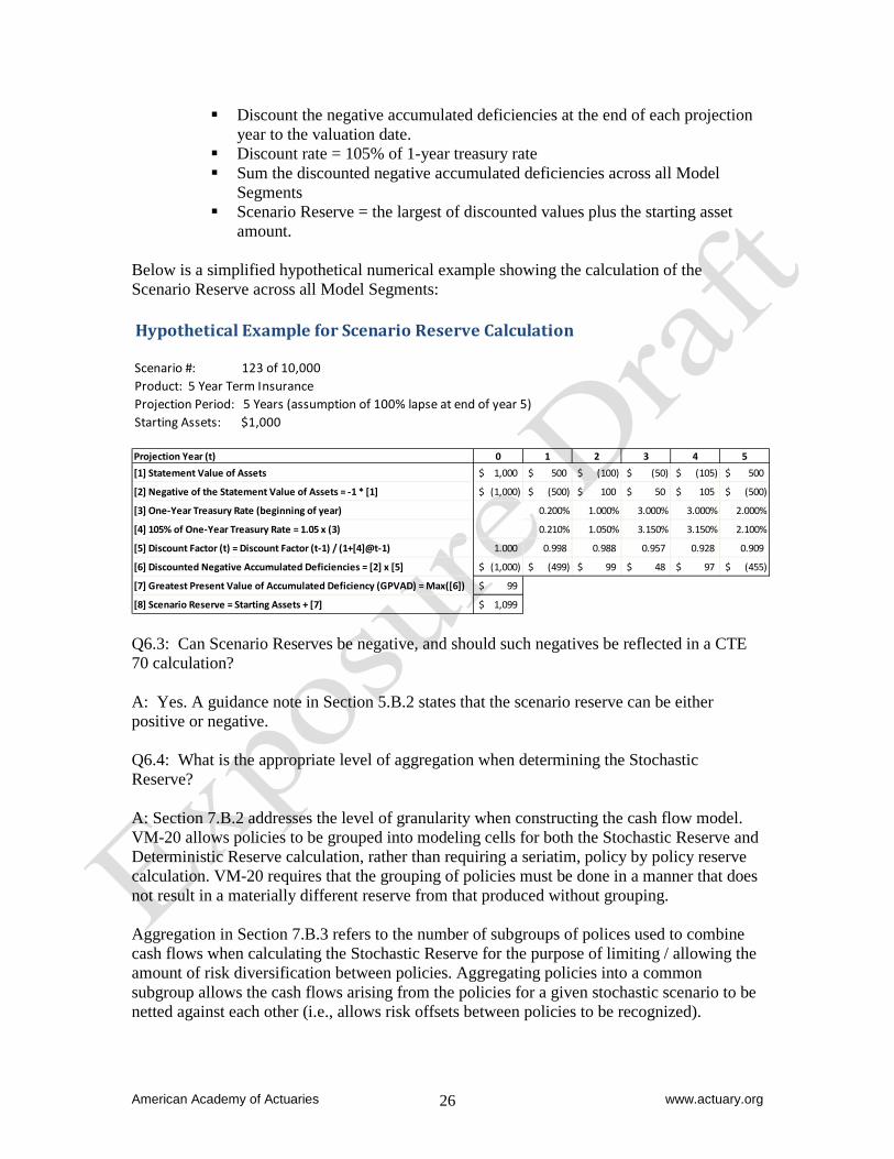
included in the scope of VM-20 but not already reflected in the Stochastic Reserve. Q6.2: How is the Scenario Reserve calculated? A: Section 5.B describes how the Scenario Reserve is calculated. The Scenario Reserve is calculated at the aggregation subgroup level not the model segment level. A Model Segment is defined in Section 1.C.7 of VM-20 and discussed in Section 7.A.1.b. It is a group of policies with a similar investment strategy. If a company is managing the risks of two or more different product types as part of an integrated risk management process, then the products may be combined into the same subgroup (an aggregation subgroup). The guidance note in Section 7.B.3 states that aggregating policies into a common subgroup allows the cash flows arising from the policies for a given stochastic scenario to be netted against each other. A scenario reserve is the negative of the present value of accumulated net cash flows at the beginning or end of the year when the accumulated deficiency is the most negative during the projection period. This method is often called the Greatest Present Value of Accumulated Deficiency (GPVAD). In this method, future sufficiencies past the minimum point are not taken into account in the calculation. The reserve for each scenario is determined as follows:
At the valuation date, and at the end of each projection year, calculate the negative of the projected statement value of assets (may be positive or negative) for all model segments. The negative of the projected statement value of assets is called the negative accumulated deficiency.
American Academy of Actuaries www.actuary.org 26
Discount the negative accumulated deficiencies at the end of each projection year to the valuation date.
Discount rate = 105% of 1-year treasury rate Sum the discounted negative accumulated deficiencies across all Model
Segments Scenario Reserve = the largest of discounted values plus the starting asset
amount. Below is a simplified hypothetical numerical example showing the calculation of the Scenario Reserve across all Model Segments: Hypothetical Example for Scenario Reserve Calculation
Scenario #: 123 of 10,000Product: 5 Year Term InsuranceProjection Period: 5 Years (assumption of 100% lapse at end of year 5)Starting Assets: $1,000
Projection Year (t) 0 1 2 3 4 5[1] Statement Value of Assets 1,000$ 500$ (100)$ (50)$ (105)$ 500$
[2] Negative of the Statement Value of Assets = -1 * [1] (1,000)$ (500)$ 100$ 50$ 105$ (500)$
[3] One-Year Treasury Rate (beginning of year) 0.200% 1.000% 3.000% 3.000% 2.000%
[4] 105% of One-Year Treasury Rate = 1.05 x (3) 0.210% 1.050% 3.150% 3.150% 2.100%
[5] Discount Factor (t) = Discount Factor (t-1) / (1+[4]@t-1) 1.000 0.998 0.988 0.957 0.928 0.909
[6] Discounted Negative Accumulated Deficiencies = [2] x [5] (1,000)$ (499)$ 99$ 48$ 97$ (455)$
[7] Greatest Present Value of Accumulated Deficiency (GPVAD) = Max([6]) 99$
[8] Scenario Reserve = Starting Assets + [7] 1,099$ Q6.3: Can Scenario Reserves be negative, and should such negatives be reflected in a CTE 70 calculation? A: Yes. A guidance note in Section 5.B.2 states that the scenario reserve can be either positive or negative. Q6.4: What is the appropriate level of aggregation when determining the Stochastic Reserve? A: Section 7.B.2 addresses the level of granularity when constructing the cash flow model. VM-20 allows policies to be grouped into modeling cells for both the Stochastic Reserve and Deterministic Reserve calculation, rather than requiring a seriatim, policy by policy reserve calculation. VM-20 requires that the grouping of policies must be done in a manner that does not result in a materially different reserve from that produced without grouping. Aggregation in Section 7.B.3 refers to the number of subgroups of polices used to combine cash flows when calculating the Stochastic Reserve for the purpose of limiting / allowing the amount of risk diversification between policies. Aggregating policies into a common subgroup allows the cash flows arising from the policies for a given stochastic scenario to be netted against each other (i.e., allows risk offsets between policies to be recognized).
American Academy of Actuaries www.actuary.org 27
Full aggregation means that the cash flows for all policies are combined together in one group. In contrast, an actuary may decide to group policies into one or more subgroups. VM-20 requires that the level of aggregation must be consistent with how the company manages risks across the different product types and must reflect the likelihood of any change in risk offsets that could arise from shifts between product types. For example, if a company is managing the risks of two or more different product types as part of an integrated risk management process, then the products may be combined into the same aggregation subgroup. Some actuaries believe that the level of aggregation is up to actuarial judgment, consistent with the risk appetite of the company. Other actuaries believe that risk diversification is a key principle of a principle-based approach, and therefore, full aggregation is appropriate. Therefore, these actuaries would aggregate all policies together (full aggregation), while other actuaries may look toward company practices for managing the business (e.g., what is used for cash flow testing purposes) as a basis for defining two or more aggregation subgroups. The rationale for an actuary’s decision to aggregate policies for risk diversification is to be documented as part of the Actuarial Report. Making a change of aggregation solely to obtain a more favorable outcome is not within the spirit of principle-based calculations and would not be a reasonable justification for making such a change. Q6.5: Would an actuary aggregate a term and universal life product in the VM-20 calculation? A: If the company’s practice is to manage the risk of term and universal life products together (e.g., same investment portfolio for both products, and/or some aspects of the determination of the expected mortality is the same), then some actuaries would perform the calculation of the VM-20 reserves for these products on an aggregated basis. Of course, there would be some requirement to allocate the Stochastic Reserve to each policy separately for financial reporting purposes. Other actuaries would perform the calculation of the VM-20 Stochastic Reserve separately but would use many of the same assumptions. The rationale here would be that the blocks may have similar calculations but essentially have enough differences that it is appropriate to project separately. Q6.6: Will term insurance products with different level premium periods be projected in an aggregated basis or separately in the Stochastic Reserve? A: Some actuaries may model all of the level term products in one model in aggregate because the products are managed together and are believed to have similar risks. Other actuaries may combine some level premium periods but model others separately (e.g., 30 year level premium period) because they believe that the product risks are different. Also some actuaries may model each different level premium period separately because the risk for each level premium period is managed separately or they believe separate models are more appropriate. Q6.7: Are the prudent estimate assumptions the same for the Stochastic Reserve as for the Deterministic Reserve? A: Per Section 9.A.5 prudent estimate assumptions for the stochastic and Deterministic Reserve must be consistent, with an exception for assumptions that are dependent (i.e.,
American Academy of Actuaries www.actuary.org 28
dynamically linked) on the economic scenario, such as lapse rates that move up or down with changes in interest rates. Q6.8: Does the calculation of the Stochastic Reserve include the use of a “working reserve” similar to the AG43? A: VM-20 does not mention “working reserves.” This is equivalent to a working reserve equal to zero. Q6.9: How are the discount rates determined?
A: Per Section 7.H.5, the discount rates for the Stochastic Reserve are set equal to the path of the beginning of year one-year treasury rates for the scenario, multiplied by 1.05. The guidance note in this section has additional information on why this discount rate was chosen and why it is different from the one used for the Deterministic Reserve. Q6.10: How does the actuary determine the amount (if any) to add to the Stochastic Reserve to capture any material risk not already reflected in the Stochastic Reserve per Section 5.E of VM-20? A: VM-20 is not specific on how this adjustment will be determined. Some actuaries may make an adjustment for material risks where it is known that their Stochastic Reserve models do not cover specific policy risks. For example, if there is a certain rider that would pay an additional benefit if some contingent event happened and that event is not being modeled, then the actuary may include an adjustment for the payment of this benefit.
American Academy of Actuaries www.actuary.org 29
7. Stochastic Exclusion Test Q7.1: What is the Stochastic Exclusion Test? A: As described in Section 6 of VM-20, the Stochastic Exclusion Test can be used to identify groups of policies that do not have material interest rate or asset return volatility risk, and therefore do not have significant variation in financial results dependent upon future economic conditions. Companies may elect to use this test to exclude groups of policies from the calculation of the Stochastic Reserve. Q7.2: What methods are available to pass the Stochastic Exclusion Test? A: The actuary may use any of three approaches to pass the Stochastic Exclusion Test. One approach, the Stochastic Exclusion Ratio Test, as described in Section 6.A.2, is to run 16 specified scenarios that are used in a ratio to demonstrate minimal variation by economic scenario in the present value of cash flows. Alternatively, as described in Section 6.A.3, the actuary can demonstrate that the Stochastic Reserve would not increase the minimum reserve required for the group of policies. The third approach that can be used only for policies that are not variable life or not universal life with secondary guarantees, is for a qualified actuary to certify and report that the policies are not subject to material interest rate risk or tail risk, or asset risk. Q7.3: What products might be good candidates for the Stochastic Exclusion Test? What products may not be excluded? What products are only allowed to pass the test under specific testing methods? A: Life insurance products where the main risks are not highly dependent on interest rate movements or equity performance, or where these types of risks can be shared or passed on to the policyholder are strong candidates for the Stochastic Exclusion Test. Some actuaries may use the Stochastic Exclusion Test for products such as term life insurance, which focus primarily on mortality risk, or for some variations of traditional permanent life insurance and accumulation-oriented universal life insurance where non-guaranteed elements help transfer the asset performance risk to the policyholder. Variable life or universal life insurance products that contain secondary guarantees may not use a certification method to pass the Stochastic Exclusion Test. These types of policies may only be excluded through the use of the Stochastic Exclusion Ratio Test or the Stochastic Exclusion Demonstration Test under Section 6.A.3. Q7.4: Can a group of policies with a clearly defined hedging program be excluded from calculating the Stochastic Reserve? A: No. Section 6.A.1.b states that a company may not exclude a group of policies for which there is one or more clearly defined hedging strategies from the Stochastic Reserve requirements. Q7.5: Is it necessary to perform the Stochastic Exclusion Test on all blocks of life insurance? A: No. Section 2.D.3 states if a company elects to calculate Stochastic Reserves for one or more groups of policies, the Stochastic Exclusion Test is optional for those groups of
American Academy of Actuaries www.actuary.org 30
policies. In other words, the test may be performed for all groups within the entire in force life insurance business, for selected blocks of business, or for none of the business. Q7.6: How does a company determine whether a group of policies passes the Stochastic Exclusion Ratio Test? A: The Stochastic Exclusion Ratio Test is one method to pass the Stochastic Exclusion Test thereby excluding a group of policies from calculation of Stochastic Reserves. The company calculates a ratio that evaluates the sensitivity of the reserve to changes in the economic scenario. The numerator of the ratio is equal to the difference between two items: the Adjusted Deterministic Reserve calculated under a baseline economic scenario, and the largest Adjusted Deterministic Reserve calculated under any of the 15 other economic scenarios. The method for creating the economic scenarios is found in Appendix 1 of VM-20 and can be produced using the prescribed Economic Scenario Generator. The Adjusted Deterministic Reserve is calculated similarly to the Deterministic Reserve in Section 4.A, but with adjustments specified in Section 6.A.2.b. The denominator of the Stochastic Exclusion Ratio Test is the present value of benefits for the group of policies, as determined in the baseline economic scenario, with an adjustment to reflect reinsurance by subtracting out ceded benefits. If the ratio of the numerator over the denominator is less than 4.5%, it implies that the reserve calculation is relatively insensitive to variation in economic scenarios, and the group of policies passes the Stochastic Exclusion Ratio Test. Q7.7: What are the differences between the Adjusted Deterministic Reserve in the numerator of the Stochastic Exclusion Ratio Test and the Deterministic Reserve? A: The adjusted Deterministic Reserve in the numerator of the test is calculated similarly to the Deterministic Reserve in Section 4.A. However, changes are made in order to adjust the reserve calculation as described in Section 6.A.2.b. In particular, anticipated experience assumptions used in the Adjusted Deterministic Reserve calculation include no margins, whereas the corresponding assumptions for the Deterministic Reserve would include margins. Similarly, net asset earned rates used across the variety of scenarios in calculating the Adjusted Deterministic Reserves are specific to each scenario in order to discount cash flows, whereas the discounting assumption in the Deterministic Reserve would be based on one specified scenario. As in the calculation of the Deterministic Reserve, the Adjusted Deterministic Reserve should still use dynamic adjustments for experience assumptions that depend on the economic scenario. Q7.8: Can the actuary include mortality improvement beyond the valuation date when performing the Stochastic Exclusion Ratio Test?
American Academy of Actuaries www.actuary.org 31
A: No, per Section 6.A.2.b.v, mortality improvement past the projection start date is not allowed in the anticipated experience assumptions used in the Stochastic Exclusion Ratio Test. Q7.9: What amounts should be included and excluded from the present value of benefits in the denominator of the Stochastic Exclusion Ratio Test? A: The present value of the benefits used in the denominator of the Stochastic Exclusion Ratio Test specifically should include benefits (net of benefits ceded through reinsurance) such as death benefits, surrenders, withdrawal benefits and policyholder dividends. Section 6.B.2.a.iii states that premium, ceded premium, expenses, reinsurance expense allowances, modified coinsurance reserve adjustments and reinsurance experience refund cash flows may not be included in the calculation of the benefit amount. Q7.10: How does the company create the 16 economic scenarios used for the Stochastic Exclusion Ratio Test? A: The methodology for creating the 16 economic scenarios is defined in Appendix 1 of VM-20. Q7.11: Are there other requirements the actuary should understand when determining the minimum reserve requirement for a group of policies passing the Stochastic Exclusion Test? A: If a group of policies passes the Stochastic Reserve Exclusion Test, then Stochastic Reserve calculations are not required in determining the minimum reserve. If the Stochastic Exclusion Test is relied upon to avoid calculating the Stochastic Reserve, then, according to Section 4.A.5, future transactions associated with non-hedging derivative programs may not be included in calculating the Deterministic Reserve. If the Stochastic Exclusion Ratio Test is used to pass the Stochastic Exclusion Test, the demonstration must be done annually and within 12 months before the valuation date. Some actuaries may still calculate the Stochastic Reserve and use it in the determination of the minimum reserve even if the block of business passed the Stochastic Exclusion Test. Q7.12: What happens if a group of policies fails the Stochastic Exclusion Test? A: If a group of policies fails the test, both the Stochastic Reserve and Deterministic Reserve must be calculated for that group of policies. Section 2.A.3 remains the definition of the minimum reserve in this situation. Q7.13: How does a company demonstrate that a group of policies passes the Stochastic Exclusion Test because it is not subject to material risks? What methods are acceptable? What information is needed? What demonstrations and reports need to be prepared? A: Section 6.A.3 outlines several methods that may be used to demonstrate that the group of policies is not subject to material risk. The company may opt to show that the greater of the Deterministic Reserve and the Net Premium Reserve is greater than the Stochastic Reserve.
American Academy of Actuaries www.actuary.org 32
Alternatively, the company may show that the greater of the Deterministic Reserve and the Net Premium Reserve is greater than a scenario reserve in each of a sufficient number of adverse deterministic scenarios. The company may also show that the greater of the Deterministic Reserve and Net Premium Reserve is greater than the Stochastic Reserve calculated on a standalone basis, but using a smaller representative subset of the policies in the stochastic calculation, rather than the entire group of policies. The company may also show that the main risk characteristics that would drive the Stochastic Reserve to exceed the larger of the Deterministic Reserve and the Net Premium Reserve have been substantially mitigated through various company actions. These actions may include hedging, risk reducing investment strategies, reinsurance, or transferring of the risk to the policyholder through contractual provisions. The company may also use another method that is acceptable to the commissioner. If any of these methods are used, the company must provide a demonstration in the PBR Actuarial Report. The demonstration must provide reasonable assurance that if the Stochastic Reserve was calculated, the minimum reserve would not increase. The report must be prepared in the first year that the demonstration is performed, and at least once every three years thereafter. Q7.14: How would the qualified actuary certify that a group of policies may be excluded from the Stochastic Reserve calculation? A: Per the Guidance Note in Section 6.A.1.a.iii, the qualified actuary should develop documentation to support the actuarial certification that presents the analysis clearly and in detail sufficient for another actuary to understand the analysis and reasons for the actuary’s conclusion that the group of policies is not subject to material interest rate risk or asset return volatility risk. Examples of methods a qualified actuary could use to support the actuarial certification include, but are not limited to: 1. A demonstration that reserves for the group of policies calculated according to Sections 5–9 of VM-05, VM-A and VM-C are at least as great as the assets required to support the group of policies using the company’s cash flow testing model under each of the 16 scenarios identified in Section 6 or alternatively each of the New York 7 scenarios. 2. A demonstration that the group of policies passed the stochastic exclusion ratio test within 36 months prior to the valuation date and the company has not had a material change in its interest rate risk. 3. A qualitative risk assessment of the group of policies that concludes that the group of policies does not have material interest rate risk or asset return volatility. Such assessment would include an analysis of product guarantees, the company’s non-guaranteed element policy, assets backing the group of policies and the company’s investment strategy. Q7.15: What analysis would be done on a regular basis for groups of policies that satisfy the Stochastic Exclusion Test? A: Some actuaries would review the characteristics of each group of policies on a regular basis to make sure that the group of policies still passes the test particularly if the block only
American Academy of Actuaries www.actuary.org 33
passed the test by a small margin. Other actuaries may identify certain economic parameters or other characteristics of the block of policies that drives variability to economic conditions and would monitor those items to see if the calculations need to be recomputed. An example of this may be a block of universal life policies without secondary guarantees, with cash values that are a very low percentage of the death benefit. It may be that this block is not currently sensitive to economic conditions but if the cash values increase, the sensitivity of that block could increase to the point where it no longer passes the test. Other actuaries may only perform the test when it is required under VM-20 if they believe the block has not changed enough to make re-testing worthwhile. Q7.16: If a group of policies becomes subject to material risks after having previously been certified, what transition does the company need to make in light of the Stochastic Exclusion Test? A: In this situation, the company would need to reevaluate whether the group of policies requires a calculation of the Stochastic Reserve. It may be that the group of policies still satisfies one of the other exclusion tests or if not, the exclusion needs to be discontinued. The company would then be required to calculate Stochastic Reserves in the determination of the minimum reserve according to Section 6.A.3.a.ii. Q7.17: Does the Stochastic Exclusion Test need to be performed with year-end valuation data? A: According to Section 6.A.1.a.i, groups of policies pass the stochastic exclusion test if annually and within 12 months before the valuation date the company demonstrates that the groups of policies pass the stochastic exclusion ratio test defined in Section 6.A.2. Therefore, year-end data does not need to be used.
American Academy of Actuaries www.actuary.org 34
8: Deterministic Reserve Exclusion Test Q8.1: What is the Deterministic Reserve Exclusion Test? A: The Deterministic Reserve Exclusion Test (also referred to as the Deterministic Exclusion Test) is a test that a company may elect to perform in order to simplify its valuation process. If a group of policies passes both the Stochastic Exclusion Test and the Deterministic Reserve Exclusion Test, then Section 2.A.1 notes that the minimum reserve would be the aggregate Net Premium Reserves for those policies. In other words, the Deterministic Reserve does not need to be calculated for those policies. However, if the group of policies passes the Deterministic Reserve Exclusion Test but not the Stochastic Reserve Test, then both the Deterministic Reserve and the Stochastic Reserve must be calculated. Q8.2: How would a group of policies pass the Deterministic Reserve Exclusion Test? A: As described in VM-20, Section 6.B, a group of policies passes, the Deterministic Reserve Exclusion Test when the company demonstrates that the sum of valuation net premiums for all future years is less than the sum of the corresponding guaranteed gross premiums. A company may elect to perform this test for a group of policies, only if the group has passed the Stochastic Reserve Exclusion Test, to determine if they are required to calculate the Deterministic Reserve for that group of policies. Q8.3: Is it necessary to perform the Deterministic Reserve Exclusion Test on all blocks of life insurance? A: No. Section 2.A and 2.D note that the Deterministic Reserve Exclusion Test is optional. The test may be applied to all groups within the entire in force life insurance business, to selected groups of policies, or not be applied at all. Q8.4: Are there any types of products that cannot be excluded from calculating the Deterministic Reserve through the Deterministic Reserve Exclusion Test? A: Section 6.B.1 specifically notes two types of policy groups that are automatically deemed to not pass the Deterministic Reserve Exclusion Test. The first are universal life policies with a secondary guarantee. The second are groups of policies which are not excluded from the Stochastic Reserve calculation. Deterministic Reserves must be calculated for these policies. Q8.5: What limitations exist for grouping policies when using the Deterministic Reserve Exclusion Test? A: Section 6.B.3 states that different contract types may not be grouped together for a combined test if the contract types present significantly different risk profiles. Many actuaries would use the same grouping for the Stochastic Exclusion Test and the Deterministic Reserve Exclusion Test due to the similar requirements of Section 6.A.2.b.iv and 6.B.3. For example, a block of policies with high guaranteed gross premiums relative to their valuation net
American Academy of Actuaries www.actuary.org 35
premiums may have less mortality risk than other blocks within the company. Many actuaries would not combine this block with other contract types that have high mortality risk in order for the combined group collectively to pass the Deterministic Reserve Exclusion Test. It would be prudent for actuaries who are expecting to calculate both the Stochastic Exclusion Test and the Deterministic Reserve Exclusion Test, to consider the grouping requirements for both tests when determining the appropriate grouping for modeling the policies. Q8.6: What valuation net premiums are used in the Deterministic Reserve Exclusion Test? A: The valuation net premiums used in the Deterministic Reserve Exclusion Test are defined in VM-20 Section 6.B.5 as follows: For policies where the Net Premium Reserve is the minimum reserve according to the minimum reserve requirements of Section 2.A of the Standard Valuation Law that applied to policies issued prior to the Valuation Manual becoming effective (see VM-A and VM-C), then the valuation net premiums are determined according to those minimum reserve requirements. For term life insurance or for universal life insurance with a secondary guarantee, the valuation net premium is derived from applying Section 3 of VM-20 with lapse rates set to zero for all durations per Section 6.B.5.b. For any group of policies, if anticipated mortality is expected to be higher than the valuation mortality for the group of policies, then anticipated mortality must be used in the determination of the valuation net premium. Q8.7: What gross premiums are used in the Deterministic Reserve Exclusion Test? A: Per Section 6.B.5.e, guaranteed gross premiums used in the Deterministic Reserve Exclusion Test will generally be the guaranteed gross premiums specified in the contract. For some universal life policies, there may not be a schedule of guaranteed gross premiums. If no guaranteed gross premiums are specified, VM-20 defines the gross premium to use as the level annual gross premium at issue that will keep the life insurance policy in force for the entire coverage period based on the policy guarantees. Q8.8: Is the comparison of valuation net premiums and guaranteed gross premiums done before (direct) or after reinsurance? A: Per Section 6.B.2, the test is performed on either a direct or assumed basis. This means it is performed before reinsurance ceded and including all assumed business. Q8.9: What products might be good candidates for the Deterministic Reserve Exclusion Test? A: Traditional products that have guaranteed gross premium levels in excess of valuation net premiums are good candidates for the Deterministic Reserve Exclusion Test. These product types generally have gross premiums that provide sufficient revenues to cover adverse
American Academy of Actuaries www.actuary.org 36
development of mortality, expense or investment income experience. However, the Deterministic Reserve Exclusion Test is not mandatory and some actuaries may calculate the Deterministic Reserve even for policies that likely would pass the test. Q8.10: What are the implications of a block of business passing the Deterministic Reserve Exclusion Test? A: If a block of business passes the Deterministic Reserve Exclusion Test, then Deterministic Reserve calculations are not required in determining the minimum reserve. Some actuaries may still calculate the Deterministic Reserve, however, and use it in the determination of the minimum reserve. Q8.11: How frequently is the Deterministic Reserve Exclusion Test performed? Section 6.B.4 states that for a group of policies that is no longer adding new issues and the test has been passed for three consecutive years, the test is assumed to be passed each year as long as the test is computed once each five years going forward. Some actuaries see this requirement as implying that the test is required to be passed annually unless the group of policies meets the requirements of Section 6.B.4. There is no specific requirement in VM-20 on how often the test must be performed. Some actuaries would perform the test annually as of the valuation date. Other actuaries would perform the Deterministic Reserve Exclusion Test in conjunction with the Stochastic Reserve Exclusion Test if the group of policies is eligible for passing the Deterministic Reserve Exclusion Test. Q8.12: What changes may occur that could cause a group of policies where no new business is being issued in that group to fail the Deterministic Reserve Exclusion Test after passing for several consecutive years? A: Significant changes in the risk profile of a group of policies could cause a group of policies that had been passing to start failing the test. For example, if poor experience emerges in the group over time that has sufficient credibility, then the actuary may change the future anticipated mortality assumption such that may begin to approach or exceed the valuation mortality. In this case, the new, higher anticipated mortality will be used to determine valuation net premiums, and the resulting net premiums may be higher than the guaranteed gross premiums for the group.
American Academy of Actuaries www.actuary.org 37
9. Difference from Cash Flow Testing – Scenario Reserve Calculation Q9.1: May the actuary use an asset adequacy testing cash flow model to calculate the scenario reserve in the stochastic reserve calculation for VM-20? A: Some actuaries will make use of their cash flow testing (CFT) models in calculating the scenario reserve. However, the actuary may need to adjust the CFT model to reflect the different purposes of the calculations. Some of the potential differences between CFT and VM-20 are listed below. Note that this list is not intended to be a complete listing of all differences.
• CFT models may have some approximations or model simplifications that are not appropriate for VM-20.
• CFT may be based on assumptions that are not prudent estimate assumptions; VM-20 uses prudent estimate assumptions.
• Some assumptions in VM-20 are prescribed and must be used in the calculation. CFT has no prescribed assumptions.
• There may be some difference in projection periods / timestep / model segments. • Some business where the scenario reserve needs to be determined may not be cash
flow tested. • The starting assets used in the model and reinvestment assumptions may be different. • Cash flow testing models may include issue years that are not within the scope of
VM-20. • Treatment of IMR and AVR may be different.
Q9.2: May the actuary use the same assumptions for VM-20 as those used for cash-flow testing? A: VM-20 Section 9.A.1 requires that prudent estimate assumptions must be used. Section C, Definition 17 defines prudent estimate assumptions as “a risk factor assumption developed by applying a margin to the anticipated experience assumptions for that factor.” Some modifications to cash flow testing assumptions may be required if the cash flow testing assumptions are not prudent estimate assumptions. Also, there are some assumptions that are fully or partially prescribed for the Stochastic Reserve calculation. Examples include lapse rates for certain Universal Life policies per Section 9.D.5 and asset reinvestment and default assumptions as described in Section 9.F. Q9.3: In calculating the Stochastic Reserve, may the actuary use the same interest rate and equity scenarios as used for the CFT projections? A: Section 7.G.2.a states that a prescribed economic scenario generator with prescribed parameters is required to be used to generate the interest rate and equity scenarios used in the determination of the Stochastic Reserve. Scenario reduction techniques are allowed but only if they do not materially reduce the reserve. CFT analysis does not require the same generator and parameters. However, some actuaries may use the prescribed VM-20 scenarios for CFT analysis if the actuary believes the scenarios are appropriate.
American Academy of Actuaries www.actuary.org 38
Q9.4: Can the CFT projection period be used without modification for VM-20 calculations? A: Section 7.A.1.d of VM-20 states that “The Company shall use a cash flow model that projects for a period that extends far enough in the future so that no obligations remain.” There is also a Guidance Note in this section that states “For example, it may be reasonable to assume 100% deaths or 100% surrenders after some appropriate period of time. Actuaries wishing to use the same projection period in the VM-20 calculation as is used for CFT will have to make sure these conditions are satisfied. Q9.5: Would the actuary generally use the same starting assets in both the VM-20 and CFT calculations? A: Section 7.D requires the assignment of a set of starting assets satisfying certain criteria to each model segment. Some actuaries will assign the same assets for both calculations but it is not a requirement. Since VM-20 applies to new issues only, some actuaries may select a limited sub set of assets that were purchased during the time period when the sales occurred and that meet the criteria. Other actuaries may use a pro-rata portion of the CFT assets for VM-20 if these assets meet the criteria. Q9.6: Would the actuary generally use the same model aggregation in VM-20 as that is used in the CFT calculations? A: Section 7.B.3 states that “In determining the Stochastic Reserve, the company shall determine the number and composition of subgroups for aggregation purposes in a manner that is consistent with how the company manages risks across the different product types, and that reflects the likelihood of any change in risk offsets that could arise from shifts between product types. If a company is managing the risks of two or more different product types as part of an integrated risk management process, then the products may be combined into the same subgroup.” Actuaries wishing to use the same aggregation in calculating the scenario reserve as they use in the CFT must verify that they are in compliance with this section of VM-20. Q9.7: How are IMR and AVR treated in Stochastic and Deterministic Reserve calculations? A: Section 7.D.2.d. says to allocate the negative of any pre-tax IMR to each model segment at the projection start date. Section 7.H.2.c.iii. says that net investment earnings include amortization of the PIMR. VM-20 Section 7.I. states that future capital gains and losses arising from changes in interest rates should be added to the PIMR and amortized assuming the capital gains tax is zero. Q9.8: How are federal income taxes treated in VM-20 versus CFT? A: VM-20 requires that federal income taxes be excluded from cash flows. Typically, federal income taxes would be reflected in CFT.
American Academy of Actuaries www.actuary.org 39
Q9.9: Are taxes other than federal income taxes ignored for the purpose of calculating reserves under VM-20? For example, should the actuary ignore premium taxes? A: Section 7.B.1.e states that taxes (excluding federal income taxes and expenses paid to provide fraternal benefits in lieu of federal income taxes) should be included in the cash flows. Section 9.E contains more information on taxes and expenses that should be included including that foreign income taxes are excluded (Section 9.E.1.g).
American Academy of Actuaries www.actuary.org 40
10. Considerations When Performing Work on Other Than the Valuation Date Q10.1: What valuation date is required for the Stochastic and Deterministic Reserve? A: Per Section 2.E of VM-20, the calculation of the Stochastic and Deterministic Reserve can be performed as of a date up to three months prior to the Valuation Date as long as an appropriate method is used to adjust the reserves to the Valuation Date. Section 3.3.5 of the discussion draft of a proposed ASOP on Principle-Based Reserves suggests the use of a Deterministic Update, but warns of conditions that could require adjustment such as condition changes that affect guarantees (this is a discussion draft only and not an exposure draft of any ASOP and its contents have not been reviewed or approved by the ASB and is therefore subject to changes). Although the calculation may use prior data, some actuaries would take into account relevant experience up to the Valuation Date in their determination of Anticipated Experience and Prudent Estimate Assumptions used in the calculations. Q10.2: Does the Net Premium Reserve have to be calculated using data as of the valuation date? A: The Net Premium Reserve is a seriatim reserve that is calculated for each policy inforce on the valuation date. It is expected that actuaries would perform the Net Premium Reserve calculation as of the valuation date using current in force data, if possible. Q10.3: How might an actuary “use an appropriate method to adjust” the Deterministic and Stochastic reserve to the valuation date when it is calculated as of an earlier date? A: VM-20 does not prescribe a method for this. Some actuaries may use a model office as of the earlier date and make several adjustments to take into account changes to the valuation date. The adjustments could include taking into account lapses and new policies issued since the model date but prior to the valuation date through a pro-rata adjustment to the relevant policy information (e.g., face amount, account value) so the overall characteristics for the group of policies approximate those characteristics on the valuation date. Additionally, the actuary could review all prudent estimate assumptions in the model and make any adjustments necessary for information / experience from the model date to the valuation date. Adjustments to the assets may or may not be made depending on how materially the asset portfolio has changed. Many actuaries would use the economic scenarios as of the valuation date in particular if the economic conditions have changed materially. Some actuaries may apply a high level adjustment to the overall reserve amount or to each of several portions of the reserve. The adjustment may be based on analysis of past trends in the reserve, including “roll-forward” analysis of the change in the reserve balance. Such analysis would typically isolate the main drivers of the reserve change and would enable the actuary to estimate short term changes in the reserve after the calculation date based on correlation with those drivers. This could include using some characteristic of the group of policies in the calculation (e.g., face amount for a group of term insurance policies) and a ratio method to modify the Scenario Reserve for the stochastic calculation or the Deterministic Reserve for the group of policies actually in force on the valuation date. Other actuaries may calculate the Stochastic and Deterministic Reserve on a small, representative sample of policies from the
American Academy of Actuaries www.actuary.org 41
group of policies on the valuation date and compare this amount to the Stochastic and Deterministic Reserve for those policies as of the prior calculated date. This information could be used in a number of ways to modify the calculations made using the prior date to the valuation date. Of course, the actuary would need to be prudent in determining the number of representative samples that are appropriate and which policies to use in this calculation. It would be prudent for the actuary to confirm that the approach used is appropriate for the group of policies being valued. If the policy characteristics or economic environment have changed materially, a valuation date prior to the reporting date may not be appropriate. Q10.4: Should changes in economic conditions from the Projection Start Date also be incorporated in the adjustment of the reserves? A: Many actuaries performing the calculations would modify the reserve calculations to take into account the economic conditions as of the Valuation Date if the Valuation Start Date is different from the Projection Start Date. This adjustment would take into consideration both the impact on the liability cash flows and the net asset earned rate. For products whose liability cash flows are dependent on changes in the economic environment, such as current assumption universal life products, some actuaries would reflect the economic conditions on the reporting date (if there have been material changes) and adjust the liability cash flows accordingly. This may require a re-computation of the reserve amounts or could include high-level adjustments reflecting expected changes to the liability cash flows. Some actuaries would apply adjustments that were based on sample calculations or prior sensitivity testing. For products whose future expected liability cash flows are not sensitive to changes in market conditions, it is expected that some actuaries would not make modifications to the liability calculation. It is likely that these actuaries would disclose their rationale in the documentation of the calculation. An example would be no or very low Cash Surrender Value term policies with fixed premiums. The liability cash flows would not be dependent on a change in the economic environment so no adjustments would generally be made. Some actuaries might make adjustments to reflect the impact of changes in interest rates on discount rates. Some actuaries believe that actuarial judgment should be used to determine if adjustments to the reinvestment assumptions and the projected net asset earned rate used in the calculation are needed. Those actuaries would modify the asset projection based on updated economic conditions as of year-end if the changes would lead to materially different reserves. It is anticipated that some actuaries would include a specific description and discussion of how the asset and liability cash flows were adjusted in the documentation supporting the calculation per the requirements in VM-31 Section 3.E.12.g. Q10.5: Will actuaries adjust the calculation for new business and lapses if company inforce data from prior to the Valuation Date is used? A: If policy inforce data from a date prior to the Valuation Date is used, it is expected that some actuaries would make no adjustments to the models to recognize changes in the in force data between the inforce “as of” date and the Valuation Date. If large volumes of new
American Academy of Actuaries www.actuary.org 42
business have been issued, some actuaries would estimate the additional reserves from the new issues. It is also expected that some actuaries would have a lapse and new business assumption to reflect changes in the in force data between the Projection Start Date and the Valuation Date. Some actuaries would analyze whether including policies no longer in force in the Stochastic Reserve modeling would materially affect the reserves. If there were a material difference in actual to expected terminations, some actuaries would make modifications to the models to take into account the changes. Some actuaries would include a specific description and discussion of how the in force policies were modified to take into account changes up to the Valuation Date in the documentation supporting the calculation and why it was determined to be material or immaterial. Q10.6: Does the calculation need to be adjusted for Policyholder actions such as additional premium payments, taking or repayment of a Policy loan, partial withdrawals, face amount adjustments and other Policy changes that have occurred since the date of the in force data but prior to the Valuation Date? A: It is expected that some actuaries would not make adjustments to the reserve for policyholder actions between the Projection Start Date and the Valuation Date. However, if there have been policyholder actions that would materially affect the minimum reserve, some actuaries would make modifications. Q10.7: Are there other types of changes occurring between the Projection Start Date and the Valuation Date that could lead to adjustments in the calculations? A: In addition to those items addressed above, some actuaries would consider the impact of changes to the business’s risk profile such as:
• Significant changes in asset allocation or mix of assets (by quality, duration, or other characteristics);
• New, terminated or recaptured reinsurance • Changes in counterparty risk. • Changes in non-guaranteed elements; and • Merger and acquisition activity.
American Academy of Actuaries www.actuary.org 43
11. Detail on Starting Assets and Asset Modeling Q11.1: If the company passes the Stochastic Exclusion Test and Deterministic Exclusion Test, does the actuary still have to model assets? A: Assets do not need to be modeled to determine the Net Premium Reserve. However, assets may still need to be modeled to perform the Stochastic Exclusion Test. Some actuaries performing the Stochastic Exclusion Test would conclude that they need to model assets, while others may find alternative methods per Section 6.A.1.a.iii to certify that they would pass this test if it were performed. Q11.2: What is the level of Starting Assets required in the calculation of the Deterministic and Stochastic Reserve? A: The level of Starting Assets is required to be close to the resulting modeled reserve on the valuation date (the modeled reserve is the greater of the Deterministic Reserve or the Stochastic Reserve). Since it is difficult to estimate the final aggregate modeled reserve with 100% accuracy (since the final aggregate modeled reserve depends on the level of Starting Assets), Section 7.D.1.c requires that if the value of Starting Assets, using asset valuation methods consistent with their Annual Statement values, is less than 98% or greater than 102% of the final aggregate modeled (whether stochastic or deterministic) reserve, the company shall provide documentation that provides reasonable assurance that the aggregate modeled reserve is not materially understated as a result of the estimate of starting assets. Some actuaries will set the level of Starting Assets equal to their best estimate of what the modeled reserve will end up being on the valuation date based on historical reserve patterns and trends, and the impact of such things as new sales, new products and new reinsurance agreements since the prior valuation date, or any other items that impact the expected reserve level. Q11.3: How would the actuary meet the 98% to 102% corridor required in Section 7.D.1.c? A: If the initial reserve calculation produces a modeled reserve outside the corridor, some actuaries would perform multiple iterations of the reserve calculation, using different levels of Starting Assets, until the modeled reserve is within the corridor. However, VM-20 does not require this method to be used. Therefore, some actuaries may choose other methods to demonstrate that the reserve is adequate if it is outside of the required corridor. This could be based on additional calculations that have been performed historically or showing that the reserve change is immaterial if the starting assets were changed. The latter may be used in particular if the reserve amount is quite small. Q11.4: How should the actuary choose which assets to include in the calculation? A: Section 7.A.1.b states that assets should be selected that are consistent with the company’s asset segmentation plan, or the approach used to allocate investment income for statutory purposes. Further, Section 7.D.1.a and Section 7.D.2 outline the required selection
American Academy of Actuaries www.actuary.org 44
of assets at the projection start date should include:
• Due and accrued or unearned investment income; • All Separate Account assets supporting the policies; • Policy loans if they are explicitly modeled per Section 7.F.3; • All derivative investments that are part of a derivative program and can appropriately
be allocated to the model segment; • Negative pre-tax IMR liability that can be allocated to the model segment; • General account assets that result in the sum of all starting assets equal to the level of
estimated reserves. Regarding the last bullet point above, some actuaries would choose general account assets that, for management purposes, are generally associated with policies modeled. For example, where asset segmentation is used, the Starting Assets would be selected from the asset segment that was established to support the block of policies that contain the policies subject to PBR (i.e., the asset segment that is used to track investment strategies and allocation of investment income to the policies they support. In other cases, the assets may not be clearly defined to support policies subject to VM-20 Sections 4 and 5 versus those that are not and other approaches will be used. Per Section 7.D.2.e., the assets shall generally be selected on a consistent basis from one reserve valuation to the next. Q11.5: If a company doesn’t have enough real assets in a portfolio, and the Stochastic or Deterministic Reserve calculation requires more assets to get within the 2% collar, what should they do? Can you add more assets to the projection if they do not actually exist? A: Some actuaries would pro-rate the assets in the portfolio up to equal the starting asset amount under the assumption that assets would be transferred into the portfolio with the same average characteristics of the existing portfolio if more assets are deemed to be required. Other actuaries would identify specific assets in the surplus portfolio or in other portfolios (e.g., corporate) so there are enough assets for the projection. Q11.6: To the extent that Starting Assets have unstable market values, what impact would this have on the projected cash flows? A: Per Section 7.D.4, the projected value of Starting Assets shall be determined in a manner consistent with their values at the start of the projection. Assets are selected at the start of the projection such that the aggregate annual statement value of the assets equals the estimated value of the minimum reserve. During any projection interval, Section 7.F.1.d requires the actuary to reflect any uncertainty in the timing and amounts of asset cash flows related to the paths of interest rates, equity returns or other economic values. In considering this requirement, actuaries would not make any modification to prescribed asset assumptions or the modeled interest rates or equity returns as they are generated stochastically using a prescribed generator. Some actuaries may take into account market instability by making modifications to non-prescribed assumptions, where appropriate, using actuarial judgment.
American Academy of Actuaries www.actuary.org 45
Q11.7: Is it possible for the General Account portion of Starting Assets to be negative? A: Yes. For some product types, Separate Account assets will be a main source of Starting Assets, but be complemented by a set of General Account assets. These General Account assets may, for example, support fixed components of the Policy, or be held as hedges against fluctuations in the value of the Separate Account assets. This may result in the need for the General Account Starting Assets described in Section 7.D.2.e to be negative. The Guidance Note following Section 7.D.3. states that for the General Account Starting Assets described in Section 7.D.2.e negative assets or short term borrowing can be used. Q11.8: How will the actuary choose assets to include in the model if there are more General Account assets associated with the modeled policies than are needed as Starting Assets? A: Some actuaries would choose a pro-rata portion of a segmented portfolio or other grouping of assets. Some actuaries would follow how assets are assigned for determining credited rates. Some actuaries might choose specific assets based on modeling constraints. However, the same asset would not be included in the Starting Assets of different model segments where the total amount of such asset is more than what the company owns. Q11.9: What types of grouping of assets might be used in the projection? A: Section 7.F.1.a states that grouping of assets is allowed if the company can demonstrate that grouping does not materially understate the minimum reserve that would have been obtained using a seriatim approach. Some assets may be similar enough in nature that some actuaries might reasonably expect their cash flows and valuations to react in similar fashions as economic conditions change and therefore would group them together for modeling purposes. For grouping of fixed income investments, some actuaries would ensure that parameters such as credit quality, time to maturity, duration and interest and principal patterns are similar before considering grouping of individual securities. Simplification of cash flow modeling including asset modeling is discussed in Section 7.A.2 that references Section 2.G. Other actuaries would still model assets on a seriatim basis. Q11.10: How are investment cash flows (returns and principal repayments) for general account fixed income assets modeled? A: VM-20 states that fixed income assets include public bonds, convertible bonds, preferred stocks, private placements, asset backed securities, commercial mortgage loans, residential mortgage loans, mortgage backed securities, and collateralized mortgage obligations. (See guidance note after Section 7.F.1.c.) Investment cash flows on fixed income assets are modeled for each projection interval as follows:
1. Project the gross investment income and principal repayments for each asset (or grouping of assets).
2. Subtract prescribed default costs from gross investment income. 3. Subtract investment expenses, using prudent estimate assumptions, from
gross investment income.
American Academy of Actuaries www.actuary.org 46
4. Project the proceeds from asset sales, and determine the portion representing any realized capital gains and losses.
5. Reflect any uncertainty in the timing and amounts of the asset cash flows (calls, puts, prepayments, extensions, etc.).
6. Model the impact of the derivative asset programs (if any) associated with these assets.
For starting assets, gross investment income shall be modeled in accordance with the contractual provisions of each asset and in a manner that is consistent with each economic scenario. For reinvestment assets, gross investment income is determined by adding a prescribed spread to the prescribed Treasury rate in each projection interval (where the prescribed Treasury rate comes from the economic scenario. Q11.11: How are investment cash flows for general account equity assets modeled? A: VM-20 states that equity assets are non-fixed income investments having substantial volatility of return, such as common stocks and real estate investments. Investment cash flows on equity assets are modeled per Section 7.F.2 as follows:
1. Determine the number and type of each equity investment asset category (called “proxy funds” in VM-20) that reflects the types of equity assets of the company (e.g., large cap stocks, international stocks, owned real estate, etc.) as described in Section 7.J of VM-20. Each proxy fund is typically expressed as a linear combination of recognized market indices.
2. Allocate specific equity assets to each asset category (i.e. each proxy fund). 3. Project the future gross investment return, including realized and unrealized
capital gains, for each proxy fund in a manner that is consistent with the prescribed general account equity return from the economic scenario as described in Section 7.G.
4. Model the timing of asset sales in a manner that is consistent with the investment policy of the company for that type of asset.
5. Reflect expenses through a deduction to the gross investment return using prudent estimate assumptions.
This process involves actuarial judgment in determining the number and type of each proxy fund, as well as determining the methodology to “map” the return from proxy funds to the prescribed equity returns from the prescribed economic scenario. It is expected that the prescribed generator will produce prescribed returns for several different investment categories, including Diversified Balanced Allocation, Diversified Large Capitalized U.S. Equity, Diversified International Equity, Intermediate Risk Equity, and Aggressive or Specialized Equity. Actuaries might wish to effect modeling of funds in different ways. For example, one reasonable way might be to perform a regression of past fund performance against past performance of market indices consistent with the scenario generator classifications, and develop a scenario set for each such fund that is consistent with an appropriate weight of such scenarios derived from the regression. Alternatively, funds might be decomposed using regression techniques into funds corresponding to each of the indices or some other way
American Academy of Actuaries www.actuary.org 47
could be used. Whatever method is used, the actuary must be able to document that the projected returns for the proxy funds are not overly optimistic. VM-20 provides a guidance note (after Section 7.G.2.b) to assist actuaries in performing this mapping process. Q11:12: How are investment returns on separate account assets modeled? A: Per Section 7.F.5, investment cash flows on Separate Account assets are modeled as follows:
1. Determine the number and type of each Separate Account fund (called “proxy funds” in VM-20) that reflects the types of the variable sub-accounts in the Separate Account assets (e.g., large cap stocks, international stocks, owned real estate, etc.) as described in Section 7.K. Each proxy fund is typically expressed as a linear combination of recognized market indices.
2. Allocate specific variable sub-accounts to each asset category (i.e., each proxy fund).
Project the future gross investment return, including realized and unrealized capital gains, for each proxy fund in a manner that is consistent with the prescribed return from the economic scenario as described in Section 7.G. Thus, investment returns on separate account assets follow the same modeling process used to determine the investment return on general account equity investments described above. Similar to the process for general account equity investments, actuarial judgment is needed to determine the number and type of each proxy fund, and to determine the methodology to “map” the return from proxy funds to the prescribed returns from the prescribed economic scenario. VM-20 provides a guidance note (after Section 7.G.2.b) to assist actuaries in performing this mapping process. Note that separate accounts may also include fixed income funds, but the same mapping process is used. Q11.13: How are policy loans modeled? A: Section 7.F.3 defines two different approaches to model policy loans:
1. Explicit modeling. A direct approach is to treat policy loan activity as an aspect of policyholder behavior as described in Section 7.F.3.b. a. This approach models policy loan activity explicitly by modeling all future policy loan activity in each projection period (i.e., interest, principal repayments, new principal amounts, etc.) as liability cash flows in the Deterministic Reserve and Stochastic Reserve calculations. Thus, policy loan interest and loan principal repayments are excluded from the Net Asset Earned Rate (NAER) calculation. Policy loans at the policy level can then be handled based on each policy’s situation based on policyholder behavior assumptions, and a common set of discount rates can still be applied to all policies within a Model Segment. Under this approach, loan balances
American Academy of Actuaries www.actuary.org 48
are assigned to exactly match each policy’s loan utilization or to reflect average utilization over a model segment or sub-segments. b. Section 4.A.3.d states that the policy loan balance should be included at the valuation date with appropriate reflection of any due, accrued or unearned loan interest as a cash outflow in the present value of future benefits. c. Section 7.F.3.b.iii requires that policy loan interest rates be modeled in a manner that is consistent with policy provisions and with the economic scenario and interest paid in cash is treated as a policyholder cash flow (not an investment income cash inflow) but interest due that is added to the loan balance is ignored. This is because the increased balance will require increased repayment in future periods. d. Section 7.F.3.b.iv requires policy loan principal repayments be modeled as a cash inflow, including those which occur automatically upon death or surrender. e. Section 7.F.3.b.v requires any investment expenses allocated to policy loans be modeled as policyholder cash outflows or general expense cash outflows (not as an investment expense).
2. Proxy. This approach substitutes assets that are a proxy for policy loans (e.g., a
bond) in the starting asset amount, and then includes the investment income off the proxy assets in the NAER, and as an investment cash flow in the Stochastic Reserve calculation. If this approach is followed, the company must demonstrate that the resulting reserve is not less than what would be produced by modeling policy loan activity explicitly under the first approach.
Regardless of which approach is used, the policy loan activity must reflect the company’s expected utilization of policy loans by policyholders, and comply with the policyholder behavior requirements stated in Section 9.D. Some actuaries will choose to follow method #1 to avoid the required demonstration that is required under method #2, and to more directly satisfy the policyholder behavior requirement that may be difficult to replicate without modeling policy loan activity explicitly. If method #1 is selected, Section 4.A describes the approach to reflect policy loan activity in the Deterministic Reserve calculation:
1. The initial policy loan balance is treated as a benefit cash flow at the valuation date, along with any relevant due, accrued, or unearned policy loan interest. .
2. New additional loan principal amounts are treated as negative cash flows in future projection periods.
3. Loan principal repayments are treated as positive cash flows in future projection periods. Principal repayments from death claims and surrenders are included.
4. Future policy loan interest (if paid in cash) is treated as a positive cash flow in future projection periods.
5. Future policy loan interest that is assumed to be added to the loan balance is not treated as a cash flow, but will be included in item #3 when repaid.
American Academy of Actuaries www.actuary.org 49
6. Any investment expenses allocated to policy loans shall be modeled, either with loan cash flows or insurance expense cash flows.
Under method #1, if the policy loan interest rate and the NAER are the same, the net impact on the Deterministic Reserve is zero, since the company is earning the same investment income whether the loan is made or not. But if the policy loan interest rate is different than the NAER, the Deterministic Reserve goes up or down, depending on whether the policy loan interest rate is lower or higher than the NAER. Q11.14: How are Derivative Programs modeled? A: Section 7.L.1 requires that the cash flow model reflect appropriate costs and benefits of derivatives currently held for both the Deterministic Reserve and the Stochastic Reserve. If the company has a Clearly Defined Hedging Strategy (CDHS), the model is to reflect appropriate costs and benefits of future derivative transactions.
CDHS requirements are similar to AG 43 & C3 Phase II. Some actuaries would consider examples of CDHS associated with VM-20 products to include:
• Hedging for equity indexed products • Hedging variable life long-term guarantees • Rebalancing portfolio using derivatives to meet ALM target
For each derivative program that is modeled, the company shall reflect the company’s established investment policy and procedures for that program, project expected program performance along each Scenario, and recognize all benefits, residual risks, and associated frictional costs.
• Residual risks include: basis, gap, price, parameter estimation, variation in actuarial assumptions.
• Frictional costs include: transaction costs, opportunity cost of margin requirements, administrative costs.
• Also, an addition to Stochastic Reserve is required to reflect material derivative risks not fully captured within the “CTE 70” cash flow model. Emerging actuarial practice should produce sound approaches.
Reflection of a qualified CDHS in the model may either increase or decrease the reserve. Not reflecting a hedging program very similar to a qualified CDHS can also increase or decrease the reserve relative to what would be held if the program qualified for a CDHS. The direction of such impact can vary with economic conditions. The Guidance Note in VM-20 encourages future consideration of a graded approach for recognizing the impact of non-qualifying hedging strategies Each derivative program must be classified as associated with assets or with liabilities for purposes of calculating reserves, especially the Deterministic Reserve
American Academy of Actuaries www.actuary.org 50
• “Asset-associated derivatives” or “derivative asset programs” are included in the net asset earned rates
• “Liability-associated derivatives” or “ derivative liability programs” are included in the liability cash flows
Some actuaries will conclude that if derivative cost and payoff generate relatively smooth increments to the net asset earned rate (more “bond-like”), that is a good candidate for asset treatment. Otherwise, liability treatment may be more appropriate. Q11.15: What investment strategies for modeling reinvestment assets are permitted? A: Section 7.E.1.a requires that the modeled investment strategy for reinvestment assets:
• Must be a representation of the company’s actual investment policy. • Is permitted to be complex and incorporate assets for which spreads are not
prescribed, or it is permitted to be simple and be expressed as a function only of assets for which spreads are prescribed (or zero for Treasuries) for ease of demonstrating compliance with the minimum floor requirement.
Some actuaries will use a mix of asset types and final maturities that produce a desired pattern of gross investment income and principal repayments. Other actuaries will assume fixed or floating rate coupons, or zero coupons. Other actuaries will prefer to utilize a complex model representation for reinvestment assets, which may include, for example, illiquid or callable assets. Other actuaries will prefer a simple model representation, which may involve mapping of more complex assets to combinations of asset types, such as combinations of public non-callable corporate bonds, U.S. Treasuries, and cash. Whatever approach is used the actuary must be able to document the appropriateness of the assumptions used. Q11.16: How are gross spreads determined for reinvestment assets? A: Section 7.E.1 states that the gross spreads on new assets purchased in the model subsequent to the valuation date are determined by a prescribed methodology. The methodology is based on current and historical spread levels and is consistent with the prescribed approach to determine default costs on existing assets. For public non-callable bonds:
• Gross spreads are determined based on actual current and historical market data, using the same tables used in the calculation of default costs.
• The prescribed gross spreads start at current average market spreads in effect at the valuation date (published by the NAIC from a market source) and grade by the start of projection year four to long-term benchmark spreads (derived and published by the NAIC based on actual historical data from the same market source).
• Prescribed default costs are then deducted explicitly for purchased assets, using the same approach to calculate default costs as for existing assets (but ignoring the maximum net spread adjustment factor).
American Academy of Actuaries www.actuary.org 51
For investments other than public, non-callable corporate bonds, gross spreads are not prescribed, but are to be consistent with and in reasonable relationship to the prescribed spreads for public, non-callable corporate bonds. Per Section 7.E.1.g., the methodology also incorporates a minimum floor.
• The company’s model investment strategy together with the prescribed and non-prescribed spreads must not produce a lower minimum reserve than would result using an alternative investment strategy made up solely of a stated blend of “A2/A” and “Aa2/AA” public, non-callable corporate bonds along with their associated prescribed spreads.
• The proposed blend of 50% A and 50% AA is intended to represent an approximate equivalent of the industry average asset allocation. This is based in part on data incorporated in a NAIC Rating Agency Work Group report.
VM-20 requires that the actuary provide documentation demonstrating compliance with the minimum floor requirement. Some actuaries may decide to run the reserve calculation twice, the first using spreads following the company’s investment strategy, and a second calculation assuming a strategy following the 50/50 mix of A2/A and Aa2/AA bonds. However, if the model investment strategy does not involve callable assets, some actuaries will conclude that demonstration of compliance will not require running the reserve calculation twice. For example, an analysis of the weighted average net reinvestment spread on new purchases by projection year (gross spread minus prescribed default costs minus investment expenses) of the model investment strategy compared to the weighted average net reinvestment spreads by projection year of the alternative strategy may suffice.
. Some actuaries will conclude that they need to adjust the assumed mix of asset types, asset credit quality, or the levels of non-prescribed spreads for other fixed income investments to achieve compliance. Q11.17 How are asset market values modeled when assets are sold? Per Section 7.E.2, gross spread assumptions are needed to compute market values when modeling the sale of starting assets as well as the purchase and sale of reinvestment assets. Spreads used in calculating the market value when assets sold are to be consistent with, but not necessarily the same as, the spreads used for purchases, recognizing that specific starting assets may have different characteristics than the modeled reinvestment assets. Q11.18: What is the Pre-tax IMR (PIMR) and why is it used instead of the IMR? A: The PIMR is the statutory interest maintenance reserve (IMR) adjusted to a pre-tax basis for each model segment at the projection start date and at the end of the each projection interval. It is adjusted to a pre-tax basis since the minimum reserve calculation in VM-20 ignores the impact of income taxes. Similar to the IMR, the PIMR will increase (decrease) as interest-related capital gains (losses) are modeled, but the increase (decrease) will not be reduced by the impact of capital gains tax. The amortization of the PIMR is included in the net asset earned rate calculation as a component of Net Investment Earnings.
American Academy of Actuaries www.actuary.org 52
Q11.19: Should the assets backing the Pre-tax IMR (PIMR) be included in the Starting Assets? A: Per Sections 7.D.2.d and 7.D.5, the PIMR liability is described as a negative asset that shall be included in starting assets of each model segment. It equals the portion of the total company PIMR allocable to each model segment that would have developed for each model segment. The PIMR may be positive or negative. Some actuaries will use the same approach to allocate the PIMR that is used for cash flow testing. Simplified approaches are explicitly allowed if the impact of the PIMR on the minimum reserve is minimal. Q11.20: How will the actuary model negative assets when they arise in the projections? A: There are several ways actuaries will model negative assets or “borrowing.” Some actuaries may assume that the borrowing takes place using their assumed reinvestment strategy (particularly if a model segment is going to be aggregated with other model segments). Other actuaries may assume that the negative assets will come from the surplus portfolio or that the company will borrow and consider the company’s ability to secure external or internal financing during situations that are representative of stressful economic “tail” scenarios. Q11.21: What approaches are acceptable to model asset disinvestments? A: VM-20 requires that negative cash flows be modeled in a manner that is consistent with the company’s investment policy, and that reflects the company’s borrowing cost if applicable. Spreads used in calculating the market value of assets sold are to be consistent with but not necessarily the same as the spreads used for purchases, recognizing that specific starting assets may have different characteristics than the modeled reinvestment assets. However, buying negative assets or other techniques for modeling disinvestment are not prohibited. Some actuaries will model negative cash flows by selling assets. Other actuaries will buy negative assets (i.e., borrow money) that reflects the company’s borrowing cost. Q11.22 What approach is used to model asset defaults? A: As described in section 9.F.1, a three-step process is required to determine default costs for fixed income assets with an NAIC designation (i.e., corporate bonds, preferred stocks, RMBS and CMBS). Projected default costs are the sum of three components:
1. Baseline annual default cost factor. Cost factor are based on historical corporate default and recovery experience. Includes a margin for conservatism. Factor is a table “look-up” based on a “PBR credit rating” from 1-21, and weighted average life of the asset.
2. Spread related factor. Based on the corporate bond spread environment as of the
valuation date. Adjustment can be positive or negative, and grades off over three years (subject to a floor and a cap).
American Academy of Actuaries www.actuary.org 53
3. Maximum net spread adjustment factor. Portfolio-wide upward adjustments, graded off over three years, if the net spread of the portfolio exceeds the net spread of a “regulatory threshold” index bond.
A different prescribed methodology applies to fixed income assets that lack an NAIC designation. This includes but is not limited to commercial mortgage loans, CMBS, RMBS and residential mortgages (whole loans). Q11:23: What company inputs are needed to determine the prescribed asset default rates for assets with an NAIC designation? A: Per Section 9.F.2, there are three items that need to be provided from company records:
1. Investment expense assumption for each asset type. • This is the company’s anticipated experience assumptions (with no margin). • Expressed as an annual percentage of statement value.
2. Option adjusted spread (OAS) for each asset.
• OAS = average spread over zero coupon Treasury bonds that equates a bond’s market price as of the valuation date with its modeled cash flows across an arbitrage free set of stochastic interest rate scenarios.
• For floating rate bonds, the OAS equals the equivalent spread over Treasuries if the bonds were swapped to a fixed rate.
• VM-20 allows for market conventions and other approximations. 3. Weighted Average Life (WAL)
• Equals the weighted average number of years until 100% of the outstanding principal is expected to be repaid (rounding to the nearest whole number, but not less than 1).
• For bonds or preferred stocks that are perpetual or mature after 30 years, the WAL shall be 30.
• VM-20 allows for market conventions and other approximations. Q11.24: How is the PBR credit rating used to determine asset default rates? A: VM-20 uses a numeric rating system from 1-21 to determine the credit quality of each asset. Table K of Appendix 2 in VM-20 converts the ratings of NAIC Approved Ratings Organizations (AROs) and NAIC designations to this numeric rating system. A rating of 21 applies for any ratings of lower quality than those shown in the table. The 1-21 PBR credit rating system attempts to provide a more granular assessment of credit risk than has been used for establishing NAIC designations for risk based capital and asset valuation reserve purposes. The reason is that unlike for RBC and AVR, the VM-20 reserve cash flow models start with the gross yield of each asset and make deductions for asset default costs. The portion of the yield represented by the purchase spread over Treasuries is often commensurate with the more granular rating assigned, such as A+ or A-. Thus, use of the PBR credit rating system may provide a better match of risk and return for an overall portfolio in the calculation of VM-20 reserves. However, for assets that have an NAIC
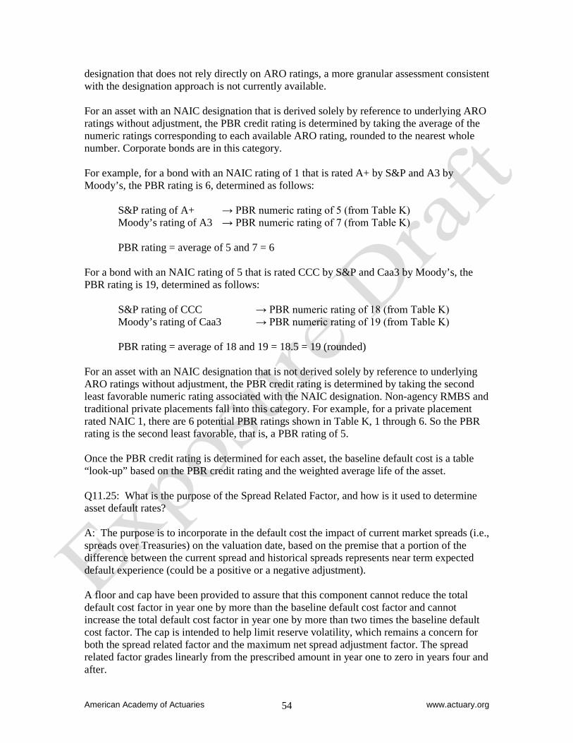
American Academy of Actuaries www.actuary.org 54
designation that does not rely directly on ARO ratings, a more granular assessment consistent with the designation approach is not currently available. For an asset with an NAIC designation that is derived solely by reference to underlying ARO ratings without adjustment, the PBR credit rating is determined by taking the average of the numeric ratings corresponding to each available ARO rating, rounded to the nearest whole number. Corporate bonds are in this category. For example, for a bond with an NAIC rating of 1 that is rated A+ by S&P and A3 by Moody’s, the PBR rating is 6, determined as follows:
S&P rating of A+ → PBR numeric rating of 5 (from Table K) Moody’s rating of A3 → PBR numeric rating of 7 (from Table K) PBR rating = average of 5 and 7 = 6
For a bond with an NAIC rating of 5 that is rated CCC by S&P and Caa3 by Moody’s, the PBR rating is 19, determined as follows:
S&P rating of CCC → PBR numeric rating of 18 (from Table K) Moody’s rating of Caa3 → PBR numeric rating of 19 (from Table K) PBR rating = average of 18 and 19 = 18.5 = 19 (rounded)
For an asset with an NAIC designation that is not derived solely by reference to underlying ARO ratings without adjustment, the PBR credit rating is determined by taking the second least favorable numeric rating associated with the NAIC designation. Non-agency RMBS and traditional private placements fall into this category. For example, for a private placement rated NAIC 1, there are 6 potential PBR ratings shown in Table K, 1 through 6. So the PBR rating is the second least favorable, that is, a PBR rating of 5. Once the PBR credit rating is determined for each asset, the baseline default cost is a table “look-up” based on the PBR credit rating and the weighted average life of the asset. Q11.25: What is the purpose of the Spread Related Factor, and how is it used to determine asset default rates? A: The purpose is to incorporate in the default cost the impact of current market spreads (i.e., spreads over Treasuries) on the valuation date, based on the premise that a portion of the difference between the current spread and historical spreads represents near term expected default experience (could be a positive or a negative adjustment). A floor and cap have been provided to assure that this component cannot reduce the total default cost factor in year one by more than the baseline default cost factor and cannot increase the total default cost factor in year one by more than two times the baseline default cost factor. The cap is intended to help limit reserve volatility, which remains a concern for both the spread related factor and the maximum net spread adjustment factor. The spread related factor grades linearly from the prescribed amount in year one to zero in years four and after.
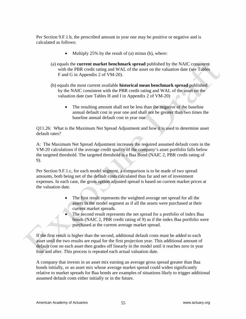
American Academy of Actuaries www.actuary.org 55
Per Section 9.F.1.b, the prescribed amount in year one may be positive or negative and is calculated as follows:
• Multiply 25% by the result of (a) minus (b), where:
(a) equals the current market benchmark spread published by the NAIC consistent with the PBR credit rating and WAL of the asset on the valuation date (see Tables F and G in Appendix 2 of VM-20).
(b) equals the most current available historical mean benchmark spread published
by the NAIC consistent with the PBR credit rating and WAL of the asset on the valuation date (see Tables H and I in Appendix 2 of VM-20)
• The resulting amount shall not be less than the negative of the baseline
annual default cost in year one and shall not be greater than two times the baseline annual default cost in year one.
Q11.26: What is the Maximum Net Spread Adjustment and how it is used to determine asset default rates? A: The Maximum Net Spread Adjustment increases the required assumed default costs in the VM-20 calculations if the average credit quality of the company’s asset portfolio falls below the targeted threshold. The targeted threshold is a Baa Bond (NAIC 2, PBR credit rating of 9). Per Section 9.F.1.c, for each model segment, a comparison is to be made of two spread amounts, both being net of the default costs calculated thus far and net of investment expenses. In each case, the gross option adjusted spread is based on current market prices at the valuation date.
• The first result represents the weighted average net spread for all the assets in the model segment as if all the assets were purchased at their current market spreads.
• The second result represents the net spread for a portfolio of index Baa bonds (NAIC 2, PBR credit rating of 9) as if the index Baa portfolio were purchased at the current average market spread.
If the first result is higher than the second, additional default costs must be added to each asset until the two results are equal for the first projection year. This additional amount of default cost on each asset then grades off linearly in the model until it reaches zero in year four and after. This process is repeated each actual valuation date. A company that invests in an asset mix earning an average gross spread greater than Baa bonds initially, or an asset mix whose average market spread could widen significantly relative to market spreads for Baa bonds are examples of situations likely to trigger additional assumed default costs either initially or in the future.
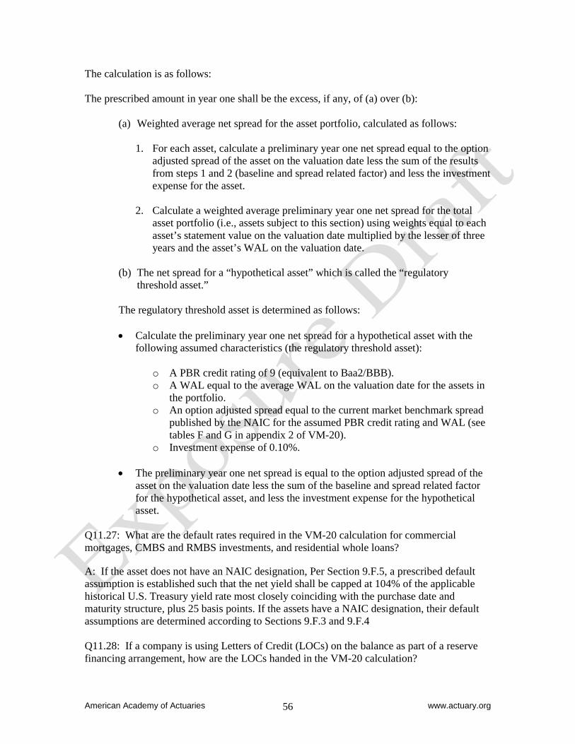
American Academy of Actuaries www.actuary.org 56
The calculation is as follows: The prescribed amount in year one shall be the excess, if any, of (a) over (b):
(a) Weighted average net spread for the asset portfolio, calculated as follows:
1. For each asset, calculate a preliminary year one net spread equal to the option adjusted spread of the asset on the valuation date less the sum of the results from steps 1 and 2 (baseline and spread related factor) and less the investment expense for the asset.
2. Calculate a weighted average preliminary year one net spread for the total
asset portfolio (i.e., assets subject to this section) using weights equal to each asset’s statement value on the valuation date multiplied by the lesser of three years and the asset’s WAL on the valuation date.
(b) The net spread for a “hypothetical asset” which is called the “regulatory
threshold asset.” The regulatory threshold asset is determined as follows:
• Calculate the preliminary year one net spread for a hypothetical asset with the
following assumed characteristics (the regulatory threshold asset):
o A PBR credit rating of 9 (equivalent to Baa2/BBB). o A WAL equal to the average WAL on the valuation date for the assets in
the portfolio. o An option adjusted spread equal to the current market benchmark spread
published by the NAIC for the assumed PBR credit rating and WAL (see tables F and G in appendix 2 of VM-20).
o Investment expense of 0.10%.
• The preliminary year one net spread is equal to the option adjusted spread of the asset on the valuation date less the sum of the baseline and spread related factor for the hypothetical asset, and less the investment expense for the hypothetical asset.
Q11.27: What are the default rates required in the VM-20 calculation for commercial mortgages, CMBS and RMBS investments, and residential whole loans? A: If the asset does not have an NAIC designation, Per Section 9.F.5, a prescribed default assumption is established such that the net yield shall be capped at 104% of the applicable historical U.S. Treasury yield rate most closely coinciding with the purchase date and maturity structure, plus 25 basis points. If the assets have a NAIC designation, their default assumptions are determined according to Sections 9.F.3 and 9.F.4 Q11.28: If a company is using Letters of Credit (LOCs) on the balance as part of a reserve financing arrangement, how are the LOCs handed in the VM-20 calculation?
American Academy of Actuaries www.actuary.org 57
A: Some actuaries will include LOCs in starting assets if the LOCs are treated as admitted assets on the balance sheet of the company. LOCs are typically admitted as an asset only if robust stress testing has indicated that a portion of the assets backing the total reserve are not needed to fund the obligations of the contract. This portion of the reserve is then backed by the LOC on the asset page. Since the LOC is backing the portion of the statutory reserve, some actuaries would conclude that it is appropriate to include the LOC in starting assets, even though the LOC is not an income producing asset.
In addition, some actuaries would also include the fee paid to the LOC provider as an expense in the future cash flows when performing the minimum reserve calculation, since it is an expense that is directly related to the underlying policy.
American Academy of Actuaries www.actuary.org 58
12. Details on Scenarios / Scenario Generators / Economic Assumptions Q12.1: What economic assumptions are stochastically generated? A: The prescribed scenario generator produces the following economic parameters:
1. Treasury rates at maturities of 0.25, 0.50, 1, 2, 3, 5, 7, 10, 20, and 30 years. (Filename: UST)
2. The following indices, with file names shown in parenthesis a. Aggressive or specialized equity (AGGR) b. Diversified international equity (INT) c. Diversified large cap US Equity (US) d. Intermediate risk equity (SMALL) e. Money market / Short term (MONEY) f. Intermediate term US government bond (INTGOV) g. US long term corporate bonds (LTCORP) h. Diversified fixed income (FIXED) i. Diversified balanced (BALANCED)
Treasury rates may be generated either as par bond, bond-equivalent (nominal semiannual) rates or as annual effective spot rates. Indices are total return indices, with one row for each scenario and one column for each time period. Actuaries may or may not choose to generate other measures stochastically, including inflation rates or currency exchange rates. Consideration should be given to the internal consistency of other stochastic quantities with the scenario data. Q12.2: How would actuaries generate the scenarios for the VM-20 calculations? A: Section 7.G.2 of VM-20 requires the actuary to use the “prescribed economic scenario generator with prescribed parameters” provided by the America Academy of Actuaries, with prescribed parameters. As of the date of this practice note, this generator, and the associated release notes and FAQ document, can be found at http://www.actuary.org/life/zip10/generator.zip and http://actuary.org/life/phase3.asp#10. The generator is updated periodically and users would be prudent to verify they have the current version of the generator. Similarly, Section 7.G.1 requires using the same tool to generate the scenario used in to determine the deterministic reserves, and Section 6.A.2.a requires using this tool to generate the stochastic exclusion test scenarios. Note, some actuaries may believe that using the “prescribed economic scenario generator with prescribed parameters” means using the specific provided Excel workbook. However, other actuaries might reasonably conclude that any other tool that would generate the same results, using the same formulas and parameters, would also be acceptable. Q12.3: How many Scenarios should be run to determine the Stochastic Reserve?
American Academy of Actuaries www.actuary.org 59
A: The current version of VM-20 does not define the appropriate number of scenarios to run. The prescribed scenario generator allows the user to choose the “full set of 10,000 scenarios,” as well as subsets of 1,000, 500, 200, and 50 scenarios. From this, some actuaries would run all 10,000 scenarios to meet the regulatory requirements under VM-20. Some actuaries would use less than the 10,000 scenarios. Various methods are available for determining the adequacy of the size of a scenario set. Some actuaries may test convergence by running all 10,000 scenarios, and then test to see what reserve would be calculated with the first 1,000, then the first 2,000, the first 3,000, and so on. If this series converges rapidly, the actuary could use a smaller subset that based on actuarial judgment is sufficient. The actuary might conclude that it is necessary to repeat this test only when the characteristics of the liabilities, the assets backing them, or the economic environment have materially changed. Q12.4: How would the actuary determine the appropriate number of scenarios if less than the full 10,000 scenario set is used? A: A range of methods might be appropriate to pick such a subset of n scenarios, including, but not limited to, the following:
• Using the scenario picker embedded in the prescribed generator or • Selecting the first n scenarios, or some random subset of the scenarios, or • Using an alternative scenario picking or reduction tool.
The actuary may wish to use caution in using the scenario picker, as it relies on only the 20 year Treasury rate as the driver of scenario selection. Thus, for products that are sensitive to equity performance or other maturities, the scenario picker may not be an effective scenario reduction technique. Section 7.G.2 indicates that scenario reduction techniques may be considered acceptable as long as:
i. the smaller set of scenarios are chosen from the larger set of scenarios
prescribed by the NAIC; ii. the scenario reserves of a representative subset of policies, run using the
reduced scenario set, are consistent with the scenario reserves of the same subset of policies, run using the larger scenario set; and
iii. use of the full set of scenarios would not result in a materially greater reserve.
Some actuaries might conclude that a “representative subset” could mean a highly compressed model of the in force business, or it might mean a random sample of the in force. An actuary may conclude that a model is “representative” if it would produce a similar reserve to what the entire in force would produce if run across a small subset of the scenarios. Thus, for example, an actuary might:
American Academy of Actuaries www.actuary.org 60
• Tentatively select a subset of the scenarios. • Calculate reserves across these scenarios using a tentatively selected subset of the
liabilities and using the entire inforce business. If these results are similar, then the actuary might reasonably conclude that the subset of the liabilities is appropriate to use to measure the appropriateness of a scenario subset.
• Calculate reserves for the subset of the liabilities across both the reduced set of scenarios and the full set of scenarios. If the reserves calculated for the subset of liabilities using the scenario subset are not materially smaller than the reserves calculated for the subset of liabilities using all the scenarios, then the actuary might reasonably conclude that the subset of scenarios is appropriate to use.
In addition, some actuaries might conclude that if the same technique is used to pick a representative subset of the liabilities in successive periods, then it is not necessary to revalidate the appropriateness of that liability subset for use in validating scenario subsets. For randomly selected subsets, one commonly accepted method was published by Manistre and Hancock (Manistre and Hancock, Variance of the CTE Estimator, NAAJ, Vol 9, No.2 (April 2005), pages 129-156.). However it is important to understand that this test is appropriate only when using randomly selected subsets of a pool of scenarios. It is not an appropriate technique to use for intelligent scenario compression techniques or when using the scenario picking tool. Q12.5: What if there are a lower number of scenarios that results in a higher reserve than a greater number of scenarios? A: VM-20 does not prevent the actuary from selecting a scenario subset that produces a reserve that is greater than what would result if the full set is used. Some actuaries would hold the lower reserve based on the larger number of scenarios to take into account the additional credibility of the larger scenario set. Other actuaries would hold the higher reserve based on the smaller scenario set (if in the actuary’s judgment the number of scenarios in the smaller scenario set is reasonable for the purpose of calculating the Stochastic Reserve requirement). Q12.6: Can the actuary use scenarios other than prescribed scenarios for calculating the Stochastic Reserve. A: Section 7.G.2 specifically requires use of the “prescribed economic scenario generator with prescribed parameters.” Q12.7: How are separate account funds mapped into specific equity index Scenarios? A: Section 7.G.2 states that:
Mapping of the returns on the proxy funds to the prescribed fund’s returns is left to the judgment of the actuary, but the returns so generated must be consistent with the prescribed returns. This does not imply a strict functional relationship between the model parameters for various markets/funds, but it would generally be inappropriate to assume that a market or
American Academy of Actuaries www.actuary.org 61
fund consistently “outperforms” (lower risk, higher expected return relative to the efficient frontier) over the long term. Actuaries might wish to effect modeling of funds in different ways. For example, one reasonable way might be to perform a regression of past fund performance against past performance of market indices consistent with the scenario generator classifications, and develop a scenario set for each such fund that is consistent with an appropriate weight of such scenarios derived from the regression. Alternatively, funds might be decomposed using regression techniques into funds corresponding to each of the indices. Q12.8: How can the actuary obtain the scenarios used for the stochastic exclusion test? A: The same prescribed generator used for stochastic scenario generation should be used to generate the 16 scenarios used for the stochastic exclusion test. Q12.9: How can the actuary obtain the scenario used for the Deterministic Reserve? A: The Deterministic Reserve is to be calculated using scenario 12 from the set of stochastic exclusion test scenarios. Q12.10: What changes should be made to the prescribed stochastic scenario generator parameters for non-US economies? A: Section 7.G.2 requires the actuary to use the approved scenario generator provided by the American Academy of Actuaries, with prescribed parameters. That said, some actuaries might conclude that it is unreasonable to use these parameters for non-U.S. interest rates. In a situation where non-U.S. interest rates are required, some actuaries would deem it appropriate to:
• Use historical interest rates in that market, in the same formula used in the U.S., to determine the mean reversion target appropriate for that market, and
• Update the starting yield curve to match government bond yields in that market. In addition, some actuaries might wish to update volatility, correlation, and other parameters to be consistent with the market in question. For equity returns in non-U.S. markets, the actuary might want to use techniques similar to what is used for U.S. funds to map each fund into one or more of the funds generated by the prescribed generator. A guidance note in this section after 7.G.2.b states that it would generally be inappropriate to assume that a market or fund consistently outperforms (lower risk, higher expected return relative to the efficient frontier) over the long term. Q12.11: How should the actuary generate interest rates for maturities not generated by the economic scenario generator?
American Academy of Actuaries www.actuary.org 62
A: The prescribed scenario generator only generates interest rates for selected terms to maturity. For some purposes, the actuary might have need of a full set of interest rates at other maturities. A range of options are available for this. VM-20 gives no guidance. Techniques some actuaries might find reasonable could include, but would not be limited to, the following:
• Linear interpolation, or • Bootstrapping the curve to find forward rates that increase linearly between the given
maturity points and are consistent with the given rates, or • Using the Nelson-Siegel parameters and formulas documented in the scenario
generator release notes, or • Cubic spline interpolation.
American Academy of Actuaries www.actuary.org 63
13. Setting Prudent Estimate and Anticipated Experience Assumptions Q13.1: How are prudent estimate assumptions determined? A: VM-20, Section 1 defines margins and prudent estimate assumptions where prudent estimate assumptions equal anticipated experience assumptions plus a margin. The margin may increase or decrease the assumption as appropriate to cover adverse deviations and estimation error. The margin should result in a larger reserve than would otherwise result without it. There is no requirement in VM-20 to add a margin to assumptions that are stochastically modeled because the applicable CTE measure provides a margin. Some actuaries will set a prudent estimate assumption without separately determining an anticipated experience assumption and a margin. An example of this could be if the sensitivity testing shows that the risk factor does not have a material impact on the reserve. Another example could be that the actuary believes the assumption includes enough of a margin even if the margin is not explicitly determined separately. It would be good practice to review the relevant Actuarial Standards of Practice including but not limited to: No. 2 Nonguaranteed Charges or Benefits for Life Insurance Policies and Annuity Contracts No. 7 Analysis of Life, Health, or Property/Casualty Insurer Cash Flows No. 11 Treatment of Reinsurance Transactions Involving Life or Health Insurance No. 22 Statements of Opinion Based on Asset Adequacy Analysis by Actuaries for Life and Health Insurers No. 23 Data Quality The Actuarial Standards Board is developing a new ASOP, Standards for Principle-Based Reserves for Life Products that the actuary likely will wish to also consider. Q13.2: Are the same prudent estimate assumptions used for deterministic and stochastic calculations? A: Section 9.A.5 requires prudent estimate assumptions to be consistent for the two calculations. Some actuaries would use the same assumptions except where the risk factor is scenario dependent. Q13.3: Which risk factors do not require a prudent estimate assumption? A: According to Sections 9.A.3 and 9.A.4, the company is not required to develop prudent estimates for assumptions that are prescribed, or stochastically modeled such as interest rate movements (i.e., Treasury interest rate curves) and equity performance or any other assumption that is stochastically modeled. Some actuaries might not develop a prudent estimate assumption for risk factors that do not materially affect the cash flows of the product or the reserve as permitted by Section 7.A.2. Q13.4: How will actuaries set anticipated experience assumptions?
American Academy of Actuaries www.actuary.org 64
A: Per VM-20, Section 9.A.6, the actuary shall use company experience, if relevant and credible, to establish the anticipated experience assumption for any risk factor. To the extent the company experience is not available or credible, the actuary may use industry experience or other data to establish the anticipated experience assumption, making modifications as needed to reflect the actuary’s expectation of the risk. Some actuaries may develop anticipated experience assumptions based on the assumptions used for pricing and development of the product. Those actuaries may wish to consider whether it is necessary to work closely with the product development actuary to understand the basis for assumptions and review the studies performed prior to using them in the reserve calculations to assure they meet the criteria set in Section 9.A.6. Q13.5: Can actuaries use company experience if it predates the effective date of VM-20? A: Some actuaries will use company experience that predates the effective date of VM-20 if it is relevant and credible for the assumption or margin that is being determined. There is no requirement in VM-20 that the experience data used to determine anticipated experience and/or margins for prudent estimate assumptions has to be after the effective date of VM-20. Q13.6: When would the actuary update the anticipated experience assumptions? A: Section 9.A.6 requires the actuary to annually review relevant emerging experience and Section 9.A.2 requires that the assumptions be periodically reviewed and updated. Therefore, it is expected that actuaries will update assumptions if there is new experience data or other information that changes the actuary’s expectation of future experience. Actuaries will use materiality, company practice for updating assumptions and the credibility of the new data and other information in determining whether or not to update the experience assumptions. Experience assumptions are not locked in at issue. Q13.7: What data sources may be used to set anticipated experience assumptions? A: Some actuaries would first look to company specific data, if relevant and credible, to set anticipated experience assumptions. However, in instances where company specific data is not available or credible, actuaries may wish to consider looking to alternative sources as discussed in Section 9.A.6.b. A non-exhaustive list of possible data sources to consider for developing anticipated experience assumptions are listed below:
• Company data on the same or similar products • Industry or reinsurer data on the same or similar products • General population data • Predictive models or algorithms
For assumptions that are established based on limited data, Section 9.A.6.d. requires the actuary to sensitivity test the assumption chosen to ensure the assumption is set at the conservative end of the plausible range.
American Academy of Actuaries www.actuary.org 65
Q13.8: What other issues should the actuary take into account when setting anticipated experience assumptions? A: The actuary may wish to consider whether anticipated experience assumptions developed from the data should be modified as needed to reflect the circumstances of the company. For example, if the data from alternative sources includes mortality experience based on three underwriting classes, and the company has just two underwriting classes, then adjustments to the assumptions may be needed to make them appropriate for the company’s underwriting classes. The actuary may wish to consider adjusting assumptions based on historical experience to consider those guarantees that are available in the contracts that were not materially prevalent in the experience base. The actuary may also wish to consider the possibility of anti-selection affecting assumptions. For example, anti-selection may involve a combination of lapses, persistency, mortality, and the level of guarantees. The actuary may also wish to consider reviewing guarantees related to cash inflows and outflows to determine to what degree these future cash flows may be incorporated in the model. The actuary may wish to consider the probability of events occurring that may materially impact future assumptions. Q13.9: When might it be appropriate to represent extreme or catastrophic behavior? A: Section 9.D.2.c states that the company is not required to model extreme or “catastrophic” forms of behavior in the absence of evidence to the contrary. Some actuaries would reflect extreme or catastrophic behavior if it is evidenced by recent historical experience and is consistent with the anticipated experience. Q13.10: How should trends in data affect the anticipated experience assumption? A: Some actuaries would use the smallest breakdown of data that is available and credible over time for comparison to experience of other exposure periods. However, judgment is needed here as the actuary has to balance precision against credibility considering the practical ability to do the necessary studies. An example would be in analyzing lapse data for a certain product over calendar years 2000-2004 to the same grouping over calendar years 2005-2009. Some actuaries would project trends that in their judgment are likely to be sustained in the future in the anticipated experience assumption, subject to any applicable restrictions. Some actuaries would make a judgment on the uncertainly surrounding the projection of the trend and increase the margin as uncertainty increases, such as in later durations. Q13.11: How does the actuary determine if company experience data is credible? A: A discussion of credibility in the context of the mortality assumption is found in Section 15 of this practice note. To make a determination on the level of credibility that a set of company experience may have, some actuaries will use concepts from classical credibility theory. In this sense, the actuary may determine that full credibility will be established when
American Academy of Actuaries www.actuary.org 66
enough observations of an event occur so that the actual result of its frequency will be within a defined percentage of the expected results with a specified probability. Additional adjustments to the definition of full credibility may be used in cases where the actual observed events can range in their magnitude of severity. The actuary may wish to review the Credibility Practice Note which can be found on the American Academy of Actuaries website at www.actuary.org. If the number of observations is fewer than the amount needed for full credibility, partial credibility of the data may be established. This can be done by using information such as the expected number of observations and the number of observations needed for full credibility. Some actuaries with data that is only partially credible will use actuarial judgment to combine partially credible data with other industry experience to determine their anticipated experience assumptions. Q13.12: Should the actuary perform sensitivity testing to set anticipated experience assumptions? A: Section 9.A.7 requires sensitivity testing to understand the materiality of prudent estimate assumptions on the minimum reserve. Some actuaries would perform the sensitivity testing using anticipated experience assumptions. Other actuaries would instead perform the sensitivity testing using prudent estimate assumptions. If the sensitivity testing shows that the assumption is material to the minimum reserve level, Section 9.B.3 says that greater analysis and more detailed justification are needed to determine the level of uncertainty when establishing margins for risk factors that produce greater sensitivity on the modeled reserve. Therefore, it may be prudent for the actuary to review the credibility of the data used to set the assumption and if the assumption is set at the appropriate level.
American Academy of Actuaries www.actuary.org 67
14. Setting Margins Q14.1: What are the VM-20 requirements when determining appropriate margins? A: Section 9.B states that assumptions that are neither stochastically determined nor prescribed should incorporate appropriate margins for adverse deviation and estimation error. The actuary is required to set an explicit margin for each material assumption independently but, if applicable, the actuary may apply a covariance adjustment when certain requirements are met. A margin is not required for assumptions that have an immaterial impact on the minimum reserve. Section 9.B.2 states that higher margins should be used when:
• The experience data have less relevance or lower credibility; • The experience data are of lower quality, such as incomplete, internally inconsistent,
or not current; • There is doubt about the reliability of the anticipated experience assumption, such as,
but not limited to recent changes in circumstances or changes in company policies; or • There are constraints in the modeling that limit an effective reflection of the risk
factor Greater analysis and more detailed justification are required when establishing margins for risk factors that produce greater sensitivity of the minimum reserve. Section 9.B.5 states that in setting the margin for a risk factor, the actuary must consider the magnitude of fluctuations in historical experience of the company for that risk factor, as appropriate. Section 9.B.6 states that the company shall apply the method used to determine the margin consistently on each valuation date, but is permitted to change the method from the prior year if the rationale for the change and the impact on modeled reserve is disclosed. Sections 9.C.5, and 9.D.3 provide specific requirements for setting margins for mortality and policyholder behavior respectively. Q14.2: What other references are available when determining appropriate margins? A: Some actuaries may look to the following:
• SOA Research Paper titled Analysis of Methods for Determining Margins for Uncertainty Under a Principle-Based Framework for Life Insurance and Annuity Products (March 31, 2009).
• Draft ASB ASOP titled, Standards for Principle-Based Reserves for Life Products • The C3 Phase 3 Report and associated Practice Note. • The AG-43 / C3 Phase II Practice Note. • Internal documentation of margins used for other financial reporting methods, for
example, US GAAP FAS 60 margins. • Various Canadian VTPs (Valuation Technique Papers) and educational notes
American Academy of Actuaries www.actuary.org 68
Q14.3: What general method should be used in setting margins? A: Some actuaries will focus on the key assumptions for the underlying product first and then analyze how those margins affect other assumptions. For example, for an annually renewable term product, the actuary may initially focus on setting the mortality anticipated experience and margin assumptions (since it is a principal risk) and then set other assumptions such as lapse rates and expenses such that these assumptions are internally consistent with the mortality assumption. One advantage of concentrating on the key assumptions is avoiding the situation where the application of a margin to one assumption affects the direction of the appropriate margin to apply to another assumption (e.g., a high mortality margin may cause lower rather than higher lapses to be conservative). Some actuaries would develop an approach to setting margins in a manner consistent with the underlying principle of reflecting the underlying risk characteristics of the product. Q14.4: When can and how does the actuary apply a covariance adjustment in setting the margins? A: Per Section 9.B.1, the initial level of a particular margin may be adjusted to take into account the fact that risk factors are not normally 100% correlated. The initially determined margin may only be reduced to the extent the company can demonstrate that the method used to justify such a reduction is reasonable considering the range of scenarios contributing to the CTE calculation, recognizing that risk factors may become more correlated in adverse circumstances, or considering the scenario used to calculate the Deterministic Reserve as applicable or considering appropriate adverse circumstances for risk factors not stochastically modeled. Industry practice determining covariance adjustments is expected to evolve over time. Q14.5: Does the sensitivity of an assumption’s impact on the overall reserve level affect how the margin is set? A: In setting the margins in the calculation Section 9.B.5 states that the actuary must consider the magnitude of fluctuation in the historical experience of the company for the risk factor. One approach to determining the uncertainty of a risk factor, is to measure the standard deviation around the mean or other standard statistical measure (if meaningful historical experience data are available for the risk factor). Section 9.B.2 lists some considerations that would lead to a larger margin. They are when:
• The experience data have less relevance or lower credibility. • The experience data are of lower quality, such as incomplete, internally inconsistent,
or not current. • There is doubt about the reliability of the anticipated experience assumption, such as,
but not limited to, recent changes in circumstances or changes in company policies.
American Academy of Actuaries www.actuary.org 69
• There are constraints in the modeling that limit an effective reflection of the risk factor.
Some actuaries will not include a larger margin for risk factors with material impact on the reserves but little uncertainty. For example, if an expense assumption has a large impact on the reserve but is known with certainty (has been outsourced for a fixed contractual cost), then a smaller margin could be appropriate. Q14.6: What are the types of uncertainty that need to be considered when establishing the margin for a risk factor? A: Section 9.B requires the consideration of mis-estimation of the underlying distribution and random fluctuation around the mean of that distribution. Some actuaries would use Monte-Carlo simulation as a means of analyzing the random fluctuation for some risk factors. Other methodologies likely will be used such as identifying a likely range of expected outcomes and setting margins based on the range. Q14.7: Are there additional considerations for setting margins for specific assumptions? A: The specific considerations for mortality, policyholder behavior and expense margins are discussed in the respective sections of this practice note covering those items. Q14.8: Can the actuary use Canadian prescribed margins? A: Some actuaries may use Canadian prescribed margins, but VM-20 does not list them as a “safe harbor.” The actuary would need to make a determination of their appropriateness for use in the reserve calculation as set forth in VM-20. Q14.9: To what extent should the size of the company affect the size of the margins used? A: Some actuaries would not modify the size of the margins based solely on the size of the company. For example, larger margins should generally coincide with a reduction in uncertainty that might be due to a large number of observations, but is not necessarily dependent on company size since a large number of observations could be generated over time from a smaller company. Q14.10: What are the considerations for setting margins across blocks of business? A: Some actuaries would assess whether the margins were appropriate by product as well as adequate over a broad set of policies. This assessment would be particularly useful for products with uncertain risks or particularly unique characteristics. It is expected that some actuaries would review the margins in aggregate, particularly where policy characteristics are similar or have homogeneous risks. Q14.12: How should margins be set when the impact of assumption movements changes over the duration of the business?
American Academy of Actuaries www.actuary.org 70
A: For some products, the impact on the overall reserve of increasing or decreasing an assumption may vary according to the duration of the business. Since margins are intended to add conservatism, in the case where the impact of the margins varies by duration, some actuaries would set margins that change based on duration. However, some actuaries would set a specific margin on an assumption that complies with Section 9.B requirements overall even if there may be some durations where the margin decreases the reserve. In other words, the margin increases the overall reserve but may not increase it in every duration. Where there is a clear change in the policy, such as a dramatic change in premiums or surrender charges, some actuaries will develop margins that differ before and after this point. Q14.13: How are margins determined for dynamic assumptions? A: As implied by Sections 9.A.3 and 9.A.4, where an assumption is interest rate or equity return dependent, and a dynamic formula is included in the modeling, some actuaries may not add an additional margin to the calculation, on the basis that conservatism is provided by the conservatism inherent in the tail measure (i.e., CTE) and in their judgment this implicit margin would satisfy the requirements of Section 9.B. However, other actuaries may add additional conservatism, as they might feel that the use of the tail measure will only inject conservatism regarding the interest rate or equity risk, but not necessarily the dynamically related risk, which they may see as a distinct risk. Some of these actuaries might add conservatism by making the dynamic formula slightly more or less dynamic (depending on what would be more conservative) than anticipated. Some actuaries might consider margins on the base underlying assumption to be applicable to the resulting assumption including dynamic components, so would not add an additional margin. Q14.14: How often should margins be updated? A: Some actuaries would use consistent margins or the same margins from one reporting date to the next unless there is a particular reason the actuary believes the credibility, quality or reliability of the assumption has changed. Other actuaries may review and update margins, where necessary, on a regular basis every time they perform the calculation.
American Academy of Actuaries www.actuary.org 71
15. Setting Mortality Assumptions Q15.1: What are the steps to determining mortality assumptions for the Deterministic Reserve and/or Stochastic Reserve? A: For these reserves, mortality assumptions are discussed in Section 9.C. of VM-20. (For the Net Premium Reserve, mortality assumptions are provided in Section 3.C.1.) The following approach is defined for determining the prudent estimate mortality assumption:
1. Determine mortality segments (Section 9.C.1.a). 2. Determine company experience rates as provided in Section 9.C.2, or, if company
experience data is limited or not available, use an applicable industry basic table or other applicable experience in lieu of company experience as provided in Section 9.C.3.
3. If the company determines company experience mortality rates as provided in Section 9.C.2, then use the procedure described in Section 9.C.3 to determine the applicable industry table for each mortality segment to grade company experience to the industry table. If the company is using an applicable industry basic table in lieu of company experience as provided in Section 9.C.3, skip to step 5.
4. Determine the level of credibility of the underlying company experience as provided in Section 9.C.4. Per subsection 9.C.4.b, credibility may be determined at either the mortality segment level or at a more aggregate level if the mortality for the sub-classes was determined using an aggregate level of mortality experience.
5. Determine the prescribed mortality margins as provided in Section 9.C.5. Separate mortality margins are determined for company experience mortality rates and the applicable industry basic tables. Prescribed margin percentages shall be increased, as appropriate, to reflect the level of uncertainty related to situations, including, but not limited to, those described in Section 9.C.5.d.
6. Use the procedure described in Section 9.C.6 to determine the prudent estimate anticipated experience.
Q15.2: Is the company required to determine its own company experience mortality rates, or can it just use an industry mortality table? A: Section 9.C.1.b.i. states that the company can use an industry table for mortality if the company experience data is limited or not available. Some actuaries interpret Section 9.C.6.a to allow the company to use industry mortality tables, instead of company’s mortality experience. However, Section 9.C.6.biii states that “if the credibility of company’s data is less than 10%, the company cannot use their own experience, industry tables should be used instead.” Q15.3: Should the mortality rates be based on experience for each cell, for each mortality segment, or for the company? A: Section 9.C.2.b states that company experience data shall be based on experience from the following sources:
i. Actual company experience for books of business within the mortality segment.
American Academy of Actuaries www.actuary.org 72
ii. Experience from other books of business within the company with similar underwriting.
iii. Experience data from other sources, if available and appropriate, such as actual experience data of one or more mortality pools in which the policies participate under the term of a reinsurance agreement. Data from other sources is appropriate if the source has underwriting and expected mortality experience characteristics that are similar to policies in the mortality segment.
VM-20 states that company experience mortality rates shall be determined for each mortality segment (Section 9.C.2.a), but the rates can be based on more aggregate experience (Section 9.C.2.d). If experience is aggregated, Section 9.C.2.d states that the company should use other techniques to further subdivide the aggregate class into various sub-classes or mortality segments. In doing so, the company must ensure that when the mortality segments are weighted together, the total number of expected claims is not less than the company experience data for the aggregate class. Q15.4: How should the mortality rates that were established based on the aggregate company experience be subdivided into sub-classes (mortality segments)? A: VM-20 does not specify a method for subdividing aggregate company experience into sub-classes or mortality segments. However, Section 9.C.2.d does state that the company must ensure that when the mortality segments are weighted together, the total number of expected claims is not less than the company experience data for the aggregate class. Some actuaries would use the Conservation of Total Deaths and / or the Preservation of Deaths methods to subdivide aggregate mortality rates into sub-classes. Other approaches may be acceptable. Please see the following source documents for more information on each method. Conservation of Deaths SOA Study Note ILA-D107--07, Experience Assumptions for Individual Life Insurance and Annuities by Lambert, Page 25. Preservation of Total Deaths Life Insurance Products and Finance by Atkinson and Dallas, Section 3.2.4.3 "Effect of Selective Lapses", Pages 149-151 Q15.5: How long of an exposure period should be used in the experience study used to determine the mortality assumptions? A: Section 9.C.2.e.ii states that that the exposure period for the mortality experience study should be at least three exposure years, but no more than 10 exposure years. Q15.6: How often do experience studies need to be updated?
American Academy of Actuaries www.actuary.org 73
A: Section 9.C.2.e indicates that the company shall review the mortality experience (in a credibility segment) at least once every three years and update as needed. Some companies may review their experience every year, while others may establish a rotating basis for annual reviews of experience across credibility segments so that each segment is reviewed at least every three years. Some companies may leverage experience studies that are being performed for other purposes within the company, or the experience reporting for VM-51 and perform reviews at that time. Section 9.C.2.e indicates that the company shall reflect changes implied by the updated data to the extent that such changes are significant and are expected to continue into the future. Q15.7: Can mortality improvement be used? A: Section 9.C.2.h indicates that the company may reflect mortality improvement from the central point of the underlying company experience data to the valuation date. The mortality rates from the applicable industry basic table may be improved from the year of the table to the valuation date, as indicated in Section 9.C.3.g. The company is prohibited by VM-20 from reflecting mortality improvement beyond the projection date. Some actuaries would use published mortality improvement rates to incorporate mortality improvement into the company experience mortality rates and update the improvement factors every year. Other actuaries may only update the projected improvement factors in conjunction with the review of underlying experience and updates of the experience mortality. Actuaries may use improvement factors for the applicable industry table, applied to the industry table, that will be determined and published by the Society of Actuaries (SOA). Q15.8: Would the actuary need to use a specific credibility method to determine the credibility of the mortality experience used to develop the mortality assumption? A: VM-20 does not mandate a particular credibility method. Methods such as Limited Fluctuation, Greatest Accuracy or other statistical approaches such as the Panjer method are approaches that could be used to determine credibility of mortality experience. Another resource on credibility methods is the American Academy of Actuaries Credibility Practice Note. The Society of Actuaries Research Department also published a paper “Credibility Theory Practices” that can be found at http://www.soa.org/files/pdf/research-cred-theory-pract.pdf, and the Canadian Institute of Actuaries has also published the Expected Mortality Educational Note at https://www.actuaries.ca/educational_notes/ed_notes_e.cfm. Q15.9: How would the actuary determine if company mortality experience data is credible? A: Subsection 9.C.4, provides the requirements for the credibility calculation:
1. For valuations prior to January 1, 2015, the methodology must follow common actuarial practice as published in actuarial literature (for example but not limited to the Limited Fluctuation Method or Panjer method).
2. For valuations after January 1, 2015, there is an additional requirement that the level of credibility over the entire exposure period shall be determined such that the minimum probability is at least 95% with an error margin of no more than 5%.
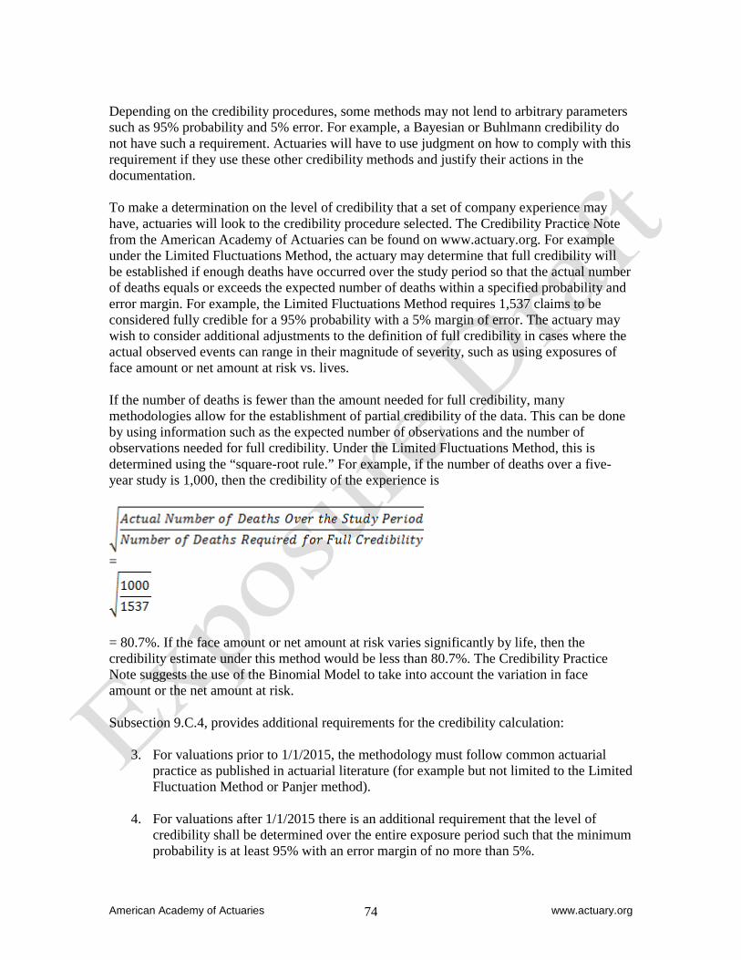
American Academy of Actuaries www.actuary.org 74
Depending on the credibility procedures, some methods may not lend to arbitrary parameters such as 95% probability and 5% error. For example, a Bayesian or Buhlmann credibility do not have such a requirement. Actuaries will have to use judgment on how to comply with this requirement if they use these other credibility methods and justify their actions in the documentation. To make a determination on the level of credibility that a set of company experience may have, actuaries will look to the credibility procedure selected. The Credibility Practice Note from the American Academy of Actuaries can be found on www.actuary.org. For example under the Limited Fluctuations Method, the actuary may determine that full credibility will be established if enough deaths have occurred over the study period so that the actual number of deaths equals or exceeds the expected number of deaths within a specified probability and error margin. For example, the Limited Fluctuations Method requires 1,537 claims to be considered fully credible for a 95% probability with a 5% margin of error. The actuary may wish to consider additional adjustments to the definition of full credibility in cases where the actual observed events can range in their magnitude of severity, such as using exposures of face amount or net amount at risk vs. lives. If the number of deaths is fewer than the amount needed for full credibility, many methodologies allow for the establishment of partial credibility of the data. This can be done by using information such as the expected number of observations and the number of observations needed for full credibility. Under the Limited Fluctuations Method, this is determined using the “square-root rule.” For example, if the number of deaths over a five-year study is 1,000, then the credibility of the experience is
=
= 80.7%. If the face amount or net amount at risk varies significantly by life, then the credibility estimate under this method would be less than 80.7%. The Credibility Practice Note suggests the use of the Binomial Model to take into account the variation in face amount or the net amount at risk. Subsection 9.C.4, provides additional requirements for the credibility calculation:
3. For valuations prior to 1/1/2015, the methodology must follow common actuarial practice as published in actuarial literature (for example but not limited to the Limited Fluctuation Method or Panjer method).
4. For valuations after 1/1/2015 there is an additional requirement that the level of credibility shall be determined over the entire exposure period such that the minimum probability is at least 95% with an error margin of no more than 5%.
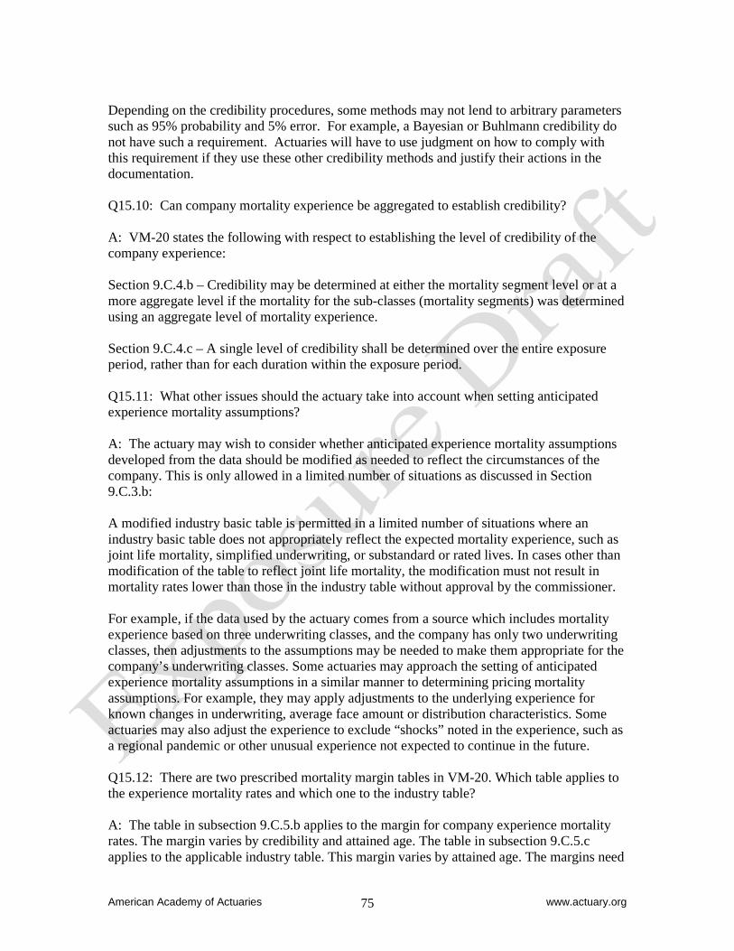
American Academy of Actuaries www.actuary.org 75
Depending on the credibility procedures, some methods may not lend to arbitrary parameters such as 95% probability and 5% error. For example, a Bayesian or Buhlmann credibility do not have such a requirement. Actuaries will have to use judgment on how to comply with this requirement if they use these other credibility methods and justify their actions in the documentation. Q15.10: Can company mortality experience be aggregated to establish credibility? A: VM-20 states the following with respect to establishing the level of credibility of the company experience: Section 9.C.4.b – Credibility may be determined at either the mortality segment level or at a more aggregate level if the mortality for the sub-classes (mortality segments) was determined using an aggregate level of mortality experience. Section 9.C.4.c – A single level of credibility shall be determined over the entire exposure period, rather than for each duration within the exposure period. Q15.11: What other issues should the actuary take into account when setting anticipated experience mortality assumptions? A: The actuary may wish to consider whether anticipated experience mortality assumptions developed from the data should be modified as needed to reflect the circumstances of the company. This is only allowed in a limited number of situations as discussed in Section 9.C.3.b: A modified industry basic table is permitted in a limited number of situations where an industry basic table does not appropriately reflect the expected mortality experience, such as joint life mortality, simplified underwriting, or substandard or rated lives. In cases other than modification of the table to reflect joint life mortality, the modification must not result in mortality rates lower than those in the industry table without approval by the commissioner. For example, if the data used by the actuary comes from a source which includes mortality experience based on three underwriting classes, and the company has only two underwriting classes, then adjustments to the assumptions may be needed to make them appropriate for the company’s underwriting classes. Some actuaries may approach the setting of anticipated experience mortality assumptions in a similar manner to determining pricing mortality assumptions. For example, they may apply adjustments to the underlying experience for known changes in underwriting, average face amount or distribution characteristics. Some actuaries may also adjust the experience to exclude “shocks” noted in the experience, such as a regional pandemic or other unusual experience not expected to continue in the future. Q15.12: There are two prescribed mortality margin tables in VM-20. Which table applies to the experience mortality rates and which one to the industry table? A: The table in subsection 9.C.5.b applies to the margin for company experience mortality rates. The margin varies by credibility and attained age. The table in subsection 9.C.5.c applies to the applicable industry table. This margin varies by attained age. The margins need
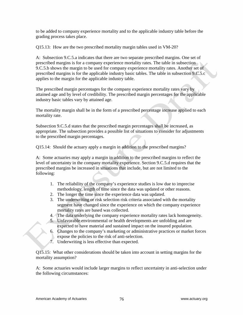
American Academy of Actuaries www.actuary.org 76
to be added to company experience mortality and to the applicable industry table before the grading process takes place. Q15.13: How are the two prescribed mortality margin tables used in VM-20? A: Subsection 9.C.5.a indicates that there are two separate prescribed margins. One set of prescribed margins is for a company experience mortality rates. The table in subsection 9.C.5.b shows the margin to be used for company experience mortality rates. Another set of prescribed margins is for the applicable industry basic tables. The table in subsection 9.C.5.c applies to the margin for the applicable industry table. The prescribed margin percentages for the company experience mortality rates vary by attained age and by level of credibility. The prescribed margin percentages for the applicable industry basic tables vary by attained age. The mortality margin shall be in the form of a prescribed percentage increase applied to each mortality rate. Subsection 9.C.5.d states that the prescribed margin percentages shall be increased, as appropriate. The subsection provides a possible list of situations to consider for adjustments to the prescribed margin percentages. Q15.14: Should the actuary apply a margin in addition to the prescribed margins? A: Some actuaries may apply a margin in addition to the prescribed margins to reflect the level of uncertainty in the company mortality experience. Section 9.C.5.d requires that the prescribed margins be increased in situations that include, but are not limited to the following:
1. The reliability of the company’s experience studies is low due to imprecise methodology, length of time since the data was updated or other reasons.
2. The longer the time since the experience data was updated. 3. The underwriting or risk selection risk criteria associated with the mortality
segment have changed since the experience on which the company experience mortality rates are based was collected.
4. The data underlying the company experience mortality rates lack homogeneity. 5. Unfavorable environmental or health developments are unfolding and are
expected to have material and sustained impact on the insured population. 6. Changes to the company’s marketing or administrative practices or market forces
expose the policies to the risk of anti-selection. 7. Underwriting is less effective than expected.
Q15.15: What other considerations should be taken into account in setting margins for the mortality assumption? A: Some actuaries would include larger margins to reflect uncertainty in anti-selection under the following circumstances:
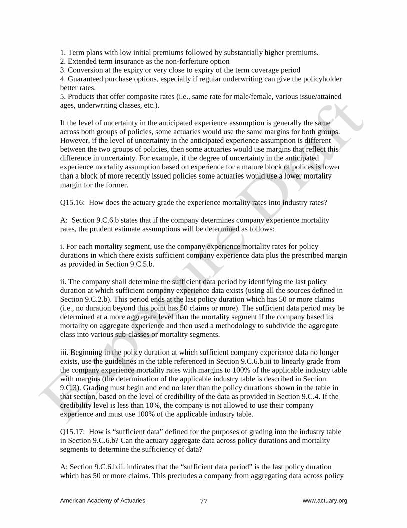
American Academy of Actuaries www.actuary.org 77
1. Term plans with low initial premiums followed by substantially higher premiums. 2. Extended term insurance as the non-forfeiture option 3. Conversion at the expiry or very close to expiry of the term coverage period 4. Guaranteed purchase options, especially if regular underwriting can give the policyholder better rates. 5. Products that offer composite rates (i.e., same rate for male/female, various issue/attained ages, underwriting classes, etc.). If the level of uncertainty in the anticipated experience assumption is generally the same across both groups of policies, some actuaries would use the same margins for both groups. However, if the level of uncertainty in the anticipated experience assumption is different between the two groups of policies, then some actuaries would use margins that reflect this difference in uncertainty. For example, if the degree of uncertainty in the anticipated experience mortality assumption based on experience for a mature block of polices is lower than a block of more recently issued policies some actuaries would use a lower mortality margin for the former. Q15.16: How does the actuary grade the experience mortality rates into industry rates? A: Section 9.C.6.b states that if the company determines company experience mortality rates, the prudent estimate assumptions will be determined as follows: i. For each mortality segment, use the company experience mortality rates for policy durations in which there exists sufficient company experience data plus the prescribed margin as provided in Section 9.C.5.b. ii. The company shall determine the sufficient data period by identifying the last policy duration at which sufficient company experience data exists (using all the sources defined in Section 9.C.2.b). This period ends at the last policy duration which has 50 or more claims (i.e., no duration beyond this point has 50 claims or more). The sufficient data period may be determined at a more aggregate level than the mortality segment if the company based its mortality on aggregate experience and then used a methodology to subdivide the aggregate class into various sub-classes or mortality segments. iii. Beginning in the policy duration at which sufficient company experience data no longer exists, use the guidelines in the table referenced in Section 9.C.6.b.iii to linearly grade from the company experience mortality rates with margins to 100% of the applicable industry table with margins (the determination of the applicable industry table is described in Section 9.C.3). Grading must begin and end no later than the policy durations shown in the table in that section, based on the level of credibility of the data as provided in Section 9.C.4. If the credibility level is less than 10%, the company is not allowed to use their company experience and must use 100% of the applicable industry table. Q15.17: How is “sufficient data” defined for the purposes of grading into the industry table in Section 9.C.6.b? Can the actuary aggregate data across policy durations and mortality segments to determine the sufficiency of data? A: Section 9.C.6.b.ii. indicates that the “sufficient data period” is the last policy duration which has 50 or more claims. This precludes a company from aggregating data across policy
American Academy of Actuaries www.actuary.org 78
durations to determine the sufficient data period. However, Section 9.C.6.b.ii allows a company to determine the “sufficient data period” by aggregating mortality segments if the company based its mortality on aggregate experience and then used a methodology to subdivide the aggregate class into various sub-classes or mortality segments. Furthermore, an actuary might aggregate data across issue ages to determine sufficient data period Q15.18: Over how many years should the actuary completely grade the experience mortality rates into the industry table? A: Sections 9.C.6.b.iii, 9.C.6.c and 9.C.6.d describes the limits and requirements for grading period for grading experience mortality rates to the industry table. These sections are quite expansive and will not be repeated in this practice note. Q15.19: Can the mortality rates produced by following the VM-20 procedure be adjusted? A: Section 9.C.6.d indicates that the company may adjust the resulting mortality rates to reflect reasonable relationships among the mortality segments. The adjustment to the mortality rates must be done in a manner that does not result in a material change in the total expected claims for all mortality segments in the aggregate. Section 9.C.6.c indicates that smoothing may be utilized within each mortality segment to ensure a reasonable relationship exists by attained age within each mortality segment. Q15.20: How are mortality assumptions modified for impaired lives? A: Section 9.C.6.e requires adjustments to the mortality assumption for impaired lives if the table does not appropriately reflect the expected mortality experience. If the block has an immaterial amount of impaired lives, some actuaries would develop a combined mortality assumption for the mortality segment. Some actuaries may exclude the impaired lives from the mortality segment and later include an adjustment for them. This method is required by Section 9.C.2.f and 9.C.6.e. Some actuaries will make this adjustment in the form a percentage or flat addition to standard mortality experience. Where there is sufficient credibility of experience, some actuaries might make a more complex adjustment that changed the shape of the mortality curve. Where there is a significant amount of substandard business, some actuaries would determine a mortality segment and assumption for substandard business separately (i.e., develop a prudent estimate assumption for mortality specifically for substandard policies). Section 9.B.2 requires a larger margin where there is greater uncertainty in the anticipated experience assumption. Therefore, some actuaries may also increase the margin on the mortality assumption that applies to impaired lives (in addition to the higher base assumption) since there is more uncertainty regarding the assumption. Q15.21: Should policyholder behavior be taken into account in setting the mortality assumption? A: Actuaries may wish to consider making adjustments for policyholder behavior when the product design leads to potential anti-selection from policyholder behavior. This is required by Sections 9.C.2.f and 9.C.6.e. An example of this would be a term product with dramatic
American Academy of Actuaries www.actuary.org 79
increases in tail premiums and the assumption of less than 100% lapse after the premium increase. As stated in Section 9.C.6.e, adjustments may also be made where there is a guaranteed purchase option, guaranteed renewability or similar features where the mortality expectation of those electing the option would be different than the base assumption. Q15.22: Is the use of stochastic mortality allowed under VM-20? A: VM-20 does not specifically allow the use of stochastic mortality. However, Sections 9.A.1 and 9.A.4 imply that assumptions can be stochastically modeled and if they are, the requirements of Section 9 relating to prudent estimate assumptions are not applicable. Therefore, some actuaries may choose to model mortality stochastically.
American Academy of Actuaries www.actuary.org 80
16. Setting Premium Assumptions Q16.1: What are some of the general considerations that actuaries may take into account in setting premium assumptions for flexible premium products under VM-20? A: According to VM-20 Section 9.A.6.b, for risk factors that do not lend themselves to the use of statistical credibility theory, such as a flexible premium pattern, a company shall establish an anticipated premium assumption in a manner that is consistent with accepted actuarial practice and that reflects any available relevant company experience, any available relevant industry experience, or any other experience data that’s available and relevant. Some actuaries may choose to vary the premium assumption by one or more of the following factors that include but is not limited to product type (e.g., cash-value accumulation products vs. protection only products), year of issue, premium funding level, underwriting risk class and gender. Note that some actuaries may choose to model cash flows in a manner that reflects the actual modal premium distribution using average factors in the aggregate. Section 9.A.6.d requires that the actuary use sensitivity testing and disclose such analysis to assure that assumptions which are set using these approaches are set at the conservative end of the plausible range. Q16.2: Are there any other areas where sensitivity testing may be done? A: According to Section 9.D.4, a company shall, at a minimum, examine the sensitivity of the minimum reserve to changes in premium payment patterns, premium persistency, surrenders, partial withdrawals, allocations between available investment and crediting options, benefit utilization, and other option elections if relevant to the risks in the product. Section 9.D.4 requires the following sensitivity tests to be performed, at a minimum, for policies that offer policyholders flexibility in the timing and amount of premium payments:
i. Minimum premium scenario ii. No further premium payment scenario iii. Pre-payment of premiums – Single premium scenario iv. Pre-payment of premiums – Level premium scenario
Some actuaries would use the above scenarios to examine the sensitivity of the reserve to the premium payment pattern assumption. If there is uncertainty about the level of future premiums and the reserve is sensitive to the premium payment pattern, then some actuaries would use the results in the determination of the premium prudent estimate assumption. At a minimum, VM-31 requires disclosure of these results. Q16.3: How might the actuary model the four required premium payment pattern sensitivities required by Section 9.D.4? A: Some actuaries would interpret these premium sensitivity tests as illustrations of minimum premium patterns that would keep the policies inforce until the end of the insurance period (with the exception of ii). Some actuaries would model the minimum

American Academy of Actuaries www.actuary.org 81
premium on a cell-by-cell basis but might combine cells or use a subset of the policies to complete these sensitivities in a timely manner. Q16.4: For dividend paying business, how would the modeling account for dividends used to reduce premium? A: It is expected that some actuaries will model based on how policies are actually utilizing dividends to pay premiums by including both the dividend and the implicit premium account. However, it is also likely that some actuaries would model based on a net basis (fixed premium minus dividend used to pay premium) since the cash flow impact is similar. In that circumstance, those actuaries may make other adjustments where necessary so that other projected items that are based on premium (e.g., premium taxes) or dividends are captured correctly. Actuaries may also wish to consider how dividends that are to reduce premiums would impact lapses and other policyholder behavior assumptions. It would be prudent for the actuary to make sure the modeling of dividends used to reduce premium is well documented if the net basis is used. Q16.5: Flexible premium products often have minimum required premium payments, excess premium payments, cessation of premium payments and irregular premium payments. How does one capture this flexibility in the cash flow model if the underlying experience is not fully credible? A: Section 9.A.6.b discusses risk factors that do not lend themselves to credibility theory such as flexible premium patterns. Some actuaries would determine the premium assumption on flexible premium policies taking into account how the product was marketed and sold, if such information is available. However, as there is flexibility in payment of premiums, historical payment patterns likely would also be taken into account. Some actuaries would review policy features that would impact premium payments in the future. For example, if a policy has a guarantee that would expire if a specific premium is not paid in a period, then some actuaries would look at historical or expected experience for similar policies with that feature in setting the expected future premium payments. Additionally, some actuaries model flexible premium products based on how the products are expected to be used by policyholders. For example, one could have a separate assumption for policies expected to be used for accumulation compared to those expected to be used for protection.
American Academy of Actuaries www.actuary.org 82
17. Setting Policyholder Behavior Assumptions Other than Premiums Q17.1: What policyholder behaviors other than premiums might be considered in the calculation of reserves? A: Section 9.D.4.aof VM-20 requires sensitivity tests of at least the following policyholder behavior assumptions:
Premium payment patterns, premium persistency, surrenders, partial withdrawals, allocations between available investment and crediting options, benefit utilization, and other option elections if relevant to the risks in the product
Since sensitivity testing of these behaviors is required, these behaviors will need to be captured in the model or will need to sensitivity tested in some other manner. Some actuaries would also consider the election of dividend, conversion, guaranteed purchase and non-forfeiture options to the extent these options are relevant to the risks in the product. Section 7.F.3.b provides guidance on how to model policy loan behavior when policy loans are modeled explicitly, but explicit modeling of policy loans is not mandatory. Q17.2: When should dynamic policyholder behavior assumptions be used? A: Section 9.D.2.a requires that the company shall use a dynamic model or other scenario-dependent formulation to determine anticipated policyholder behavior unless the behavior can be appropriately represented by static assumptions. No guidance is given as to how to determine when an assumption can be represented “appropriately” by static assumptions. It would be prudent for an actuary to document the rationale for using static assumptions if static assumptions are used in place of dynamic policyholder behavior. Some actuaries would use dynamic policyholder behavior assumptions in instances where an external environment or actions of the company, which can be reflected in the model, affect policyholder behavior. Some examples the actuary may wish to consider include, but are not limited to, the following: (a) If a company raises nonguaranteed premiums or cost of insurance rates, more policyholders could surrender / lapse / convert (especially the healthy lives) which could worsen the overall mortality of the remaining lives; (b) Under decreasing / low interest scenarios, the guarantees may become attractive possibly leading to lower lapses or additional premium payments or exercise of guaranteed settlement options. (c) Reductions to interest crediting rates or dividend scales may lead to additional lapses or premiums for certain specific policy forms such as those with premium expectations based on higher illustrated interest rate or dividend levels.
American Academy of Actuaries www.actuary.org 83
(d) For interest sensitive products, when interest rate change (in particular under increasing interest scenarios), the assumption of how credited rates are set (i.e., how fast they increase) might be assumed to affect the lapse assumption which may affect other assumptions such as mortality and premiums. (e) For policies with secondary guarantees, lapses might be modeled to significantly decrease when the guarantee is in the money. Section 9.D.5 of VM-20 gives specific guidance on this topic. Q17.3: Are there specific considerations in setting margins on assumptions of policyholder behavior? A: Section 9.D.3 states that to the extent that there is an absence of relevant and fully credible data, the company shall determine the margin such that the policyholder behavior assumption is shifted towards the conservative end of the plausible range of behavior, which is the end of the range that serves to increase the reserve. Margins should reflect an increase in policyholder efficiency over time, unless the company has relevant and credible experience or clear evidence to the contrary. Also, the margin for surrender or partial withdrawal should be higher in the case where the company’s marketing or administrative practices encourage anti-selection. Given the level of uncertainty in the estimation of policyholder behavior, especially when there are valuable options, some actuaries believe this would tend to increase margins compared to those risk factors which the company may have more control. Some actuaries would look to the credibility of experience data in setting the margins around this assumption using the considerations summarized above. Q17.5: How would the actuary reflect non-forfeiture options in the cash flow projections? A: Some actuaries would assume that all non-forfeiture benefits are cash surrenders. If various non-forfeiture options are not equivalent, then some actuaries might use the greatest of the values of the non-forfeiture options similar to the taking the highest value under the Commissioner’s Annuity Reserve Valuation Methodology or CARVM. Other actuaries would model a non-forfeiture option cost which is consistent with an expected level of non-forfeiture option utilizations. Another approach may be to project the cash flows under the various non-forfeiture paths with expected election rates that vary by path. Q17.6: How are dividend options considered in performing the VM-20 projections? A: Some actuaries may model dividend options explicitly in the cash flow projections, especially if the election of particular dividend options is integral to how a policy was marketed and sold. This would include dividends used to pay premiums and the purchase of paid up additions or one year term. Alternatively, when the minimum reserve is not materially affected by the choice of dividend options, some actuaries may adopt a more simplified approach such as modeling all dividends as paid in cash.
American Academy of Actuaries www.actuary.org 84
Section 7.C.6 discusses the liability for dividends declared but not yet paid as of the valuation date. It states that this liability may or may not be included in the Cash Flow model at the Company’s discretion. If the policyholder dividends that give rise to the dividend liability are not included in the cash flow model, then no adjustment is needed to the resulting aggregate modeled (whether deterministic or stochastic) reserve. If the policyholder dividends that give rise to the dividend liability are included in the cash flow model, then the resulting aggregate modeled (whether stochastic or deterministic) reserve should be reduced by the amount of the dividend liability. Q17.7: How might policyholder behavior assumptions differ between the various exclusion tests and projections required under VM-20? A: Some actuaries would conclude that the Deterministic and Stochastic Reserve calculations as well as the Stochastic Exclusion Test should use the same assumptions, except that margins are not included in the Stochastic Exclusion Test per Section 6.B.2.i.1. Q17.8: How should policyholder options such as term conversion options and guaranteed purchase options be treated in determining reserves? A: Section 9.D.1.e states that the actuary must reflect the likelihood that policyholder behavior will be affected by any significant increase in the value of a product option, such as term conversion privileges or policy loans. Some actuaries will take into account potential exercise of policyholder options in their policyholder behavior assumptions for those options that have value. However, some actuaries would use a simplified model for companies where the impact of term conversions and exercise of the guaranteed purchase options is not material. Section 2.G indicates that:
A company may use simplifications, approximations and modeling techniques to calculate the Stochastic Reserve required by this section if the company can demonstrate that the use of such techniques does not understate the reserve by a material amount.
For companies where term conversions are significant, some actuaries would include additional decrements in the term line to take into account policies converting to whole life policies. The impact (i.e., additional cash flows from the conversion or purchase) would be included in the cash flow projection to take into account the impact of the policies converting. Some actuaries would reflect this impact using a “cost of conversion or purchase” charge or credit from studies on the cost of term conversions. The cost / credit of conversion or purchase could be determined by projecting some typical post-conversion or purchased policies using appropriate prudent estimate assumptions and including this cost / credit at the point of conversion or purchase. Some actuaries may consider reflecting the potential of mortality anti-selection and other option-specific behavior.
American Academy of Actuaries www.actuary.org 85
Some actuaries may consider the impact from more than one possible post-conversion product type. Term policies converting to newer products such as a universal life with secondary guarantees could theoretically generate a significantly different cost of conversion or purchase than those converting to a traditional whole life product. Some actuaries might include projected new policies arising from term conversions with their own respective cash flow projections in the reserve calculations. Other actuaries might include the present value of the cost / credit of conversion in conjunction with the election rate in the term projection to affect the cash flows at the time of the expected election of an option. Q17.9: Could the existence of a guaranteed purchase option lead to a reduction in the VM-20 reserves? A: Yes, this is possible. A guaranteed purchase option is simply a charge being made for a potential future exercise of the purchase of additional insurance. Prior to the exercise of any remaining future options, the impact to reserves would be negative if the actuary projects (using Prudent Estimate Assumptions including any applicable anti-selection and margins) that the present value of expected profits from future exercised policies plus the present value of guaranteed purchase option premiums less guaranteed purchase option commissions and guaranteed purchase option expenses is greater than zero. Q17.10: What are some things an actuary should consider for policies that have already converted? A: Some actuaries model policies based on the status of the policy on the valuation date. However, other actuaries would take into account expected future experience that may be based on a policy coming into its current status from another policy type. One key potential impact that the actuary may wish to consider is any expected mortality anti-selection arising from converted term policies. To the extent the actuary reflects this, it may be modeled explicitly for these policies, or it could be considered as part of the aggregate experience for the block.
American Academy of Actuaries www.actuary.org 86
18. Setting Expense Assumptions Q18.1: What types of expenses should be included in the models for determining reserves? A: VM-20 Section 7.B.1.e provides that all types of expenses, including, but not limited to commissions, general expenses, overhead, and premium taxes, licenses and fees be reflected in the modeling. Per Section 9.F.2a, investment expenses are considered as a part of the asset return calculation. Some actuaries may consider ASOP 2 (Nonguaranteed Charges or Benefits for Life Insurance Policies and Annuity Contracts) and ASOP 7 (Analysis of Life, Health, or Property/Casualty Insurer Cash Flows) when determining the expenses included in the projections where it is not specifically addressed in VM-20. Specific guidance is provided in Section 9F for reflecting investment expenses and in Section 9G for expenses (and expense reimbursements) related to Revenue Sharing Agreements. Section 9.E.1.c requires prudent estimate expense assumptions to assume that the company is a going-concern. Q18.2: Must acquisition expenses be included? A: Per Section 9.E.1.m, acquisition costs associated with the inforce as of the valuation date that are expected to be incurred after the valuation date shall be included in the reserve calculation. Q18.3: How should overhead be reflected and allocated in the calculation? A: Per Section 9.E.1.l, an appropriate portion of indirect costs and overhead expenses should be included along with other expenses consistent with the block of policies being modeled. Some actuaries would use the company’s practices of expense allocation among lines of business if it includes overhead expenses and is reasonable for the specific cohorts of business in scope for VM-20. Some actuaries may need to develop an allocation specifically for reserve modeling that might be based on pricing or illustration actuary methodology. Section 9.E.1.j states that allocations must be determined in a manner that is within the range of actuarial practice and methodology and consistent with applicable Actuarial Standards of Practice and may not be done for the purpose of decreasing the minimum reserve. Q18.4: How should inflation be reflected? A: Section 9.E.1.e requires that expense assumptions reflect the impact of inflation and Section 9.E.1.a states that expense assumptions for the stochastic scenarios may differ from expense assumptions for the deterministic scenario due to the application of inflation rates. Some actuaries would thus make an assumption for inflation that is related to the scenarios being modeled. One way to do this is to base the rate of inflation on the interest rate scenario being projected, such as assuming a base real rate of return with some portion of the additional amount assumed to be inflation. Some actuaries may model inflation separately. Q18.5: What future improvements in expenses may be included? A: Under Section 9.E.1.f, prudent estimate expense assumptions may not assume future expense improvements. However, according to Section 9.E.1.k, expense efficiencies that are
American Academy of Actuaries www.actuary.org 87
derived from the combination of blocks of business only can be assumed when the costs of achieving these efficiencies are also recognized. Q18.6: How should federal income taxes be reflected in the calculation? A: Section 9.E.1.g, the following shall not be included in the calculation:
• federal income taxes • expenses paid to provide fraternal benefits in lieu of income taxes • foreign income taxes.
Q18.7: How would expense assumptions be set for new products or new lines of business where there is no experience within the company? A: Section 9.E.1.n provides that the company should review expense factors used to determine anticipated experience for an existing block of mature policies and adjust those factors for any differences in long term expense factors that would be expected between the new product and existing mature block of business. Some actuaries would look to pricing assumptions, expense experience for other similar products within the company, or to studies done by industry groups, reinsurers or consultants for similar products to adjust the anticipated experience assumption. Some actuaries would increase the margin on this assumption compared to other expense assumptions to reflect the greater uncertainty in the anticipated experience assumption. A review should be done to be sure that all expenses are fully accounted for and allocated. Q18.8: How would the actuary set margins for an expense assumption? A: A process that some actuaries might use would be to review the historical experience data (for example, unit costs for the last five years) for the line of business or relevant block. Assuming the actuary is comfortable that the level of expenses will not significantly increase or decrease in the future the actuary would then determine what type of modification to this assumption would increase the reserve (likely an increase to expenses). Then, taking into account the criteria above for determining margins including the uncertainty, credibility, quality of experience data and the level of the anticipated experience assumption relative to the historical values, the actuary would develop a range of potential outcomes of future expenses. This range could vary by duration with a tighter range expected in the next few projection years and a wider range further out in the projection. The margin would be set so that in the actuary’s judgment, the range of the prudent estimate assumption includes the potential deviations from the anticipated experience in a manner consistently conservative as the CTE requirement for the entire reserve. See Section 9.B for general guidance on assumption margins. Q18.9: How should Capital Expenditures, such as technology investment costs, be considered in the expense assumptions?
A. Section 9.E.1.b. provides that certain capital expenditures may be spread over a reasonable number of years in accordance with statutory accounting principles as
American Academy of Actuaries www.actuary.org 88
defined in the Statements of Statutory Accounting Principles but that care should be taken with regard to the potential interaction with other assumptions
Q18.10: Can expenses for items like death claim processing and loan processing be included with maintenance expenses? A. Section 9.E.1.d. states that an actuary shall choose an appropriate expense basis that properly aligns an expense with the assumption. For example, some actuaries would use a separate expense assumption for handling death benefit payments that would be allocated per death incurred. Section 9.E.1.d also states that costs that are not significant can be aggregated into another base assumption.
American Academy of Actuaries www.actuary.org 89
19. Setting Non-Guaranteed Element Assumptions Q19.1: What are Non-Guaranteed Elements (“NGEs”) and how should they be included in the models under VM-20? A: Non-Guaranteed Elements (“NGEs”), as mentioned in VM-20, refers to charges or credits to a policyholder’s account value, benefit, premium, or consideration that may be adjusted at the discretion of an insurance company. NGEs include, for example, policyholder dividends for participating policies, and participation rates and asset fee charges for equity-indexed universal life policies. Section 7.C provides guidance on how NGEs should be modeled. In addition Section 8.C.8 provides that certain actions under reinsurance treaties may be thought of as comparable to NGEs. Q19.2: Can the actuary modify (up or down) the assumed NGEs scale or spread in response to the experience unfolding in the Scenario? A: Section 7.C.4 indicates that projected levels of NGEs should be reflected by the actuary in response to future changes in the underlying experience and thus cash flows in each scenario if the NGE is determined by the company based on experience that is modeled as part of the projections performed in the reserve calculations. Policyholder behavior assumptions in the model must be consistent with the NGE assumed in the model. Q19.3: What are some of the factors that should be considered when deciding to include NGE in reserves covered by VM-20? A: According to Section 7.C.2, the projected NGE shall reflect factors that include but are not limited to the following: (a) The nature of the contractual guarantees (b) The company’s past NGE practices and policies (c) The timing of any change in NGE relative to the date of recognition of a change in experience (d) The benefits and risks to the company of continuing to authorize NGE Q19.4: When determining the NGE assumptions for each scenario, what considerations might the actuary take into account when modifying the current NGE scale or spread? A: Examples of considerations the actuary may wish to consider include: (a) Existence of contract guarantees (b) The company’s ability to modify its non-guaranteed dividend scale and/or non-guaranteed spreads on items such as credited rates, expense charges, COI’s etc. (c) Effect on contract holder behavior by maintaining the current non-guaranteed dividend scale and/or non-guaranteed spreads under the scenario (d) Effect of the NGE assumptions on the competitive position of the product under the scenario
American Academy of Actuaries www.actuary.org 90
(e) The extent to which a change in experience is recognized in the non-guaranteed dividend scale (f) The timing lag from when a change in experience occurs to when it is recognized in the non-guaranteed dividend scale; and (g) Management philosophy. Q19.5: What adjustments to the model can be made to take into account lags in the changing of NGEs? A: Some actuaries may find it difficult to model lags in changing NGEs in these calculations. One technique that some actuaries use is to assume that NGEs are determined based on last year’s values or the last period if quarterly or monthly time steps are used in the projection. Some actuaries would consider whether the modeled timing of changes to NGEs materially distorts the minimum reserve. Q19.6: Can the actuary just review the NGE impact for the tail scenarios since those scenarios are the only ones that go into the Stochastic Reserve calculation? A: Some actuaries would pay particular attention to how the model assumes NGEs are modified as the market conditions change across all scenarios. This would include scenarios outside of the tail scenarios where NGEs play a significant part in risk mitigation since an error or misstatement in one of those scenarios could lead to that scenario (that was not previously in tail) now becoming part of the tail. This is particularly true for blocks where changes to NGEs will likely have a significant impact on calculation of reserves. Q19.7: Will actuaries assume the prudent estimate assumptions or anticipated experience assumptions actually occur when projecting the NGEs as part of VM-20? A: Many actuaries will assume future NGEs based on company historical practice as if the NGE was being determined with the information known at the time the NGE is set. For example, if a NGE is based on expected future mortality for the next year, it would be changed prospectively when the company would change the NGE when its expectation of future mortality is determined to change in the projection context. This could be applied assuming the future mortality included the impact of margins (or the prudent estimate assumption) but its dependence on the historical practice of the company may also be considered. For NGEs that are determined retroactively, some actuaries would use the experience actually projected during that period, since at the time of determination of the NGE, the “actual” experience in the projection would be assumed to be known. Q19.7: Are there situations where a NGE may be excluded in the determination of the Deterministic or Stochastic Reserves? A: According to Section 7.C.5, the actuary may exclude any portion of the NGEs that: (a) is not based on some aspect of the policy’s or contract’s experience, and
American Academy of Actuaries www.actuary.org 91
(b) is authorized by the Board of Directors and documented in the Board’s minutes where the documentation includes the amount of NGE that arises from other sources. However, if the Board has guaranteed a portion of the NGE into the future, the company must model that amount (unless excluded by Section 7.C.6 – policyholder dividends declared but not yet paid). Some actuaries believe that, if the Board has identified a distribution to policyholders like a special dividend, (e.g., arising from a sale of a company or block of business unrelated to the specific block of business) but that special dividend is not guaranteed, then the language in Section 7.C.6 would allow them to exclude it from the model. Q19.8: Are dividends declared but not yet paid allowed to be included in the cash flow model? A: This topic is covered in Section 7.C.6. Some actuaries would not model payment of dividends declared but not yet paid to the extent a separate dividend liability exists as required by statutory accounting principles. Doing so would have the dividends captured in both the dividend liability reserve and the Deterministic or Stochastic Reserve. Some actuaries may include all dividend payments due to system constraints, or in recognition of second-order impacts, and then remove the declared but unpaid dividends via a top-side adjustment such as subtracting the dividend liability from the Deterministic or Stochastic Reserve.
American Academy of Actuaries www.actuary.org 92
20. Treatment of Reinsurance Q20.1: When should the actuary include a reinsurance treaty in the calculation? A: Section 8.A.3 states that a company shall include a reinsurance agreement in calculating the minimum reserve if under the terms of the Accounting Practices and Procedures Manual the agreement or amendment qualifies for credit for reinsurance. Section 8.A.4 and the accompanying Guidance Note also requires a reinsurance treaty to be included if it would result in a reduction to the company’s surplus even if the reinsurance does not qualify for credit for reinsurance. Some actuaries would include a reinsurance treaty in the future valuation cash flows which has an effective date after the valuation date, if the treaty had been signed by both parties on or prior to the valuation date and it qualifies for reinsurance credit under the terms of the Accounting Practices and Procedures Manual. Section 8.A.4 states that if a reinsurance agreement or amendment does not qualify for credit for reinsurance, but treating the reinsurance agreement or amendment as if it did so qualify would result in a reduction to the company’s surplus, then the company shall increase the minimum reserve by the absolute value of such reductions in surplus. Q20.2: Can the actuary rely on calculations performed by the other party in the reinsurance transaction? A: Section 8.A.1 guidance note states that an actuary can rely on calculations performed by the other party but if different assumptions are chosen the reserve calculation must be rerun or appropriate adjustments must be made. The actuary may wish to consider if the margins set by the other party satisfy the requirement that margins are conservative with respect to their reserve amount as a margin from the ceding company’s perspective may not necessarily be conservative from the assuming parties perspective. Q20.3: How is reinsurance reflected in the Net Premium Reserve? A: Section 8.B.1 states the determination of a credit to the Net Premium Reserve to reflect reinsurance ceded is done in accordance with SSAP No. 61 Some actuaries would perform this calculation for each policy and then aggregate based on Section 8.B.3. Q20.4: When calculating the ratio for the Stochastic Exclusion Test (SET) the company can get a dramatically different result before reinsurance and after reinsurance when the reinsurance is non-proportional (e.g., YRT mortality risk reinsurance). What approach are companies taking to properly reflect non-proportional reinsurance in the SET ratio calculation? A: The Stochastic Exclusion Ratio Test (SERT) is defined as: SERT = (b-a)/c Where:
American Academy of Actuaries www.actuary.org 93
a = the adjusted deterministic reserve described in subsection 6.A.2.b.i using the baseline economic scenario described in VM-20 Appendix 1. b = the largest adjusted deterministic reserve described in subsection 6.A.2.b.i under any of the other 15 economic scenarios described in VM-20 Appendix 1. c = an amount calculated from the baseline economic scenario described in Appendix 1 that represents the present value of benefits for the policies, adjusted for reinsurance by subtracting ceded benefits. If SERT < 0.045, SERT is "Passed." Quota-share coinsurance is likely to scale "b," "a" and "c" roughly in proportion to 1- QS%, leaving the SERT result similar both pre- and post- quota share coinsurance. However, under non-proportional reinsurance, "a" is likely to be of similar magnitude pre- and post- reinsurance, as is "b," but "c" will be reduced by the ceded mortality benefits. As a result, the SERT ratio post- YRT reinsurance is likely to be larger than pre- YRT reinsurance – perhaps significantly so if a large percentage of the mortality risk is ceded out. The SERT may "Fail" simply because of the YRT cession, even though actual reserves, and reserve sensitivity to yield rates, might be similar pre- and post- YRT reinsurance. If a reserve calculation segment passes SERT pre- YRT reinsurance, but fails SERT post- YRT reinsurance, some actuaries may attempt to demonstrate that sensitivity of the adjusted deterministic reserve to economic scenarios is comparable pre-and post- YRT and thus argue that the SERT result should be determined to be a "Pass" both pre- YRT reinsurance and post- YRT reinsurance. One form of such a demonstration that some actuaries might take is as follows. For convenience in notation, call the pre- YRT reinsurance results "gross of YRT," with a subscript "gy," and the post- YRT results "net of YRT," with subscript "ny." If a block of business being tested is subject to one or more YRT reinsurance cessions as well as other forms of reinsurance, such as coinsurance, take "gross of YRT" to mean net of all non-YRT reinsurance but ignoring the YRT contract(s), and "net of YRT" to mean net of all reinsurance contracts. That is, treat YRT reinsurance as the last reinsurance in, and compute certain values below with and without that last component. So, if we have SERTgy ≤ 0.045 but SERTny > 0.045, then move to a second-stage test as follows: Compute the Largest Percent Increase in Reserve = LPIR = (b – a)/a , both "gross of YRT" and "net of YRT". LPIRgy = (bgy – agy)/agy LPIRny = (bny – an)/any If SERTgy × LPIRny/LPIRgy < 0.045, THEN declare the Stochastic Exclustion Ratio Test result to be a "Pass" on the post- reinsurance basis. Note that the scenario underlying bgy could be different than the scenario underlying bny.
American Academy of Actuaries www.actuary.org 94
Another more qualitative demonstration that some actuaries might consider is to calculate the adjusted deterministic reserves for the 16 scenarios of the stochastic exclusion ratio test both gross and net. Array the results in table and chart, demonstrating a similar pattern of sensitivity by scenario. Q20.5: Do the assumptions used by both the assumed and ceded company have to be the same for a specific block of business subject to a reinsurance treaty? A: Section 8.C.1 of VM-20 states that the ceding and assuming companies are not required to use the same assumptions and margins for the reinsured policies. Q20.6: How might non-proportional reinsurance (e.g., stop loss or limits on benefits receivable) be reflected in the cash flow projections used to determine the Deterministic and Stochastic Reserves? A: Some actuaries would not include non-proportional reinsurance ceded benefits in the cash flows if such benefits are immaterial. Some actuaries would include reinsurance aggregate cash flows in the projections directly where possible. Other actuaries will perform separate stochastic analysis as discussed in Section 8.C.2.b to quantify the impact where a single deterministic valuation assumption for a risk factor will not adequately capture the risk (e.g., mortality on a stop-loss reinsurance treaty). Some actuaries would consider stochastic analysis to be essential for assumed non-proportional reinsurance. Q20.7: What does VM-20 mean by treating counterparties to a reinsurance treaty as “knowledgeable counterparties”? A: Section 8.C.6 addresses knowledgeable counterparties in the following way: Assume that the counterparties to a reinsurance agreement are knowledgeable about the contingencies involved in the agreement and thus likely to exercise the terms of the agreement to their respective advantage, taking into account the context of the agreement in the entire economic relationship between the parties. In setting assumptions for the non-guaranteed elements in reinsurance cash flows the company shall include, but not be limited to the following:
(a) The usual and customary practices associated with such agreements. (b) Past practices by the parties concerning the changing of terms, in an economic environment similar to that projected. (c) Any limits placed upon either party’s ability to exercise contractual options in the reinsurance agreement. (d) The ability of the direct-writing company to modify the terms of its policies in response to changes in reinsurance terms. (e) Actions that might be taken by a party if the counterparty is in financial difficulty.
American Academy of Actuaries www.actuary.org 95
Q20.8: Will actuaries assume 100% selection against the company by knowledgeable counterparties in all instances? A: Some actuaries will set assumptions for Non-Guaranteed Elements in reinsurance treaties taking into account expected experience based on their actuarial judgment informed by historical experience. Some actuaries will assume less than 100% selection against the company but the actuary may wish to consider taking into account the financial impacts to the counterparty when setting these assumptions including, for example:
• The estimated level of profit being earned (or losses experienced) on the reinsurance treaty in the year of the setting of the Non-Guaranteed Element,
• The dollar amount of cumulative losses assumed not to be passed on through increased reinsurance costs; and
• Expected future profitability on the treaty with a higher likelihood of changes in the Non-Guaranteed Elements by the counterparty if the future profitability is low or negative.
Some actuaries are expected to assume significantly higher likelihood of selection against the company if the financial impact to the counterparty is significant. Sections 8.C.8 through 8.C.14 provide specific considerations for setting these assumptions. Q20.9: How are assets that support the reserve modeled when held by another party? A: Section 8.C.11 provides considerations for when these assets should be modeled and how it must be done. Q20.10: How should the actuary reflect the credit worthiness of a reinsurance counterparty? A: Sections 8.C.12 and 8.C.13 require a margin for the risk of default to be included when the one party has knowledge that the other party is financially impaired. However, if there is no known financial impairment, then there is no requirement to establish a margin for the risk of default. Industry practice regarding the definition of financial impairment is expected to develop with time. Q20.11: How should credit worthiness of the reinsurer be modeled if on assumed business the assuming company may terminate the reinsurance upon non-payment by the ceding company? A: Section 8.C.13 states that the margin for default risk otherwise established for the risk of default may be reduced or eliminated in this circumstance. Q20.12: Is there a difference in the modeling or reporting of authorized versus unauthorized reinsurers?
American Academy of Actuaries www.actuary.org 96
A: Section 8.C.14 requires the actuary to take into account the ratings, risk-based capital ratio or other available information related to the probability of the risk of default. Only if there were some difference in the probability of the risk of default would there be a difference in the modeling. Q20.13: How is the reinsurance reserve credit determined? A: Per Section 8.B, the reinsurance reserve credit is the excess of the pre-reinsurance-ceded minimum reserve over the post-reinsurance-ceded minimum reserve. Q20.14: How is the pre-reinsurance-ceded reserve determined? A: Section 8.D.1 requires the minimum reserve calculation to be re-performed, where such a pre-reinsurance-ceded amount is required, ignoring the impact of any reinsurance ceded. Section 2.B states that the aggregate net premium reserve for a group of policies is the sum of the net premium reserve pursuant to Section 3 for each of the policies of the group less any net premium reserve credit for reinsurance ceded pursuant to Section 8.B. for the same group of policies. The Deterministic and Stochastic Reserves pre-reinsurance-ceded reserve are determined by excluding all of the ceded reinsurance cash flows. Section 8.D.2 requires the Stochastic Reserve Exclusion Test and Deterministic Reserve Exclusion Test to be performed ignoring ceded reinsurance. Section 8.D.2.b allows the actuary to adjust assumptions to reflect company experience in the absence of reinsurance like assuming for example that the business was managed in a manner consistent with the manner that retained business is managed. Some actuaries believe this would include assumptions regarding asset modeling for the assets backing reserves no longer ceded unless directly addressed in VM-20. Some actuaries would do this by grossing up the existing asset models.
American Academy of Actuaries www.actuary.org 97
21. Treatment of Hedging / Derivative Programs Q21.1: Are there limitations on including the impact of hedging or derivative programs in the minimum reserve calculation? A: Per Section 7.L.1 and 7.L.2 of VM-20, the hedging or derivative programs that are currently held by the Company in support of the policies are required to be included in the calculation and anticipated future derivative instrument transactions should be included in the calculation if the transaction is associated with the execution of a Clearly Defined Hedging Strategy (“CDHS”). Q21.2: What is a Clearly Defined Hedging Strategy? A: Per Section 7.M.1, in order to qualify as a CDHS, the strategy shall, identify:
a) The specific risks being hedged (e.g. cash flow, policy interest credits, delta, rho, vega, etc.)
b) The hedge objectives. c) The risks that are not hedged (e.g. variation from expected mortality, withdrawal, and
other utilization or decrement rates assumed in the hedging strategy, etc). d) The financial instruments used to hedge the risks. e) The hedge trading rules including the permitted tolerances from hedging objectives. f) The metrics for measuring hedging effectiveness. g) The criteria used to measure effectiveness. h) The frequency of measuring hedge effectiveness. i) The conditions under which hedging will not take place. j) The person or persons responsible for implementing the hedging strategy. k) Areas where basis, gap or assumption risk related to the hedging strategy have been
identified. l) The circumstances under which hedging strategy will not be effective in hedging
risks.
The hedge strategy may be dynamic, static, or a combination thereof per Section 7.M.2. Section 7.M.3 states that hedging strategies involving the offsetting of the risks associated with other products outside of the scope of these requirements is not a clearly defined hedging strategy. Q21.3: Should costs and benefits from derivative instruments supporting the block be calculated in some way if the hedging program does not qualify as a CDHS? A: Section 7.L.1 states that costs and benefits of derivative instruments in place at the time of the valuation and future costs and benefits need to be reflected. Q21.4: How will actuaries determine the expected future hedge cash flows? A: Per Section 7.L.2., the financial effect of both costs and benefits of the derivative programs that are modeled should impact the calculation of the minimum reserve requirement.
American Academy of Actuaries www.actuary.org 98
Some actuaries could run their hedging model to project the hedging cash flows (costs and benefits) under each scenario being run as part of the VM-20 stochastic projection. These hedging cash flows would be included as an offset (or cost) to the cost of the guaranteed benefits projected in the cash flow model that are being hedged. Q21.5: If the hedging or derivative program is going to be revised or changed in the future, should this change be included in the calculation? A: Section 7.L.1 states that the company shall also include the appropriate costs and benefits of anticipated future derivative instrument transactions associated with the execution of a clearly defined hedging strategy; and the appropriate costs and benefits of anticipated future derivative instrument transactions associated with non-hedging derivative programs (e.g., replication, income generation) undertaken as part of the investment strategy supporting the policies, provided they are normally modeled as part of the company’s risk assessment and evaluation processes. Therefore, if changes are going to be made to the hedging or derivative program, some actuaries would include the changes in the model per the requirements of 7.L.1 listed above. Other actuaries may wait until the changes are implemented to the hedging program, particularly if the changes to the program are not final or approved. If future changes or revisions are going to be included in the model, it would be prudent for the actuary to document the basis for including changes to hedging or derivative programs included in the reserve model. Q21.6: Do the limitations of projected hedge effectiveness in other reserve and capital calculations such as AG 43 (VACARVM) and C3 Phase 2 apply to the minimum reserve calculation in VM-20? A: There are no listed limits to hedge effectiveness in VM-20. Section 7.L.2 states that for clearly defined hedging strategies, the company may not assume that residual risks and frictional costs have a value of zero, unless the company demonstrates in the PBR Actuarial Report that “zero” is an appropriate expectation. Section 7.L.3 states that where one or more material risk factors related to a derivative program is not fully captured within the cash flow model used to calculate CTE 70, the company shall reflect such risk factors by increasing the Stochastic Reserve. Some actuaries may not use any effectiveness measures since they are not required in VM-20. Other actuaries may use effectiveness measures consistent with the hedge effectiveness factors used in their AG 43 and C3 Phase 2 calculations if they have variable annuity business. Other actuaries may develop hedge effectiveness factors specifically for the business being modeled for VM-20. The actuary may wish to consider whether hedge effectiveness will vary under extremely adverse or favorable scenarios. Q21.7: Are there other things that the actuary should take into account when modeling the hedging program?
American Academy of Actuaries www.actuary.org 99
A: As discussed in Section 7.L.2, some actuaries would aim to capture the practical realities associated with hedging and the modeling of hedging – frequency of rebalancing, transaction costs, margin costs, basis risk, gap risk, pricing risk, parameter estimation, assumption limitations and trading limits. These actuaries would determine these other costs and limitations in the framework of the tail scenarios that end up determining the Stochastic Reserve. Q21.8: Is there a certification needed if a derivative program is included in the calculation? A: There is no explicit requirement for certification regarding any included derivative program introduced by VM-20. See VM-31 Section 3.C.9 for the reporting requirements if a company uses hedging or derivative programs in the VM-20 calculations.


![CICADA - USENIX · 1 vm 2 vm 3 vm 4 vm 5vm 6 vm 7 vm 8 vm 9 vm 2 vm 3 vm 4 vm 5 vm 6 vm 7 vm 8 vm 9 vm 1 rigid application (similar to VOC [1]) vm 1 vm 2 vm 3 vm 4 vm 5vm 6 vm 7 vm](https://img.pdfslide.net/doc/110x75/5f3ade2be7477529602b0cb3/cicada-usenix-1-vm-2-vm-3-vm-4-vm-5vm-6-vm-7-vm-8-vm-9-vm-2-vm-3-vm-4-vm-5-vm.jpg)