Embed Size (px)
Citation preview

Life Tables and Selection
Lecture: Weeks 4-5
Lecture: Weeks 4-5 (STT 455) Life Tables and Selection Fall 2014 - Valdez 1 / 26

Chapter summary
Chapter summary
What is a life table?
also called a mortality table
tabulation of basic mortality functions
deriving probabilities/expectations from a life table
Relationships to survival functions
Assumptions for fractional (non-integral) ages
Select and ultimate tables
national life tables
valuation or pricing tables
Chapter 3, DHW
Lecture: Weeks 4-5 (STT 455) Life Tables and Selection Fall 2014 - Valdez 2 / 26

The life table
What is the life table?
A tabular presentation of the mortality evolution of a cohort group oflives.
Begin with `0 number of lives (e.g. 100,000) - called the radix of thelife table.
(Expected) number of lives who are age x: `x = `0 · S0(x) = `0 · px 0
(Expected) number of deaths between ages x and x+ 1:dx = `x − `x+1.
(Expected) number of deaths between ages x and x+ n:dn x = `x − `x+n.
Conditional on survival to age x, the probability of dying within nyears is: qn x = dn x/`x = (`x − `x+n)/`x.
Conditional on survival to age x, the probability of living to reach agex+ n is: pn x = 1− qn x = `x+n/`x.
Lecture: Weeks 4-5 (STT 455) Life Tables and Selection Fall 2014 - Valdez 3 / 26
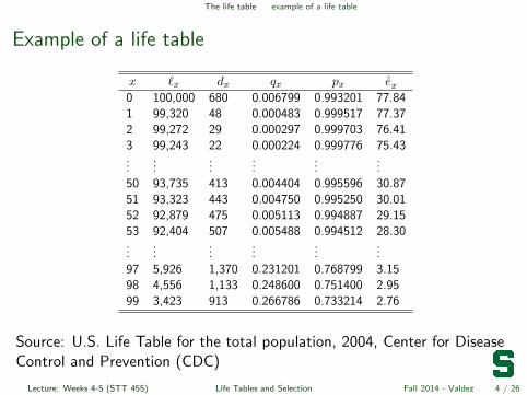
The life table example of a life table
Example of a life table
x `x dx qx px e̊x0 100,000 680 0.006799 0.993201 77.841 99,320 48 0.000483 0.999517 77.372 99,272 29 0.000297 0.999703 76.413 99,243 22 0.000224 0.999776 75.43...
......
......
...50 93,735 413 0.004404 0.995596 30.8751 93,323 443 0.004750 0.995250 30.0152 92,879 475 0.005113 0.994887 29.1553 92,404 507 0.005488 0.994512 28.30...
......
......
...97 5,926 1,370 0.231201 0.768799 3.1598 4,556 1,133 0.248600 0.751400 2.9599 3,423 913 0.266786 0.733214 2.76
Source: U.S. Life Table for the total population, 2004, Center for DiseaseControl and Prevention (CDC)
Lecture: Weeks 4-5 (STT 455) Life Tables and Selection Fall 2014 - Valdez 4 / 26

The life table
Radix of the life table
The radix of the life table does not have to start at age 0, e.g. startwith age x0, so that the table starts with radix `x0 .
The limiting age of the table is usually denoted by ω, in which casethe table ends at ω − x0.
All the formulas still work, e.g. conditional on survival to age x, theprobability of surviving to reach age x+ n is:
pn x = 1− qn x =`x+n`x
.
Note that among `x independent lives who have reached age x, thenumber of survivors Ln within n years is a Binomial random variablewith parameters `x and pn x so that
E(Ln) = `x · pn x.
Lecture: Weeks 4-5 (STT 455) Life Tables and Selection Fall 2014 - Valdez 5 / 26

The life table Table 3.1
Revised example 3.1
Using Table 3.1, page 43 of DHW, calculate the following:
the probability that (30) will survive another 5 years
the probability that (39) will survive to reach age 40
the probability that (30) will die within 10 years
the probability that (30) dies between ages 36 and 38
Lecture: Weeks 4-5 (STT 455) Life Tables and Selection Fall 2014 - Valdez 6 / 26

The life table examples
Illustrative example 1
Complete the following life table:
x `x dx px qx40 24,983 · · ·41 24,541 · · ·42 24,175 · · ·43 23,880 · · ·44 23,656 · · ·45 23,495 − − −
Lecture: Weeks 4-5 (STT 455) Life Tables and Selection Fall 2014 - Valdez 7 / 26

The life table additional useful formulas
Additional useful formulas
From a life table, the following formulas can also easily be verified (or useyour intuition):
`x =∑∞
k=0 dx+k: the number of survivors at age x should be equal tothe number of deaths in each year of age for all the following years.
dn x = `x − `x+n =∑n−1
k=0 dx+k: the number of deaths within n yearsshould be equal to the number of deaths in each year of age for thenext n years.
Finally, the probability that (x) survives the next n years but dies thefollowing m years after that can be derived using:
qn|m x = pn x − pn+m x =dm x+n
`x=`x+n − `x+n+m
`x.
Lecture: Weeks 4-5 (STT 455) Life Tables and Selection Fall 2014 - Valdez 8 / 26

The life table force of mortality
The force of mortality
It is easy to show that the force of mortality can be expressed interms of life table function as:
µx = − 1
`x· d`xdx
.
Thus, in effect, we can also write
`x = `0 · exp
(−∫ x
0µzdz
).
With a simple change of variable, it is easy to see also that
µx+t = − 1
`x+t· d`x+t
dt= − 1
pt x
· d pt x
dt.
It follows immediately that:
d
dtpt x = − pt xµx+t.
Lecture: Weeks 4-5 (STT 455) Life Tables and Selection Fall 2014 - Valdez 9 / 26

The life table curtate expectation of life
Curtate expectation of life
Analogously, the expected value of Kx, is called the curtateexpectation of life defined by
E[Kx] = ex =
∞∑k=0
k pk xqx+k.
It can be shown (e.g. summation by parts) that
ex =
∞∑k=1
pk x =
∞∑k=1
`x+k`x
.
The temporary curtate expectation of life defined by
ex :n =
n∑k=1
pk x =
n∑k=1
`x+k`x
,
which gives the average number of completed years lived over theinterval (x, x+ n] for a life (x).
Lecture: Weeks 4-5 (STT 455) Life Tables and Selection Fall 2014 - Valdez 10 / 26

The life table examples
Illustrative example 2
Suppose you are given the following extract from a life table:
x `x94 16,20895 10,90296 7,21297 4,63798 2,89399 1,747
100 0
1 Calculate e95.
2 Calculate the variance of K95, the curtate future lifetime of (95).
3 Calculate e95: 3
.
Lecture: Weeks 4-5 (STT 455) Life Tables and Selection Fall 2014 - Valdez 11 / 26

The life table typical human mortality curves
age
mo
rta
lity r
ate
s
0
10
20
30
40
50
60
70
80
90
10
0
11
0
12
0
0.0
00
10
.00
10
.01
0.1
1
02
04
06
08
0age
life
exp
ecta
ncy
0
10
20
30
40
50
60
70
80
90
10
0
11
0
12
0
Figure : Source: Life Tables, 2007 from the Social Security Administration - male(blue), female (red)
Lecture: Weeks 4-5 (STT 455) Life Tables and Selection Fall 2014 - Valdez 12 / 26

Fractional age assumptions
Fractional age assumptions
When adopting a life table (which may contain only integer ages),some assumptions are needed about the distribution between theintegers.
The two most common assumptions (or interpolations) used are(where 0 ≤ t ≤ 1):
1 linear interpolation (also called UDD assumption):
`x+t = (1− t)`x + t`x+1
2 exponential interpolation (equivalent to constant force assumption):
log `x+t = (1− t) log `x + t log `x+1
Lecture: Weeks 4-5 (STT 455) Life Tables and Selection Fall 2014 - Valdez 13 / 26

Fractional age assumptions summary of results
Some results on the fractional age assumptions
Linear ExponentialFunction (UDD) (constant force)
qt x t · qx 1− (1− qx)t
µx+tqx
1− t · qxµ = − log px
pt xµx+t qx µe−µt
Here we have 0 ≤ t ≤ 1.
Lecture: Weeks 4-5 (STT 455) Life Tables and Selection Fall 2014 - Valdez 14 / 26

Fractional age assumptions examples
Illustrative example 3
You are given the following extract from a life table:
x `x55 85,91656 84,77257 83,50758 82,114
Estimate p1.4 55 and q0.5|1.6 55 under each of the following assumptions fornon-integral ages:
(a) UDD; and
(b) constant force.
Interpret these probabilities.
Lecture: Weeks 4-5 (STT 455) Life Tables and Selection Fall 2014 - Valdez 15 / 26

Fractional age assumptions
Fractional part of the year lived
Denote by Rx the fractional part of a year lived in the year of death.Then we have
Tx = Kx +Rx
where Tx is the time-until-death and Kx is the curtate future lifetimeof (x).
We can describe the joint probability distribution of (Kx, Rx) as
Pr [(Kx = k) ∩ (Rx ≤ s)] = Pr[k < Tx ≤ k + s] = pk x · qs x+k ,
for k = 0, 1, . . . and for 0 < s < 1.
The UDD assumption is equivalent to the assumption that thefractional part Rx occurs uniformly during the year, i.e. Rx ∼ U(0, 1).
It can be demonstrated that Kx and Rx are independent in this case.
Lecture: Weeks 4-5 (STT 455) Life Tables and Selection Fall 2014 - Valdez 16 / 26

Select and ultimate tables
Select and ultimate tables
Group of lives underwritten for insurance coverage usually hasdifferent mortality than the general population (some test requiredbefore insurance is offered).
Mortality then becomes a function of age [x] at selection (e.g. policyissue, onset of disability) and duration t since selection.
For select tables, notation such as tq[x] , tp[x], and `[x]+t, are thenused.
However, impact of selection diminishes after some time - the selectperiod (denoted by r).
In effect, we haveq[x]+j = qx+j , for j ≥ r.
Lecture: Weeks 4-5 (STT 455) Life Tables and Selection Fall 2014 - Valdez 17 / 26

Select and ultimate tables example of a select and ultimate table
Example of a select and ultimate table
[x] 1000q[x] 1000q[x]+1 1000qx+2 `[x] `[x]+1 `x+2 x+ 2
30 0.222 0.330 0.422 9,907 9,905 9,901 3231 0.234 0.352 0.459 9,903 9,901 9,897 3332 0.250 0.377 0.500 9,899 9,896 9,893 3433 0.269 0.407 0.545 9,894 9,892 9,888 3534 0.291 0.441 0.596 9,889 9,887 9,882 36
From this table, try to compute probabilities such as:
(a) 2p[30];
(b) 5p[30];
(c) 1|q[31]; and
(d) 3q[31]+1.
Lecture: Weeks 4-5 (STT 455) Life Tables and Selection Fall 2014 - Valdez 18 / 26

Select and ultimate tables examples
Illustrative example 4
A select and ultimate table with a three-year select period begins atselection age x.
You are given the following information:
`x+6 = 90, 000
q[x] = 16
p5 [x+1] = 45
p3 [x]+1 = 910 · p3 [x+1].
Evaluate `[x].
Lecture: Weeks 4-5 (STT 455) Life Tables and Selection Fall 2014 - Valdez 19 / 26
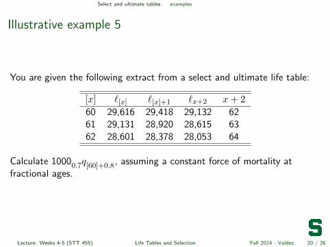
Select and ultimate tables examples
Illustrative example 5
You are given the following extract from a select and ultimate life table:
[x] `[x] `[x]+1 `x+2 x+ 2
60 29,616 29,418 29,132 6261 29,131 28,920 28,615 6362 28,601 28,378 28,053 64
Calculate 1000 q0.7 [60]+0.8, assuming a constant force of mortality atfractional ages.
Lecture: Weeks 4-5 (STT 455) Life Tables and Selection Fall 2014 - Valdez 20 / 26
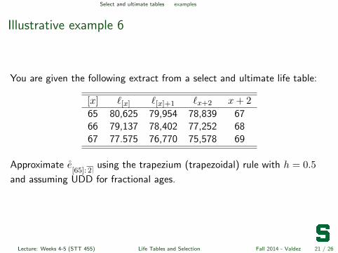
Select and ultimate tables examples
Illustrative example 6
You are given the following extract from a select and ultimate life table:
[x] `[x] `[x]+1 `x+2 x+ 2
65 80,625 79,954 78,839 6766 79,137 78,402 77,252 6867 77.575 76,770 75,578 69
Approximate e̊[65]: 2
using the trapezium (trapezoidal) rule with h = 0.5
and assuming UDD for fractional ages.
Lecture: Weeks 4-5 (STT 455) Life Tables and Selection Fall 2014 - Valdez 21 / 26

Select and ultimate tables examples
Illustrative example 7
The mortality pattern of a life (x) is based on a select and ultimate survivalmodel where the ultimate part follows De Moivre’s law with ω = 80.
You are given:
q[x]+t =
{t+1t+2qx+t, t = 0, 1, 2
qx+t, t = 3, 4, . . .
Calculate the probability that an individual, insured (or selected) one yearago at age 35, will die between age 38 and 40.
Lecture: Weeks 4-5 (STT 455) Life Tables and Selection Fall 2014 - Valdez 22 / 26

Select and ultimate tables examples
Illustrative example 8 - modified SOA MLC Spring 2012
Suppose you are given:
p50 = 0.98
p51 = 0.96
e51.5 = 22.4
The force of mortality is constant between ages 50 and 51.
Deaths are uniformly distributed between ages 51 and 52.
Calculate e50.5.
Lecture: Weeks 4-5 (STT 455) Life Tables and Selection Fall 2014 - Valdez 23 / 26

Select and ultimate tables examples
Illustrative example 9 - modified SOA MLC Spring 2012
In a 2-year select and ultimate mortality table, you are given:
q[x]+1 = 0.96 qx+1
`65 = 82, 358
`66 = 81, 284
Calculate `[64]+1.
Lecture: Weeks 4-5 (STT 455) Life Tables and Selection Fall 2014 - Valdez 24 / 26

Mortality trends
Mortality projection factors
Read Section 3.11
Lecture: Weeks 4-5 (STT 455) Life Tables and Selection Fall 2014 - Valdez 25 / 26

Mortality trends other notation
Only other symbol used in the MLC exam
Expression SOA will adopt
number of lives lx
Lecture: Weeks 4-5 (STT 455) Life Tables and Selection Fall 2014 - Valdez 26 / 26