Lifecycle Portfolio Choice with Tontines

Jan-Hendrik Weinert∗1, Ralph Rogalla2, and Irina Gemmo3

1Department of Finance, Goethe University Frankfurt House of Finance, International Center for InsuranceRegulation (ICIR), Theodor-W.-Adorno-Platz 3, 60629 Frankfurt am Main, Germany

2School of Risk Management, Tobin College of Business, St John’s University, 101 Astor Place, New York, NY10003, United States

3Department of Finance, Goethe University Frankfurt House of Finance, International Center for InsuranceRegulation (ICIR), Theodor-W.-Adorno-Platz 3, 60629 Frankfurt am Main, Germany

February 28, 2018Preliminary Extended Draft: Please do not cite or circulate without the author’s permission

Abstract

We derive the optimal life-cycle portfolio choice and consumption pattern for a CRRAgain-loss utility maximizing investor, facing uncertain labor income, risky capital market re-turns, mortality risk and an age varying level of living standard. In addition to stocks, bondsand deferred annuities, the individuals have access to tontines. Tontines are cost-efficientfinancial contracts providing age-increasing, but volatile cash flows, generated through thepooling of mortality without guarantees, which can help to match increasing financing needsat old ages. We find that tontines can generate significant welfare gains in individuals port-folios. We expect the stake in tontines to increase in age and a maximum level of tontineinvestment for moderate levels of total financial wealth for any age. However, higher riskaversion reduces tontine investments. At retirement, deferred annuities account for the ma-jority of total financial wealth, supplemented by a notable level of tontine investment.

Keywords: Tontines, Life Insurance, Consumption, Annuities, Mortality, Retirement Plan-ning, Consumption-portfolio choice, Deferred life annuitiesJEL Classification: D14, E21, G22, I31, J10, L51

∗Corresponding author

1 Introduction

Demographic change and the associated shift in the age structure of the population make it

increasingly difficult to secure the funding of pay-as-you-go pension systems in many Western

societies. Declining birth rates and simultaneously increasing life expectancy worldwide1 lead to

an increase in benefit recipients of the statutory pension insurance with a simultaneous decrease

in contributors. The associated increase in the so-called pension ratio makes it more difficult

to maintain pay-as-you-go pension systems, such as the public pension system in Germany. In

return, funded pension products and private pensions are gaining in importance. This challenge

of an aging society is intensified by increasing funding needs in old age2.

The medical advances of the past decades cause that a multitude of diseases and ailments can

now be cured, that would have lead to death 50 years ago3. However, these medical measures

and treatment methods are often associated with enormous costs and increase especially in

old age, when afflictions pile up. Thus, e.g. a costly, elderly-friendly conversion or expansion

of the home will be necessary, which allows the longest possible and independent living in

the familiar environment. Furthermore, very high costs for ambulatory and inpatient care are

incurred in old age. However, specialized health insurance often depends on the level of care and

includes derogations so that soft factors and uninsured aspects are not covered. These include,

for example, costly items to maintain the standard of living (e.g., dependence on taxi services

because of visual impairment or the use of high quality meal-on-wheels services or shopping

delivery services), or the delivery of high-quality nutritional services beyond the statutory level

(e.g., massages or home help).

This raises the need for a pension product that is suitable to meet the rising capital requirements

at retirement age at low cost. These considerations lead to the principle of tontines, which has

been adapted to current conditions to meet the requirements of the 21st century.

1 According to the Worldbank (2015), worldwide life expectancy at birth has increased between 1960 and 2015from 52.5 to above 71.7 years. The increasing lifetime will cause the number of people over 80 years old toalmost double to 9 million in Germany by the year 2060 according to forecasts by the Statistisches Bundesamt(2015). In the future, it is therefore very probable that very high ages of 100 years and even more will beachieved by a large number of people.

2 According to the medicalisation thesis motivated by Gruenberg (1977), the additional years that peoplelive due to demographic change are increasingly spent in bad health condition and disability. Jagger et al.(2016) find a significant increase in life expectancy between 1991 and 2011 in England. In those additionalyears of life, the demand for care products and medical service increases over-proportionately. Coming from2.6 million nursing cases in Germany in 2013, Kochskamper (2015) estimates between 1.5 and 1.9 millionadditional nursing cases in Germany in the year 2060 due to demographic change. By the year 2030, thedemand for stationary permanent care will increase by 220,000 places in Germany. A study by Standard Life(2013) shows that an 85-year-old person on average has six times higher total spending than a comparable65-year-old person.

3 For example, the invention of penicillin and other antibiotics in the 1940s and 1950s or the ability of medicaltreatment of cardiovascular diseases in the 1960s lowered the mortality rates for all age groups.

1

The tontine is a financial product developed by its eponymous inventor, Lorenzo de Tonti, in the

1650s for long-term public funding of the French state. In their original form, each tontine owner

received a lifelong annual pension in exchange for a one-off payment to the French State. The

shares of deceased tontine members are spread among the survivors, increasing their pension

payments. Payments to surviving tontinists therefore increase over time. According to this

mechanism, the last survivor receives the pension payments from everyone else.

A tontine thus offers an age-increasing payout structure without the need of guarantees, which

is generated by the diversification of mortality between policyholders. This peculiarity makes

tontines appear extremely interesting against the backdrop of an increasing need for capital in

old age, since a small amount of funds can generate very high payouts in old age.

As a result of these developments, tontines are becoming increasingly important. McKeever

(2009), Milevsky (2015) and Li and Rothschild (2017) work up the historical development of

tontines, Sabin (2010), Milevsky and Salisbury (2015) and Milevsky and Salisbury (2016) focus

on the actuarial fair and optimal payout structure of a tontine and Chen et al. (2017) combine a

tontine and an annuity into a common product. In Weinert (2017b) the tontine is supplemented

with a cancellation option and its effects on the other tontinists is determined as well as the fair

cancellation amount. Weinert (2017a) estimates the cost of a tontine compared to traditional

life insurance products from an economic as well as an regulatory perspective. In Weinert and

Grundl (2016), tontines are studied for suitability as a complement to traditional retirement

products, taking into account the aforementioned demographic challenges. The authors analyze

whether a tontine is suitable for serving the increasing financial needs of elderly people. However,

that article aims to find the fundamental effects of tontinization and therefore, the model assumes

that individuals care about gains and losses in wealth in a simplified framework without capital

markets. To analyze this topic with a holistic approach, we include the tontine in a standard

life-cycle framework4 and identify the optimal portfolio structure considering gains and losses

in consumption. Due to the over proportional increase in cost with age to maintain a constant

level of living standard, we incorporate an age increasing external habit into the model and

derive the optimal consumption, saving and portfolio choice pattern for a CRRA gain-loss utility

maximizing investor, facing uncertain labor income and risky capital market returns. First

results indicate that it is optimal for medium wealthy individuals to increase the stake in tontine

investments with age to maximize expected lifetime utility.

In Section 2, we introduce the life-cycle model applied to find the optimal consumption and

4 See for example Horneff et al. (2010), Hubener et al. (2013), Maurer et al. (2013) and Horneff et al. (2015).

2

portfolio allocation into stocks, bonds, deferred annuities and tontines. We solve the model

numerically and present the our expected results in Section 3. We discuss the optimal life-cycle

asset allocation for the base case. Further, we vary the calibrations of key parameters and

determine the expected life-cycle profiles.

2 The Model

We assume that an individual has no bequest motive and has access to capital markets by

investing in risk-free bonds, risky stocks, risky tontines and deferred life annuities.

Utility:

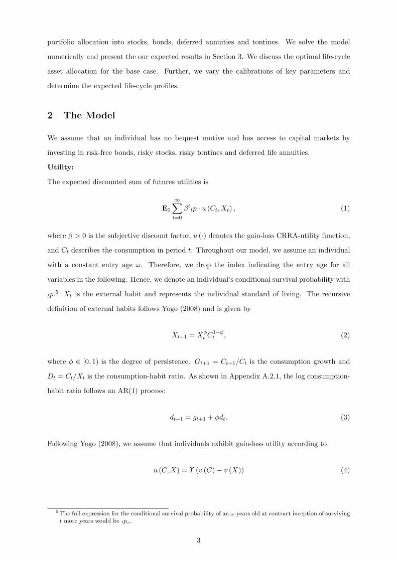
The expected discounted sum of futures utilities is

E0

∞∑t=0

βttp · u (Ct, Xt) , (1)

where β > 0 is the subjective discount factor, u (·) denotes the gain-loss CRRA-utility function,

and Ct describes the consumption in period t. Throughout our model, we assume an individual

with a constant entry age ω. Therefore, we drop the index indicating the entry age for all

variables in the following. Hence, we denote an individual’s conditional survival probability with

tp.5 Xt is the external habit and represents the individual standard of living. The recursive

definition of external habits follows Yogo (2008) and is given by

Xt+1 = Xφt C

1−φt , (2)

where φ ∈ [0, 1) is the degree of persistence. Gt+1 = Ct+1/Ct is the consumption growth and

Dt = Ct/Xt is the consumption-habit ratio. As shown in Appendix A.2.1, the log consumption-

habit ratio follows an AR(1) process:

dt+1 = gt+1 + φdt. (3)

Following Yogo (2008), we assume that individuals exhibit gain-loss utility according to

u (C,X) = Υ (v (C)− v (X)) (4)

5 The full expression for the conditional survival probability of an ω years old at contract inception of survivingt more years would be tpω.

3

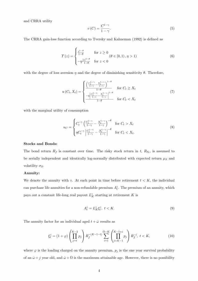
and CRRA utility

v (C) =C1−γ

1− γ. (5)

The CRRA gain-loss function according to Tversky and Kahneman (1992) is defined as

Υ (z) =

z1−θ

1−θ for z ≥ 0

−η |z|1−θ

1−θ for z < 0

(θ ∈ [0, 1) , η > 1) (6)

with the degree of loss aversion η and the degree of diminishing sensitivity θ. Therefore,

u (Ct, Xt) =

(C1−γt1−γ

−X1−γt1−γ

)1−θ

1−θ for Ct ≥ Xt

−η∣∣∣∣C1−γ

t1−γ

−X1−γt1−γ

∣∣∣∣1−θ

1−θ for Ct < Xt

(7)

with the marginal utility of consumption

uC =

C−γt

(C1−γ

t1−γ − X1−γ

t1−γ

)−θfor Ct > Xt

ηC−γt

∣∣∣C1−γt1−γ − X1−γ

t1−γ

∣∣∣−θ for Ct < Xt.

(8)

Stocks and Bonds:

The bond return Rf is constant over time. The risky stock return in t, RSt , is assumed to

be serially independent and identically log-normally distributed with expected return µS and

volatility σS .

Annuity:

We denote the annuity with . At each point in time before retirement t < K, the individual

can purchase life annuities for a non-refundable premium At . The premium of an annuity, which

pays out a constant life-long real payout LK starting at retirement K is

At = L

Kξt , t < K. (9)

The annuity factor for an individual aged t+ ω results as

ξt = (1 + ϕ)

K−2∏j=t

pj

R−(K−1−t)f

Ω−K∑i=1

K−1+i∏j=K−1

pj

R−if , t < K, (10)

where ϕ is the loading charged on the annuity premium, pj is the one year survival probability

of an ω+ j year old, and ω+Ω is the maximum attainable age. However, there is no possibility

4

to surrender the annuity contracts.

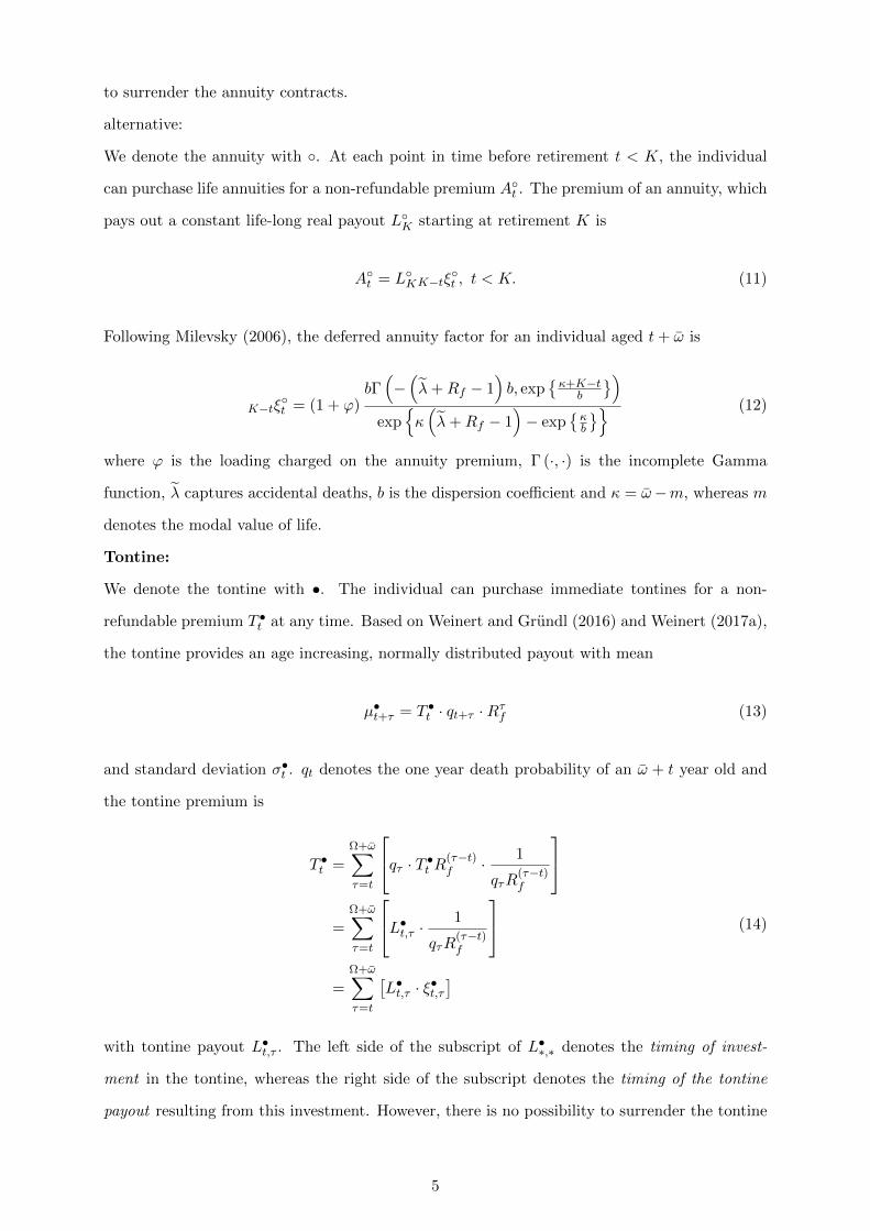
alternative:

We denote the annuity with . At each point in time before retirement t < K, the individual

can purchase life annuities for a non-refundable premium At . The premium of an annuity, which

pays out a constant life-long real payout LK starting at retirement K is

At = L

KK−tξt , t < K. (11)

Following Milevsky (2006), the deferred annuity factor for an individual aged t+ ω is

K−tξt = (1 + ϕ)

bΓ(−(λ+Rf − 1

)b, exp

κ+K−t

b

)exp

κ(λ+Rf − 1

)− exp

κb

(12)

where ϕ is the loading charged on the annuity premium, Γ (·, ·) is the incomplete Gamma

function, λ captures accidental deaths, b is the dispersion coefficient and κ = ω−m, whereas m

denotes the modal value of life.

Tontine:

We denote the tontine with •. The individual can purchase immediate tontines for a non-

refundable premium T •t at any time. Based on Weinert and Grundl (2016) and Weinert (2017a),

the tontine provides an age increasing, normally distributed payout with mean

µ•t+τ = T •

t · qt+τ ·Rτf (13)

and standard deviation σ•t . qt denotes the one year death probability of an ω + t year old and

the tontine premium is

T •t =

Ω+ω∑τ=t

qτ · T •t R

(τ−t)f · 1

qτR(τ−t)f

=

Ω+ω∑τ=t

L•t,τ ·

1

qτR(τ−t)f

=

Ω+ω∑τ=t

[L•t,τ · ξ•t,τ

](14)

with tontine payout L•t,τ . The left side of the subscript of L•

∗,∗ denotes the timing of invest-

ment in the tontine, whereas the right side of the subscript denotes the timing of the tontine

payout resulting from this investment. However, there is no possibility to surrender the tontine

5

contracts.

LTC insurance:

In an alternative scenario, we assume that the individual has the opportunity to invest in

long-term-care (LTC) contracts, which cover some of the old age expenses. The pricing of the

LTC contract follows Levikson and Mizrahi (1994).

Labor Income:

Labor income (t < K) is determined as

Yt =

exp h (t)PtΨt for t < K

ζ exp h (t)Pt for t ≥ K.

(15)

where the permanent component Pt depends on its value in the previous period and innovation

Nt:

Pt = Pt−1Nt. (16)

The function h (t) describes the empirically calibrated hump shaped income profile during work

life and Ψt displays a transitory shock. ln (Nt) and ln (Ψt) are normally distributed with mean

zero and standard deviation σn and σψ. During retirement (t ≥ K), the individual receives a

constant pension, where ζ is the constant replacement rate.

Wealth accumulation:

The available wealth Wt can be invested in bonds Bt, stocks St, annuities At (if not retired,

t < K), tontines T •t and consumption Ct. The budget constraint is:

Wt =

Bt + St +A

t + T •t + Ct for t < K

Bt + St + T •t + Ct for t ≥ K.

(17)

Bt + St compounds to the financial wealth. Individual disposable wealth in t+ 1 is

Wt+1

BtRf + StRSt+1 +

∑tτ=0 L

•τ,t+1 + Yt+1 for t < K

BtRf + StRSt+1 +∑t

τ=0 L•τ,t+1 + L

t+1 + Yt+1 for t ≥ K.

(18)

BtRf + StRt+1 describes the value of financial wealth in t + 1 and Yt+1 is the labor income

(before retirement) or retirement income (from retirement on).∑t

τ=0 L•τ,t+1 is the sum of the

tontine income of all periods invested in the tontine, whereas Lt+1 is the sum of annuity income

of all periods invested in the annuity:

6

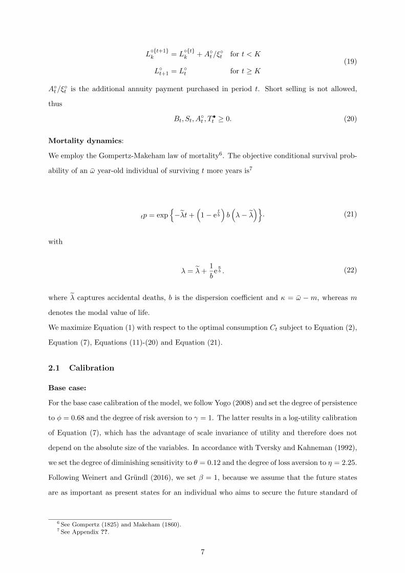
Lt+1k = L

tk +A

t /ξt for t < K

Lt+1 = L

t for t ≥ K

(19)

At /ξ

t is the additional annuity payment purchased in period t. Short selling is not allowed,

thus

Bt, St, At , T

•t ≥ 0. (20)

Mortality dynamics:

We employ the Gompertz-Makeham law of mortality6. The objective conditional survival prob-

ability of an ω year-old individual of surviving t more years is7

tp = exp−λt+

(1− e

tb

)b(λ− λ

). (21)

with

λ = λ+1

be

κb . (22)

where λ captures accidental deaths, b is the dispersion coefficient and κ = ω − m, whereas m

denotes the modal value of life.

We maximize Equation (1) with respect to the optimal consumption Ct subject to Equation (2),

Equation (7), Equations (11)-(20) and Equation (21).

2.1 Calibration

Base case:

For the base case calibration of the model, we follow Yogo (2008) and set the degree of persistence

to φ = 0.68 and the degree of risk aversion to γ = 1. The latter results in a log-utility calibration

of Equation (7), which has the advantage of scale invariance of utility and therefore does not

depend on the absolute size of the variables. In accordance with Tversky and Kahneman (1992),

we set the degree of diminishing sensitivity to θ = 0.12 and the degree of loss aversion to η = 2.25.

Following Weinert and Grundl (2016), we set β = 1, because we assume that the future states

are as important as present states for an individual who aims to secure the future standard of

6 See Gompertz (1825) and Makeham (1860).7 See Appendix ??.

7

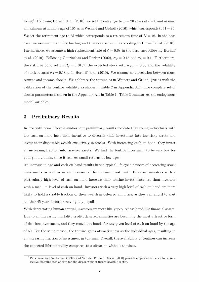
living8. Following Horneff et al. (2010), we set the entry age to ω = 20 years at t = 0 and assume

a maximum attainable age of 105 as in Weinert and Grundl (2016), which corresponds to Ω = 86.

We set the retirement age to 65 which corresponds to a retirement time of K = 46. In the base

case, we assume no annuity loading and therefore set ϕ = 0 according to Horneff et al. (2010).

Furthermore, we assume a high replacement rate of ζ = 0.68 in the base case following Horneff

et al. (2010). Following Gourinchas and Parker (2002), σψ = 0.15 and σn = 0.1. Furthermore,

the risk free bond return Rf = 1.0137, the expected stock return µS = 0.06 and the volatility

of stock returns σS = 0.18 as in Horneff et al. (2010). We assume no correlation between stock

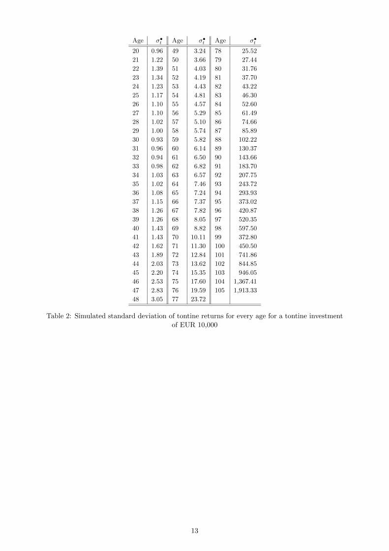
returns and income shocks. We calibrate the tontine as in Weinert and Grundl (2016) with the

calibration of the tontine volatility as shown in Table 2 in Appendix A.1. The complete set of

chosen parameters is shown in the Appendix A.1 in Table 1. Table 3 summarizes the endogenous

model variables.

3 Preliminary Results

In line with prior lifecycle studies, our preliminary results indicate that young individuals with

low cash on hand have little incentive to diversify their investment into less-risky assets and

invest their disposable wealth exclusively in stocks. With increasing cash on hand, they invest

an increasing fraction into risk-free assets. We find the tontine investment to be very low for

young individuals, since it realizes small returns at low ages.

An increase in age and cash on hand results in the typical life-cycle pattern of decreasing stock

investments as well as in an increase of the tontine investment. However, investors with a

particularly high level of cash on hand increase their tontine investments less than investors

with a medium level of cash on hand. Investors with a very high level of cash on hand are more

likely to hold a sizable fraction of their wealth in deferred annuities, as they can afford to wait

another 45 years before receiving any payoffs.

With depreciating human capital, investors are more likely to purchase bond-like financial assets.

Due to an increasing mortality credit, deferred annuities are becoming the most attractive form

of risk-free investment, and they crowd out bonds for any given level of cash on hand by the age

of 60. For the same reason, the tontine gains attractiveness as the individual ages, resulting in

an increasing fraction of investment in tontines. Overall, the availability of tontines can increase

the expected lifetime utility compared to a situation without tontines.

8 Parsonage and Neuburger (1992) and Van der Pol and Cairns (2000) provide empirical evidence for a sub-jective discount rate of zero for the discounting of future health benefits.

8

References

Chen, A., Hieber, P., and Klein, J. (2017). Tonuity: A novel individual-oriented retirement plan.

Working paper, available at SSRN 3043013.

Cocco, J. F., Gomes, F. J., and Maenhout, P. J. (2005). Consumption and portfolio choice over

the life cycle. The Review of Financial Studies, 18(2):491–533.

Gompertz, B. (1825). On the nature of the function expressive of the law of human mortality,

and on a new mode of determining the value of life contingencies. Philosophical Transactions of

the Royal Society of London, 115:513–583.

Gourinchas, P.-O. and Parker, J. A. (2002). Consumption over the life cycle. Econometrica,

70(1):47–89.

Gruenberg, E. M. (1977). The failures of success. The Milbank Memorial Fund Quarterly. Health

and Society, 55(1):3–24.

Horneff, V., Maurer, R., Mitchell, O. S., and Rogalla, R. (2015). Optimal life cycle portfolio

choice with variable annuities offering liquidity and investment downside protection. Insurance:

Mathematics and Economics, 63:91–107.

Horneff, W., Maurer, R., and Rogalla, R. (2010). Dynamic portfolio choice with deferred annu-

ities. Journal of Banking & Finance, 34(11):2652–2664.

Hubener, A., Maurer, R., and Rogalla, R. (2013). Optimal portfolio choice with annuities and

life insurance for retired couples. Review of Finance, 18(1):147–188.

Jagger, C., Matthews, F. E., Wohland, P., Fouweather, T., Stephan, B. C., Robinson, L., Arthur,

A., Brayne, C., Function, M. R. C. C., Collaboration, A., et al. (2016). A comparison of health

expectancies over two decades in England: results of the cognitive function and ageing study i

and ii. The Lancet, 387(10020):779–786.

Kochskamper, Susanna und Pimpertz, J. (2015). Herausforderungen an diePflegeinfrastruktur.

IW-Trends Vierteljahresschrift zur empirischen Wirtschaftsforschung, 42(3).

Levikson, B. and Mizrahi, G. (1994). Pricing long term care insurance contracts. Insurance:

Mathematics and Economics, 14(1):1–18.

Li, Y. and Rothschild, C. (2017). Adverse selection and redistribution in the irish tontines of

1773, 1775 and 1777. Working Paper.

9

Makeham, W. M. (1860). On the law of mortality and the construction of annuity tables. The

Assurance Magazine, and Journal of the Institute of Actuaries, 8(6):301–310.

Maurer, R., Mitchell, O. S., and Rogalla, R. (2010). The effect of uncertain labor income and

social security on life-cycle portfolios. Technical report, National Bureau of Economic Research.

Maurer, R., Mitchell, O. S., Rogalla, R., and Kartashov, V. (2013). Lifecycle portfolio choice

with systematic longevity risk and variable investmentlinked deferred annuities. Journal of Risk

and Insurance, 80(3):649–676.

McKeever, K. (2009). Short history of tontines, a. Fordham J. Corp. & Fin. L., 15:491.

Milevsky, M. A. (2006). The calculus of retirement income: Financial models for pension annu-

ities and life insurance. Cambridge University Press.

Milevsky, M. A. (2015). King William’s tontine: why the retirement annuity of the future should

resemble its past. Cambridge University Press.

Milevsky, M. A. and Salisbury, T. S. (2015). Optimal retirement income tontines. Insurance:

Mathematics and Economics, 64:91–105.

Milevsky, M. A. and Salisbury, T. S. (2016). Equitable retirement income tontines: Mixing

cohorts without discriminating. ASTIN Bulletin: The Journal of the IAA, 46(3):571–604.

Parsonage, M. and Neuburger, H. (1992). Discounting and health benefits. Health economics,

1(1):71–76.

Sabin, M. J. (2010). Fair tontine annuity. Social Science Research Network Working Paper

Series.

Standard Life (2013). The retirement smile. http://ukgroup.standardlife.com/content/

news/new_articles/2013/260613NewDrawdownTransferOption.xml.

Statistisches Bundesamt (2015). Bevolkerung Deutschlands bis 2060: 13.

koordinierte Bevolkerungsvorausberechnung. https://www.destatis.de/DE/

Publikationen/Thematisch/Bevoelkerung/VorausberechnungBevoelkerung/

BevoelkerungDeutschland2060Presse5124204159004.pdf?__blob=publicationFile.

Tversky, A. and Kahneman, D. (1992). Advances in prospect theory: Cumulative representation

of uncertainty. Journal of Risk and uncertainty, 5(4):297–323.

10

Van der Pol, M. M. and Cairns, J. A. (2000). Negative and zero time preference for health.

Health Economics, 9(2):171–175.

Weinert, J.-H. (2017a). Comparing the cost of a tontine with a tontine replicating annuity. ICIR

Working Paper Series, (31/2017).

Weinert, J.-H. (2017b). The fair surrender value of a tontine. ICIR Working Paper Series,

(26/2017).

Weinert, J.-H. and Grundl, H. (2016). The modern tontine: An innovative instrument for

longevity risk management in an aging society. ICIR Working Paper Series, (22/2016).

Worldbank (2015). Databank. Life expectancy at birth. http://data.worldbank.org/

indicator/SP.DYN.LE00.IN.

Yogo, M. (2008). Asset prices under habit formation and reference-dependent preferences. Jour-

nal of Business & Economic Statistics, 26(2):131–143.

11

A Appendix

A.1 Tables

Variable Description Value Sourceβ Subjective discount factor 1 Parsonage and Neuburger (1992)

Van der Pol and Cairns (2000)Weinert and Grundl (2016)

t Time 0...86 Horneff et al. (2010)ω Entry age 20 Horneff et al. (2010)φ Degree of persistence 0.68 Yogo (2008)θ Degree of diminishing sensitivity 0.12 Tversky and Kahneman (1992)η Degree of loss aversion 2.25 Tversky and Kahneman (1992)γ Degree of risk aversion 1 Yogo (2008)Rf Risk free bond return 1.0137 Yogo (2008)µS Expected stock return 1.06 Horneff et al. (2010)σS Volatility of stock return 0.18 Horneff et al. (2010)K Retirement time 46 Horneff et al. (2010)ϕ Loading charged on annuity premium 0 Maurer et al. (2010)

Horneff et al. (2010)Ω Maximum time of an individual in the

model86 Weinert and Grundl (2016)

σ•t Standard deviation of tontine returns in t Table 2 Weinert and Grundl (2016)

h (·) Income shape profile Cocco et al. (2005)Horneff et al. (2010)

Pt Permanent component of income in t Cocco et al. (2005)Horneff et al. (2010)

Ψt Transitory shock in t Horneff et al. (2010)Nt Innovation in t Horneff et al. (2010)σn Standard deviation of ln (Nt) in t 0.1 Gourinchas and Parker (2002)

Horneff et al. (2010)σψ Standard deviation of ln (Ψt) in t 0.15 Gourinchas and Parker (2002)

Horneff et al. (2010)ζ Constant replacement rate 0.68 Cocco et al. (2005)

Horneff et al. (2010)λ Accidental death 0 Milevsky (2006)b Dispersion coefficient 11.4 Milevsky (2006)m Modal value of life 82.3 Milevsky (2006)

Table 1: Calibration base case

12

Age σ•t Age σ•

t Age σ•t

20 0.96 49 3.24 78 25.52

21 1.22 50 3.66 79 27.44

22 1.39 51 4.03 80 31.76

23 1.34 52 4.19 81 37.70

24 1.23 53 4.43 82 43.22

25 1.17 54 4.81 83 46.30

26 1.10 55 4.57 84 52.60

27 1.10 56 5.29 85 61.49

28 1.02 57 5.10 86 74.66

29 1.00 58 5.74 87 85.89

30 0.93 59 5.82 88 102.22

31 0.96 60 6.14 89 130.37

32 0.94 61 6.50 90 143.66

33 0.98 62 6.82 91 183.70

34 1.03 63 6.57 92 207.75

35 1.02 64 7.46 93 243.72

36 1.08 65 7.24 94 293.93

37 1.15 66 7.37 95 373.02

38 1.26 67 7.82 96 420.87

39 1.26 68 8.05 97 520.35

40 1.43 69 8.82 98 597.50

41 1.43 70 10.11 99 372.80

42 1.62 71 11.30 100 450.50

43 1.89 72 12.84 101 741.86

44 2.03 73 13.62 102 844.85

45 2.20 74 15.35 103 946.05

46 2.53 75 17.60 104 1,367.41

47 2.83 76 19.59 105 1,913.33

48 3.05 77 23.72

Table 2: Simulated standard deviation of tontine returns for every age for a tontine investmentof EUR 10,000

13

Variable Description

tp Conditional survival probability

Ct Consumption in t

Xt External habit in t

u (·) Utility

Gt+1 Consumption growth

Dt Consumption habit ratio

Υ (·) Gain-loss function

v (·) CRRA-utility

uC Marginal utility of consumption

RStRisky stock return in t

At Annuity premium in t

T •t Tontine premium t

LK Constant real annuity payout beginning from K

ξt Annuity factor for individual aged ω + t

pt One year survival probability of an ω + t year old individual

µ•t Tontine payout mean in t

qt One year death probability of an ω + t year old individual

L•t,τ Tontine payout in τ for tontine premium paid in t

ξ•t,τ Tontine discount factor in τ for premium paid in t

Yt Labor/retirement income in t

Wt Available wealth

Bt Bond investment

St Stock investment

λt Objective hazard function of an ω year old of dying at the age of ω + t

F (t) Probability of an ω old individual of dying before the age of ω + t

f (t) PDF

Table 3: Endogenous model variables

A.2 Proofs

A.2.1 Log Consumption-Habit Ratio

ln (Dt+1) = ln

(Ct+1

Xt+1

)= ln

(Ct+1

Xφt C

1−φt

)

= ln (Ct+1)− ln(Xφt C

1−φt

)= ln (Ct+1)− ln

(Xφt

)− ln

(C1−φt

)= ln (Ct+1)− φ ln (Xt)− (1− φ) ln (Ct)

= ln (Ct+1)− φ ln (Xt)− ln (Ct) + φ ln (Ct)

= ln

(Ct+1

Ct

)+ φ ln

(CtXt

)ln (Dt+1) = ln (Gt+1) + φ ln (Dt)

dt+1 = gt+1 + φdt

14