Lifted Auto-Context Forests for Brain TumourSegmentation

Loic Le Folgoc, Aditya V. Nori, Siddharth Ancha, and Antonio Criminisi

Microsoft Research Cambridge, UK.

Abstract. We revisit Auto-Context Forests for brain tumour segmentation inmulti-channel magnetic resonance images, where semantic context is progres-sively built and refined via successive layers of Decision Forests (DFs). Specifi-cally, we make the following contributions: 1) improved generalization via an ef-ficient node-splitting criterion based on hold-out estimates, 2) increased compact-ness at a tree-level, thereby yielding shallow discriminative ensembles trainedorders of magnitude faster, and 3) guided semantic bagging that exposes latentdata-space semantics captured by forest pathways. The proposed framework ispractical: the per-layer training is fast, modular and robust. It was a top performerin the MICCAI 2016 BRATS (Brain Tumour Segmentation) challenge, and thispaper aims to discuss and provide details about the challenge entry.

1 Introduction

The past few years have witnessed a vast body of machine learning (ML) techniquesfor the automatic segmentation of medical images. Decision forests (DFs) [21,18], andmore recently, deep neural networks [11] have yielded state-of-the-art results at MIC-CAI BRATS (Brain Tumour Segmentation) challenges.

In this paper, we describe an approach that builds upon the framework of DFs, de-parting from the usual hand-crafting of powerful features based on e.g. texture, elasticregistration, supervoxels [17,6] with a complementary scheme that is entirely genericand free of additional computations. More specifically, we introduce an efficient node-splitting criterion based on cross-validation estimates that improves the feature selec-tion during the training stage. Consequently, learnt features are more discriminative andgeneralize better to unseen data: we refer to this process as lifting (see Section 4). Fur-thermore, the proposed cost function induces a natural stopping condition to grow orprune decision trees, resulting in an Occam’s razor-like, principled trade-off betweentree complexity and training accuracy. We show that lifted DFs can outperform standardDFs using compact, shallow tree architectures (several dozens or hundreds of nodes).

We exploit the resulting computational gains to revisit auto-context [14,15,13] seg-mentation forests. In particular, we extend the approach with a meta-architecture of cas-caded DFs that naturally intertwine high-level semantic reasoning with intensity-basedlow-level reasoning (described in Section 5). The framework aims to be practical: theper-layer training is simple, modular and robust. Furthermore, this sequential design en-ables the decomposition of complex segmentation tasks into series of simpler subtasksthat, for instance, exploit the hierarchical structure between labels (e.g., whole tumour,

2 Le Folgoc et al.

tumour core, enhancing tumour parts). Beyond auto-context, another contribution is aclustering mechanism (see Section 5.2) that exposes the latent data-space semantics en-coded within DF pathways. The learnt semantics are exploited to automatically guideclassification in subsequent layers. Finally, in Section 7, we discuss results and detailsof our BRATS challenge entry.

2 Background: Random Forests for Image Segmentation

Let I = {Ij}j=1···J be the set of input channels in a multichannel image, x be a voxel,and c ∈ C = {1 . . .K} be the class to predict for x. We define x = {x, I} ∈ X as thefeature vector of x. DF classifiers predict the probability p(c|x) that a voxel x belongsto class c given its feature representation x. This is done by aggregating predictions ofan ensemble of T decision trees. Simple averaging is typically used, so that:

p(c|x)=1/|T | ·|T |∑t=1

pt(c|x) ,

where pt(c|x) denotes the prediction by tree t ∈ T . The class with maximum probabil-ity is then returned (maximum a posteriori probability) as the prediction. Tree predic-tions are obtained as follows: a feature vector x is routed along a path in the tree fromthe root node by evaluating it at every internal (split) node n w.r.t. a routing functionhn(x) , [f(x,θn)≤ τn] ∈ {0, 1}, and taking the left child nL if hn(x) = 1, and theright child nR otherwise, until a leaf node n(x) is reached. Here f : X ×Θ 7→ Ris a weak learner parameterized by a node-specific feature θn ∈ Θ, and τn ∈ R anode-specific threshold. Examples of weak learners are given in section 3. Each ter-minal (leaf ) node n ∈ L is paired with a class predictor pn(c|x) , pn(c) such that0≤pn(c)≤1,

∑Kc=1 pn(c)=1. The tree then predicts class c with probability pn(x)(c).

Decision trees are trained in a supervised manner from training dataD={xi, ci}Ni=1

with known class labels ci, greedily and recursively, starting from a single root node.Training a node n entails finding the optimal feature θ∗n and threshold τ∗n such that thenode training data Dn={xi, ci}i∈In is split between left and right children nL and nRin a way that maximizes class purity. Specifically, ψ∗=(θ∗n, τ

∗n) and the resulting split

Dn=DnL(ψ)∐DnR(ψ) maximizes the Information Gain G(ψ;Dn), which is defined

as follows:

G(ψ;Dn) ,∑

ε={L,R}

|Dnε(ψ)||Dn|

∑c∈C

pnε(c;ψ) log pnε(c;ψ)−∑c∈C

p∗n(c) log p∗n(c) , (1)

where pnε(c;ψ) , |{i∈Inε(ψ)|ci=c}| / |Dnε(ψ)| is the empirical class distribution inthe training data Dnε for the child node nε. The optimum ψ∗,argmaxψ G(ψ;Dn) isfound by exhaustive search after proper quantization of thresholds τn. Trees are grownup to a predefined maximum depth, or until the number of training examples reachinga node is below a given threshold.

Last but not least, random forests introduce randomization in the training of eachtree via feature and data bagging. For the t-th tree and at node n ∈ Vt, only a random

Lifted Auto-Context Forests for BRATS 3

subset Θ′ Θ of candidate features is considered for training [1,7]. Similarly, only arandom subset D′n Dn of training examples sampled with(out) replacement is used[3]. Data bagging is implemented both at an image level (random image subsets) and ata voxel level (random voxel subsets).

It is important to note that we do not make use of class rebalancing schemes. Train-ing samples are often weighted according to the relative frequency of their class. Thisstrategy aims to correct classifier bias in favor of the more frequent class, in cases wherethere is a large class imbalance. Of course, class rebalancing induces the opposite biasagainst more prevalent classes, which cannot be avoided in a multilabel classificationsetting. Section 5.2 discusses an alternative strategy to naturally correct for distributionimbalance.

3 Fast scale-space context-sensitive features

We revisit scale-space representations to craft fast, expressive, compactly parameter-ized features, as a simple alternative to the popular integral or Haar-like features [19].

Background: integral features. Integral features are based on intensity averages withinanisotropic cuboids offset from the point of interest [5]. Cuboid averages are computedin constant time by probing the value of a precomputed integral map at the cuboid ver-tices [19]. For instance, f(x,θ),

∑x′∈C2Ij2(x

′) −∑x′∈C1Ij1(x

′) computes the dif-ference of responses in cuboids C1 and C2 of size s1=(sx1 , s

y1, s

z1) and s2=(sx2 , s

y2, s

z2),

centered at offset locations x + o1 and x + o2, in distinct channels Ij1 and Ij2 . Hereθ=(j1, j2,o1,o2, s1, s2) is a 14-dimensional feature.

Proposed scale-space representation. During node training, it is crucial for suffi-ciently strong weak-learners to be computable within the budget allocated to featuresampling and optimization. Therefore, reducing the feature parameterization while main-taining expressiveness is key. For integral features, the sophistication of probing anisotropiccuboids with a continuous range of edge lengths comes at a cost w.r.t. parametric com-plexity. We restrict ourselves to a small finite range of isotropic averages. We augmentthe original set of c input channels with their smoothed counterparts under separableGaussian filtering at scales σ1, σ2 etc. Given s scales, f(x,θ),Ij2(x+o2)−Ij1(x+o1)computes the difference of responses in different channels at different scales and off-sets from the voxel of interest (j∈{1 . . . c×s} flatly indexes channels and scales). Hereθ=(j1, j2,o1,o2) is an 8-dimensional feature.

A single point is probed for every 8 cuboid vertices probed under integral features,as well as circumventing many boundary checks. For all practical purposes (s = 2, 3),byte[] storage of scale-space maps limits the memory overhead relative to integralmaps (short[] storage).

Fast rotation invariant features. We can go beyond directional context and account fornatural local invariances with fast, multiscale, approximately rotation invariant feature.Let φ1 · · ·φ12 stand for the coordinates of an axis-aligned, centered icosahedron of ra-dius r. Denoting by θ=(j1, j2, r) the 3-dimensional feature, f(x,θ),Median12v=1|Ij2(x+

4 Le Folgoc et al.

φv)−Ij1(x)| gives a robust summary of intensity variations around point x and probes13 points only.

4 Lifting Decision Forests by Minimizing Cross-Validation ErrorEstimates

4.1 A cautionary look at Information Gain maximizationWe follow the notation introduced in Section 2, but drop the node index n for conve-nience. Information gain maximization w.r.t. (feature, threshold) parameters ψ = (θ, τ)can be shown to be equivalent to a joint maximum likelihood estimation (MLE) ofφ , (ψ, pL, pR), the node parameters and children’ class predictors. We omit the de-tails for the sake of brevity. Essentially, decision trees are usually grown by greedily,recursively splitting leaf nodes by likelihood maximization:

φ∗ = argmaxφ

C(D;φ) , argmaxφ

p(D;φ)

p∗(D). (2)

In Eq. (2), the denominator is the data likelihood using the current leaf node predictor,whereas the numerator is the data likelihood when splitting this node with parametersφ into left and right children. The denominator is constant w.r.t. φ, as optimization ofthe current node has precedence in the recursive schedule.

MLE runs the risk of overfitting. At a node-level, weak learners with poor general-ization may be selected. The deeper the trees, the more likely it is to happen, since thetraining data is split between an exponentially increasing number of nodes. At a tree-level, the lack of principled method for controlling model capacity negatively impactsgeneralization. Indeed, the information gain is strictly positive (the likelihood ratio ofEq. (2) is >1) as long as: 1) training samples remain at the node of interest, and 2) thedata distribution is not pure. As a result, trees generally grow to the maximum alloweddepth, with little control over generalization. Medical image segmentation tasks oftenrequire large trees of weak learners to be grown (tree depth 20–30, millions of nodes).Due to computational constraints, few such trees can be grown (a few dozens at most).For this reason, model averaging across randomized trees is insufficient to balance treeoverfitting. As an efficient alternative to MLE that can be directly used to control treegrowth and generalization, we propose to maximize the predictive score as obtainedfrom cross-validation estimates.

4.2 Maximizing Cross Validation Estimates of GeneralizationWe derive Cross-Validation Estimates (CVE) of the predictive score as follows. At anygiven node, the (potentially bagged) training data D = DV∐DT is randomly dividedinto two disjoint subsets, a tuning subset DT and a validation subset DV. The optimiza-tion problem is then defined as:

φ∗ = argmaxφ

p(DV;θ)

p∗(DV), s.t.

(τθ, pε(·;θ)

)= argmax

τ,pε

pε(DTε ;φ)

(3)

Lifted Auto-Context Forests for BRATS 5

where p(DV;θ) , p(DV;θ, τθ, pε(·;θ)). The key change is that parameters are nowconstrained to be tuned on DT, whereas the final feature score is computed on DV.While a k-fold estimate could be used instead in Eq. (3), the hold-out procedure has thebenefit of efficiency and added randomness.

Key to the proposed approach is that the quantity in Eq. (3) takes values ≤1 when-ever no candidate split yields superior generalization to the current leaf node model.Based on this, we implement a greedy scheme to control the tree complexity, wherebranches that do not increase the score are pruned in a single bottom-up pass as post-processing, similarly to [12]. We further use a simple heuristic to drastically reducetraining time, growing trees in stages up to any desired maximum depth, successivelypruning score-decreasing branches and regrowing remaining, non-pruned ones.

5 Auto-context forests for brain tumour segmentation

We investigate cascaded DF architectures, made of layers of DFs partially or fully con-nected via their output posterior maps. This architecture naturally interleaves high-levelsemantic reasoning with intensity-based low-level reasoning. We demonstrate this viatwo ideas: a) auto-context: allowing downstream layers to reason about semantics cap-tured in upstream layers, and b) decision pathway clustering: latent data-space seman-tics are revealed by clustering decision pathways and cluster-specific DFs are trained.

5.1 Building and training Auto-Context Forests

The process of cascading DFs is illustrated in Fig. 1. Since DFs rely on generic context-sensitive features that disregard the exact nature of input channels (cf. Section 3), wesimply proceed by augmenting the set of input channels for subsequent layers withoutput posterior maps from previous layers.

Layers are trained sequentially, one at a time in a greedy manner (following Sec-tions 2 and 4.2). Specifically, for the BRATS challenge, class labels follow a nestedstructure: the whole tumour (WT) consists of the edema (ED) and tumour core (TC).The tumour core itself is subdivided into enhancing tumour parts (ET), and other partsof the core that are only indirectly relevant to the task: the necrotic core (NC) and non-enhancing remaining parts (NE). Usually, these labels would be interpreted as mutuallyexclusive classes (ED, ET, NC, NE and the background BG) so as to formulate thetask as a multilabel classification problem. Instead, our proposed framework directlyuses these hierarchical relations. While many variants can reasonably be built, the finalarchitecture that we used for the BRATS challenge consists of layers of binary DFs,alternating between predictions of WT, TC and ET (section 6.2).

5.2 Exposing Latent Semantics in Decision Forests for guided bagging

Given Auto-Context Forests, a natural idea is to progressively refine the region of inter-est (ROI) after each layer, starting from an initial over-approximation of the ROI (e.g.,the full image). Downstream DFs are trained on more refined ROIs that exclude irrele-vant background clutter, thereby increasing accuracy. Such an approach runs the risk of

6 Le Folgoc et al.

Fig. 1. Auto-Context Segmentation Forests. In this schematic example, layer 2 solves a segmenta-tion task distinct from that of layers 1, 3 but the interleaving allows to exploit joint dependencies.

excluding false negatives, creating a trade-off between coarser ROIs (high recall) andtighter ROIs (high precision). We investigate a complementary strategy to circumventthis limitation. ROI refinement remains as a computational convenience.

The proposed approach exposes and exploits the latent semantics already capturedwithin a given DF as follows. Each data point is identified with the collection of treepaths that it traverses. A metric dDP is defined over such collections of tree paths (de-cision pathways), assigning smaller distance between points following similar pathsacross many trees, and data clusters are identified by k-means w.r.t. dDP. Then, cluster-specific DFs are trained over the corresponding training data. At test time, data pointsare assigned to the cluster with closest centroid and the corresponding DF is used forprediction.

Our key insight is that data points that are clustered together will share commonunderlying semantics, as they jointly satisfy many predicates (see Fig. 2). A wide rangeof metrics can be designed and for the sake of simplicity, we define (given a collectionT of trees):

dTDP(xi,xj) ,|T |∑t=1

(1

2

)depthTt (xi,xj)

, (4)

where xi,xj are two points, and depthTt (xi,xj) is the depth of the deepest commonnode in both paths for the t-th tree (+∞ if the paths are identical).

6 BRATS challenge: framework details

6.1 Training dataset (BRATS 2015)

The BRATS 2015 dataset was available to participants of the challenge. It contains 274images together with their ground truth annotations. One of the interesting aspects of

Lifted Auto-Context Forests for BRATS 7

Fig. 2. Voxel cluster assignments for an example subject. Clusters for WT and TC binary forestsare learned independently. 4 clusters are used for each and assignments are colour coded in graylevels. On this task clusters naturally appear to relate to ”boundary” regions of higher uncertaintyand higher certainty regions (”inside” the tumour or the BG).

the dataset is the nature of ground truth annotations: 30 images (from the BRATS 2013dataset) were manually annotated, and the remaining were annotated using a consensusof segmentation algorithms [9]. While the ground truth is often of good quality, we notewith interest that the consensus of algorithms generally fails at correctly labelling post-resection cavities as in Fig. 3 (bottom row). This is likely due to the fact that there isonly one such training example in the original BRATS 2013 dataset (Fig. 3, top row).

We paid particular attention to such training examples. For these cases, we favoureda qualitative, visual assessment of correctness over quantitative metrics (DICE overlapor Hausdorff distance) when tuning our pipeline. These cases and similar observationsmotivate the two following choices: 1) An unsupervised SMM/MRF (see below) istrained on the 30 manually annotated BRATS 2013 images, to initialize the segmen-tation pipeline. For the background class, SMM weights are spatially varying, so thatthe model proves reasonably effective to disambiguate potential post-resection cavitiesfrom, say, ventricles, and 2) 70 images from the BRATS 2015 dataset ground truth withhigh quality annotations are chosen and used for training of the final model. While lead-ing to a slight decrease in quantitative performance of the algorithm, it also qualitativelysomewhat improves segmentation results (Fig. 3, last column). The same qualitative ob-servations are made on the BRATS 2016 test set.

6.2 Pipeline, model and parameter settings

Preprocessing. Image masks are defined from the FLAIR modality, masking out 0-intensity voxels. The intensity range is standardized: the distribution of voxel intensi-ties within the mask is normalized to a common median and mean absolute deviationby affine remapping. As a mostly implementation specific step, we further window in-tensity values to make threshold quantization easier when training DFs: intensities arethresholded and brought within a byte range.

Initialization: SMM/MRF. A Student Mixture Model (SMM) with Markov RandomField (MRF) spatial prior is used to locate the region of interest (ROI) for the whole tu-mor. The likelihood for each of the five mutually exclusive ground truth classes is mod-elled by an SMM with spatially varying (BG) or fixed (other classes) proportions [2],

8 Le Folgoc et al.

Fig. 3. Example images with resection cavities in the BRATS 2015 training set. The first columndisplays the gadolinium enhanced images, while the second and third respectively display theground truth annotations and algorithm predictions. Top row: manual annotation. Bottom row:consensus annotation.

as a suitably modified variant of [4]. An MRF prior is assumed over BG, ED and TC.The model is similar in spirit to [20,10]. It is unsupervised: the current implementa-tion does not use white/grey matter and cerebro-spinal fluid labels, but the resultingcomponents for the background SMM are highly correlated to those labels. VariationalBayesian inference is used at training and test time. The MRF defines fully connectedcliques over the image, with Gaussian decay of pairwise potentials w.r.t. the distance ofvoxel centers. For this choice of potentials, the dependencies induced by MRF priorsin variational updates can be efficiently computed via Gaussian filtering. Inference over3D volumes is fast at training (seconds or minutes) and test time (seconds).

Auto-context architecture. 9 layers of binary DFs are cascaded, cycling between WT,TC and ET probabilities. All layers use the original, raw image channels. The inputof the first layers is augmented with probability maps from the upstream SMM/MRF,the subsequent layers use probability maps output by previous layers. For instance, thesecond TC layer uses the output of the first TC, ET layers and of the second WT layer.In addition, the prior probability “atlas” maps returned by the spatially-varying back-ground SMM/MRF model are passed to the first three layers. Many variants of thisarchitecture were informally tested without a significant effect on accuracy.

ROI refinement. For computational convenience, subsequent layers are run on ROIsrather than the full image. For instance, the second BG vs. WT binary forest only tests

Lifted Auto-Context Forests for BRATS 9

points within the mask provided by the first BG vs. WT forest. Similarly at trainingtime, the second layer is trained on subsets of image voxels within the respective imageROIs output by the first layer. Each layer uses masks obtained as dilated versions of thesegmentation masks output by the previous layer (dilated resp. by 15mm, 10mm, 5mm).

Parameter settings. DFs come with a number of parameters, many of which do notseem to strongly affect the pipeline accuracy after informal experiments. Five featuretypes are used: intensity in a given channel (respectively, at scale s), difference of in-tensities between the voxel of interest (VOI) at scale s1 and an offset voxel at scales2 > s1 in a given channel, median of the intensity difference (respectively, absolutedifference) between the VOI at scale s1 and the radius-r icosahedron vertices (scales2 > s1) in a given channel. Between 100 and 200 candidate features are sampled pernode. We use 2 scales: 1mm and 2mm for the first layers, 0.5mm and 1mm for thesecond and final layers. The offset along each direction (or the icosahedron radius) issampled uniformly between 0mm and 50mm. The range of feature responses is quan-tized using 50 thresholds. The maximum tree depth is set at 12, and is seldom reached.The number of decision pathways clusters (section 5.2) is set to 4. They are createdusing the first layer of WT, TC, ET (separately for each classification task). 50 treesare trained per layer per cluster-specific DF1. The subsampling rate for data bagging isadjusted based on the desired computation time. At each node, the training voxels from25 random images serve as tuning set and similarly 30 (distinct) random images areused for validation (the remaining images are not used to train the node).

6.3 Test dataset (BRATS 2016)

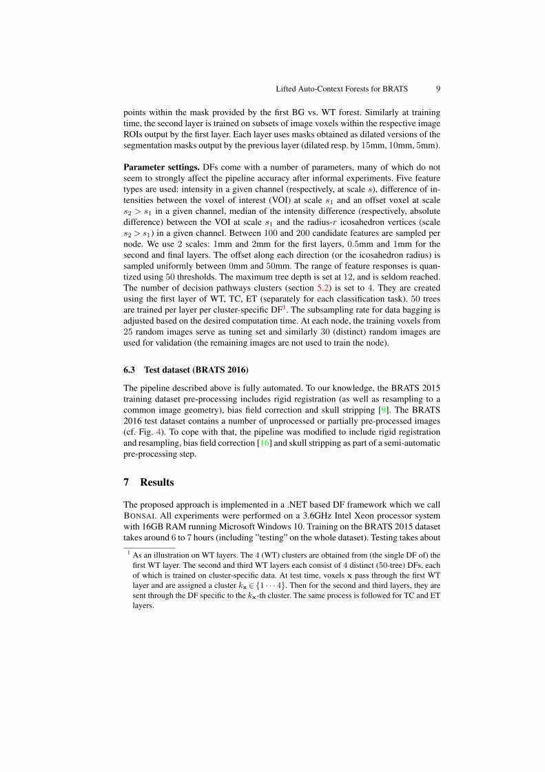
The pipeline described above is fully automated. To our knowledge, the BRATS 2015training dataset pre-processing includes rigid registration (as well as resampling to acommon image geometry), bias field correction and skull stripping [9]. The BRATS2016 test dataset contains a number of unprocessed or partially pre-processed images(cf. Fig. 4). To cope with that, the pipeline was modified to include rigid registrationand resampling, bias field correction [16] and skull stripping as part of a semi-automaticpre-processing step.

7 Results

The proposed approach is implemented in a .NET based DF framework which we callBONSAI. All experiments were performed on a 3.6GHz Intel Xeon processor systemwith 16GB RAM running Microsoft Windows 10. Training on the BRATS 2015 datasettakes around 6 to 7 hours (including ”testing” on the whole dataset). Testing takes about

1 As an illustration on WT layers. The 4 (WT) clusters are obtained from (the single DF of) thefirst WT layer. The second and third WT layers each consist of 4 distinct (50-tree) DFs, eachof which is trained on cluster-specific data. At test time, voxels x pass through the first WTlayer and are assigned a cluster kx ∈{1 · · · 4}. Then for the second and third layers, they aresent through the DF specific to the kx-th cluster. The same process is followed for TC and ETlayers.

10 Le Folgoc et al.

Fig. 4. BRATS 2016 test data: example of variability not seen in the training set. (Left) Bias field,(Middle) Partial skull stripping, (Right) Rigid misalignment, different geometry.

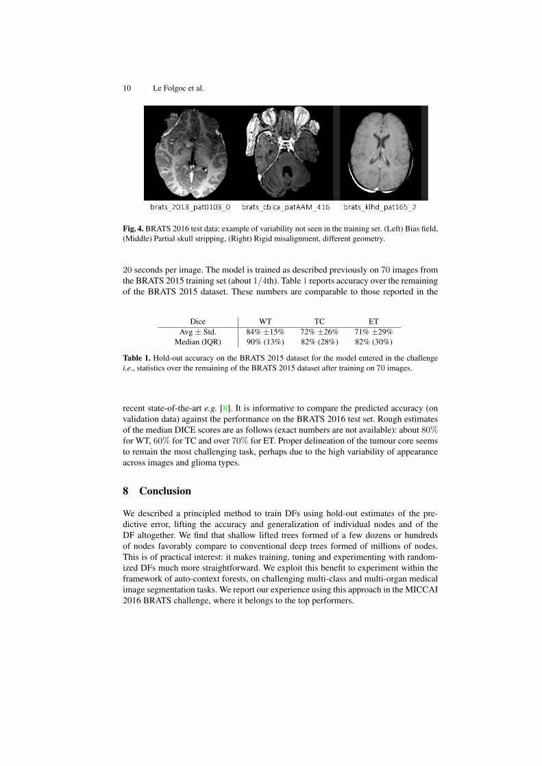
20 seconds per image. The model is trained as described previously on 70 images fromthe BRATS 2015 training set (about 1/4th). Table 1 reports accuracy over the remainingof the BRATS 2015 dataset. These numbers are comparable to those reported in the

Dice WT TC ETAvg ± Std. 84% ±15% 72% ±26% 71% ±29%

Median (IQR) 90% (13%) 82% (28%) 82% (30%)

Table 1. Hold-out accuracy on the BRATS 2015 dataset for the model entered in the challengei.e., statistics over the remaining of the BRATS 2015 dataset after training on 70 images.

recent state-of-the-art e.g. [8]. It is informative to compare the predicted accuracy (onvalidation data) against the performance on the BRATS 2016 test set. Rough estimatesof the median DICE scores are as follows (exact numbers are not available): about 80%for WT, 60% for TC and over 70% for ET. Proper delineation of the tumour core seemsto remain the most challenging task, perhaps due to the high variability of appearanceacross images and glioma types.

8 Conclusion

We described a principled method to train DFs using hold-out estimates of the pre-dictive error, lifting the accuracy and generalization of individual nodes and of theDF altogether. We find that shallow lifted trees formed of a few dozens or hundredsof nodes favorably compare to conventional deep trees formed of millions of nodes.This is of practical interest: it makes training, tuning and experimenting with random-ized DFs much more straightforward. We exploit this benefit to experiment within theframework of auto-context forests, on challenging multi-class and multi-organ medicalimage segmentation tasks. We report our experience using this approach in the MICCAI2016 BRATS challenge, where it belongs to the top performers.

Lifted Auto-Context Forests for BRATS 11

˙Acknowledgment. The authors would like to thank the Microsoft–Inria Joint Centrefor partially funding this work.

References

1. Amit, Y., Geman, D.: Shape quantization and recognition with randomized trees. NeuralComputation 9(7), 1545–1588 (1997) 3

2. Archambeau, C., Verleysen, M.: Robust Bayesian clustering. Neural Networks 20(1), 129–138 (2007) 7

3. Breiman, L.: Bagging predictors. Machine Learning 24(2), 123–140 (1996) 34. Cordier, N., Delingette, H., Ayache, N.: A patch-based approach for the segmentation of

pathologies: application to glioma labelling. IEEE T Med Imaging 35(4) (2015) 85. Criminisi, A., Robertson, D., Konukoglu, E., Shotton, J., Pathak, S., White, S., Siddiqui, K.:

Regression forests for efficient anatomy detection and localization in computed tomographyscans. Medical Image Analysis 17(8), 1293–1303 (2013) 3

6. Geremia, E., Menze, B.H., Ayache, N.: Spatially adaptive random forests. In: 2013 IEEE10th International Symposium on Biomedical Imaging. pp. 1344–1347. IEEE (2013) 1

7. Ho, T.K.: The random subspace method for constructing decision forests. IEEE Trans PatternAnal Mach Intell 20(8), 832–844 (1998) 3

8. Kamnitsas, K., Ledig, C., Newcombe, V.F., Simpson, J.P., Kane, A.D., Menon, D.K., Rueck-ert, D., Glocker, B.: Efficient multi-scale 3D CNN with fully connected CRF for accuratebrain lesion segmentation. arXiv preprint arXiv:1603.05959 (2016) 10

9. Menze, B., Jakab, A., Bauer, S., Kalpathy-Cramer, J., Farahani, K., Kirby, J., Burren, Y.,Porz, N., Slotboom, J., Wiest, R., et al.: The Multimodal Brain Tumor Image SegmentationBenchmark (BRATS). IEEE T Med Imaging 34(10), 1993–2024 (2015) 7, 9

10. Menze, B.H., Van Leemput, K., Lashkari, D., Weber, M.A., Ayache, N., Golland, P.: A gen-erative model for brain tumor segmentation in multi-modal images. In: International Con-ference on Medical Image Computing and Computer-Assisted Intervention. pp. 151–159.Springer (2010) 8

11. Pereira, S., Pinto, A., Alves, V., Silva, C.A.: Deep convolutional neural networks for thesegmentation of gliomas in multi-sequence MRI. In: International Workshop on Brainle-sion: Glioma, Multiple Sclerosis, Stroke and Traumatic Brain Injuries. pp. 131–143. Springer(2015) 1

12. Quinlan, J.R.: Simplifying decision trees. Int J Man Mach Stud 27(3), 221–234 (1987) 513. Shotton, J., Johnson, M., Cipolla, R.: Semantic texton forests for image categorization and

segmentation. In: IEEE Conference on Computer Vision and Pattern Recognition (CVPR),2008. pp. 1–8. IEEE (2008) 1

14. Tu, Z.: Auto-context and its application to high-level vision tasks. In: IEEE Conference onComputer Vision and Pattern Recognition (CVPR), 2008. pp. 1–8. IEEE (2008) 1

15. Tu, Z., Bai, X.: Auto-context and its application to high-level vision tasks and 3D brain imagesegmentation. IEEE Trans Pattern Anal Mach Intell 32(10), 1744–1757 (2010) 1

16. Tustison, N., Gee, J.: N4ITK: Nicks N3 ITK implementation for MRI bias field correction.Insight Journal (2009) 9

17. Tustison, N.J., Shrinidhi, K., Wintermark, M., Durst, C.R., Kandel, B.M., Gee, J.C., Gross-man, M.C., Avants, B.B.: Optimal symmetric multimodal templates and concatenated ran-dom forests for supervised brain tumor segmentation (simplified) with ANTsR. Neuroinfor-matics 13(2), 209–225 (2015) 1

12 Le Folgoc et al.

18. Tustison, N., Wintermark, M., Durst, C., Avants, B.: Ants andarboles. Multimodal BrainTumor Segmentation p. 47 (2013) 1

19. Viola, P., Jones, M.: Rapid object detection using a boosted cascade of simple features. In:Proceedings of the 2001 IEEE Computer Society Conference on Computer Vision and Pat-tern Recognition (CVPR). vol. 1, pp. I–511. IEEE (2001) 3

20. Zhang, Y., Brady, M., Smith, S.: Segmentation of brain MR images through a hidden MarkovRandom Field model and the Expectation-Maximization algorithm. IEEE T Med Imaging20(1), 45–57 (2001) 8

21. Zikic, D., Glocker, B., Konukoglu, E., Criminisi, A., Demiralp, C., Shotton, J., Thomas, O.,Das, T., Jena, R., Price, S.: Decision forests for tissue-specific segmentation of high-gradegliomas in multi-channel MR. In: International Conference on Medical Image Computingand Computer-Assisted Intervention. pp. 369–376. Springer (2012) 1

A BRATS 2015 dataset: training IDs

For completeness, the identifiers of images from the BRATS 2015 dataset that wereused for training (section 6.1) are listed below.

2013 pat0001 1, 2013 pat0002 1, 2013 pat0003 1, 2013 pat0004 1, 2013 pat0005 1,2013 pat0006 1, 2013 pat0007 1, 2013 pat0008 1, 2013 pat0009 1, 2013 pat0010 1,2013 pat0011 1, 2013 pat0012 1, 2013 pat0013 1, 2013 pat0014 1, 2013 pat0015 1,2013 pat0022 1, 2013 pat0024 1, 2013 pat0025 1, 2013 pat0026 1, 2013 pat0027 1,tcia pat105 0001, tcia pat117 0001, tcia pat124 0003, tcia pat133 0001, tcia pat149 0001,tcia pat153 0181, tcia pat165 0001, tcia pat170 0002, tcia pat260 0129, tcia pat260 0244,tcia pat260 0317, tcia pat265 0001, tcia pat290 0580, tcia pat296 0001, tcia pat300 0001,tcia pat314 0001, tcia pat319 0001, tcia pat370 0001, tcia pat372 0001, tcia pat375 0001,tcia pat377 0001, tcia pat396 0139, tcia pat396 0176, tcia pat401 0001, tcia pat430 0001,tcia pat491 0001, 2013 pat0001 1, 2013 pat0004 1, 2013 pat0006 1, 2013 pat0008 1,2013 pat0011 1, 2013 pat0012 1, 2013 pat0013 1, 2013 pat0014 1, 2013 pat0015 1,tcia pat101 0001, tcia pat109 0001, tcia pat141 0001, tcia pat241 0001, tcia pat249 0001,tcia pat298 0001, tcia pat307 0001, tcia pat325 0001, tcia pat346 0001, tcia pat354 0001,tcia pat393 0001, tcia pat402 0001, tcia pat408 0001, tcia pat413 0001, tcia pat442 0001,tcia pat449 0001,