Embed Size (px)
Citation preview
Copyright © 2020 by Modern Scientific Press Company, Florida, USA
International Journal of Modern Mathematical Sciences, 2020, 18(1): 11-30
International Journal of Modern Mathematical Sciences
Journal homepage: www.ModernScientificPress.com/Journals/ijmms.aspx
ISSN: 2166-286X
Florida, USA
Article
Lifting Scheme for the Numerical Solution of Fisher’s Equations
Using Different Wavelet Filter Coefficients
S. C. Shiralashettia*, L. M. Angadib, A. B. Deshic
a Department of Mathematics, Karnatak University Dharwad – 580003, India
b Department of Mathematics, Govt. First Grade College, Chikodi – 591201, India
c Department of Mathematics, KLE CET, Chikodi – 591201, India
*Author to whom correspondence should be addressed; E-Mail:[email protected]
Article history: Received 19 October 2019; Revised 1 February 2020; Accepted 12 February 2020;
Published 20 February 2020.
Abstract: Nonlinear partial differential equations appear in a wide variety of scientific
applications such as plasma physics, solid state physics, optical fibers, biology, fluid
dynamics and chemical kinetics. In this paper, we proposed Lifting scheme for the
numerical solution of Fisher’s equations by different wavelet filter coefficients. The
obtained numerical results using this scheme are compared with the exact solution to reveal the
accuracy and also speed up convergence in lesser computational time as compared with
existing scheme. Some test problems are presented for the applicability and validity of the
schemes.
Keywords: Fisher’s equations; Haar, Daubechies and Biorthogonal wavelet filter
coefficients; Lifting scheme.
AMS Subject Classification: 65T60, 97N40, 46G15, 49K20
1. Introduction
Various phenomena’s in engineering, biology, fluid mechanics and other sciences can be
modeled as both linear and nonlinear partial differential equations (PDEs) [1]. In last decade there has
been much interest for finding the numerical solution of such type of partial differential equations
(PDEs). In general PDEs with or without reaction terms are used as a primary tool to model a broad
Int. J. Modern Math. Sci. 2020, 18(1): 11-30
Copyright © 2020 by Modern Scientific Press Company, Florida, USA
12
class of phenomena occurring in physical and biological sciences, such as Fisher’s equation. This
equation proposed by Fisher in the year 1930 as a model for the propagation of a mutantgene and this
combines diffussion with logistic nonlinearty. Moreover, the same equation occurs in logestic
population growth models, flame propagation, autocatalytic chemical reactions and branching
Brownian motion processes.
In recent times, a number of the iterative methods are used for the numerical and analytical
solutions of linear and nonlinear partial differential equations. Some of them are viz., Adomian
decomposition method [2], He’s variational iteration technique [3] and the homotopy perturbation
method [4], etc. Mathematical models of basic flow equations which express unsteady transport
problems are governed by a single or a system of nonlinear PDEs.
Wavelet analysis assumed significance due to successful applications in signal and image
processing during the 1980s. The smooth orthonormal basis obtained by the translation and dilation of
a single function in a hierarchical fashion proved very valuable to build up compression algorithms for
signals and images up to a selected threshold of relevant amplitudes. Some of the most important
contributors to this theory are: multiresolution signal processing used in computer vision; sub band
coding, developed for speech and image compression; and wavelet series expansion, developed in
applied mathematics.
Some of the previous works on wavelet based methods can be establish in [5-6]. In recent
times a few of the researchers have developed various wavelet based multigrid methods for example:
Daubechies Wavelet based Multigrid and Full Approximation Scheme [7], Biorthogonal wavelet based
full approximation scheme [8] etc. The wavelet based full approximation scheme (WFAS) has
exposed to be a very competent and constructive method for numerous problems associated to
computational science and engineering fields [9]. These methods can be either used as an iterative
solver or as a preconditioning methods, contribution in many cases a better performance than some of
the most new and existing FAS algorithms. Due to the competence and potentiality of WFAS,
researches further have been conceded out for its improvement. In order to understand this task, work
build that is orthogonal/biorthogonal discrete wavelet transform by lifting scheme [10]. Sweldens is
introduced wavelet based lifting technique [11], which permits several improvements on the properties
of existing wavelet transforms. The technique has some numerical benefits as a reduced number of
operations which are essential in the context of the iterative solvers. Obviously all attempts to shorten
the wavelet solutions for PDE are welcome. In PDE, matrices arising from system are intense with
non-smooth diagonal and smooth away from the diagonal. This efficiency of the matrix transforms into
compactness using wavelet transform and it leads to propose the effective lifting scheme using
differernt wavelets.
Int. J. Modern Math. Sci. 2020, 18(1): 11-30
Copyright © 2020 by Modern Scientific Press Company, Florida, USA
13
Lifting scheme is a new approach to build the so-called second generation wavelets that are not
necessarily translations and dilations of one function. The latter we refer to as a first generation
wavelets or classical methods. The lifting scheme has some additional advantages in association with
the classical wavelets. This transform works for signals of an arbitrary size with accurate treatment of
boundaries. A further characteristic of the lifting scheme is that all constructions are resulting in the
spatial domain. This is in distinction to the conventional approach, which relies deeply on the
frequency domain. The two most important advantageous are:
i. It leads to a more intuitively appealing treatment improved suited to those in attracted in
applications than mathematical foundations.
ii. It makes a computational time most favorable and from time to time increasing the speed of
calculations.
The lifting scheme starts with a set of well-known filters, subsequently lifting steps are used an
effort to improve (lift) the properties of an equivalent wavelet decomposition. This process has a few
mathematical benefits as a condensed number of operations which are crucial in the circumstance of
the iterative solvers. In addition to this, the current paper illustrates that the relevance of the lifting
scheme using different wavelets for the numerical solution of Fisher’s equations.
The present paper is organized as follows: In section 2, Preliminaries of wavelet filter coefficients and
lifting scheme. The method of solution describes in section 3. In section 4 provides numerical
simulation of test problems and finally, in section 5 conclusion of the proposed work is given.
2. Preliminaries of Wavelet Filter Coefficients and Lifting Scheme
The lifting scheme starts with a set of familiar filters; thereafter lifting steps are used in attempt
to advance the properties of corresponding wavelet decomposition.
Now, we have discussed about different wavelet filters as follows:
2.1. Haar Wavelet Filter Coefficients
We are familiar with that of low pass filter coefficients 0 1
1 1, ,
2 2
T
Ta a
and high pass
filter coefficients 0 1
1 1, ,
2 2
T
Tb b
play a significant role in decomposition. Thus it is natural to
wonder that it achievable to model the decomposition in terms of linear transformations i.e. matrices.
Furthermore, while digital signals and images are composed of discrete data, we want to discrete
analog of the decomposition algorithm so that we can process signal and image data.
Int. J. Modern Math. Sci. 2020, 18(1): 11-30
Copyright © 2020 by Modern Scientific Press Company, Florida, USA
14
2.2. Daubechies Wavelet Filter Coefficients
Daubechies introduced scaling functions having the shortest feasible support. The scaling
function N has support 0, 1N , while the equivalent wavelet
N has carry in the
interval 1 / 2, / 2N N .
For Daubechies wavelets, the low pass filter coefficients
0 1 2 3
1 3 3 3 3 3 1 3
4 2 4 2 4 2 4 2, , , , , ,
T
Ta a a a
and high pass filter coefficients 0 1 2 3
1 3 3 3 3 3 1 3
4 2 4 2 4 2 4 2, , , , , ,
T
Tb b b b
2.3. Biorthogonal (CDF (2,2)) Wavelets
Let’s consider the (5, 3) biorthogonal spline wavelet filter pair, the low pass filter pair are
1 0 1
1 1 1( , , ) , ,
2 2 2 2 2a a a
and 2 1 0 1 2
1 1 3 1 1( , , , , ) , , , ,
4 2 2 2 2 2 2 2 4 2a a a a a
.
But, we have 1 1( 1) and ( 1)k k
k k k kb a b a ,
the high pass filter pair are
0 1 2
1 1 1, ,
2 2 2 2 2b b b
&
1 0 1 2 3
1 1 3 1 1, , , ,
4 2 2 2 2 2 2 2 4 2b b b b b
2.4. Foundations of Lifting Scheme
Consider to numbers a, b as two neighbouring samples of a sequence and then these have
some correlation which we would like to take advantage. The simple linear transform which replaces a
and b by average s and difference d i.e.
&2 2
a b a bs d
The idea is that if a and b are highly correlated, the expected absolute value of their difference
d will be small and can be represented with fever bits. In case that a = b, the difference is simply zero.
We have not lost any information because we can always recover a and b from the gives s and d as:
&2 2
d da s b s
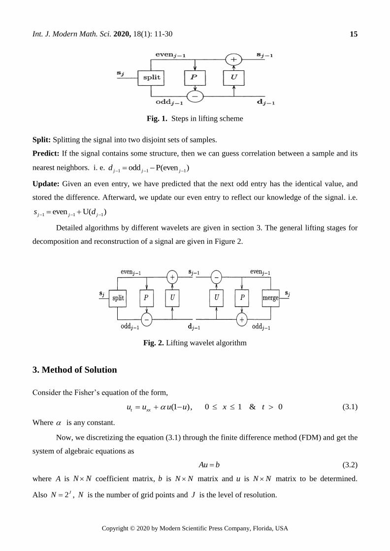
Finally, a wavelet transform built through lifting consists of three steps: split. Predict and
update as given in the Figure 1 [12]
Int. J. Modern Math. Sci. 2020, 18(1): 11-30
Copyright © 2020 by Modern Scientific Press Company, Florida, USA
15
Fig. 1. Steps in lifting scheme
Split: Splitting the signal into two disjoint sets of samples.
Predict: If the signal contains some structure, then we can guess correlation between a sample and its
nearest neighbors. i. e. 1 1 1odd P(even )j j jd
Update: Given an even entry, we have predicted that the next odd entry has the identical value, and
stored the difference. Afterward, we update our even entry to reflect our knowledge of the signal. i.e.
1 1 1even U( )j j js d
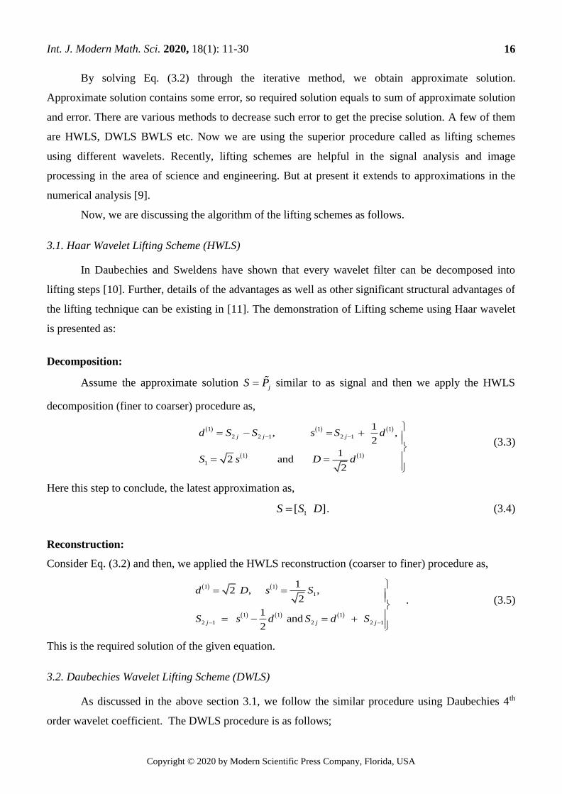
Detailed algorithms by different wavelets are given in section 3. The general lifting stages for
decomposition and reconstruction of a signal are given in Figure 2.
Fig. 2. Lifting wavelet algorithm
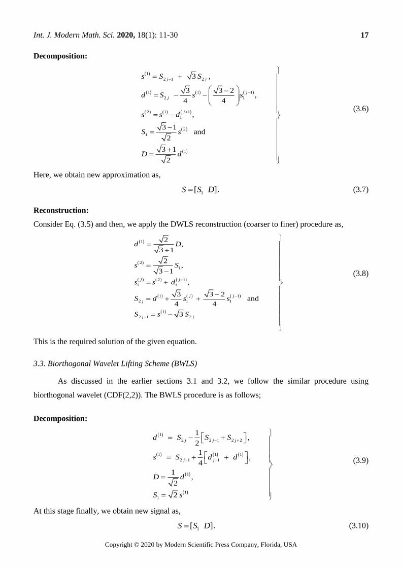
3. Method of Solution
Consider the Fisher’s equation of the form,
(1 ), 0 1 & 0t xxu u u u x t (3.1)
Where is any constant.
Now, we discretizing the equation (3.1) through the finite difference method (FDM) and get the
system of algebraic equations as
Au b (3.2)
where A is N N coefficient matrix, b is N N matrix and u is N N matrix to be determined.
Also 2JN , N is the number of grid points and J is the level of resolution.
Int. J. Modern Math. Sci. 2020, 18(1): 11-30
Copyright © 2020 by Modern Scientific Press Company, Florida, USA
16
By solving Eq. (3.2) through the iterative method, we obtain approximate solution.
Approximate solution contains some error, so required solution equals to sum of approximate solution
and error. There are various methods to decrease such error to get the precise solution. A few of them
are HWLS, DWLS BWLS etc. Now we are using the superior procedure called as lifting schemes
using different wavelets. Recently, lifting schemes are helpful in the signal analysis and image
processing in the area of science and engineering. But at present it extends to approximations in the
numerical analysis [9].
Now, we are discussing the algorithm of the lifting schemes as follows.
3.1. Haar Wavelet Lifting Scheme (HWLS)
In Daubechies and Sweldens have shown that every wavelet filter can be decomposed into
lifting steps [10]. Further, details of the advantages as well as other significant structural advantages of
the lifting technique can be existing in [11]. The demonstration of Lifting scheme using Haar wavelet
is presented as:
Decomposition:
Assume the approximate solution jS P similar to as signal and then we apply the HWLS
decomposition (finer to coarser) procedure as,
1 1 1
2 2 1 2 1
1 1
1
1, ,
2
12 and
2
j j jd S S s S d
S s D d
(3.3)
Here this step to conclude, the latest approximation as,
1[ ]S S D . (3.4)
Reconstruction:
Consider Eq. (3.2) and then, we applied the HWLS reconstruction (coarser to finer) procedure as,
1 1
1
1 1 1
2 1 2 2 1
12 , ,
2
1and
2j j j
d D s S
S s d S d S
. (3.5)
This is the required solution of the given equation.
3.2. Daubechies Wavelet Lifting Scheme (DWLS)
As discussed in the above section 3.1, we follow the similar procedure using Daubechies 4th
order wavelet coefficient. The DWLS procedure is as follows;
Int. J. Modern Math. Sci. 2020, 18(1): 11-30
Copyright © 2020 by Modern Scientific Press Company, Florida, USA
17
Decomposition:
1
2 1 2
1 1 1
2 1
2 1 1
1
2
1
1
3 ,
3 3 2,
4 4
,
3 1and
2
3 1
2
j j
j
j
j
s S S
d S s s
s s d
S s
D d
(3.6)
Here, we obtain new approximation as,
1[ ]S S D . (3.7)
Reconstruction:
Consider Eq. (3.5) and then, we apply the DWLS reconstruction (coarser to finer) procedure as,
1
2
1
2 1
1 1
1 1
2 1 1
1
2 1 2
2,
3 1
2,
3 1
,
3 3 2and
4 4
3
j j
j j
j
j j
d D
s S
s s d
S d s s
S s S
(3.8)
This is the required solution of the given equation.
3.3. Biorthogonal Wavelet Lifting Scheme (BWLS)
As discussed in the earlier sections 3.1 and 3.2, we follow the similar procedure using
biorthogonal wavelet (CDF(2,2)). The BWLS procedure is as follows;
Decomposition:
1
2 2 1 2 2
1 1 1
2 1 1
1
1
1
1,
2
1,
4
1,
2
2
j j j
j j
d S S S
s S d d
D d
S s
(3.9)
At this stage finally, we obtain new signal as,
1[ ]S S D . (3.10)
Int. J. Modern Math. Sci. 2020, 18(1): 11-30
Copyright © 2020 by Modern Scientific Press Company, Florida, USA
18
Reconstruction:
Consider Eqn. (3.10) and then, we apply the DWLS reconstruction (coarser to finer) procedure as
1
1
1
1 1 1
2 1 1
1
2 2 1 2 2
1,
2
2 ,
1
4
1) ,
2
j j
j j j
s S
d D
S s d d
S d S S
(3.11)
This is the required solution of the given equation.
The coefficients 1
js and
1
jd are the average and thorough coefficients respectively of the
approximate solution au . The new approaches are tested through a variety of problems and the results
are revealed in section 4.
4. Numerical Simulation
In this section, we applied Lifting scheme for the numerical solution of Fisher’s equation and
also show the applicability and competence of HWLS, DWLS and BWLS. The error is computed by
maxma x e au uE , where eu and au are exact and approximate solution respectively.
Test Problem 4.1: Now, we consider the Fisher equation
6 (1 ), 0 1 & 0t xxu u u u x t (4.1.1)
subject to the I.C.: 21
10,xe
xu
(4.1.2)
and B.C.s: 251
1,0te
tu
, 2)51(1
1,1te
tu
(4.1.3)
Which has the exact solution 2)5(1
1,txe
txu
[13].
Now discretizing the Eq. (4.1.1) by using finite difference scheme,
1
1 1
2
26 1
j j jj ji i i j ji i
i i
u u uu uu u
h h
(4.1.4)
1 2
1 12 6 1j j j j j j j
i i i i i i ih u u u u u h u u
, , 1, 2,....i j N .
1
1 1 1 6 2 0j j j j j
i i i i iu u hu u h h hu
(4.1.5)
, 0F i j (4.1.6)

Int. J. Modern Math. Sci. 2020, 18(1): 11-30
Copyright © 2020 by Modern Scientific Press Company, Florida, USA
19
Where 1, 1 6 2
1 1jj j j j
F i j u u hu u h h hui i ii i
Which is the system of nonlinear equations, have N N equations with N N unknowns. Solving
Eq. (4.1.6) through the Gauss Seidel iterative method for 4N , we get approximate solution v for u
i.e.
0.486 0.730 0.876 0.948
0.435 0.685 0.848 0.934
0.380 0.639 0.822 0.922
0.319 0.589 0.797 0.913
u
The wavelet based numerical solutions of Eq. (4.1.1) are obtained as per the procedure
explained in section 3 and are as follows,
Assume S u , then apply the HWLS as explained in section 3.1 as,
Decomposition:
1
16 15d S S ,
10.243 0.072 0.250 0.085 0.259 0.100 0.270 0.115d .
1
1
152
ds S ,
10.608 0.912 0.560 0.891 0.509 0.872 0.454 0.855s .
1
1 2S s .
1 0.860 1.290 0.792 1.260 0.720 1.233 0.642 1.209S .
11
2D d .
0.172 0.051 0.177 0.060 0.183 0.071 0.191 0.081D
Reconstruction:
Then apply the HWLS reconstruction procedure as,
12d D ,
10.243 0.072 0.250 0.085 0.259 0.100 0.270 0.115d .
1
1
1
2s S ,
10.608 0.912 0.560 0.891 0.509 0.872 0.454 0.855s .
1 1
15
1
2S s d ,
15 0.486 0.876 0.435 0.848 0.380 0.822 0.319 0.797S .
1
16 15S d S ,
16 0.730 0.948 0.685 0.934 0.639 0.922 0.589 0.913S .
Int. J. Modern Math. Sci. 2020, 18(1): 11-30
Copyright © 2020 by Modern Scientific Press Company, Florida, USA
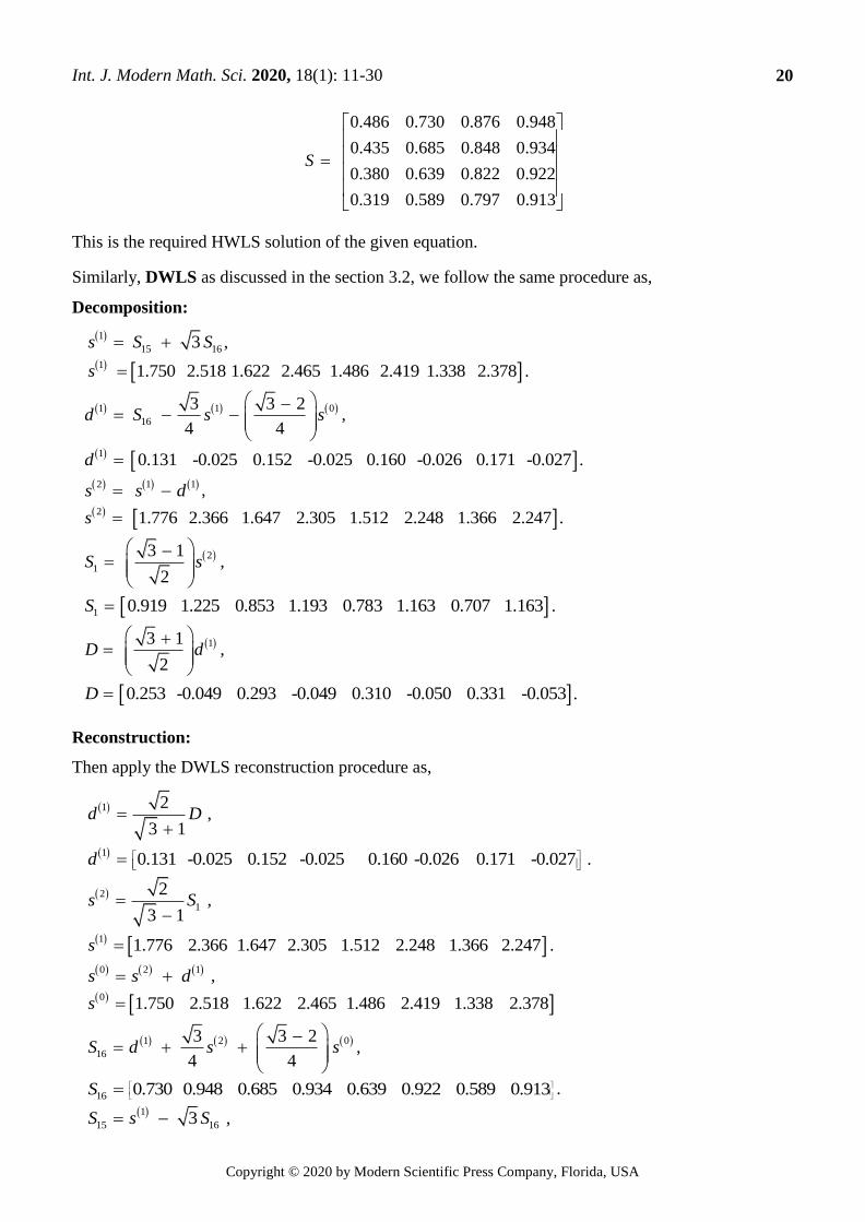
20
0.486 0.730 0.876 0.948
0.435 0.685 0.848 0.934
0.380 0.639 0.822 0.922
0.319 0.589 0.797 0.913
S
This is the required HWLS solution of the given equation.
Similarly, DWLS as discussed in the section 3.2, we follow the same procedure as,
Decomposition:
1
15 163s S S ,
11.750 2.518 1.622 2.465 1.486 2.419 1 .338 2.378s .
1 1 0
16
3 3 2
4 4d S s s
,
10.131 -0.025 0.152 -0.025 0.160 -0.026 0.171 -0.027d .
2 1 1s s d , 2
1.776 2.366 1 .647 2.305 1 .512 2.248 1 .366 2.247s .
2
1
3 1
2S s
,
1 0.919 1 .225 0.853 1 .193 0.783 1 .163 0.707 1 .163S .
13 1
2D d
,
0.253 -0.049 0.293 -0.049 0.310 -0.050 0.331 -0.053D .
Reconstruction:
Then apply the DWLS reconstruction procedure as,
1 2
3 1d D
,
10.131 -0.025 0.152 -0.025 0.160 -0.026 0.171 -0.027d
.
2
1
2
3 1s S
,
11.776 2.366 1 .647 2.305 1 .512 2.248 1 .366 2.247s .
0 2 1s s d , 0
1.750 2.518 1 .622 2.465 1 .486 2.419 1 .338 2.378s
1 2 0
16
3 3 2
4 4S d s s
,
16 0.730 0.948 0.685 0.934 0.639 0.922 0.589 0.913S
.
1
15 163S s S ,
Int. J. Modern Math. Sci. 2020, 18(1): 11-30
Copyright © 2020 by Modern Scientific Press Company, Florida, USA
21
15 0.486 0.876 0.435 0.848 0.380 0.822 0.319 0.797S
.
0.486 0.730 0.876 0.948
0.435 0.685 0.848 0.934
0.380 0.639 0.822 0.922
0.319 0.589 0.797 0.913
S
This is the required DWLS solution of the given equation.
And also, BWLS is explained in the section 3.3, we follow the similar procedure as follows
Decomposition:
1
16 15 17
1,
2d S S S
10.144 0.043 0.148 0.049 0.154 0.054 0.064 0.040d
. 1 1 1
15 0
1
4s S d d ,
10.532 0.923 0.483 0.897 0.431 0.874 0.348 0.824s .
11
2D d ,
0.102 0.030 0.105 0.034 0.109 0.039 0.046 0.028D .
1
1 2S s ,
1 0.753 1 .305 0.683 1 .269 0.609 1 .236 0.493 1 .165S
Reconstruction:
Then apply the BWLS reconstruction procedure as,
1
1
1
2s S ,
10.532 0.923 0.483 0.897 0.431 0.874 0.348 0.824s .
12d D ,
10.144 0.043 0.148 0.049 0.154 0.054 0.064 0.040d
.
1 1 1
15 0
1
4S s d d ,
15 0.486 0.876 0.435 0.848 0.380 0.822 0.319 0.797S .
1
16 15 18
1
4S d S S ,
16 0.730 0.948 0.685 0.934 0.639 0.922 0.589 0.913S .
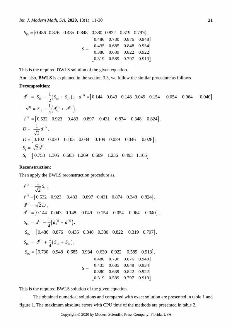
0.486 0.730 0.876 0.948
0.435 0.685 0.848 0.934
0.380 0.639 0.822 0.922
0.319 0.589 0.797 0.913
S
This is the required BWLS solution of the given equation.
The obtained numerical solutions and compared with exact solution are presented in table 1 and
figure 1. The maximum absolute errors with CPU time of the methods are presented in table 2.
Int. J. Modern Math. Sci. 2020, 18(1): 11-30
Copyright © 2020 by Modern Scientific Press Company, Florida, USA
22
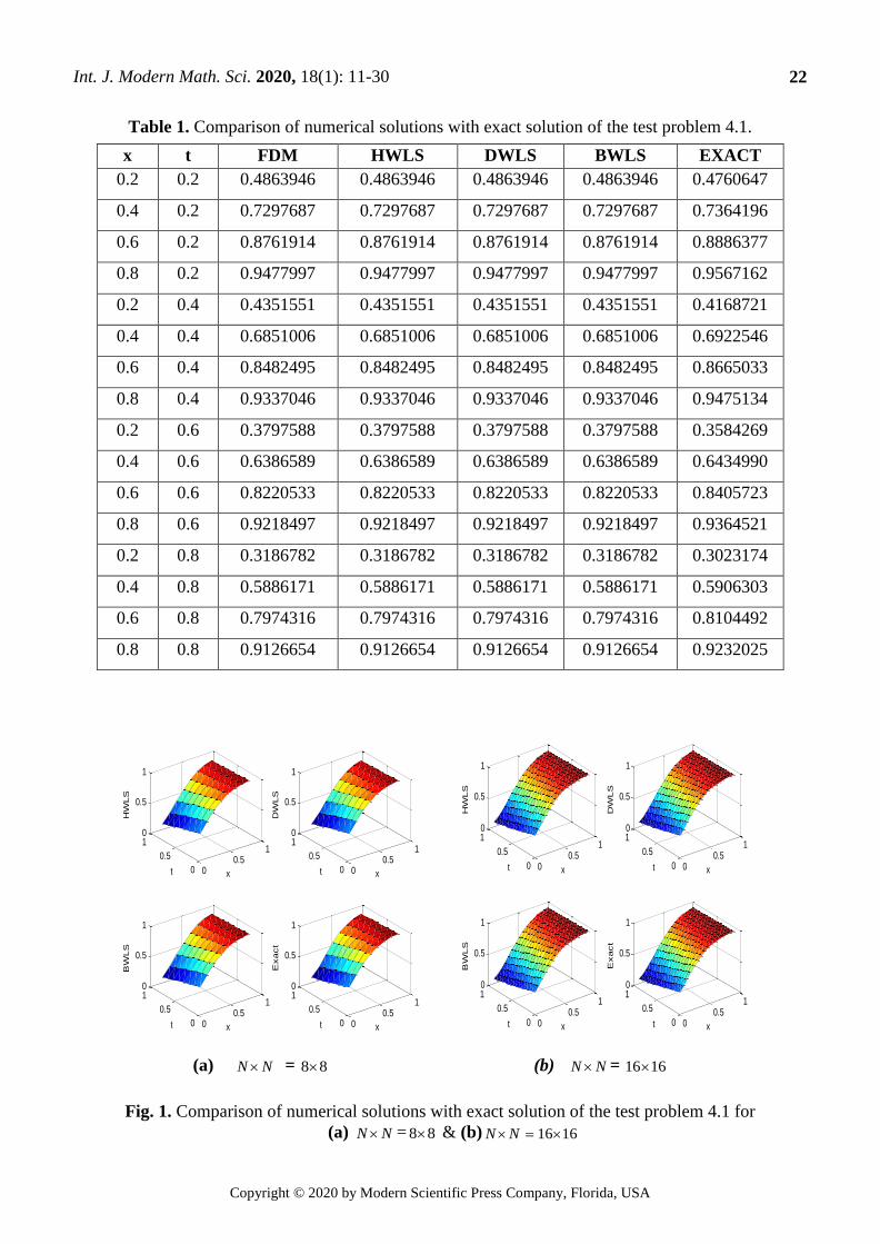
Table 1. Comparison of numerical solutions with exact solution of the test problem 4.1.
00.5
1
0
0.5
10
0.5
1
xt
HW
LS
00.5
1
0
0.5
10
0.5
1
xt
DW
LS
00.5
1
0
0.5
10
0.5
1
xt
BW
LS
00.5
1
0
0.5
10
0.5
1
xt
Exact
00.5
1
0
0.5
10
0.5
1
xt
HW
LS
00.5
1
0
0.5
10
0.5
1
xt
DW
LS
00.5
1
0
0.5
10
0.5
1
xt
BW
LS
00.5
1
0
0.5
10
0.5
1
xt
Exact
(a) N N = 8 8 (b) N N = 16 16
Fig. 1. Comparison of numerical solutions with exact solution of the test problem 4.1 for
(a) N N =8 8 & (b) 16 16N N
x t FDM HWLS DWLS BWLS EXACT
0.2 0.2 0.4863946 0.4863946 0.4863946 0.4863946 0.4760647
0.4 0.2 0.7297687 0.7297687 0.7297687 0.7297687 0.7364196
0.6 0.2 0.8761914 0.8761914 0.8761914 0.8761914 0.8886377
0.8 0.2 0.9477997 0.9477997 0.9477997 0.9477997 0.9567162
0.2 0.4 0.4351551 0.4351551 0.4351551 0.4351551 0.4168721
0.4 0.4 0.6851006 0.6851006 0.6851006 0.6851006 0.6922546
0.6 0.4 0.8482495 0.8482495 0.8482495 0.8482495 0.8665033
0.8 0.4 0.9337046 0.9337046 0.9337046 0.9337046 0.9475134
0.2 0.6 0.3797588 0.3797588 0.3797588 0.3797588 0.3584269
0.4 0.6 0.6386589 0.6386589 0.6386589 0.6386589 0.6434990
0.6 0.6 0.8220533 0.8220533 0.8220533 0.8220533 0.8405723
0.8 0.6 0.9218497 0.9218497 0.9218497 0.9218497 0.9364521
0.2 0.8 0.3186782 0.3186782 0.3186782 0.3186782 0.3023174
0.4 0.8 0.5886171 0.5886171 0.5886171 0.5886171 0.5906303
0.6 0.8 0.7974316 0.7974316 0.7974316 0.7974316 0.8104492
0.8 0.8 0.9126654 0.9126654 0.9126654 0.9126654 0.9232025
Int. J. Modern Math. Sci. 2020, 18(1): 11-30
Copyright © 2020 by Modern Scientific Press Company, Florida, USA
23
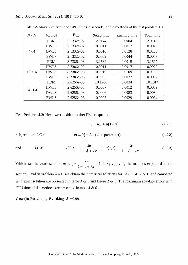
Table 2. Maximum error and CPU time (in seconds) of the methods of the test problem 4.1
Test Problem 4.2: Next, we consider another Fisher equation
1t xxu u u u (4.2.1)
subject to the I.C.: ,0u x ( is parameter) (4.2.2)
and B.C.s: 0,1
t
t
eu t
e
, 1,
1
t
t
eu t
e
(4.2.3)
Which has the exact solution ,1
t
t
eu x t
e[14]. By applying the methods explained in the
section 3 and in problem 4.4.1, we obtain the numerical solutions for 1 & 1 and compared
with exact solution are presented in table 3 & 5 and figure 2 & 3. The maximum absolute errors with
CPU time of the methods are presented in table 4 & 6.
Case (i): For 1 , By taking 0.99
N N Method maxE Setup time Running time Total time
4 4
FDM 2.1332e-02 2.9144 0.0004 2.9148
HWLS 2.1332e-02 0.0011 0.0017 0.0028
DWLS 2.1332e-02 0.0010 0.0128 0.0138
BWLS 2.1332e-02 0.0009 0.0044 0.0053
16 16
FDM 8.7386e-03 3.2582 0.0015 3.2597
HWLS 8.7386e-03 0.0011 0.0017 0.0028
DWLS 8.7386e-03 0.0010 0.0109 0.0119
BWLS 8.7386e-03 0.0005 0.0027 0.0032
64 64
FDM 2.6256e-03 10.1280 0.0034 10.1314
HWLS 2.6256e-03 0.0007 0.0012 0.0019
DWLS 2.6256e-03 0.0006 0.0083 0.0089
BWLS 2.6256e-03 0.0005 0.0029 0.0034

Int. J. Modern Math. Sci. 2020, 18(1): 11-30
Copyright © 2020 by Modern Scientific Press Company, Florida, USA
24
Table 3. Comparison of numerical solutions with exact solution of the test problem 4.2.
(a) N N = 8 8 (b) N N = 16 16
Fig. 2. Comparison of numerical solutions with exact solution of the test problem 4.2 for
(a) N N =8 8 & (b) 16 16N N
x t FDM HWLS DWLS BWLS EXACT
0.2 0.2 0.99172 0.99172 0.99172 0.99172 0.99810
0.4 0.2 0.99171 0.99171 0.99171 0.99171 0.99810
0.6 0.2 0.99170 0.99170 0.99170 0.99171 0.99810
0.8 0.2 0.99174 0.99174 0.99174 0.99174 0.99810
0.2 0.4 0.99311 0.99311 0.99311 0.99311 0.99327
0.4 0.4 0.99307 0.99307 0.99307 0.99307 0.99327
0.6 0.4 0.99310 0.99310 0.99310 0.99310 0.99327
0.8 0.4 0.99318 0.99318 0.99318 0.99318 0.99327
0.2 0.6 0.99421 0.99421 0.99421 0.99421 0.99449
0.4 0.6 0.99414 0.99414 0.99414 0.99414 0.99449
0.6 0.6 0.99421 0.99421 0.99421 0.99421 0.99449
0.8 0.6 0.99435 0.99435 0.99435 0.99435 0.99449
0.2 0.8 0.99508 0.99508 0.99508 0.99508 0.99548
0.4 0.8 0.99498 0.99498 0.99498 0.99498 0.99548
0.6 0.8 0.99509 0.99509 0.99509 0.99509 0.99548
0.8 0.8 0.99529 0.99529 0.99529 0.99529 0.99548

Int. J. Modern Math. Sci. 2020, 18(1): 11-30
Copyright © 2020 by Modern Scientific Press Company, Florida, USA
25
Table 4. Maximum error and CPU time (in seconds) of the methods of the test problem 4.2.
Case (ii): For 1 , By taking 1.1
Table 5. Comparison of numerical solutions with exact solution of test problem 4.2
N N Method maxE Setup time Running time Total time
4 4
FDM 4.9756e-04 2.7199 0.0009 2.7208
HWLS 4.9756e-04 0.0115 0.0040 0.0155
DWLS 4.9756e-04 0.0021 0.0703 0.0724
BWLS 4.9756e-04 0.0038 0.0157 0.0195
16 16
FDM 6.3353e-05 3.9130 0.0021 3.9151
HWLS 6.3353e-05 0.0024 0.0038 0.0062
DWLS 6.3353e-05 0.0020 0.0212 0.0232
BWLS 6.3353e-05 0.0018 0.0092 0.0110
64 64
FDM 2.3252e-05 1.0344 0.0065 1.0409
HWLS 2.3252e-05 0.0024 0.0040 0.0064
DWLS 2.3252e-05 0.0021 0.0212 0.0233
BWLS 2.3252e-05 0.0018 0.0094 0.0112
x t FDM HWLS DWLS BWLS EXACT
0.2 0.2 1.0809 1.0809 1.0809 1.0809 1.0804
0.4 0.2 1.0812 1.0812 1.0812 1.0812 1.0804
0.6 0.2 1.0812 1.0812 1.0812 1.0812 1.0804
0.8 0.2 1.0810 1.0810 1.0810 1.0810 1.0804
0.2 0.4 1.0654 1.0654 1.0654 1.0654 1.0649
0.4 0.4 1.0656 1.0656 1.0656 1.0656 1.0649
0.6 0.4 1.0657 1.0657 1.0657 1.0657 1.0649
0.8 0.4 1.0654 1.0654 1.0654 1.0654 1.0649
0.2 0.6 1.0528 1.0528 1.0528 1.0528 1.0525
0.4 0.6 1.0530 1.0530 1.0530 1.0530 1.0525
0.6 0.6 1.0531 1.0531 1.0531 1.0531 1.0525
0.8 0.6 1.0529 1.0529 1.0529 1.0529 1.0525
0.2 0.8 1.0427 1.0427 1.0427 1.0427 1.0426
0.4 0.8 1.0428 1.0428 1.0428 1.0428 1.0426
0.6 0.8 1.0429 1.0429 1.0429 1.0429 1.0426
0.8 0.8 1.0429 1.0429 1.0429 1.0429 1.0426
Int. J. Modern Math. Sci. 2020, 18(1): 11-30
Copyright © 2020 by Modern Scientific Press Company, Florida, USA
26
(a) N N = 8 8 (b) N N = 16 16
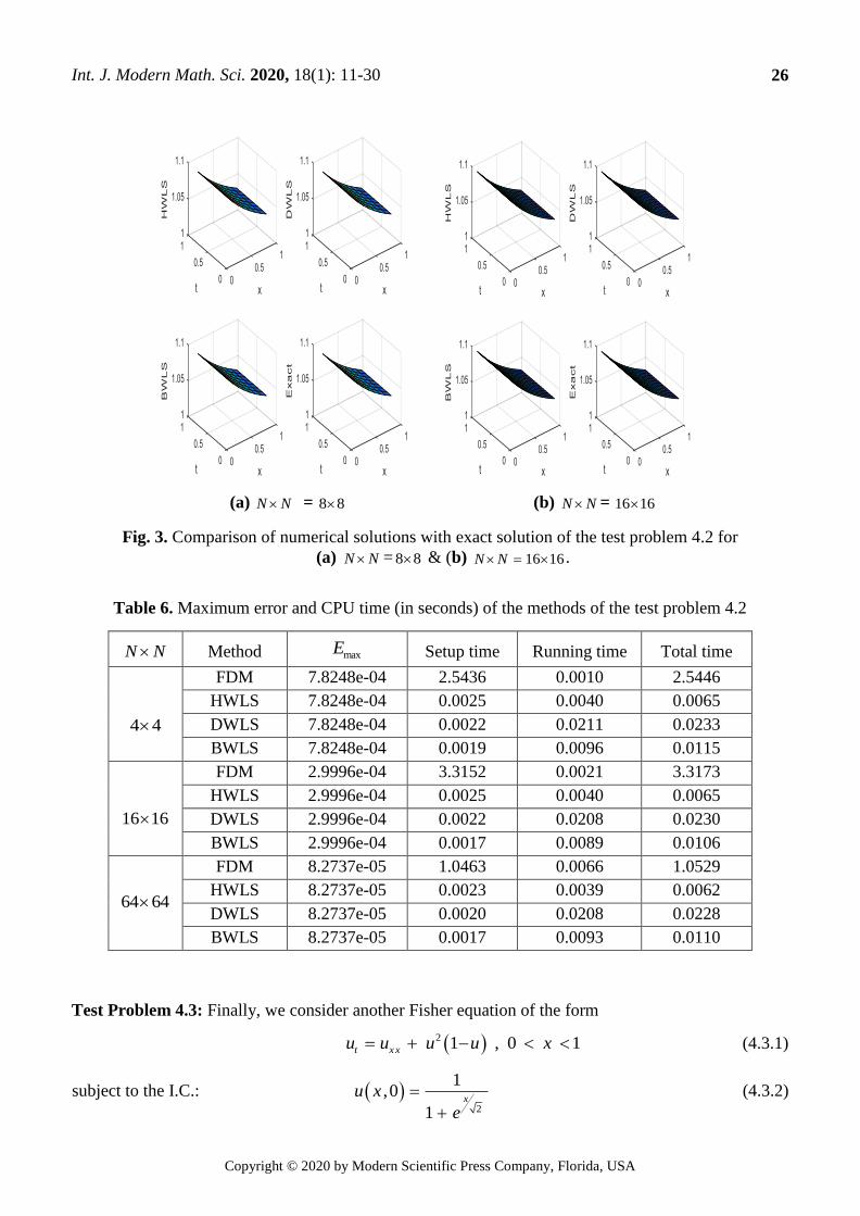
Fig. 3. Comparison of numerical solutions with exact solution of the test problem 4.2 for
(a) N N =8 8 & (b) 16 16N N .
Table 6. Maximum error and CPU time (in seconds) of the methods of the test problem 4.2
Test Problem 4.3: Finally, we consider another Fisher equation of the form
2 1 , 0 1t x xu u u u x (4.3.1)
subject to the I.C.: 2
1,0
1x
u x
e
(4.3.2)
N N Method maxE Setup time Running time Total time
4 4
FDM 7.8248e-04 2.5436 0.0010 2.5446
HWLS 7.8248e-04 0.0025 0.0040 0.0065
DWLS 7.8248e-04 0.0022 0.0211 0.0233
BWLS 7.8248e-04 0.0019 0.0096 0.0115
16 16
FDM 2.9996e-04 3.3152 0.0021 3.3173
HWLS 2.9996e-04 0.0025 0.0040 0.0065
DWLS 2.9996e-04 0.0022 0.0208 0.0230
BWLS 2.9996e-04 0.0017 0.0089 0.0106
64 64
FDM 8.2737e-05 1.0463 0.0066 1.0529
HWLS 8.2737e-05 0.0023 0.0039 0.0062
DWLS 8.2737e-05 0.0020 0.0208 0.0228
BWLS 8.2737e-05 0.0017 0.0093 0.0110
Int. J. Modern Math. Sci. 2020, 18(1): 11-30
Copyright © 2020 by Modern Scientific Press Company, Florida, USA
27
and B.C.s: 2
10,
1t
u t
e
, 1 1
12 2
11,
1t
u t
e
(4.3.3)
Which has the exact solution 1 1
2 2
1( , )
1x t
u x t
e
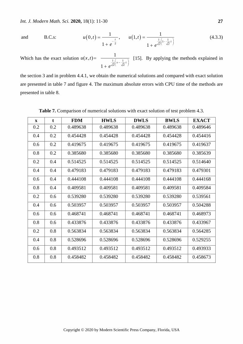
[15]. By applying the methods explained in
the section 3 and in problem 4.4.1, we obtain the numerical solutions and compared with exact solution
are presented in table 7 and figure 4. The maximum absolute errors with CPU time of the methods are
presented in table 8.
Table 7. Comparison of numerical solutions with exact solution of test problem 4.3.
x t FDM HWLS DWLS BWLS EXACT
0.2 0.2 0.489638 0.489638 0.489638 0.489638 0.489646
0.4 0.2 0.454428 0.454428 0.454428 0.454428 0.454416
0.6 0.2 0.419675 0.419675 0.419675 0.419675 0.419637
0.8 0.2 0.385680 0.385680 0.385680 0.385680 0.385639
0.2 0.4 0.514525 0.514525 0.514525 0.514525 0.514640
0.4 0.4 0.479183 0.479183 0.479183 0.479183 0.479301
0.6 0.4 0.444108 0.444108 0.444108 0.444108 0.444168
0.8 0.4 0.409581 0.409581 0.409581 0.409581 0.409584
0.2 0.6 0.539280 0.539280 0.539280 0.539280 0.539561
0.4 0.6 0.503957 0.503957 0.503957 0.503957 0.504288
0.6 0.6 0.468741 0.468741 0.468741 0.468741 0.468973
0.8 0.6 0.433876 0.433876 0.433876 0.433876 0.433967
0.2 0.8 0.563834 0.563834 0.563834 0.563834 0.564285
0.4 0.8 0.528696 0.528696 0.528696 0.528696 0.529255
0.6 0.8 0.493512 0.493512 0.493512 0.493512 0.493933
0.8 0.8 0.458482 0.458482 0.458482 0.458482 0.458673

Int. J. Modern Math. Sci. 2020, 18(1): 11-30
Copyright © 2020 by Modern Scientific Press Company, Florida, USA
28
00.5
1
0
0.5
10
0.5
1
xt
HW
LS
00.5
1
0
0.5
10
0.5
1
xt
DW
LS
00.5
1
0
0.5
10
0.5
1
xt
BW
LS
00.5
1
0
0.5
10
0.5
1
xt
Exact
00.5
1
0
0.5
10
0.5
1
xt
HW
LS
00.5
1
0
0.5
10
0.5
1
xt
DW
LS
00.5
1
0
0.5
10
0.5
1
xt
BW
LS
00.5
1
0
0.5
10
0.5
1
xt
Exact
(a) N N = 8 8 (b) N N = 16 16
Fig. 4. Comparison of numerical solutions with exact solution of the test problem 4.3 for
(a) N N =8 8 & (b) 16 16N N
Table 8. Maximum error and CPU time (in seconds) of the methods of the test problem 4.3.
N N Method maxE Setup time Running time Total time
4 4
FDM 5.5899e-04 2.7258 0.0003 2.7261
HWLS 5.5899e-04 0.0007 0.0010 0.0017
DWLS 5.5899e-04 0.0008 0.0127 0.0135
BWLS 5.5899e-04 0.0007 0.0043 0.0050
16 16
FDM 6.7437e-05 2.7272 0.0015 2.7287
HWLS 6.7437e-05 0.0010 0.0016 0.0026
DWLS 6.7437e-05 0.0008 0.0089 0.0097
BWLS 6.7437e-05 0.0005 0.0027 0.0032
64 64
FDM 2.8217e-05 10.0350 0.0035 10.0385
HWLS 2.8217e-05 0.0007 0.0011 0.0018
DWLS 2.8217e-05 0.0005 0.0084 0.0089
BWLS 2.8217e-05 0.0005 0.0029 0.0034
Int. J. Modern Math. Sci. 2020, 18(1): 11-30
Copyright © 2020 by Modern Scientific Press Company, Florida, USA
29
5. Conclusions
In this paper, we applied the Lifting scheme for the numerical solution of Fisher’s equations
using different wavelet filters coefficients. From the figures we observed that the numerical solutions
obtained by different Lifting schemes are agrees with the exact solution. Furthermore, in the tables the
convergence of the presented schemes i.e. the error decreases when the level of resolution N increases.
In addition to this, the calculations involved in Lifting schemes are simple, straight forward and low
computation cost compared to classical method i.e. FDM and FAS. Hence the presented Lifting
schemes in particular HWLS & BWLS are very effective for solving non-linear partial differential
equations.
References
[1] Hariharan G., Kannan K., The wavelet methods to linear and nonlinear reaction–diffusion model
arising in mathematical chemistry, J. Math. Chem., 51(2010): 2361-2385.
[2] Ali A.H., Al-Saif A. S. J., Adomian decomposition method for solving some models of
nonlinear partial differential equations, Bas. J. Sci., 26(2008): 1-11.
[3] He J. H., Wu G. C. Austin F., The variational iteration method which should be followed,
Nonlinear Sci. Lett. A., 1(2010): 1-30.
[4] He J. H., Homotopy perturbation method: a new nonlinear analytical technique, Appl. Math.
Comp., 135 (2003): 73-79.
[5] Dahmen W., Kurdila A. and Oswald P., Multiscale Wavelet Methods for Partial Differential
Equations, 1st ed., Academic Press: Cambridge, USA, 1997.
[6] Bujurke N. M., Salimath C. S., Kudenatti R. B. and Shiralashetti S. C., A fast wavelet- multigrid
method to solve elliptic partial differential equations, Appl. Math. Comp., 185(1)(2007): 667-680.
[7] Shiralashetti S. C., Angadi L. M., Deshi A. B., Daubechies Wavelet based Multigrid and Full
Approximation Scheme for the Numerical Solution of Parabolic Partial Differential Equations,
Int. J. Modern Math. Sci., 16(1)(2018): 58-75.
[8] Shiralashetti S. C., Angadi L. M. and Deshi A. B., Numerical Solution of Burgers’ Equation
using Biorthogonal wavelet based full approximation scheme, Int. J. Comp. Mat. Sci. Eng., 8(1)
(2019): 1850030 (1-17 pages).
[9] Pereira S. L., Verardi S. L. L. and Nabeta S. I., A wavelet-based algebraic multigrid
preconditioner for sparse linear systems, Appl. Math. Comp., 182(2006): 1098-1107.
[10] Daubechies I. and Sweldens W., Factoring wavelet transforms into lifting steps, J. Fourier
Anal. and Appl., 4(3)(1998): 247-269.
Int. J. Modern Math. Sci. 2020, 18(1): 11-30
Copyright © 2020 by Modern Scientific Press Company, Florida, USA
30
[11] Sweldens W., The lifting scheme: A custom-design construction of biorthogonal wavelets,
Appl. Comp. Harmon. Anal., 3(2)(1996): 186-200.
[12] Jansen A. and Cour-Harbo A., Riples in Mathematics: The Discrete Wavelet Transform,
Springer-Verlag, Berlin Heidelberg, Germany, 2001.
[13] Hariharan G., Kannan K. and Sharma K. R., Haar wavelet method for solving Fisher’s
equation, Appl. Math. Comp., 211(2009): 284-292.
[14] Matinfar M. and Ghanbari M., Solving the Fisher’s Equation by Means of Variational Iteration
Method, Int. J. Contemp. Math. Sci., 4(2009): 343-348.
[15] Hariharan G. and Kanna K., Haar wavelet method for solving some nonlinear Parabolic
equations, J. Math. Chem., 48(2010): 1044-1061.


![378 IEEE TRANSACTIONS ON GEOSCIENCE AND ...Fisher’s linear discriminant analysis (FLDA) [24]. It has been shown in [25] and [26] that with constraining Fisher’s feature vectors](https://img.pdfslide.net/doc/110x75/60ee9861b7aebd7e74681ceb/378-ieee-transactions-on-geoscience-and-fisheras-linear-discriminant-analysis.jpg)