Light-Field Microscopy with a Consumer Light-Field Camera

Lois Mignard-DebiseINRIA, LP2N

Bordeaux, Francehttp://manao.inria.fr/perso/˜mignard/

Ivo IhrkeINRIA, LP2N

Bordeaux, France

Abstract

We explore the use of inexpensive consumer light-field camera technology for the purpose of light-field mi-croscopy. Our experiments are based on the Lytro (first gen-eration) camera. Unfortunately, the optical systems of theLytro and those of microscopes are not compatible, lead-ing to a loss of light-field information due to angular andspatial vignetting when directly recording microscopic pic-tures. We therefore consider an adaptation of the Lytro op-tical system.

We demonstrate that using the Lytro directly as an oc-ular replacement, leads to unacceptable spatial vignetting.However, we also found a setting that allows the use of theLytro camera in a virtual imaging mode which prevents theinformation loss to a large extent. We analyze the new vir-tual imaging mode and use it in two different setups for im-plementing light-field microscopy using a Lytro camera. Asa practical result, we show that the camera can be used forlow magnification work, as e.g. common in quality control,surface characterization, etc. We achieve a maximum spa-tial resolution of about 6.25µm, albeit at a limited SNR forthe side views.

1. IntroductionLight-field imaging is a new tool in the field of digital

photography. The increasing interest is shown by the recentdevelopment of several hardware systems on the consumermarket (Lytro, Raytrix, Picam), and applications in the re-search domain (stereo-vision, panoramic imaging, refocus-ing). The commercial systems are reliable, functional andinexpensive. However, they are designed for the imagingof macroscopic objects. In this article, we explore the useof commercial light-field cameras for microscopic imagingapplications.

The light-field microscope has been introduced and im-proved by Levoy et al. [9, 10, 2]. While its conceptual de-tails are well understood, its practical implementation re-lies on the fabrication of a custom micro-lens array, which

presents a hurdle for experimenting with the technology. Inthis article, we demonstrate the use of the Lytro camera,an inexpensive consumer-grade light-field sensor, for mi-croscopic work. We achieve an inexpensive and accessiblemeans of exploring light-field microscopy with good qual-ity, albeit at a reduced optical magnification.

As we show, the major problem in combining the Lytroand additional magnification optics (in addition to f-numbermatching), is the loss of information due to spatial vi-gnetting. Our main finding is the possibility of using theLytro in what we term an inverse regime: in this setting thecamera picks up a virtual object that is located far behind itsimaging optics. To our knowledge, this is the first time thatsuch a light-field imaging mode is described.

We investigate two different setups based on this inverseregime that do not suffer from spatial vignetting: 1) Ourfirst option enables the use of the Lytro camera in conjunc-tion with an unmodified microscope by designing an opticalmatching system. 2) The second option uses the Lytro be-hind a standard SLR lens in a macrography configuration toachieve macro light-field photography.

The paper is organized as follows. In Section 3, we studythe compatibility of both optical systems involved in theimaging process: the light-field camera and the microscope.We discuss the implications of the combination of both sys-tems in terms of both spatial and angular resolution. Wethen explore the Lytro main optical system and show how toadapt it to the microscopic imaging context, Sects. 5 and 6.Finally, we evaluate and compare the different solutions andpresent application scenarios, Sect. 7.

2. Related WorkLight-field imaging requires the acquisition of a large

number of viewpoints of a single scene. Two types of ap-proaches exist, either using multiple sensors or a singlesensor in conjunction with temporal or spatial multiplexingschemes.

Taking a picture with a conventional camera is similar toa 2D slicing of the 4D light-field. Repeating this operationwith a planar array of cameras offers sufficient data to esti-

1

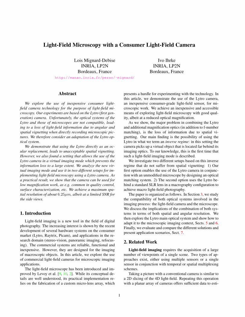
LytroCamera

SecondLens

FirstLens

Microscope Objective

Object: Resolution

Target

Photographs of specimens

Figure 1. Left: Microscope setup with the Lytro camera on top of two additional SLR lenses. Images of several samples have been takenunder different illumination conditions. Magnification is 3.0. Top and bottom left: brushed steel from scissors blade with lighting from theright and bottom. Top middle left: Scratched surface of a piece of metal. Bottom middle left: Plastic surface with highly retro-reflectiveproperties. The material is made of micro bubbles of transparent plastic that are invisible to the naked eye. Top middle right: Fabric witha hexagonal structure. The lighting is coming from the side and casts shadows and strong highlights on the three-dimensional structureof the fabric. Bottom middle right: Highly retro-reflective material from security reflective tape. Top right: Tonsil tissue with bright fieldillumination. Bottom right: Pins of a electronic component on a circuit board.

mate the light-field function. Calibration, synchronization,as well as the available bandwidth of the camera hardwareare the major determining features of this approach. Moredetails can be found, e.g., in [25, 23]. The strongest lim-itation of this approach for microscopic applications is thelarge size of the corresponding setups.

An alternative method for light-field capture is to multi-plex the different views onto a single sensor.

Temporal multiplexing is based on taking several picturesover time after moving the camera around static scenes. Themovements can be a translation or rotation of the camera.Alternatively, mirrors [5, 19] can be moved to generate ad-ditional virtual viewpoints. Another alternative implemen-tation are dynamic apertures [11].

Spatial multiplexing allows to record dynamic scenes.Parallax barriers and integral imaging [12] are historicallythe first approaches to spatially multiplex the acquisitionof a light-field, trading spatial resolution for angular reso-lution. A modern elaboration of this approach where thesensor and a micro-lens array are combined to form an in-camera light-field imaging system is the Hand-Held Plenop-tic Camera [17]. Alternatively, sensor masks [22, 21] or alight pipe [15] can be arranged such that in-camera light-fields can be recorded. Other methods use external arraysof mirrors instead of lenses [7], or external lens arrays [4].

Microscopy is a vast subject and many different illumi-nation and observation schemes have been developed in the

past. A general overview is given in [16]; a comprehen-sive review of microscopy techniques, including light-fieldmicroscopy, for the neuro-sciences can be found in [24].Light-field microscopy was introduced by Levoy et al. [9]and later augmented with light-field illumination [10]. Re-cently, addressing the large spatial resolution loss implicitin LFM, the group has shown that computational super-resolution can be achieved outside the focal plane of themicroscope [2, 3]. Another super-resolution scheme is com-bining a Shack-Hartmann wavefront sensor and a standard2D image to compute a high-resolution microscopic light-field [14]. LFM has been applied to polarization studies ofmineral samples [18] and initial studies for extracting depthmaps from the light-field data have been performed in mi-croscopic contexts [8, 20]. Most of the work today uses thesame optical configuration that was introduced in the origi-nal implementation [9]. With this article, we aim at provid-ing an inexpensive means of experimenting with LFM.

3. Background & Problem Statement

3.1. Light-field Microscopy

The main function of an optical microscope is to mag-nify small objects so that they can be observed with thenaked eye or a camera sensor. Light-field capabilities suchas changing the viewpoint, focusing after taking the pic-ture, and achieving 3D reconstruction of microscopic sam-

ples rely on the number of view points that can be measuredfrom a scene. This number is directly linked to the object-side numerical aperture NAo of the imaging system that isused as an image-forming system in front of the micro-lensarray of the light-field sensor and the micro-lens f-number.The object-side numerical aperture is defined as

NAo = n sin(α), (1)

where n is the index of the material in object space (usu-ally air, i.e. n = 1). The numerical aperture quantifies theextent of the cone of rays originating at an object point andbeing permitted into the optical system (see Fig. 2). Mi-croscope objectives usually have a high NAo, because it isdirectly linked to better optical resolution and a shallowerdepth of field. A high NAo is also important for light-fieldmicroscopy as the base-line of the light-field views is di-rectly linked to it.

Details on how to design a light-field microscope can befound in [9]. The most important aspect is that the f-numberof the micro-lens array matches the f-number of the micro-scope objective. The f-number F of any optical system isdefined as the ratio of its focal length f over the diameter Dof its entrance pupil (see Fig.2)

F =f

D. (2)

For a microscope of magnificationMmicroscope and numer-ical aperture NAo, a more appropriate equation taking thefinite image distance into account can be derived [1] fromEq. 2:

Fmicroscope =Mmicroscope

2NAo. (3)

The majority of microscope objectives has an f-number be-tween 15 and 40. In our experiments, we use a 10× objec-tive with an f-number of F = 20.

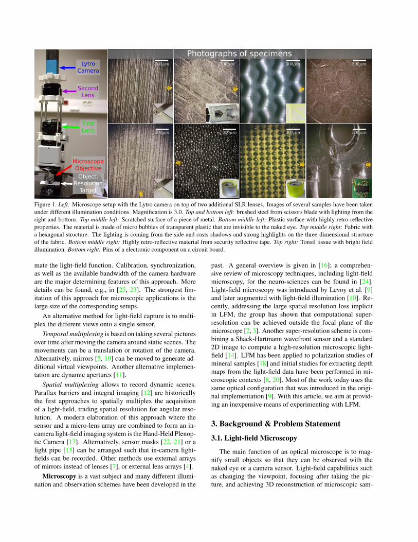
Figure 2. Properties of an optical system. An optical system isdefined by its focal length f , its principal planes H and H ′, andthe diameter D of its entrance pupil. Two conjugate planes definea unique magnification M , the ratio of the image size y′ over theobject size y. All optical equations can be found in [1].

3.2. Lytro Features

The Lytro camera is made of an optical system that isforming an image in the plane of a micro-lens array thatis, in turn, redirecting the light rays to a sensor. It hasa 3280 × 3280 pixel CMOS sensor with 12-bit A/D and

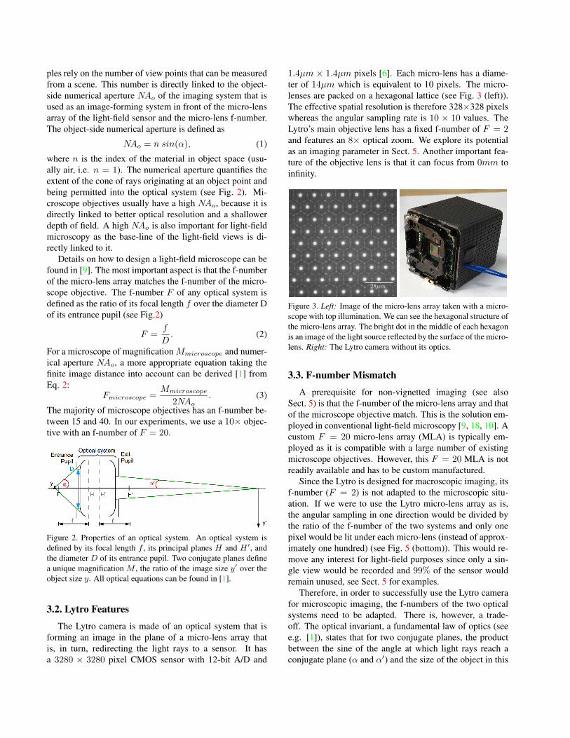
1.4µm × 1.4µm pixels [6]. Each micro-lens has a diame-ter of 14µm which is equivalent to 10 pixels. The micro-lenses are packed on a hexagonal lattice (see Fig. 3 (left)).The effective spatial resolution is therefore 328×328 pixelswhereas the angular sampling rate is 10 × 10 values. TheLytro’s main objective lens has a fixed f-number of F = 2and features an 8× optical zoom. We explore its potentialas an imaging parameter in Sect. 5. Another important fea-ture of the objective lens is that it can focus from 0mm toinfinity.

Figure 3. Left: Image of the micro-lens array taken with a micro-scope with top illumination. We can see the hexagonal structure ofthe micro-lens array. The bright dot in the middle of each hexagonis an image of the light source reflected by the surface of the micro-lens. Right: The Lytro camera without its optics.

3.3. F-number Mismatch

A prerequisite for non-vignetted imaging (see alsoSect. 5) is that the f-number of the micro-lens array and thatof the microscope objective match. This is the solution em-ployed in conventional light-field microscopy [9, 18, 10]. Acustom F = 20 micro-lens array (MLA) is typically em-ployed as it is compatible with a large number of existingmicroscope objectives. However, this F = 20 MLA is notreadily available and has to be custom manufactured.

Since the Lytro is designed for macroscopic imaging, itsf-number (F = 2) is not adapted to the microscopic situ-ation. If we were to use the Lytro micro-lens array as is,the angular sampling in one direction would be divided bythe ratio of the f-number of the two systems and only onepixel would be lit under each micro-lens (instead of approx-imately one hundred) (see Fig. 5 (bottom)). This would re-move any interest for light-field purposes since only a sin-gle view would be recorded and 99% of the sensor wouldremain unused, see Sect. 5 for examples.

Therefore, in order to successfully use the Lytro camerafor microscopic imaging, the f-numbers of the two opticalsystems need to be adapted. There is, however, a trade-off. The optical invariant, a fundamental law of optics (seee.g. [1]), states that for two conjugate planes, the productbetween the sine of the angle at which light rays reach aconjugate plane (α and α′) and the size of the object in this

plane (y and y′) is equal at both planes.

y n sin(α) = y′ n′ sin(α′), (4)

n and n′ are the optical index of the media on both sides ofthe optical system. For air, the index is equal to 1.

We therefore opt for an optical demagnification scheme,decreasing y′, to increase the angular size of the cone oflight rays α′ that is incident on the Lytro’s light-field sensor.Theoretically, we need to divide the microscope objective’sf-number by 10 to reach the same f-number as the Lytrocamera. An immediate consequence from Eq. 3 is that thecombination of all optical elements must therefore have amagnification divided by 10, i.e. we are aiming to convertthe system to unit-magnification. Due to the small size ofthe Lytro’s micro-lenses, the optical resolution of the sys-tem is still satisfactory, even at this low magnification (seeSect. 7).

The magnification of the combined system Mfinal canbe written as the product of the magnifications of each indi-vidual system:

Mfinal =MmicroscopeMlens1 ... MlensNMLytro, (5)

where Mlensi, i=1..N indicates the magnification of Nto-be-designed intermediate lens systems. The microscopeobjective has a fixed magnification of Mmicroscope = 10,whereas the lowest magnification setting of the Lytro has avalue of MLytro = 0.5. The resulting Mfinal = 5 with-out additional optical components (N = 0) is too large toprevent angular information loss.

We explore two different options (see Fig. 4) to imple-ment the adapted system. The first option (see Sect. 5) isto demagnify the image of the microscope with additionallenses (N = 2). This solution lets us use the microscopeand the Lytro camera unmodified. The second option isto remove the microscope, replacing it by an SLR lens inmacro-imaging mode. Here, we compare a setup with andwithout the Lytro optics (see Sect. 6).

Figure 4. The diagram shows our two proposed solutions toachieve low magnification. The first option (first row) keeps thecamera and the microscope intact. The second option (second row)replaces the microscope with an SLR lens.

4. Sensor CoverageVignetting: When using two or more optical systems inconjunction, some light rays are lost because the pupils ofthe different systems do not match each other. This effectis called vignetting. Generally, there are two types of vi-gnetting: spatial and angular vignetting.

Spatial vignetting directly translates into a loss of fieldof view, which may reduce the image size at the sensor (seeFig. 5 (top)). Angular vignetting (see Fig. 5 (bottom)) oc-curs when the cone of rays permitted through one of thesystems is smaller than for the other system, e.g. due to astop positioned inside the system. Angular vignetting is notan issue in a standard camera : it only affects the exposureand is directly linked to the depth of field of the camera. Ina light-field camera, however, it is crucial to minimize an-gular vignetting in order to prevent the loss of directionallight-field information.

Figure 5. Top: Spatial vignetting occurs when light rays from theobject (in red) do not pass through the second lens. For non-vignetted imaging, light rays (in blue) converging to a point at thesensor edge should include all the red light rays emerging fromthe object. Bottom: Representation of the sampling of a cone oflight rays by a F = 2 micro-lens. Green rays symbolize the an-gular cone that can be acquired by the micro-lens, while blue raysemerge from an F = 20 optical system. As can be seen from thefigure, angular vignetting prevents an effective sensor utilization.

We propose to measure the vignetting in terms of itsadaptation to the recording light-field sensor. An ideal opti-cal system that is adapted to a particular sensor would fullycover all its sensor elements. Since the raw pixel resolutionis divided into spatial and angular parts, the sensor coveragecsensor can be approximately expressed as

csensor[%] = cspatial[%]× cangular[%], (6)

where cspatial is the spatial coverage of the sensor in per-cent, and cangular is the angular coverage of one micro-lenssub-image, also in percent. In our experimental validation,we measure the spatial coverage in the center view and the

angular coverage in the center lenslet. This choice is moti-vated by the simpler estimation of the relevant coverage ar-eas as compared to using the side views/edges of the field.The measure can be considered to be an approximation ofthe upper bound of the system space-bandwidth product, i.e.the optical information capacity of the system [13].

4.1. Unmodified Use of the Lytro’s Main Optics

The main optics of the Lytro camera, i.e. the opticswithout the micro-lens array, is designed to avoid angularvignetting when imaging onto the micro-lens array, i.e. themicro-lens array and the main optics have been designedwith the same f-number of F = 2. We have observedthat the main optical system can be used in two differentways with a microscope. These two imaging regimes canbe used differently in designing an optical matching system.

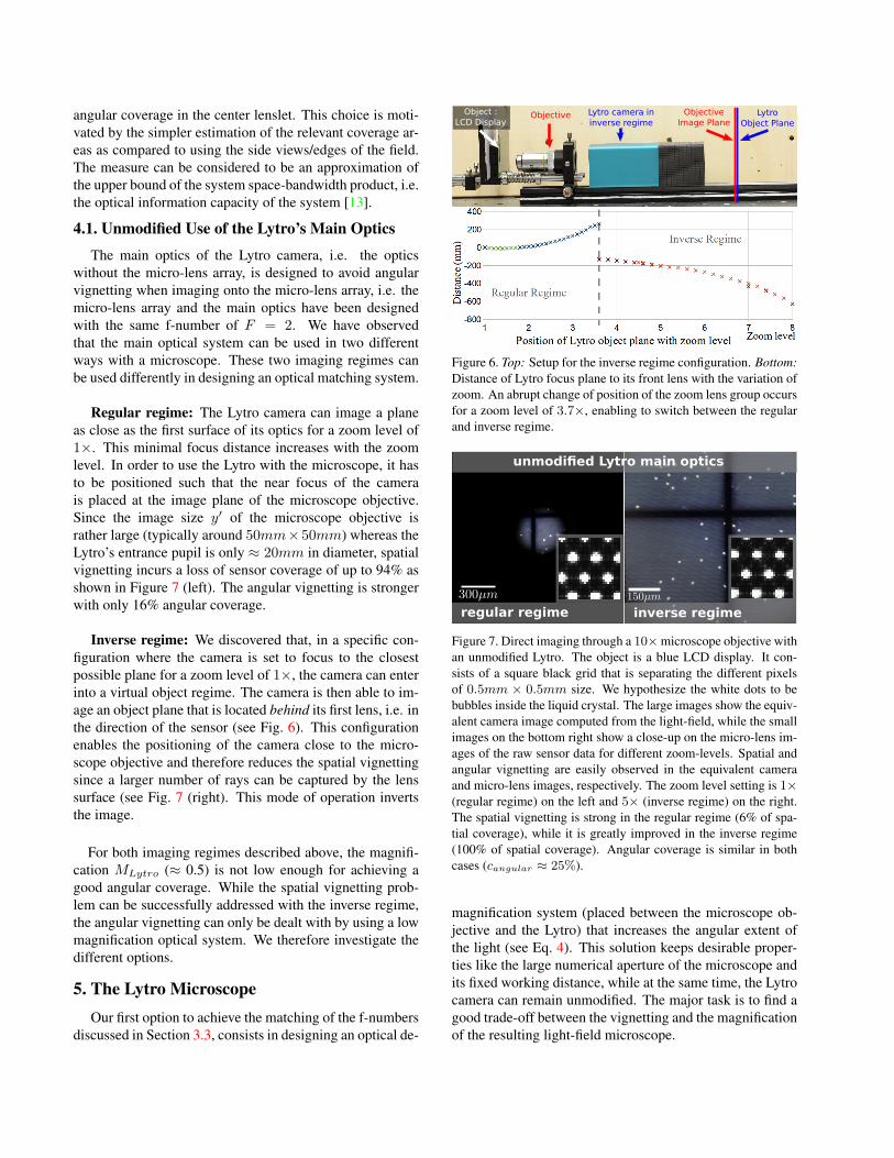
Regular regime: The Lytro camera can image a planeas close as the first surface of its optics for a zoom level of1×. This minimal focus distance increases with the zoomlevel. In order to use the Lytro with the microscope, it hasto be positioned such that the near focus of the camerais placed at the image plane of the microscope objective.Since the image size y′ of the microscope objective israther large (typically around 50mm×50mm) whereas theLytro’s entrance pupil is only ≈ 20mm in diameter, spatialvignetting incurs a loss of sensor coverage of up to 94% asshown in Figure 7 (left). The angular vignetting is strongerwith only 16% angular coverage.

Inverse regime: We discovered that, in a specific con-figuration where the camera is set to focus to the closestpossible plane for a zoom level of 1×, the camera can enterinto a virtual object regime. The camera is then able to im-age an object plane that is located behind its first lens, i.e. inthe direction of the sensor (see Fig. 6). This configurationenables the positioning of the camera close to the micro-scope objective and therefore reduces the spatial vignettingsince a larger number of rays can be captured by the lenssurface (see Fig. 7 (right). This mode of operation invertsthe image.

For both imaging regimes described above, the magnifi-cation MLytro (≈ 0.5) is not low enough for achieving agood angular coverage. While the spatial vignetting prob-lem can be successfully addressed with the inverse regime,the angular vignetting can only be dealt with by using a lowmagnification optical system. We therefore investigate thedifferent options.

5. The Lytro MicroscopeOur first option to achieve the matching of the f-numbers

discussed in Section 3.3, consists in designing an optical de-

Objective Lytro camera in inverse regime

Objective Image Plane

Lytro Object Plane

Object : LCD Display

Figure 6. Top: Setup for the inverse regime configuration. Bottom:Distance of Lytro focus plane to its front lens with the variation ofzoom. An abrupt change of position of the zoom lens group occursfor a zoom level of 3.7×, enabling to switch between the regularand inverse regime.

inverse regimeregular regime

unmodified Lytro main optics

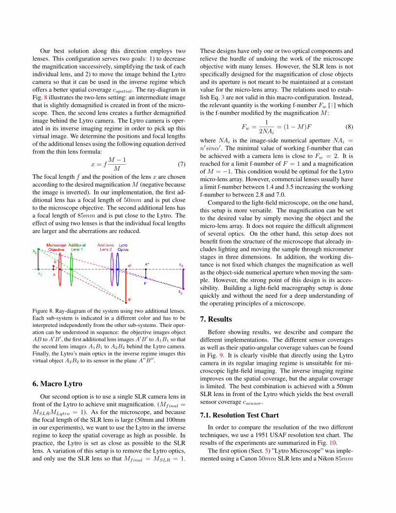
Figure 7. Direct imaging through a 10× microscope objective withan unmodified Lytro. The object is a blue LCD display. It con-sists of a square black grid that is separating the different pixelsof 0.5mm × 0.5mm size. We hypothesize the white dots to bebubbles inside the liquid crystal. The large images show the equiv-alent camera image computed from the light-field, while the smallimages on the bottom right show a close-up on the micro-lens im-ages of the raw sensor data for different zoom-levels. Spatial andangular vignetting are easily observed in the equivalent cameraand micro-lens images, respectively. The zoom level setting is 1×(regular regime) on the left and 5× (inverse regime) on the right.The spatial vignetting is strong in the regular regime (6% of spa-tial coverage), while it is greatly improved in the inverse regime(100% of spatial coverage). Angular coverage is similar in bothcases (cangular ≈ 25%).

magnification system (placed between the microscope ob-jective and the Lytro) that increases the angular extent ofthe light (see Eq. 4). This solution keeps desirable proper-ties like the large numerical aperture of the microscope andits fixed working distance, while at the same time, the Lytrocamera can remain unmodified. The major task is to find agood trade-off between the vignetting and the magnificationof the resulting light-field microscope.

Our best solution along this direction employs twolenses. This configuration serves two goals: 1) to decreasethe magnification successively, simplifying the task of eachindividual lens, and 2) to move the image behind the Lytrocamera so that it can be used in the inverse regime whichoffers a better spatial coverage cspatial. The ray-diagram inFig. 8 illustrates the two-lens setting: an intermediate imagethat is slightly demagnified is created in front of the micro-scope. Then, the second lens creates a further demagnifiedimage behind the Lytro camera. The Lytro camera is oper-ated in its inverse imaging regime in order to pick up thisvirtual image. We determine the positions and focal lengthsof the additional lenses using the following equation derivedfrom the thin lens formula:

x = fM − 1

M(7)

The focal length f and the position of the lens x are chosenaccording to the desired magnificationM (negative becausethe image is inverted). In our implementation, the first ad-ditional lens has a focal length of 50mm and is put closeto the microscope objective. The second additional lens hasa focal length of 85mm and is put close to the Lytro. Theeffect of using two lenses is that the individual focal lengthsare larger and the aberrations are reduced.

Figure 8. Ray-diagram of the system using two additional lenses.Each sub-system is indicated in a different color and has to beinterpreted independently from the other sub-systems. Their oper-ation can be understood in sequence: the objective images objectAB to A′B′, the first additional lens images A′B′ to A1B1 so thatthe second lens images A1B1 to A2B2 behind the Lytro camera.Finally, the Lytro’s main optics in the inverse regime images thisvirtual object A2B2 to its sensor in the plane A′′B′′.

6. Macro LytroOur second option is to use a single SLR camera lens in

front of the Lytro to achieve unit magnification. (Mfinal =MSLRMLytro = 1). As for the microscope, and becausethe focal length of the SLR lens is large (50mm and 100mmin our experiments), we want to use the Lytro in the inverseregime to keep the spatial coverage as high as possible. Inpractice, the Lytro is set as close as possible to the SLRlens. A variation of this setup is to remove the Lytro optics,and only use the SLR lens so that Mfinal = MSLR = 1.

These designs have only one or two optical components andrelieve the hurdle of undoing the work of the microscopeobjective with many lenses. However, the SLR lens is notspecifically designed for the magnification of close objectsand its aperture is not meant to be maintained at a constantvalue for the micro-lens array. The relations used to estab-lish Eq. 3 are not valid in this macro-configuration. Instead,the relevant quantity is the working f-number Fw [1] whichis the f-number modified by the magnification M :

Fw =1

2NAi= (1−M)F (8)

where NAi is the image-side numerical aperture NAi =n′sinα′. The minimal value of working f-number that canbe achieved with a camera lens is close to Fw = 2. It isreached for a limit f-number of F = 1 and a magnificationof M = −1. This condition would be optimal for the Lytromicro-lens array. However, commercial lenses usually havea limit f-number between 1.4 and 3.5 increasing the workingf-number to between 2.8 and 7.0.

Compared to the light-field microscope, on the one hand,this setup is more versatile. The magnification can be setto the desired value by simply moving the object and themicro-lens array. It does not require the difficult alignmentof several optics. On the other hand, this setup does notbenefit from the structure of the microscope that already in-cludes lighting and moving the sample through micrometerstages in three dimensions. In addition, the working dis-tance is not fixed which changes the magnification as wellas the object-side numerical aperture when moving the sam-ple. However, the strong point of this design is its acces-sibility. Building a light-field macrography setup is donequickly and without the need for a deep understanding ofthe operating principles of a microscope.

7. ResultsBefore showing results, we describe and compare the

different implementations. The different sensor coveragesas well as their spatio-angular coverage values can be foundin Fig. 9. It is clearly visible that directly using the Lytrocamera in its regular imaging regime is unsuitable for mi-croscopic light-field imaging. The inverse imaging regimeimproves on the spatial coverage, but the angular coverageis limited. The best combination is achieved with a 50mmSLR lens in front of the Lytro which yields the best overallsensor coverage csensor.

7.1. Resolution Test Chart

In order to compare the resolution of the two differenttechniques, we use a 1951 USAF resolution test chart. Theresults of the experiments are summarized in Fig. 10.

The first option (Sect. 5) ”Lytro Microscope” was imple-mented using a Canon 50mm SLR lens and a Nikon 85mm

Figure 9. Combined results of the experiments from Sect. 5 andSect. 6.

Figure 10. This table summarizes the results from the experimentsof Sect. 5 and Sect. 6. Theoretical resolution is derived from themicro-lens pitch. The micro-lens footprint is the size of a micro-lens in object space.

SLR lens as additional lenses. Those lenses were put ontop of a Leitz Ergolux microscope using an objective ofmagnification 10× with an object-side numerical apertureNAo = 0.2. This microscope has a lens tube with a mag-nification of 0.8× so the f-number F = 20. The imageshave been taken with a magnification of 2.88, i.e. a micro-lens covers 4.87µm in object space (see Fig. 11 (top)). Thespatial coverage is above 99% but due to the large magnifi-cation the angular coverage is low (between 9% and 25%).The resolution is between 80 and 90 line pairs per mm.

The resolution indicated above is computed for the cen-ter view. It decreases with further distance from the center.A loss of image quality due to aberrations can be observed.They are introduced because the observed area is largerthan usual for the microscope objective. Microscope ob-jectives are typically designed so that only a reduced innerportion of the full field is very well corrected. In addition,our matching lenses introduce further aberrations. Since theangular vignetting is strong, the contrast of viewpoints farfrom the center is low. It should be noted that even view-points inside the vignetted area can be computed, albeit at apoor signal-to-noise ratio (see Fig. 11).

The second option (Sect. 6) was implemented in threeways: two times with the Lytro placed behind two differentlenses, a 50mm and a 100mm Canon SLR lens (referred asSLR + Lytro), and with the Lytro micro-lens array withoutthe Lytro main optics, see Fig. 3 (right), placed behind the50mm lens (referred as SLR + MLA) (see Fig. 12). Magni-fications from 1.26 to 2.34 were achieved. The spatial cov-erage is always 100% and angular coverage is good (up to70%). In this case, chromatic aberrations are present which

degrades the image. The aberrations are reduced in the SLR+ Lytro case as compared to SLR + MLA, since the magni-fication of the SLR lens is lower in this setting. It is mostnoticable in the side views since, for these views, imaging isperformed through the outer pupil regions of the SLR lens.We suspect that the chromatic aberration is introduced bythe SLR lens because it is not intended for macro-imaging.Using a dedicated macro-lens instead would likely removethis effect.

Object: Resolution

target

SLR Lens 100mm

Lytro Camera

Figure 12. Setup from the SLR + Lytro experiment using a 100mmSLR lens (100mm SLR + Lytro).

7.2. Microscopic Sample

The most direct application of the light-field microscopeis the study of microscopic samples. The low magnificationand the large field of view allow us to see in detail an objectarea that is between 1.5mm×1.5mm and 3.5mm×3.5mmwith a magnification of 2.88× and 1.3× respectively. Celltissues or rough surfaces of different materials have a struc-ture close to the millimeter so high magnification is not al-ways necessary to analyze them.

We illustrate this technique in Fig. 1 (right). Several im-ages of microscopic specimen were taken with the same set-tings as in the previous section. The magnification is 2.88×and we can clearly see the structure of different kind of sur-faces that are invisible to the naked eye.

The light-field data allows for the reconstruction of thedepth of the sample when the number of views is suffi-cient. We took a picture of a ground truth aluminium stair-case with stairs of 1.00mm width and 0.50mm height withan accuracy of ±5µm with the 50mmSLR + Lytro setup.We obtained the depth map in Fig. 13 using a modifiedvariational multi-scale optical flow algorithm for light-fielddepth estimation [15]. Although only a small slice of thestaircase is in focus (the depth of field is 1mm), the depthcan be computed outside of this area. Essentially, out-of-focus regions are naturally considered as a different scaleby the algorithm, so, the estimation of the depth of the clos-est and furthest steps is correct. This behavior nicely inter-acts with the scene properties since the parallax is larger inout-of-focus regions. The optical system can be seen as sup-porting the part of the algorithm that is handling large dis-

Figure 11. Set of different viewpoints of the resolution target with the center view in the middle (the red dot in the top left inset indicatesthe position of the view). Top: Images taken with the ”Lytro Microscope” (Sect. 5). The magnification is 2.88. Bottom: Images taken withthe ”50mmSLR + Lytro” (Sect. 6). A red-green color shift due to strong chromatic aberrations can be observed in the side views. Note thatthe top row has a higher resolution: it shows the pattern that is visible in the center of the bottom row (level 4 and 5). The contrast of theimages of the same row have been set to a similar level for comparison.

placements. Since the detailed properties of the Lytro mainoptics are unknown, it is necessary to adjust the scale of thecomputed depth. We use the aluminium staircase as refer-ence. We find the affine transformation between the depthmap and the staircase model by fitting planes to match thestairs. After the transformation, we measure an RMS errorof 75µm for vertical planes and 17µm for horizontal planes.The difference is due to the different slopes of the horizontaland vertical steps with relation to the camera view direction.The magnification is equal to 1.32. We also applied thisdepth reconstruction to a daisy head (see Fig. 13). In prac-tice, the depth inside a cube of about 3.5 × 3.5 × 3.5mm3

can be estimated, which is rather large for a microscopicsetting.

8. Discussion and Conclusion

We have developed and tested several adaptations ofthe Lytro consumer light-field camera to enable an entry-level experimentation with light-field microscopy. Whilethe fixed f-number of the Lytro’s micro-lens array preventsits direct use with a standard microscope (regular regime),it is possible to trade the overall system magnification forlight-field features and to avoid spatial vignetting with theinverse imaging regime. Lytro microscopy is therefore anoption for low-magnification work as is common in indus-trial settings, or for investigations into the meso- and large-scale micro-structure of materials. Even though an opticalmagnification between 1 and 3, as achieved in this work, ap-pears to be low, the small size of the micro-lenses still yieldsa decent optical resolution of up to 6.25µm in object spacewhich already shows interesting optical structures that areimperceivable by the naked eye.

Figure 13. Sub-view (top left) and computed depth map (top mid-dle) of a daisy flower. Sub-view (bottom left) and computed depthmap (bottom middle) of the aluminium staircase. The bottom rightpicture is a 3D visualization of the depth map after the calibratingand the top right picture is a projection of a region in the middle ofthe calibrated depth map onto the xz plane showing the plane fitsin red.

For the future, we would like to investigate image-baseddenoising schemes for the vignetted side-views, as well asalgorithmic developments for structure recovery. In termsof applications, the imaging of micro-and meso-BRDFs andtheir relation to macroscopic BRDF models appears to be aninteresting development.

AcknowledgementsWe would also like to thank Patrick Reuter for his

helpful comments. This work was supported by theGerman Research Foundation (DFG) through Emmy-Noether fellowship IH 114/1-1 as well as the ANR

ISAR project of the French Agence Nationale de laRecherche.

References[1] M. Born and E. Wolf. Principles of optics. Pergamon Press,

1980. 3, 6[2] M. Broxton, L. Grosenick, S. Yang, N. Cohen, A. Andal-

man, K. Deisseroth, and M. Levoy. Wave Optics Theory and3-D Deconvolution for the Light Field Microscope. OpticsExpress, 21(21):25418–25439, 2013. 1, 2

[3] N. Cohen, S. Yang, A. Andalman, M. Broxton, L. Grosenick,K. Deisseroth, M. Horowitz, and M. Levoy. Enhancing theperformance of the light field microscope using wavefrontcoding. Optics express, 22(20):24817–24839, 2014. 2

[4] T. Georgiev and C. Intwala. Light field camera design forintegral view photography. Technical report, Adobe System,Inc, 2006. 2

[5] I. Ihrke, T. Stich, H. Gottschlich, M. Magnor, and H.-P. Sei-del. Fast incident light field acquisition and rendering. Jour-nal of WSCG (WSCG’08), 16(1-3):25–32, 2008. 2

[6] J. Kucera. Lytro meltdown. http://optics.miloush.net/lytro/Default.aspx, 2014. 3

[7] D. Lanman, D. Crispell, M. Wachs, and G. Taubin. Spher-ical catadioptric arrays: Construction, multi-view geometry,and calibration. In 3D Data Processing, Visualization, andTransmission, Third International Symposium on, pages 81–88. IEEE, 2006. 2

[8] J.-J. Lee, D. Shin, B.-G. Lee, and H. Yoo. 3D OpticalMicroscopy Method based on Synthetic Aperture IntegralImaging. 3D Research, 3(4):1–6, 2012. 2

[9] M. Levoy, R. Ng, A. Adams, M. Footer, and M. Horowitz.Light field microscopy. In ACM Transactions on Graphics(TOG), volume 25, pages 924–934. ACM, 2006. 1, 2, 3

[10] M. Levoy, Z. Zhang, and I. McDowall. Recording and Con-trolling the 4D Light Field in a Microscope using MicrolensArrays. Journal of Microscopy, 235:144–162, 2009. 1, 2, 3

[11] C.-K. Liang, T.-H. Lin, B.-Y. Wong, C. Liu, and H. H. Chen.Programmable aperture photography: Multiplexed light fieldacquisition. ACM Trans. on Graphics, 27(3):1–10, 2008. 2

[12] G. Lippman. Epreuves reversibles photographies integrales.CR Acad. Sci, 146:446–451, 1908. 2

[13] A. W. Lohmann, R. G. Dorsch, D. Mendlovic, Z. Zalevsky,and C. Ferreira. Space-Bandwidth Product of Optical Signalsand Systems. Journal of the Optical Society of America A,13(3):470–473, 1996. 5

[14] C.-H. Lu, S. Muenzel, and J. Fleischer. High-resolutionLight-Field Microscopy. In Computational Optical Sensingand Imaging, pages CTh3B–2. Optical Society of America,2013. 2

[15] A. Manakov, J. Restrepo, O. Klehm, R. Hegedus, H.-P. Sei-del, E. Eisemann, and I. Ihrke. A Reconfigurable CameraAdd-On for High Dynamic Range, Multispectral, Polariza-tion, and Light-Field Imaging. ACM Trans. on Graphics(SIGGRAPH’13), 32(4):article 47, 2013. 2, 7

[16] D. B. Murphy and M. W. Davidson. Fundamentals of LightMicroscopy and Electronic Imaging. John Wiley & Sons,2012. 2

[17] R. Ng, M. Levoy, M. Bredif, G. Duval, M. Horowitz,and P. Hanrahan. Light field photography with a hand-held plenoptic camera. Computer Science Technical ReportCSTR, 2(11), 2005. 2

[18] R. Oldenbourg. Polarized Light Field Microscopy: An An-alytical Method using a Microlens Array to SimultaneouslyCapture both Conoscopic and Orthoscopic Views of Bire-fringent Objects. Journal of Microscopy, 231(3):419–432,2008. 2, 3

[19] Y. Taguchi, A. Agrawal, S. Ramalingam, and A. Veeraragha-van. Axial light field for curved mirrors: Reflect your per-spective, widen your view. In Computer Vision and PatternRecognition (CVPR), 2010 IEEE Conference on, pages 499–506. IEEE, 2010. 2

[20] M. Thomas, I. Montilla, J. Marichal-Hernandez,J. Fernandez-Valdivia, J. Trujillo-Sevilla, and J. Rodriguez-Ramos. Depth Map Extraction from Light Field Micro-scopes. In 12th Workshop on Information Optics (WIO),pages 1–3. IEEE, 2013. 2

[21] A. Veeraraghavan, R. Raskar, A. Agrawal, R. Chellappa,A. Mohan, and J. Tumblin. Non-Refractive Modulators forEncoding and Capturing Scene Appearance and Depth. InIEEE Conference on Computer Vision and Pattern Recogni-tion (CVPR), pages 1–8, 2008. 2

[22] A. Veeraraghavan, R. Raskar, A. Agrawal, A. Mohan, andJ. Tumblin. Dappled Photography: Mask Enhanced Cam-eras For Heterodyned Light Fields and Coded Aperture Re-focussing. ACM Trans. on Graphics (TOG), 26:69, 2007. 2

[23] B. Wilburn, N. Joshi, V. Vaish, E.-V. Talvala, E. Antunez,A. Barth, A. Adams, M. Horowitz, and M. Levoy. Highperformance imaging using large camera arrays. In ACMTrans. on Graphics (TOG), volume 24, pages 765–776.ACM, 2005. 2

[24] B. A. Wilt, L. D. Burns, E. T. W. Ho, K. K. Ghosh, E. A.Mukamel, and M. J. Schnitzer. Advances in Light Mi-croscopy for Neuroscience. Annual Review of Neuroscience,32:435, 2009. 2

[25] J. C. Yang, M. Everett, C. Buehler, and L. McMillan. Areal-time distributed light field camera. In Proceedings ofthe 13th Eurographics workshop on Rendering, pages 77–86. Eurographics Association, 2002. 2