Embed Size (px)
Citation preview
Noname manuscript No.
(will be inserted by the editor)
Light-time computations for the BepiColombo Radio
Science Experiment
G. Tommei · A. Milani · D. Vokrouhlicky
Received: date / Accepted: date
Abstract The Radio Science Experiment is one of the on board experiments of the
Mercury ESA mission BepiColombo that will be launched in 2014. The goals of the
experiment are to determine the gravity field of Mercury and its rotation state, to deter-
mine the orbit of Mercury, to constrain the possible theories of gravitation (for example
by determining the post-Newtonian (PN) parameters), to provide the spacecraft posi-
tion for geodesy experiments and to contribute to planetary ephemerides improvement.
This is possible thanks to a new technology which allows to reach great accuracies in
the observables range and range rate; it is well known that a similar level of accuracy
requires studying a suitable model taking into account numerous relativistic effects.
In this paper we deal with the modelling of the space-time coordinate transformations
needed for the light-time computations and the numerical methods adopted to avoid
rounding-off errors in such computations.
Keywords Mercury · Interplanetary tracking · Light-time · Relativistic effects ·
Numerical methods
1 Introduction
BepiColombo is an European Space Agency mission to be launched in 2014, with the
goal of an in-depth exploration of the planet Mercury; it has been identified as one
of the most challenging long-term planetary projects. Only two NASA missions had
Mercury as target in the past, the Mariner 10, which flew by three times in 1974-5 and
G. Tommei, A. MilaniDepartment of Mathematics, University of Pisa, Largo B. Pontecorvo 5, 56127 Pisa, ItalyE-mail: [email protected]
A. MilaniE-mail: [email protected]
D. VokrouhlickyInstitute of Astronomy, Charles University, V Holesovickach 2, CZ-18000 Prague 8, CzechRepublicE-mail: [email protected]
2
Messenger, which carried out its flybys on January and October 2008, September 2009
before it starts its year-long orbiter phase in March 2011.
The BepiColombo mission is composed by two spacecraft to be put in orbit around
Mercury. The Radio Science Experiment is one of the on board experiments, which
would coordinate a gravimetry, a rotation and a relativity experiment, using a very
accurate range and range rate tracking. These measurements will be performed by a
full 5-way link to the Mercury orbiter; by exploiting the frequency dependence of the
refraction index, the differences between the Doppler measurements (done in Ka and X
band) and the delay give information on the plasma content along the radio wave path
(Iess and Boscagli 2001). In this way most of the measurements errors introduced can
be reduced by about two orders of magnitude with respect to the past technologies.
The accuracies that can be achieved are 10 cm in range and 3 × 10⁻⁴ cm/s in range
rate.
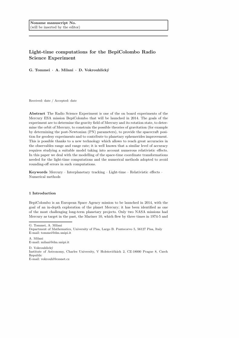
How do we compute these observables? For example, a first approximation of the
range could be given by the formula
r = |r| = |(xsat + xM) − (xEM + xE + xant)| , (1)
which models a very simple geometrical situation (Figure 1). The vector xsat is the
mercurycentric position of the orbiter, the vector xM is the position of the center of
mass of Mercury (M) in a reference system with origin at the Solar System Barycenter
(SSB), the vector xEM is the position of the Earth-Moon center of mass in the same
reference system, xE is the vector from the Earth-Moon Barycenter (EMB) to the
center of mass of the Earth (E), the vector xant is the position of the reference point
of the ground antenna with respect to the center of mass of the Earth.
r
xM x
xant
xE
xsat
EM
SSB
M ant
sat
EMB
E
Fig. 1 Geometric sketch of the vectors involved in the computation of the range. SSB is theSolar System Barycenter, M is the center of Mercury, EMB is the Earth-Moon Barycenter, Eis the center of the Earth.
Using (1) means to model the space as a flat arena (r is an Euclidean distance)
and the time as an absolute parameter. This is obviously not possible because it is
clear that, beyond some threshold of accuracy, space and time have to be formulated
within the framework of Einstein’s theory of gravity (general relativity theory, GRT).
Moreover we have to take into account the different times at which the events have
to be computed: the transmission of the signal at the transmit time (tt), the signal at

3
the Mercury orbiter at the time of bounce (tb) and the reception of the signal at the
receive time (tr).
Formula (1) is used as a starting point to construct a correct relativistic formulation;
with the word “correct” we do not mean all the possible relativistic effects, but the
effects that can be measured by the experiment. This paper deals with the corrections
to apply to this formula to obtain a consistent relativistic model for the computations
of the observables and the practical implementation of such computations.
In Section 2 we discuss the relativistic four-dimensional reference systems used
and the transformations adopted to make the sums in (1) consistent; according to
(Soffel et al. 2003), with “reference system” we mean a purely mathematical construc-
tion, while a “reference frame” is a some physical realization of a reference system.
The relativistic contribution to the time delay due to the Sun’s gravitational field, the
Shapiro effect, is described in Section 3. Section 4 deals with the theoretical procedure
to compute the light-time (range) and the Doppler shift (range rate). In Section 5
we discuss the practical implementation of the algorithms showing how we solve the
rounding-off problems.
The equations of motion for the planets Mercury and Earth, including all the rela-
tivistic effects (and potential violations of GRT) required to the accuracy of the Bepi-
Colombo Radio Science Experiment have already been discussed in (Milani et al. 2010),
thus this paper focuses on the computation of the observables.
2 Space-time reference frames and transformations
The five vectors involved in formula (1) have to be computed at their own time, the
epoch of different events: e.g., xant, xEM and xE are computed at both the antenna
transmit time tt and receive time tr of the signal. xM and xsat are computed at the
bounce time tb (when the signal has arrived to the orbiter and is sent back, with correc-
tion for the delay of the transponder). In order to be able to perform the vector sums
and differences, these vectors have to be converted to a common space-time reference
system, the only possible choice being some realization of the BCRS (Barycentric Ce-
lestial Reference System). We adopt for now a realization of the BCRS that we call
SSB (Solar System Barycentric) reference frame and in which the time is a re-definition
of the TDB (Barycentric Dynamic Time), according to the IAU 2006 Resolution B31;
other possible choices, such as TCB (Barycentric Coordinate Time), only can differ
by linear scaling. The TDB choice of the SSB time scale entails also the appropriate
linear scaling of space-coordinates and planetary masses as described for instance in
(Klioner 2008) or (Klioner et al. 2010).
The vectors xM, xE, and xEM are already in SSB as provided by numerical integra-
tion and external ephemerides; thus the vectors xant and xsat have to be converted to
SSB from the geocentric and mercurycentric systems, respectively. Of course the con-
version of reference system implies also the conversion of the time coordinate. There are
three different time coordinates to be considered. The currently published planetary
ephemerides are provided in TDB. The observations are based on averages of clock
and frequency measurements on the Earth surface: this defines another time coordi-
nate called TT (Terrestrial Time). Thus for each observation the times of transmission
tt and reception tr need to be converted from TT to TDB to find the corresponding
1 See the Resolution at http://www.iau.org/administration/resolutions/ga2006/

4
positions of the planets, e.g., the Earth and the Moon, by combining information from
the pre-computed ephemerides and the output of the numerical integration for Mer-
cury and for the Earth-Moon barycenter. This time conversion step is necessary for the
accurate processing of each set of interplanetary tracking data; the main term in the
difference TT-TDB is periodic, with period 1 year and amplitude ≃ 1.6×10⁻³ s, while
there is essentially no linear trend, as a result of a suitable definition of the TDB.
The equation of motion of a mercurycentric orbiter can be approximated, to the
required level of accuracy, by a Newtonian equation provided the independent variable
is the proper time of Mercury. Thus, for the BepiColombo Radio Science Experiment,
it is necessary to define a new time coordinate TDM (Mercury Dynamic Time), as
described in (Milani et al. 2010), containing terms of 1-PN order depending mostly
upon the distance from the Sun and velocity of Mercury.
From now on, in accordance with (Klioner et al. 2010), we shall call the quantities
related to the SSB frame “TDB-compatible”, the quantities related to the geocentric
frame “TT-compatible”, the quantities related to the mercurycentric frame “TDM-
compatible” and label them TB, TT and TM, respectively.
The differential equation giving the local time T as a function of the SSB time t ,
which we are currently assuming to be TDB, is the following:
dT
dt= 1 −
1
c2
[
U +v2
2− L
]
, (2)
where U is the gravitational potential (the list of contributing bodies depends upon
the accuracy required: in our implementation we use Sun, Mercury to Neptune, Moon)
at the planet center and v is the SSB velocity of the same planet. The constant term
L is used to perform the conventional rescaling motivated by removal of secular terms,
e.g., for the Earth we use LC (Soffel et al. 2003).
The space-time transformations to perform involve essentially the position of the
antenna and the position of the orbiter. The geocentric coordinates of the antenna
should be transformed into TDB-compatible coordinates; the transformation is ex-
pressed by the formula
xTBant = x
TTant
(
1 −U
c2− LC
)
−1
2
(
vTBE · xTT
ant
c2
)
vTBE ,
where U is the gravitational potential at the geocenter (excluding the Earth mass),
LC = 1.48082686741 × 10⁻⁸ is a scaling factor given as definition, supposed to be
a good approximation for removing secular terms from the transformation and vTBE
is the barycentric velocity of the Earth. The next formula contains the effect on the
velocities of the time coordinate change, which should be consistently used together
with the coordinate change:
vTBant =
[
vTTant
(
1 −U
c2− LC
)
−1
2
(
vTBE · vTT
ant
c2
)
vTBE
]
[
dT
dt
]
.
Note that the previous formula contains the factor dT/dt (expressed by (2)) that deals
with a time transformation: T is the local time for Earth, that is TT, and t is the
corresponding TDB time.
5
The mercurycentric coordinates of the orbiter have to be transformed into TDB-
compatible coordinates through the formula
xTBsat = x
TMsat
(
1 −U
c2− LCM
)
−1
2
(
vTBM · xTM
sat
c2
)
vTBM ,
where U is the gravitational potential at the center of mass of Mercury (excluding
the Mercury mass) and LCM could be used to remove the secular term in the time
transformation (thus defining a TM scale, implying a rescaling of the mass of Mercury).
We believe this is not necessary: the secular drift of TDM with respect to other time
scales is significant, see Figure 5 in (Milani et al. 2010), but a simple iterative scheme
is very efficient in providing the inverse time transformation. Thus we set LCM =
0, assuming the reference frame is TDM-compatible. As for the antenna we have a
formula expressing the velocity transformation that contains the derivative of time T
for Mercury, that is TDM, with respect to time t, that is TDB:
vTBsat =
[
vTMsat
(
1 −U
c2− LCM
)
−1
2
(
vTBM · vTM
sat
c2
)
vTBM
]
[
dT
dt
]
.
For these coordinate changes, in every formula we neglected the terms of the SSB
acceleration of the planet center (Damour et al. 1994), because they contain beside
1/c2 the additional small parameter (distance from planet center)/(planet distance to
the Sun), which is of the order of 10−4 even for a Mercury orbiter.
To assess the relevance of the relativistic corrections of this section to the accuracy
of the BepiColombo Radio Science Experiment, we computed the observables range and
range rate with and without these corrections. As shown in Figure 2, the differences
are significant, at a signal-to-noise ratio S/N ≃ 1 for range, much more for range rate,
with an especially strong signature from the orbital velocity of the mercurycentric orbit
(with S/N > 50).
3 Shapiro effect
The correct modelling of space-time transformations is not sufficient to have a precise
computation of the signal delay: we have to take into account the general relativistic
contribution to the time delay due to the space-time curvature under the effect of the
Sun’s gravitational field, the Shapiro effect (Shapiro 1964). The Shapiro time delay ∆t
at the 1-PN level, according to (Will 1993) and (Moyer 2003), is
∆t =(1 + γ)µ0
c3ln(
rt + rr + r
rt + rr − r
)
, S(γ) = c ∆t
where rt = |rt| and rr = |rr| are the heliocentric distances of the transmitter and the
receiver at the corresponding time instants of photon transmission and reception, µ0 is
the gravitational mass of the Sun (µ0 = G m0) and r = |rr − rt|. The planetary terms,
similar to the solar one, can also be included but they are smaller than the accuracy
needed for our measurements. Parameter γ is the only post-Newtonian parameter used
for the light-time effect and, in fact, it could be best constrained during superior con-
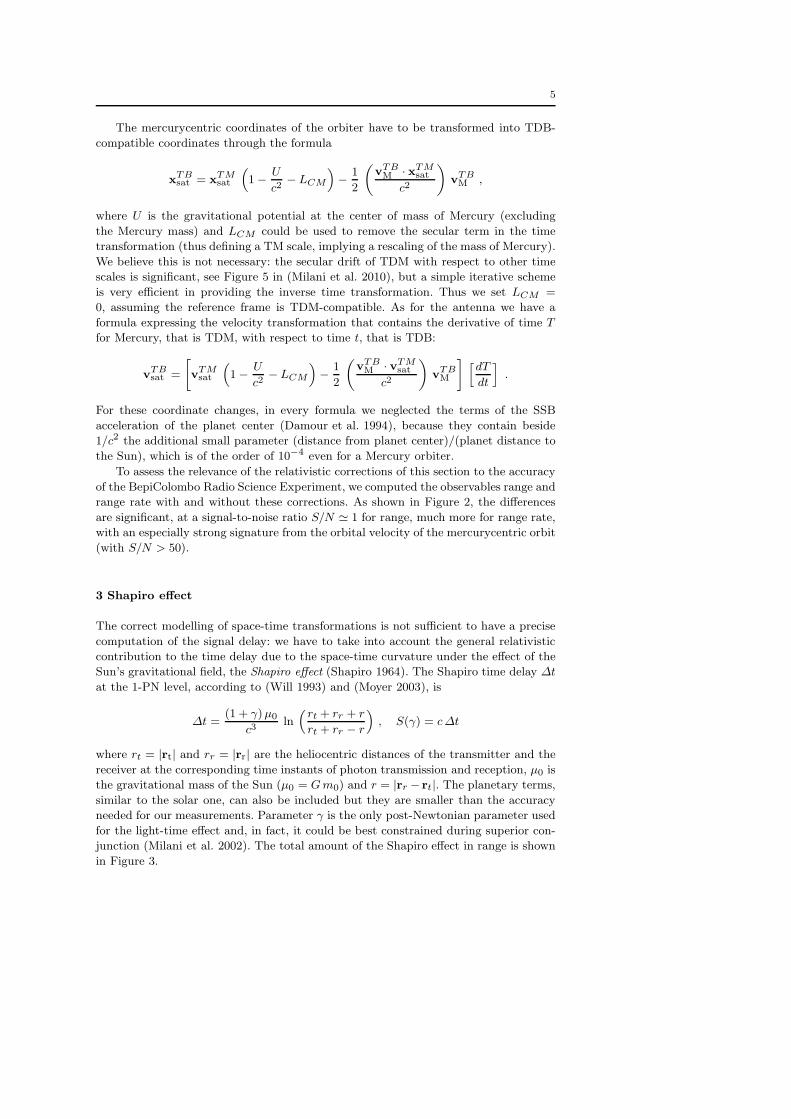
junction (Milani et al. 2002). The total amount of the Shapiro effect in range is shown
in Figure 3.

6
0 0.05 0.1 0.15 0.2 0.25 0.3 0.35 0.4 0.45−10
−5
0
5Change in the observable
time, days from arc beginning
Ran
ge, c
m
0 0.05 0.1 0.15 0.2 0.25 0.3 0.35 0.4 0.45−0.02
−0.01
0
0.01
0.02
time, days from arc beginning
Ran
ge−
rate
, cm
/s
0 0.05 0.1 0.15 0.2 0.25 0.3 0.35 0.4 0.45−16
−14
−12
−10
−8
−6
−4Change in the observable
time, days from arc beginning
Ran
ge, c
m
0 0.05 0.1 0.15 0.2 0.25 0.3 0.35 0.4 0.45−1.5
−1
−0.5
0
0.5
1
1.5
2x 10
−3
time, days from arc beginning
Ran
ge−
rate
, cm
/s
Fig. 2 The difference in the observables range and range rate for one pass of Mercury abovethe horizon for a ground station, by using an hybrid model in which the position and velocity ofthe orbiter have not transformed to TDB-compatible quantities and a correct model in whichall quantities are TDB-compatible. Interruptions of the signal are due to spacecraft passagebehind Mercury as seen for the Earth station. Top: for an hybrid model with the satelliteposition and velocity not transformed to TDB-compatible. Bottom: for an hybrid model withthe position and velocity of the antenna not transformed to TDB-compatible.
The question arises whether the very high signal to noise in the range requires
other terms in the solar gravity influence, due to either (i) motion of the source, or
(ii) higher-order corrections when the radio waves are passing near the Sun, at just a
few solar radii (and thus the denominator in the log-function of the Shapiro formula
is small). The corrections (i) are of the post-Newtonian order 1.5 (containing a factor
1/c3), but it has been shown in (Milani et al. 2010) that they are too small to affect
our accuracy. The corrections (ii) are of order 2, (containing a factor 1/c4), but they
can be actually larger for an experiment involving Mercury. The relevant correction is
most easily obtained by adding 1/c4 terms in the Shapiro formula, due to the bending
of the light path:
S(γ) =(1 + γ)µ0
c2ln
(
rt + rr + r +(1+γ) µ0
c2
rt + rr − r +(1+γ) µ0
c2
)
.
This formulation has been proposed by (Moyer 2003) and it has been justified
in the small impact parameter regime by much more theoretically rooted deriva-
7
0 100 200 300 400 500 600 700 8000
0.5
1
1.5
2
2.5x 10
6 Change in the observable
time, days from arc beginning
Ran
ge, c
m
Fig. 3 Total amount of the Shapiro effect in range over 2-year simulation. The sharp peakscorrespond to superior conjunctions, when Mercury is “behind the Sun” as seen from Earth,with values as large as 24 km for radio waves passing at 3 solar radii from the center of theSun. Interruptions of the signal are due to spacecraft visibility from the Earth station (in thissimulation we assume just one station).
tions by (Klioner and Zschocke 2007), (Teyssandier and Le Poncin-Lafitte 2008) and
(Ashby and Bertotti 2009). Figure 4 shows that the order 2 correction is relevant for
our experiment, especially when there is a superior conjunction with a small impact
parameter of the radio wave path passing near the Sun. In practice there is a lower
bound to the impact parameter because of the turbulence of the solar corona: below
10 solar radii the measurement accuracy is degraded, thus this effect is marginally
significant, but is not entirely negligible. Note that the 1/c4 correction (∼ 10 cm) in
the Shapiro formula effectively corresponds to ∼ 3 × 10⁻⁵ correction in the value of
the post-Newtonian parameter γ. The Shapiro correction for the computation of the
range rate will be shown in Section 4.
4 Light-time iterations
Since radar measurements are usually referred to the receive time tr the observables are
seen as functions of this time, and the computation sequence works backward in time:
starting from tr, the bounce time tb is computed iteratively, and, using this information
the transmit time tt is computed.
The vectors xTBM and xTB
EM are obtained integrating the post-Newtonian equations
of motion. The vectors xTMsat are obtained by integrating the orbit in the mercurycentric
TDM-compatible frame. The vector xTTant is obtained from a standard IERS model of
Earth rotation, given accurate station coordinates, and xTTE from lunar ephemerides
(Milani and Gronchi 2010). In the following subsections we shall describe the procedure
to compute the range (Section 4.1) and the range rate (Section 4.2).

8
0 100 200 300 400 500 600 700 8000
2
4
6
8
10
12
14
16
18
20Change in the observable
time, days from arc beginning
Ran
ge, c
m
0 100 200 300 400 500 600 700 800−3
−2
−1
0
1
2
3
4
5x 10
−4
time, days from arc beginning
Ran
ge−
rate
, cm
/s
Fig. 4 Differences in range (top) and range rate (bottom) by using an order 1 and an order2 post-Newtonian formulation (γ = 1); the correction is relevant for BepiColombo, at leastwhen a superior conjunction results in a small impact parameter b. E.g., in this figure we haveplotted data assumed to be available down to 3 solar radii. For larger values of b the effectdecreases as 1/b2.
4.1 Range
Once the five vectors are available at the appropriate times and in a consistent SSB
system, there are two different light-times, the up-leg ∆tup = tb− tt for the signal from
the antenna to the orbiter, and the down-leg ∆tdown = tr − tb for the return signal.
They are defined implicitly by the distances down-leg and up-leg
rdo(tr) = xsat(tb(tr)) + xM(tb(tr)) − xEM(tr) − xE(tr) − xant(tr) ,
rdo(tr) = |rdo(tr)| , c(tr − tb) = rdo(tr) + Sdo(γ) , (3)
rup(tr) = xsat(tb(tr)) + xM(tb(tr)) − xEM(tt(tr)) − xE(tt(tr)) − xant(tt(tr)) ,
rup(tr) = |rup(tr)| , c(tb − tt) = rup(tr) + Sup(γ) , (4)
9
0 0.5 1 1.5 2 2.5 3 3.5 4
x 104
−1380
−1370
−1360
−1350
−1340
−1330Change in the observable
time, seconds from arc beginning
Ran
ge, c
m
0 0.5 1 1.5 2 2.5 3 3.5 4
x 104
1.08
1.1
1.12
1.14
1.16
1.18x 10
−7
time, seconds from arc beginning
Ran
ge−
rate
, cm
/s
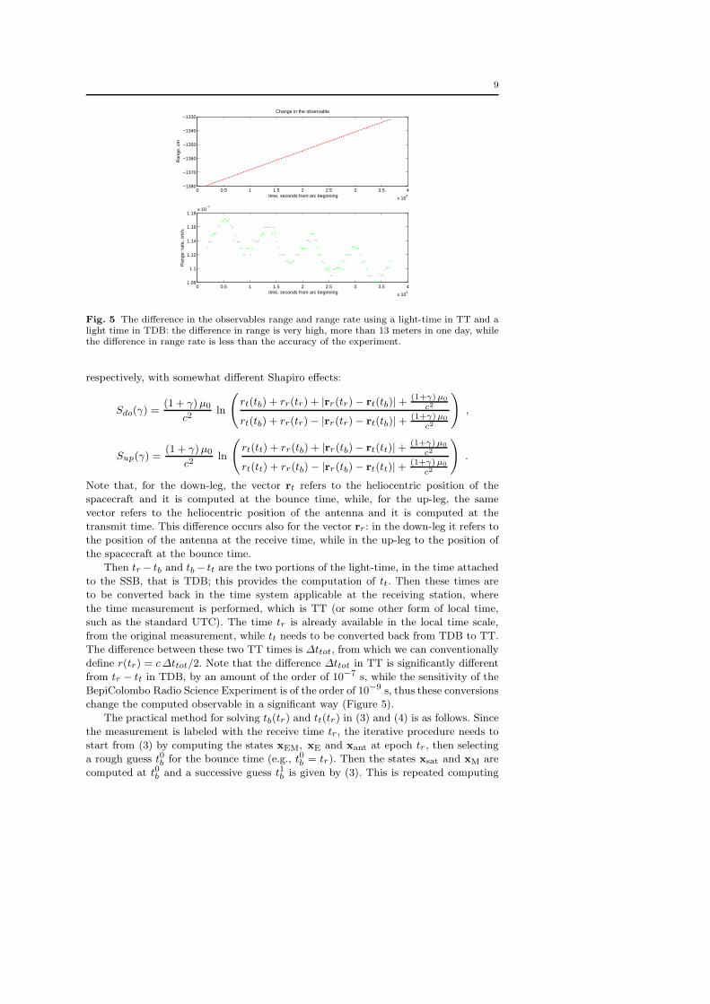
Fig. 5 The difference in the observables range and range rate using a light-time in TT and alight time in TDB: the difference in range is very high, more than 13 meters in one day, whilethe difference in range rate is less than the accuracy of the experiment.
respectively, with somewhat different Shapiro effects:
Sdo(γ) =(1 + γ) µ0
c2ln
(
rt(tb) + rr(tr) + |rr(tr) − rt(tb)| +(1+γ) µ0
c2
rt(tb) + rr(tr) − |rr(tr) − rt(tb)| +(1+γ) µ0
c2
)
,
Sup(γ) =(1 + γ)µ0
c2ln
(
rt(tt) + rr(tb) + |rr(tb) − rt(tt)| +(1+γ) µ0
c2
rt(tt) + rr(tb) − |rr(tb) − rt(tt)| +(1+γ) µ0
c2
)
.
Note that, for the down-leg, the vector rt refers to the heliocentric position of the
spacecraft and it is computed at the bounce time, while, for the up-leg, the same
vector refers to the heliocentric position of the antenna and it is computed at the
transmit time. This difference occurs also for the vector rr: in the down-leg it refers to
the position of the antenna at the receive time, while in the up-leg to the position of
the spacecraft at the bounce time.
Then tr − tb and tb − tt are the two portions of the light-time, in the time attached
to the SSB, that is TDB; this provides the computation of tt. Then these times are
to be converted back in the time system applicable at the receiving station, where
the time measurement is performed, which is TT (or some other form of local time,
such as the standard UTC). The time tr is already available in the local time scale,
from the original measurement, while tt needs to be converted back from TDB to TT.
The difference between these two TT times is ∆ttot, from which we can conventionally
define r(tr) = c ∆ttot/2. Note that the difference ∆ttot in TT is significantly different
from tr − tt in TDB, by an amount of the order of 10−7 s, while the sensitivity of the
BepiColombo Radio Science Experiment is of the order of 10−9 s, thus these conversions
change the computed observable in a significant way (Figure 5).
The practical method for solving tb(tr) and tt(tr) in (3) and (4) is as follows. Since
the measurement is labeled with the receive time tr, the iterative procedure needs to
start from (3) by computing the states xEM, xE and xant at epoch tr, then selecting
a rough guess t0b for the bounce time (e.g., t0b = tr). Then the states xsat and xM are
computed at t0b and a successive guess t1b is given by (3). This is repeated computing

10
t2b , and so on until convergence, that is, until tkb − tk−1b is smaller than the required
accuracy. This fixed point iteration to solve the implicit equation for tb is convergent
because the motion of the satellite and of Mercury, in the time tr − tb, is a small
fraction of the total difference vector. After accepting the last value of tb we start with
the states xsat and xM at tb and with a rough guess t0t for the transmit time (e.g.,
t0t = tb). Then xEM, xE and xant are computed at epoch t0t and t1t is given by (4),
and the same procedure is iterated to convergence, that is to achieve a small enough
tkt − tk−1t . This double iterative procedure to compute range is consistent with what
has been used for a long time in planetary radar, as described in (Yeomans et al. 1992).
We conventionally define r = (rdo + Sdo + rup + Sup)/2.
4.2 Range rate
After the two iterations providing at convergence tb and tt are complete, we can proceed
to compute the range rate. We shall use the following notation:
– ddtr
stands for the total derivative with respect to the receive time tr;
– ∂∂tb
stands for the partial derivative with respect to the receive time tb;
– ∂∂tt
stands for the partial derivative with respect to the receive time tt.
We rewrite the expression for the Euclidean range (down-leg and up-leg) as a scalar
product:
r2do(tr) = [xMs(tb) − xEa(tr)] · [xMs(tb) − xEa(tr)] ,
r2up(tr) = [xMs(tb) − xEa(tt)] · [xMs(tb) − xEa(tt)] ,
where xMs = xM +xsat and xEa = xEM +xE +xant. The light-time equation contains
also the Shapiro terms, thus the range rate observable contains also additive terms
dSdo/dtr and dSup/dtr, with significant effects (a few cm/s during superior conjunc-
tions). Since the equations giving tb and tt are still (3) and (4), in computing the time
derivatives, we need to take into account that tb = tb(tr) and tt = tt(tr), with non-unit
derivatives. By computing the derivative with respect to the receive time tr we obtain
d
dtr[rdo(tr) + Sdo(tr)] = rdo ·
[
∂xMs(tb)
∂tb
dtbdtr
−dxEa(tr)
dtr
]
+dSdo
dtr(5)
where
rdo =xMs(tb) − xEa(tr)
rdo(tr),
dtbdtr
= 1 −drdo(tr)/dtr + dSdo/dtr
c
and
d
dtr[rup(tr) + Sup(tr)] = rup ·
[
∂xMs(tb)
∂tb
dtbdtr
−∂xEa(tt)
∂tt
dttdtr
]
+dSup
dtr(6)
where
rup =xMs(tb) − xEa(tt)
rup(tr),
dttdtr
= 1 −drdo(tr)/dtr + dSdo/dtr
c−
drup(tr)/dtr + dSup/dtrc
.

11
The derivatives of the Shapiro effect are
dSdo
dtr=
2 (1 + γ)µ0
c2
[
(
rt(tb) + rr(tr) +(1 + γ)µ0
c2
)2
− |rr(tr) − rt(tb)|2
]
−1
(7)
[
− |rr(tr) − rt(tb)|
(
∂rt
∂tb
dtbdtr
+drr
dtr
)
+
rr(tr) − rt(tb)
|rr(tr) − rt(tb)|·
(
drr
dtr−
∂rt
∂tb
dtbdtr
) (
rt(tb) + rr(tr) +(1 + γ)µ0
c2
)
]
,
dSup
dtr=
2 (1 + γ)µ0
c2
[
(
rt(tt) + rr(tb) +(1 + γ)µ0
c2
)2
− |rr(tb) − rt(tt)|2
]
−1
(8)
[
− |rr(tb) − rt(tt)|
(
∂rt
∂tt
dttdtr
+∂rr
∂tb
dtbdtr
)
+
rr(tb) − rt(tt)
|rr(tr) − rt(tb)|·
(
∂rr
∂tb
dtbdtr
−∂rt
∂tt
dttdtr
) (
rt(tt) + rr(tb) +(1 + γ)µ0
c2
)
]
.
Note that, because of different definitions of rt and rr in the down-leg and up-leg
(Section 4.1), the term ∂rt/∂tb in the second row of (7) is exactly the same thing as
∂rr/∂tb in the second row of (8). However, the contribution of the time derivatives of
the Shapiro effect to the d tb/d tr and d tt/d tr corrective factors is small, of the order of
10−10, which is marginally significant for the BepiColombo Radio Science Experiment.
We conventionally define the range rate dr/dtr = c(1 − dtt/dtr)/2 = (drdo/dtr +
dSdo/dtr +drup/dtr +dSup/dtr)/2. These equations are compatible with the equations
in (Yeomans et al. 1992), taking into account that they use a single iteration. Equations
(7) and (8) are almost never found in the literature and has not been much used in
the processing of the past radio science experiments (Bertotti et al. 2003) because the
observable range rate is typically computed as difference of ranges divided by time;
however, for reasons explained in Section 5, these formulas are now necessary.
Since the time derivatives of the Shapiro effects contain dtb/dtr and dtt/dtr, the
equations (5) and (6) are implicit, thus we can again use a fixed point iteration. It is
also possible to use a very good approximation which solves explicitly for drdo/dtr and
then for drup/dtr, neglecting the very small contribution of Shapiro terms:
drdo
dtr= rdo·
[
∂xMs(tb)
∂tb
(
1 −dSdo/dtr
c
)
−dxEa(tr)
dtr
] [
1 +1
c
(
∂xMs(tb)
∂tb· rdo
)]
−1
,
where the right hand side is weakly dependent upon drdo/dtr only through dSdo/dtr,
thus a moderately accurate approximation could be used in the computation of dSdo/dtr,
followed by a single iteration. For the other leg
drup
dtr= rup ·
[
∂xMs(tb)
∂tb
(
1 −drdo(tr)/dtr + dSdo/dtr
c
)
−
12
∂xEa(tt)
∂tt
(
1 −drdo(tr)/dtr + dSdo/dtr + dSup/dtr
c
)
]
[
1 −1
c
(
∂xEa(tt)
∂tt· rup
)]
−1
All the above computations are in SSB with TDB; however, the frequency measure-
ments, at both tt and tr, are done on Earth, that is with a time which is TT. This
introduces a change in the measured frequencies at both ends, and because this change
is not the same (the Earth having moved by about 3 × 10⁻⁴ of its orbit) there is a
correction needed to be performed. The quantity we are measuring is essentially the
derivative of tt with respect to tr, but in two different time systems (for readability,
we use T for TT, t for TDB):
dTt
dTr=
dTt
dtt
dttdtr
dtrdTr
,
where the derivatives of the time coordinate changes are the same as the right hand
side of the differential equation giving T as a function of t in the first factor and the
inverse of the same for the last factor. However, the accuracy required is such that the
main term with the gravitational mass of the Sun µ0 and the position of the Sun x0 is
enough:
dTt
dTr=
[
1 −µ0
|xE(tt) − x0(tt)| c2−
1
2 c2
∣
∣
∣
∣
dxE(tt)
dtt
∣
∣
∣
∣
2]
dttdtr
[
1 −µ0
|xE(tr) − x0(tr)| c2−
1
2 c2
∣
∣
∣
∣
dxE(tr)
dtr
∣
∣
∣
∣
2]
−1
. (9)
Note that we do not need the LC constant term discussed in Section 2 because it
cancels in the first and last term in the right hand side of (9). The correction of the
above formula is required for consistency, but the correction has an order of magnitude
of 10−7 cm/s and is negligible for the sensitivity of the BepiColombo Radio Science
Experiment (Figure 5).
5 Numerical problems and solutions
The computation of the observables, as presented in the previous section, is already
complex, but still the list of subtle technicalities is not complete. A problem well known
in radio science is that, for top accuracy, the range rate measurement cannot be the
value dr(tr)/dtr = (drdo(tr)/dtr + dSdo/dtr + drup(tr)/dtr + dSup/dtr)/2. In fact, the
measurement is not instantaneous: an accurate measure of a Doppler effect requires
to fit the difference of phase between carrier waves, the one generated at the station
and the one returned from space, accumulated over some integration time ∆, typically
between 10 and 1000 s. Thus the observable is really a difference of ranges
r(tb + ∆/2) − r(tb − ∆/2)
∆(10)
or, equivalently, an averaged value of range rate over the integration interval
1
∆
∫ tb+∆/2
tb−∆/2
dr(s)
dtrds . (11)
13
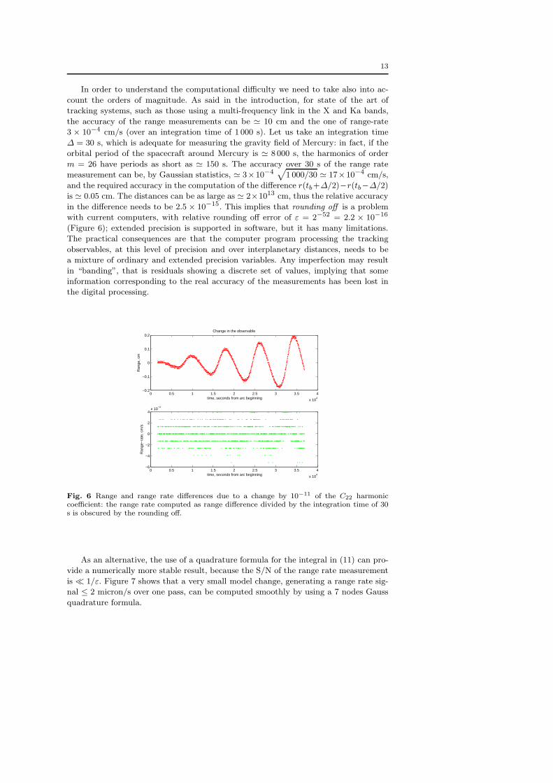
In order to understand the computational difficulty we need to take also into ac-
count the orders of magnitude. As said in the introduction, for state of the art of
tracking systems, such as those using a multi-frequency link in the X and Ka bands,
the accuracy of the range measurements can be ≃ 10 cm and the one of range-rate
3 × 10⁻⁴ cm/s (over an integration time of 1 000 s). Let us take an integration time
∆ = 30 s, which is adequate for measuring the gravity field of Mercury: in fact, if the
orbital period of the spacecraft around Mercury is ≃ 8 000 s, the harmonics of order
m = 26 have periods as short as ≃ 150 s. The accuracy over 30 s of the range rate
measurement can be, by Gaussian statistics, ≃ 3×10⁻⁴√
1 000/30 ≃ 17×10−4 cm/s,
and the required accuracy in the computation of the difference r(tb+∆/2)−r(tb−∆/2)
is ≃ 0.05 cm. The distances can be as large as ≃ 2×1013 cm, thus the relative accuracy
in the difference needs to be 2.5 × 10⁻¹⁵. This implies that rounding off is a problem
with current computers, with relative rounding off error of ε = 2−52 = 2.2 × 10⁻¹⁶
(Figure 6); extended precision is supported in software, but it has many limitations.
The practical consequences are that the computer program processing the tracking
observables, at this level of precision and over interplanetary distances, needs to be
a mixture of ordinary and extended precision variables. Any imperfection may result
in “banding”, that is residuals showing a discrete set of values, implying that some
information corresponding to the real accuracy of the measurements has been lost in
the digital processing.
0 0.5 1 1.5 2 2.5 3 3.5 4
x 104
−0.2
−0.1
0
0.1
0.2Change in the observable
time, seconds from arc beginning
Ran
ge, c
m
0 0.5 1 1.5 2 2.5 3 3.5 4
x 104
−6
−4
−2
0
2
4x 10
−4
time, seconds from arc beginning
Ran
ge−
rate
, cm
/s
Fig. 6 Range and range rate differences due to a change by 10−11 of the C22 harmoniccoefficient: the range rate computed as range difference divided by the integration time of 30s is obscured by the rounding off.
As an alternative, the use of a quadrature formula for the integral in (11) can pro-
vide a numerically more stable result, because the S/N of the range rate measurement
is ≪ 1/ε. Figure 7 shows that a very small model change, generating a range rate sig-
nal ≤ 2 micron/s over one pass, can be computed smoothly by using a 7 nodes Gauss
quadrature formula.

14
0 0.5 1 1.5 2 2.5 3 3.5 4
x 104
−0.2
−0.1
0
0.1
0.2Change in the observable
time, seconds from arc beginning
Ran
ge, c
m
0 0.5 1 1.5 2 2.5 3 3.5 4
x 104
−1.5
−1
−0.5
0
0.5
1
1.5
2x 10
−4
time, seconds from arc beginning
Ran
ge−
rate
, cm
/s
Fig. 7 Range and range rate differences due to a change by 10−11 of the C22 harmoniccoefficient: the range rate computed as an integral is smooth; the difference is marginallysignificant with respect to the measurement accuracy.
6 Conclusions
By combining the results of (Milani et al. 2010) and of this paper, we have completed
the task of showing that it is possible to build a consistent relativistic model of the dy-
namics and of the observations for a Mercury orbiter tracked from the Earth, at a level
of accuracy and self-consistency compatible with the very demanding requirements
of the BepiColombo Radio Science Experiment. In particular, in this paper we have
defined the algorithms for the computation of the observables range and range rate,
including the reference system effects and the Shapiro effect. We have shown which
computations can be performed explicitly and which ones need to be obtained from
an iterative procedure. We have also shown how to push these computations, when
implemented in a realistic computer with rounding-off, to the needed accuracy level,
even without the cumbersome usage of quadruple precision. The list of “relativistic
corrections”, assuming that we can distinguish their effects separately, is long, and we
have shown that many subtle effects are relevant to the required accuracy. However, in
the end what is required is just to be fully consistent with a post-Newtonian formula-
tion to some order, to be adjusted when necessary. Interestingly, the high accuracy of
BepiColombo radio system may require implementation of the second post-Newtonian
effects in range.
Acknowledgements The authors thank the anonymous reviewer for his constructive com-ments useful to improve the presentation of the work. The results of the research presentedin this paper, as well as in the previous one (Milani et al. 2010), have been performed withinthe scope of the contract ASI/2007/I/082/06/0 with the Italian Space Agency. BepiColombois a scientific space mission of the Science Directorate of the European Space Agency. Thework of DV was partially supported by the Czech Grant Agency (grant 202/09/0772) and theResearch Program MSM0021620860 of the Czech Ministry of Education.

15
References
Ashby and Bertotti 2009. Ashby, N., Bertotti, B.: Accurate light-time correction due
to a gravitating mass, ArXiv e-prints, 0912.2705 (2009)
Bertotti et al. 2003. Bertotti, B., Iess, L., Tortora, P.: A test of general relativity using
radio links with the Cassini spacecraft. Nature, 425, 374-376 (2003)
Damour et al. 1994. Damour, T., Soffel, M., Hu, C.: General-relativistic celestial me-
chanics. IV. Theory of satellite motion. Phys. Rev. D, 49, 618-635 (1994)
Iess and Boscagli 2001. Iess, L., Boscagli, G.: Advanced radio science instrumentation
for the mission BepiColombo to Mercury. Plan. Sp. Sci., 49, 1597-1608 (2001)
Klioner and Zschocke 2007. Klioner, S.A., Zschocke, S.: GAIA-CA-TN-LO-SK-002-1
report (2007)
Klioner 2008. Klioner, S.A.: Relativistic scaling of astronomical quantities and the
system of astronomical units. Astron. Astrophys., 478, 951–958 (2008)
Klioner et al. 2010. Klioner, S.A., Capitaine, N., Folkner, W., Guinot, B., Huang, T.
Y., Kopeikin, S., Petit, G., Pitjeva, E., Seidelmann, P. K., Soffel, M.: Units of
Relativistic Time Scales and Associated Quantities. In: Klioner, S., Seidelmann,
P.K., Soffel, M. (eds.) Relativity in Fundamental Astronomy: Dynamics, Reference
Frames, and Data Analysis, IAU Symposium, 261, 79-84 (2010)
Milani et al. 2002. Milani, A., Vokrouhlicky, D., Villani, D., Bonanno, C., Rossi, A.:
Testing general relativity with the BepiColombo radio science experiment. Phys.
Rev. D, 66, 082001 (2002)
Milani and Gronchi 2010. Milani A., Gronchi G.F.: Theory of orbit determination.
Cambridge University Press (2010)
Milani et al. 2010. Milani, A., Tommei, G., Vokrouhlicky, D., Latorre, E., Cicalo, S.:
Relativistic models for the BepiColombo radioscience experiment. In: Klioner, S.,
Seidelmann, P.K., Soffel, M. (eds.) Relativity in Fundamental Astronomy: Dynam-
ics, Reference Frames, and Data Analysis, IAU Symposium, 261, 356-365 (2010)
Moyer 2003. Moyer, T.D.: Formulation for Observed and Computed Values of Deep
Space Network Data Types for Navigation. Wiley-Interscience (2003)
Shapiro 1964. Shapiro, I.I.: Fourth test of general relativity. Phys. Rev. Lett., 13, 789-
791 (1964)
Soffel et al. 2003. Soffel, M., Klioner, S.A., Petit, G., Kopeikin, S.M., Bretagnon, P.,
Brumberg, V.A., Capitaine, N., Damour, T., Fukushima, T., Guinot, B., Huang,
T.-Y., Lindegren, L., Ma, C., Nordtvedt, K., Ries, J.C., Seidelmann, P.K., Vokrouh-
licky, D., Will, C.M., Xu, C.: The IAU 2000 resolutions for astrometry, celestial
mechanics, and metrology in the relativistic framework: explanatory supplement.
Astron. J., 126, 2687-2706 (2003)
Teyssandier and Le Poncin-Lafitte 2008. Teyssandier, P., Le Poncin-Lafitte, C.: Gen-
eral post-Minkowskian expansion of time transfer functions. Class. Quantum Grav.,
25, 145020 (2008)
Will 1993. Will, C.M.: Theory and experiment in gravitational physics. Cambridge
University Press (1993)
Yeomans et al. 1992. Yeomans, D. K., Chodas, P. W., Keesey, M. S., Ostro, S. J.,
Chandler, J. F., Shapiro, I. I.: Asteroid and comet orbits using radar data. Astron.
J., 103, 303-317 (1992)


![BepiColombo/MMO: MDP MMO-SWG #3 [March 2006] -1- C. Noshi/RASC, Kyoto Univ. MMO Mercury Magnetospheric Orbiter MDP (Mission Data Processor) for BepiColombo](https://img.pdfslide.net/doc/110x75/56649ef05503460f94c00b22/bepicolombommo-mdp-mmo-swg-3-march-2006-1-c-noshirasc-kyoto-univ.jpg)