Embed Size (px)
Citation preview

Lighting and Materials for Real-Time Game Engines
T O B I A S K R U S E B O R N
Master of Science Thesis Stockholm, Sweden 2009

Lighting and Materials for Real-Time Game Engines
T O B I A S K R U S E B O R N
Master’s Thesis in Computer Science (30 ECTS credits) at the School of Computer Science and Engineering Royal Institute of Technology year 2009 Supervisor at CSC was Lars Kjelldahl Examiner was Lars Kjelldahl TRITA-CSC-E 2009:085 ISRN-KTH/CSC/E--09/085--SE ISSN-1653-5715 Royal Institute of Technology School of Computer Science and Communication KTH CSC SE-100 44 Stockholm, Sweden URL: www.csc.kth.se
Abstract The aim of this thesis was to study and implement advanced
real-time rendering techniques for complex materials such as
human skin. The project included investigation on how to adapt
and simplify complex skin rendering models to fit current game
engines. Also, the task included looking into recent research on
spherical harmonics and wavelets. The goal was to determine
whether they can be used to represent both diffuse and specular
reflection from an environment lighting in a real time game.
Subsurface scattering, Gaussian shadow mapping and
representing lighting by the use of spherical harmonics and
wavelets, are a few of the used techniques in this project. The
results of this thesis show that it is possible to render realistic
human skin in real time at a low cost. When wavelets are
combined with skin rendering techniques, a high-quality method
is established for rendering complex materials from environment
light. This thesis was written at Digital Illusions and CSC at the
Royal Institute of Technology in Stockholm in the spring of
2009.
Ljussättning och material för spelmotorer i realtid
Sammanfattning
Syftet med detta examensarbete var att studera och
implementera avancerade renderingstekniker för komplexa
material, såsom människohud. Projektet innefattade en
utredning av hur man kan förändra och förenkla komplicerade
hudrenderingsmodeller för att de ska passa in i dagens
spelmotorer. I uppgiften ingick även studier inom den senaste
forskningen om klotytfunktioner och wavelets. Målet var att
avgöra om dessa tekniker kan användas för att representera både
diffus och spekulär reflektion från omgivningsljus i realtid.
Subsurface scattering, Gaussian shadow mapping och
omgivningsljussättning med hjälp av klotytfunktioner och
wavelets, är några av de använda teknikerna i detta projekt.
Resultaten av detta examensarbete visar att det är möjligt att
rendera realistisk hud i realtid och till en låg kostnad. När
wavelets kombineras med hudrenderingstekniker, skapas en
högkvalitativ metod för att rendera komplexa material från
omgivningsljus. Detta examensarbete utfördes åt Digital
Illusions och CSC vid Kungliga Tekniska Högskolan i
Stockholm våren 2009.

Acknowledgements I would like to thank everyone who has supported me during the work with this thesis – in the
great as well as in the small. I'm grateful to my supervisor and examiner Lars Kjelldahl, for
helping me plan and execute the thesis. Special thanks to my supervisors Per Einarsson and
Daniel Johansson for their time, their patience and for sharing their knowledge. Finally I
would like to thank Digital Illusions for giving me the opportunity to do my thesis at their
company.

Contents
1. Introduction ..................................................................................................................................... 1
1.1 Problem definition ................................................................................................................... 1
1.2 Objective ................................................................................................................................. 1
1.3 Delimitations ........................................................................................................................... 1
1.4 Methods ................................................................................................................................... 2
2. Skin rendering ................................................................................................................................. 3
2.1 Theory ..................................................................................................................................... 3
2.1.1 Specular and diffuse reflections in skin ......................................................................... 4
2.1.2 Diffuse approximation ................................................................................................... 5
2.1.4 Extending translucent shadow maps ............................................................................. 8
2.1.5 EA contribution ............................................................................................................ 10
2.2 Implementation and results.................................................................................................... 14
2.2.1 Shadows ....................................................................................................................... 14
2.2.2 Diffuse Illumination ...................................................................................................... 15
2.2.3 Modified Translucent Shadow Maps ........................................................................... 17
2.2.4 Final skin rendering algorithm ..................................................................................... 17
2.3 Conclusions ........................................................................................................................... 18
3. Environment lighting ..................................................................................................................... 19
3.1 The Median Cut Algorithm ................................................................................................... 19
3.1.1 Theory .......................................................................................................................... 19
3.1.3 Conclusions .................................................................................................................. 21
3.2 Spherical Harmonics ............................................................................................................. 22
3.2.1 Theory .......................................................................................................................... 22
3.2.2 Implementation and results ......................................................................................... 25
3.2.3 Conclusions .................................................................................................................. 34
3.3 Wavelets ................................................................................................................................ 34
3.3.1 Theory .......................................................................................................................... 34
3.3.2 Implementation and results ......................................................................................... 41
3.3.3 Conclusions .................................................................................................................. 55
4. Evaluation of the results ................................................................................................................ 56
5. Glossary ......................................................................................................................................... 57
References ............................................................................................................................................. 59

Appendix ............................................................................................................................................... 61
Appendix 1. Normal shadow map ................................................................................................. 61
Appendix 2. Shadow map with a 4x4 uniform filter ..................................................................... 62
Appendix 3. Shadow map with a 5x5 Gaussian filter ................................................................... 63
Appendix 4. Diffuse light from St. Peter's Basilica, Rome ........................................................... 64
Appendix 5. Diffuse light with applied subsurface scattering ....................................................... 65
Appendix 6. Diffuse light from The Uffizi Gallery, Florence ....................................................... 66
Appendix 7. Diffuse light with applied subsurface scattering ....................................................... 67
Appendix 8. Diffuse light from Eucalyptus Grove, UC Berkeley ................................................. 68
Appendix 9. Diffuse light with applied subsurface scattering ....................................................... 69
Appendix 10. Diffuse light from Galileo's Tomb, Santa Croce, Florence .................................... 70
Appendix 11. Diffuse light with applied subsurface scattering. .................................................... 71
Appendix 4. Specular reflection - Soho wavelets, BRDF - Cook-Torrance ................................. 72
Appendix 5. Specular reflection - Soho wavelets, BRDF - Kelemen/Szirmay-Kalos .................. 73
Appendix 6. Specular reflection - Halo3, BRDF - Cook-Torrance ............................................... 74
Appendix 15. Specular reflection represented by 16 Soho wavelets coefficients ......................... 75
Appendix 16. Specular reflection represented by 32 Soho wavelets coefficients ......................... 76
Appendix 17. Specular reflection represented by 64 Soho wavelets coefficients ......................... 77
Appendix 18. Specular reflection represented by 256 Soho wavelets coefficients ....................... 78
Appendix 19. Specular reflection represented by 512 Soho wavelets coefficients ....................... 79

1
1. Introduction Computer and console games are part of one of the largest industries today. As a result the
game developing companies take on more advanced techniques to achieve more detailed and
realistic graphics, in order to attract the consumers. However difficulties arise when trying to
lighten material in a physically correct way and in real time, because of the complexity of the
materials, and the way we can represent light.
1.1 Problem definition Human skin is one of the most complex materials since it includes wrinkles, freckles, and
scars etc. By using the 3D scanners of today, these facial details can be captured. However the
skin appearance will still look artificial due to a lack of subsurface scattering, which brings
about most of the lighting colors in our skin. Sub-surface scattering is the main means of how
the light is reflected from the skin. For that reason, ignoring sub-surface scattering, results in
unnatural appearance.
The most common lighting model in computer games is diffuse shading with a specular
reflection. The last years diffuse reflection has been able to be represented by environment
lighting by methods such as spherical harmonics, but the specular reflection is still restricted
to a few point lights. Representing specular reflection from environment lighting with other
basis, such as wavelets or new techniques with spherical harmonics, could be an option to
point lights.
Recent research has demonstrated convincing results of real-time rendering of human skin
and faces. These techniques have adapted models including geometric details and subsurface
scattering shadings, which previously only have been possible in offline rendering. However,
they might not be applicable to current games, which consist of many characters and complex
scenes.
1.2 Objective The aim of this thesis was to study and implement advanced real-time rendering techniques
for complex materials such as human skin. The project included investigation on how to adapt
and simplify complex skin rendering models to fit current game engines. Also, the task
included looking into recent research on spherical harmonics and wavelets. The goal was to
determine whether they can be used to represent both diffuse and specular reflection from an
environment lighting in a real time game. In particular, focus was put on the following areas:
Implementing real-time skin rendering based on the current state of the art techniques;
investigating how to blend different rendering models based on camera distance and scene
complexity; and evaluation of which aspects of current techniques are most important in order
to achieve photo-real quality (shading models, geometrics, complexity, lighting representation
etc).
1.3 Delimitations There are many different types of models for lighting of materials. This thesis will primarily
treat models suited for computer and console games.

2
1.4 Methods This thesis has been executed by the means of research from papers and books followed by
implementation of different techniques in C++ and Direct3D 10.0. Subsurface scattering,
modified translucent shadow mapping, diffuse approximation, complex BRDF, along with
representing lighting by the use of spherical harmonics, Haar wavelets and Soho wavelets are
a few of the used techniques in this project.
3
2. Skin rendering Many materials are difficult to render in a realistic way. Human skin is one of the most
complex ones since it includes wrinkles, freckles, and scars etc. By using the 3D scanners of
today, these facial details can be captured. However the skin appearance will still look
artificial due to a lack of subsurface scattering, which brings about most of the lighting
colours in our skin. The Lambertian model, which is the most common technique used for
rendering standard materials, is designed for solid surfaces with little or no subsurface
scattering [BasriJacobs03]. When using this technique for more complex materials, the
outcome is most often unnatural because of the usage of the normal and diffuse map for
rendering. In other words, the Lambertian lighting model can’t produce realistic faces.
The main difference between skin and other materials depends on the different reflection
paths of light. Light that meets skin, moves beneath the top skin surface and scatters and thus
some of the light is absorbed in one spot and emitted elsewhere. In other words, the human
skin has several layers with different translucency, whereas the standard model is based on the
fact that light scatters at the surface and are equal in all directions. This part of the report
describes the theory of subsurface scattering and includes specific information on how the
Doug Jones demo is implemented [NVIDIA07, d'EonGPUGems07, d'EonGDC07,
d'EonEurographics07]. By the end of this chapter, result from the implementation; using an
approximation method by John Hable, George Borshukov, and Jim Hejl, which is being
presented in the next book of the ShaderX series, will be described.
2.1 Theory When light hits the surface of an object, some of it is transferred into the surface by refraction
or transmission, while the rest is scattered from the surface. The parts of the light that are
transferred into the object can be absorbed or undertake additional scattering. Any
discontinuities in the object, such as air bubbles or density variations, may cause the light to
be scattered. Some of the scattered light is reflected through the surface and gives the surface
color from the inside; this is called subsurface scattering. In some materials the scattering is
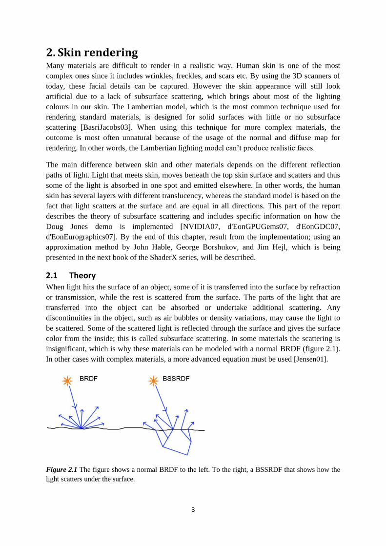
insignificant, which is why these materials can be modeled with a normal BRDF (figure 2.1).
In other cases with complex materials, a more advanced equation must be used [Jensen01].
Figure 2.1 The figure shows a normal BRDF to the left. To the right, a BSSRDF that shows how the
light scatters under the surface.

4
The equation of the bidirectional surface scattering reflectance distribution function
(BSSRDF) can be expressed as followed [Jensen01]:
𝑆 𝑥𝑖 ,𝑤𝑖 , 𝑥0 ,𝑤𝑜 =𝑑𝐿(𝑥0 ,𝑤0)
𝑑𝛷 𝑥𝑖 ,𝑤 𝑖 (2.1)
L is the outgoing radiance, Φ is the incident flux, xi and xo is the ingoing and outgoing point
and w is the ingoing and outgoing direction. The normal BRDF is an approximation of the
BSSRDF, which assumes that the ingoing and outgoing point is the same. To calculate a
BSSRDF is quite complicated since all incoming directions as well as an area A must be
integrated. The outgoing radiance can be described by the double integral presented below
[Jensen01].
𝐿𝑜 𝑥𝑜 ,𝑤𝑜 = 𝑆 𝑥𝑖 ,𝑤𝑖 , 𝑥0,𝑤𝑜 𝐿𝑖 𝑥𝑖 ,𝑤𝑖 𝑑𝑤𝑖𝑑𝐴(𝑥𝑖)𝑙
2𝜋
𝑙
𝐴 (2.2)
2.1.1 Specular and diffuse reflections in skin
The specular term of skin is much easier to represent than the diffuse term. This is based on
the fact that specular light is reflected directly and isn't absorbed by the surface. The specular
light in human skin only reflects six percent of the whole light spectrum [d'EonEuros07]. The
topmost layer of the skin is constituted of a thin oil layer and can be modeled by a BRDF.
Furthermore the oil layer doesn't give out a mirror like reflection because of the roughness of
the skin. This roughness can be described by a more complicated BRDF [d'EonGPU07].
To calculate specular reflections in skin, modern programmers use the Blinn-Phong model.
This model results in an inaccurate approximation since it outputs more energy than it
receives and moreover fails to capture increased specularity at grazing angles. The use of a
more precise physical base reflectance model can improve the quality at a cost of a few extra
shader instructions [d'EonGPU07].
According to Eugene d’Eon and David Luebke it's possible to use the Kelemen/Szirmay-
Kalos for describing the specular term [Kelemen01]. This model is very similar to the Cook-
Torrance method, which can be described by equation 2.7 [CookTo81].
𝑔 = 1+ 𝑓0
1+ 𝑓0
2
+ 𝑉 ∙ 𝐻 2 − 1, 𝑟 =𝑉∙𝐻∗ 𝑔−𝑉∙𝐻 −1
𝑉∙𝐻∗ 𝑔+𝑉∙𝐻)+1 , 𝛾 =
2(𝑁∙𝐻)
𝑉∙𝐻 (2.3)
𝐷 =1
𝑚2 𝑁∙𝐻 4 𝑒−
1− 𝑁∙𝐻 2
𝑚 2 𝑁 ∙𝐻 2 (2.4)
𝐹 =
𝑔−𝑉∙𝐻 2
𝑔+𝑉∙𝐻 2∗ 1+𝑟2
2 (2.5)
𝐺 = 𝑚𝑖𝑛 𝛾 𝑁 ∙ 𝑉 , 𝛾 𝑁 ∙ 𝐿 (2.6)
CookTorrance𝑠𝑝𝑒𝑐 = 𝑁 ∙ 𝐿 + 𝐷𝐺𝐹/𝜋(𝑁 ∙ 𝑉) (2.7)

5
The m value corresponds to the roughness in the interval 0.1, 1 , N is the surface normal, V is
the view vector and L is direction of the light. The F stands for the Fresnel term and describes
the behavior of light when moving between media of different refractive indices.
Assuming that the oil layer of the skin functions similarly to a metal surface, the Schlick
approximation method can be used instead of the Fresnel equation [Schlick94]. When dealing
with different kinds of materials however, the original Fresnel equation gives significantly
better result than the Schlick model [Schlick94].
𝐹 = 𝑓0 + 1 − 𝑓0 1 − 𝑁 ∙ 𝑉 5 (2.8)
The formula set above is the Schlick approximation. The parameter f0 comes from Beers Law
and is based on a refraction index value of 1.4 for the skin. G is the geometric attenuation
term and D is the distribution term [CookTo81].
2.1.2 Diffuse approximation
When light hits highly scattered media, light distribution tends to become isotropic
[Jensen01]. Each beam of light that hits the surface is likely to blur the light distribution and
thus, the light is uniformly spread over the surface area. To calculate the diffuse light, it's
required to solve the double integral (2.2), which is often too expensive to apply in real-time
games. The diffuse approximation method can be used instead. By applying a diffuse profile
it’s accordingly possible to approximate diffuse light reflections underneath the surface in
translucent material. [d'EonGPU07, ATI04]
The diffuse profile demonstrates how light scatters across a radial distance from its hit point,
which is comparable to when a white, thin laser beam illuminates a flat surface in a dark room
[d'EonGPU07]. When the laser beam hits a flat wall, some of the light relocates beneath the
surface, scatters and is reflected from the surface near the hit point. Furthermore the diffuse
profile tells us how much light emerges as a function of the angle and distance from the laser
center. If the material is uniform, the scattering of the light is the same in all directions and
the angle of the light is irrelevant. The diagram in figure 2.2 (a) shows that each color has its
own profile; red light scatters more than green and blue light, and therefore the red color in
the image (b) is intensified the further away we get from the hit point. [d'EonGPU07,
d'EonGDC07].
Source: GPU Gems 3
Figure 2.2 Rendering with diffusion profiles. Red light scatters more than green and blue light (a), and
thus, the red color is intensified the further away we get from the hit point (b).

6
When rendering material by the application of a diffuse profile, all incoming light converge at
the surface point before spreading to create the exact shape of the profile. Adjacent neighbors
are affected by each other’s colors and the translucent appearance is the sum of their own and
all neighborly colors. In cases of skin rendering the incoming light quickly becomes diffuse.
The incoming light direction is lost almost immediately, and consequently only the total
amount of light in one point is relevant for the diffused light. The amount of light that is
scattered is decided by the diffuse profile. Each type of material requires a different diffuse
profile to be rendered accurately. Complex matters, such as skin, contain various layers which
differ in design and structure i.e. different diffuse profiles [d'EonGPU07].
The main methods for calculating diffuse profiles today are those presented by Henrik Wann
Jensen and Donner and Jensen, 2001 and 2005 respectively [Jensen01, DonnerJensen05].
Wann Jensen established a way of computing profiles using a dipole equation, while Donner
and Jensen introduced the so called multipole theory [Donner05]. The visual appearances can
differ a lot depending on which of these two methods you use. For example, the single dipole
equation cannot capture the combined reflectance of a thin, narrowly scattering epidermis
layer on top of a widely scattering dermis layer (figure 2.3). Accordingly the multipole
method is needed to describe the subsurface scattering of skin [d'EonGPU07].
Figure 2.3 The figure shows how light scatters underneath the human skin.
A sum-of-Gaussians for diffusion profile.
Eugene d’Eon and David Luebke found that the dipole curve plotted for the diffuse profile,
can be approximated by summarizing a number of Gaussians functions 𝑒−𝑟2
[d'EonGPUGems07, d'EonGDC07, d'EonEurographics07]. To be more precise, six Gaussians
are needed to accurately match the three-multilayer profile given for skin by Donner and
Jensen. For single layer materials, four Gaussians are enough to fit most profiles. To fit
Gaussians to a diffusion profile 𝑅 𝑟 , we minimize formula 2.9:
𝑟 𝑅 𝑟 − 𝑤𝑖𝐺 𝑣𝑖 , 𝑟 𝑘𝑖=1
2𝑑𝑟
∞
0 (2.9)
7
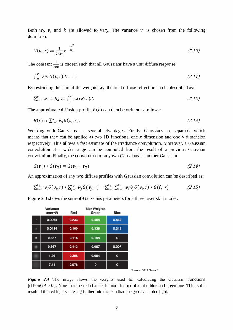
Both 𝑤𝑖 , 𝑣𝑖 and 𝑘 are allowed to vary. The variance 𝑣𝑖 is chosen from the following
definition:
𝐺 𝑣𝑖 , 𝑟 ≔1
2𝜋𝑣𝑖𝑒−−𝑟2
2𝑣𝑖 (2.10)
The constant 1
2𝜋𝑣 is chosen such that all Gaussians have a unit diffuse response:
2𝜋𝑟𝐺 𝑣, 𝑟 𝑑𝑟 = 1∞
𝑖=1 (2.11)
By restricting the sum of the weights, 𝑤𝑖 , the total diffuse reflection can be described as:
𝑤𝑖 = 𝑅𝑑 ≔ 2𝜋𝑟𝑅 𝑟 𝑑𝑟∞
0𝑘𝑖=1 (2.12)
The approximate diffusion profile 𝑅 𝑟 can then be written as follows:
𝑅(𝑟) ≈ 𝑤𝑖𝐺 𝑣𝑖 , 𝑟 ,𝑘𝑖=1 (2.13)
Working with Gaussians has several advantages. Firstly, Gaussians are separable which
means that they can be applied as two 1D functions, one 𝑥 dimension and one 𝑦 dimension
respectively. This allows a fast estimate of the irradiance convolution. Moreover, a Gaussian
convolution at a wider stage can be computed from the result of a previous Gaussian
convolution. Finally, the convolution of any two Gaussians is another Gaussian:
𝐺 𝑣1 ∗ 𝐺 𝑣2 = 𝐺 𝑣1 + 𝑣2 (2.14)
An approximation of any two diffuse profiles with Gaussian convolution can be described as:
𝑤𝑖𝐺 𝑣𝑖 , 𝑟 ∗ 𝑤 𝑗𝐺(𝑘2𝑗=1
𝑘1𝑖=1 𝑣 𝑗 , 𝑟) = 𝑤𝑖𝑤 𝑗𝐺 𝑣𝑖 , 𝑟 ∗ 𝐺(𝑣 𝑗 , 𝑟)
𝑘2𝑗=1
𝑘1𝑖=1 (2.15)
Figure 2.3 shows the sum-of-Gaussians parameters for a three layer skin model.
Source: GPU Gems 3
Figure 2.4 The image shows the weights used for calculating the Gaussian functions
[d'EonGPU07]. Note that the red channel is more blurred than the blue and green one. This is the
result of the red light scattering further into the skin than the green and blue light.

8
Texture-space diffusion
Borshukov and Lewis (2003) introduced a new technique called texture-space diffusion for
rendering faces in the movie The Matrix [Borshukov03]. Their method is based on rendering
the diffuse illumination of the geometry to a texture light map using the texture coordinates as
positions [Green04]. The texture is a 2D image representing the light at the object. A
convolution operation (blur) is performed on the texture. This diffuse light is then added
together with the specular light for the finishing skin color. Another possibility is to render
shadows to the light map using shadow maps before incorporating a blur. This handles the
problems with hard edges, that arise from shadow mapping. The algorithm for texture space
diffusion using the Gaussian blur for the convolution is as followed [d'EonGPU07].
1 Render shadows using shadow maps
2 Render irradiance into the light map
3 For each Gaussian used for the diffusion approximation
4 Perform a separable blur pass in 𝑈
5 Perform a separable blur pass in 𝑉
6 Render the mesh using the light map
Pre and post-scattering
When working with texture space diffusion, two options are available to determine the
finishing color of the skin. The first option is to accomplish the blur with a light color,
normally white, and then multiply it by the diffuse color map to get the desired skin tone. The
diffuse color is not used in the irradiance texture computation but multiplied later. The
advantage of this post scattering method is that all details in the diffuse color map are
maintained. However, this method doesn't create any color bleeding of the skin. To obtain
color bleeding the irradiance and the color map should be combined before convolution takes
place. This technique is called pre scattering [d'EonGPU07].
Since it's important to maintain all details in the texture, the hybrid version of the pre and post
scattering methods is preferable. The hybrid method is probably the most physically correct
method and is used in the Doug Jones demo[NVIDIA07]. For the Adrianne demo the diffuse
map only affects incoming light and less outgoing light [NVIDIA06]. The teqhnique signifies
that parts of the diffuse color is applied before the scatter take place and the rest is multiplied
directly afterwards. This results in bleeding in the image to a certain extent, at the same time
as the texture details remain. This can be accomplished by multiplying the lighting with
[pow(diffuseColor, mixValue)] before the blur and with pow(diffuseColor, 1 − mixValue)
afterwards. mixValue determines the amount of color that should be added before and after
scattering [d'EonGPU07].
2.1.4 Extending translucent shadow maps
In Texture-space diffusion, some regions that are close to each other in Euclidean space can
be far away from each other in texture space. This means that for example, ears and noses,
can't capture light transmitters from both sides, and therefore, scattering can only be observed
in the part that is pointed to the direction of light. E. d’Eon and D. Luebke use a technique

9
which is based on modifying translucent shadow maps (TSM) to solve this problem
[d'EonGPU07, d'EonEuro07]. The map can be studied further in figure 2.5.
Source: GPU GEMS 3
Figure 2.5 E. d’Eon, D. Luebke modified translucent shadow map.
A normal TSM render the depth, irradiance and the surface normal to subsequently store these
quantities for the surface facing the light at each pixel in the texture. The technique stores the
depth and the (𝑢, 𝑣) coordinates of the light facing the surface. In run time, each surface that
is within the shadow, can study the texture to find the distance through the object toward the
light, and access the convolved version of irradiance on the light facing surface. In skin
rendering, the scattering will not be noticeable if the distance 𝑚 is large, but if the distance is
small a red glow will be visible from the shadow area (figure 2.6).
Source: GPU GEMS 3
Figure 2.6 The image shows the function of global scattering through thin regions.
The point 𝐶 is a shadow location on an object, the TSM provides the distance 𝑚 and the
(𝑢, 𝑣) coordinates for the point 𝐴, on the surface toward the light. We want to estimate the
scattering light exiting at point 𝐶, which is the convolution of irradiance 𝐴 through the object
individually for each sample. However, this can be quite costly to apply in real time.
Computing this scattering effect for point 𝐵 is easier than to compute it for point 𝐶. For small
angels, 𝐵 will be a close approximation to 𝐶 and for large angels, the Fresnel and the cosine
term will hide the error of the approximation. The scattering at 𝐵 from 𝐴 can be computed at
several samples at a distance 𝑟 from 𝐴.
𝑅( 𝑟2 + 𝑑2) = 𝑤𝑖𝐺 𝑣𝑖 , 𝑟2 + 𝑑2 = 𝑤𝑖𝑒−𝑑2
2𝑣𝑖𝑘𝑖=1 𝐺(𝑣𝑖 , 𝑟)𝑘
𝑖=1 (2.16)

10
2.1.5 EA contribution
The Doug Jones demo (figure 2.7), by E. d’Eon, D. Luebke, has put high expectations on skin
rendering in real time, with its high quality and realistic appearance [NVIDIA07]. However
one must have in mind that in modern computer games many objects besides the human face
must be rendered. Normally, the game engine has to render an entire world at each frame,
which means that just a small fraction of the time is reserved for the skin shader. Furthermore
the demo runs quite slowly, although it's driven on a top notch computer. This underlines the
fact that the technique needs to be scaled down, to work in next generation games.
Source: NVIDIA
Figure 2.7 Picture taken from Dough Jones Head demo. The demo puts high expectations on skin
rendering in terms quality of the appearance.
As part of new research, John Hable, George Borshukov, and Jim Hejl from EA have used the
same technique as E. d’Eon, D. Luebke. By performing a number of modifications, they have
managed to scale it down, but still retain a high quality to fit the technique of current
generation consoles, such as Playstation 3 and Xbox 360.
Simulating the Gaussian blur
The bottleneck with Dough Jones implementation is the Gaussian blur pass. Since the
Gaussian blur is separable, in one horizontal and one vertical pass respectively, each blur pass
is actually representing two passes. To fit the diffuse profile for human faces, six blur passes
and 7 ∗ 2 taps for each blur, are required for. The total cost for the Gaussian blur is 14 ∗ 6 =
84 taps, and later on an additional cost for reading from the six textures will arise. The E.
d’Eon, D. Luebke technique, for skin rendering, fit the diffuse profile almost precisely, but is
too expensive. The research by EA determines, that it is possible to get almost the same result
with significantly improved performance, by using a carefully chosen sampling pattern. The
teqhnique is built on the use of two rings; where each ring is divided into six sections at a total
cost of 12 sections. This will create a full kernel with 12 jitter samples and the weights of the

11
kernels multiplied by six, one for each Gaussian blur. The samples are finally combined in an
offline process, into a single kernel, representing the whole Gaussian blur process.
blurJitteredWeights[13] =
{
{ 0.220441, 0.437000, 0.635000 },
{ 0.076356, 0.064487, 0.039097 },
{ 0.116515, 0.103222, 0.064912 },
{ 0.064844, 0.086388, 0.062272 },
{ 0.131798, 0.151695, 0.103676 },
{ 0.025690, 0.042728, 0.033003 },
{ 0.048593, 0.064740, 0.046131 },
{ 0.048092, 0.003042, 0.000400 },
{ 0.048845, 0.005406, 0.001222 },
{ 0.051322, 0.006034, 0.001420 },
{ 0.061428, 0.009152, 0.002511 },
{ 0.030936, 0.002868, 0.000652 },
{ 0.073580, 0.023239, 0.009703 },
};
blurJitteredSamples[13] =
{
{ 0.000000, 0.000000 },
{ 1.633992, 0.036795 },
{ 0.177801, 1.717593 },
{ -0.194906, 0.091094 },
{ -0.239737, -0.220217 },
{ -0.003530, -0.118219 },
{ 1.320107, -0.181542 },
{ 5.970690, 0.253378 },
{ -1.089250, 4.958349 },
{ -4.015465, 4.156699 },
{ -4.063099, -4.110150 },
{ -0.638605, -6.297663 },
{ 2.542348, -3.245901 },
};
The first sample 𝑢, 𝑣 = (0,0) represents the incoming and directly outgoing light and the
following six samples correspond to the middle-level scattering. The last six samples stand for
the wide-level scattering, and as can be seen on the weights {red, green, blue}, they are
mainly used for the red light. The result is different blurs for each color channel, which can be
done in one single pass. The cost of reading from 6 textures is eliminated, since the final pixel
shader only reads from one texture.
Light map optimization
When performing the blur on a light map, the blur is applied to the whole texture. This is not
necessary, instead we want to blur all front facing polygons. The polygons poke a hole in the
depth buffer and use high-z to perform the blur. During the light map rendering, we can set
the depth to 𝑁 ∙ 𝑉 ∗ 0.5 + 0.5 (figure 2.8). With this formula, all points on the face that are
turned directly to the camera will have a depth of 1 and the points which are not facing the
camera will have an output of 0 [Borshukov03, Borshukov05].
Source: EA
Figure 2.8 Image taken from the John Hable, George Borshukov, and Jim Hejl upcoming paper on
fast skin shading. The black area will not be blurred because its area will not be rendered. The gray
area is not visible from the camera view, and thus this area will be blurred.
12
High quality shadow filtering
There are many techniques for rendering shadows. One of the most popular methods are
shadow mapping, which is a two step technique:
1. In the first step the whole scene is rendered from light position. The depth of each
pixel is saved in a texture automatically by the use of a depth buffer.
2. The second step includes rendering of the scene from view position, with the shadow
map projected from the light on the scene as a projection texture. Each pixel that is
rendered is comparable to the depth in the shadow map. If the depth from the light is
shorter than from the eye position, the pixel is in shade.
Shadow mapping has several advantages compared to other shadow methods [GDC08]. For
example the creation of a shadow map is proceeded in linear time and the access time is
measured to O(1). The disadvantage is that the shadow resolution depends on the resolution
of the shadow map texture.
There are many advanced techniques for smooth shadows using shadow maps, the most
prominent are CSM (Convolution Shadow Maps), VSM(Variance Shadow Maps), ESM
(Exponential Shadow Maps) and can be combined with SATs [Crow84] for arbitrary
smoothness [GDC08]. These techniques include a complex rendering step and furthermore
the methods cause different artifacts. By using a simple Percentage closer filter we can almost
get the same result as the advanced techniques, with much less complexity.
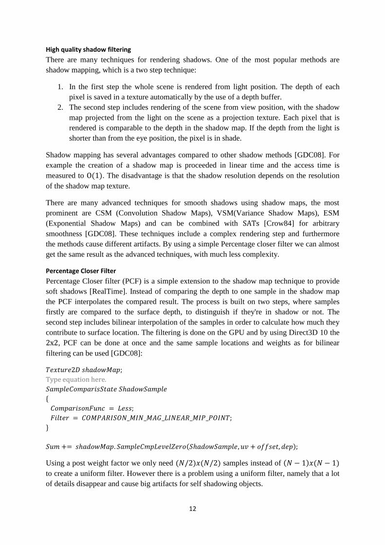
Percentage Closer Filter
Percentage Closer filter (PCF) is a simple extension to the shadow map technique to provide
soft shadows [RealTime]. Instead of comparing the depth to one sample in the shadow map
the PCF interpolates the compared result. The process is built on two steps, where samples
firstly are compared to the surface depth, to distinguish if they're in shadow or not. The
second step includes bilinear interpolation of the samples in order to calculate how much they
contribute to surface location. The filtering is done on the GPU and by using Direct3D 10 the
2x2, PCF can be done at once and the same sample locations and weights as for bilinear
filtering can be used [GDC08]:
𝑇𝑒𝑥𝑡𝑢𝑟𝑒2𝐷 𝑠𝑎𝑑𝑜𝑤𝑀𝑎𝑝;
Type equation here.
𝑆𝑎𝑚𝑝𝑙𝑒𝐶𝑜𝑚𝑝𝑎𝑟𝑖𝑠𝑆𝑡𝑎𝑡𝑒 𝑆𝑎𝑑𝑜𝑤𝑆𝑎𝑚𝑝𝑙𝑒
{
𝐶𝑜𝑚𝑝𝑎𝑟𝑖𝑠𝑜𝑛𝐹𝑢𝑛𝑐 = 𝐿𝑒𝑠𝑠;
𝐹𝑖𝑙𝑡𝑒𝑟 = 𝐶𝑂𝑀𝑃𝐴𝑅𝐼𝑆𝑂𝑁_𝑀𝐼𝑁_𝑀𝐴𝐺_𝐿𝐼𝑁𝐸𝐴𝑅_𝑀𝐼𝑃_𝑃𝑂𝐼𝑁𝑇;
}
𝑆𝑢𝑚 += 𝑠𝑎𝑑𝑜𝑤𝑀𝑎𝑝. 𝑆𝑎𝑚𝑝𝑙𝑒𝐶𝑚𝑝𝐿𝑒𝑣𝑒𝑙𝑍𝑒𝑟𝑜 𝑆𝑎𝑑𝑜𝑤𝑆𝑎𝑚𝑝𝑙𝑒,𝑢𝑣 + 𝑜𝑓𝑓𝑠𝑒𝑡, 𝑑𝑒𝑝 ;
Using a post weight factor we only need (𝑁/2)𝑥(𝑁/2) samples instead of 𝑁 − 1 𝑥(𝑁 − 1)
to create a uniform filter. However there is a problem using a uniform filter, namely that a lot
of details disappear and cause big artifacts for self shadowing objects.

13
Figures 2.9-2.10 illustrate the difference between a normal uniform filter and a Gaussian
filter. The Gaussian filter provides soft shadows and less artifacts in comparison to the normal
uniform filter.
Figure 2.9 Standard 2𝑥2 shadow filtering: Hard shadows with distinguishable artifacts.
Figure 2.10 Gaussian 5𝑥5 shadow filtering: Soft shadows with less artifacts.

14
To obtain even better results one may use a Gaussian filter with unique weights as presented
in figure 2.11. Equation 2.17 can be used to calculate a PCF with different weights. For
Direct3D 10.0 the (𝑁/2)𝑥(𝑁/2) sample solution is no longer possible, since the unique filter
weights are not symmetric. This means that the equation system is not solvable. Nevertheless
it is possible to obtain less than (𝑁𝑥𝑁) operations. According to a paper published by Game
Developer Conference 2009, 6 shifted PCF samples in addition to post weight factors are
enough to get good results.
wk∗pc fk N−1 ∗ N−1 k =0
wk N−1 ∗(N−1)k =0
(2.17)
Source: GDC 09
Figure 2.11 The image shows how the weights are distributed over the PCF sample [GDC09].
2.2 Implementation and results As mentioned earlier, Doug Jones used several Gaussians to represent the diffuse profile, a
technique that is too slow for modern games. For that reason the John Hable, George
Borshukov, and Jim Hejl method for subsurface scattering (SSS) was implemented. The SSS
is based on a thirteen step iteration including some calculations and a texture look up.
2.2.1 Shadows
The first step in the algorithm involves rendering of the shadows. Three methods of rendering
shadows using a shadow map, were tested. One of the methods involved applying the shadow
map and using SSS the do blur, another method included the use of a uniform 4𝑥4 percentage
closer filter, and the third method signified the use of a Gauss 4𝑥4 percentage closer filter.
The first mentioned method gave comparatively bad results, as the shadows were hard and
sharp, including quite a few artifacts (figure 2.12 (a)). Note that the results would improve
when combining the shadows with sub surface scattering, although the combination would not
accomplish shadows of good quality. The uniform 4𝑥4 percentage closer filter method
however, resulted in softer shadows, but unfortunately, the shadows also covered the front of
the face (b). The Gauss 4𝑥4 percentage closer filter, provides the best image in terms of
accurate and realistic shadowing. Combing this image (c) with SSS would give the finest
result. Larger figures of the three shadow images can be found in appendix 1-3.

15
Figure 2.12 The resulting image from the shadow map technique (a) didn't include filtering and as the
image shows, the image has unsmooth shadows and clear-cut artifacts. Even if combing these shadows
with SSS it will not result in a good quality shadow. Image (b) shows the resulting shadows of a
uniform 4𝑥4 filter. The shadows are softer but there is also a soft shadow in the front of the face.
Image (c) is the result of using a gauss filter and the result of it is comparatively superior to the other
images. A few artifacts can be observed, but these are difficult to get rid of in the limits of a shadow
map.
2.2.2 Diffuse Illumination
To be able to perform SSS on an object one must first render the diffuse light and shadows to
a light map. This can be done effectively by unwrapping the 3D object using its texture
coordinate as output position. Since the head texture is handmade in this case, half of its color
has been added to the light map to obtain a bleeding color. Image 2.13 shows how a diffuse
light map looks before and after SSS is applied. The diffuse light originates from an
environment map represented as spherical harmonics.
Figure 2.13 The 2D image shows how a diffuse light map combined with SSS looks before and after
SSS is applied.
In figure 2.14 (b) you may view the result of SSS, when applied in 3D. Image (a) shows the
face before SSS has been applied to the model. The face in image (b) is softer, and looks more
natural. In appendices 4-11, results of subsurface scattering in faces established in different
light probes, can be studied further. Light probes are taken from Paul Debevec's light probe
gallery [Probes].

16
Figure 2.14 Image (a) has been lit with a spotlight from the left and a non filtered shadow has been
used. As you can see the image looks artificial and the shadows are unsmooth. The image to the right
has got SSS applied to it.

17
2.2.3 Modified Translucent Shadow Maps
The modified translucent shadow map (TSM) is used to capture light transmitted through thin
regions such as ears and nostrils. To calculate the TSM the depth and (𝑢, 𝑣) coordinates of the
light facing surface are needed. The depth can be can be taken from the shadow map texture
and saved in the alpha channel of the light map, and the (𝑢, 𝑣) coordinates can be saved
during the creation of the shadow map texture. In the filter use for subsurface scattering, the
six last samples are applied for the wide red scattering. These samples are used for the
translucent scattering. Figure 2.15 (a) shows ears without translucent scattering and figure (b)
shows the same image after translucent scattering has been applied.
Figure 2.15 Image (a) show ears without translucent scattering and figure (b) shows the same image
after translucent scattering has been applied.
2.2.4 Final skin rendering algorithm
The algorithm is used as a final code to combine the different skin rendering techniques:
1 Use the median cut algorithm to get light source positions
2 convert the diffuse light from an enviroment map to spherical harmonics
3 for each light
4 render a shadow map and apply gauss filter to it
5 render the shadows and the diffuse light to the a light map
6 apply SSS to the light map
7 apply SSS for translucensy
7 read the diffuse light + shadow from the light map
8 Add the rest of the mesh texture to the diffuse light
8 Calculate the specular light from the same positions as the shadows
9 Combine the specular and diffuse light to a final color

18
2.3 Conclusions The main goal of testing different skin rendering techniques was to see if they could be
adapted and simplified, i.e. approximated, in order to fit current game engines. Since the
technique for subsurface scattering, developed by E. d’Eon, D. Luebke in the Dough Jones
demo, is too slow for modern games an approximated technique developed by the EA studio
was implemented instead. This technique was especially developed to be used in sport games
as Tiger Woods, and had not been applied to first person shooter games, in the field of Dice.
In this case, the implementation of the EA approximation method for subsurface scattering
was successful. As can be seen from figure 2.14 the face looks softer and the shadows are
smoother after applying subsurface scattering. Also, the realness of the skin can be measured
by the key ingredient red color channel, which has scattered more than the blue and green
channel in the same figure. The quality of the modified applications enables better skin
rendering techniques for the next generation games. However the modified implementation
did not achieve the same subsurface scattering as in the Dough Jones demo. The
approximation method could not deliver the same quality of appearance as the E. d’Eon, D.
Luebke technique.
When implementing the modified TSM method, I was looking for the red glow effect of a
storing light that arises when light is transmitted through thin skin regions. Unfortunately, I
couldn't bring out enough red color from the ear, and moreover a few artifacts appeared as a
result of the new technique. If the results would be compared to the extra cost of computing
the TSM, the conclusion would be that the modified TSM method was not worth using in the
game engine.
The shadows were distinctly improved when applying Gaussian shadow map filter instead of
using a uniform shadow map filter. Moreover, the combination of Gaussian shadow maps and
subsurface scattering, provided soft shadows without artifacts.

19
3. Environment lighting In real life, light doesn't derive from point lights, but from the environment, and therefore, it's
hard to calculate reflections in computer graphic. A good way of representing environment
lighting is by the use of an environment map, in which six squares represent six different
directions in the real world (figure 3.1).
Figure 3.1 Environment map, where the six squares represent six different directions in the real world.
The most common lighting model in computer games is diffuse shading with a specular
reflection. The last years diffuse reflection has been able to be represented by environment
lighting by methods such as spherical harmonics. Before spherical harmonics was introduced
as a method for light rendering, it was only possible to represent light as point light. In cases
of representation of whole environments, the point light application is not well suited in real
time, since thousands of point lights must be depicted. However, the specular reflection is still
limited to point light and in this chapter new techniques in this area are investigated to solve
the problem.
3.1 The Median Cut Algorithm One approach of obtaining illumination from a light probe is to represent the light as a
number of light sources. The Median Cut Algorithm is a technique for approximating light
from a HDR light probe image. In general, this approach involves dividing a light probe
image into a number of regions and then creating a light source corresponding to the
direction, size, color and intensity of the total incoming light of each region [Paul05, Olof07].
The algorithm can also be used in order to obtain positions for shadow mapping and for
specular point lights. The theory, implementation and result of the mentioned applications of
The Median Cut Algorithm are described further in this chapter.
3.1.1 Theory
Each element of a summed-area table S contains the sum of all elements above and to the left
of the original table/texture T. A summed-area table (also known as an integral image) is an
algorithm used for efficient generation of the sum of values in a rectangular grid. Using a
source texture with elements 𝑎[𝑖, 𝑗] , we can build a summed-area table 𝑡[𝑖, 𝑗] so that:

20
𝑡 𝑖, 𝑗 = 𝑎[𝑥,𝑦]𝑗𝑦=0
𝑖𝑥=0 (3.1)
In other words, each element in the SAT is the sum of all texture elements in the rectangle
above and to the left of the element [Crow84]. The sum of any rectangular region can then be
determined in constant time:
𝑠 = 𝑡 𝑥𝑚𝑎𝑥 ,𝑦𝑚𝑎𝑥 − 𝑡 𝑥𝑚𝑎𝑥 , 𝑦𝑚𝑖𝑛 − 𝑡 𝑥𝑚𝑖𝑛 𝑦𝑚𝑎𝑥 + 𝑡 𝑥𝑚𝑖𝑛 ,𝑦𝑚𝑖𝑛 (3.2)
Generating Summed-Area Tables
There are several approaches of how to generate a summed-area table. The fastest one is the
recursive doubling algorithm and can be implemented on the GPU. This algorithm runs in
𝑂(𝑙𝑜𝑔 𝑛) and is well suited for real-time applications. For our purpose the SAT is going to be
used as an offline process and dynamic programming can be used to generate the table in
𝑂(𝑛2).
𝑨𝒍𝒈𝒐𝒓𝒊𝒕𝒉𝒎:𝐺𝑒𝑛𝑒𝑟𝑎𝑡𝑖𝑛𝑔 𝑠𝑢𝑚𝑚𝑒𝑑 − 𝑎𝑟𝑒𝑎 𝑡𝑎𝑏𝑙𝑒
𝑰𝒏𝒑𝒖𝒕:𝐴𝑛 𝑎𝑟𝑟𝑎𝑦 𝐼 𝑤𝑖𝑡 𝑖𝑛𝑡𝑒𝑠𝑖𝑡𝑖𝑒𝑠 𝑓𝑜𝑟 𝑒𝑣𝑒𝑟𝑦 𝑒𝑙𝑒𝑚𝑒𝑛𝑡
𝑶𝒖𝒕𝒑𝒖𝒕: 𝐴 𝑠𝑢𝑚𝑚𝑒𝑑 𝑎𝑟𝑒𝑎 𝑡𝑎𝑏𝑙𝑒
1 𝑆𝐴𝑇 ← 0
2 𝑓𝑜𝑟 𝑖 = 0 𝑡𝑜 𝑛 − 1
3 𝑓𝑜𝑟 𝑗 = 0 𝑡𝑜 𝑛 − 1
4 𝑖𝑓 𝑖 > 0
5 𝑆𝐴𝑇 𝑖, 𝑗 ← 𝑆𝐴𝑇 𝑖, 𝑗 + 𝑆𝐴𝑇 𝑖 − 1, 𝑗 )
6 𝑖𝑓 𝑗 > 0
7 𝑆𝐴𝑇 𝑖, 𝑗 ← 𝑆𝐴𝑇 𝑖, 𝑗 + 𝑆𝐴𝑇 𝑖, 𝑗 − 1 )
8 𝑖𝑓 𝑖 > 0 𝑎𝑛𝑑 𝑗 > 0
9 𝑆𝐴𝑇 𝑖, 𝑗 ← 𝑆𝐴𝑇 𝑖, 𝑗 − 𝑆𝐴𝑇 𝑖 − 1, 𝑗 − 1
10 𝑆𝐴𝑇 𝑖, 𝑗 ← 𝑆𝐴𝑇 𝑖, 𝑗 + 𝐼 𝑖, 𝑗
11 𝑟𝑒𝑡𝑢𝑟𝑛 𝑆𝐴𝑇
The Median cut algorithm
With help from the summed-area table we can find 𝑛 points in a longitude, latitude image
with the highest intensity. This can be implemented through a binary search for each region in
𝑛 iterations. The use of binary search is the fastest and most accurate way of finding regions
with equal intensity.
𝑨𝒍𝒈𝒐𝒓𝒊𝒕𝒉𝒎:𝑀𝑒𝑑𝑖𝑎𝑛 𝑐𝑢𝑡 𝑎𝑙𝑔𝑜𝑟𝑖𝑡𝑚
𝑰𝒏𝒑𝒖𝒕:𝑎 𝑠𝑢𝑚𝑚𝑒𝑑 𝑎𝑟𝑒𝑎 𝑡𝑎𝑏𝑙𝑒 𝑆𝐴𝑇,𝑛𝑢𝑚𝑏𝑒𝑟 𝑜𝑓 𝑙𝑖𝑔𝑡 𝑠𝑜𝑢𝑟𝑐𝑒𝑠 2𝑛
𝑶𝒖𝒕𝒑𝒖𝒕:𝑝𝑜𝑠𝑖𝑡𝑖𝑜𝑛 𝑎𝑛𝑑 𝑖𝑛𝑡𝑒𝑛𝑠𝑖𝑡𝑦 𝑜𝑓 2𝑛 𝑙𝑖𝑔𝑡 𝑠𝑜𝑢𝑟𝑐𝑒𝑠 𝑤𝑖𝑡 𝑡𝑒 𝑖𝑔𝑒𝑠𝑡 𝑖𝑛𝑡𝑒𝑛𝑠𝑖𝑡𝑦
1 𝑅 ← 𝑡𝑒 𝑒𝑛𝑡𝑖𝑟𝑒 𝑙𝑖𝑔𝑡 𝑝𝑟𝑜𝑏𝑒
2 𝑓𝑜𝑟 𝑖 ← 0 𝑡𝑜 𝑛 − 1
3 𝑓𝑜𝑟 𝑒𝑎𝑐 𝑟 ∈ 𝑅
4 𝑅 ← 𝑅 − 𝑟
5 𝑏𝑖𝑛𝑎𝑟𝑦 𝑠𝑒𝑟𝑎𝑐 𝑟 𝑖𝑛𝑡𝑜 𝑡𝑤𝑜 𝑛𝑒𝑤 𝑟𝑒𝑔𝑖𝑜𝑛𝑠 𝑤𝑖𝑡 𝑒𝑞𝑢𝑎𝑙 𝑒𝑛𝑒𝑟𝑔𝑦
6 𝑅 ← 𝑟1,𝑅 ← 𝑟2
7 𝑓𝑜𝑟 𝑒𝑎𝑐 𝑟 ∈ 𝑅
8 𝑏𝑖𝑛𝑎𝑟𝑦 𝑠𝑒𝑎𝑟𝑐 𝑟 𝑡𝑜 𝑓𝑖𝑛𝑑 𝑡𝑒 𝑐𝑒𝑛𝑡𝑟𝑜𝑖𝑑 𝑎𝑛𝑑
9 𝑟𝑒𝑡𝑢𝑟𝑛 𝑡𝑒 𝑝𝑜𝑠𝑡𝑖𝑜𝑛 𝑎𝑛𝑑 𝑖𝑛𝑡𝑒𝑛𝑠𝑖𝑡𝑦 𝑜𝑓 𝑡𝑎𝑡 𝑟𝑒𝑔𝑖𝑜𝑛

21
Implementation and results
The median cut algorithm was applied in order to find the regions in light probe images,
which had the most energy. These regions' world space positions were required when
rendering shadows, point lights etc. In the final implementation point lights were used for the
highest glossy frequencies. Shadows were represented by shadow maps which moreover were
using the position of the strongest light source. To calculate the energy within a region a
summed-area table (SAT) was used to improve speed. The SAT was created at once using
dynamic programming in 𝑂(𝑤𝑖𝑑𝑡 ∗ 𝑒𝑖𝑔𝑡).
1 Create a SAT with dynamic programming 2 Add the entire light probe image to the region list 3 For each region 4 Subdivide along the longest dimension until the light energy is divided evenly using a binary search algorithm 5 For each region 6 find the centroid using binary search 7 Calculate the centroids world position
By combing a summed-area table, dynamic programming and binary search; the algorithm
takes less than a second. Even though the algorithm is fast, it was run as a pre-process for
several light probe images and the information was put to disc. Figure 3.2 shows the result of
the algorithm.
Figure 3.2 The green dots in the images show the strongest light sources from a longitude, latitude
image. Image (a) shows 16 strongest light sources, while image (b) shows the 8 strongest.
3.1.3 Conclusions
The results of the implemented Median Cut Algorithm were good. As it turns out, the
algorithm can be used for many purposes, such as representing the irradiance from an
environment map with points light or to find out the position of the strongest light sources.
The algorithm was very accurate and was helpful in this project, since it could be used as
positions for shadow maps and point specular reflection.

22
3.2 Spherical Harmonics Before spherical harmonics was introduced as a method for light rendering, it was only
possible to represent light as point lights. In cases of representation of whole environments,
the point light application is not well suited in real time, since thousands of point lights must
be depicted. Instead it's possible to use spherical harmonics, which approximate the lighting
with a few coefficients and provide a qualitative approximation for low frequency light.
What's more, spherical harmonics have specific characteristics which result in a possibility to
rotate them without obtaining any artifacts. These orthogonal and rotationally invariant
qualities will be described further in this chapter.
Two important scientists in the area of spherical harmonics are Ramamoorthi and Hanrahan
from Stanford University, who, 2001, presented a theoretical analyze of the relationship
between incoming radiance and irradiance, called "An Efficient Representation for Irradiance
Environment Maps" [Rama01]. Their research revealed that the irradiance can be viewed as a
simple convolution of the incipient illumination and a clamped cosine transfer function.
However their implementation can only be used for diffuse light and can only capture low
frequencies. As a part of this project, the efficient representation for irradiance environment
maps, is used for representing the diffuse light. In cases of specular reflection the "Chen, Liu"
method was applied.
The technique of Hao Chen and Xingou Liu for representing light from environment maps
was developed in 2008. Their method is based on breaking down the specular light in three
parts, of which the last part uses spherical harmonics for the lowest frequency [Halo08]. This
technique, will be described more in detail under subchapter 3.2.1 (Theory).
3.2.1 Theory
A harmonic function is a secondary, continuous, differentiable function which satisfies the
Laplace's equation. According to Mathworld, "Spherical Harmonics (SH) is the angular
portion of solution to the Laplace's equation in spherical coordinates" [SHWolf]. It is
analogous to a Fourier series for functions constrained to the unit circle. The rendering
equation can be rewritten as a simple dot-product, or a matrix-vector multiplication, which
allows real-time evaluation on modern graphics hardware. This is the main reason why SH is
so attractive. Furthermore SH allow real-time dynamic lighting of arbitrary lighting
environment; that is not bound to point-lights and the number of lights.
All SH lighting involves replacement of the standard lighting equation with spherical
functions that have been projected to frequency space using SH as base. The attribute that
allows you to represent irradiance with a SH function is that it is orthogonal, and that it
increases in spatial frequency. The higher order of coefficients represents higher frequencies
[ShaderX2].
The SH basis is an orthogonal function on the surface of a sphere. It is similar to the canonical
basis of 𝑅3, but differs in the sense that each of the SH coefficients do not correspond to a
single direction, but to values of an entire function over the whole sphere. SH basis functions
are small pieces of a signal that can be united to an approximation of the original signal. To

23
create an approximation signal using SH basis, we must have a scalar value for each base that
represents how the original function is similar to the basis function [ShaderX2].
Definition
The mathematical form of the complex spherical harmonics is:
𝑌𝑙𝑚 𝜃,𝜑 = 𝐾𝑙
𝑚𝑒𝑖𝑚𝜑 𝑃𝑙 𝑚 𝑐𝑜𝑠 𝜃 ; 𝑙 ∈ 𝑁,−𝑙 ≤ 𝑚 ≤ 𝑙 (3.3)
in which, the spherical coordinates are represented by:
𝑠 = 𝑥,𝑦, 𝑧 = (𝑠𝑖𝑛 𝜃 𝑐𝑜𝑠 𝜑 , 𝑠𝑖𝑛 𝜃 𝑠𝑖𝑛 𝜑 , 𝑐𝑜𝑠 𝜃) (3.4)
𝑃𝑙 𝑚
is the Legendre polynomials [Legendre], and 𝐾𝑙𝑚 is the normalization constant, which
can be written as follows:
𝐾𝑙𝑚 =
2𝑙+1 𝑙− 𝑚 !
4𝜋 𝑙+ 𝑚 ! (3.5)
When working with lighting in computer graphics it is not interesting to calculate with
complex numbers, so the real form of the spherical harmonic is used; it is called real SH.
𝑦𝑙𝑚 =
2𝑅𝑒 𝑌𝑙𝑚 𝑚 > 0
2𝐼𝑚 𝑌𝑙𝑚 𝑚 < 0
𝑌𝑙0 𝑚 = 0
(3.6)
Projection of a function into the orthonormal SH basis is simply done by multiplying the
integral of the function 𝑓(𝑠) to the SH basis function.
𝑓𝑙𝑚 = 𝑓 𝑠 𝑦𝑙
𝑚 𝑠 𝑑𝑠 (3.7)
To create an approximation of the signal, 𝑓𝑙𝑚 is multiplied with the SH basis.
𝑓 𝑠 = 𝑓𝑙𝑚𝑦𝑙
𝑚(𝑠)𝑙𝑚=−𝑙
𝑛𝑙=0 = 𝑓𝑖𝑦𝑖(𝑠)𝑛2
𝑖=0 (3.8)
The "Halo3 method"
Rendering glossy material with environment lighting is not a trivial thing to do and especially
not if it is going to be implemented in real-time games. The light equation used for light,
which isn't point light is difficult, because all light and view directions must be integrated.
The Hao Chen and Xingou Liu method separates the material into a diffuse part and a low,
medium and high glossy part. Ramamoorthi and Hanrahan technique is used for the diffuse
parts [Rama01] and for high frequencies point lights with a Cook Torrance reflection model
are used as the BRDF [CookTo81]. The third low frequency glossy part is the one that is
interesting, since Chen and Liu have developed a new method to parameterize the Cook
Torrance BRDF model in SH. The Cook Torrance BRDF in SH can be represented by three
small 2D textures and it is possible to change the roughness in real time without doing any
new calculations, since all calculations are done in a pre-process [Halo08].

24
As mentioned before the rendering equation can be expressed as formula 3.9:
𝐼 𝑉 = 𝑓 𝑉, 𝐿 𝑐𝑜𝑠 𝜃 𝑙 𝑤 𝑑𝑤 (3.9)
And since the Cook Torrance BRDF model is:
𝑅𝑚 𝑉, 𝐿 =𝐷𝐺
𝜋 𝑁∙𝐿 𝑁∙𝑉 (3.10)
the rendering equation can be rewritten as follows:
𝐼 𝑉 = 𝐹𝑅𝑚 𝑉, 𝐿 𝑐𝑜𝑠 𝜃 𝑙 𝑤 𝑑𝑤 (3.11)
The convolution is an integral of the product of the two functions. For discrete functions that's
a summation. But in frequency domain, the convolution becomes a simple multiplication of
the two functions. By projecting both the BRDF and the cosine term to SH, the integral
becomes a SH dot product. The light 𝑙(𝑤) is projected into SH basis:
𝐿 𝑤 = 𝜆𝑖𝑌𝑖(𝑤)𝑛𝑖=0 (3.12)
Then BRDF can then be projected with the cosine term in SH basis:
𝐵𝑚 ,𝑖 𝑉 = 𝐹
𝐹0𝑅𝑚 𝑉, 𝐿 𝑐𝑜𝑠(𝜃)𝑌𝑖(𝑤) 𝑑𝑤 (3.13)
Accordingly, the irradiance becomes a dot product between the light and the BRDF:
𝐼 𝑉 = 𝐹0 𝜆𝑖𝐵𝑚 ,𝑖 𝑉 𝑛𝑖=0 (3.14)
Fresnel Approximation
One of the most important terms in the Cook Torrance BRDF is the Fresnel equation, which
captures reflection at grazing angles. Chen and Liu is using the Schlick equation to
approximate the Fresnel equation [Schlick94].
𝐹 ≈ 𝐹0 + 1 − 𝐹0 1 − 𝐿 ∙ 𝐻 5 (3.15)
To make the method work without using three dimensions two terms are introduced:
𝐶𝑚 ,𝑖 = 𝑅𝑚 𝑉, 𝐿 𝑐𝑜𝑠( 𝜃)𝑌𝑖 𝑤 𝑑𝑤 (3.16)
𝐷𝑚 ,𝑖(𝑉) (1 − 𝐿 ∙ 𝐻 5𝑅𝑚 𝑉, 𝐿 𝑐𝑜𝑠 𝜃 𝑌𝑖 𝑤 𝑑𝑤 (3.17)
The first term is the Cook Torrance BRDF without the Fresnel term in SH basis and the
second term is the Cook Torrance BRDF with the Schlick approximation method. By
combining these two contour integrals an approximation of SH BRDF is obtained.
Furthermore the Fresnel term can be adjusted in real-time without any new calculations.
The SH projection of the BRDF becomes:
𝐵𝑚 ,𝑖 𝑉 = 𝐶𝑚 ,𝑖 𝑉 +1−𝐹0
𝐹0𝐷𝑚 ,𝑖 𝑉 (3.18)

25
And the irradiance will then be:
𝐼 𝑉 = 𝐹0 𝜆(𝐶𝑚 ,𝑖 𝑉 +1−𝐹0
𝐹0𝐷𝑚 ,𝑖 𝑉 )
𝑛𝑖=0 (3.19)
Isotropic BRDFs
An isotropic BRDF is a special case where the BRDF remains the same when the incoming
light and the outgoing light are rotated around the surface normal. (Keeping the same relative
angle between them). Cook Torrance is an isotropic BRDF and that is the main reason why
the method is working [Halo08].
Since the Cook-Torrance reflection model is isotropic the equation can be integrated in a
couple of view directions in the X-Z plane. 𝐶𝑚 ,𝑖 𝑉 and 𝐷𝑚 ,𝑖 𝑉 are pre-integrated for 16
rough values and 8 viewing directions in local X-Z plane. Because of the symmetry property
of the Cook Torrance model, the SH coefficients with index 𝑖 = 1, 4, 5 are always zero if 9
coefficient are used as a total. The remaining coefficients are stored in three 2D textures that
can be used for lookup up in real-time. To render the specular lighting in the shader, the
lights' SH coefficient need to be rotated into the local frame [Halo08].
3.2.2 Implementation and results
The interesting part in the "Chen, Liu" paper is the representation of reflections for low
frequencies [Halo08]. This is a new technique that can be used in modern games. One of the
tasks was to implement the Chen, Liu method and compare it to the wavelet implementation.
Calculating BRDF Coefficients
To be able to calculate the SH BRDF, the integral (equation (3.11)) has to be computed for all
light directions in the upper hemisphere. This is done by the use of following formula
[KAUTZ02]:
𝐼 𝑉 = 𝑅𝑚 𝑉, 𝐿 𝑚𝑎𝑥(0,𝑤𝑧)𝑑𝑤 (3.20)
𝑤𝑧 is the z coordinate of the direction 𝑤, assuming the local coordinate frame maps the
normal to the z value. The V direction is the view direction ranging from normal to flat,
evenly distributed in angels between the Z and the X axis.
The first implementation included calculations of all directions in a cube map and saving the
values to a cube map texture. The advantage of saving the BRDF in this way is that DirectX
10 has a direct function for evaluation of the SH coefficient from a cube map texture,
D3DX10SHProjectCubeMap. This method is ok to use, but converting the positions in a cube
to global light positions is not the optimal way of getting evenly distributed directions over
the upper hemisphere.
The second implementation involved the use Monte Carlo integration [MCI]; this method
calculates the integral as the mean of the integrand at several random points over the interval.
The normal way of picking random points on the unit sphere is to select spherical coordinates
𝜃 and 𝜙 from a uniform distributions 𝜃 ∈ [0,2𝜋) and 𝜙 ∈ [0,𝜋). Picking points on the unit
sphere in this way results in too many points near the poles of the sphere [SHPP].
26
To obtain evenly distributed points we choose 𝑈 and 𝑉 to be random variables on (0, 1). The
spherical coordinates are picked out according to formulas 3.21 and 3.22:
𝜃 = 2 𝜋𝑢 (3.21)
𝜙 = 𝑐𝑜𝑠−1(2𝑣 − 1) (3.22)
The formulas give uniformly distributed spherical coordinates over 𝑆2. The BRDF is
projected into spherical harmonics by the use of the following formula:
𝑅𝑚 𝑉, 𝐿 𝑐𝑜𝑠(𝜃)𝑌𝑖 𝑤 𝑑𝑤 (3.23)
The 𝑌𝑖 𝑤 has to be evaluated for each direction, which can be done by Monte Carlo
sampling. The Direct3D 10.0 SDK also have a function for this, called
D3DXSHEvalDirection, which evaluates the SH basis functions from an input direction
vector. The coefficients are then saved to a RGBA texture and stored for later use.
Calculating Lighting Coefficients
Projecting the lighting to SH basis can either be done manually or by letting the Direct3D
10.0 function do it for you [Rama01]. The Direct3D 10.0 function is fast so there's no point in
doing it manually. That is only necessary if working with another SDK than Direct3D 10.0.
The rendering algorithm
After these steps one can easily do a lookup in the textures in real-time for fast Cook-
Torrance lighting by following the steps below:
1 Build a local frame from the view direction and the vertex normal
2 Rotate the light coefficients into the local frame
3 Look up the BRDF coefficient
4 Compute the dot product of the light and the BRDF coefficient
It's much easier to represent the diffuse reflection in spherical harmonics than the specular
reflection. Direct3D 10.0 has a function that uses a cube map and projects it to spherical
harmonics coefficients for any given order. The convolution can be done by using the cosine
lobe in a pre step and later evaluating it for a given direction in the pixel shader. The shader
code for diffuse light represented with spherical harmonics [ShaderX2] can be written as
follows:
float3 irrad(float4 normal)
{
float3 x1, x2, x3;
// Linear + constant polynomial terms
x1.r = dot(cAr,normal);
x1.g = dot(cAg, normal);
x1.b = dot(cAb,normal);
// 4 of the quadratic polynomials
float4 vB = normal.xyzz * normal.yzzx;
x2.r = dot(cBr,vB);
x2.g = dot(cBg,vB);

27
x2.b = dot(cBb,vB);
// Final quadratic polynomial
float vC = normal.x*normal.x - normal.y*normal.y;
x3 = cC.rgb * vC;
float3 color = x1 + x2 + x3;
return color;
}
where cA, cB and cC are the spherical harmonic coefficient for respective color.
For the specular reflection, the Halo3 method was implemented and BRDF was integrated for
some given view directions. In the Chen, Liu method two textures are used; one with the
Cook-Torrance BRDF including the Fresnel constant and one without it. The final step
involves summation of the two integrals in the final pixel shader, taking only one percent
from the integral that excluded the Fresnel equation [Halo08].
schlick_part.rgb += c_value.w*sh_local.rgb;
schlick_part= schlick_part * 0.01f;
area_specular= specular_part*k_f0 + (1 - k_f0)*schlick_part;
Since the Halo3 method didn't succeed in giving a good Fresnel reflection, it was combined
with the real Cook-Torrance equation in order to generate better results. The process involved
adding a few extra textures for each new Fresnel value. The result was much better, and as the
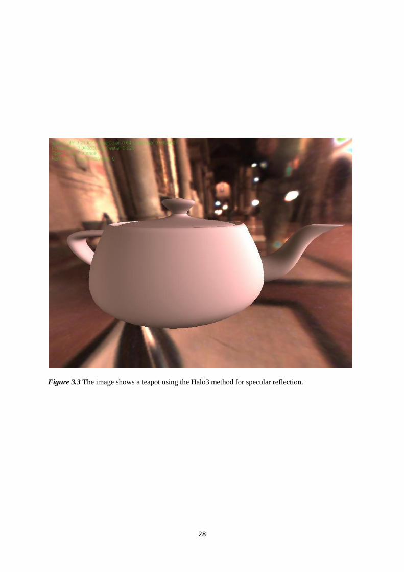
texture was small in size, the space was not a problem. Figures 3.3 and 3.4 show the results of
the combined Halo3-real Cook Torrance method. The method was used to lighten a teapot in
two different environments. As can be seen, the method captures low frequency reflections
but fails in terms of creating sharp reflections.
28
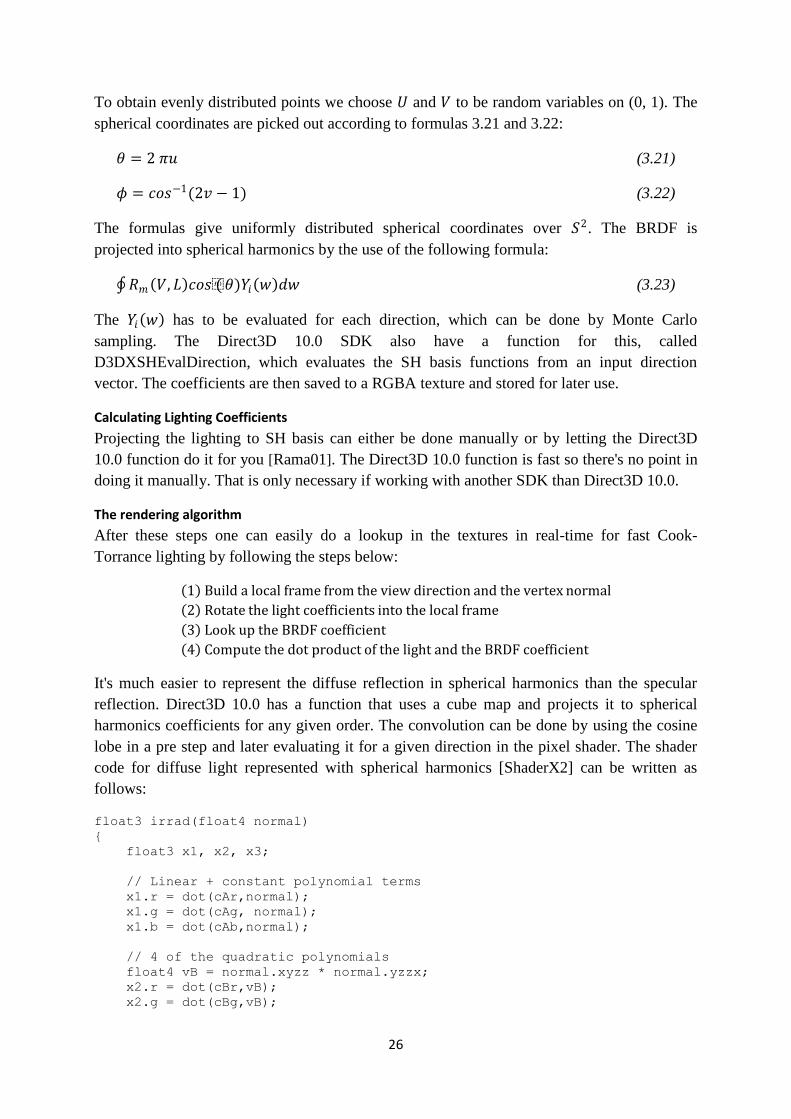
Figure 3.3 The image shows a teapot using the Halo3 method for specular reflection.
29
Figure 3.4 A teapot using the Halo3 method

30
Combining Halo3 method with skin rendering techniques
The Halo3 method can be used for any material and can also be combined with different skin
rendering techniques to optimize the result. The skin rendering methods, which were used for
this purpose in this project are subsurface scattering, Gaussian shadow mapping (with
integrated light positioning from the Median Cut Algorithm), and finally diffuse reflection
with spherical harmonics.
In figure 3.5 and 3.6 the Halo 3 method is compared to the Soho wavelets technique in two
different environments. The images are taken with a uniform gray texture and the diffuse
reflection derives from an environment map. As you can see, the high glossy reflection is
missing in image (c), which is the result of the Halo3 method. This is due to the fact, that the
Halo3 method can only represent low frequencies and therefore lack of sharp reflections.
Moreover the reflection is smooth and widespread, which does not look realistic. On the other
hand the Halo3 technique is an order of magnitude faster than the Soho wavelet method.
Figure 3.5 The first image (a) is the Cook-Torrance model, the second image (b) is the
Kelemen/Szirmay-Kalos model and the last image (c) is the Cook-Torrance model represented with
the Halo3 method. The images are available in a larger size in appendices 12-14.
Figure 3.6 The images are based on the same methods as in figure 3.4, but the environment map
differs.
Figures 3.7-3.9 show results of the Halo3 method implemented in three different
environments. As can be seen from those images, it's difficult to represent both low specular
and glossy specular reflection at the same time. When scaling the reflection too much, it turns
out like a white diffuse reflection instead of a specular reflection, and also, the object appears
to output more energy than it receives. Images in figures 3.7 and 3.8 reflect light correctly
from grazing angles, whereas no strong reflection appears when light derives from above in
figure 3.9.

31
Figure 3.7 The image shows how the Halo3 method catches reflection at grazing angles.

32
Figure 3.8 The image shows how the Halo3 method catches reflection from above.

33
Figure 3.9 The image shows how the Halo3 method catches reflection at grazing angles.

34
3.2.3 Conclusions
Representing the Cook Torrance BRDF model in spherical harmonics is an efficient and a low
storage technique for environment lighting. Normally when working with complex BRDF,
such as the Cook-Torrance model, different storages are needed for each material if the
calculation hasn't been accomplished in the shader. With the Halo3 method, it's possible to
represent different roughness parameters of the materials, with a small 2D texture, and also,
the calculations can be performed during the pre-process. Furthermore, separation of the
reflection into different layers is a good approximation for all frequency reflection, but it is
only the lowest reflections that can be represented in a correct way. To be able to capture both
low and high frequencies , we need other bases than spherical harmonics.
The Halo3 method shows good results in some environments and angles, but for the most, it
must be combined with high frequency reflection represented with point lights, in order to
generate high quality reflections.
3.3 Wavelets What we concluded from the previous chapter, is that spherical harmonics are good for
representing low frequency light but not for high frequency. Wavelets, which are other bases
for representing environment lighting, can capture both low and high frequency light in a
compact manner. A good thing about them is that their basis can contain functions of different
sizes and positions. Some waves are small and as a result they can represent just a pixel, while
other waves are bigger, i.e. they can capture light from the whole environment.
This part of the thesis treats the implementation of wavelets, with an objective to be able to
represent specular reflection for dynamic objects with both high and low frequencies from
environment lighting.
3.3.1 Theory
Wavelets have been studied for over 25 years, but there is still no clear definition of what they
are. However, the main advantages of wavelets compared to other basis have been identified
[Soho08, Primer1]:
1. Localization in space or time: The special attributes of wavelets are that they are
localized in both space and frequency while the standard Fourier transform is only
localized in frequency. These attributes make them a powerful tool for representing
signals (like the lighting function). Furthermore wavelets can represent large changes
because they have local support; unlike Fourier or spherical harmonics which have
global support.
2. Fast transform algorithm: Transformation of wavelets are faster than Fourier basis, as
they take 𝑂(𝑁) compared to 𝑂(𝑁 𝑙𝑜𝑔 𝑁).
3. Arbitrary domains: Most bases can only represent functions defined in the Euclidean
space. Wavelets can be defined in 𝑋 ⊂ 𝑅𝑛 .
Wavelets are divided into two parts; the prototype function, which is called the mother
wavelet, and the scaled and translated wavelets, which are described as baby wavelets

35
[Primer1]. Furthermore, wavelets can be categorized into discrete and continuous wavelet
transformations. For compact representation and for approximation, the discrete wavelets are
preferable to use, whereas the continuous wavelets are more fit for analysis. For our
application, we use discrete wavelets [Soho08].
The goal of working with wavelets is to represent a lot information with as few coefficients as
possible. The wavelet is looking for local dissimilarity. Regions that are similar to the
coefficients are close to zero, whereas inhomogeneous regions have larger basis functions. It's
possible to discard all coefficients that are small and still get a good approximation of the
original signal. The discarding of small coefficient is called non-linear approximation.
[RenRavPat03, RenRavPat04].
By using wavelets we can represent an environment map with only a few wavelet coefficients.
Some coefficients represent just a pixel in the environment, while others represent frequencies
over the whole surrounding. Even though we discard a big amount of coefficients, the error is
insignificantly small [RenRavPat03, RenRavPat04].
The wavelet basis is a set of functions that are defined by a recursive difference equation:
𝜙 𝑥 = 𝑐𝑘𝜙 2𝑥 − 𝑘 𝑀−1𝑘=0 (3.24)
The wavelet equation is orthogonal to its translation; 𝜙 𝑥 𝜙 𝑥 − 𝑘 𝑑𝑥 = 0. and it is also
orthogonal to its dilation; 𝜓 𝑥 𝜓 𝑥 − 𝑘 𝑑𝑥 = 0.
The function 𝜓 is:
𝜓 𝑥 = −1 𝑘𝑐1−𝑘𝑘 𝜙 2𝑥 − 𝑘 (3.25)
The Haar Wavelet
The scaling basis for the Haar Wavelet is:
𝜙𝑖𝑗 𝑥 ≔ 𝜙 2𝑗𝑥 − 𝑖 , 𝑖 = 0,1,… 2𝑗 − 1 (3.26)
𝜙 𝑥 ≔ 1 𝑓𝑜𝑟 0 ≤ 𝑥 < 10 otherwise
(3.27)
The wavelet basis for the Haar Wavelet can be described as:
𝜓𝑖𝑗 𝑥 ≔ 𝜓 2𝑗𝑥 − 𝑖 , 𝑖 = 0,1,… , 2𝑗 − 1 (3.28)
𝜓 𝑥 ≔ 1 𝑓𝑜𝑟 0 ≤ 𝑥 < 1/2 −1 𝑓𝑜𝑟 1/2 ≤ 𝑥 < 1
0 otherwise
(3.29)
The Haar basis has an important property known as orthogonality, which means that the
functions ϕ00, ψ
00, ψ
01 , ψ
11 are orthogonal to each other. The formulas 3.26-3.27 are orthogonal
but not orthonormal. The basis can be normalized by calculating the magnitude of each of
these vectors and then dividing their components by that magnitude. The Haar basis can then
be described as [Primer1]:

36
𝜙𝑖𝑗≔ 2
𝑗
2 𝜙 2𝑗𝑥 − 𝑖 (3.30)
𝜓𝑖𝑗 𝑥 ≔ 2
𝑗
2 𝜓 2𝑗𝑥 − 𝑖 (3.31)
The constant factor 2j
2 is chosen so that u| u = 1 for the standard inner product.
Figure 3.10 illustrates the first four scaling bases and the wavelet bases.
Source: [Primer1]
Figure 3.10 The top images demonstrate the first four scaling basis. The wavelet bases are illustrated
at the bottom of the image.

37
Projecting the Haar wavelet
There are two kind of bases; linear and non-linear. When projecting a function to a linear
basis the same static basis is used at all times. When projecting a function to a non-linear
basis, such as the Haar wavelet, a dynamic set of bases functions are used to represent the
function in the most optimal way. To understand how the projecting of a function into Haar
wavelet works, an example by Musawir Ali is presented [HAAR2D]:
We start the example by creating four Haar wavelet bases. After choosing a basis vector
1, 1, 1, 1 , we need to find three more bases that are orthogonal to the first vector. For
example we can use; 1, 1,−1,−1 , 1,−1, 0, 0 and 0, 0, 1,−1 . These four vectors are
perpendicular to each other, however they are not orthonormal and therefore they do not fit
the requirements of many applications. To make the vectors orthonormal, they should be
divided by the magnitude of the vector. The first four Haar bases are both orthogonal and
orthonormal:
1/2, 1/2, 1/2, 1/2
1/2, 1/2,−1/2,−1/2
1/ 2,−1/ 2, 0, 0
0, 0, 1/ 2,−1/ 2
We can now project a vector into the Haar basis functions. This can be done by simply
calculating the dot product of the input vector and each of the basis vectors. The input vector
is 4,2,5,5 . Accordingly the projection can be described as:
4, 2, 5, 5 ∙ 1/2, 1/2, 1/2, 1/2 = 8
4, 2, 5, 5 ∙ 1/2, 1/2,−1/2,−1/2 = −2
4, 2, 5, 5 ∙ 1/ 2,−1/ 2, 0, 0 = 2/ 2
4, 2, 5, 5 ∙ 0, 0, 1/ 2,−1/ 2 = 0
The input vector is now transformed into 8,−2, 2/ 2, 0 . The forth component is zero and it
is possible to discard it. Consequently the original vector is now represented by three
components instead of four. This is done without the loss of any information. To recover the
original vector, the transformed vector is multiplied with the Haar bases and the result is
summarized in order to obtain the original vector 4,2,5,5 :
8 ∗ 1/2, 1/2, 1/2, 1/2 = 4, 4, 4, 4
−2 ∗ 1/2, 1/2,−1/2,−1/2 = −1,−1, 1, 1
2/ 2 ∗ 1/ 2,−1/ 2, 0, 0 = 1,−1, 0, 0

38
The Haar 2D matrix transformation algorithm
The Haar 2D algorithm that transforms an input matrix to Haar wavelets.
𝑨𝒍𝒈𝒐𝒓𝒕𝒊𝒉𝒎:𝐻𝑎𝑎𝑟 2𝐷 𝑑𝑒𝑐𝑜𝑚𝑝𝑜𝑠𝑖𝑡𝑖𝑜𝑛
𝑰𝒏𝒑𝒖𝒕: 𝐴 𝑛 𝑥 𝑛 𝑖𝑚𝑎𝑔𝑒: 𝑖𝑚𝑔,𝑛𝑢𝑚𝑏𝑒𝑟 𝑜𝑓 𝑠𝑡𝑒𝑝:𝑛𝑠𝑡𝑒𝑝𝑠
𝑶𝒖𝒕𝒑𝒖𝒕:𝐻𝑎𝑎𝑟 2𝐷 𝑤𝑎𝑣𝑒𝑙𝑒𝑡𝑠 𝑐𝑜𝑒𝑓𝑓𝑖𝑐𝑖𝑒𝑛𝑡
1 ← 𝑛
2 𝑠𝑡𝑒𝑝 ← 0
3 𝑤𝑖𝑙𝑒 > 1 𝑎𝑛𝑑 𝑛𝑠𝑡𝑒𝑝𝑠 = 0 𝑜𝑟 𝑠𝑡𝑒𝑝 < 𝑛𝑠𝑡𝑒𝑝
4 𝑎𝑎𝑟2𝐷𝐷𝑒𝑐𝑜𝑚𝑝𝑋 𝑖𝑚𝑔, ,𝑛
5 𝑎𝑎𝑟2𝐷𝐷𝑒𝑐𝑜𝑚𝑝𝑌 𝑖𝑚𝑔, ,𝑛
6 ←
2
7 𝑠𝑡𝑒𝑝 ← 𝑠𝑡𝑒𝑝 + 1
8 𝑟𝑒𝑡𝑢𝑟𝑛 𝑖𝑚𝑔
𝑨𝒍𝒈𝒐𝒓𝒕𝒊𝒉𝒎: 𝑎𝑎𝑟2𝐷𝐷𝑒𝑐𝑜𝑚𝑝𝑋
𝑃𝑒𝑟𝑓𝑜𝑟𝑚𝑠 𝑜𝑛𝑒 𝑠𝑡𝑒𝑝 𝑜𝑓 𝑤𝑎𝑣𝑒𝑙𝑒𝑡 𝑑𝑒𝑐𝑜𝑚𝑝𝑜𝑠𝑖𝑡𝑖𝑜𝑛 𝑖𝑛 𝑡𝑒 𝑥 − 𝑑𝑖𝑚𝑒𝑛𝑠𝑖𝑜𝑛
1 2 ←
2
2 𝑦𝑛𝑑𝑥 ← 0
3 𝑓𝑜𝑟 𝑖 ← 0 𝑡𝑜 − 1
4 𝑦𝑛𝑑𝑥 ← 𝑦𝑛𝑑𝑥 + 𝑛
5 𝑓𝑜𝑟 𝑗 ← 0 𝑡𝑜 2
6 𝑛𝑑𝑥1 ← 𝑦𝑛𝑑𝑥 + 𝑗
8 𝑛𝑑𝑥2 ← 𝑦𝑛𝑑𝑥 + 2 + 𝑗
9 𝑛𝑑𝑥3 ← 𝑦𝑛𝑑𝑥 + 2 ∗ 𝑗
10 𝑛𝑑𝑥4 ← 𝑦𝑛𝑑𝑥 + 2 ∗ 𝑗 + 1
11 𝑡𝑒𝑚𝑝 𝑛𝑑𝑥1 ← 𝑖𝑚𝑔 𝑛𝑑𝑥3 + 𝑖𝑚𝑔 𝑛𝑑𝑥4 ∗1
2
12 𝑡𝑒𝑚𝑝 𝑛𝑑𝑥2 ← 𝑖𝑚𝑔 𝑛𝑑𝑥3 − 𝑖𝑚𝑔 𝑛𝑑𝑥4 ∗1
2
13 𝑠𝑤𝑎𝑝(𝑖𝑚𝑔, 𝑡𝑒𝑚𝑝)
𝑨𝒍𝒈𝒐𝒓𝒕𝒊𝒉𝒎: 𝑎𝑎𝑟2𝐷𝐷𝑒𝑐𝑜𝑚𝑝𝑌
𝑃𝑒𝑟𝑓𝑜𝑟𝑚𝑠 𝑜𝑛𝑒 𝑠𝑡𝑒𝑝 𝑜𝑓 𝑤𝑎𝑣𝑒𝑙𝑒𝑡 𝑑𝑒𝑐𝑜𝑚𝑝𝑜𝑠𝑖𝑡𝑖𝑜𝑛 𝑖𝑛 𝑡𝑒 𝑦 − 𝑑𝑖𝑚𝑒𝑛𝑠𝑖𝑜𝑛
1 2 ←
2
2 𝑦𝑛𝑑𝑥 ← 0
3 𝑓𝑜𝑟 𝑖 ← 0 𝑡𝑜 − 1
4 𝑦𝑛𝑑𝑥 ← 𝑦𝑛𝑑𝑥 + 𝑛
5 𝑓𝑜𝑟 𝑗 ← 0 𝑡𝑜 2
6 𝑛𝑑𝑥1 ← 𝑦𝑛𝑑𝑥 + 𝑖
8 𝑛𝑑𝑥2 ← 𝑦𝑛𝑑𝑥 + 2 ∗ 𝑛 + 𝑖
9 𝑛𝑑𝑥3 ← 𝑦𝑛𝑑𝑥 ∗ 2 + 𝑖
10 𝑛𝑑𝑥4 ← 𝑦𝑛𝑑𝑥 ∗ 2 + 𝑛
11 𝑡𝑒𝑚𝑝 𝑛𝑑𝑥1 ← 𝑖𝑚𝑔 𝑛𝑑𝑥3 + 𝑖𝑚𝑔 𝑛𝑑𝑥4 ∗1
2
12 𝑡𝑒𝑚𝑝 𝑛𝑑𝑥2 ← 𝑖𝑚𝑔 𝑛𝑑𝑥3 − 𝑖𝑚𝑔 𝑛𝑑𝑥4 ∗1
2
13 𝑠𝑤𝑎𝑝(𝑖𝑚𝑔, 𝑡𝑒𝑚𝑝)

39
Soho wavelets
The Haar wavelet lies in the planar domain and leads to distortion when used for functions in
other domains. Christian Leesig, author of "The Soho Wavelets", proposes a new kind of
wavelet, that is called the Soho wavelet, which can be described as an orthogonal and
symmetric Haar wavelet. The Soho wavelet is a second generation wavelet and gives less
distortion than the basic Haar 2D [Soho08]. Many applications in computer graphics and
physics require the rotation of signals. Therefore Leesig has developed a way to analytically
build a rotation matrix for the Soho wavelets. The bases functions of the Soho wavelet are
described below.
Scaling basis functions
𝜑𝑗 ,𝑘 = 𝑗 ,𝑘 ,𝑙𝜑𝑗 ,𝑘𝑙4
𝑙=1 (3.32)
Wavelet basis functions
𝜓𝑗 ,𝑘𝑖 = 𝑔𝑗 ,𝑘 ,𝑙
𝑖 𝜑𝑗 ,𝑘𝑙4
𝑙=1 (3.33)
The Soho wavelets are defined over a partition 𝑇 that is characterized by a set of spherical
triangles 𝑇 = 𝑇𝑗 ,𝑘 |𝑗 ∈ 𝐽,𝑘 ∈ 𝐾 (𝑗) . The domain at the coarsest level 𝑇0,𝑘 are obtained by
projecting a platonic solid with triangular faces such as the octahedron onto the sphere (figure
3.11).
Source: [Soho08].
Figure 3.11 The first two images from the left show how an octahedron is projected onto a sphere.
The last two images show how the spherical triangles are subdivided from the coarsest to a fine level.
The domains at finer level are formed by recursively subdividing every spherical triangle Tj,k
into four new triangles Tj+1,lk . These are obtained by inserting one new vertex vj,k
l on each of
the arcs forming the sides of the Tj,k . All triangles that are created from the octahedron can be
seen as a partition tree with the octahedron triangles as the root nods. To be able to keep
orthogonal and symmetric Soho bases it's required that the three outer spherical triangles have
equal areas. In other words: Tj+1,1k = Tj+1,2
k = Tj+1,3k .

40
Source: [Soho08]
Figure 3.12 The figure demonstrates a spherical triangle to the left and to the right a triangle, divided
into four sub-triangles, in which the outer triangles have the same area.
Spherical triangle
A spherical triangle is a triangle formed on the surface of a sphere by three circular arcs
intersecting pair wise in three vertices. A spherical triangle (figure 3.12) is specified by its
corner angles and its sides, which are given by their arc angles. The angles in a spherical
triangle is always larger then 180∘. The amount E by which the sum of angles exceeds 180∘
is called spherical excess and is used to calculate the area [STWolf]. If R is the radius of the
sphere and α,β and γ are the angles, the formula for the area is:
𝐸 = 𝛼 + 𝛽 + 𝛾 − 𝜋 (3.34)
𝐴 = 𝑅2𝐸 (3.35)
Stratified Monte Carlo sampling for spherical triangles
Picking uniformly distributed random samples from arbitrary spherical triangles is not easy.
There are many different sampling algorithms for various geometries, but few methods exist
for sampling solid angles; that is, for regions on the unit sphere. James Arvo has presented a
stratified algorithm that show good results for this purpose [Arvo95]. James algorithm can be
formulated using elementary spherical trigonometry.
Source: [Arvo95]
Figure 3.13 The image shows how a sample point P is chosen from an arc between two vertices.

41
In figure 3.13, A, B and C are the vertices of the triangle and a, b and c denotes the length of
each arc. The angle between each arc is symbolized by α,β and γ. The algorithm creates a
new subtriangle by choosing a new vertex A on the edge between A and C. The sample point
is then chosen on the arc between vertex A and B. The point P is dependent of the distance d
from B and the length of b . Accordingly, a sample point P is chosen from an arc between two
vertices as shown in figure 3.13. The values are computed using the conditional distribution
functions [Arvo05].
3.3.2 Implementation and results
Wavelets are representative for both low and high frequency light in a compact way. The
wavelet implementation part of this project can be divided in to two parts, the first part
includes implementation of the Haar 2D wavelet combined with self occlusion, and the
second part involves implementation of Soho wavelets and an approximation method used for
rotation of the object and in order to achieve a dynamic view. As part of the Haar wavelet
implementation, diffuse light is represented by an environment map and the object is static.
The Soho wavelets are represented by both diffuse and specular reflection, including a static
view direction.
Haar wavelet occlusion
The most popular way to calculate occlusion is to ray trace light in different directions from
an objects vertex. Ray tracing involves tracing the path of light through pixels in an image
plane. A light ray increases the brightness of the vertex while a ray that hits an object does not
contribute to any illumination. Ray tracing is one of the most accurate methods for self
occlusion but a good ray tracer can be quite complicated to program. One of the problems is
that the PRT step will increase in time as the number of rays increase. To avoid this problem
it's possible to draw a hemi cube from each vertex on the object and store it in an environment
map. This method will proceed faster than a ray tracer since it can be implemented on the
GPU. Furthermore all 6 texture in a cube map can be calculated in just one draw, by using the
geometry shader.
Algorithm: the pre process step for wawelet occlusion
1 for each vertex
2 draw a visibility cube map and multiply it with a cosine weight
3 transform the cube map to wavelets and store it in a transport matrix
4 convert the light to wavelets and apply non − linear approximation to it
5 save the coefficient to disc
Algorithm: the wavelet occlusion rendering algorithm
1 for each vertex
2 multiply the light wavelets with the vertex occlusion wavelets
using sparse matrix multiplication
The first implementation with wavelets included the Haar 2D wavelets with self occlusion. In
order to make self occlusion accessible, a sphere like object in Maya was created. As can be
seen in figure 3.14, there are soft shadows around the rectangles reaching out from the sphere.

42
The pre-process is time consuming but the rendering process proceeds quickly, since the
computing for diffuse reflection is finished before and also no shadows maps are needed.
Figure 3.14 The image shows an occluded object that was produced with Haar 2D wavelets.
Soho wavelets
The Soho wavelet is both orthogonal and symmetric and is well suited for representation of
functions on the sphere such as the light equation. Implementing the Soho wavelets includes
building of a partition tree with spherical triangles, which is quite complicated to apply. When
dividing a spherical triangle in to four sub triangles, the three outer triangles must have the
same area in order to maintain the orthogonality of the Soho bases. The equations for
constructing the subdivisions are time-consuming and difficult to write. Accordingly Matlab
implementations on Soho wavelets by Christian Lessig were translated into C++ and then
optimized. The algorithm, that can be utilized when creating the Soho wavelets and building
the partition tree can be written in following way:
𝐀𝐥𝐠𝐨𝐫𝐢𝐭𝐡𝐦: The Soho wavelet algorithm
1 create and octahedron inside a unit sphere,
this will create 8 spherical triangles
2 for each triangle
3 recursive subdivide it to the desired level
4 Sample the signal light onto the domains of the finest
level of the partition tree
5 Tranform the signal at the finest level into Soho wavelets
6 Discard non zero coefficient
Even though the Soho wavelets resulted in more details and less artifacts than the Haar 2D
wavelet, there are problems left in terms of representing specular reflection with a viewing

43
camera and a rotated object. If we want to represent the specular reflection, which is view
dependent, the transportation matrix becomes gigantic and we will not be able to rotate the
object. Christian Lessig has developed a method to rotate the Soho wavelets. If we were able
to rotate the signal we could use the same idea as for the Halo3 implementation, that is,
rotating the light into the local frame. The conclusions of the research in the area of how the
rotation matrix was created, revealed that it was too complicated and time consuming to use
the Leesig rotation method for rotation of the light in a real time game. The rotation matrix
was too large and the rotation of the signal for each vertex was not achievable.
The Soho wavelets are located in both frequency and space and the coefficients are located on
the sphere. Each sub triangle on the finest level of the partition has also a location in world
space, which easily can be calculated. If the partition tree is sub divided into many step, the
spherical triangles become very small. As a result, the distance between two adjacent sub
triangles' world positions is insignificant and thus the sub triangles can be approximated to the
same world position. If the coefficients with the largest terms are identified, it is possible to
calculate the BRDF for the same directions in the pixel shaders, transform it to Soho wavelet
and then multiply it with the lighting coefficient. This way the object can be rotated, the view
direction changed and a specular reflection obtained. The cost of the algorithm depends on the
number of coefficients chosen from the light wavelets. What's more, the cost also dues to how
complicated the BRDF is; the more complicated the BRDF is, the less wavelet coefficients
can be used for rendering purposes. The number of coefficients must be the same as the
number of BRDF:s. Furthermore they must be calculated in the shader.
𝐀𝐥𝐠𝐨𝐫𝐢𝐭𝐡𝐦: Soho approximation algorithm
1 Create the Soho wavelets for the light
2 Sort the coefficients at the finest level and calculate their world position
3 Send the 𝑛 largest coefficient with its position to the to GPU This is done in a pre
− process
4 Calculate the BRDF for 𝑛 position and tranform it to Soho wavelets
5 Multiply the light and the BRDFs wavelets to get the final color
The Soho approximation method, was tested it in three different environments (light probes),
and variable quantities of wavelets coefficient. The light probes are taken from Paul
Debevec's Light Probe Gallery [Probes]. The first one is the Galileo's Tomb at Santa Croce
with a dynamic range of 7000:1; the second probe is The Uffizi Gallery and has a dynamic
range of 500:1 and the last probe is the St. Peter's Basilica in Rome with a dynamic range of
200,000:1. The number of coefficients that were used are 16, 32, 64, 256, 512. The 256 and
512 coefficients are too slow to work in a real time game but make good use as references,
since the result should look like them. Figures 3.15-3.20 show both specular reflection and
diffuse and specular reflection combined. Cook-Torrance was used in the implementation as
BRDF. Figures 3.21 and 3.22 show teapots with low roughness value and as can be seen, the
Soho wavelet captures sharp reflections from the whole environment.
44
Figure 3.15 Galileo's Tomb, diffuse light + specular reflection.
Figure 3.16 Galileo's Tomb, specular reflection. Enlarged images are available in appendices 15-19.

45
Figure 3.17 St. Peter's Basilica, diffuse + specular light.
Figure 3.18 St. Peter's Basilica, specular reflection.
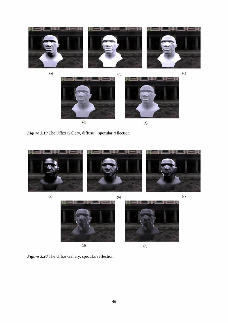
46
Figure 3.19 The Uffizi Gallery, diffuse + specular reflection.
Figure 3.20 The Uffizi Gallery, specular reflection.

47
Figure 3.21 The Uffizi Gallery, specular reflection.

48
Figure 3.22 The Uffizi Gallery, specular reflection.
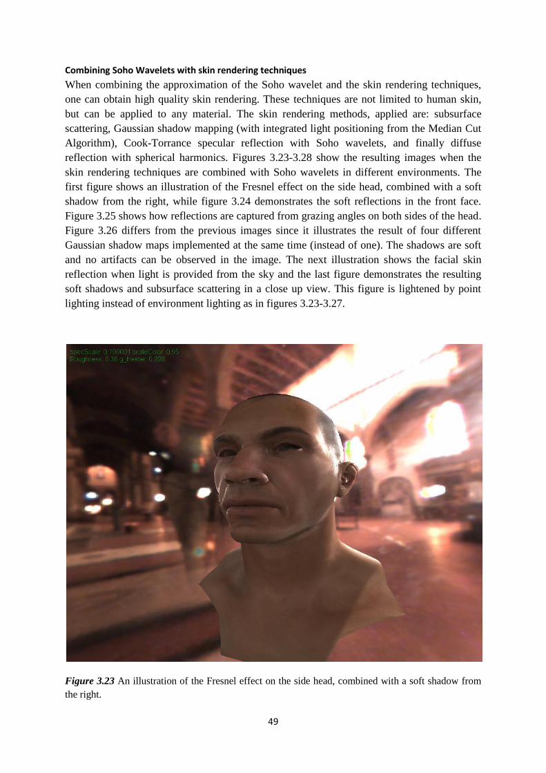
49
Combining Soho Wavelets with skin rendering techniques
When combining the approximation of the Soho wavelet and the skin rendering techniques,
one can obtain high quality skin rendering. These techniques are not limited to human skin,
but can be applied to any material. The skin rendering methods, applied are: subsurface
scattering, Gaussian shadow mapping (with integrated light positioning from the Median Cut
Algorithm), Cook-Torrance specular reflection with Soho wavelets, and finally diffuse
reflection with spherical harmonics. Figures 3.23-3.28 show the resulting images when the
skin rendering techniques are combined with Soho wavelets in different environments. The
first figure shows an illustration of the Fresnel effect on the side head, combined with a soft
shadow from the right, while figure 3.24 demonstrates the soft reflections in the front face.
Figure 3.25 shows how reflections are captured from grazing angles on both sides of the head.
Figure 3.26 differs from the previous images since it illustrates the result of four different
Gaussian shadow maps implemented at the same time (instead of one). The shadows are soft
and no artifacts can be observed in the image. The next illustration shows the facial skin
reflection when light is provided from the sky and the last figure demonstrates the resulting
soft shadows and subsurface scattering in a close up view. This figure is lightened by point
lighting instead of environment lighting as in figures 3.23-3.27.
Figure 3.23 An illustration of the Fresnel effect on the side head, combined with a soft shadow from
the right.

50
Figure 3.24 The figure demonstrates the soft reflections in the front face, accomplished by combining,
skin rendering techniques and wavelet bases.
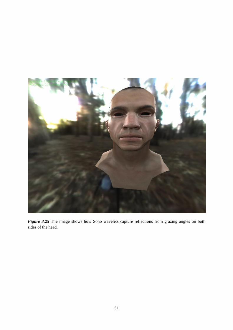
51
Figure 3.25 The image shows how Soho wavelets capture reflections from grazing angles on both
sides of the head.

52
Figure 3.26 The figure shows the result of four different Gaussian shadow maps implemented at the
same time. The shadows are soft and no artifacts can be observed.

53
Figure 3.27 An illustration of the facial skin reflection when light is provided from the sky.

54
Figure 3.28 Another illustration of subsurface scattering and soft shadows in a close up view.

55
3.3.3 Conclusions
One of the objectives of wavelet implementation, was to be able to represent specular
reflection for dynamic objects with both high and low frequencies. The first implementations
combined self occlusion and diffuse reflection with the Haar 2D wavelets. Only diffuse
reflection could be represented and furthermore the application was based on static objects,
which of course is inapplicable in games. The self occluded shadows were soft and looked
natural, but since this wasn't the real purpose of the implementation, it was a failure.
The Soho wavelets are represented on the sphere instead of the plane and accordingly, it gave
better results. The approximation method for the Soho wavelets is quite expensive, but on the
other hand, it can be run in real-time with the light coming from a whole environment map.
Furthermore the reflection is represented with a complicated BRDF, which results in more
realistic materials. Figures 3.15-3.20 illustrate that the Soho wavelets are good at capturing
both low and high frequency reflections. However, as can be seen in the figures, low
frequencies are missing out when using too few coefficients.
The research of representing irradiance with wavelets is just in the beginner phase and as a
conclusion these types of applications are not ready to be used in real time games. However
the future looks promising for the wavelet bases.

56
4. Evaluation of the results The results of the subsurface scattering techniques were much better than expected. Human
faces in modern computer games look harsh and plastic and the techniques presented in this
report will generate more realistic outcomes. The implemented subsurface scattering
technique gives a soft appearance and makes the red color scatter further than the green and
blue colors. Also, subsurface scattering solves the problems with harsh self shadowing. Often,
the shadows in modern games have big artifacts and look unreal. When combing subsurface
scattering with Gaussian filters for shadow mapping some of these artifacts are eliminated. As
presented in this report, the shadows look soft and smooth with this combined technique, even
when the camera is close to the object. The results imply that it is possible to render realistic
human skin in real time at a low cost.
The other part of the project was to investigate the specular reflection from environment
lighting. One option is to representing specular reflection with spherical harmonics and the
Halo3 technique. Spherical harmonics basis are fast but their limitation to only represent low
frequencies makes them unfit for future rendering. What we need are new basis that are fast
and can represent both low and high frequencies. As a conclusion the Halo3 technique does
not generate particularly good results for specular reflection. At the same time one must have
in mind that it is preferable to the current techniques, which are limited to point lighting. By
using the Halo3 method, the same pre-computed textures can be used for all kinds of material,
and the BRDF is not limited to its calculation time as in point lighting.
Wavelets are other basis that puts spherical harmonics in the shade in terms of visual
appearance. Even with few coefficients amazing results can be obtained. Soho wavelets are
built in such a way that they can be approximated in order to be used for rotating objects.
They are quite costly but can be used for any material and what's more, the pre-computations
only has to be performed once. When looking back at the teapot in figure 3.21, we can certify
that Soho wavelets capture a lot of high frequencies and that the teapot reflects specular light
from different areas of the environment map. This is something that could never be done with
spherical harmonics. When wavelets are combined with skin rendering techniques, a high-
quality method is established for rending complex materials from environment light, with
both diffuse and specular reflection represented in a physically correct way.
The aim of this project was to establish more advanced real-time rendering techniques for
complex materials such as human skin. The new techniques presented in this report can solve
some of the problems that appear when trying to lighten material in a physically correct way
and in real time.
The results of this thesis imply that it is possible to render realistic human skin in real time at
a low cost. When Wavelets are combined with skin rendering techniques, a high-quality
method is established for rending complex materials from environment light, with both
diffuse and specular reflection represented in a physically correct way.

57
5. Glossary Blinn-Phong model
BRDF
BSSRDF
Cook-Torrance method
Diffuse profile
Diffuse reflection
EA
Haar wavelet
Halo3 method
Fresnel effect
Kelemen/Szirmay-Kalos
Median Cut Algorithm
Soho wavelet
PCF
Specular reflection
a simple BRDF.
(Bidirectional Reflectance Distribution Function) the
normal BRDF is an approximation of the BSSRDF and
defines how light is reflected at an opaque surface.
(Bidirectional Surface Scattering Reflectance
Distribution Function): used to name the general
mathematical function which describes the way in which
the light is scattered by a surface.
a specular-microfacet model accounting for color
shifting, a BRDF.
the diffuse profile demonstrates how light scatters across
a radial distance from its hit point and tells us how much
light emerges as a function of the angle and distance
from the laser center.
the reflection of light from an uneven surface such that
an incident ray is seemingly reflected at a number of
angles. It is the complement to specular reflection.
Electronic Arts, an international developer, marketer,
publisher and distributor of video games.
the simplest possible wavelet, which lies in the planar
domain.
a new method with spherical harmonics used in this
thesis.
effect of the Fresnel equation, which describes the
behavior of light when moving between media of
differing refractive indices.
a BRDF.
a popular algorithm for color quantization.
a second generation wavelet.
percentage closer filtering; to take a number of samples
around the shaded fragment and compute the average.
the mirror-like reflection of light from a surface, in
which light from a single incoming direction is reflected
into a single outgoing direction.

58
Spherical Harmonics
SSS
Subsurface scattering
Translucent shadow map
TSM
Wavelet
the angular portion of a set of solutions to Laplace's
equation. In 3D computer graphics, spherical harmonics
plays a special role in indirect lighting and recognition of
3D shapes.
subsurface scattering.
a mechanism of light transport in which light penetrates
the surface of a translucent object, is scattered by
interacting with the material, and exits the surface at a
different point.
an extension to shadow maps which allows very efficient
rendering of sub-surface scattering.
translucent shadow maps.
a mathematical function used to divide a given function
or continuous-time signal into different scale
components.

59
References [ATI04] J. Isidoro, C. Oat, J. Mitchell “Next Generation Skin Rendering” 2004
[Borshukov03] G. Borshukov and J. P. Lewis. “Realistic Human Face Rendering for The Matrix Reloaded,” in
ACM SIGGRAPH Sketches and Applications, 2003.
[Borshukov05] G. Borshukov and J. P. Lewis. “Fast Subsurface Scattering” in ACM SIGGRAPH 2005 Course
on Digital Face Cloning, 2005.
[d'EonGDC07] E. d'Eon, “NVIDIA Demo Team Secrets-Advanced Skin Rendering,” available online at
http://developer.download.nvidia.com/presentations/2007/gdc/Advanced_Skin.pdf.
[d'EonEuro07] E. d'Eon, D. Luebke, E. Enderton, “Efficient Rendering of Human Skin,” in Rendering
Techniques 2007 (Proceedings of the Eurographics Symposium on Rendering), Grenoble, France.
[d'EonGPU07] E. d'Eon, D. Luebke, “Advanced Techniques for Realistic Real-Time Skin Rendering,” in GPU
Gems 3, pp. 293-348, 2007.
[Donner05] C. Donner, H. Wann Jensen, “Light Diffusion in Multi-Layered Translucent Materials,” in ACM
Transactions on Graphics (Proceedings of SIGGRAPH 2005), 24(3).
[Green04] S. Green, “Real-Time Approximations to Subsurface Scattering,” in GPU Gems, edited by Randima
Fernando, pp.263-278. Addison-Wesley.
[Gritz07] L. Gritz and E. d'Eon, “The Importance of Being Linear,” in GPU Gems 3, edited by Hubert Nguyen,
pp. 529-542, 2007.
[Kelemen01] C. Kelemen and L. Szirmay-Kalos, “A Microfacet Based Coubled Specular-Matte BRDF Model
with Importance Sampling,” presented at Eurographics, 2001.
[NVIDIA06] NVIDIA Corporation, “Adrianne”, http://www.nzone.com/object/nzone_adrianne_home.html,
2006.
[NVIDIA07] NVIDIA Corporation, “Human Head”,
http://www.nzone.com/object/nzone_humanhead_home.html, 2007. (2009-05-18)
[Jensen01] H.W. Jensen, S.R.Marschner, M. Levoy, P. Hanrahan “A Practical Model for Subsurface Light
Transport”, , Proceedings of SIGGRAPH 2001.
[CookTo81] R. L. Cook, Torrance, K. E.. A reflectance model for computer graphics. In Proceedings of ACM
SIGGRAPH 1981, pp. 307–316.
[Schlick94] C. Schlick, An inexpensive BRDF model for physically-based rendering. Computer Graphics
Forums. 13, (3), 233–246. 1994
[GCD08] L. Bavoil, “Advanced Soft Shadow Mapping Techniques”, Game Developer Conference, 2008
[GDC09] The upcoming paper from the Game Developer Conference on advanced shadows, 2009
[Crow84] C. Franklin. “Summed-Area Tables for Texture Mapping” In Computer Graphics (Proceedings of
SIGGRAPH 1984) 18(3), pp. 207–212.
[RealTime] Tomas Akenine-Möller, Eric Haines, and Naty Hoffman, “Real-Time Rendering”, 2008
[Paul05] P. Debevec, A Median Cut Algorithm forLight Probe Sampling, 2005
[Probes] P. Debevec “Light Probe Image Gallery” http://www.debevec.org/Probes/ (2009-05-18)

60
[Olof07] O. Landahl, “Median Cut Algorithm in Image Based Lighting” TNM078 Image Based Rendering
Linköpings Universitet, 2007
[Green03] R. Green, “Spherical Harmonic Lighting: The Gritty Details”, 2003
[Halo08] H. Chen, X. Liu, “Lighting and Material of Halo3” Advances in real-time rendering in 3D Graphics
and Game Course SIGGRAP, 2008
[MCI] “Monte Carlo integration” http://mathworld.wolfram.com/MonteCarloIntegration.html (2009-05-18)
[SHPP] “Sphere Point Picking” http://mathworld.wolfram.com/SpherePointPicking.html (2009-05-18)
[SHWolf] “Spherical Harmoncis” http://mathworld.wolfram.com/SphericalHarmonic.html (2009-05-18)
[BasriJacobs03] R. Basri, D. W. Jacobs,. Lambertian reflectance and linear subspaces. IEEE Trans. Pattern Anal.
Mach. Intell. 25, 2, pp. 218–223, 2003
[KAUTZ02] J. Kautz, P. P. Sloan, J. Snyder. “Fast, arbitrary brdf shading for low-frequency lighting using
spherical harmonics”. In Proceedings of the 13th Eurographics workshop on Rendering 2002, pp. 291–296.
[Rama01] R. Ramamoorthi, P. Hanrahan, “An efficient representation for irradiance environment maps”,
Proceedings of ACM SIGGRAPH 2001, pp. 497–500.
[SLOANSNYDER02] J. Kautz, P. P. Sloan, J. Snyder. Precomputed radiance transfer for real-time rendering in
dynamic, low frequency lighting environments. ACM Trans. 2002 Graph. 21, 3, 527–536.
[ShaderX2] Peter-Pike J. Sloan, “ShaderX2: Shader Programming Tips and Tricks with DirectX 9.0” pp. 226 -
231
[Primer1] Eric J. Stollnitz, Tony D. DeRose, David H. Salesin “Wavelets for Computer Graphics: A Primer Part
1”
[Primer2] Eric J. Stollnitz, Tony D. DeRose, David H. Salesin , “Wavelets for Computer Graphics: A Primer”
[HAAR2D] Musawir Ali , “An Introduction to Wavelets and the Haar Transform” (2009-05-18)
[RenRavPat03] Ren Ng, Ravi Ramamoorthi, Pat Hanrahan 2003 “All-Frequency Shadows Using Non-linear
Wavelet Lighting Approximation”, ACM Transactions on Graphics, July 2003(Proceedings of SIGGRAPH)
[RenRavPat04] R. Ng, R. Ramamoorthi, P. Hanrahan, “Triple Product Wavelet Integrals for All-Frequency
Relighting”, ACM Transactions on Graphics, 2004
[RUI06] Rui Wang Ren Ng David Luebke Greg Humphreys, “Efficient Wavelet Rotation for Environment Map
Rendering”, Eurographics Symposium on Rendering (EGSR) 2006
[Soho08] Christian Lessig and Eugene Fium, “SOHO: Orthogonal and Symmetric Haar Wavelets on the
Sphere”, 2008
[STWolf] Spherical Triangle, http://mathworld.wolfram.com/SphericalTriangle.html, (2009-05-18)
[Arvo05] J. Arvo, “Stratified sampling of spherical triangles”, Proc. ACM Siggraph, August 1995.

61
Appendix
Appendix 1. Normal shadow map

62
Appendix 2. Shadow map with a 4x4 uniform filter

63
Appendix 3. Shadow map with a 5x5 Gaussian filter

64
Appendix 4. Diffuse light from St. Peter's Basilica, Rome

65
Appendix 5. Diffuse light with applied subsurface scattering
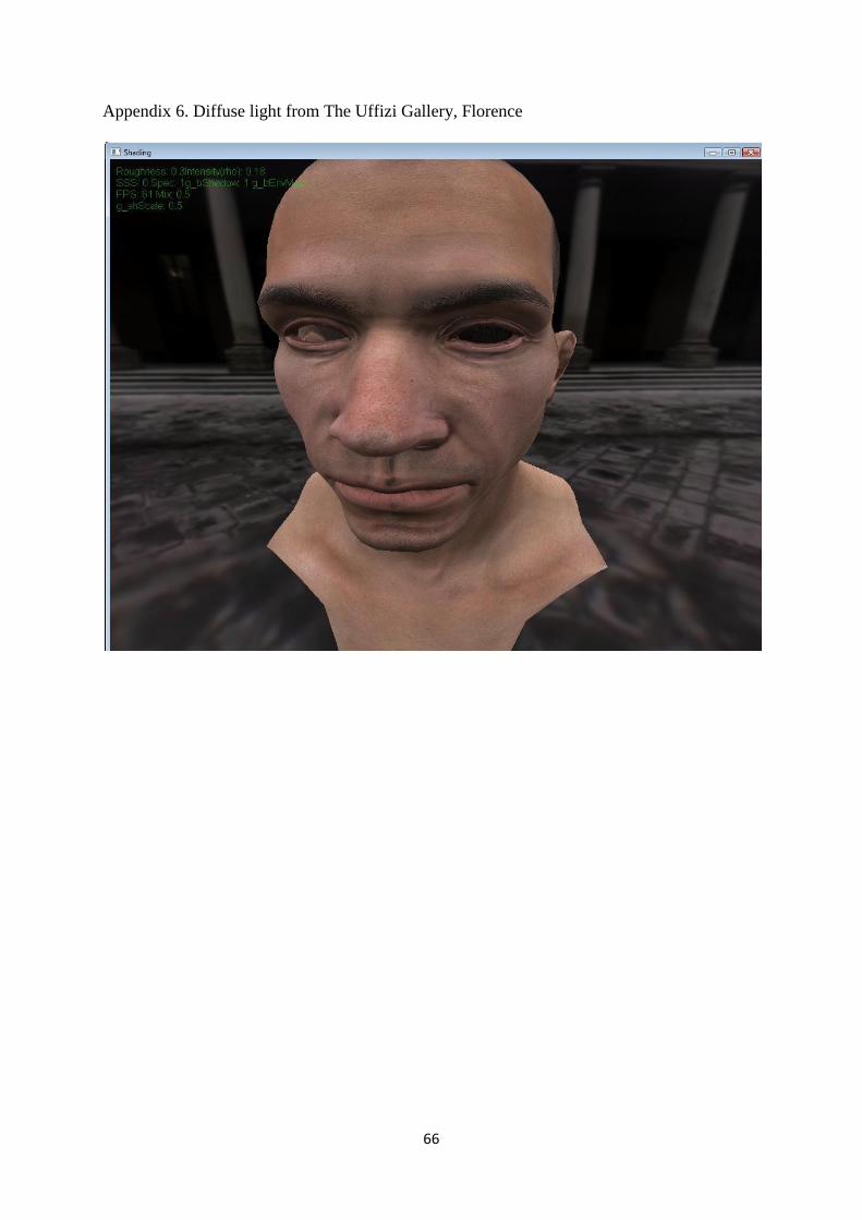
66
Appendix 6. Diffuse light from The Uffizi Gallery, Florence

67
Appendix 7. Diffuse light with applied subsurface scattering

68
Appendix 8. Diffuse light from Eucalyptus Grove, UC Berkeley
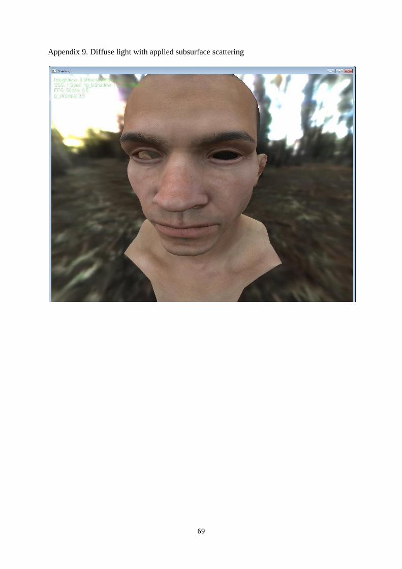
69
Appendix 9. Diffuse light with applied subsurface scattering

70
Appendix 10. Diffuse light from Galileo's Tomb, Santa Croce, Florence
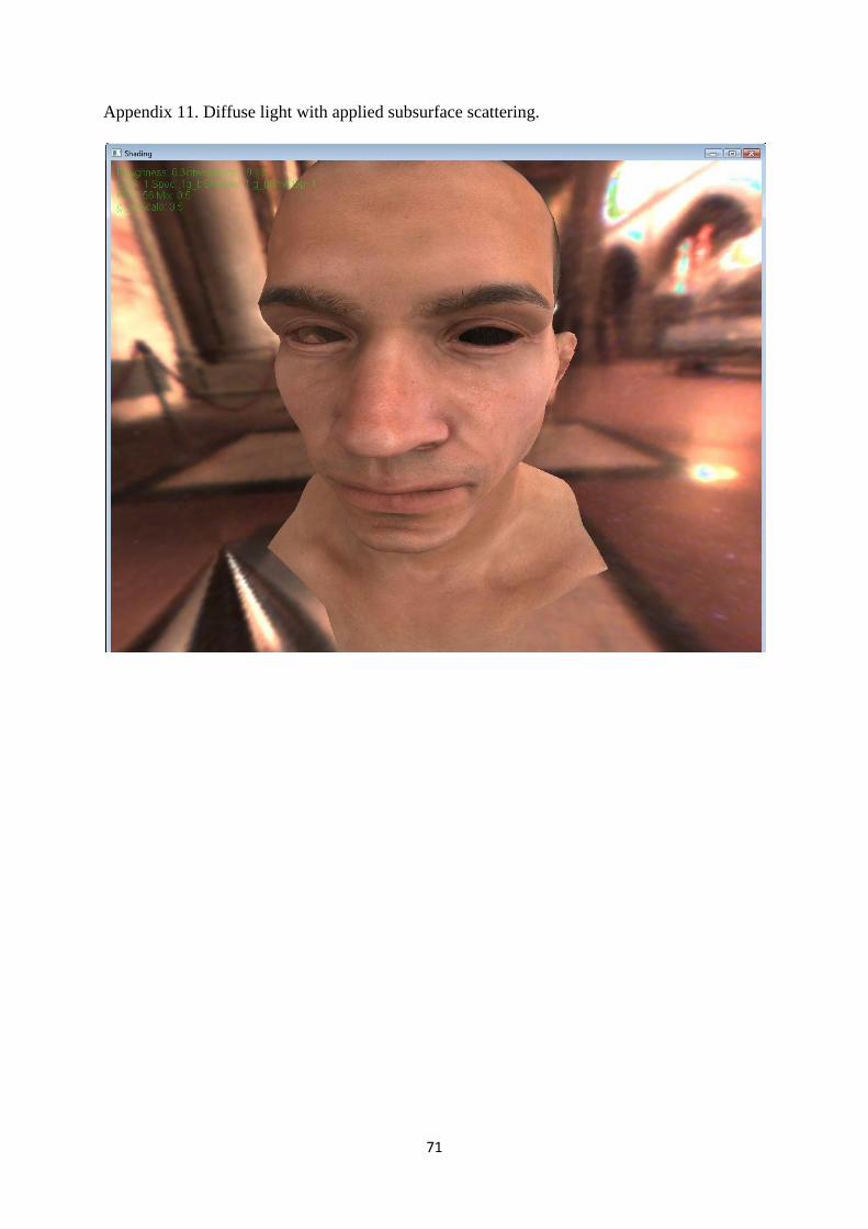
71
Appendix 11. Diffuse light with applied subsurface scattering.

72
Appendix 4. Specular reflection - Soho wavelets, BRDF - Cook-Torrance

73
Appendix 5. Specular reflection - Soho wavelets, BRDF - Kelemen/Szirmay-Kalos

74
Appendix 6. Specular reflection - Halo3, BRDF - Cook-Torrance

75
Appendix 15. Specular reflection represented by 16 Soho wavelets coefficients

76
Appendix 16. Specular reflection represented by 32 Soho wavelets coefficients
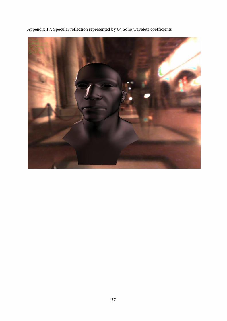
77
Appendix 17. Specular reflection represented by 64 Soho wavelets coefficients

78
Appendix 18. Specular reflection represented by 256 Soho wavelets coefficients

79
Appendix 19. Specular reflection represented by 512 Soho wavelets coefficients

TRITA-CSC-E 2009:085 ISRN-KTH/CSC/E--09/085--SE
ISSN-1653-5715
www.kth.se