Limit and Shakedown Analysis for Plastic Design

M. Staat, M. HeitzerInstitute for Safety Research and Reactor Technology,

Forschungszentrum Julich GmbH, D-52425 Julich, Germany

Abstract

Limit and shakedown theorems are exact theories of classical plasticity for the di-rect computation of safety factors or of the load carrying capacity under constantand varying loads. Simple versions of limit and shakedown analysis are the basisof all design codes for pressure vessels and pipings. Using Finite Element Methodsmore realistic modeling can be used for a more rational design. The methods canbe extended to yield optimum plastic design. In this paper we present a first im-plementation in FE of limit and shakedown analyses for perfectly plastic material.Limit and shakedown analyses are done of a pipe–junction and a interaction diagramis calculated. The results are in good correspondence with the analytic solution wegive in the appendix.

1 NOMENCLATURE

b body force���

max. plastic dissipationn outer normal vector ��������� ���������� load, limit and shakedown factorp surface traction � actual strain��� ��� � reference load ��� elastic strain� � density of plast. dissipation �����! � � plastic strain and rate"

time ��# thermal strainx coordinate vector $%�&$�'(��$*) parameters+ element compatibility matrix ,��- , residual stress and rate. �0/1�324�32 � �32�5 dimensions of the pipe–junction , dicrete eigen–stress vectorE elasticity tensor 6, time–independent residual stress798

number of Gaussian points : actual stress7<;number of load vertices = � yield stress� � �?> ��� �?> ��@BAC�DFE actual and elastic pressure : � fictitious elastic stressGIH "&J � � ��� �� load and limit pressure : � discrete fict. elast. stress vector� @ �LKMKLKB� �ON actual stresses P yield function

�Q��� > � actual and elastic temperature R , S-R structure and its boundary� ��� @ inner and outer temperature T load domain

1 Introduction

Passive components in power plants are designed on a structural mechanics basis forinternal pressure, additional mechanical loading, and thermal loading. Mechanical andthermal stress respectively decrease and increase with wall-thickness. The elastic range isbounded by allowable stress. If design is based on elastic stress assessment, the minimumtotal stress UWVXU%Y[Z0\^]-_`U?aD]bZ&c3Y may define the optimum wall-thickness of a heat exchangertube for given heat flow density.

Staat – 1

The elastic strain range is rather small. It is impossible to design a structure withconsiderable thermal loading within the elastic range. Thermo-shock or other residualstresses may push stress further into the plastic range locally. Therefore plastic analysisis used in design of passive components made of ductile material. Plastic design cannotbe based on stress assessment, because there is no stress to bound the plastic range fromfailure domains. Instead plastic design has to consider the characteristic development ofplastic strains towards structural failure [?]:

� Instantaneous collapse by unrestricted plastic flow at limit load.

� Incremental collapse by accumulation of plastic deformations over subsequent loadcycles (ratchetting).

� Low Cycle Fatigue (LCF) by alternating plasticity.

� Plastic instability of slender compression members (limit analysis does not applyfor this failure mode).

The above optimum wall-thickness may not be a rational choice for inelasticity. Plasticfailure modes cannot be assessed from the state of stress, because different stresses inter-act in a nonlinear way towards structural failure. Design codes try to maintain the stressassessment by introducing e.g. the concept of primary and secondary stress. Secondarystress is defined to have no influence on the limit load. There is little guidance for thedesigner how to recognize secondary stress. However, it is known from limit analysis thatthermal stress and all other residual stresses are secondary stresses, provided they do notsignificantly alter the geometry of the structure or the yield surface of its material [?] (forexperimental evidence see [?]).

In principle the possible structural failure may be reproduced in a detailed incremen-tal plastic analysis if it can be continued towards the limits. Generally this is prohibitivelyexpensive in the design stage and the necessary details of load history or or of the con-stitutive equations may not be available. If computation is stopped away from the limit,any prediction of failure is based on extrapolation. In particular the elastically computedstress may be of little use in limit load prediction, because limit load is independent of theelastic constants (Young’s modulus, Poisson ratio) [?].

To avoid the above short-comings ”Limit- and shakedown load form - in this or an-other way - the basis of the design concept of modern design codes such as ASME-Code,Section VIII-Division 2, British Standard 5500, ISO-DIS 2694 and the AD-Merkblatter.”([?], translated from the German). Load is the most modern word in this quotation. Com-ponent geometry, dimensions and design operation are determined by the allowable load.This design load may not be simply derived from the detailed knowledge of stress andstrain history. The interpretation of stress and stress components is not self-evident [?].The direct computation of the load carrying capacity is the objective of limit- and shake-down analyses (not applicable for the stability problem). They are used for design in theform of rules to derive allowable stress intensities [?], limit load formulae [?], and inter-action diagrams (like Bree and Brussels diagrams, [?]). This current design practice restson simplifying assumptions for geometry, loading and constitutive equation.

Staat – 2

We will show in this contribution how these assumptions may be avoided by usingthe Finite Element Method (FEM) for limit- and shakedown analysis. Some twenty yearsago the Pressure Vessel and Piping Division of ASME has invited researchers to developsoftware for design by limit analysis using the FEM [?]. But until recently this approachwas limited to relatively small Finite-Element-Models [?]. We have implemented limitand shakedown analysis into the general purpose FEM program PERMAS employing asubspace technique which can handle large models. FEM based limit and shakedownanalyses may be used to compute interaction diagrams for any complex component undertwo-parameter loading. These may be used to decide on allowable loading ranges forthe structure. More complex loading may be analysed. But they cannot be representedin a similarly visual manner. The analyses may be performed at computing times andcosts of only 2-10 standard elastic FEM analyses. Thus design variants may be comparedand an optimum choice be made [?]. The present FEM implementation of this ongoingresearch is restricted to ideal plasticity with constant material coefficient. The extensionto hardening material will be one of the next steps.

Limit and shakedown analysis may be extended towards optimum plastic design.This option was e.g. realized by the program CEPAO (Calcul Elasto-Plastique, Analyse-Optimisation) for plane frame structures [?]. The optimum cross sections of the beams inthe structure are obtained and checked for buckling of compression members. A devel-opment towards optimum plastic design could be a follower of the present project. Fromthe computational burden it is clear that the highly effective limit and shakedown analysiswill be the only possible approach for a long time [?].

Limit and shakedown theorems provide rules and guidance for design. It is e.g. eas-ily shown that adding of weightless material may not decrease the limit load [?]. In theappendix we prove, that for a structure made of linear kinematic hardening material whichfails locally under proportional loading (e. g. pressure and temperature), the shakedownrange is obtained by expansion of the elastic range by a factor of 2. This simple result isindependent of the hardening exponent and holds also for perfect plastic material. There-fore the kinematic hardening effect bears no profit for such structures (e. g. pipe–junction,plate with a hole, see [?]).

2 Theorems of limit load and elastic shakedown

Although being simplifying methods limit and shakedown analyses are exact theoriesof plasticity, which do not contain any restrictions or assumptions other than sufficientductility of the material. Simplicity is achieved with respect to the required input dataand to reduced computational effort. This is reached by restricting analysis to the directcomputation of the safety factor.

Static theorems are formulated in terms of stress and define safe structural statesgiving an optimization problem for safe loads. The maximum safe load is respectively,the limit load avoiding collapse and the (elastic) shakedown load avoiding ratchetting andLCF. Alternatively, kinematic theorems are formulated in terms of kinematic quantitiesand define unsafe structural states yielding a dual optimization problem for the minimum

Staat – 3

of limit or shakedown loads. Any admissible solution to the static or kinematic theoremis a true lower or upper bound to the safe load, respectively. Both can be made as closeas desired to the exact solution. If lower and upper bound coincide the exact solution isfound. To obtain conservative solutions the static approach is used, which is also numeri-cally more convenient.

Static limit load theorem:An elastic–plastic structure will not collapse under monotone loads if it isin static equilibrium and if the yield function is nowhere violated. The limitload is the maximum safe load.

Static shakedown theorem:An elastic–plastic structure will not fail with macroscopic plasticity undertime variant loads if it is in static equilibrium, if the yield function is nowhereand at no instance violated, and if all plastic deformations fade away, i.e. if�����a����

��� ���� V�� . The shakedown load is the maximum safe load.

If observation starts after few cycles, there may be no difference between pure elasticbehaviour and shakedown, because in elastic shakedown the material becomes eventuallyelastic. A difference can only be made if the plastic part of the load history is known.

To make them operational we will now formalize the static theorems. The givenstructure � is assumed to be composed of material points denoted by their coordinatevectors ����� . In the geometrically linear theory an additive decomposition in elastic,plastic and temperature strains of the strains is possible.

V �� _ �� _ ���� (1)

The elastic strains � V "!$#&%(' are obtained from the inverse of the fourth–orderelasticity tensor E by Hooke’s law. For an elastic, perfectly plastic material plastic strains � occur if a yield function ) reaches the yield stress U+* (and a loading condition issatisfied). The von Mises yield function is chosen. This function is prefered because itis continuous differentiable. But most theorems of plasticity theory hold also for Trescayield function. Material stability in the sense of Drucker’s postulate is assumed. Thus theyield surface bounded by , V U.-* is convex.

For a load increasing with load factor / the above necessary conditions for a safestate of � with traction boundary 01��2 (with outer normal 3 ) and yield function , underbody forces /.4 and surface loads /�5 read

, ' � 6 U -* ��7 � (2)89��: ' V /.4 ��7 � (3)

';3 V /.5 < 7 01�=2 � (4)

The limit load factor /1>@?FY�?FaIV �BADC / is a safety factor. This leads to the mathematicaloptimization problem formulated in static quantities (stress ' )

�EAFC / (5)

such that (s. t.) restrictions (2) – (4) hold � (6)

Staat – 4

The concepts for time-variant loading are more involved. Time is denoted by � . Thestresses ' can be decomposed into fictitious elastic stresses ' � and residual stresses � by

' V ' � _�� � (7)

' � V� % are stresses which would appear in an infinitely elastic material, so that the �result from plastic deformations.

The residual stresses (eigen stresses) � satisfy the homogeneous static equilibriumand boundary conditions

89��: � V�� ��7 � (8)� 3 V�� < 7 01�=2 � (9)

One criterion for an elastic, perfectly plastic material to shake down elastically is that theplastic strains � and therefore the residual stresses � become stationary for given loads� ��� V 4�� 5 � in a load domain � :

�����a����

� ��� ��� V ��������a����

� ��� ��� V���� C � � � (10)

In every considered failure mode exist points x of the structure where condition (10) isviolated. Thus there exists at least one point x for which the density of the plastic energydissipation ��� per unit volume

��� ��� ��� V a* '

����� � � ����� ��� � (11)

increases indefinitely in time. To avoid the possibility of plastic failure the maximumpossible plastic energy dissipation�

� � � V �����a���� ��� ��� ��� 6�� � � (12)

must be bounded above for all points � � � . We restrict ourselves to the shakedowncriterion (10). This means, that independent of the loading history the system has toapproach asymptotically an elastic limit state. For details of the extended theorem see[?]. The following static shakedown theorem holds [?], [?]:

Theorem (Melan):

If there exists a factor /���� and a time-independent residual stress field �� � �with �� �� %� %��� � ���� , such that for all loads

� ���� �!�,#" /�' � ��� ��� _$�� � �&%.6 U -* � � � (13)

is satisfied, then the structure will shake down elastically under the given loaddomain � .

Staat – 5

The greatest value /���� which satisfies the theorem is called shakedown-factor. The staticshakedown theorem is formulated in terms of stresses and gives a lower bound to /���� . Adual formulation in the sense of mathematical optimization is given by Koiter’s kinematictheorem [?], which is formulated in terms of kinematic quantities and yields an upperbound of /���� . The objective of limit and shakedown analyses is to find bounds to thelimit– and shakedown–factors / > ?FY ?�a and /���� . This leads to the mathematical optimizationproblem

�BADC / (14)

s. t. ,#" /�' �� ��� ��� _ �� � � % 6 U -* � � � (15)89��: �� � � V � � � � (16)�� � � 3 V � � � 01�=2 (17)

with infinitely many restrictions, which is reduced to a finite problem by FEM discretiza-tion. Shakedown analysis gives the largest range in which the loads may safely vary witharbitrary load history. If the load domain � shrinks to the point of monotone load, limitanalysis is obtained as special case.

In the case of a temperature–dependent yield function , �� � the shakedown theoremof MELAN should be modified (see [?], [?]).

3 Discretization and optimization

The structure is divided into finite elements with � Gaussian points � . The generalpurpose FEM program PERMAS [?] was chosen to implement Melan’s theorem, becauseit is sufficiently open to the user allowing to implement limit and shakedown analysis,which means a radical departure from current FEM concepts and solution steps, withoutany need of support by the PERMAS developers. PERMAS calculates the load dependentelastic stress vectors ' �? ��� by means of a displacement method [?]. The discretizedhomogeneous equilibrium conditions of the residual stresses can be noted as (see [?], [?])

���?�� #

� ? � ? V���� (18)

where the� ? are respectively the element compatibility matrices and the discrete eigen–

stress vector. This equation represents a discretized formulation of equations (16) and(17). In convex load domains � in the form of a polyhedron every load

� ��� can berepresented as a convex combination

� ���� V ���� � #

� � � ������ �����! 6 � � A 7�8 ���� � #

� � V � (19)

of the �" vertices� ���� of the polyhedron. From convex optimization theory (see [?])

follows, that inequality (15) only has to be satisfied at the vertices of � . So the condition

Staat – 6

(15) should be transformed with the stresses ' �? ���� as fictitious elastic response to vertex� ���� at the Gaussian point � into

,#" /�' �? ���� _ �� ? %.6 U -* �[V � � � � � ��� � � V � � � � � � " � (20)

The _ � unknowns of the problem are / and the residual stresses �� ? . So this is a largescale optimization problem for a realistic Finite-Element-Model. Using a basis-reductionmethod (see [?]) the number of unknowns can be reduced in a subspace so that the finalconvex optimization problem has only a few unknowns (say 4,...,7). The reduced prob-lem is convex, because the restrictions and the objective function are convex. Thus everylocal minimum is a global minimum (see [?]) and a solution of the problem is unique.Instead of infinitely many restrictions and unknowns in the continuous case, after thecomplete discretization there are only � �" restrictions and � _ � unknowns. Start-ing from unpublished work of Prager this subspace technique was developed in [?] undextended in [?] (for details see also [?]). In every reduction step the problem is solved bya self-implemented SQP-method (Sequential Quadratic Programming) with augmentedLagrangian type line search function (see [?], [?]). Armijo’s step length rule and BFGSmatrix update are used. However, numerical tests show that the algorithm may becomeeven faster without any update. Because of the small numbers of unknowns and the largenumber of restrictions, the quadratic sub–problems are solved by an active–set–strategy(see [?]). Derivatives are calculated analytically avoiding automatic differentiation meth-ods.

In every sequential step�

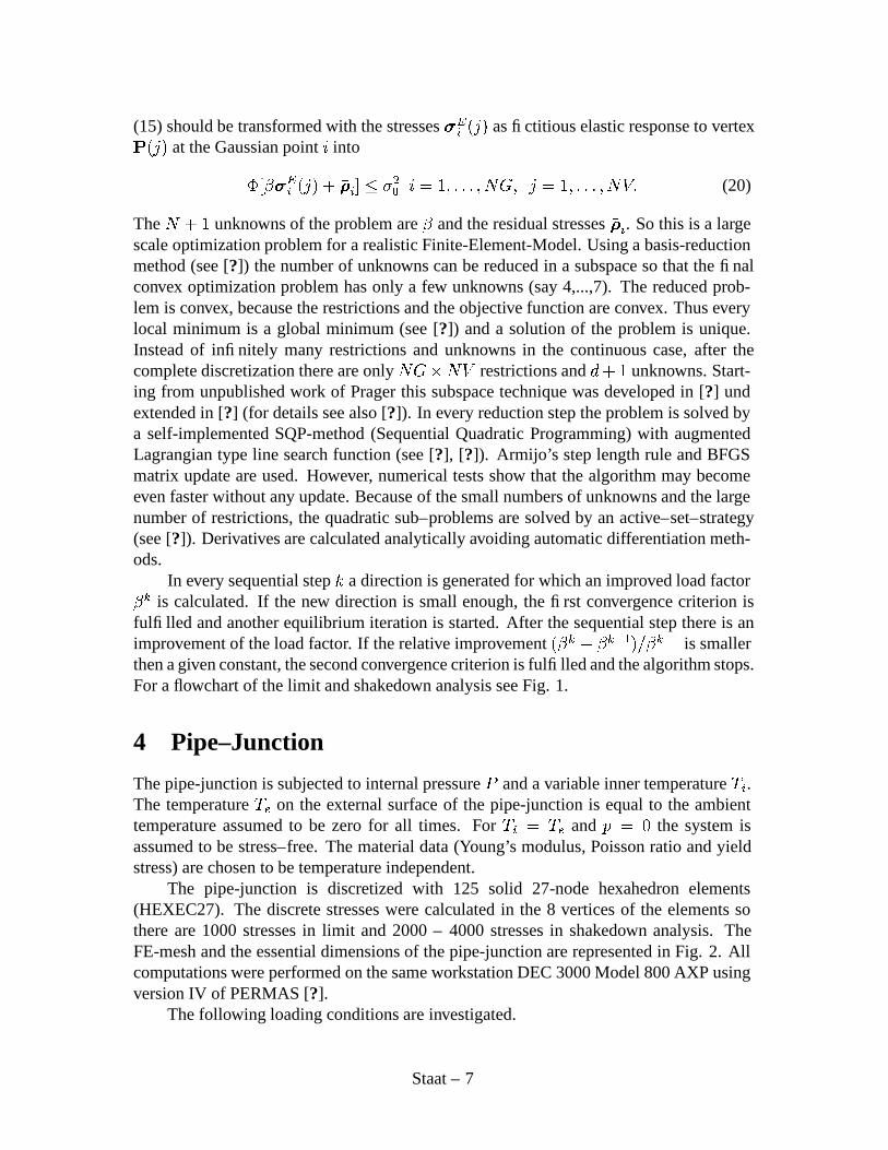
a direction is generated for which an improved load factor/�� is calculated. If the new direction is small enough, the first convergence criterion isfulfilled and another equilibrium iteration is started. After the sequential step there is animprovement of the load factor. If the relative improvement /����&/�� !$# �� /�� !$# is smallerthen a given constant, the second convergence criterion is fulfilled and the algorithm stops.For a flowchart of the limit and shakedown analysis see Fig. 1.

4 Pipe–Junction

The pipe-junction is subjected to internal pressure and a variable inner temperature � ? .The temperature � Z on the external surface of the pipe-junction is equal to the ambienttemperature assumed to be zero for all times. For � ? V � Z and � V

the system isassumed to be stress–free. The material data (Young’s modulus, Poisson ratio and yieldstress) are chosen to be temperature independent.

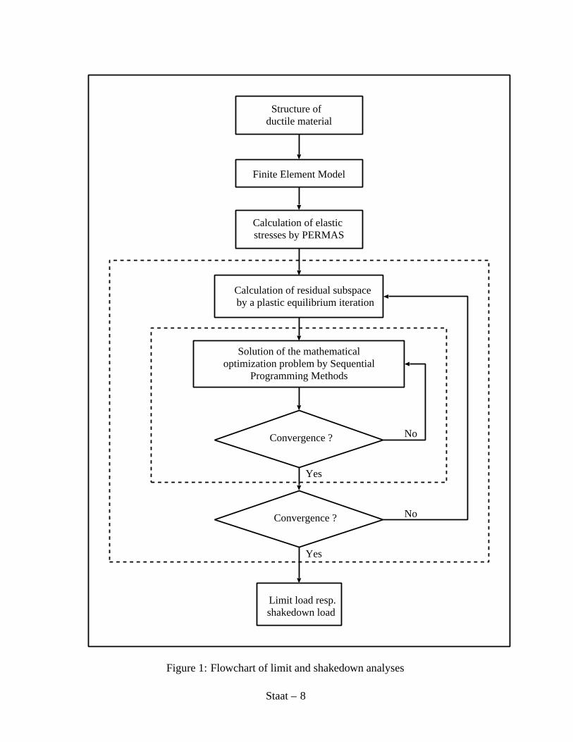
The pipe-junction is discretized with 125 solid 27-node hexahedron elements(HEXEC27). The discrete stresses were calculated in the 8 vertices of the elements sothere are 1000 stresses in limit and 2000 – 4000 stresses in shakedown analysis. TheFE-mesh and the essential dimensions of the pipe-junction are represented in Fig. 2. Allcomputations were performed on the same workstation DEC 3000 Model 800 AXP usingversion IV of PERMAS [?].

The following loading conditions are investigated.

Staat – 7

Finite Element Model

Calculation of elastic stresses by PERMAS

Yes

Limit load resp. shakedown load

Structure of ductile material

Calculation of residual subspace by a plastic equilibrium iteration

No

Solution of the mathematical optimization problem by Sequential

Programming Methods

Convergence ?

Yes

No

Convergence ?

Figure 1: Flowchart of limit and shakedown analyses

Staat – 8

1. Pressure and temperature � ? vary simultaneously with �� V ������� � � (one–parameter loading):

6 6 / � * � 6 � ? 6 / � � * � 6 � 6 � �

�* and � * are a reference pressure and temperature, respectively.

2. Pressure and temperature � ? vary independently (two–parameter loading)

6 6 / � # * � 6 �#6 �

6 � ? 6 / � -� * � 6 � -

6 � �Additionally the two cases � * 6

and � * � were studied. This corresponds to the cases� ? 6 ��� and � ? � ��� , respectively. We obtain the collapse pressure by setting � * V

.In limit analysis the internal pressure at first yield in the symmetry plane at the inner

nozzle corner is calculated to Z > �� a ?F\ � � ���� U$* . Numerical limit analysis with thebasis-reduction technique leads to a collapse pressure of � � � � Z > �� a ? \ V � �����1U$* . Forcomparison the limit pressure resulting from the German design rules AD-Merkblatt B9is calculated to >@?�Y ?Fa�V�� � � � Z > �� a ? \ V � ����� U$* (see [?]).

R A P SISR-FZ JUELICH

0.0 -36.0 -37.0

XY

Z

. ......................................................................................................................................................................................................................................................................................................................................................................................................................................................................................................................................................................................................................................................................................................................................

.....................................................................................................................................................................................................................................................................................................................................................................................................................................................................................................................................................................................................................................................................................................................................

.........................................................................................................................................................................................................................................................................................................................................................................................................................................................

�� �

�

� ��� �"!$#&%�%' ()�*++

Ø

, ()-

� �Ø . �0/�1

.....................................................................................................................................................................................

................................................

................................................

....................................

............................................................

....................................

........................................................................

......................................................................................... .................

2 2 2 2 2 2 2 2 2 2 2 2 2 2 2 2 2 2 2 2 2 2 2 2 2 2 2 2 2 2 2 2 2 2 2 2 2 2 2 2 2 2 2 2 2 2 2 2 2 2 2 2 2 2 2 2 2 2 2 2 2 2 2 2 2 2 2 2 2 2 2 2 2 2 2 2 2 2 2 2 2 2 2 2 2 2 2 2 2 2 2 2 2 2 2 2 2 22 2 2 2 2 2 2 2 2 2 2 2 2 2 2 2 2 2 2 2 2 2 2 2 2 2 2 2 2 2 2 2 2 2 2 2 2 2 2 2 2 2 2 2 2 2 2 2 2 2 2 2 2 2 2 2 2 2 2 2 2 2 2 2 2 2 2 2 2 2 2 2 2 2 2 2 2 2 2 2 2 2 2 2 2 2 2 2 2 2 2 2 2 2 2 2 2 2

2 2 2 2 2 2 2 2 2 2 2 2 2 2 2 2 2 2 2 2 2 2 2 2 2 2 2 2 2 2 2 2 2 22 2 2 2 2 2 2 2 2 2 2 2 2 2 2 2 2 2 2 2 2 2 2 2 2 2 2 2 2 2 2 2 2 22 2 22 22 22 2 22 22 22 22 22 22 22 22 22 22 22 22 22 22 22 22 22 22 2

2 2 2 2 2 2 2 2 2 2 2 2 2 2 2 2 2 2 2 2 2 2 2 2 2 2 2 2 2 2 2 2 2 2 2 2 2 22 2 2 2 2 2 2 2 2 2 2 2 2 2 2 2 2 2 2 2 2 2 2 2 2 2 2 2 2 2 2 2 2 2 2 2 2 22 22 22 22 22 22 22 22 22 22 22 22 22 22 22 22 22 22 22 22 2

Figure 2: FE-mesh and dimension of a Pipe-Junction

From thick shell theory (see [?]) the pure elastic pressure 3[Z > �� a ?F\ of the correspondingundisturbed pipe is

3[Z > �� a ?F\ V 54 _6� �F� - � 4 -7 � 84 _6� �D� - U$*9� � ��: U$* � (21)

The limit load factor 3/$>@?�Y ?Fa corresponding to 3[Z > �� a ?F\ (see [?]) is

3/$> ?FY�?FaQV 2 ln ; 4 _6� �4 <� �=; 44 _6� � < - � �

� ��� � � (22)

Staat – 9

Thus the collapse pressure 3�>@?FY�?Fa of the undisturbed pipe is

3 > ?FY ?�aQV 3/$> ?FY�?Fa 3[Z > �� a ?F\ � � � � � U$* (23)

instead of � �����1U1* for the pipe–junction. The junction presents a 28% weakening of the

structure. Comparison with the elastic limit � �� ��:�U * shows, that there is a benefit of

more than 181% in the ultimate load carrying capacity.CLOUD and RODABAUGH in [?] (see also [?]) gave an upper bound on the limit

pressure of a pipe–junction with

Inner pipe radius 4 V � � � � ��� mmInner junction radius � V�� � � : mmPipe thickness � � V�� � � � mmJunction thickness � � V � � � � mm.

With � V�4 and � V � 4� � (24)

and the approximation formula of CLOUD and RODABAUGH the collapse pressure �>@?FY�?Fais

�>@?�Y ?Fa V� � -�� � - _

� -�� � -� �!_ �� 7 ��� _ � � � �� � � _

� ��� ��:� � � _

� �� ��� - � 7 ���� �� � _ � �� � - � _ ��:� � � � 7 � _ �� 7 � U$*

� � � ��U$* � (25)

The elastic pressure 3[Z > �� a ? \ of the undisturbed pipe calculated by thick shell theory yields

3 Z > �� a ? \ � � :�� U$* � (26)

The limit load factor is 3/$>@?FY�?Fa V � � � � and the corresponding collapse pressure is

3 > ?FY�?Fa � � : : U$* � (27)

Thus the junction presents a 50 % weakening of the pipe. The result of the simple for-mula (25) ( >@?�Y ?Fa V � � ��U$* ) shows good agreement with the experimental results ofSCHROEDER in [?] ( >@?�Y ?Fa�V � � � U$* ).

For the pipe–junction benchmark example ( > ?FY�?Fa V � ��� � U$* ) the result of equation(25) is not meaningful. Equation (25) yields >@?�Y ?Fa V � � � � U$* , but the collapse pressureof the undisturbed pipe is only 3 > ?FY ?�a V � ��: U$* . So the upper bound on the limit pres-sure given by the equation of CLOUD and RODABAUGH in [?] is not applicable to thebenchmark example. Perhaps the greater ratio � � ��4 V � ����: in the benchmark exampleinstead of � � ��4 V � � � in SCHROEDER’s experiment explains the differences.

The stresses corresponding to the thermal loading are residual stresses. So the tem-perature loading has no influence on the limit pressure for one– and for two–parameter

Staat – 10

el.

-2

-1

1 2 2.85

T / T el.

Elastic Load Range

P / P

1

2

Limit Load Range

Shakedown Load Range (prop.)Shakedown Load Range

Figure 3: Interaction diagram of the pipe-junction

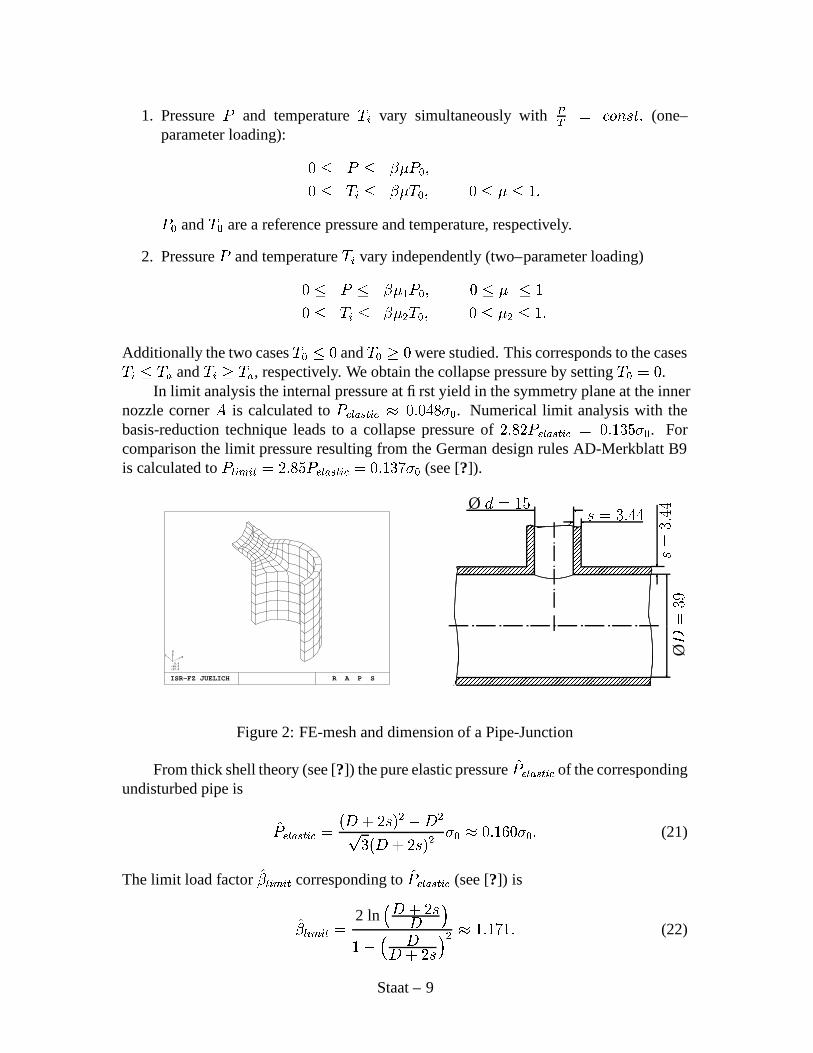
loading. Therefore in the interaction–diagram (see Fig. 3) of the pipe-junction the limitload range is a straight line parallel to the ordinate (the long–dashed curve). The axes ofordinates and abscissa are normed to elastic temperature–stress and to elastic pressure, re-spectively. The short–dashed curve in Fig. 3 marks the elastic load range in proportionalloading. The kink in the line means, that for small ratio of temperature load to pres-sure load the presence of temperature load increase the possible pressure load to initialyielding.

The short–long–dashed curve marks the shakedown load range corresponding to thefirst loading condition. The shakedown factor is nearly 2 for all proportionality factors.The pipe–junction fails in every case locally at the inner nozzle point so that the factor 2is analytical guaranteed (see the appendix for an analytic solution).

The solid curve marks the shakedown load range for two–parameter loading. The

Staat – 11

shakedown factor varies between 1.46 and 2 related to the elastic load range.The dimension of the residual subspace is growing during the iteration from 3 to 5.

So the optimization problem has 4-6 unknowns and 2000 restrictions for one–parameterand 4000 restrictions for two–parameter loading.

The additional CPU-time for shakedown analysis is less than twice the time for thelinear elastic analysis which shows, that in this case shakedown analysis is faster thanlimit analysis and it is much faster than computing through 10-100 inelastic load cyclesuntil shakedown may be observed.

From an incremental calculation of the pipe–junction subjected to internal pressurewe get a pressure–strain–curve (see Fig. 4). The picture shows the relation between themaximal reference strain at the inner nozzle corner A and the applied inner pressure. Theaxes of ordinates and of abscissa are normed to elastic pressure and strain at point A,respectively.

A

P / Pel

0.5

1

1.5

2

2.5

Ael

e

ε / εA1 2 3 4 5 76

c

d

g

bf

a

Figure 4: Pressure–strain–curve for point A of the pipe-junction

After initial elastic loading there is an increase of the loading until twice the elastic pres-sure is reached. Then the structure is un– and reloaded up to the previous load and above.The un– and reloading part of the curve is a line parallel to the initial elastic curve. Thereis no difference in the whole loading curve if there is a unloading during the loading.This means that the ultimate pressure is independent of the load–history. The remainingplastic reference strain at point A is the distance between the origin and the intersectionpoint of the curve and the abscissa. This strain corresponds with the remaining residualstresses at point A. These normally unknown residual stresses could result from an initialloading or from the production process. However, they do not effect the ultimate pressure.

Staat – 12

This effect corresponds to the experiments with bar–structures of MAIER–LEIBNITZ [?].Therefore limit analysis needs no information about the load history. But it cannot predictunique strains at collapse and it must assume sufficient ductility.

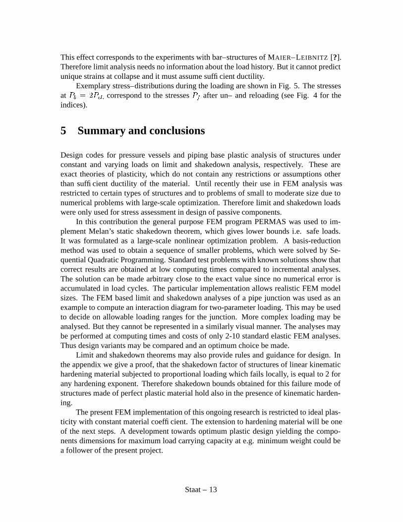
Exemplary stress–distributions during the loading are shown in Fig. 5. The stressesat �� V � [Z >�� correspond to the stresses �� after un– and reloading (see Fig. 4 for theindices).

5 Summary and conclusions

Design codes for pressure vessels and piping base plastic analysis of structures underconstant and varying loads on limit and shakedown analysis, respectively. These areexact theories of plasticity, which do not contain any restrictions or assumptions otherthan sufficient ductility of the material. Until recently their use in FEM analysis wasrestricted to certain types of structures and to problems of small to moderate size due tonumerical problems with large-scale optimization. Therefore limit and shakedown loadswere only used for stress assessment in design of passive components.

In this contribution the general purpose FEM program PERMAS was used to im-plement Melan’s static shakedown theorem, which gives lower bounds i.e. safe loads.It was formulated as a large-scale nonlinear optimization problem. A basis-reductionmethod was used to obtain a sequence of smaller problems, which were solved by Se-quential Quadratic Programming. Standard test problems with known solutions show thatcorrect results are obtained at low computing times compared to incremental analyses.The solution can be made arbitrary close to the exact value since no numerical error isaccumulated in load cycles. The particular implementation allows realistic FEM modelsizes. The FEM based limit and shakedown analyses of a pipe junction was used as anexample to compute an interaction diagram for two-parameter loading. This may be usedto decide on allowable loading ranges for the junction. More complex loading may beanalysed. But they cannot be represented in a similarly visual manner. The analyses maybe performed at computing times and costs of only 2-10 standard elastic FEM analyses.Thus design variants may be compared and an optimum choice be made.

Limit and shakedown theorems may also provide rules and guidance for design. Inthe appendix we give a proof, that the shakedown factor of structures of linear kinematichardening material subjected to proportional loading which fails locally, is equal to 2 forany hardening exponent. Therefore shakedown bounds obtained for this failure mode ofstructures made of perfect plastic material hold also in the presence of kinematic harden-ing.

The present FEM implementation of this ongoing research is restricted to ideal plas-ticity with constant material coefficient. The extension to hardening material will be oneof the next steps. A development towards optimum plastic design yielding the compo-nents dimensions for maximum load carrying capacity at e.g. minimum weight could bea follower of the present project.

Staat – 13

R A P SISR-Fz Juelich

PIPE JUNCTION

0.0 -30.0 -30.0

XY

Z

1.178E+03 4.581E+03 7.984E+03 1.139E+04 1.479E+04 1.819E+04 2.160E+04 2.500E+04

N/MM**2

STRESSES, SIGMA VM R A P SISR-Fz Juelich

PIPE JUNCTION

0.0 -30.0 -30.0

XY

Z

2.766E+03 5.943E+03 9.119E+03 1.230E+04 1.547E+04 1.865E+04 2.182E+04 2.500E+04

N/MM**2

STRESSES, SIGMA VM

� V Z > � � V � [Z >��

R A P SISR-Fz Juelich

PIPE JUNCTION

0.0 -30.0 -30.0

XY

Z

2.766E+03 5.943E+03 9.119E+03 1.230E+04 1.547E+04 1.865E+04 2.182E+04 2.500E+04

N/MM**2

STRESSES, SIGMA VM R A P SISR-Fz Juelich

PIPE JUNCTION

0.0 -30.0 -30.0

XY

Z

2.766E+03 5.943E+03 9.119E+03 1.230E+04 1.547E+04 1.865E+04 2.182E+04 2.500E+04

N/MM**2

STRESSES, SIGMA VM

\ V Z > � � V

R A P SISR-Fz Juelich

PIPE JUNCTION

0.0 -30.0 -30.0

XY

Z

2.766E+03 5.943E+03 9.119E+03 1.230E+04 1.547E+04 1.865E+04 2.182E+04 2.500E+04

N/MM**2

STRESSES, SIGMA VM R A P SISR-Fz Juelich

PIPE JUNCTION

0.0 -30.0 -30.0

XY

Z

2.766E+03 5.943E+03 9.119E+03 1.230E+04 1.547E+04 1.865E+04 2.182E+04 2.500E+04

N/MM**2

STRESSES, SIGMA VM

[Z V [Z >�� � V�� [Z >��

R A P SISR-Fz Juelich

PIPE JUNCTION

0.0 -30.0 -30.0

XY

Z

2.766E+03 5.943E+03 9.119E+03 1.230E+04 1.547E+04 1.865E+04 2.182E+04 2.500E+04

N/MM**2

STRESSES, SIGMA VM

��IV � � � Z > �Figure 5: Pressure–strain–curve for point A of the pipe-junction

Staat – 14

6 Appendix

For structures made of linear kinematic hardening material the shakedown behaviour isdominated by some points of the structure, where the maximum expansion of the elasticdomain is the minimum over all points � � � :

/���� V � ��7��� � �BADC� / � � (28)

If only one point dominates the behaviour it is possible to solve the optimization prob-lem analytically. In this case the shakedown load for perfectly plastic and linear kine-matic hardening material correspond (see [?]). Zhang solved the problem in [?] for two–dimensional structures in two–parameter loading domain (e.g. plate with a circular holesubjected to biaxial tension) STEIN and HUANG solved the problem in principal stressspace (see [?]) by the mathematical program MACSYMA. We solved the shakedownoptimization problem analytically for linear kinematic hardening material in the case oflocal failure in one–parameter loading without the need of principal stresses. The back-stresses � have no restrictions in the case of linear kinematic hardening material, so that� V � ��� has no restrictions. Assuming that the maximum effective stress would ap-pear at one point of the system, then we need to solve the optimization problem with thebackstresses � and

� ��7� / (29)

�� � � � � , / ' �� _ � � 6 U -* � V � � � � � � �" (30)

only in this point (see [?]). The corresponding LAGRANGE function is defined as

� /�� � � V � / � ���� � #� � " U -* �;, /�' �� _ � �&% � (31)

With the abbreviation ' � %�V�' �� it holds

, /�' � _ � � V / - ' �� ' � _ � /�' �� � _ � � � (32)

V /�� � � � � ' �� ' � ' �� ' � �� �� ���� ���

� /� � � (33)

In three dimensional problems the matrix ����������� is defined by the von Mises function

� �!""""""#

$ % ') % ') &'&(&% ') $ % ') &'&(&% ') % ') $ &'&(&& & & )'&(&& & & &')(&& & & &'&()

*,++++++- K (34)

Staat – 15

With � %FV /�� � � � and � ����� � the short form of (31) is

� � � V � � � � � � � � � � � ���� � #� � " U -* ��� � � � � % A 7�8 (35)

��� � � V � � � � � � � � � � _6� ���� � #

� � � � � (36)

with the differential operator��� �� � V ; ���� ��� � � �� ����� � � � � � ����� ����� < . From the KUHN–TUCKER–

conditions��� ��� � V � of a local minimum ��� V /�� � � � � � it follows (see [?]) with the

optimal LAGRANGE multipliers���

� � � � � � � � V �!# ���� � #��� � �*- � � V � ���� � #

���� ' �� ' � ' �� ' � � � � (37)

V �!""""#

���� � #��� ' �� ' �

� ���� � #��� ' � � �

� ���� � #��� ' � � � ��

�� � #��� �

*,++++- � � � (38)

In the local minimum � � the complementary condition of every restriction reads:��� U -* ��� � � � � � � � V � V � � � � � �� " � (39)

After summation of all complementary conditions, we deduce with (37)

U -* ���� � #��� V

���� � #��� � � � � � � � V�� � �

���� � #��� � � � � (40)

V �� � � � � � � � � � � V �� / � � (41)

There is a unique representation of /�� by the LAGRANGE multipliers��� :

/ � V � U -* ���� � #��� � (42)

With (42) it follows from (38)

� V!# ���

� � #��� ' � � ���� � #

��� *- � � V�/ �

���� � #��� ' � _

!# ���� � #���*- � � (43)

V / � ���� � #��� ' � _ /��� U -* � � � (44)

and with / � �

� � V � �1U -* ���� � #��� ' � � (45)

Staat – 16

Now with (37) it follows

�� V!# ���� � #��� ' �� ' � � ���� � #

��� ' ��

*- � � (46)

V / � ���� � #��� ' �� ' � _

���� � #��� ' �� � � (47)

and with (45)

� /�� ���� � #��� ' �� ' � � �� U -* V

!# ���� � #��� ' �*- � !# ���

� � #��� ' �

*-

V!# ���� � #��� ' �*- �

!# ���� � #��� ' �*- (48)

In the case of one–parameter loading the load domain in shakedown analysis has twovertices. The corresponding fictitious elastic stresses ' # and ' - with , ' #

� V and

, ' -� VXU -* to the two load vertices read

' # V � � � � � � and ' - V

�# � � - � � � ��� � ��� � � � � (49)

From (42) follows/ � V�� U -* � � # _ � �- � (50)

With (42) and (48) follows

� � # _ � �- � � �- � �� U -* V � �- U -* or�� #��- V

�� U �* � (51)

This means, that both restrictions must be active in the local maximum. From the KUHN–TUCKER–conditions and equations (42) and (51) follows

�� # V �

�- V��1U -* (52)

/ � V � � (53)

In one–parameter loading the shakedown load is twice the elastic load. This result holdsindependently of the hardening exponent and also for perfect plastic material [?]).

Staat – 17