Embed Size (px)
Citation preview
EXPERIMENTAL ANALYSIS OF LIMITATIONS IN THE
STRUT-AND-TIE METHOD
Niels Bailleul & Mikael Wahlgren
Division of Structural Engineering
Faculty of Engineering, LTH
Lund University, 2016
Rapport TVBK – 5249
EXPERIMENTAL ANALYSIS OF LIMITATIONS
IN THE STRUT-AND-TIE METHOD
Niels Bailleul
Mikael Wahlgren
2016

ii
Report TVBK-5249
ISSN 0349-4969
ISRN: LUTVDG/TVBK-16/5249 (118p)
Master’s thesis
Supervisors: Oskar Larsson and Kent Kempengren
Examiner: Annika Mårtensson
May 2016
iii
DIVISION OF STRUCTURAL ENGINEERING
FACULTY OF ENGINEERING
MASTER’S THESIS
EXPERIMENTAL ANALYSIS OF LIMITATIONS
IN THE STRUT-AND-TIE METHOD
EXPERIMENTELL ANALYS AV BEGRÄNSNINGARNA I
FACKVERKSMETODEN FÖR HÖGA
BETONGELEMENT
NIELS BAILLEUL and MIKAEL WAHLGREN
Supervisors: OSKAR LARSSON, Div. of Structural Engineering, LTH and
KENT KEMPENGREN, Div. of Structural Engineering, LTH
Examiner: Professor ANNIKA MÅRTENSSON, Div. of Structural Engineering, LTH

iv
Keywords: Strut-and-Tie method, Reinforced concrete, Concrete Damaged Plasticity,
Fracture energy
Nyckelord: Fackverksmetoden, Armerad betong, Sprickenergi
v
ABSTRACT One of the overall main purposes for a structural engineer is to design structures and structural
elements so that they meet society’s safety requirements, yet use as little material as possible.
In order to do so, the designer has to understand and simplify a complex reality. The strut-and-
tie method is such a simplification model which allows engineers to design reinforced concrete
structures where basic beam theory is not applicable, e. g. high beams or discontinuity regions
near supports and loads.
When designing according to the strut-and-tie method, several assumptions have to be made
regarding the structural behavior. Questions exists whether current recommendations regarding
these assumptions are conservative – the assumed internal truss system for ultimate limit state
calculations is usually based on the linear-elastic stress field. This despite stress redistribution
due to cracking and plastic deformations is possible. Accounting for the stress redistribution
would yield a higher load-bearing capacity in the ultimate limit state. The conservative
approach derives from uncertainties regarding the materials plastic deformation capacities and
serviceability limit state considerations.
The aim of this report is to investigate the effects on the stress distribution of a simply supported
high concrete beam when loaded to failure, investigating the redistribution capacity of the
member. In the design of the specimen, extreme cases were chosen, e.g. a structure with a very
small amount of reinforcement. Thus, the scope of the project also includes limitations in the
strut-and-tie method.
Studies were performed on four specimen with different amount of reinforcement; three
members with increasing amount of reinforcement and a fourth reinforced with a minimum
reinforcement mesh in accordance with Eurocode. The beams were simply supported and
subjected to two-point loading. Laboratory results were compared with computer simulations
and hand calculations.
Analyzing the results from the simulations indicated a rise of the internal lever arm, in three
out of four cases. The laboratory test results clearly showed two types of behavior; a brittle
failure for the ‘insufficiently reinforced’ and a ductile response from the one with minimum
reinforcement installed. Comparing the results from the lab and the model gave diverse results
in terms of stiffness.

vi
vii
SAMMANFATTNING
Ett av de övergripande syftena för en konstruktör är att utforma konstruktioner och
konstruktionselement så att de uppfyller samhällets säkerhetskrav, samtidigt som
materialanvändandet är sparsamt. För att klara av detta måste konstruktören förstå och förenkla
en komplex verklighet. Fackverksmetoden är en modell som gör det möjligt för konstruktörer
att utforma betongkonstruktioner där grundläggande balkteori inte är tillämplig, t.ex. höga
balkelement eller diskontinuitetsregioner nära stöd och laster.
Vid dimensionering enligt fackverksmetoden måste flera antaganden göras om konstruktionens
beteende. Frågor huruvida nuvarande rekommendationer gällande dessa antaganden är
konservativa finns – den interna hävarmen för beräkningar i brottgränstillstånd är baserad på
det linjär-elastiska spänningsfältet. Detta trots att ett tillgodoräknande av
spänningsomfördelning på grund av sprickor och plastiska deformationer är möjligt för
dimensionering i brottgränstillstånd. Ett sådant tillgodoräknande skulle ge högre bärförmåga.
Det konservativa förhållningssättet härstammar från osäkerheter gällande materialens plastiska
deformationskapacitet och dess respons i bruksgränstillstånd.
Syftet med denna rapport är att undersöka effekterna på spänningsfördelningen av en fritt
upplagd hög betongbalk när den belastas till brott och därigenom undersöka konstruktionens
kapacitet att omlagra spänningar. Vid utformningen av försöken valdes extrema fall,
exempelvis konstruktioner med mycket låg armeringsmängd. Således ingår också analyser av
begränsningar i metoden.
Studier utfördes på fyra prov med varierande armeringsmängd; tre provkroppar med ökande
mängd armering och en fjärde förstärkt med minimiarmeringsnät i enlighet med Eurocode.
Balkarna utsattes för tvåpunktsbelastning och var fritt upplagda. Laboratorieresultat jämfördes
med datorsimuleringar och handberäkningar.
När resultaten från simuleringen analyserades kunde utvecklingen av den inre hävarmen enkelt
konstateras. Resultaten från laborationen gav indikationer på två typer av beteende; ett sprött
brott i balken med minst armering, samt ett duktilt beteende hos balken försedd med
minimiarmering. När resultaten från de två metoderna jämfördes uppvisades dock stora
skillnader vad gäller styvhet.

viii

ix
ACKNOWLEDGEMENTS
This master’s thesis was made at the Division of Structural Engineering at the Faculty of
Engineering LTH at Lund University during the spring of 2016, starting in January and
finalized in May.
We would like to thank first and foremost our supervisors Dr. Oskar Larsson, who initiated the
idea for this thesis and for all valuable comments and hints and Ph.D. student Kent Kempengren
who we have shared a lot of headaches with in the computer modelling process and who have
always helped us when in need. We would also like to thank Prof. Emeritus Sven
Thelandersson who have offered his expertise and knowledge throughout the process.
A special thanks to research engineer Per-Olof Rosenkvist for all help and good times in the
lab; and research engineer Bengt Nilsson for the help in the advanced ‘fracture energy’ testing.
Most importantly we would like to thank each other. For enduring this process, always striving
forward and for motivating and helping one another.
This concludes a five year journey at Lund University. A time period that have shaped us to
the individuals we are today. One last thanks therefore goes to everyone that have enriched this
time, especially during the last year – the late nights in school, the ping pong tournaments and
all the interesting discussions. Thank you.
LUND, MAY 2016
x
Engineering is the art of modelling materials we do not wholly understand, into shapes we
cannot precisely analyze so as to withstand forces we cannot properly assess, in such a way
that the public has no reason to suspect the extent of our ignorance.
– Dr AR Dykes
CONTENTS
1 INTRODUCTION ............................................................................................................. 1
1.1 Background ................................................................................................................. 1
1.2 Objective ..................................................................................................................... 1
1.3 Scope & Limitations.................................................................................................... 2
1.4 Method ........................................................................................................................ 2
1.4.1 Literature study .................................................................................................... 3
1.4.2 Hand calculations ................................................................................................. 3
1.4.3 Laboratory testing ................................................................................................ 3
1.4.4 Computer modelling ............................................................................................ 3
1.5 Tested model ............................................................................................................... 4
2 BACKGROUND THEORY .............................................................................................. 7
2.1 Materials ...................................................................................................................... 7
2.1.1 Concrete ............................................................................................................... 7
2.1.2 Reinforcing Steel ............................................................................................... 12
2.1.3 Reinforced concrete ........................................................................................... 13
2.2 Stress distribution ...................................................................................................... 14
2.2.1 Linear stress distribution .................................................................................... 14
2.2.2 Non-linear stress distribution ............................................................................. 15
2.3 Design based on plasticity ......................................................................................... 17
2.4 The strut-and-tie method ........................................................................................... 18
2.4.1 Examples of applications of the strut-and-tie method ....................................... 22
2.4.2 Stress redistribution in discontinuity regions ..................................................... 23
2.5 Risk assessment and safety factors............................................................................ 25
2.6 Finite element model ................................................................................................. 26
2.6.1 Constitutive modeling using Concrete Damaged Plasticity model ................... 27
3 CALCULATION PROCEDURE .................................................................................... 35
3.1 Struts.......................................................................................................................... 36
3.1.1 Forces ................................................................................................................. 37
3.1.2 Capacities ........................................................................................................... 37
3.2 Nodes ......................................................................................................................... 38
3.2.1 Capacity of ‘Compression – Compression Node’ ............................................. 38
3.2.2 Capacity of ‘Compression – Tension Node’ ...................................................... 40
3.3 Tie.............................................................................................................................. 42
3.4 Load bearing capacity of specimen ........................................................................... 43
3.5 Anchorage length ...................................................................................................... 43
4 LABORATORY PROCESS ............................................................................................ 45
4.1 Material properties .................................................................................................... 45
4.1.1 Concrete ............................................................................................................. 45
4.1.2 Steel.................................................................................................................... 48
4.2 Manufacturing specimens ......................................................................................... 49
4.2.1 Molding cast....................................................................................................... 50
4.2.2 Reinforcement .................................................................................................... 50
4.2.3 Material test specimen ....................................................................................... 52
4.2.4 Concrete casting ................................................................................................. 52
4.3 Laboratory procedure ................................................................................................ 53
4.4 Measurements............................................................................................................ 54
5 COMPUTER MODELLING ........................................................................................... 55
5.1 Model ........................................................................................................................ 55
5.1.1 Parts.................................................................................................................... 55
5.1.2 Material properties ............................................................................................. 55
5.1.3 Loading and boundary conditions ...................................................................... 59
5.1.4 Interaction between concrete and reinforcement bars ....................................... 59
5.1.5 Time step ............................................................................................................ 59
5.1.6 Mesh ................................................................................................................... 60
6 RESULTS AND ANALYSIS .......................................................................................... 61
6.1 Material properties .................................................................................................... 61
6.1.1 Concrete – compressive strength ....................................................................... 61
6.1.2 Concrete – tensile strength ................................................................................. 62
6.1.3 Concrete – fracture energy ................................................................................. 62
6.1.4 Reinforcement – tensile strength ....................................................................... 62
6.2 Load capacity ............................................................................................................ 63
6.2.1 Primary calculations........................................................................................... 64
6.2.2 Revised calculations........................................................................................... 64
6.2.3 Laboratory test results ........................................................................................ 65
6.2.4 Computer model results ..................................................................................... 66
6.3 Comparison between model and laboration .............................................................. 67
6.3.1 T1 – Response curve .......................................................................................... 67
6.3.2 T1 – Force-strain in reinforcement .................................................................... 68
6.3.3 T2 – Response curve .......................................................................................... 69
6.3.4 T2 – Force-strain in reinforcement .................................................................... 70
6.3.5 T3 – Response curve .......................................................................................... 71
6.3.6 T3 – Force-strain in reinforcement .................................................................... 72
6.3.7 T4 – Response curve .......................................................................................... 74
6.3.8 T4 – Force-strain in reinforcement .................................................................... 76
6.4 Comparisons between specimens .............................................................................. 77
6.4.1 Deflection - Laboration ...................................................................................... 77
6.4.2 Deflection – Computer model ............................................................................ 78
6.4.3 Concrete stress field ........................................................................................... 79
6.5 Discussion ................................................................................................................. 85
7 CONCLUSIONS.............................................................................................................. 87
7.1 Conclusions from work ............................................................................................. 87
7.2 Further research ......................................................................................................... 88
REFERENCES ........................................................................................................................ 91
APPENDIX A - DRAWINGS ................................................................................................. 93
APPENDIX B - CALCULATIONS ........................................................................................ 99
APPENDIX C – DETAILED RESULTS FROM LABORATION ....................................... 111
APPENDIX D – Crack patterns ............................................................................................. 115

1
1 INTRODUCTION
1.1 Background
In order to meet safety requirements which society has set upon the construction business,
structural engineers need to design structures with a certain reliability. A balanced solution in
which sufficient reliability and proper material utilization should be chosen. Designing a
structure safely requires adequate understanding of the behavior of structural elements as well
as the structure as a whole. In order to understand this, there are several ways to simplify a
complex reality. Many of these simplifications are subject to deeper investigations.
A structural element most designers encounter during their career is the reinforced concrete
member, such as a beam, slab, wall or column. The challenges of these structural elements are
typically the combination of reinforcing steel and concrete. In many cases this is not an issue
as simple calculation models exist which are easy to understand. Generally, ‘normal’ beams
are convenient to analyze. However, these may consist of so-called discontinuity regions where
the standard beam theories are not applicable. This is where the strut-and-tie method comes in
handy, supplying the engineer with a method to design the discontinuity regions in a convenient
and understandable way.
The strut-and-tie method allows the engineer to estimate the response of such a discontinuity
region. This is done by assuming a fictitious truss, where the compressive regions are
simplified as struts and the tensile regions are simplified as ties, hence the name of the method.
Questions whether the strut-and-tie method is overly conservative or not may be raised. The
struts and ties are often arranged according to the linear-elastic stress field. However, taking
into account a fully plastic stress field, with regard to stress redistribution due to cracking and
plasticity of materials, would allow a higher load-bearing capacity of discontinuity regions.
1.2 Objective
The main objective of this thesis is to investigate the stress behavior when test specimen are
incrementally loaded to failure. From this, conclusions about how the internal lever arm in the
fictive truss develops may be drawn. The objective is also to investigate limitations in the strut-
and-tie method.
One of the potential outcomes is an indication on the stress redistribution capacity of a high
concrete beam. Recommended design angle is today 𝛼 = 60°, based on theory of elasticity,
which may be considered as conservative. Including the stress redistribution capacity of the
concrete structure, due to plastic deformations of materials as well as cracking, a higher angle
would be obtained, thus leading to smaller dimensions and better utilization of material.
2
1.3 Scope & Limitations
The scope of this master thesis is to review chosen angles and limitations in the strut-and-tie
method.
Within the scope is also to verify if theory and practice conform. The investigation is limited
to hand calculations, a laboratory practical of four test specimens and computer simulations.
The thesis will not study the impact of different concrete classes, nor the influence of different
types of reinforcement. Solely one geometry will be tested to investigate the behavior of the
theoretical model.
1.4 Method
After the initiating literature study, where knowledge upon previous discoveries, theories and
tests were gained, decisions were made upon desired dimensions and design of the high beams
that were tested. Three different analysis were compared:
Hand calculations for design of deep concrete members, using the strut-and-tie method
Laboratory testing of designed specimens
Computer modelling of designed specimens
The hand calculations were made iteratively in the decision making process to make sure the
chosen specimen had desired capacity.
Three different reinforcement arrangements were chosen, T1, T2 and T3 with increasing
amount of reinforcement. Applying the strut-and-tie method, the capacity of the three different
specimen were calculated with internal angles of 45°, 60° and ~70°. A fourth specimen was
made, using the same reinforcement configuration as T2, to study the effect of the
recommended minimum reinforcement in the specimen.
The results achieved in the laboratory testing were compared with the results from the strut-
and-tie method. Results from the computer modelling made in the software BRIGADE/Plus
was also matter of comparison.
3
1.4.1 Literature study
The literature study may be divided into a set of theoretical areas:
Basic theory of materials and their properties
Codes and literature regarding the strut-and-tie method and previous testing
Theory on which computer modelling is based
1.4.2 Hand calculations
Calculations made by hand were made using the simplified strut-and-tie method. These were
made as a primary step in the project as well as a final evaluating step following the laboratory
testing results.
1.4.3 Laboratory testing
Laboratory tests were made using the laboratory hall and belonging equipment and knowledge
of the staff. Measurements and documentation of the entire process were made thoroughly.
Testing of main specimens and material properties were carried out.
1.4.4 Computer modelling
Computer modelling was carried out using the finite element software BRIGADE/Plus, which
uses the Abaqus interface and solver with additional features specialized towards civil
engineering applications. The simulations provided a theoretical response of the test specimens.
4
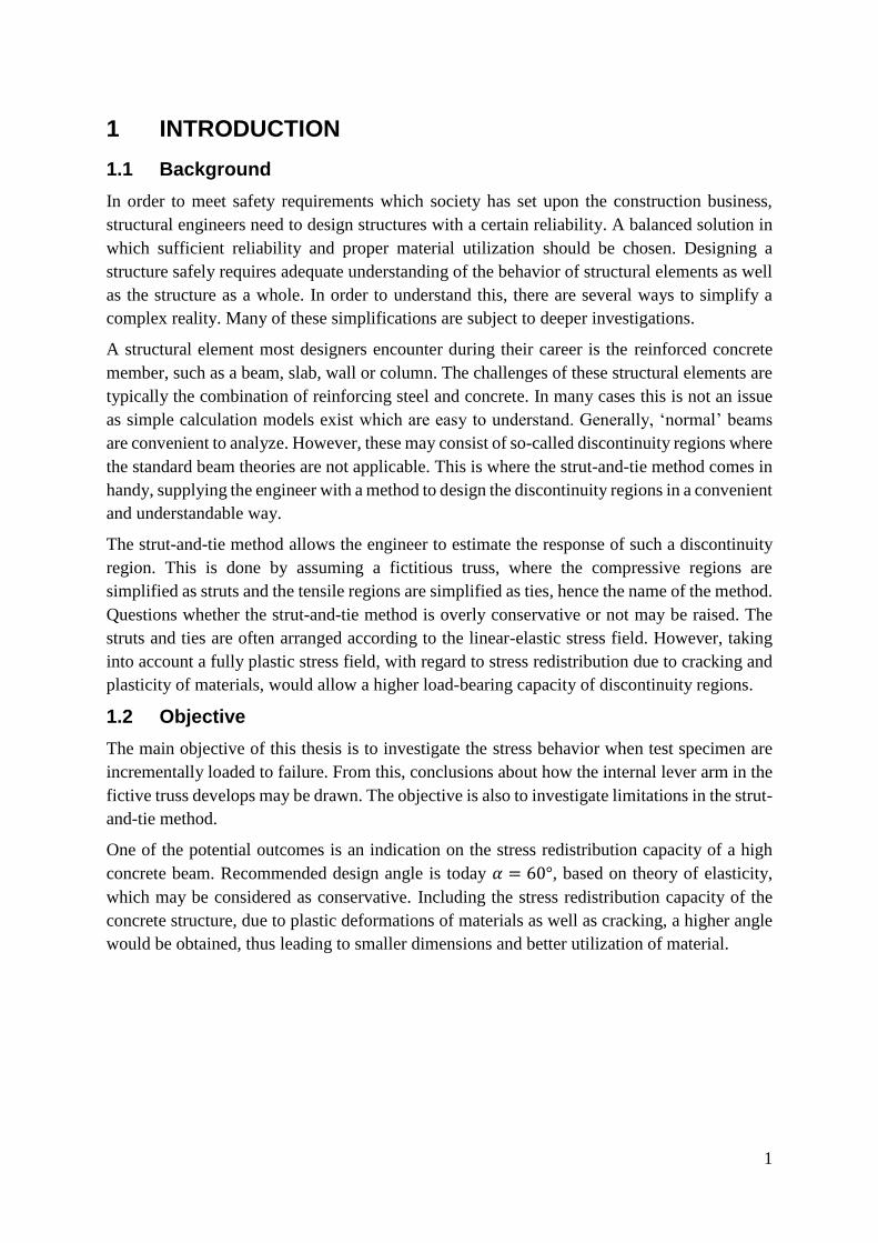
1.5 Tested model
The load case applied throughout this project is shown in Figure 1-1. The total load, F, applied
in the laboratory work will be divided into two point loads, more details in chapter 4. A
displacement-controlled loading was applied in the laboratory process. Thus, when modelling
in the finite element program BRIGADE/Plus the ‘forces’ were applied as displacements at the
top of the beam resulting in reaction forces in the supports, equal to the, forces on top according
to Newton’s third law [1]. Details concerning the computer modelling are presented in chapter
5.
Figure 1-1: Deformation and reaction forces
5
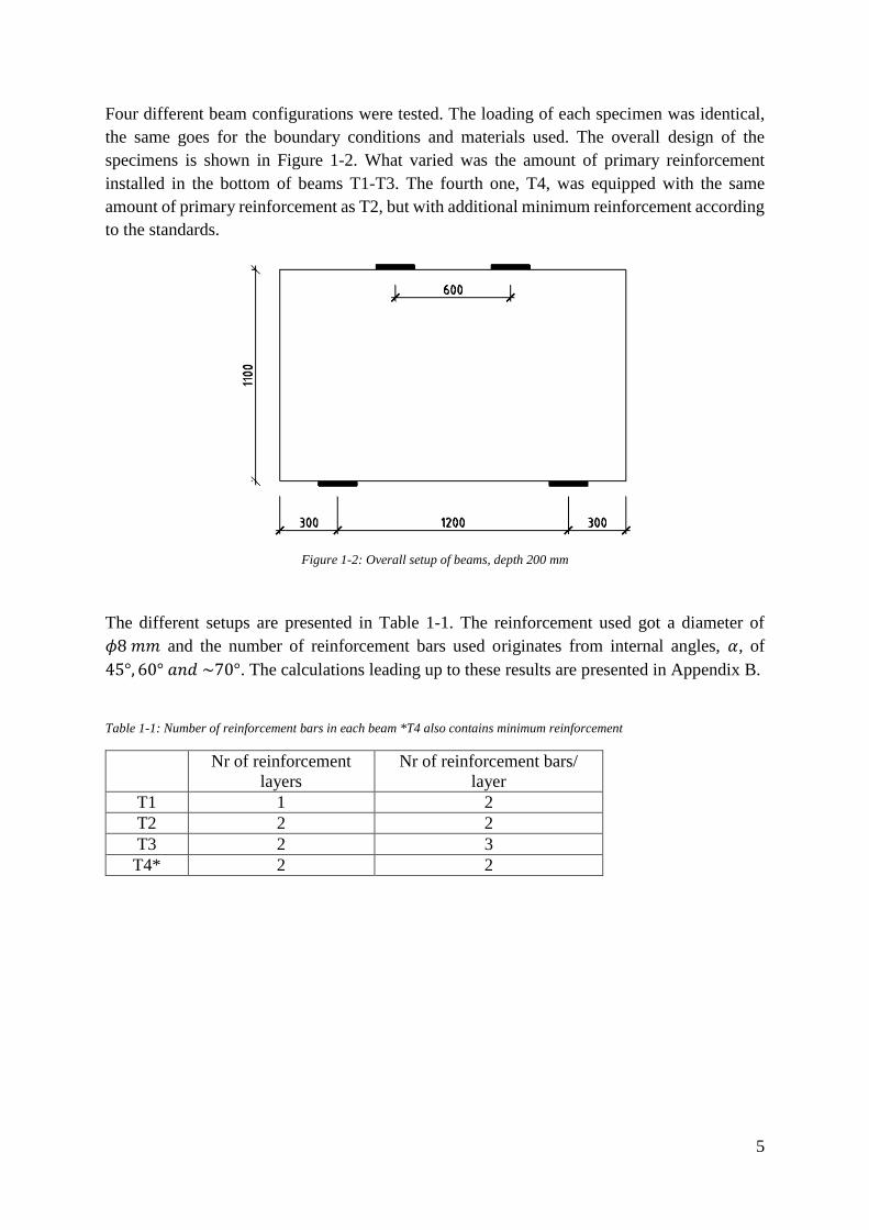
Four different beam configurations were tested. The loading of each specimen was identical,
the same goes for the boundary conditions and materials used. The overall design of the
specimens is shown in Figure 1-2. What varied was the amount of primary reinforcement
installed in the bottom of beams T1-T3. The fourth one, T4, was equipped with the same
amount of primary reinforcement as T2, but with additional minimum reinforcement according
to the standards.
Figure 1-2: Overall setup of beams, depth 200 mm
The different setups are presented in Table 1-1. The reinforcement used got a diameter of
𝜙8 𝑚𝑚 and the number of reinforcement bars used originates from internal angles, 𝛼, of
45°, 60° 𝑎𝑛𝑑 ~70°. The calculations leading up to these results are presented in Appendix B.
Table 1-1: Number of reinforcement bars in each beam *T4 also contains minimum reinforcement
Nr of reinforcement
layers
Nr of reinforcement bars/
layer
T1 1 2
T2 2 2
T3 2 3
T4* 2 2

6
7
2 BACKGROUND THEORY
The following chapter briefs the reader about some essential theory applied in the project. Some
basic beam theory together with properties of included materials is discussed. The strut-and-
tie method is explained, including its development as well as the hypothesis concerning the
internal angle from where this master thesis originate. Finally, constitutive modelling and
theoretical basis of the computer model is explained.
2.1 Materials
Beside the geometry, the most influential and obvious factor which contribute to the strength
and serviceability of a beam or bearing member, is the properties of the materials. The material
structure, their individual strength in tension and compression as well as their relationship to
each other and the collaboration between the different materials are decisive parts in a
structures load-bearing capacity. These parameters and the behavior is what will briefly be
explained in the following subsections.
2.1.1 Concrete
One commonly used building material is concrete, which is made up of cement, aggregates,
water and occasionally additives to obtain desired properties of the final product.
Concrete is a convenient building material to use because of its compressional strength and
versatility. Once a cast is made it is easy to pour the concrete, let it set and then make use of
the structure. A weakness of the material is its tensile strength - concrete has significantly
different behavior depending on how the load is applied. This fact makes it more complex to
analyze in terms of structural strength.
The difference between the materials anisotropic strengths is due to the fact of micro cracks in
the concrete, often in the face between the aggregate and the mortar, leaving the concrete
composite with a reduced tensile strength [2]. The solution to the low tensile strength is
reinforcement in the tensile areas, e.g. steel bars, subsection 2.1.3.
Furthermore, like many other materials, the behavior of the material is afflicted by the
multiaxial stress state, i.e. simultaneously stressing concrete in different directions will
severely affect the strength of the material.
8
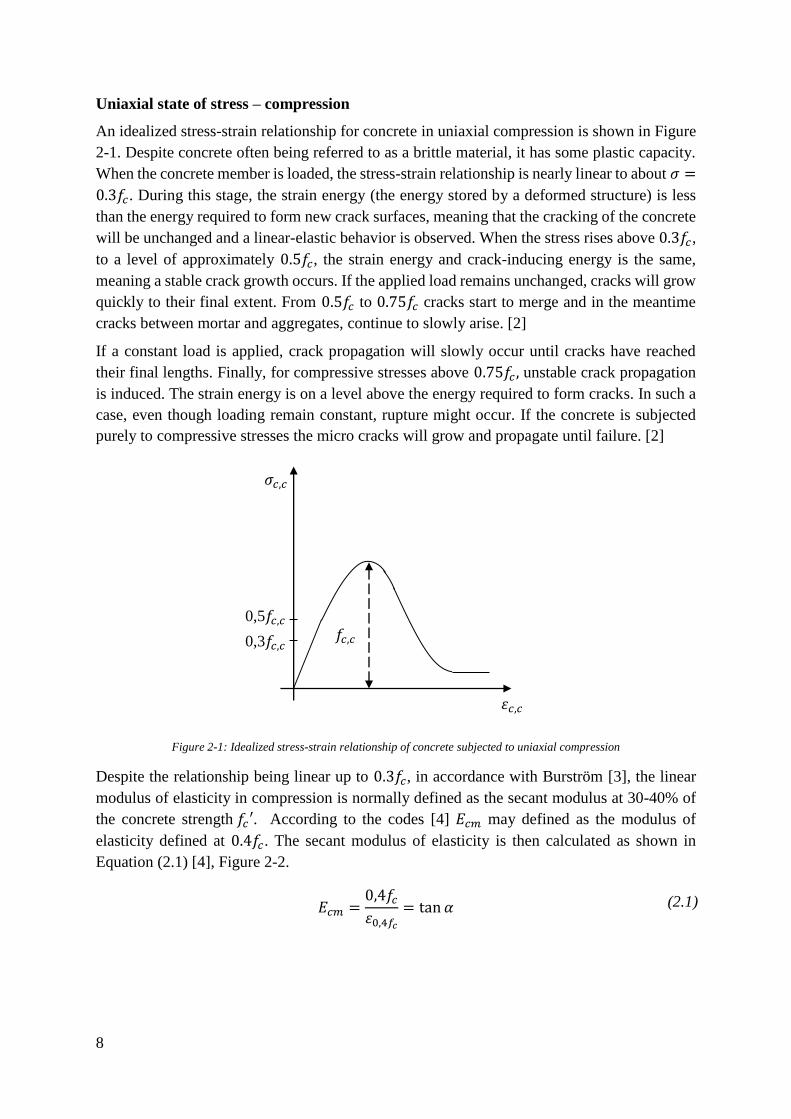
Uniaxial state of stress – compression
An idealized stress-strain relationship for concrete in uniaxial compression is shown in Figure
2-1. Despite concrete often being referred to as a brittle material, it has some plastic capacity.
When the concrete member is loaded, the stress-strain relationship is nearly linear to about 𝜎 =
0.3𝑓𝑐. During this stage, the strain energy (the energy stored by a deformed structure) is less
than the energy required to form new crack surfaces, meaning that the cracking of the concrete
will be unchanged and a linear-elastic behavior is observed. When the stress rises above 0.3𝑓𝑐,
to a level of approximately 0.5𝑓𝑐, the strain energy and crack-inducing energy is the same,
meaning a stable crack growth occurs. If the applied load remains unchanged, cracks will grow
quickly to their final extent. From 0.5𝑓𝑐 to 0.75𝑓𝑐 cracks start to merge and in the meantime
cracks between mortar and aggregates, continue to slowly arise. [2]
If a constant load is applied, crack propagation will slowly occur until cracks have reached
their final lengths. Finally, for compressive stresses above 0.75𝑓𝑐 , unstable crack propagation
is induced. The strain energy is on a level above the energy required to form cracks. In such a
case, even though loading remain constant, rupture might occur. If the concrete is subjected
purely to compressive stresses the micro cracks will grow and propagate until failure. [2]
Figure 2-1: Idealized stress-strain relationship of concrete subjected to uniaxial compression
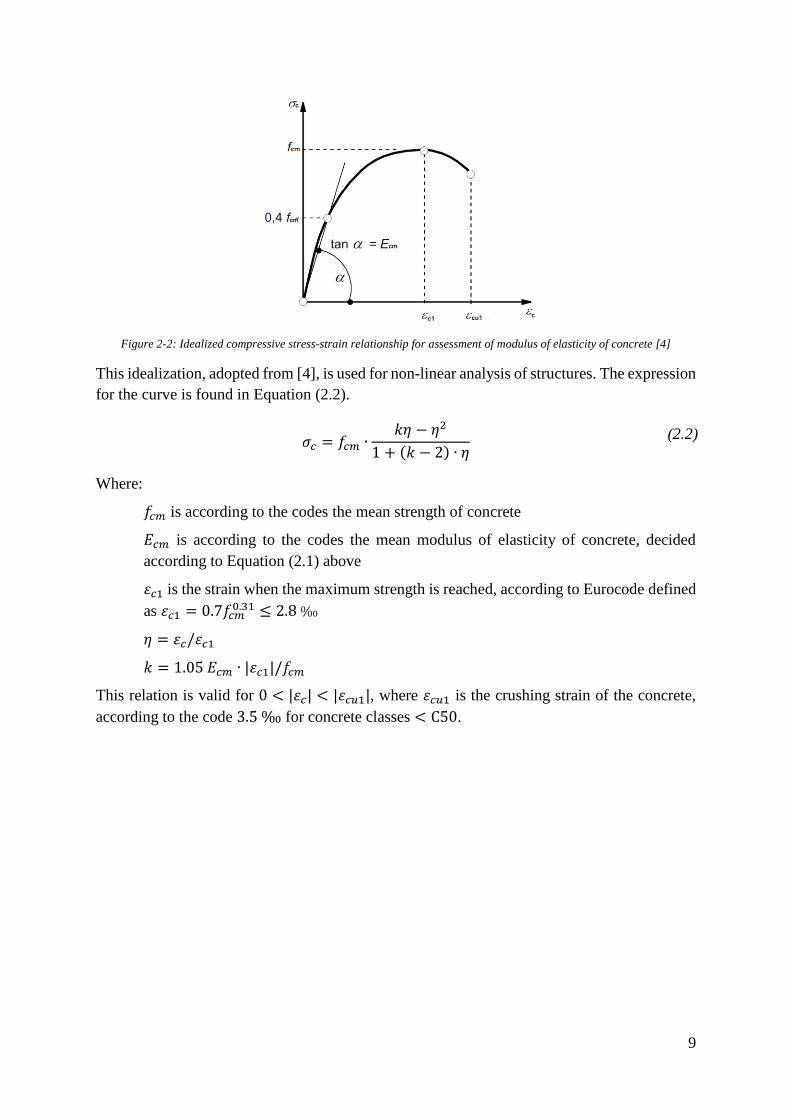
Despite the relationship being linear up to 0.3𝑓𝑐, in accordance with Burström [3], the linear
modulus of elasticity in compression is normally defined as the secant modulus at 30-40% of
the concrete strength 𝑓𝑐′. According to the codes [4] 𝐸𝑐𝑚 may defined as the modulus of
elasticity defined at 0.4𝑓𝑐. The secant modulus of elasticity is then calculated as shown in
Equation (2.1) [4], Figure 2-2.
𝐸𝑐𝑚 =
0,4𝑓𝑐
𝜀0,4𝑓𝑐
= tan 𝛼 (2.1)
𝜎𝑐,𝑐
𝜀𝑐,𝑐
𝑓𝑐,𝑐
0,3𝑓𝑐,𝑐
0,5𝑓𝑐,𝑐
9
Figure 2-2: Idealized compressive stress-strain relationship for assessment of modulus of elasticity of concrete [4]
This idealization, adopted from [4], is used for non-linear analysis of structures. The expression
for the curve is found in Equation (2.2).
𝜎𝑐 = 𝑓𝑐𝑚 ∙
𝑘𝜂 − 𝜂2
1 + (𝑘 − 2) ∙ 𝜂
(2.2)
Where:
𝑓𝑐𝑚 is according to the codes the mean strength of concrete
𝐸𝑐𝑚 is according to the codes the mean modulus of elasticity of concrete, decided
according to Equation (2.1) above
𝜀𝑐1 is the strain when the maximum strength is reached, according to Eurocode defined
as 𝜀𝑐1 = 0.7𝑓𝑐𝑚0.31 ≤ 2.8 ‰
𝜂 = 𝜀𝑐/𝜀𝑐1
𝑘 = 1.05 𝐸𝑐𝑚 ∙ |𝜀𝑐1|/𝑓𝑐𝑚
This relation is valid for 0 < |𝜀𝑐| < |𝜀𝑐𝑢1|, where 𝜀𝑐𝑢1 is the crushing strain of the concrete,
according to the code 3.5 ‰ for concrete classes < C50.
10
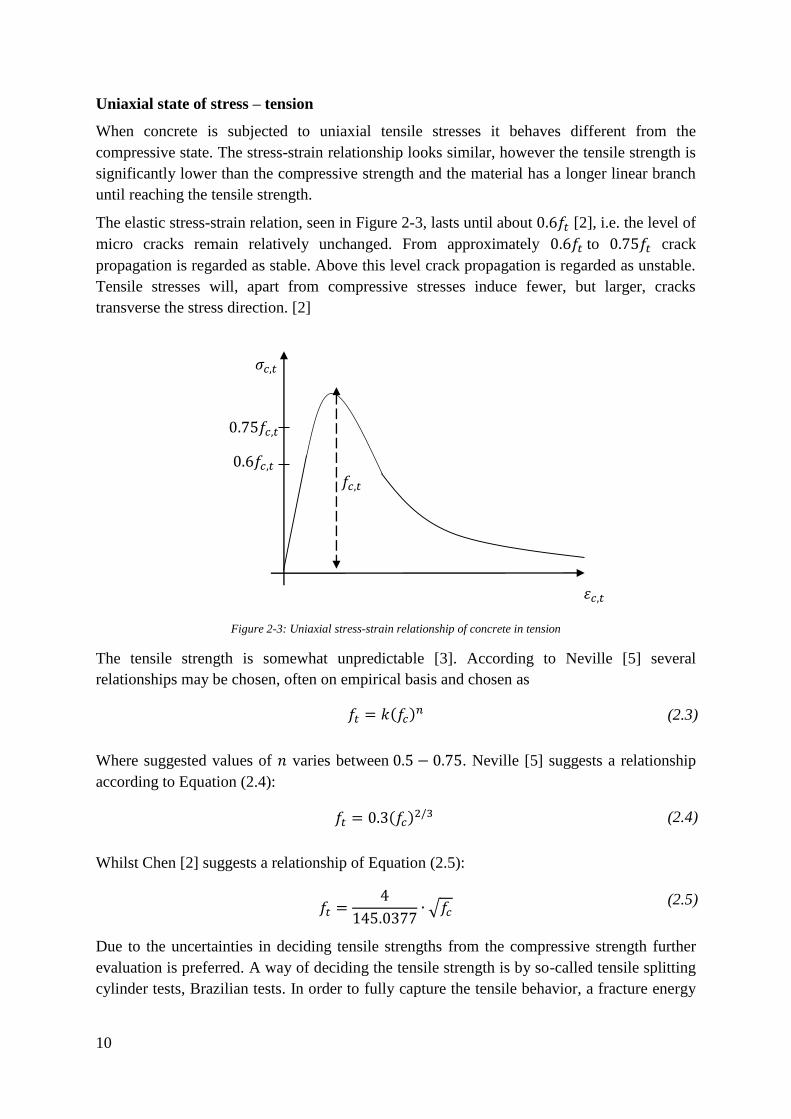
Uniaxial state of stress – tension
When concrete is subjected to uniaxial tensile stresses it behaves different from the
compressive state. The stress-strain relationship looks similar, however the tensile strength is
significantly lower than the compressive strength and the material has a longer linear branch
until reaching the tensile strength.
The elastic stress-strain relation, seen in Figure 2-3, lasts until about 0.6𝑓𝑡 [2], i.e. the level of
micro cracks remain relatively unchanged. From approximately 0.6𝑓𝑡 to 0.75𝑓𝑡 crack
propagation is regarded as stable. Above this level crack propagation is regarded as unstable.
Tensile stresses will, apart from compressive stresses induce fewer, but larger, cracks
transverse the stress direction. [2]
Figure 2-3: Uniaxial stress-strain relationship of concrete in tension
The tensile strength is somewhat unpredictable [3]. According to Neville [5] several
relationships may be chosen, often on empirical basis and chosen as
𝑓𝑡 = 𝑘(𝑓𝑐)𝑛 (2.3)
Where suggested values of 𝑛 varies between 0.5 − 0.75. Neville [5] suggests a relationship
according to Equation (2.4):
𝑓𝑡 = 0.3(𝑓𝑐)2/3 (2.4)
Whilst Chen [2] suggests a relationship of Equation (2.5):
𝑓𝑡 =
4
145.0377∙ √𝑓𝑐
(2.5)
Due to the uncertainties in deciding tensile strengths from the compressive strength further
evaluation is preferred. A way of deciding the tensile strength is by so-called tensile splitting
cylinder tests, Brazilian tests. In order to fully capture the tensile behavior, a fracture energy
𝜎𝑐,𝑡
𝜀𝑐,𝑡
𝑓𝑐,𝑡
0.75𝑓𝑐,𝑡
0.6𝑓𝑐,𝑡
11
criterion is complementing the pure tensile strength. This fracture energy criterion is explained
in subsection 0. Tests of the material properties are described in subsection 4.1.1.
Biaxial state of stress
A concrete member subjected to a biaxial stress state will have an impact on its behavior. Due
to the different response from tensile and compressive stresses, differences exists whether the
member is under compressive-compressive (CC), compressive-tensile (CT) or tensile-tensile
stresses (TT) [2]. Generally, a CC-stress state yields a higher strength than uniaxial
compressive strength, a CT-stress state a lower strength than uniaxial compressive strength and
a TT-state a lower or approximately same strength compared to uniaxial tensile strength.
12
2.1.2 Reinforcing Steel
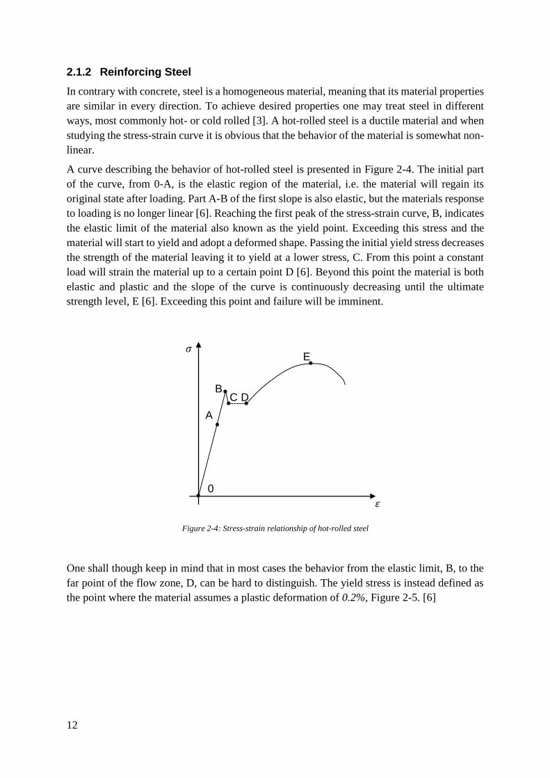
In contrary with concrete, steel is a homogeneous material, meaning that its material properties
are similar in every direction. To achieve desired properties one may treat steel in different
ways, most commonly hot- or cold rolled [3]. A hot-rolled steel is a ductile material and when
studying the stress-strain curve it is obvious that the behavior of the material is somewhat non-
linear.
A curve describing the behavior of hot-rolled steel is presented in Figure 2-4. The initial part
of the curve, from 0-A, is the elastic region of the material, i.e. the material will regain its
original state after loading. Part A-B of the first slope is also elastic, but the materials response
to loading is no longer linear [6]. Reaching the first peak of the stress-strain curve, B, indicates
the elastic limit of the material also known as the yield point. Exceeding this stress and the
material will start to yield and adopt a deformed shape. Passing the initial yield stress decreases
the strength of the material leaving it to yield at a lower stress, C. From this point a constant
load will strain the material up to a certain point D [6]. Beyond this point the material is both
elastic and plastic and the slope of the curve is continuously decreasing until the ultimate
strength level, E [6]. Exceeding this point and failure will be imminent.
Figure 2-4: Stress-strain relationship of hot-rolled steel
One shall though keep in mind that in most cases the behavior from the elastic limit, B, to the
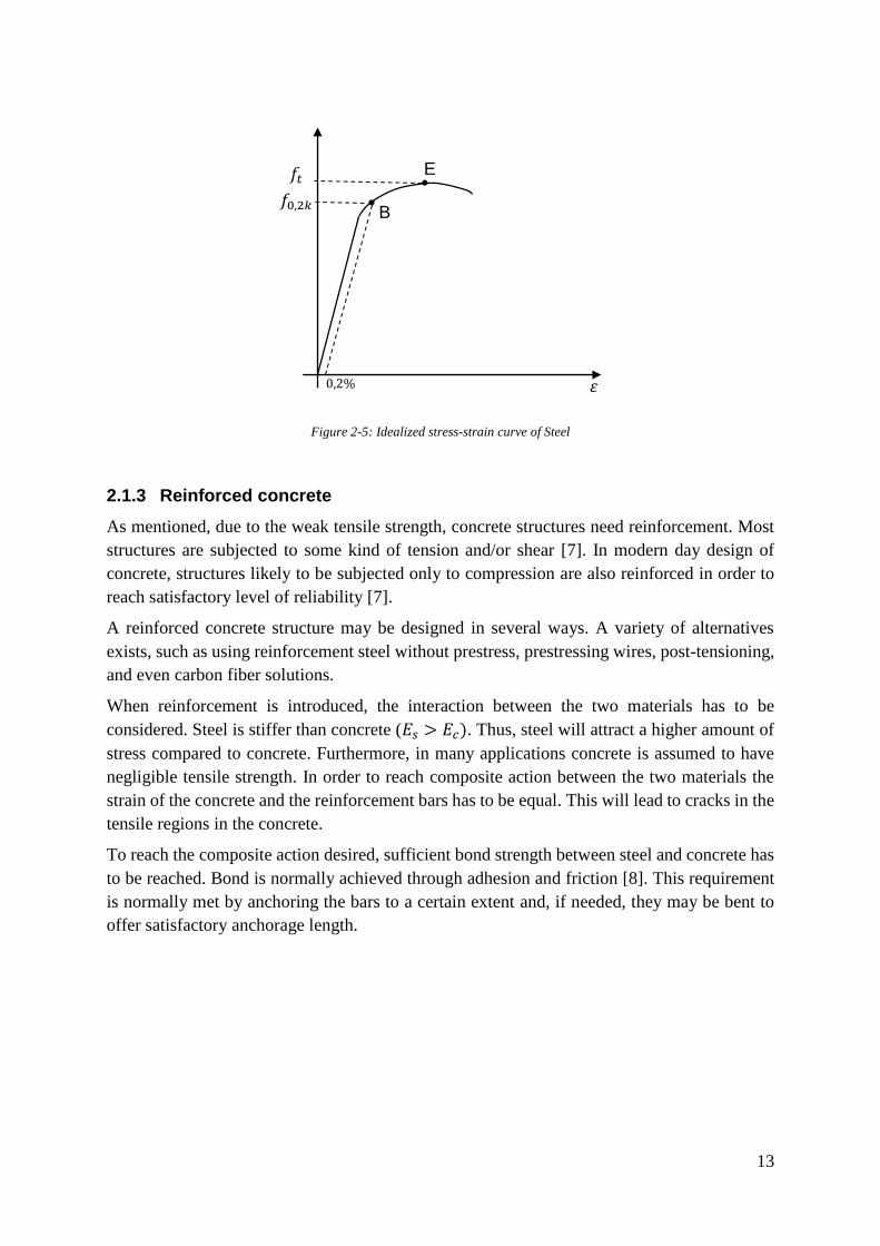
far point of the flow zone, D, can be hard to distinguish. The yield stress is instead defined as
the point where the material assumes a plastic deformation of 0.2%, Figure 2-5. [6]
A
B C D
E 𝜎
𝜀
0
13
Figure 2-5: Idealized stress-strain curve of Steel
2.1.3 Reinforced concrete
As mentioned, due to the weak tensile strength, concrete structures need reinforcement. Most
structures are subjected to some kind of tension and/or shear [7]. In modern day design of
concrete, structures likely to be subjected only to compression are also reinforced in order to
reach satisfactory level of reliability [7].
A reinforced concrete structure may be designed in several ways. A variety of alternatives
exists, such as using reinforcement steel without prestress, prestressing wires, post-tensioning,
and even carbon fiber solutions.
When reinforcement is introduced, the interaction between the two materials has to be
considered. Steel is stiffer than concrete (𝐸𝑠 > 𝐸𝑐). Thus, steel will attract a higher amount of
stress compared to concrete. Furthermore, in many applications concrete is assumed to have
negligible tensile strength. In order to reach composite action between the two materials the
strain of the concrete and the reinforcement bars has to be equal. This will lead to cracks in the
tensile regions in the concrete.
To reach the composite action desired, sufficient bond strength between steel and concrete has
to be reached. Bond is normally achieved through adhesion and friction [8]. This requirement
is normally met by anchoring the bars to a certain extent and, if needed, they may be bent to
offer satisfactory anchorage length.
E
𝜀
B
0,2%
𝑓0,2𝑘
𝑓𝑡
14
2.2 Stress distribution
This section briefly discusses the stresses within a structure subjected to a load.
2.2.1 Linear stress distribution
In basic beam theory, also known as Bernoulli-Euler beam theory, it is often assumed that plane
sections remain plane, sections remain perpendicular to its center line and that the strains varies
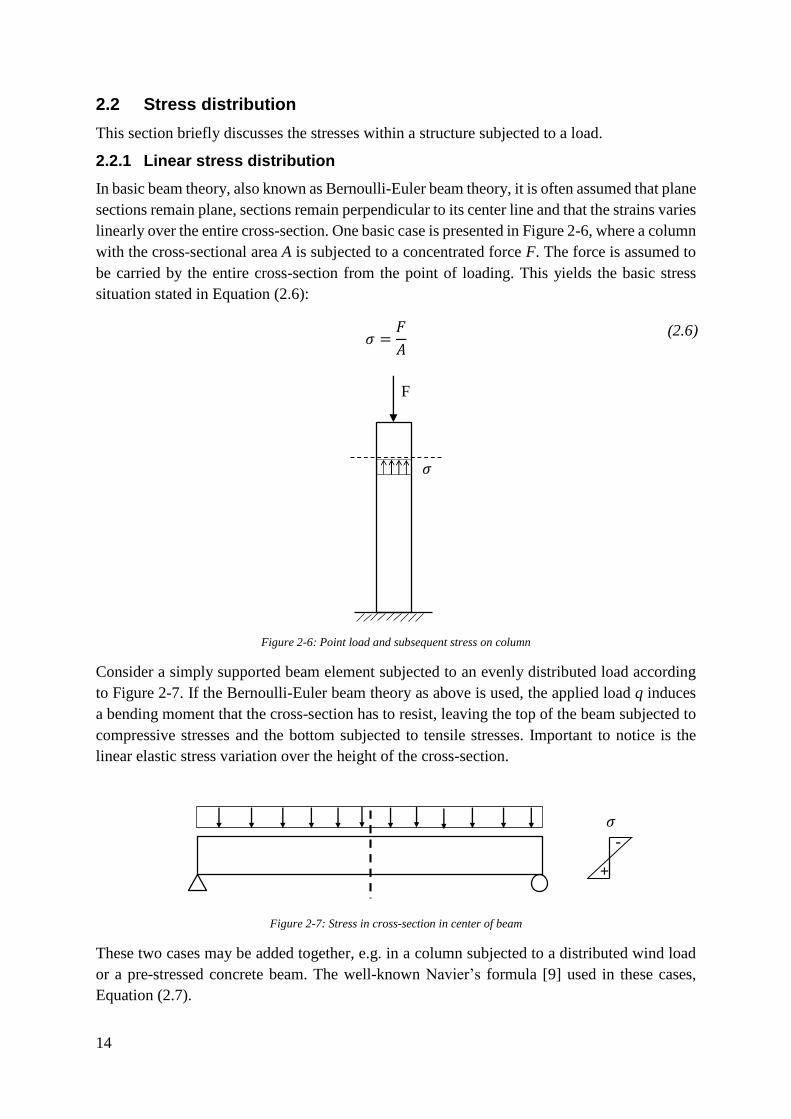
linearly over the entire cross-section. One basic case is presented in Figure 2-6, where a column
with the cross-sectional area A is subjected to a concentrated force F. The force is assumed to
be carried by the entire cross-section from the point of loading. This yields the basic stress
situation stated in Equation (2.6):
𝜎 =
𝐹
𝐴
(2.6)
Figure 2-6: Point load and subsequent stress on column
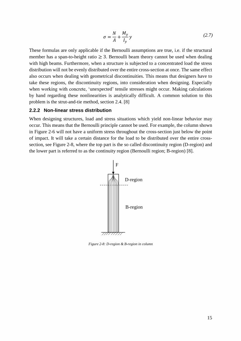
Consider a simply supported beam element subjected to an evenly distributed load according
to Figure 2-7. If the Bernoulli-Euler beam theory as above is used, the applied load q induces
a bending moment that the cross-section has to resist, leaving the top of the beam subjected to
compressive stresses and the bottom subjected to tensile stresses. Important to notice is the
linear elastic stress variation over the height of the cross-section.
Figure 2-7: Stress in cross-section in center of beam
These two cases may be added together, e.g. in a column subjected to a distributed wind load
or a pre-stressed concrete beam. The well-known Navier’s formula [9] used in these cases,
Equation (2.7).
F
𝜎
+
-
𝜎
15
𝜎 =
𝑁
𝐴+
𝑀𝑦
𝐼𝑦𝑦 (2.7)
These formulas are only applicable if the Bernoulli assumptions are true, i.e. if the structural
member has a span-to-height ratio ≥ 3. Bernoulli beam theory cannot be used when dealing
with high beams. Furthermore, when a structure is subjected to a concentrated load the stress
distribution will not be evenly distributed over the entire cross-section at once. The same effect
also occurs when dealing with geometrical discontinuities. This means that designers have to
take these regions, the discontinuity regions, into consideration when designing. Especially
when working with concrete, ‘unexpected’ tensile stresses might occur. Making calculations
by hand regarding these nonlinearities is analytically difficult. A common solution to this
problem is the strut-and-tie method, section 2.4. [8]
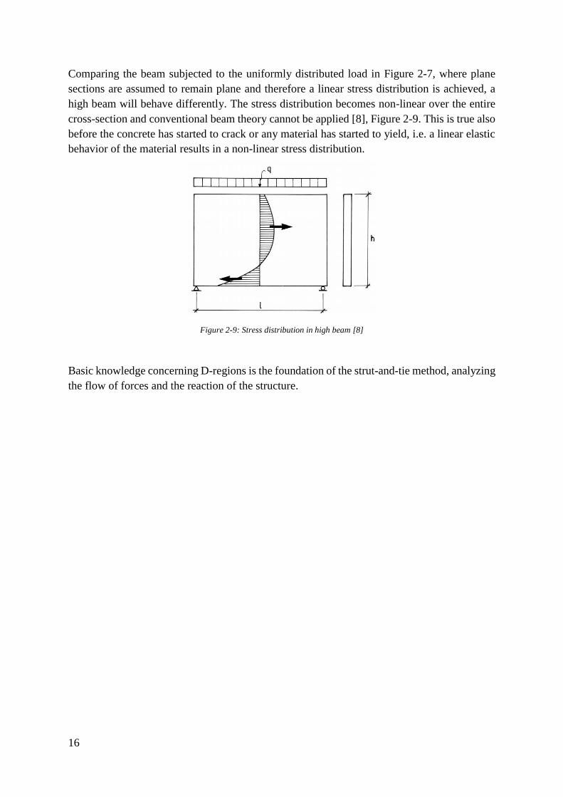
2.2.2 Non-linear stress distribution
When designing structures, load and stress situations which yield non-linear behavior may
occur. This means that the Bernoulli principle cannot be used. For example, the column shown
in Figure 2-6 will not have a uniform stress throughout the cross-section just below the point
of impact. It will take a certain distance for the load to be distributed over the entire cross-
section, see Figure 2-8, where the top part is the so called discontinuity region (D-region) and
the lower part is referred to as the continuity region (Bernoulli region; B-region) [8].
Figure 2-8: D-region & B-region in column
F
D-region
B-region
16
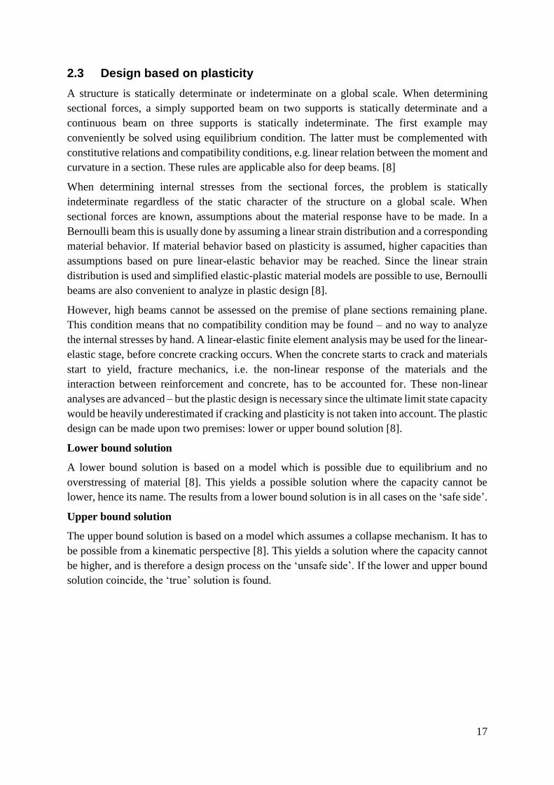
Comparing the beam subjected to the uniformly distributed load in Figure 2-7, where plane
sections are assumed to remain plane and therefore a linear stress distribution is achieved, a
high beam will behave differently. The stress distribution becomes non-linear over the entire
cross-section and conventional beam theory cannot be applied [8], Figure 2-9. This is true also
before the concrete has started to crack or any material has started to yield, i.e. a linear elastic
behavior of the material results in a non-linear stress distribution.
Figure 2-9: Stress distribution in high beam [8]
Basic knowledge concerning D-regions is the foundation of the strut-and-tie method, analyzing
the flow of forces and the reaction of the structure.
17
2.3 Design based on plasticity
A structure is statically determinate or indeterminate on a global scale. When determining
sectional forces, a simply supported beam on two supports is statically determinate and a
continuous beam on three supports is statically indeterminate. The first example may
conveniently be solved using equilibrium condition. The latter must be complemented with
constitutive relations and compatibility conditions, e.g. linear relation between the moment and
curvature in a section. These rules are applicable also for deep beams. [8]
When determining internal stresses from the sectional forces, the problem is statically
indeterminate regardless of the static character of the structure on a global scale. When
sectional forces are known, assumptions about the material response have to be made. In a
Bernoulli beam this is usually done by assuming a linear strain distribution and a corresponding
material behavior. If material behavior based on plasticity is assumed, higher capacities than
assumptions based on pure linear-elastic behavior may be reached. Since the linear strain
distribution is used and simplified elastic-plastic material models are possible to use, Bernoulli
beams are also convenient to analyze in plastic design [8].
However, high beams cannot be assessed on the premise of plane sections remaining plane.
This condition means that no compatibility condition may be found – and no way to analyze
the internal stresses by hand. A linear-elastic finite element analysis may be used for the linear-
elastic stage, before concrete cracking occurs. When the concrete starts to crack and materials
start to yield, fracture mechanics, i.e. the non-linear response of the materials and the
interaction between reinforcement and concrete, has to be accounted for. These non-linear
analyses are advanced – but the plastic design is necessary since the ultimate limit state capacity
would be heavily underestimated if cracking and plasticity is not taken into account. The plastic
design can be made upon two premises: lower or upper bound solution [8].
Lower bound solution
A lower bound solution is based on a model which is possible due to equilibrium and no
overstressing of material [8]. This yields a possible solution where the capacity cannot be
lower, hence its name. The results from a lower bound solution is in all cases on the ‘safe side’.
Upper bound solution
The upper bound solution is based on a model which assumes a collapse mechanism. It has to
be possible from a kinematic perspective [8]. This yields a solution where the capacity cannot
be higher, and is therefore a design process on the ‘unsafe side’. If the lower and upper bound
solution coincide, the ‘true’ solution is found.
18
2.4 The strut-and-tie method
Solving the complexities of discontinuity regions, described in subsection 2.2.2 and section
2.3, can be made using the strut-and-tie method in the ultimate limit state (ULS). The
discontinuity regions may occur close to concentrated loads or geometrical discontinuities.
These regions extends approximately as far as the width of the cross-section, often making the
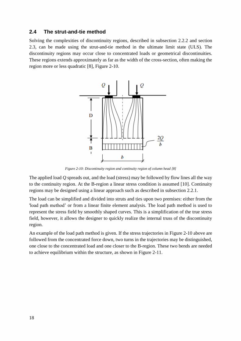
region more or less quadratic [8], Figure 2-10.
Figure 2-10: Discontinuity region and continuity region of column head [8]
The applied load Q spreads out, and the load (stress) may be followed by flow lines all the way
to the continuity region. At the B-region a linear stress condition is assumed [10]. Continuity
regions may be designed using a linear approach such as described in subsection 2.2.1.
The load can be simplified and divided into struts and ties upon two premises: either from the
'load path method’ or from a linear finite element analysis. The load path method is used to
represent the stress field by smoothly shaped curves. This is a simplification of the true stress
field, however, it allows the designer to quickly realize the internal truss of the discontinuity
region.
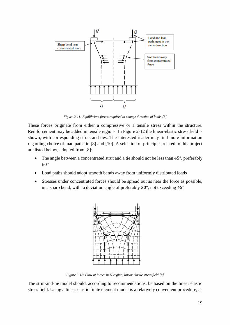
An example of the load path method is given. If the stress trajectories in Figure 2-10 above are
followed from the concentrated force down, two turns in the trajectories may be distinguished,
one close to the concentrated load and one closer to the B-region. These two bends are needed
to achieve equilibrium within the structure, as shown in Figure 2-11.
19
Figure 2-11: Equilibrium forces required to change direction of loads [8]
These forces originate from either a compressive or a tensile stress within the structure.
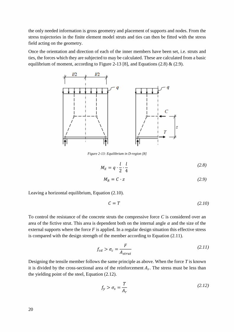
Reinforcement may be added in tensile regions. In Figure 2-12 the linear-elastic stress field is
shown, with corresponding struts and ties. The interested reader may find more information
regarding choice of load paths in [8] and [10]. A selection of principles related to this project
are listed below, adopted from [8]:
The angle between a concentrated strut and a tie should not be less than 45°, preferably
60°
Load paths should adopt smooth bends away from uniformly distributed loads
Stresses under concentrated forces should be spread out as near the force as possible,
in a sharp bend, with a deviation angle of preferably 30°, not exceeding 45°
Figure 2-12: Flow of forces in D-region, linear-elastic stress field [8]
The strut-and-tie model should, according to recommendations, be based on the linear elastic
stress field. Using a linear elastic finite element model is a relatively convenient procedure, as
20
the only needed information is gross geometry and placement of supports and nodes. From the
stress trajectories in the finite element model struts and ties can then be fitted with the stress
field acting on the geometry.
Once the orientation and direction of each of the inner members have been set, i.e. struts and
ties, the forces which they are subjected to may be calculated. These are calculated from a basic
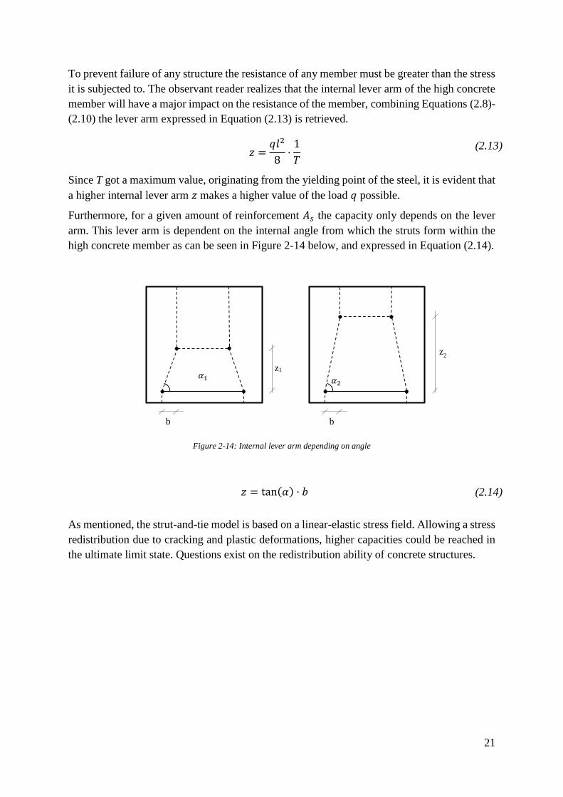
equilibrium of moment, according to Figure 2-13 [8], and Equations (2.8) & (2.9).
Figure 2-13: Equilibrium in D-region [8]
𝑀𝐸 = 𝑞 ·
𝑙
2·
𝑙
4
(2.8)
𝑀𝑅 = 𝐶 · 𝑧 (2.9)
Leaving a horizontal equilibrium, Equation (2.10).
𝐶 = 𝑇 (2.10)
To control the resistance of the concrete struts the compressive force C is considered over an
area of the fictive strut. This area is dependent both on the internal angle 𝛼 and the size of the
external supports where the force F is applied. In a regular design situation this effective stress
is compared with the design strength of the member according to Equation (2.11).
𝑓𝑐𝑑 > 𝜎𝑐 =
𝐹
𝐴𝑠𝑡𝑟𝑢𝑡 (2.11)
Designing the tensile member follows the same principle as above. When the force T is known
it is divided by the cross-sectional area of the reinforcement 𝐴𝑟. The stress must be less than
the yielding point of the steel, Equation (2.12).
𝑓𝑦 > 𝜎𝑠 =
𝑇
𝐴𝑟 (2.12)
21
To prevent failure of any structure the resistance of any member must be greater than the stress
it is subjected to. The observant reader realizes that the internal lever arm of the high concrete
member will have a major impact on the resistance of the member, combining Equations (2.8)-
(2.10) the lever arm expressed in Equation (2.13) is retrieved.
𝑧 =
𝑞𝑙2
8·
1
𝑇
(2.13)
Since T got a maximum value, originating from the yielding point of the steel, it is evident that
a higher internal lever arm 𝑧 makes a higher value of the load 𝑞 possible.
Furthermore, for a given amount of reinforcement 𝐴𝑠 the capacity only depends on the lever
arm. This lever arm is dependent on the internal angle from which the struts form within the
high concrete member as can be seen in Figure 2-14 below, and expressed in Equation (2.14).
Figure 2-14: Internal lever arm depending on angle
𝑧 = tan(𝛼) · 𝑏 (2.14)
As mentioned, the strut-and-tie model is based on a linear-elastic stress field. Allowing a stress
redistribution due to cracking and plastic deformations, higher capacities could be reached in
the ultimate limit state. Questions exist on the redistribution ability of concrete structures.
b
𝛼1
z1
b
𝛼2
z2
22
2.4.1 Examples of applications of the strut-and-tie method
The strut-and-tie approach can be applied in cases other than high beams. A few examples will
be given in this subsection to present the widespread usage of the method.
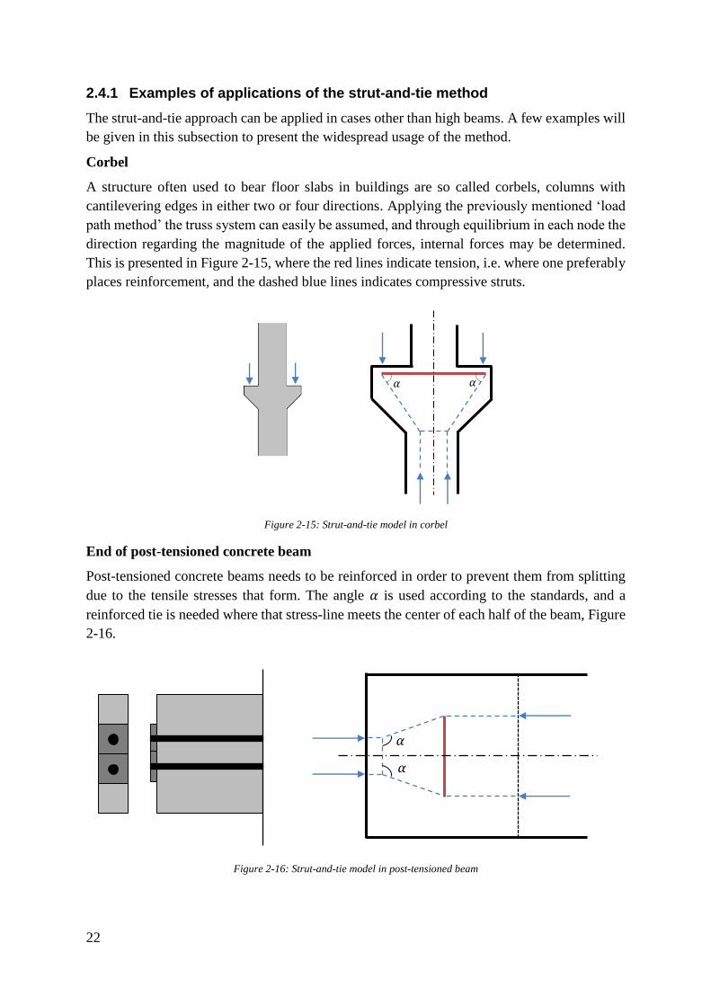
Corbel
A structure often used to bear floor slabs in buildings are so called corbels, columns with
cantilevering edges in either two or four directions. Applying the previously mentioned ‘load
path method’ the truss system can easily be assumed, and through equilibrium in each node the
direction regarding the magnitude of the applied forces, internal forces may be determined.
This is presented in Figure 2-15, where the red lines indicate tension, i.e. where one preferably
places reinforcement, and the dashed blue lines indicates compressive struts.
Figure 2-15: Strut-and-tie model in corbel
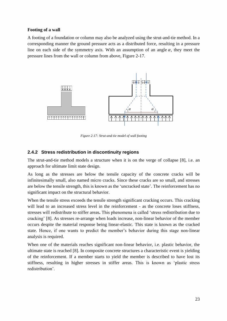
End of post-tensioned concrete beam
Post-tensioned concrete beams needs to be reinforced in order to prevent them from splitting
due to the tensile stresses that form. The angle 𝛼 is used according to the standards, and a
reinforced tie is needed where that stress-line meets the center of each half of the beam, Figure
2-16.
Figure 2-16: Strut-and-tie model in post-tensioned beam
𝛼 𝛼
𝛼
𝛼
23
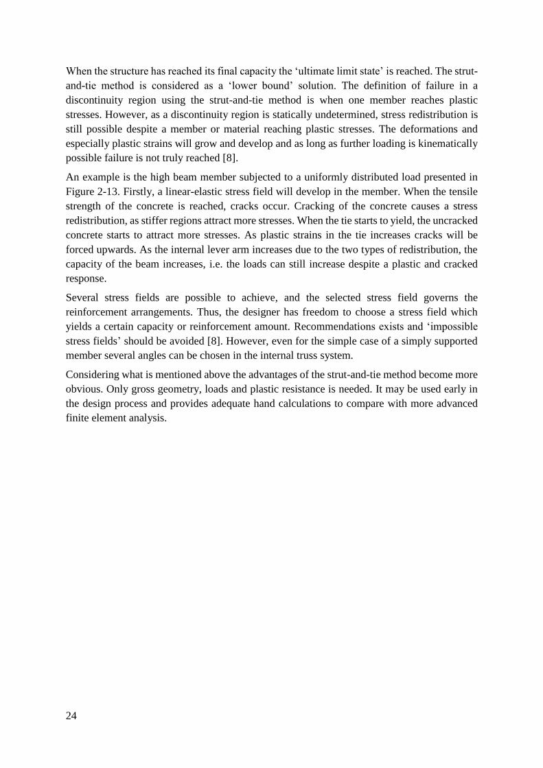
Footing of a wall
A footing of a foundation or column may also be analyzed using the strut-and-tie method. In a
corresponding manner the ground pressure acts as a distributed force, resulting in a pressure
line on each side of the symmetry axis. With an assumption of an angle 𝛼, they meet the
pressure lines from the wall or column from above, Figure 2-17.
Figure 2-17: Strut-and-tie model of wall footing
2.4.2 Stress redistribution in discontinuity regions
The strut-and-tie method models a structure when it is on the verge of collapse [8], i.e. an
approach for ultimate limit state design.
As long as the stresses are below the tensile capacity of the concrete cracks will be
infinitesimally small, also named micro cracks. Since these cracks are so small, and stresses
are below the tensile strength, this is known as the ‘uncracked state’. The reinforcement has no
significant impact on the structural behavior.
When the tensile stress exceeds the tensile strength significant cracking occurs. This cracking
will lead to an increased stress level in the reinforcement - as the concrete loses stiffness,
stresses will redistribute to stiffer areas. This phenomena is called ‘stress redistribution due to
cracking’ [8]. As stresses re-arrange when loads increase, non-linear behavior of the member
occurs despite the material response being linear-elastic. This state is known as the cracked
state. Hence, if one wants to predict the member’s behavior during this stage non-linear
analysis is required.
When one of the materials reaches significant non-linear behavior, i.e. plastic behavior, the
ultimate state is reached [8]. In composite concrete structures a characteristic event is yielding
of the reinforcement. If a member starts to yield the member is described to have lost its
stiffness, resulting in higher stresses in stiffer areas. This is known as ‘plastic stress
redistribution’.
𝛼 𝛼
24
When the structure has reached its final capacity the ‘ultimate limit state’ is reached. The strut-
and-tie method is considered as a ‘lower bound’ solution. The definition of failure in a
discontinuity region using the strut-and-tie method is when one member reaches plastic
stresses. However, as a discontinuity region is statically undetermined, stress redistribution is
still possible despite a member or material reaching plastic stresses. The deformations and
especially plastic strains will grow and develop and as long as further loading is kinematically
possible failure is not truly reached [8].
An example is the high beam member subjected to a uniformly distributed load presented in
Figure 2-13. Firstly, a linear-elastic stress field will develop in the member. When the tensile
strength of the concrete is reached, cracks occur. Cracking of the concrete causes a stress
redistribution, as stiffer regions attract more stresses. When the tie starts to yield, the uncracked
concrete starts to attract more stresses. As plastic strains in the tie increases cracks will be
forced upwards. As the internal lever arm increases due to the two types of redistribution, the
capacity of the beam increases, i.e. the loads can still increase despite a plastic and cracked
response.
Several stress fields are possible to achieve, and the selected stress field governs the
reinforcement arrangements. Thus, the designer has freedom to choose a stress field which
yields a certain capacity or reinforcement amount. Recommendations exists and ‘impossible
stress fields’ should be avoided [8]. However, even for the simple case of a simply supported
member several angles can be chosen in the internal truss system.
Considering what is mentioned above the advantages of the strut-and-tie method become more
obvious. Only gross geometry, loads and plastic resistance is needed. It may be used early in
the design process and provides adequate hand calculations to compare with more advanced
finite element analysis.
25
2.5 Risk assessment and safety factors
Usually when designing a structure characteristic strength values are used for the members
included to assure a safe structure, i.e., the real strength has a probability of 95% to be higher
than the one assumed in the design process. The strength of the members is assumed to be
normally distributed.
In the same manner the load applied is often assumed to be in the top 2%, leaving an acceptable
level of probability of failure.
However in this project the mean strength is used when the primary calculations are made. The
reason for this is the laboratory testing process where it is most likely to receive strength values
close to the mean strength.
Safety factors are normally used when designing structures to provide an acceptable probability
of failure. When the primary calculations were made the authors were looking for a certain
type of failure to clearly show the ‘strut-and-tie behavior’. This means that safety factors were
used when designing struts, nodes and reinforcement anchorage lengths to prevent undesirable
failures, but not when the ties were designed.
In practice, the following relations are used in this project when calculations have been made
(Equation (2.15)-(2.18)):
𝑓𝑐𝑑 =
𝑓𝑐𝑚
𝛾𝐶 (2.15)
𝑓𝑐𝑚 = 𝑓𝑐𝑘 + 8 [𝑀𝑃𝑎] (2.16)
𝑓𝑐𝑡,𝑑 =
𝑓𝑐𝑡𝑚
𝛾𝐶 (2.17)
𝑓𝑦𝑑 = 𝑓𝑦𝑘 (2.18)
26
2.6 Finite element model
The program used, BRIGADE/Plus, is a finite element software. Dividing a defined structure
into a number of smaller numerical part, i.e. finite elements, simulations can be performed over
the region. Nonlinear behavior of an entire structure may be considered linearly within each
small element, all of these elements together is called a finite element mesh [11]. The
simulations are stated as numerical approximations of differential equations, and each element
effect the behavior of its neighbors, leading to increased number of calculations depending on
the size of the structure and how coarse of a mesh is used [11].
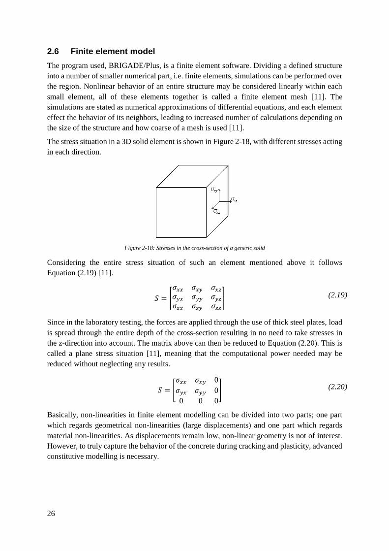
The stress situation in a 3D solid element is shown in Figure 2-18, with different stresses acting
in each direction.
Figure 2-18: Stresses in the cross-section of a generic solid
Considering the entire stress situation of such an element mentioned above it follows
Equation (2.19) [11].
𝑆 = [
𝜎𝑥𝑥 𝜎𝑥𝑦 𝜎𝑥𝑧
𝜎𝑦𝑥 𝜎𝑦𝑦 𝜎𝑦𝑧
𝜎𝑧𝑥 𝜎𝑧𝑦 𝜎𝑧𝑧
] (2.19)
Since in the laboratory testing, the forces are applied through the use of thick steel plates, load
is spread through the entire depth of the cross-section resulting in no need to take stresses in
the z-direction into account. The matrix above can then be reduced to Equation (2.20). This is
called a plane stress situation [11], meaning that the computational power needed may be
reduced without neglecting any results.
𝑆 = [
𝜎𝑥𝑥 𝜎𝑥𝑦 0
𝜎𝑦𝑥 𝜎𝑦𝑦 0
0 0 0
] (2.20)
Basically, non-linearities in finite element modelling can be divided into two parts; one part
which regards geometrical non-linearities (large displacements) and one part which regards
material non-linearities. As displacements remain low, non-linear geometry is not of interest.
However, to truly capture the behavior of the concrete during cracking and plasticity, advanced
constitutive modelling is necessary.
27
2.6.1 Constitutive modeling using Concrete Damaged Plasticity model
In order to capture the behavior of the stress redistribution due to cracking and plasticity, the
model has to consider some advanced theory; plasticity, damage theory and fracture mechanics.
Plasticity in terms of pure material behavior has been presented in sections above. The
constitutive model used is the Concrete Damaged Plasticity model.
Fracture mechanics
As the strut-and-tie method takes into account plastic redistribution due to cracking, cracking
has to be considered when modelling, using fracture mechanics. In this project non-linear
fracture mechanics was used. However to provide the reader with a more thorough
understanding the more convenient linear elastic case is presented initially. Conventional
fracture mechanics requires an existing crack, whereas fracture mechanics used in the Concrete
Damaged Plasticity model does not.
In conventional fracture mechanics stresses and strains are assumed to propagate towards
infinity, of course an unrealistic assumption. If a crack is subjected to a perpendicular stress,
the stress close to a crack tip is described by Equation (2.21) [12].
𝜎𝑦 =
𝐾
√2𝜋𝑥 (2.21)
Where 𝑥 is the distance from the crack tip and 𝐾 is the stress intensity factor calculated as
Equation (2.22).
𝐾 = 𝑌𝜎√𝑎 (2.22)
Where 𝑎 is the crack length, 𝜎 is the stress acting on a corresponding crack free area and 𝑌 is
a dimensionless factor depending on structure, loading, crack length, usually set as 2.
Using this theory stresses in crack tips cannot be compared with material strength. Therefore,
a crack is assumed to propagate when a critical value of 𝐾 is reached, denoted 𝐾𝑐. This theory
cannot handle uncracked material as stresses become zero if the crack length is zero. To handle
uncracked material, comparison between stresses and strengths has to be made. Also, different
theories based on cracked or uncracked material behavior have to be used. This proves to be
unbeneficial when analyzing concrete [12].
In general, the fact that the stresses at crack tips theoretically reaches infinity may cause severe
discontinuities in certain applications why an expanded theory is needed. Another approach
based on the tensile stress-strain curve of concrete has been proposed by Hillerborg [12] and is
today implemented and used in Abaqus and BRIGADE/Plus [13].
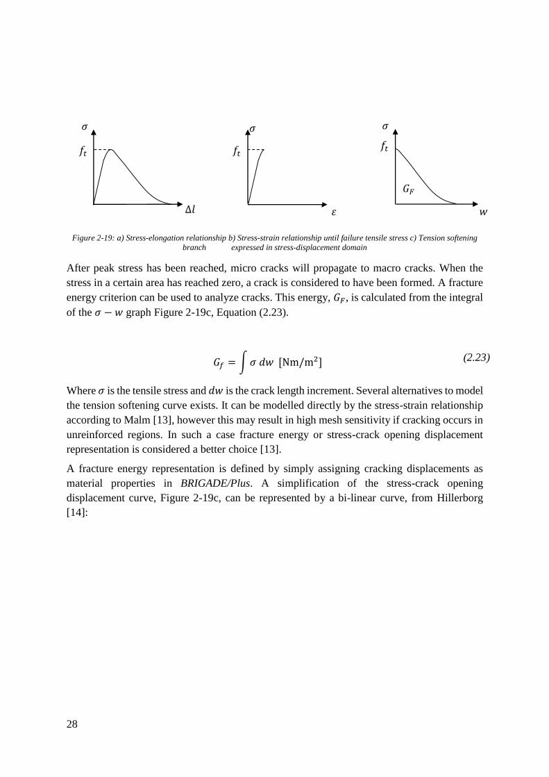
Considering a tensile concrete test, the stress-elongation relationship (similar behavior as
stress-strain relationship) may be seen to the left in Figure 2-19. According to Hillerborg [12],
a suitable way to model cracking of concrete would be to divide the behavior into two parts;
one which represents the behavior until strength of material is reached and one which models
the behavior after strength of material is reached. The latter is often referred to as the ‘tension
softening curve’ [12].
28
Figure 2-19: a) Stress-elongation relationship b) Stress-strain relationship until failure tensile stress c) Tension softening
branch expressed in stress-displacement domain
After peak stress has been reached, micro cracks will propagate to macro cracks. When the
stress in a certain area has reached zero, a crack is considered to have been formed. A fracture
energy criterion can be used to analyze cracks. This energy, 𝐺𝐹, is calculated from the integral
of the 𝜎 − 𝑤 graph Figure 2-19c, Equation (2.23).
𝐺𝑓 = ∫ 𝜎 𝑑𝑤 [Nm/m2] (2.23)
Where 𝜎 is the tensile stress and 𝑑𝑤 is the crack length increment. Several alternatives to model
the tension softening curve exists. It can be modelled directly by the stress-strain relationship
according to Malm [13], however this may result in high mesh sensitivity if cracking occurs in
unreinforced regions. In such a case fracture energy or stress-crack opening displacement
representation is considered a better choice [13].
A fracture energy representation is defined by simply assigning cracking displacements as
material properties in BRIGADE/Plus. A simplification of the stress-crack opening
displacement curve, Figure 2-19c, can be represented by a bi-linear curve, from Hillerborg
[14]:
𝜎
Δ𝑙
𝜎
𝑓𝑡 𝑓𝑡 𝑓𝑡
𝜀
𝜎
𝑤
𝐺𝐹
29
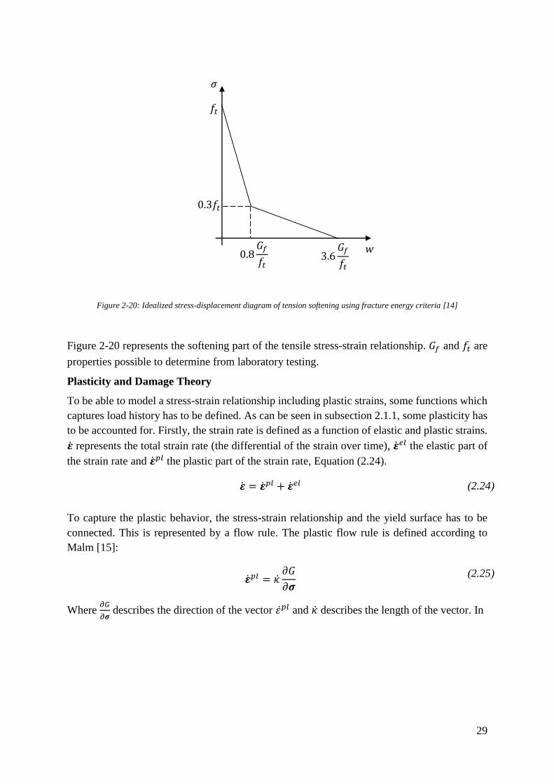
Figure 2-20: Idealized stress-displacement diagram of tension softening using fracture energy criteria [14]
Figure 2-20 represents the softening part of the tensile stress-strain relationship. 𝐺𝑓 and 𝑓𝑡 are
properties possible to determine from laboratory testing.
Plasticity and Damage Theory
To be able to model a stress-strain relationship including plastic strains, some functions which
captures load history has to be defined. As can be seen in subsection 2.1.1, some plasticity has
to be accounted for. Firstly, the strain rate is defined as a function of elastic and plastic strains.
�̇� represents the total strain rate (the differential of the strain over time), �̇�𝑒𝑙 the elastic part of
the strain rate and �̇�𝑝𝑙 the plastic part of the strain rate, Equation (2.24).
�̇� = �̇�𝑝𝑙 + �̇�𝑒𝑙 (2.24)
To capture the plastic behavior, the stress-strain relationship and the yield surface has to be
connected. This is represented by a flow rule. The plastic flow rule is defined according to
Malm [15]:
�̇�𝑝𝑙 = �̇�
𝜕𝐺
𝜕𝝈
(2.25)
Where 𝜕𝐺
𝜕𝝈 describes the direction of the vector 𝜀̇𝑝𝑙 and �̇� describes the length of the vector. In
𝑓𝑡
𝜎
𝑤
0.3𝑓𝑡
0.8𝐺𝑓
𝑓𝑡 3.6
𝐺𝑓
𝑓𝑡
30
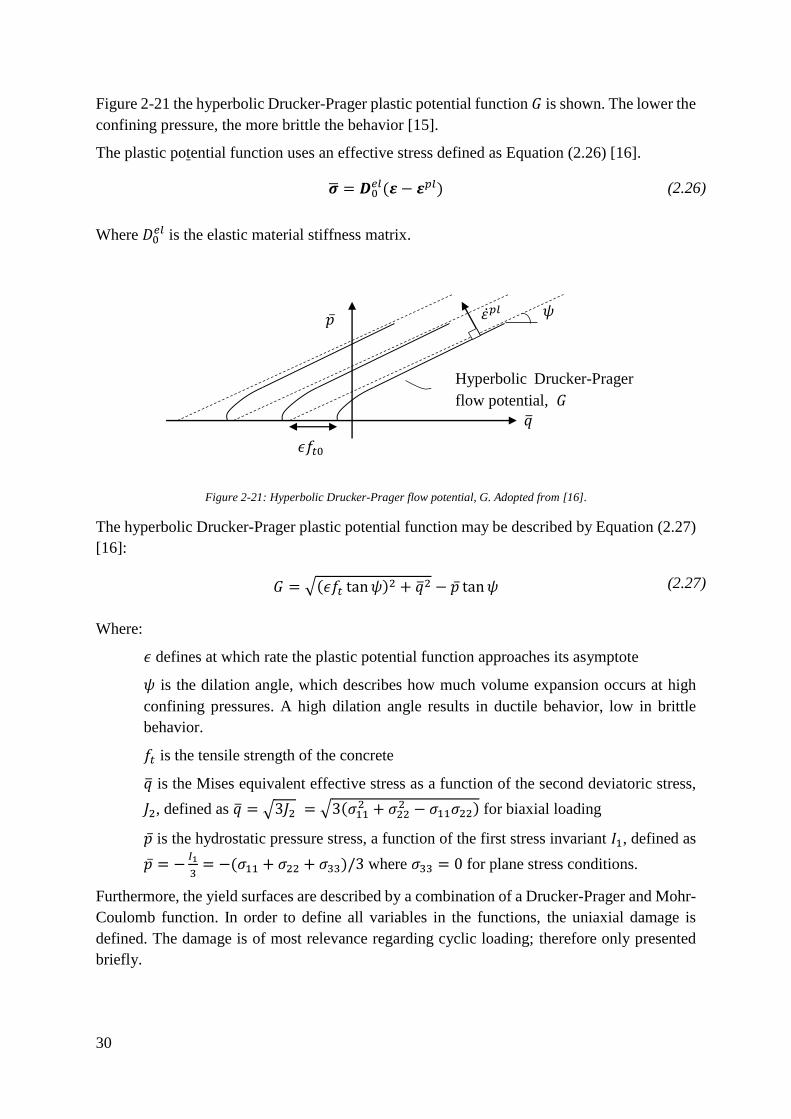
Figure 2-21 the hyperbolic Drucker-Prager plastic potential function 𝐺 is shown. The lower the
confining pressure, the more brittle the behavior [15].
The plastic potential function uses an effective stress defined as Equation (2.26) [16].
�̅� = 𝑫0𝑒𝑙(𝜺 − 𝜺𝑝𝑙) (2.26)
Where 𝐷0𝑒𝑙 is the elastic material stiffness matrix.
Figure 2-21: Hyperbolic Drucker-Prager flow potential, G. Adopted from [16].
The hyperbolic Drucker-Prager plastic potential function may be described by Equation (2.27)
[16]:
𝐺 = √(𝜖𝑓𝑡 tan 𝜓)2 + �̅�2 − �̅� tan 𝜓 (2.27)
Where:
𝜖 defines at which rate the plastic potential function approaches its asymptote
𝜓 is the dilation angle, which describes how much volume expansion occurs at high
confining pressures. A high dilation angle results in ductile behavior, low in brittle
behavior.
𝑓𝑡 is the tensile strength of the concrete
�̅� is the Mises equivalent effective stress as a function of the second deviatoric stress,
𝐽2, defined as �̅� = √3𝐽2 = √3(𝜎112 + 𝜎22
2 − 𝜎11𝜎22) for biaxial loading
�̅� is the hydrostatic pressure stress, a function of the first stress invariant 𝐼1, defined as
�̅� = −𝐼1
3= −(𝜎11 + 𝜎22 + 𝜎33)/3 where 𝜎33 = 0 for plane stress conditions.
Furthermore, the yield surfaces are described by a combination of a Drucker-Prager and Mohr-
Coulomb function. In order to define all variables in the functions, the uniaxial damage is
defined. The damage is of most relevance regarding cyclic loading; therefore only presented
briefly.
𝜀̇𝑝𝑙 𝜓
Hyperbolic Drucker-Prager
flow potential, 𝐺
�̅�
�̅�
𝜖𝑓𝑡0
31
It is not realistic that, if the material is unloaded, the stiffness of the material would remain.
Therefore a damage parameter 𝑑𝑡 and 𝑑𝑐 are defined, which degrade the initial modulus of
elasticity according to Equation (2.28) and (2.29).
𝜎𝑡 = (1 − 𝑑𝑡)𝐸0(𝜀𝑡 − 𝜀�̃�𝑝𝑙) (2.28)
𝜎𝑐 = (1 − 𝑑𝑐)𝐸0(𝜀𝑐 − 𝜀�̃�𝑝𝑙) (2.29)
Where 𝜀�̃�𝑝𝑙
& 𝜀�̃�𝑝𝑙
are the plastic strains which remain if the material is unloaded. As the cracks
yield less load carrying area, an effective stress for uniaxial loading is defined as Equation
(2.30) and (2.31):
𝜎𝑡 = 𝐸0(𝜀𝑡 − 𝜀�̃�𝑝𝑙
) (2.30)
𝜎𝑐 = 𝐸0(𝜀𝑐 − 𝜀�̃�𝑝𝑙) (2.31)
These stresses are called the effective tensile and compressive cohesion stresses respectively.
Since no unloading and reloading of the specimens is of interest, no damage parameters are
specified.
32
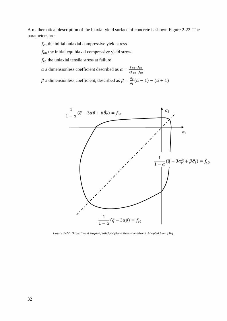
A mathematical description of the biaxial yield surface of concrete is shown Figure 2-22. The
parameters are:
𝑓𝑐0 the initial uniaxial compressive yield stress
𝑓𝑏0 the initial equibiaxal compressive yield stress
𝑓𝑡0 the uniaxial tensile stress at failure
𝛼 a dimensionless coefficient described as 𝛼 =𝑓𝑏0−𝑓𝑐0
2𝑓𝑏0−𝑓𝑐0
𝛽 a dimensionless coefficient, described as 𝛽 =�̅�𝑐
�̅�𝑡(𝛼 − 1) − (𝛼 + 1)
Figure 2-22: Biaxial yield surface, valid for plane stress conditions. Adopted from [16].
1
1 − 𝛼(�̅� − 3𝛼�̅� + 𝛽𝜎2) = 𝑓𝑐0
1
1 − 𝛼(�̅� − 3𝛼�̅� + 𝛽𝜎1) = 𝑓𝑐0
1
1 − 𝛼(�̅� − 3𝛼�̅�) = 𝑓𝑐0
𝜎2
𝜎1
33
Furthermore, a so-called yield function needs to be defined. In BRIGADE/Plus, this is defined
as Equation (2.32).
𝐹 =
1
1 − 𝛼(𝑞 − 3𝛼𝑝 + 𝛽(�̃�𝑝𝑙)⟨�̅�max⟩ − 𝛾⟨𝜎max⟩) − 𝜎𝑐(𝜀�̃�
𝑝𝑙) ≤ 0 (2.32)
Where all parameters except 𝛾 are described above. 𝛾 is defined as Equation (2.33).
𝛾 =3(1 − 𝐾𝑐)
2 𝐾𝑐 − 1
(2.33)
𝐾𝑐, which describes the relationship between the tensile meridian 𝑞𝑇𝑀 and the compressive
meridian 𝑞𝐶𝑀, according to Equation (2.34) [17] [18].
𝐾𝑐 =(√𝐽2)
𝑇𝑀
(√𝐽2)𝐶𝑀
(2.34)
Where 𝐽2 is the second invariant of the stress deviator [18].
In order to reach convergence when the concrete starts to crack, a so-called viscoplastic
regularization is introduced. The viscoplastic strain tensor is defined as Equation (2.35). [16]
�̇�𝑣𝑝𝑙 =
1
𝜇(𝜺𝑝𝑙 − 𝜺𝑣
𝑝𝑙) (2.35)
Where the viscosity parameter 𝜇 represents the relaxation time of the viscoplastic system and
𝜺𝑝𝑙 is the plastic strain as defined above.
The viscoplastic stress-strain model is defined according to Equation (2.36).
𝜎 = (1 − 𝑑𝑣)𝐷0(𝜀 − 𝜀𝑣𝑝𝑙) (2.36)
The viscoplastic system converge towards the original system when Δ𝑡
𝜇→ ∞, where Δ𝑡 is the
characteristic time increment.

34
35
3 CALCULATION PROCEDURE
The following chapter shows how to design a specimen according to the strut-and-tie method.
The calculations regarding the specimens are presented in Appendix B. These results are based
on three different angles, where 𝛼 = 60° complies with current standards and practices.
The desired type of failure in beams T1-T4 are so called flexure failures, i.e. the beam bends
which leads to tensile strain in the primary reinforcement in the bottom and ultimately yielding
and failure. In addition to the control of each strut and tie in the truss model the nodes, where
these struts and ties meet, are checked. Some of these nodes are subjected purely to
compression whereas some are subjected to compression and tension simultaneously. Section
3.1 - 3.3 are intended to give the reader basic knowledge in the design process using the strut-
and-tie method, whilst section 3.4 presents calculations needed to determine the load-bearing
capacity of the specimens.
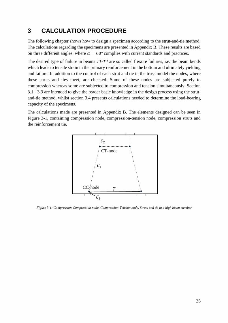
The calculations made are presented in Appendix B. The elements designed can be seen in
Figure 3-1, containing compression node, compression-tension node, compression struts and
the reinforcement tie.
Figure 3-1: Compression-Compression node, Compression-Tension node, Struts and tie in a high beam member
𝐶2
𝐶1
𝐶2
𝑇 CC-node
CT-node
36
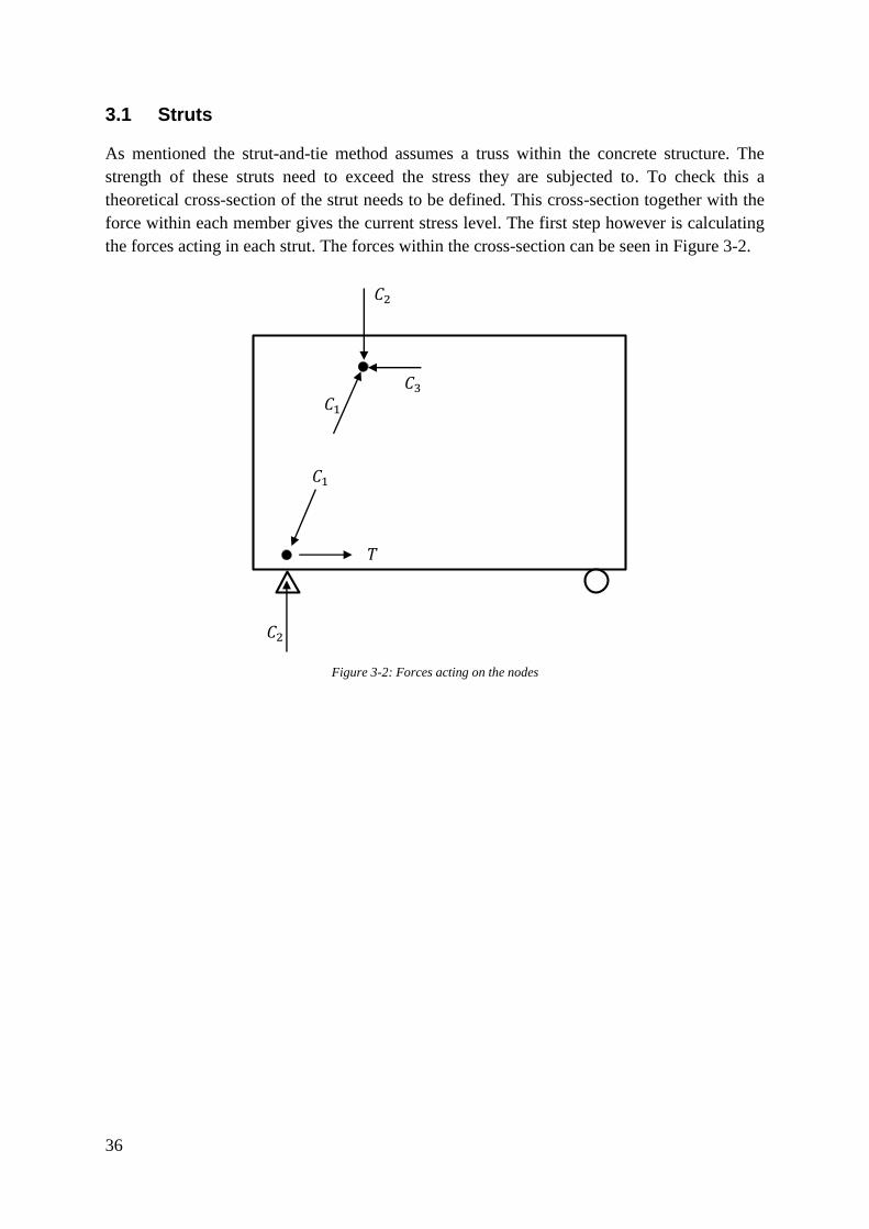
3.1 Struts
As mentioned the strut-and-tie method assumes a truss within the concrete structure. The
strength of these struts need to exceed the stress they are subjected to. To check this a
theoretical cross-section of the strut needs to be defined. This cross-section together with the
force within each member gives the current stress level. The first step however is calculating
the forces acting in each strut. The forces within the cross-section can be seen in Figure 3-2.
Figure 3-2: Forces acting on the nodes
𝐶1
𝐶1
𝐶2
𝐶2
𝐶3
𝑇
37
3.1.1 Forces
As the forces at each node needs to be in equilibrium, each of the internal strut forces can be
calculated with calculations shown below, Equations (3.1)-(3.3). The forces depends solely
on the externally applied force, F, and the internal angle, 𝛼.
𝐶1 =
𝐹/2
sin 𝛼
(3.1)
𝐶2 = 𝐹/2 (3.2)
𝐶3 =
𝐹/2
tan 𝛼
(3.3)
The fictive area for these struts depend primary on the area of the steel plates where the external
loads are applied, as well as the steel supports.
3.1.2 Capacities
The strut strengths are normally of no concern, however, if no secondary reinforcement is
provided and cracks transverse to the force direction develops this could be an issue [8]. In
such a case the strut strength is calculated as Equation (3.4):
𝜎𝑅𝑑,𝑚𝑎𝑥 = 0,6 ∙ 𝜈′ ∙ 𝑓𝑐𝑑 (3.4)
Where 𝜈′ is presented later in Equation (3.6), and 𝑓𝑐𝑑 is used since failure in the struts are
undesirable.
38
3.2 Nodes
The strength of the nodes varies depending on the type of load they are subjected to, see
subsection 2.1.1. A node only subjected to compressive stresses is assumed to have a higher
strength than a node subjected to tensile and compressive stresses simultaneously. The
capacities should be compared to the strut forces, presented in subsection 3.1.1, acting on the
faces of the nodes.
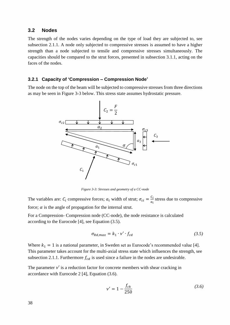
3.2.1 Capacity of ‘Compression – Compression Node’
The node on the top of the beam will be subjected to compressive stresses from three directions
as may be seen in Figure 3-3 below. This stress state assumes hydrostatic pressure.
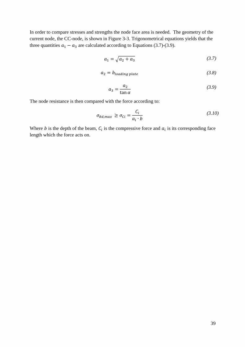
Figure 3-3: Stresses and geometry of a CC-node
The variables are: 𝐶𝑖 compressive forces; 𝑎𝑖 width of strut; 𝜎𝑐𝑖 =𝐶𝑖
𝑎𝑖 stress due to compressive
force; 𝛼 is the angle of propagation for the internal strut.
For a Compression- Compression node (CC-node), the node resistance is calculated
according to the Eurocode [4], see Equation (3.5).
𝜎𝑅𝑑,𝑚𝑎𝑥 = 𝑘1 ∙ 𝜈′ ∙ 𝑓𝑐𝑑 (3.5)
Where 𝑘1 = 1 is a national parameter, in Sweden set as Eurocode’s recommended value [4].
This parameter takes account for the multi-axial stress state which influences the strength, see
subsection 2.1.1. Furthermore 𝑓𝑐𝑑 is used since a failure in the nodes are undesirable.
The parameter 𝜈′ is a reduction factor for concrete members with shear cracking in
accordance with Eurocode 2 [4], Equation (3.6).
𝜈′ = 1 −
𝑓𝑐𝑘
250
(3.6)
𝐶2 =𝐹
2
𝛼
𝑎2
𝑎3
𝜎𝑐3
𝜎𝑐2
𝜎𝑐1
𝑎1
𝐶1
𝐶3
39
In order to compare stresses and strengths the node face area is needed. The geometry of the
current node, the CC-node, is shown in Figure 3-3. Trigonometrical equations yields that the
three quantities 𝑎1 − 𝑎3 are calculated according to Equations (3.7)-(3.9).
𝑎1 = √𝑎2 + 𝑎3 (3.7)
𝑎2 = 𝑏𝑙𝑜𝑎𝑑𝑖𝑛𝑔 𝑝𝑙𝑎𝑡𝑒 (3.8)
𝑎3 =𝑎2
tan 𝛼 (3.9)
The node resistance is then compared with the force according to:
𝜎𝑅𝑑,𝑚𝑎𝑥 ≥ 𝜎𝐶𝑖 =
𝐶𝑖
𝑎𝑖 ∙ 𝑏 (3.10)
Where 𝑏 is the depth of the beam, 𝐶𝑖 is the compressive force and 𝑎𝑖 is its corresponding face
length which the force acts on.
40
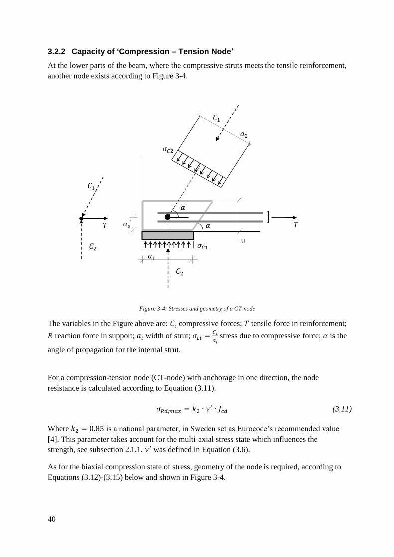
3.2.2 Capacity of ‘Compression – Tension Node’
At the lower parts of the beam, where the compressive struts meets the tensile reinforcement,
another node exists according to Figure 3-4.
Figure 3-4: Stresses and geometry of a CT-node
The variables in the Figure above are: 𝐶𝑖 compressive forces; 𝑇 tensile force in reinforcement;
𝑅 reaction force in support; 𝑎𝑖 width of strut; 𝜎𝑐𝑖 =𝐶𝑖
𝑎𝑖 stress due to compressive force; 𝛼 is the
angle of propagation for the internal strut.
For a compression-tension node (CT-node) with anchorage in one direction, the node
resistance is calculated according to Equation (3.11).
𝜎𝑅𝑑,𝑚𝑎𝑥 = 𝑘2 ∙ 𝜈′ ∙ 𝑓𝑐𝑑 (3.11)
Where 𝑘2 = 0.85 is a national parameter, in Sweden set as Eurocode’s recommended value
[4]. This parameter takes account for the multi-axial stress state which influences the
strength, see subsection 2.1.1. 𝜈′ was defined in Equation (3.6).
As for the biaxial compression state of stress, geometry of the node is required, according to
Equations (3.12)-(3.15) below and shown in Figure 3-4.
𝑇
𝐶1
𝑇
𝐶1
𝑎2
u 𝐶2
𝐶2
𝑎𝑠
𝜎𝐶2
𝜎𝐶1
𝛼
𝑎1
𝛼
41
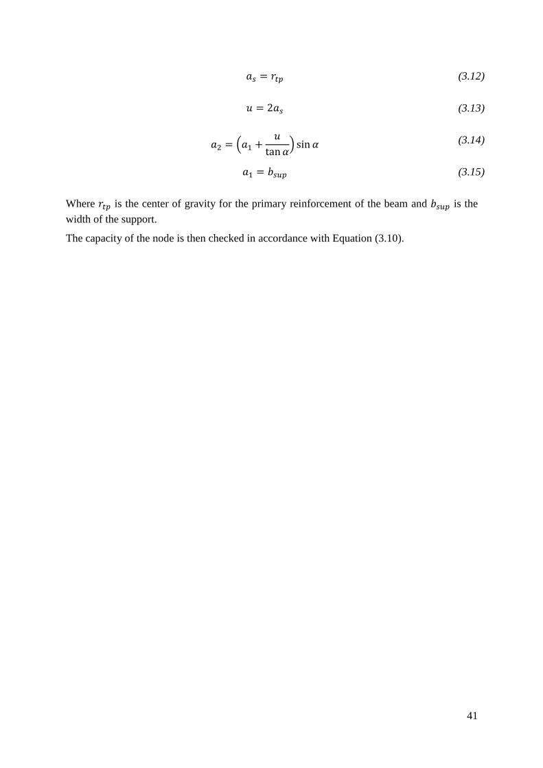
𝑎𝑠 = 𝑟𝑡𝑝 (3.12)
𝑢 = 2𝑎𝑠 (3.13)
𝑎2 = (𝑎1 +𝑢
tan 𝛼) sin 𝛼 (3.14)
𝑎1 = 𝑏𝑠𝑢𝑝 (3.15)
Where 𝑟𝑡𝑝 is the center of gravity for the primary reinforcement of the beam and 𝑏𝑠𝑢𝑝 is the
width of the support.
The capacity of the node is then checked in accordance with Equation (3.10).
42
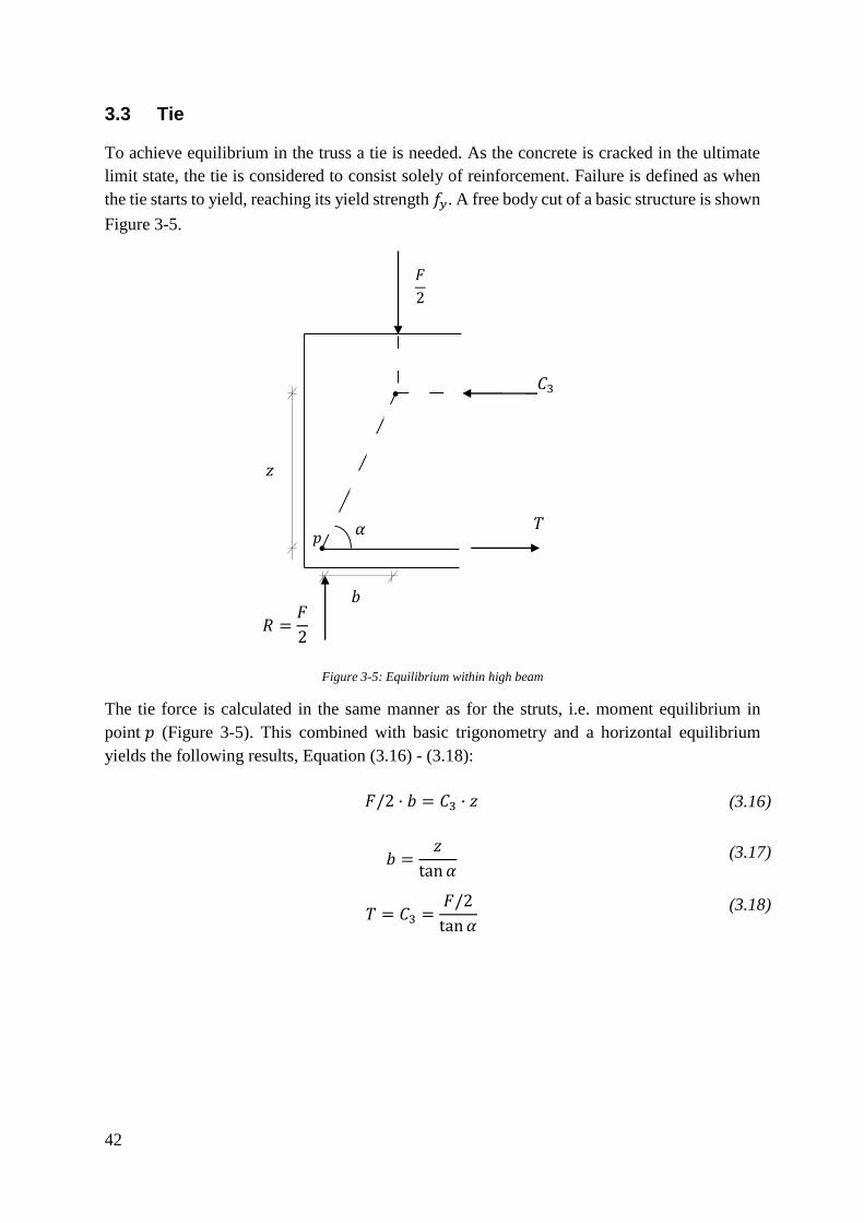
3.3 Tie
To achieve equilibrium in the truss a tie is needed. As the concrete is cracked in the ultimate
limit state, the tie is considered to consist solely of reinforcement. Failure is defined as when
the tie starts to yield, reaching its yield strength 𝑓𝑦. A free body cut of a basic structure is shown
Figure 3-5.
Figure 3-5: Equilibrium within high beam
The tie force is calculated in the same manner as for the struts, i.e. moment equilibrium in
point 𝑝 (Figure 3-5). This combined with basic trigonometry and a horizontal equilibrium
yields the following results, Equation (3.16) - (3.18):
𝐹/2 · 𝑏 = 𝐶3 · 𝑧 (3.16)
𝑏 =𝑧
tan 𝛼 (3.17)
𝑇 = 𝐶3 =
𝐹/2
tan 𝛼
(3.18)
𝐶3
𝑇
𝐹
2
𝑝
𝑏
𝑅 =𝐹
2
𝑧
𝛼
43
The amount of reinforcement is calculated as stated in Equation (3.17).
𝐴𝑠 ≥
𝑇
𝑓𝑦 (3.19)
Where 𝑇 is the tie force and 𝑓𝑦 the yield strength of the reinforcement bars. Choosing a
dimension 𝜙 of the reinforcement gives the required number of bars needed to take the tensile
force 𝑇 where 𝑛𝑟𝑒𝑏𝑎𝑟 is the required number of reinforcement bars according to Equation
(3.20).
𝑛𝑟𝑒𝑏𝑎𝑟 = 𝑟𝑜𝑢𝑛𝑑𝑢𝑝 (𝐴𝑠
𝐴𝑟𝑒𝑏𝑎𝑟) (3.20)
3.4 Load bearing capacity of specimen
Assuming that anchorage failures, node failures and strut failures are prevented (see Appendix
B), capacity of the beam is theoretically decided from three main variables: the internal lever
arm, which is solely decided from the angle 𝛼 in Figure 3-5 and the capacity of the tie, which
depends on amount of reinforcement and its yield strength.
Combining Equation (3.18) and (3.19), the capacity may be calculated as:
𝐹 = 2 ∙ 𝑇 ∙ tan 𝛼 = 2 ∙ 𝑓𝑦 ∙ 𝐴𝑠 ∙ tan 𝛼 (3.21)
3.5 Anchorage length
In the design of a concrete member, anchorage lengths of the reinforcement bars have to be
checked in order to ensure that sufficient anchorage is reached. The specimens have been
designed to prevent anchorage failure in accordance with Eurocode 2 [4]. Practically, the best
way to prevent anchorage failure resulted in extending the specimens lengths outside the
support regions and bending the bars. The reader is referred to Appendix A for drawings and
Appendix B4 for calculations.

44
45
4 LABORATORY PROCESS
In order to determine the reliability and limitations of the strut-and-tie method, verify internal
angles and have results to compare with the numeric model, laboratory tests were carried out.
As many parameters as possible within the time-scope of the project were tested, including
compressive and tensile strength of concrete, fracture energy of the concrete and stress-strain
behavior of the reinforcing steel.
The four beam specimens tested were manufactured at the location where they were to be tested
to be able to supervise the entire process. The concrete was ordered from an external distributer
to assure a good quality concrete with proper features in terms of strength, ratio of aggregates,
adequate distribution of the aggregates throughout the mixture and ratio of water. The concrete
used was of quality C30, with a maximum aggregate size of 16 mm.
The reinforcement steel was ordered and the individual bars were tested according to
subsection 4.1.2.
4.1 Material properties
To make proper estimations of the internal angle in the laboratory test, several material
properties of the included members must be determined. Retrieving these properties makes it
possible to adapt the manual calculations as well as the simulations made in BRIGADE/Plus
to the conditions present at the time of the laboratory practical to get as comparable results as
possible.
4.1.1 Concrete
Three different tests of the concrete were performed in order to determine the properties of the
batch of C30 concrete delivered. One in order to determine the compressive strength, one in
order to determine the tensile strength and one in order to determine the fracture energy.
Compressive strength test
When ordered, a hint about the strength of the concrete was given. However, in order to get a
more precise perception of the material parameters the delivered batch of concrete was tested.
This was tested by subjecting a cube with a side length of 150 mm to compression, which have
been left to cure for 28 days in 100% relative humidity.
From the applied force F needed to crush the specimen the strength of the concrete can be
derived, see Equation (4.1).
𝑓𝑐𝑐 =
𝐹
𝐴
(4.1)
46
Tensile strength test – Brazilian test
The ideal case would be to subject the specimen to a pure tensile force but since anchoring of
the specimen would prove a problem another solution is used. A spitting test, also known as a
Brazilian test, was performed. This was done by subjecting a cylindrical specimen, diameter of
150 mm and height of 300 mm, to a distributed load along top and bottom perimeter [19]. The
force applied generated a tension force perpendicular to the load direction due to the Poisson’s
effect, and eventually cause the cylinder to split down the middle. Knowing the force needed
to split the specimen the concrete splitting tensile strength 𝑓𝑐𝑡,𝑠𝑝 can be derived, Equation (4.2).
𝑓𝑐𝑡,𝑠𝑝 =
2𝑃
𝜋𝐷𝐿
(4.2)
Figure 4-1: Brazilian test setup
The relation between the calculated splitting tensile strength and the approximate tensile
strength of the material is decided according to Equation (4.3) [20].
𝑓𝑐𝑡 = 0.9 · 𝑓𝑐𝑡,𝑠𝑝 (4.3)
Fracture energy test
In order to model the concrete in BRIGADE/Plus, a fracture energy approach is used, see
subsection 0. Concrete cracking behavior is difficult to model and literature may be
contradictory regarding choice of parameters. Therefore, the authors have chosen to perform a
fracture energy test.
The theoretical basis of the concrete cracking behavior is described in subsection 0. According
to Hillerborg [12], the best method would be to test the uniaxial tensile strength in order to get
the full stress-strain response curve of the material. However, as mentioned, these tests are
difficult to perform and require advanced equipment. An alternative method proposed by
Hillerborg [12] suggests that the fracture energy may be defined from a three-point bending
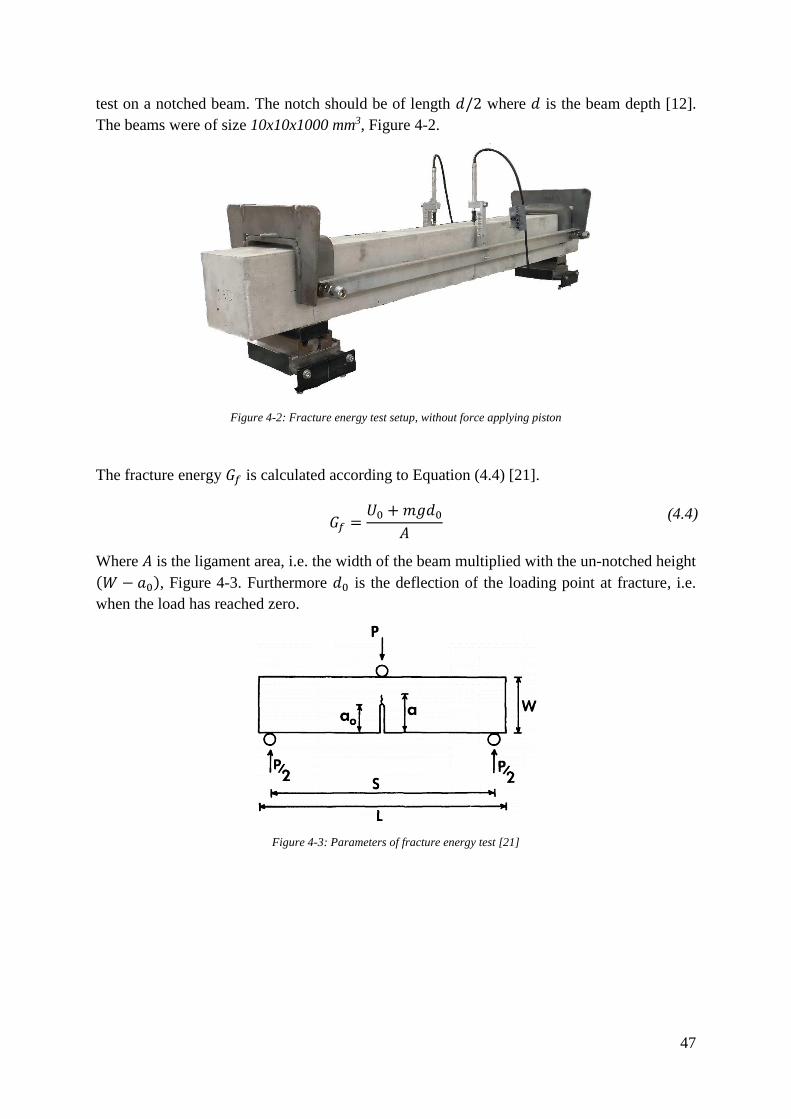
47
test on a notched beam. The notch should be of length 𝑑/2 where 𝑑 is the beam depth [12].
The beams were of size 10x10x1000 mm3, Figure 4-2.
Figure 4-2: Fracture energy test setup, without force applying piston
The fracture energy 𝐺𝑓 is calculated according to Equation (4.4) [21].
𝐺𝑓 =
𝑈0 + 𝑚𝑔𝑑0
𝐴
(4.4)
Where 𝐴 is the ligament area, i.e. the width of the beam multiplied with the un-notched height
(𝑊 − 𝑎0), Figure 4-3. Furthermore 𝑑0 is the deflection of the loading point at fracture, i.e.
when the load has reached zero.
Figure 4-3: Parameters of fracture energy test [21]
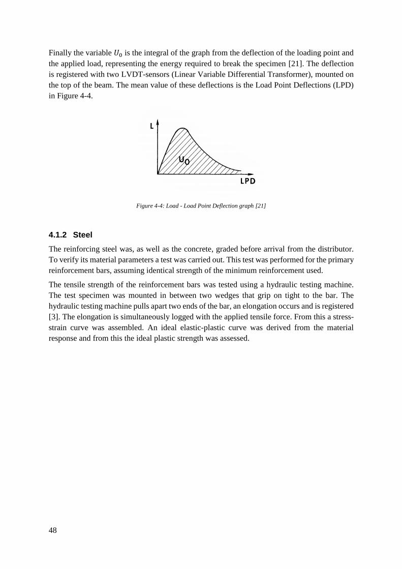
48
Finally the variable 𝑈0 is the integral of the graph from the deflection of the loading point and
the applied load, representing the energy required to break the specimen [21]. The deflection
is registered with two LVDT-sensors (Linear Variable Differential Transformer), mounted on
the top of the beam. The mean value of these deflections is the Load Point Deflections (LPD)
in Figure 4-4.
Figure 4-4: Load - Load Point Deflection graph [21]
4.1.2 Steel
The reinforcing steel was, as well as the concrete, graded before arrival from the distributor.
To verify its material parameters a test was carried out. This test was performed for the primary
reinforcement bars, assuming identical strength of the minimum reinforcement used.
The tensile strength of the reinforcement bars was tested using a hydraulic testing machine.
The test specimen was mounted in between two wedges that grip on tight to the bar. The
hydraulic testing machine pulls apart two ends of the bar, an elongation occurs and is registered
[3]. The elongation is simultaneously logged with the applied tensile force. From this a stress-
strain curve was assembled. An ideal elastic-plastic curve was derived from the material
response and from this the ideal plastic strength was assessed.
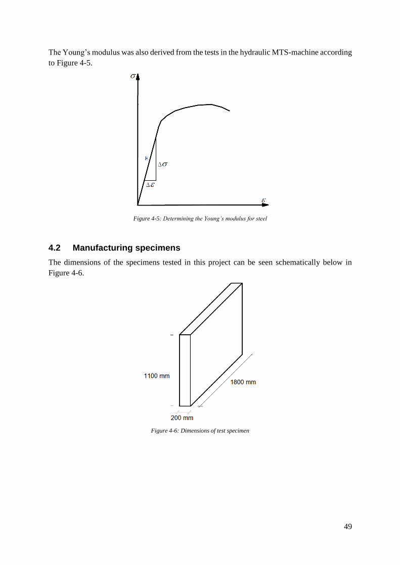
49
The Young’s modulus was also derived from the tests in the hydraulic MTS-machine according
to Figure 4-5.
Figure 4-5: Determining the Young’s modulus for steel
4.2 Manufacturing specimens
The dimensions of the specimens tested in this project can be seen schematically below in
Figure 4-6.
Figure 4-6: Dimensions of test specimen
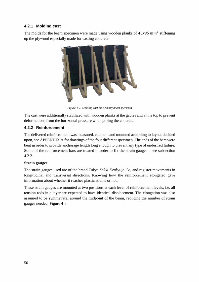
50
4.2.1 Molding cast
The molds for the beam specimen were made using wooden planks of 45𝑥95 𝑚𝑚2 stiffening
up the plywood especially made for casting concrete.
Figure 4-7: Molding cast for primary beam specimen
The cast were additionally stabilized with wooden planks at the gables and at the top to prevent
deformations from the horizontal pressure when poring the concrete.
4.2.2 Reinforcement
The delivered reinforcement was measured, cut, bent and mounted according to layout decided
upon, see APPENDIX A for drawings of the four different specimen. The ends of the bars were
bent in order to provide anchorage length long enough to prevent any type of undesired failure.
Some of the reinforcement bars are treated in order to fix the strain gauges – see subsection
4.2.2.
Strain gauges
The strain gauges used are of the brand Tokyo Sokki Kenkyujo Co, and register movements in
longitudinal and transversal directions. Knowing how the reinforcement elongated gave
information about whether it reaches plastic strains or not.
These strain gauges are mounted at two positions at each level of reinforcement levels, i.e. all
tension rods in a layer are expected to have identical displacement. The elongation was also
assumed to be symmetrical around the midpoint of the beam, reducing the number of strain
gauges needed, Figure 4-8.
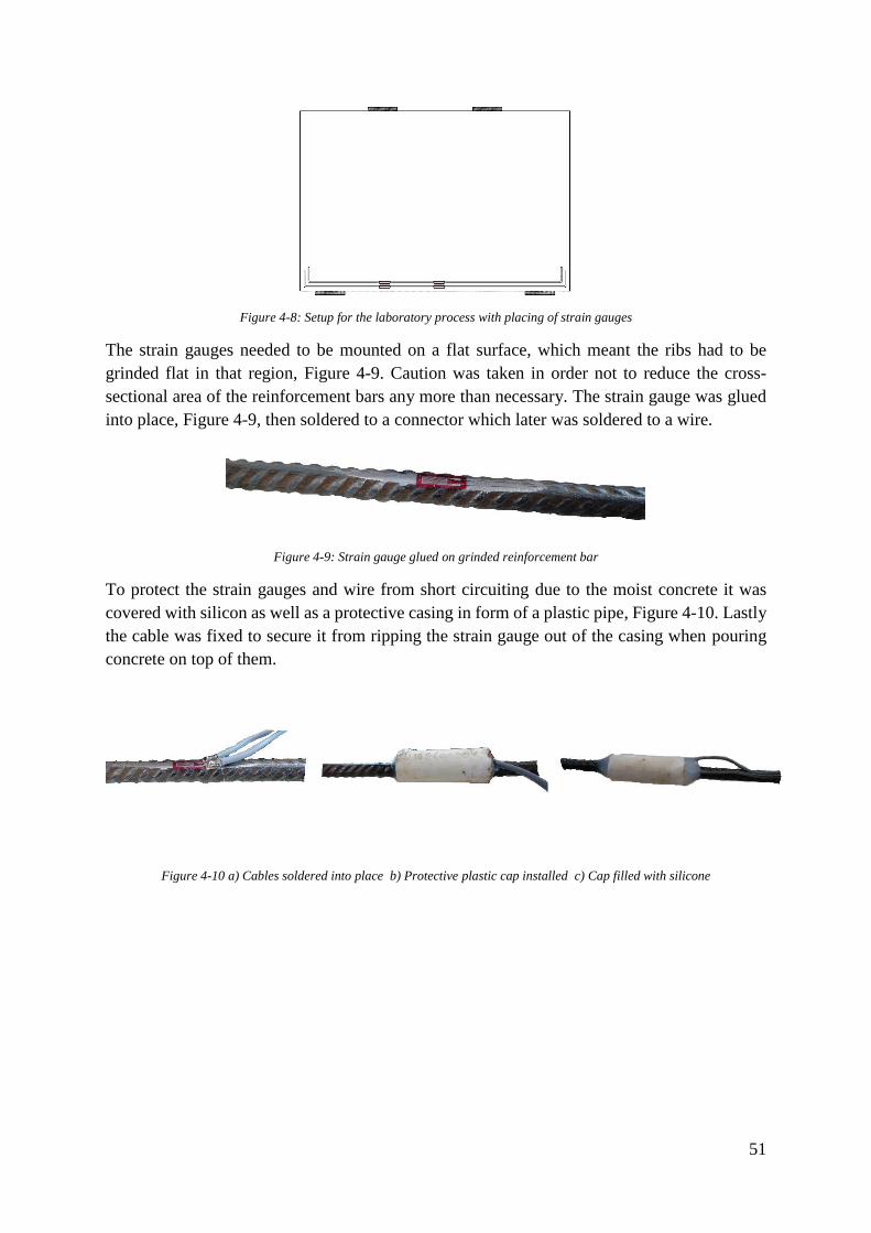
51
Figure 4-8: Setup for the laboratory process with placing of strain gauges
The strain gauges needed to be mounted on a flat surface, which meant the ribs had to be
grinded flat in that region, Figure 4-9. Caution was taken in order not to reduce the cross-
sectional area of the reinforcement bars any more than necessary. The strain gauge was glued
into place, Figure 4-9, then soldered to a connector which later was soldered to a wire.
Figure 4-9: Strain gauge glued on grinded reinforcement bar
To protect the strain gauges and wire from short circuiting due to the moist concrete it was
covered with silicon as well as a protective casing in form of a plastic pipe, Figure 4-10. Lastly
the cable was fixed to secure it from ripping the strain gauge out of the casing when pouring
concrete on top of them.
Figure 4-10 a) Cables soldered into place b) Protective plastic cap installed c) Cap filled with silicone
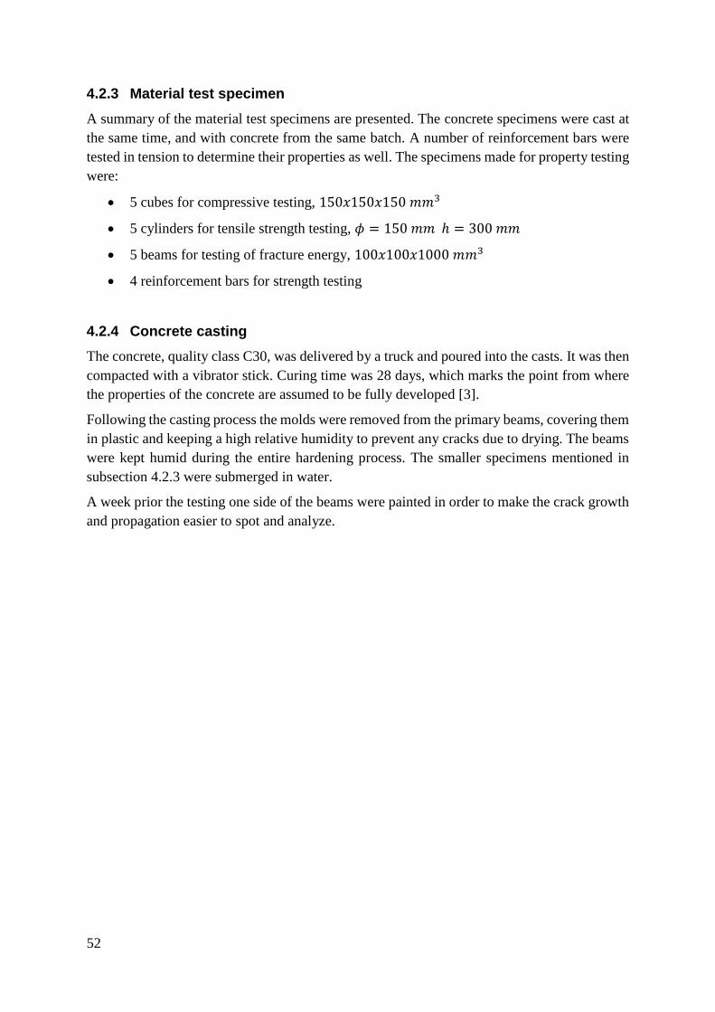
52
4.2.3 Material test specimen
A summary of the material test specimens are presented. The concrete specimens were cast at
the same time, and with concrete from the same batch. A number of reinforcement bars were
tested in tension to determine their properties as well. The specimens made for property testing
were:
5 cubes for compressive testing, 150𝑥150𝑥150 𝑚𝑚3
5 cylinders for tensile strength testing, 𝜙 = 150 𝑚𝑚 ℎ = 300 𝑚𝑚
5 beams for testing of fracture energy, 100𝑥100𝑥1000 𝑚𝑚3
4 reinforcement bars for strength testing
4.2.4 Concrete casting
The concrete, quality class C30, was delivered by a truck and poured into the casts. It was then
compacted with a vibrator stick. Curing time was 28 days, which marks the point from where
the properties of the concrete are assumed to be fully developed [3].
Following the casting process the molds were removed from the primary beams, covering them
in plastic and keeping a high relative humidity to prevent any cracks due to drying. The beams
were kept humid during the entire hardening process. The smaller specimens mentioned in
subsection 4.2.3 were submerged in water.
A week prior the testing one side of the beams were painted in order to make the crack growth
and propagation easier to spot and analyze.
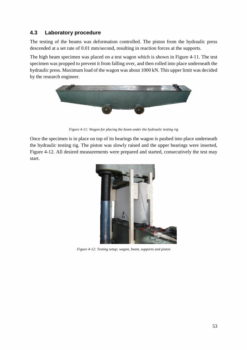
53
4.3 Laboratory procedure
The testing of the beams was deformation controlled. The piston from the hydraulic press
descended at a set rate of 0.01 mm/second, resulting in reaction forces at the supports.
The high beam specimen was placed on a test wagon which is shown in Figure 4-11. The test
specimen was propped to prevent it from falling over, and then rolled into place underneath the
hydraulic press. Maximum load of the wagon was about 1000 kN. This upper limit was decided
by the research engineer.
Figure 4-11: Wagon for placing the beam under the hydraulic testing rig
Once the specimen is in place on top of its bearings the wagon is pushed into place underneath
the hydraulic testing rig. The piston was slowly raised and the upper bearings were inserted,
Figure 4-12. All desired measurements were prepared and started, consecutively the test may
start.
Figure 4-12: Testing setup; wagon, beam, supports and piston
54
4.4 Measurements
Several measurements and documentations were made. Some of the data achieved was used in
this project but is available for future research. What was measured and documented were:
Applied force
Strain on the reinforcement, measured with strain gauges
Deflection of beam, measured with deflection gauge
Deflection of table where the beam is mounted
Movement of the piston
Crack propagation and size, photographed next to ruler to later determine crack growth
on the painted face of the beam
Filming as documentation as well as for use in education
55
5 COMPUTER MODELLING
This chapter is intended to give the reader an overview of the computer model used. From this
description the interested reader should be able to reproduce the simulations.
5.1 Model
The following subsections present information needed to re-create this simulation, such as the
material parameters and assumptions made.
5.1.1 Parts
A model consisting of two different parts were created; the high concrete beam member and
the reinforcement bars. Naturally, these will have different material properties. The geometries
of the models were the same as tested in the lab.
The beam was modelled as a 2D-planar shell element and given the depth of 0.2 m. The
reinforcement bars were modelled as 2D-planar wire elements with a given cross-sectional
area.
5.1.2 Material properties
Cracking of concrete affects the strength of the beam, therefore an effort to model this behavior
has to be made. Several cracking models are available in the software. The one used for this
project is the Concrete Damaged Plasticity model, CDP [22]. Basic material properties are
presented in Table 5-1.
Table 5-1: Concrete properties, Density and Elasticity
Density, 𝜌 2400 𝑘𝑔/𝑚3
Young’s modulus, 𝐸 33 𝐺𝑃𝑎
Poisson’s ratio, 𝜈 0.2
The primary parameters in the CDP-modelling follows the recommendations in the Abaqus
Manual [17], Table 5-2, and their features are explained in subsection 0. The dilation angle is
chosen in conformation with literature, e.g. [13].
Table 5-2: Concrete properties, CDP Plasticity
Dilation angle
(𝜓)
Eccentricity (𝜖) 𝑓𝑏0/𝑓𝑐0 𝐾𝑐 Viscosity
Parameter 𝜇
37° 0.1 1.16 0.667 1·10-6
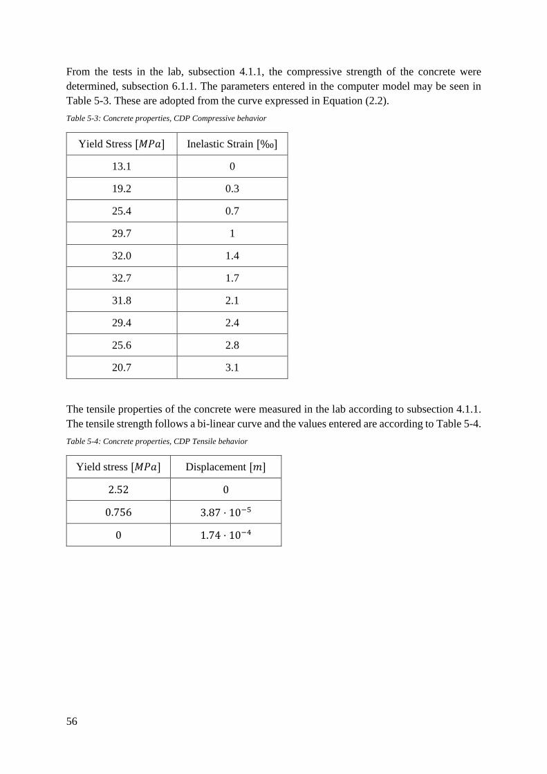
56
From the tests in the lab, subsection 4.1.1, the compressive strength of the concrete were
determined, subsection 6.1.1. The parameters entered in the computer model may be seen in
Table 5-3. These are adopted from the curve expressed in Equation (2.2).
Table 5-3: Concrete properties, CDP Compressive behavior
Yield Stress [𝑀𝑃𝑎] Inelastic Strain [‰]
13.1 0
19.2 0.3
25.4 0.7
29.7 1
32.0 1.4
32.7 1.7
31.8 2.1
29.4 2.4
25.6 2.8
20.7 3.1
The tensile properties of the concrete were measured in the lab according to subsection 4.1.1.
The tensile strength follows a bi-linear curve and the values entered are according to Table 5-4.
Table 5-4: Concrete properties, CDP Tensile behavior
Yield stress [𝑀𝑃𝑎] Displacement [𝑚]
2.52 0
0.756 3.87 · 10−5
0 1.74 · 10−4
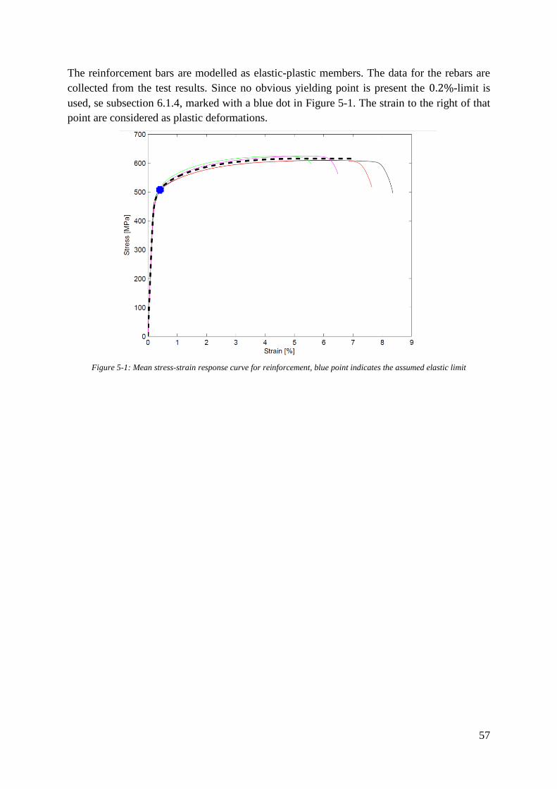
57
The reinforcement bars are modelled as elastic-plastic members. The data for the rebars are
collected from the test results. Since no obvious yielding point is present the 0.2%-limit is
used, se subsection 6.1.4, marked with a blue dot in Figure 5-1. The strain to the right of that
point are considered as plastic deformations.
Figure 5-1: Mean stress-strain response curve for reinforcement, blue point indicates the assumed elastic limit
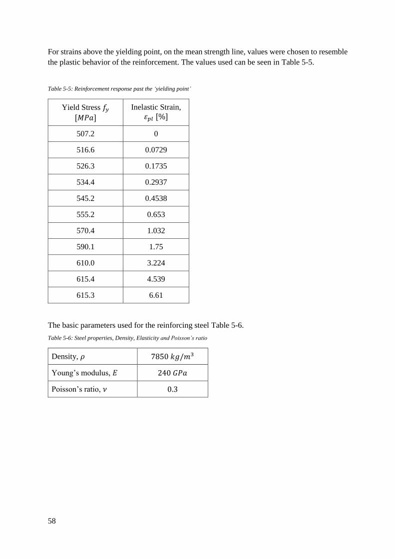
58
For strains above the yielding point, on the mean strength line, values were chosen to resemble
the plastic behavior of the reinforcement. The values used can be seen in Table 5-5.
Table 5-5: Reinforcement response past the ‘yielding point’
Yield Stress 𝑓𝑦
[𝑀𝑃𝑎]
Inelastic Strain,
𝜀𝑝𝑙 [%]
507.2 0
516.6 0.0729
526.3 0.1735
534.4 0.2937
545.2 0.4538
555.2 0.653
570.4 1.032
590.1 1.75
610.0 3.224
615.4 4.539
615.3 6.61
The basic parameters used for the reinforcing steel Table 5-6.
Table 5-6: Steel properties, Density, Elasticity and Poisson’s ratio
Density, 𝜌 7850 𝑘𝑔/𝑚3
Young’s modulus, 𝐸 240 𝐺𝑃𝑎
Poisson’s ratio, 𝜈 0.3
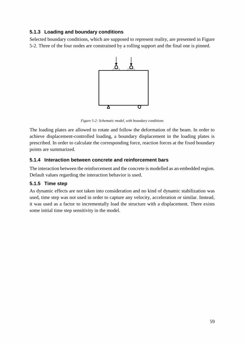
59
5.1.3 Loading and boundary conditions
Selected boundary conditions, which are supposed to represent reality, are presented in Figure
5-2. Three of the four nodes are constrained by a rolling support and the final one is pinned.
Figure 5-2: Schematic model, with boundary conditions
The loading plates are allowed to rotate and follow the deformation of the beam. In order to
achieve displacement-controlled loading, a boundary displacement in the loading plates is
prescribed. In order to calculate the corresponding force, reaction forces at the fixed boundary
points are summarized.
5.1.4 Interaction between concrete and reinforcement bars
The interaction between the reinforcement and the concrete is modelled as an embedded region.
Default values regarding the interaction behavior is used.
5.1.5 Time step
As dynamic effects are not taken into consideration and no kind of dynamic stabilization was
used, time step was not used in order to capture any velocity, acceleration or similar. Instead,
it was used as a factor to incrementally load the structure with a displacement. There exists
some initial time step sensitivity in the model.
60
The time steps used are according to Table 5-7.
Table 5-7: Time step parameters used
Initial time step 1·10-4
Minimum time step 1·10-6
Maximum time step 1·10-4
Data is extracted every time unit of 1·10-4 seconds in order to limit the amount of extracted
data, generating faster data processing times. Thus, the maximum time step is 1·10-4 seconds.
5.1.6 Mesh
In order to model stresses and force response accurately, a quite coarse mesh might be used
according to Malm [15]. However, in order to model cracking behavior in an accurate way,
finer mesh is preferable. In these studies, a coarse mesh has proven to capture the load-
displacement behavior accurately.
Furthermore, shear locking is a phenomena associated with node types and is a risk when using
isoparametric linear 4-node elements that might increase the stiffness of the model
significantly. In order to avoid such response ‘reduced integration’ can be used. Also, the linear
4-node elements have proven insufficient when the deformations are simulated. Therefore
quadratic 8-node elements were used.
The mesh size finally used in the models are of the size 0.1𝑥0.1 𝑚2. This proved to yield good
results in terms of forces.
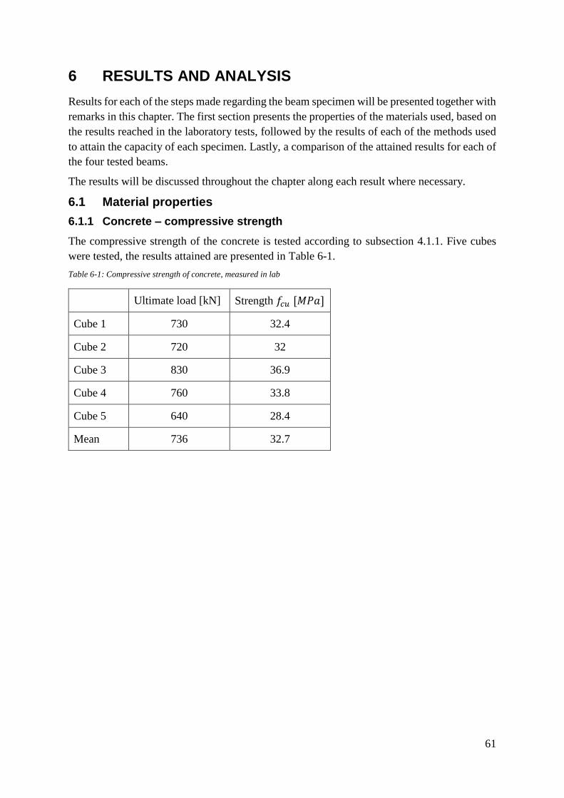
61
6 RESULTS AND ANALYSIS
Results for each of the steps made regarding the beam specimen will be presented together with
remarks in this chapter. The first section presents the properties of the materials used, based on
the results reached in the laboratory tests, followed by the results of each of the methods used
to attain the capacity of each specimen. Lastly, a comparison of the attained results for each of
the four tested beams.
The results will be discussed throughout the chapter along each result where necessary.
6.1 Material properties
6.1.1 Concrete – compressive strength
The compressive strength of the concrete is tested according to subsection 4.1.1. Five cubes
were tested, the results attained are presented in Table 6-1.
Table 6-1: Compressive strength of concrete, measured in lab
Ultimate load [kN] Strength 𝑓𝑐𝑢 [𝑀𝑃𝑎]
Cube 1 730 32.4
Cube 2 720 32
Cube 3 830 36.9
Cube 4 760 33.8
Cube 5 640 28.4
Mean 736 32.7
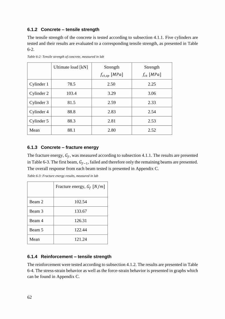
62
6.1.2 Concrete – tensile strength
The tensile strength of the concrete is tested according to subsection 4.1.1. Five cylinders are
tested and their results are evaluated to a corresponding tensile strength, as presented in Table
6-2.
Table 6-2: Tensile strength of concrete, measured in lab
Ultimate load [kN] Strength
𝑓𝑐𝑡,𝑠𝑝 [𝑀𝑃𝑎]
Strength
𝑓𝑐𝑡 [𝑀𝑃𝑎]
Cylinder 1 78.5 2.50 2.25
Cylinder 2 103.4 3.29 3.06
Cylinder 3 81.5 2.59 2.33
Cylinder 4 88.8 2.83 2.54
Cylinder 5 88.3 2.81 2.53
Mean 88.1 2.80 2.52
6.1.3 Concrete – fracture energy
The fracture energy, 𝐺𝑓, was measured according to subsection 4.1.1. The results are presented
in Table 6-3. The first beam, 𝐺𝑓−1, failed and therefore only the remaining beams are presented.
The overall response from each beam tested is presented in Appendix C.
Table 6-3: Fracture energy results, measured in lab
Fracture energy, 𝐺𝑓 [𝑁/𝑚]
Beam 2 102.54
Beam 3 133.67
Beam 4 126.31
Beam 5 122.44
Mean 121.24
6.1.4 Reinforcement – tensile strength
The reinforcement were tested according to subsection 4.1.2. The results are presented in Table
6-4. The stress-strain behavior as well as the force-strain behavior is presented in graphs which
can be found in Appendix C.
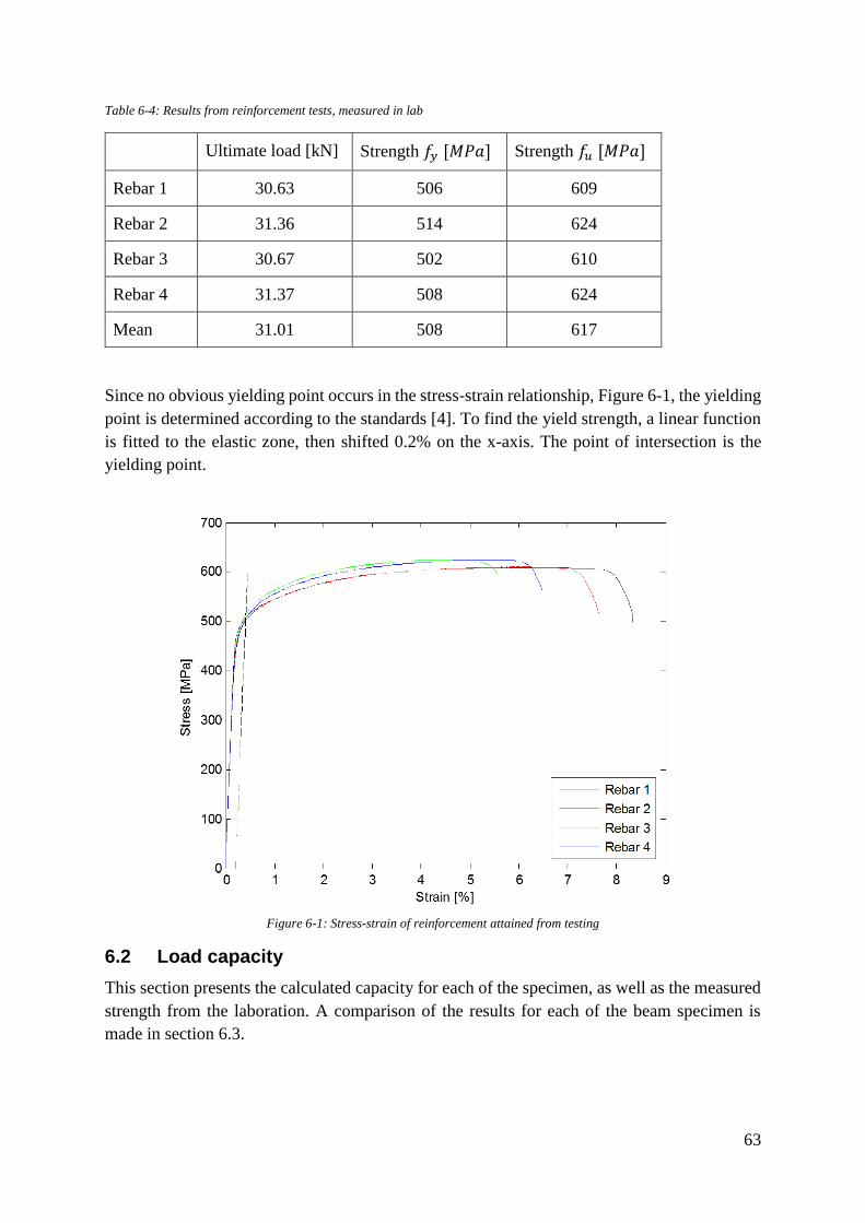
63
Table 6-4: Results from reinforcement tests, measured in lab
Ultimate load [kN] Strength 𝑓𝑦 [𝑀𝑃𝑎] Strength 𝑓𝑢 [𝑀𝑃𝑎]
Rebar 1 30.63 506 609
Rebar 2 31.36 514 624
Rebar 3 30.67 502 610
Rebar 4 31.37 508 624
Mean 31.01 508 617
Since no obvious yielding point occurs in the stress-strain relationship, Figure 6-1, the yielding
point is determined according to the standards [4]. To find the yield strength, a linear function
is fitted to the elastic zone, then shifted 0.2% on the x-axis. The point of intersection is the
yielding point.
Figure 6-1: Stress-strain of reinforcement attained from testing
6.2 Load capacity
This section presents the calculated capacity for each of the specimen, as well as the measured
strength from the laboration. A comparison of the results for each of the beam specimen is
made in section 6.3.
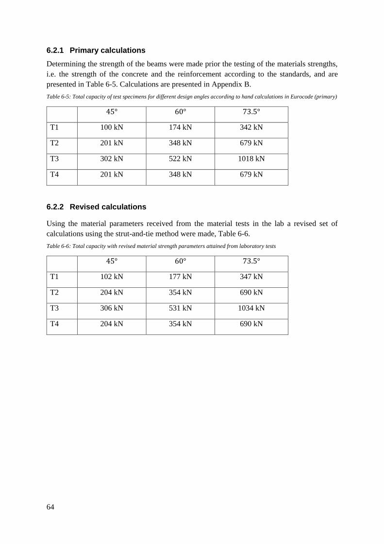
64
6.2.1 Primary calculations
Determining the strength of the beams were made prior the testing of the materials strengths,
i.e. the strength of the concrete and the reinforcement according to the standards, and are
presented in Table 6-5. Calculations are presented in Appendix B.
Table 6-5: Total capacity of test specimens for different design angles according to hand calculations in Eurocode (primary)
45° 60° 73.5°
T1 100 kN 174 kN 342 kN
T2 201 kN 348 kN 679 kN
T3 302 kN 522 kN 1018 kN
T4 201 kN 348 kN 679 kN
6.2.2 Revised calculations
Using the material parameters received from the material tests in the lab a revised set of
calculations using the strut-and-tie method were made, Table 6-6.
Table 6-6: Total capacity with revised material strength parameters attained from laboratory tests
45° 60° 73.5°
T1 102 kN 177 kN 347 kN
T2 204 kN 354 kN 690 kN
T3 306 kN 531 kN 1034 kN
T4 204 kN 354 kN 690 kN
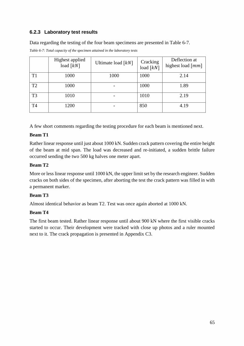
65
6.2.3 Laboratory test results
Data regarding the testing of the four beam specimens are presented in Table 6-7.
Table 6-7: Total capacity of the specimen attained in the laboratory tests
Highest applied
load [𝑘𝑁] Ultimate load [𝑘𝑁] Cracking
load [𝑘𝑁]
Deflection at
highest load [𝑚𝑚]
T1 1000 1000 1000 2.14
T2 1000 - 1000 1.89
T3 1010 - 1010 2.19
T4 1200 - 850 4.19
A few short comments regarding the testing procedure for each beam is mentioned next.
Beam T1
Rather linear response until just about 1000 kN. Sudden crack pattern covering the entire height
of the beam at mid span. The load was decreased and re-initiated, a sudden brittle failure
occurred sending the two 500 kg halves one meter apart.
Beam T2
More or less linear response until 1000 kN, the upper limit set by the research engineer. Sudden
cracks on both sides of the specimen, after aborting the test the crack pattern was filled in with
a permanent marker.
Beam T3
Almost identical behavior as beam T2. Test was once again aborted at 1000 kN.
Beam T4
The first beam tested. Rather linear response until about 900 kN where the first visible cracks
started to occur. Their development were tracked with close up photos and a ruler mounted
next to it. The crack propagation is presented in Appendix C3.
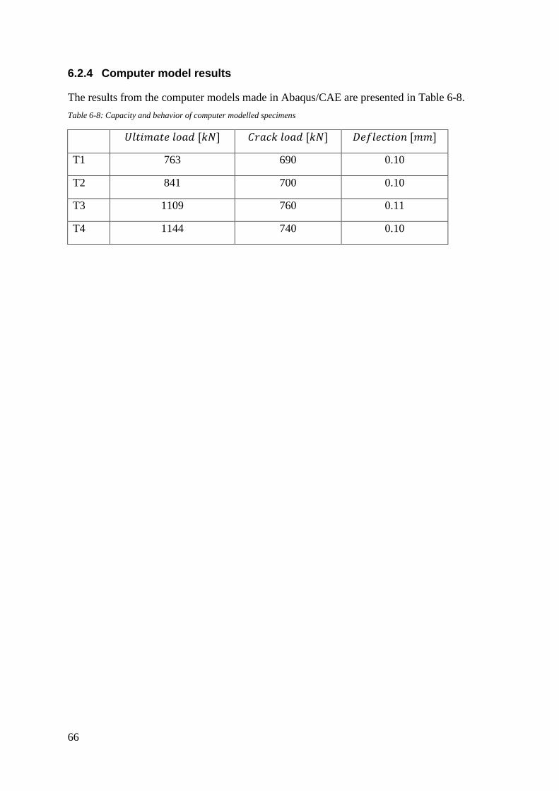
66
6.2.4 Computer model results
The results from the computer models made in Abaqus/CAE are presented in Table 6-8.
Table 6-8: Capacity and behavior of computer modelled specimens
𝑈𝑙𝑡𝑖𝑚𝑎𝑡𝑒 𝑙𝑜𝑎𝑑 [𝑘𝑁] 𝐶𝑟𝑎𝑐𝑘 𝑙𝑜𝑎𝑑 [𝑘𝑁] 𝐷𝑒𝑓𝑙𝑒𝑐𝑡𝑖𝑜𝑛 [𝑚𝑚]
T1 763 690 0.10
T2 841 700 0.10
T3 1109 760 0.11
T4 1144 740 0.10
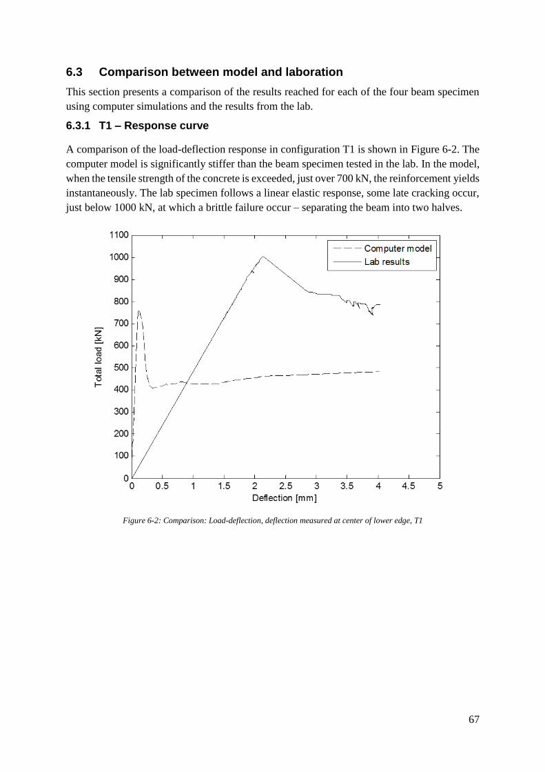
67
6.3 Comparison between model and laboration
This section presents a comparison of the results reached for each of the four beam specimen
using computer simulations and the results from the lab.
6.3.1 T1 – Response curve
A comparison of the load-deflection response in configuration T1 is shown in Figure 6-2. The
computer model is significantly stiffer than the beam specimen tested in the lab. In the model,
when the tensile strength of the concrete is exceeded, just over 700 kN, the reinforcement yields
instantaneously. The lab specimen follows a linear elastic response, some late cracking occur,
just below 1000 kN, at which a brittle failure occur – separating the beam into two halves.
Figure 6-2: Comparison: Load-deflection, deflection measured at center of lower edge, T1
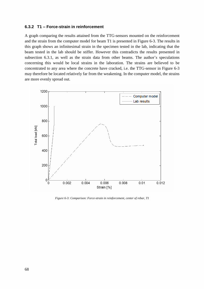
68
6.3.2 T1 – Force-strain in reinforcement
A graph comparing the results attained from the TTG-sensors mounted on the reinforcement
and the strain from the computer model for beam T1 is presented in Figure 6-3. The results in
this graph shows an infinitesimal strain in the specimen tested in the lab, indicating that the
beam tested in the lab should be stiffer. However this contradicts the results presented in
subsection 6.3.1, as well as the strain data from other beams. The author’s speculations
concerning this would be local strains in the laboration. The strains are believed to be
concentrated to any area where the concrete have cracked, i.e. the TTG-sensor in Figure 6-3
may therefore be located relatively far from the weakening. In the computer model, the strains
are more evenly spread out.
Figure 6-3: Comparison: Force-strain in reinforcement, center of rebar, T1
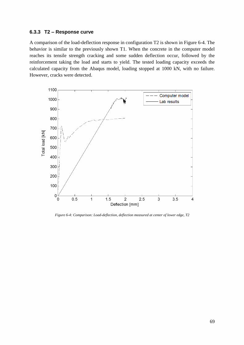
69
6.3.3 T2 – Response curve
A comparison of the load-deflection response in configuration T2 is shown in Figure 6-4. The
behavior is similar to the previously shown T1. When the concrete in the computer model
reaches its tensile strength cracking and some sudden deflection occur, followed by the
reinforcement taking the load and starts to yield. The tested loading capacity exceeds the
calculated capacity from the Abaqus model, loading stopped at 1000 kN, with no failure.
However, cracks were detected.
Figure 6-4: Comparison: Load-deflection, deflection measured at center of lower edge, T2
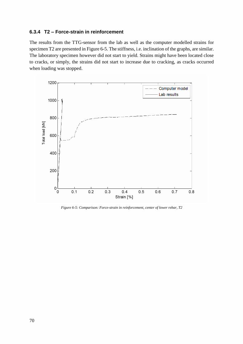
70
6.3.4 T2 – Force-strain in reinforcement
The results from the TTG-sensor from the lab as well as the computer modelled strains for
specimen T2 are presented in Figure 6-5. The stiffness, i.e. inclination of the graphs, are similar.
The laboratory specimen however did not start to yield. Strains might have been located close
to cracks, or simply, the strains did not start to increase due to cracking, as cracks occurred
when loading was stopped.
Figure 6-5: Comparison: Force-strain in reinforcement, center of lower rebar, T2
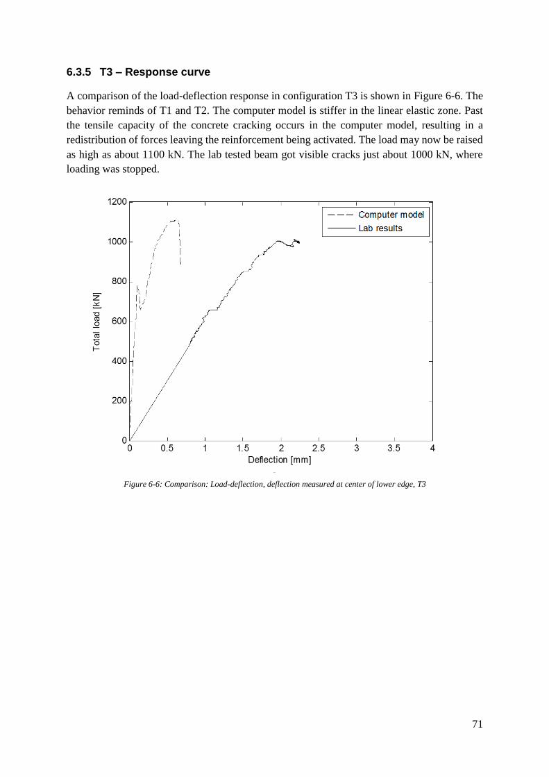
71
6.3.5 T3 – Response curve
A comparison of the load-deflection response in configuration T3 is shown in Figure 6-6. The
behavior reminds of T1 and T2. The computer model is stiffer in the linear elastic zone. Past
the tensile capacity of the concrete cracking occurs in the computer model, resulting in a
redistribution of forces leaving the reinforcement being activated. The load may now be raised
as high as about 1100 kN. The lab tested beam got visible cracks just about 1000 kN, where
loading was stopped.
Figure 6-6: Comparison: Load-deflection, deflection measured at center of lower edge, T3
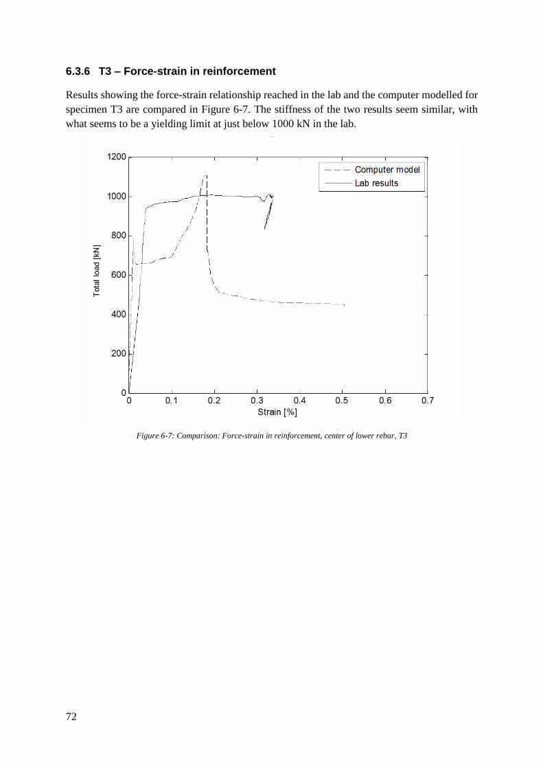
72
6.3.6 T3 – Force-strain in reinforcement
Results showing the force-strain relationship reached in the lab and the computer modelled for
specimen T3 are compared in Figure 6-7. The stiffness of the two results seem similar, with
what seems to be a yielding limit at just below 1000 kN in the lab.
Figure 6-7: Comparison: Force-strain in reinforcement, center of lower rebar, T3
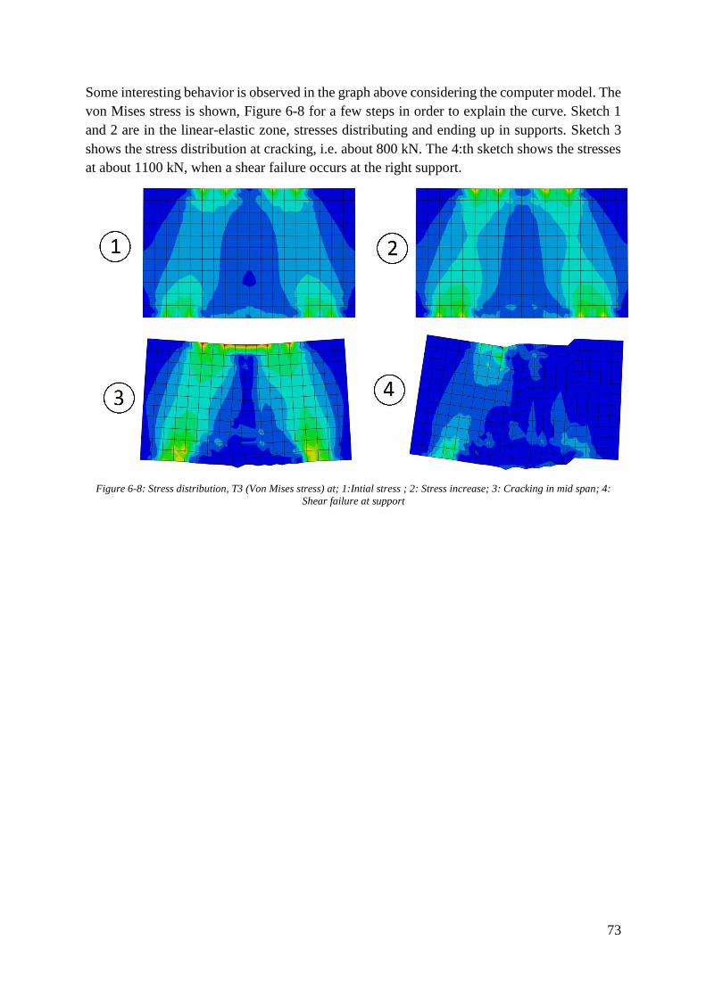
73
Some interesting behavior is observed in the graph above considering the computer model. The
von Mises stress is shown, Figure 6-8 for a few steps in order to explain the curve. Sketch 1
and 2 are in the linear-elastic zone, stresses distributing and ending up in supports. Sketch 3
shows the stress distribution at cracking, i.e. about 800 kN. The 4:th sketch shows the stresses
at about 1100 kN, when a shear failure occurs at the right support.
Figure 6-8: Stress distribution, T3 (Von Mises stress) at; 1:Intial stress ; 2: Stress increase; 3: Cracking in mid span; 4:
Shear failure at support
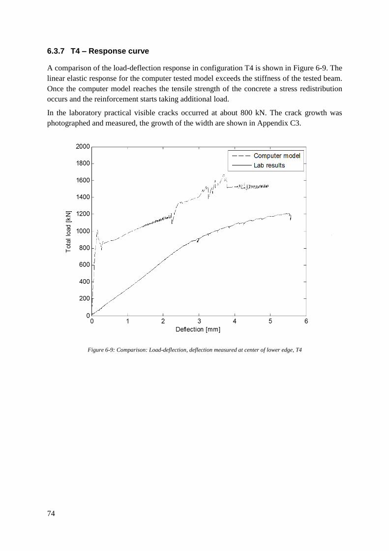
74
6.3.7 T4 – Response curve
A comparison of the load-deflection response in configuration T4 is shown in Figure 6-9. The
linear elastic response for the computer tested model exceeds the stiffness of the tested beam.
Once the computer model reaches the tensile strength of the concrete a stress redistribution
occurs and the reinforcement starts taking additional load.
In the laboratory practical visible cracks occurred at about 800 kN. The crack growth was
photographed and measured, the growth of the width are shown in Appendix C3.
Figure 6-9: Comparison: Load-deflection, deflection measured at center of lower edge, T4
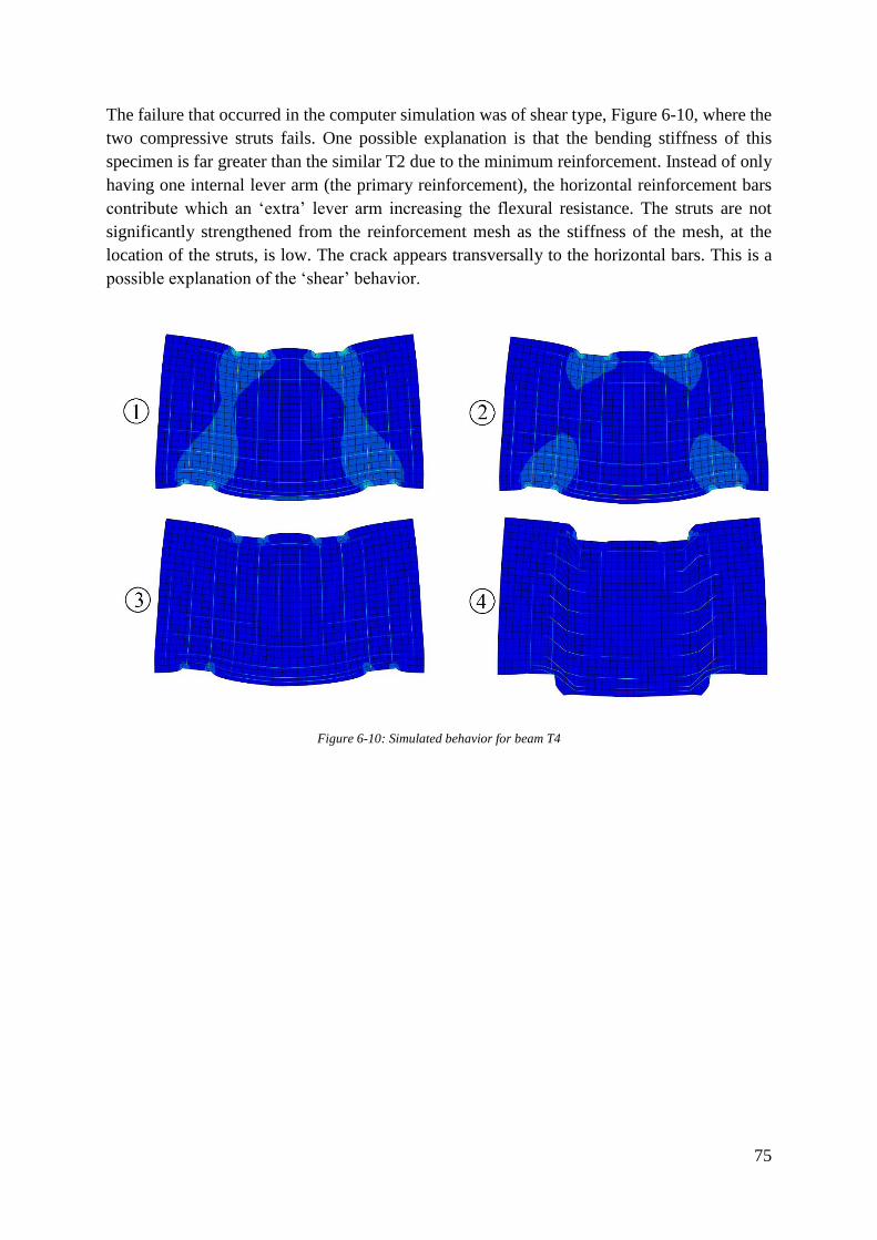
75
The failure that occurred in the computer simulation was of shear type, Figure 6-10, where the
two compressive struts fails. One possible explanation is that the bending stiffness of this
specimen is far greater than the similar T2 due to the minimum reinforcement. Instead of only
having one internal lever arm (the primary reinforcement), the horizontal reinforcement bars
contribute which an ‘extra’ lever arm increasing the flexural resistance. The struts are not
significantly strengthened from the reinforcement mesh as the stiffness of the mesh, at the
location of the struts, is low. The crack appears transversally to the horizontal bars. This is a
possible explanation of the ‘shear’ behavior.
Figure 6-10: Simulated behavior for beam T4
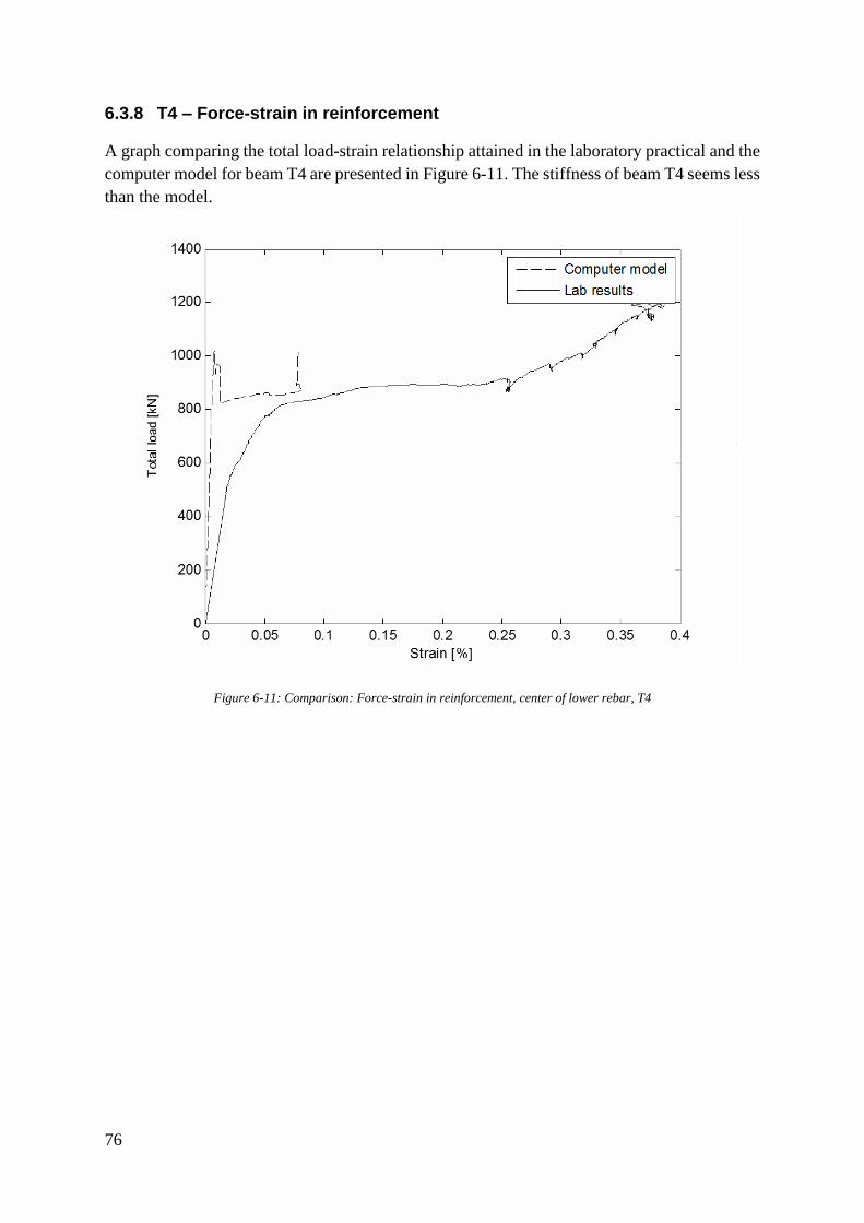
76
6.3.8 T4 – Force-strain in reinforcement
A graph comparing the total load-strain relationship attained in the laboratory practical and the
computer model for beam T4 are presented in Figure 6-11. The stiffness of beam T4 seems less
than the model.
Figure 6-11: Comparison: Force-strain in reinforcement, center of lower rebar, T4
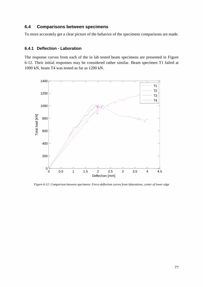
77
6.4 Comparisons between specimens
To more accurately get a clear picture of the behavior of the specimens comparisons are made.
6.4.1 Deflection - Laboration
The response curves from each of the in lab tested beam specimens are presented in Figure
6-12. Their initial responses may be considered rather similar. Beam specimen T1 failed at
1000 kN, beam T4 was tested as far as 1200 kN.
Figure 6-12: Comparison between specimens: Force-deflection curves from laborations, center of lower edge
0 0.5 1 1.5 2 2.5 3 3.5 4 4.50
200
400
600
800
1000
1200
1400
Deflection [mm]
Tota
l lo
ad [
kN
]
T1
T2
T3
T4
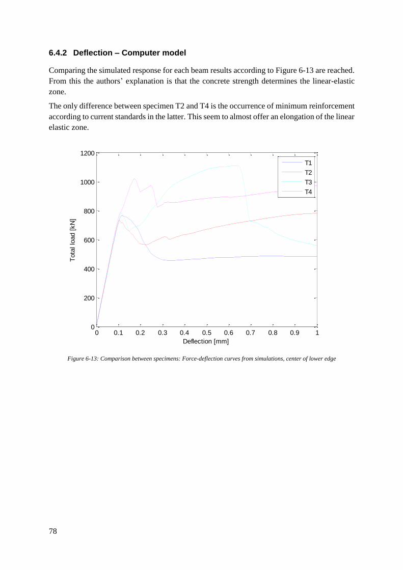
78
6.4.2 Deflection – Computer model
Comparing the simulated response for each beam results according to Figure 6-13 are reached.
From this the authors’ explanation is that the concrete strength determines the linear-elastic
zone.
The only difference between specimen T2 and T4 is the occurrence of minimum reinforcement
according to current standards in the latter. This seem to almost offer an elongation of the linear
elastic zone.
Figure 6-13: Comparison between specimens: Force-deflection curves from simulations, center of lower edge
0 0.1 0.2 0.3 0.4 0.5 0.6 0.7 0.8 0.9 10
200
400
600
800
1000
1200
Deflection [mm]
Tota
l lo
ad [
kN
]
T1
T2
T3
T4
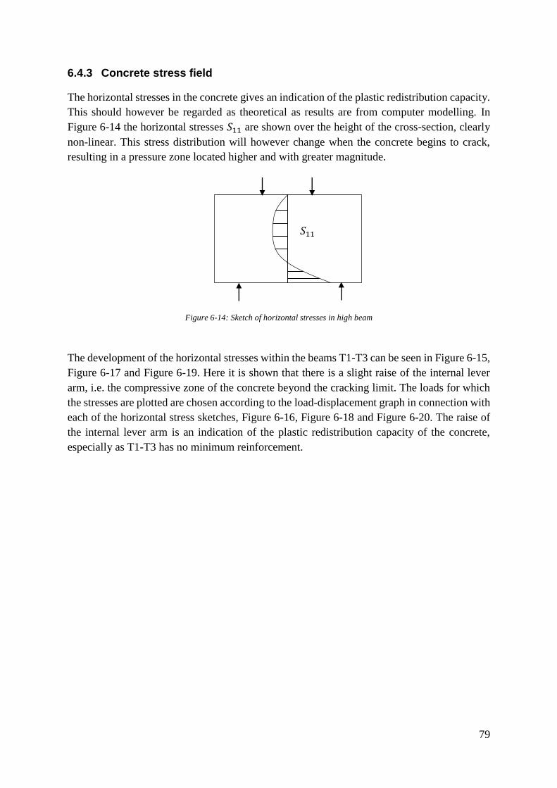
79
6.4.3 Concrete stress field
The horizontal stresses in the concrete gives an indication of the plastic redistribution capacity.
This should however be regarded as theoretical as results are from computer modelling. In
Figure 6-14 the horizontal stresses 𝑆11 are shown over the height of the cross-section, clearly
non-linear. This stress distribution will however change when the concrete begins to crack,
resulting in a pressure zone located higher and with greater magnitude.
Figure 6-14: Sketch of horizontal stresses in high beam
The development of the horizontal stresses within the beams T1-T3 can be seen in Figure 6-15,
Figure 6-17 and Figure 6-19. Here it is shown that there is a slight raise of the internal lever
arm, i.e. the compressive zone of the concrete beyond the cracking limit. The loads for which
the stresses are plotted are chosen according to the load-displacement graph in connection with
each of the horizontal stress sketches, Figure 6-16, Figure 6-18 and Figure 6-20. The raise of
the internal lever arm is an indication of the plastic redistribution capacity of the concrete,
especially as T1-T3 has no minimum reinforcement.
𝑆11
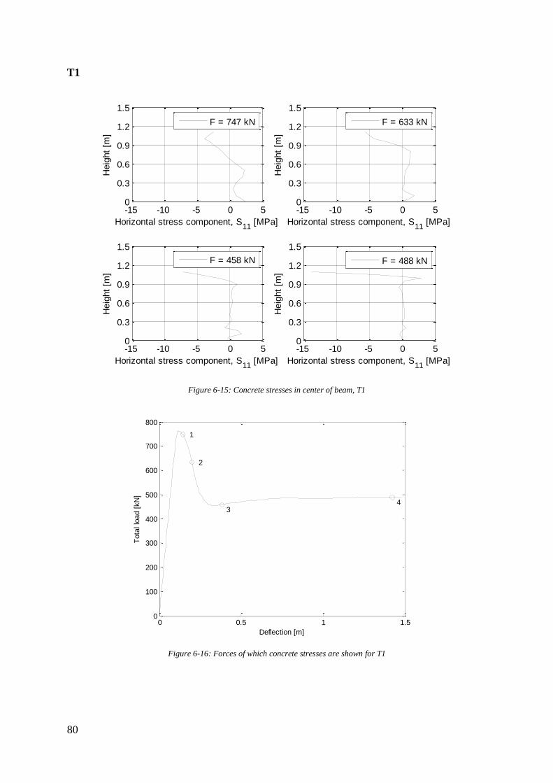
80
T1
Figure 6-15: Concrete stresses in center of beam, T1
Figure 6-16: Forces of which concrete stresses are shown for T1
-15 -10 -5 0 50
0.3
0.6
0.9
1.2
1.5
Horizontal stress component, S11
[MPa]
Heig
ht
[m]
F = 747 kN
-15 -10 -5 0 50
0.3
0.6
0.9
1.2
1.5
Horizontal stress component, S11
[MPa]
Heig
ht
[m]
F = 633 kN
-15 -10 -5 0 50
0.3
0.6
0.9
1.2
1.5
Horizontal stress component, S11
[MPa]
Heig
ht
[m]
F = 458 kN
-15 -10 -5 0 50
0.3
0.6
0.9
1.2
1.5
Horizontal stress component, S11
[MPa]
Heig
ht
[m]
F = 488 kN
0 0.5 1 1.50
100
200
300
400
500
600
700
800
1
2
3
4
Deflection [m]
Tota
l lo
ad [
kN
]
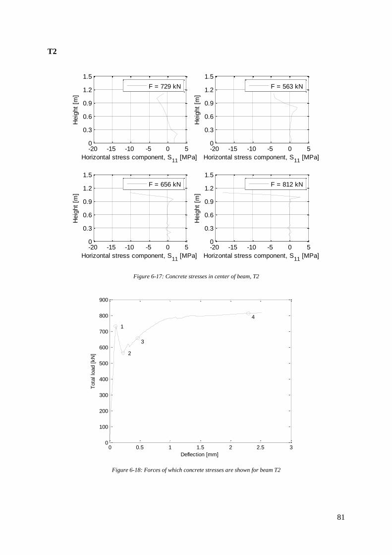
81
T2
Figure 6-17: Concrete stresses in center of beam, T2
Figure 6-18: Forces of which concrete stresses are shown for beam T2
-20 -15 -10 -5 0 50
0.3
0.6
0.9
1.2
1.5
Horizontal stress component, S11
[MPa]
Heig
ht
[m]
F = 729 kN
-20 -15 -10 -5 0 50
0.3
0.6
0.9
1.2
1.5
Horizontal stress component, S11
[MPa]
Heig
ht
[m]
F = 563 kN
-20 -15 -10 -5 0 50
0.3
0.6
0.9
1.2
1.5
Horizontal stress component, S11
[MPa]
Heig
ht
[m]
F = 656 kN
-20 -15 -10 -5 0 50
0.3
0.6
0.9
1.2
1.5
Horizontal stress component, S11
[MPa]
Heig
ht
[m]
F = 812 kN
0 0.5 1 1.5 2 2.5 30
100
200
300
400
500
600
700
800
900
1
2
3
4
Deflection [mm]
Tota
l lo
ad [
kN
]
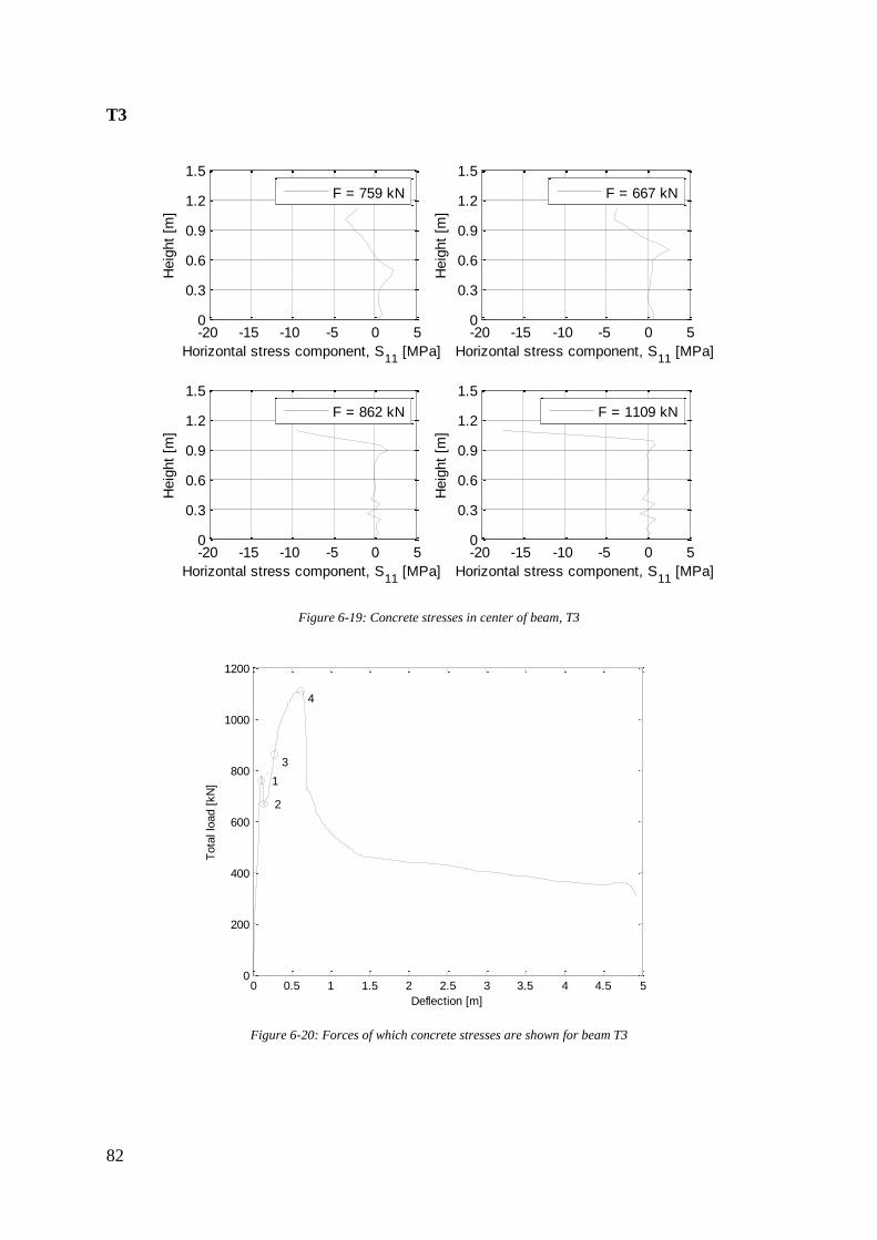
82
T3
Figure 6-19: Concrete stresses in center of beam, T3
Figure 6-20: Forces of which concrete stresses are shown for beam T3
-20 -15 -10 -5 0 50
0.3
0.6
0.9
1.2
1.5
Horizontal stress component, S11
[MPa]
Heig
ht
[m]
F = 759 kN
-20 -15 -10 -5 0 50
0.3
0.6
0.9
1.2
1.5
Horizontal stress component, S11
[MPa]
Heig
ht
[m]
F = 667 kN
-20 -15 -10 -5 0 50
0.3
0.6
0.9
1.2
1.5
Horizontal stress component, S11
[MPa]
Heig
ht
[m]
F = 862 kN
-20 -15 -10 -5 0 50
0.3
0.6
0.9
1.2
1.5
Horizontal stress component, S11
[MPa]
Heig
ht
[m]
F = 1109 kN
0 0.5 1 1.5 2 2.5 3 3.5 4 4.5 50
200
400
600
800
1000
1200
1
2
3
4
Deflection [m]
Tota
l lo
ad [
kN
]
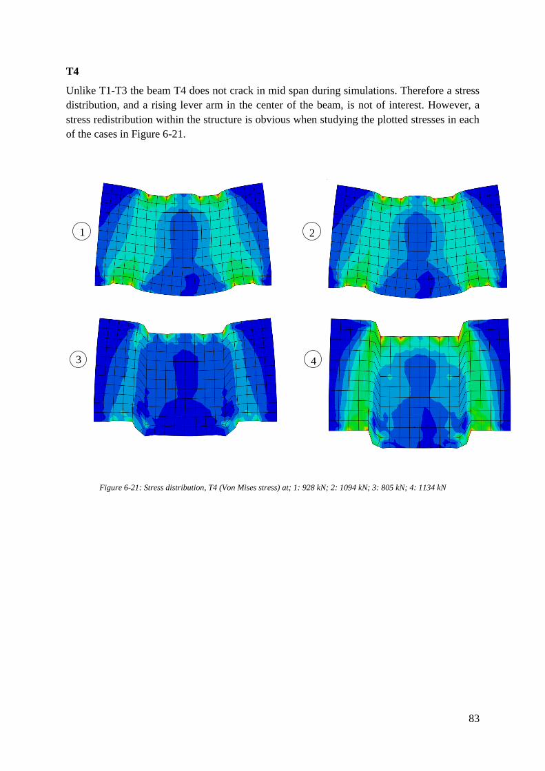
83
T4
Unlike T1-T3 the beam T4 does not crack in mid span during simulations. Therefore a stress
distribution, and a rising lever arm in the center of the beam, is not of interest. However, a
stress redistribution within the structure is obvious when studying the plotted stresses in each
of the cases in Figure 6-21.
Figure 6-21: Stress distribution, T4 (Von Mises stress) at; 1: 928 kN; 2: 1094 kN; 3: 805 kN; 4: 1134 kN
1 2
3 4
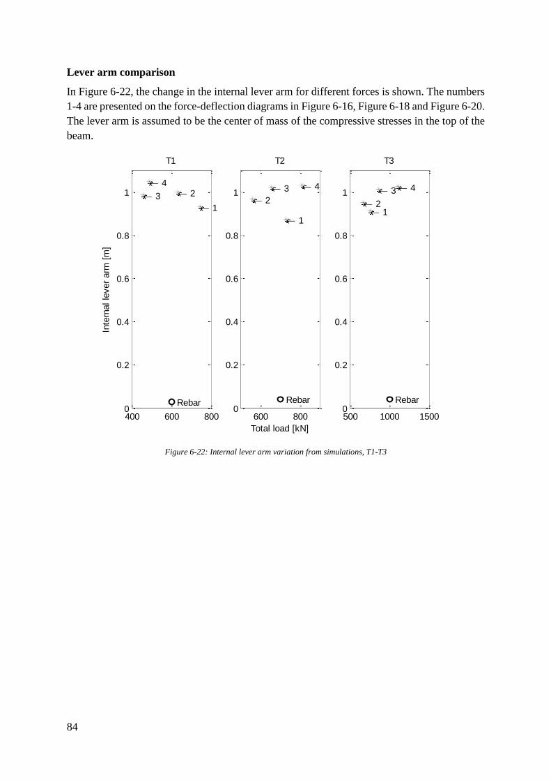
84
Lever arm comparison
In Figure 6-22, the change in the internal lever arm for different forces is shown. The numbers
1-4 are presented on the force-deflection diagrams in Figure 6-16, Figure 6-18 and Figure 6-20.
The lever arm is assumed to be the center of mass of the compressive stresses in the top of the
beam.
Figure 6-22: Internal lever arm variation from simulations, T1-T3
400 600 8000
0.2
0.4
0.6
0.8
1
T1
1
2 3
4
Rebar
Inte
rnal le
ver
arm
[m
]
600 8000
0.2
0.4
0.6
0.8
1
T2
1
2
3 4
Rebar
Total load [kN]
500 1000 15000
0.2
0.4
0.6
0.8
1
T3
1 2
3 4
Rebar
85
6.5 Discussion
Some difficulties encountered in the project are discussed below. They are divided in lab- and
computer related difficulties.
Laboratory practical
The small number of specimen leave a high insecurity in all results, since a large
number of differences between specimen are possible. A larger number of tests would
be preferable, but not realistic due to the size.
Tensile strength of the concrete may be inconsistent. The theoretical tensile strength
assumes the weakest link to be situated along the perimeter. Most tensile weaknesses
are overlooked in a ‘compressive test of the tensile strength’ since cracks and other
weaknesses are compressed and stabilized rather than exploited. A direct tensile test
would have been preferable.
Inaccurate measurements are unfortunately a major source of potential errors. Both in
terms of the hydraulic load readings but also the deflections gauges (LVDT). For
example some values from the LVDT’s proved to be useless. A calibration was made
whenever possible. There are also questions whether the deflection of the beam was
properly measured.
The casts were more or less identical in size when built, but at casting the horizontal
pressure deformed the casts resulting in noticeable, but small, non-uniformities between
the beam specimens. As a result of the risk of mold collapse, the vibration of the
concrete may have been insufficient.
Placement of the reinforcement bars is easily done in theory but difficult in practice.
Small deviations have been made, since accuracy within millimeters is difficult to
achieve, but the results should not be affected.
In the initial steps of each test the system were ‘compacted’ prior the linear response of
the beam. For example the dry cement applied on top. To compensate for this a linear
approximation was made backwards. This linear approximation is sensitive to the
choice of starting point selected and may give misleading results.
In the design of the tests the authors chose to be conservative, e.g. using safety factors
when calculating strut and node capacities. This resulted in a wide beam, with high
concrete capacity. This lead to a very high crack-inducing load.
Computer simulation
The number of parameters needed to model the beams in BRIGADE/Plus are
overwhelming and the background theory is complex. The parameters which were not
determined in the lab, i.e. the ‘viscosity parameter’, ‘dilation angle’, ‘K’, ‘fb0/fc0’ and
the ‘eccentricity’, was either taken as the default value or from literature. Whether or
not the values are good is difficult to tell.
86
To determine the Young’s modulus of the concrete it would have been more accurate
to test a specimen in the hydraulic MTS. Even though it would not have been able to
press the specimen to failure, the Young’s modulus for the elastic zone would have
been retrieved, rather than evaluating it according to the codes.
The Young’s modulus in the reinforcement bars might be too high. Sliding in the
machine might yield misleading results. Also, the choice of the points on the graph for
which Young’s modulus may change the result.
87
7 CONCLUSIONS
7.1 Conclusions from work
1. When using the strut-and-tie method the tensile strength of the concrete as well as the
strength of the minimum reinforcement is neglected. Questions may in some cases be
raised whether or not this is accurate. Some analysis should also be done to check at
which load the concrete starts to crack – as the strut-and-tie method models cracked
behavior.
2. To assess a beam according to the strut-and-tie method it is important to understand the
importance of crack behavior. To properly calculate the cracking load, a finite element
analysis should be performed. Calculating cracking load according to basic beam theory
gave a cracking load of about 338 𝑘𝑁, lower than the capacity of the weakest beam. A
calculation replacing the tie consisting of reinforcement bars with a tie consisting of
concrete, using the geometry given from node capacity calculations, gave a cracking
load of about 296 kN. These simplifications are obviously not accurate.
3. Load bearing capacity calculations for the least reinforced beam, T1, according to the
strut-and-tie model might be correct. The sudden, brittle, failure might be explained by
the tensile capacity of the concrete. The capacity specimen T1 would have reached in
the ultimate limit state, at yielding of the reinforcement, is less than the load required
to induce cracks. When the first crack propagated, strains probably localized near the
crack, and in this particular area the strength of the reinforcement bar was exceeded.
When designing, a brittle failure should be avoided.
4. When evaluating failures of the tested beam specimens there are roughly two types of
behavior. Those are; the brittle behavior of beam T1 and the ductile behavior of beam
T4. T1 actually gave a stiffer response compared to the ductile beam T4. However,
when failure occurred in beam T1 it was sudden and powerful. A structural element
with such behavior would be dangerous to say the least. Therefore, it seems well
motivated to use minimum reinforcement. Another advantage using minimum
reinforcement is the reduction of crack widths. Studying Appendix D one may realize
the increased number of cracks, but in theory they should be thinner compared to one
single crack.
5. Laboratory results gave higher deflections than the computer model. Since all beams in
laboratory and all beams in computer modelling showed similar force-deflection
behavior, the errors probably were systematic. Therefore, some comparisons within
modelling or laboratory work are valid. The cause of the differences has not been
identified. Probably, a systematic measurement error exists, as the model should
capture the behavior correctly in the linear-elastic stage. The results of the model might
also be wrong, over-estimating the stiffness.
88
6. One of the scopes of the project, to investigate whether there exists a plastic
redistribution capacity of the concrete specimen which might yield a higher design
angles, cannot be determined. There exists indications from laboratory work in
specimen T4. There is a contribution from the minimum reinforcement to the ductile
behavior and redistribution ability, but as structures in reality always (at least when
designing according to Eurocode) are constructed with minimum reinforcement, there
are indications of a low design angle being over-conservative and that the structure has
an ability to redistribute stresses. The computer models indicates a stress redistribution
capacity.
7.2 Further research
Firstly, because of the some difficulties were encountered, further research with higher
consideration for these difficulties and problems could yield more comparable results. Some
suggestions are listed:
In order to load the beams to failure a load distribution beam could be used. This may
be placed on the rolling plate and positioned under the press, enabling a higher
maximum force.
Having smaller dimensions, more test specimens may be manufactured and tested
which increases the reliability of the results.
Measure deflections directly from an independent reference point, instead of measuring
deformations indirectly including deformations of the wagon.
Secondly, the whole design of the test could be more relevant in terms of comparing reality
and theory. Some suggestions are listed:
If possible use uniformly distributed loading instead of two-point loading, as this
corresponds to the most common load case.
As minimum reinforcement is used in reality, this could be included in all specimens.
Thirdly, there are several interesting aspects to study in relation to the strut-and-tie method.
Some suggestions are listed:
Whether the contribution of minimum reinforcement to load-bearing capacity should
be considered or not when regarding ultimate limit state is often debated. A study
focusing on how this reinforcement affects ultimate limit state and serviceability limit
state, and whether plastic redistribution in the concrete could actually be accounted for,
might be interesting.
Investigation of the use of fiber reinforcement instead of minimum reinforcement mesh,
as it decreases time spent on placement of reinforcement and thereby work in situ.
Aspects of interest are serviceability limit state (i.e. crack widths) and ductility
compared to the use of minimum reinforcement mesh.
89
A study on how different material parameters affects crack-growth in high concrete
members. As designing according to the strut-and-tie method might make use of a large
stress redistribution due to cracking, proper crack behavior is important to capture. A
suggestion is to measure different material parameters included in a model, e.g.
Concrete Damaged Plasticity, and how these affects model performance compared to
real tests.

90
91
REFERENCES
[1] I. S. Newton, Philosophie Naturalis Principia Mathematica, London: Benediction
Classics, 1687.
[2] W.-F. Chen, Plasticity in reinforced concrete, -: McGraw-Hill Inc., 1982.
[3] P. G. Burström, Byggnadsmaterial, Uppbyggnad, tillverkning och egenskaper, Pozkal:
Studentlitteratur, 2007.
[4] Swedish Standard Institute, "Svensk standard SS-EN 1992-1-1:2005," SIS Förlag,
Stockholm, 2008.
[5] A. M. Neville, Properties of Concrete, Longman Group Ltd, 1995.
[6] W.-F. Chen and D.-J. Han, Plasticity for Structural Engineers, New York: Springer-
Verlag, 1988.
[7] P. K. Mehta, Concrete structure, properties, and materials, New Jersey: Prentice-Hall
Inc., 1986.
[8] B. Engström, "Design and analysis of deep beams, plates and other discontinuity
regions," Chalmers, Göteborg, 2011.
[9] T. Isaksson and A. Mårtensson, Byggkonstruktion Regel- och formelsamling, Lund:
Studentlitteratur, 2010.
[10] J. Schlaich, K. Schäfer and M. Jennewein, "Toward a Consistent Design of Structural
Concrete," Presstressed concrete institute, Stuttgart, -.
[11] N. Saabye Ottosen and H. Petersson, Introduction to the finite element method, Bungay:
Prentice Hall Europe, 1992.
[12] A. Hillerborg, "Application of Fracture Mechanics to Concrete," Lund, 1988.
[13] R. Malm, "Shear cracks in concrete structures subjected to in-plane stresses," Royal
Institute of Technology (KTH), Stockholm, 2006.
[14] A. Hillerborg, "The theoretical basis of a method to determine the fracutre energy Gf of
concrete," Rilem Technical Committees, Lund, 1985.
[15] R. Malm, Predicting shear type crack initiation and growth in concrete with non-linear
finite element method, Stockholm: Royal Institute of Technology (KTH), 2009.
92
[16] H. Hibbitt, B. Karlsson and E. Sorensen, ABAQUS version 6.7 finite element program -
standard user's manual, 2007.
[17] Dassault Systèmes, "Abaqus/CAE Users's Guide," Dassault Systèms Simulia Corp,
Providence, 2013.
[18] J. Lubliner, J. Oliver, S. Oller and E. Oñate, "A Plastic-Damage Model for Concrete,"
International Journal of Solids and Structures, pp. 299-326, 6 April 1989.
[19] Building Research Institute, "Material Testing," Building Research Institute, [Online].
Available: http://www.buildingresearch.com.np/services/mt/mt2.php. [Accessed 08 02
2016].
[20] P. Bamforth, D. Chisholm, J. Gibbs and T. Harrison, "Properties of Concrete for use in
Eurocode 2," The Concrete Centre, Camberley, 2008.
[21] J. Malvar and G. Warren, "Fracture Energy for Three-Point Bend Tests on Single-Edge
Notched Beams," NCEL Technical Report, Port Hueneme, 1988.
[22] M. Szcecina and A. Winnicki, "Calibration of the CDP model parameters in Abaqus,"
The 2015 World Congress on Advances in Structural Engineering and MEchanics
(ASEM15), Incheon, 2015.

93
APPENDIX A - DRAWINGS
This Appendix contains drawings for each of the beam configurations used. The drawings
included are:
A1 – Beam T1
A2 – Beam T2
A3 – Beam T3
A4 – Beam T4
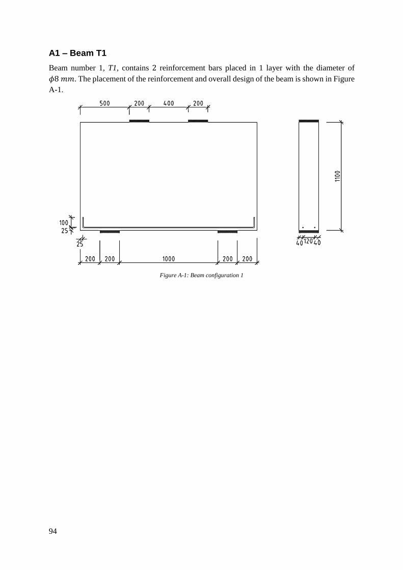
94
A1 – Beam T1
Beam number 1, T1, contains 2 reinforcement bars placed in 1 layer with the diameter of
𝜙8 𝑚𝑚. The placement of the reinforcement and overall design of the beam is shown in Figure
A-1.
Figure A-1: Beam configuration 1
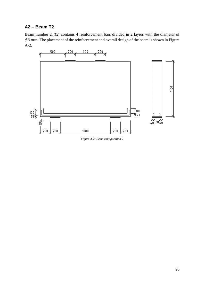
95
A2 – Beam T2
Beam number 2, T2, contains 4 reinforcement bars divided in 2 layers with the diameter of
𝜙8 𝑚𝑚. The placement of the reinforcement and overall design of the beam is shown in Figure
A-2.
Figure A-2: Beam configuration 2
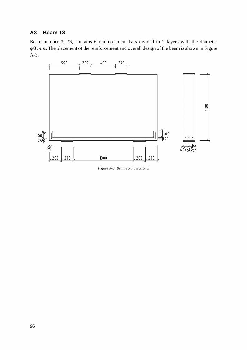
96
A3 – Beam T3
Beam number 3, T3, contains 6 reinforcement bars divided in 2 layers with the diameter
𝜙8 𝑚𝑚. The placement of the reinforcement and overall design of the beam is shown in Figure
A-3.
Figure A-3: Beam configuration 3
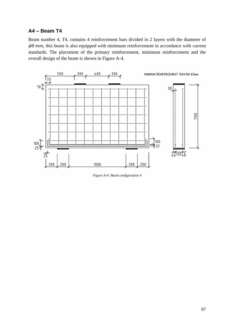
97
A4 – Beam T4
Beam number 4, T4, contains 4 reinforcement bars divided in 2 layers with the diameter of
𝜙8 𝑚𝑚, this beam is also equipped with minimum reinforcement in accordance with current
standards. The placement of the primary reinforcement, minimum reinforcement and the
overall design of the beam is shown in Figure A-4.
Figure A-4: Beam configuration 4

98
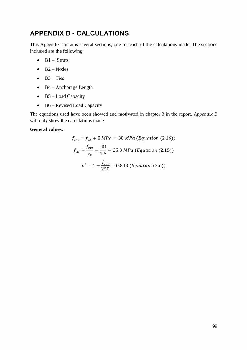
99
APPENDIX B - CALCULATIONS
This Appendix contains several sections, one for each of the calculations made. The sections
included are the following:
B1 – Struts
B2 – Nodes
B3 – Ties
B4 – Anchorage Length
B5 – Load Capacity
B6 – Revised Load Capacity
The equations used have been showed and motivated in chapter 3 in the report. Appendix B
will only show the calculations made.
General values:
𝑓𝑐𝑚 = 𝑓𝑐𝑘 + 8 𝑀𝑃𝑎 = 38 𝑀𝑃𝑎 (𝐸𝑞𝑢𝑎𝑡𝑖𝑜𝑛 (2.16))
𝑓𝑐𝑑 =𝑓𝑐𝑚
𝛾𝐶=
38
1.5= 25.3 𝑀𝑃𝑎 (𝐸𝑞𝑢𝑎𝑡𝑖𝑜𝑛 (2.15))
𝑣′ = 1 −𝑓𝑐𝑚
250= 0.848 (𝐸𝑞𝑢𝑎𝑡𝑖𝑜𝑛 (3.6))
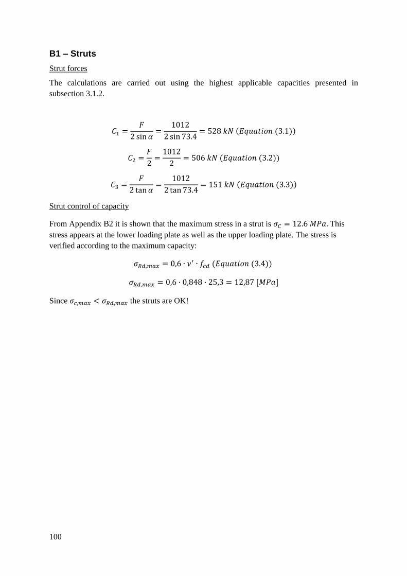
100
B1 – Struts
Strut forces
The calculations are carried out using the highest applicable capacities presented in
subsection 3.1.2.
𝐶1 =𝐹
2 sin 𝛼=
1012
2 sin 73.4= 528 𝑘𝑁 (𝐸𝑞𝑢𝑎𝑡𝑖𝑜𝑛 (3.1))
𝐶2 =𝐹
2=
1012
2= 506 𝑘𝑁 (𝐸𝑞𝑢𝑎𝑡𝑖𝑜𝑛 (3.2))
𝐶3 =𝐹
2 tan 𝛼=
1012
2 tan 73.4= 151 𝑘𝑁 (𝐸𝑞𝑢𝑎𝑡𝑖𝑜𝑛 (3.3))
Strut control of capacity
From Appendix B2 it is shown that the maximum stress in a strut is 𝜎𝐶 = 12.6 𝑀𝑃𝑎. This
stress appears at the lower loading plate as well as the upper loading plate. The stress is
verified according to the maximum capacity:
𝜎𝑅𝑑,𝑚𝑎𝑥 = 0,6 ∙ 𝜈′ ∙ 𝑓𝑐𝑑 (𝐸𝑞𝑢𝑎𝑡𝑖𝑜𝑛 (3.4))
𝜎𝑅𝑑,𝑚𝑎𝑥 = 0,6 · 0,848 · 25,3 = 12,87 [𝑀𝑃𝑎]
Since 𝜎𝑐,𝑚𝑎𝑥 < 𝜎𝑅𝑑,𝑚𝑎𝑥 the struts are OK!
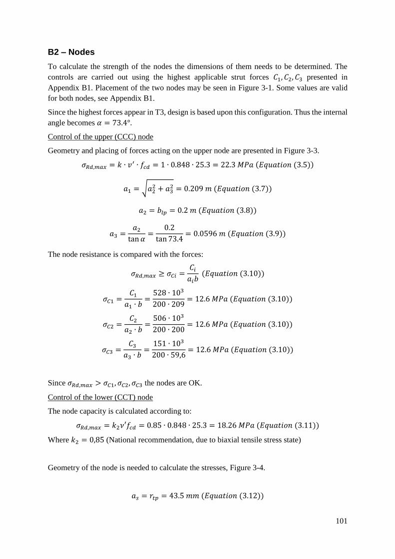
101
B2 – Nodes
To calculate the strength of the nodes the dimensions of them needs to be determined. The
controls are carried out using the highest applicable strut forces 𝐶1, 𝐶2, 𝐶3 presented in
Appendix B1. Placement of the two nodes may be seen in Figure 3-1. Some values are valid
for both nodes, see Appendix B1.
Since the highest forces appear in T3, design is based upon this configuration. Thus the internal
angle becomes 𝛼 = 73.4°.
Control of the upper (CCC) node
Geometry and placing of forces acting on the upper node are presented in Figure 3-3.
𝜎𝑅𝑑,𝑚𝑎𝑥 = 𝑘 ∙ 𝑣′ ∙ 𝑓𝑐𝑑 = 1 ∙ 0.848 ∙ 25.3 = 22.3 𝑀𝑃𝑎 (𝐸𝑞𝑢𝑎𝑡𝑖𝑜𝑛 (3.5))
𝑎1 = √𝑎22 + 𝑎3
2 = 0.209 𝑚 (𝐸𝑞𝑢𝑎𝑡𝑖𝑜𝑛 (3.7))
𝑎2 = 𝑏𝑙𝑝 = 0.2 𝑚 (𝐸𝑞𝑢𝑎𝑡𝑖𝑜𝑛 (3.8))
𝑎3 =𝑎2
tan 𝛼=
0.2
tan 73.4= 0.0596 𝑚 (𝐸𝑞𝑢𝑎𝑡𝑖𝑜𝑛 (3.9))
The node resistance is compared with the forces:
𝜎𝑅𝑑,𝑚𝑎𝑥 ≥ 𝜎𝐶𝑖 =𝐶𝑖
𝑎𝑖𝑏 (𝐸𝑞𝑢𝑎𝑡𝑖𝑜𝑛 (3.10))
𝜎𝐶1 =𝐶1
𝑎1 ∙ 𝑏=
528 ∙ 103
200 ∙ 209= 12.6 𝑀𝑃𝑎 (𝐸𝑞𝑢𝑎𝑡𝑖𝑜𝑛 (3.10))
𝜎𝐶2 =𝐶2
𝑎2 ∙ 𝑏=
506 ∙ 103
200 ∙ 200= 12.6 𝑀𝑃𝑎 (𝐸𝑞𝑢𝑎𝑡𝑖𝑜𝑛 (3.10))
𝜎𝐶3 =𝐶3
𝑎3 ∙ 𝑏=
151 ∙ 103
200 ∙ 59,6= 12.6 𝑀𝑃𝑎 (𝐸𝑞𝑢𝑎𝑡𝑖𝑜𝑛 (3.10))
Since 𝜎𝑅𝑑,𝑚𝑎𝑥 > 𝜎𝐶1, 𝜎𝐶2, 𝜎𝐶3 the nodes are OK.
Control of the lower (CCT) node
The node capacity is calculated according to:
𝜎𝑅𝑑,𝑚𝑎𝑥 = 𝑘2𝜈′𝑓𝑐𝑑 = 0.85 ∙ 0.848 ∙ 25.3 = 18.26 𝑀𝑃𝑎 (𝐸𝑞𝑢𝑎𝑡𝑖𝑜𝑛 (3.11))
Where 𝑘2 = 0,85 (National recommendation, due to biaxial tensile stress state)
Geometry of the node is needed to calculate the stresses, Figure 3-4.
𝑎𝑠 = 𝑟𝑡𝑝 = 43.5 𝑚𝑚 (𝐸𝑞𝑢𝑎𝑡𝑖𝑜𝑛 (3.12))
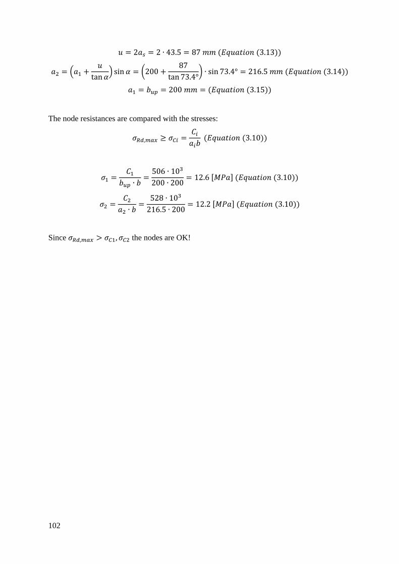
102
𝑢 = 2𝑎𝑠 = 2 ∙ 43.5 = 87 𝑚𝑚 (𝐸𝑞𝑢𝑎𝑡𝑖𝑜𝑛 (3.13))
𝑎2 = (𝑎1 +𝑢
tan 𝛼) sin 𝛼 = (200 +
87
tan 73.4°) ∙ sin 73.4° = 216.5 𝑚𝑚 (𝐸𝑞𝑢𝑎𝑡𝑖𝑜𝑛 (3.14))
𝑎1 = 𝑏𝑢𝑝 = 200 𝑚𝑚 = (𝐸𝑞𝑢𝑎𝑡𝑖𝑜𝑛 (3.15))
The node resistances are compared with the stresses:
𝜎𝑅𝑑,𝑚𝑎𝑥 ≥ 𝜎𝐶𝑖 =𝐶𝑖
𝑎𝑖𝑏 (𝐸𝑞𝑢𝑎𝑡𝑖𝑜𝑛 (3.10))
𝜎1 =𝐶1
𝑏𝑢𝑝 ∙ 𝑏=
506 ∙ 103
200 ∙ 200= 12.6 [𝑀𝑃𝑎] (𝐸𝑞𝑢𝑎𝑡𝑖𝑜𝑛 (3.10))
𝜎2 =𝐶2
𝑎2 ∙ 𝑏=
528 ∙ 103
216.5 ∙ 200= 12.2 [𝑀𝑃𝑎] (𝐸𝑞𝑢𝑎𝑡𝑖𝑜𝑛 (3.10))
Since 𝜎𝑅𝑑,𝑚𝑎𝑥 > 𝜎𝐶1, 𝜎𝐶2 the nodes are OK!
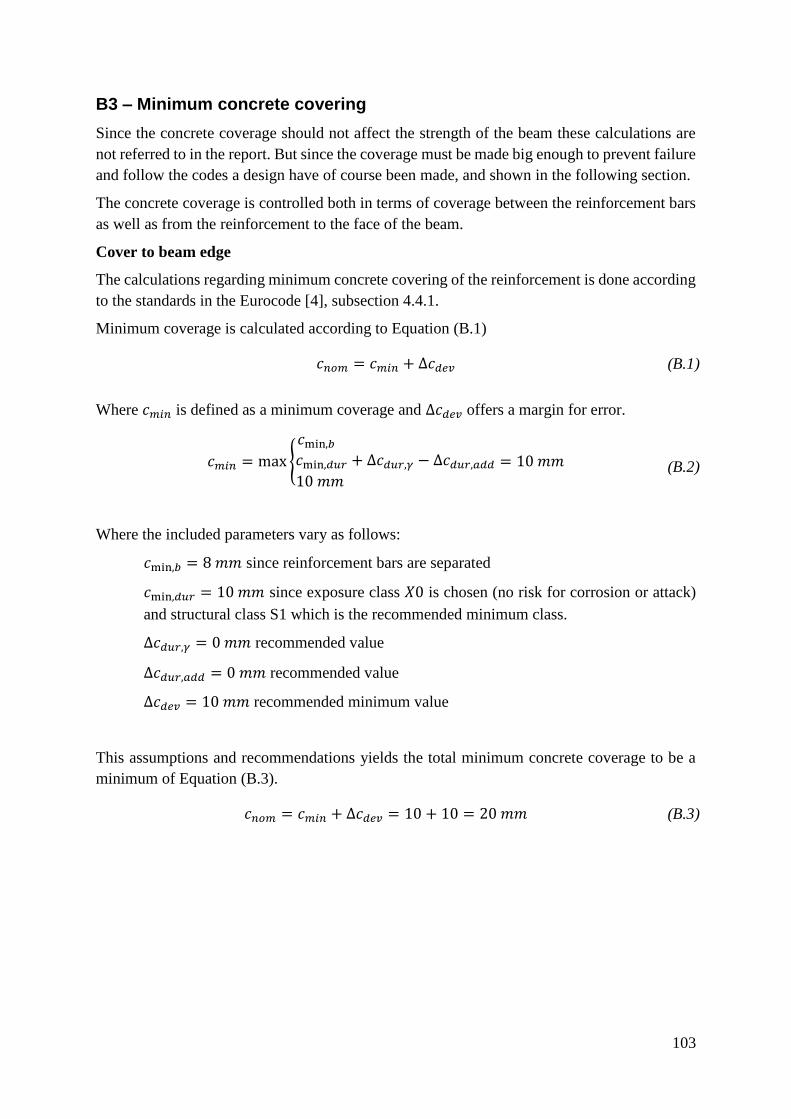
103
B3 – Minimum concrete covering
Since the concrete coverage should not affect the strength of the beam these calculations are
not referred to in the report. But since the coverage must be made big enough to prevent failure
and follow the codes a design have of course been made, and shown in the following section.
The concrete coverage is controlled both in terms of coverage between the reinforcement bars
as well as from the reinforcement to the face of the beam.
Cover to beam edge
The calculations regarding minimum concrete covering of the reinforcement is done according
to the standards in the Eurocode [4], subsection 4.4.1.
Minimum coverage is calculated according to Equation (B.1)
𝑐𝑛𝑜𝑚 = 𝑐𝑚𝑖𝑛 + Δ𝑐𝑑𝑒𝑣 (B.1)
Where 𝑐𝑚𝑖𝑛 is defined as a minimum coverage and Δ𝑐𝑑𝑒𝑣 offers a margin for error.
𝑐𝑚𝑖𝑛 = max {
𝑐min,𝑏
𝑐min,𝑑𝑢𝑟 + Δ𝑐𝑑𝑢𝑟,𝛾 − Δ𝑐𝑑𝑢𝑟,𝑎𝑑𝑑
10 𝑚𝑚
= 10 𝑚𝑚
(B.2)
Where the included parameters vary as follows:
𝑐min,𝑏 = 8 𝑚𝑚 since reinforcement bars are separated
𝑐min,𝑑𝑢𝑟 = 10 𝑚𝑚 since exposure class 𝑋0 is chosen (no risk for corrosion or attack)
and structural class S1 which is the recommended minimum class.
Δ𝑐𝑑𝑢𝑟,𝛾 = 0 𝑚𝑚 recommended value
Δ𝑐𝑑𝑢𝑟,𝑎𝑑𝑑 = 0 𝑚𝑚 recommended value
Δ𝑐𝑑𝑒𝑣 = 10 𝑚𝑚 recommended minimum value
This assumptions and recommendations yields the total minimum concrete coverage to be a
minimum of Equation (B.3).
𝑐𝑛𝑜𝑚 = 𝑐𝑚𝑖𝑛 + Δ𝑐𝑑𝑒𝑣 = 10 + 10 = 20 𝑚𝑚 (B.3)
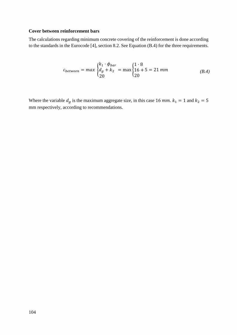
104
Cover between reinforcement bars
The calculations regarding minimum concrete covering of the reinforcement is done according
to the standards in the Eurocode [4], section 8.2. See Equation (B.4) for the three requirements.
𝑐𝑏𝑒𝑡𝑤𝑒𝑒𝑛 = 𝑚𝑎𝑥 {𝑘1 · 𝜙𝑏𝑎𝑟
𝑑𝑔 + 𝑘2
20
= max {1 · 8 16 +20
5 = 21 𝑚𝑚
(B.4)
Where the variable 𝑑𝑔 is the maximum aggregate size, in this case 16 𝑚𝑚. 𝑘1 = 1 and 𝑘2 = 5
mm respectively, according to recommendations.
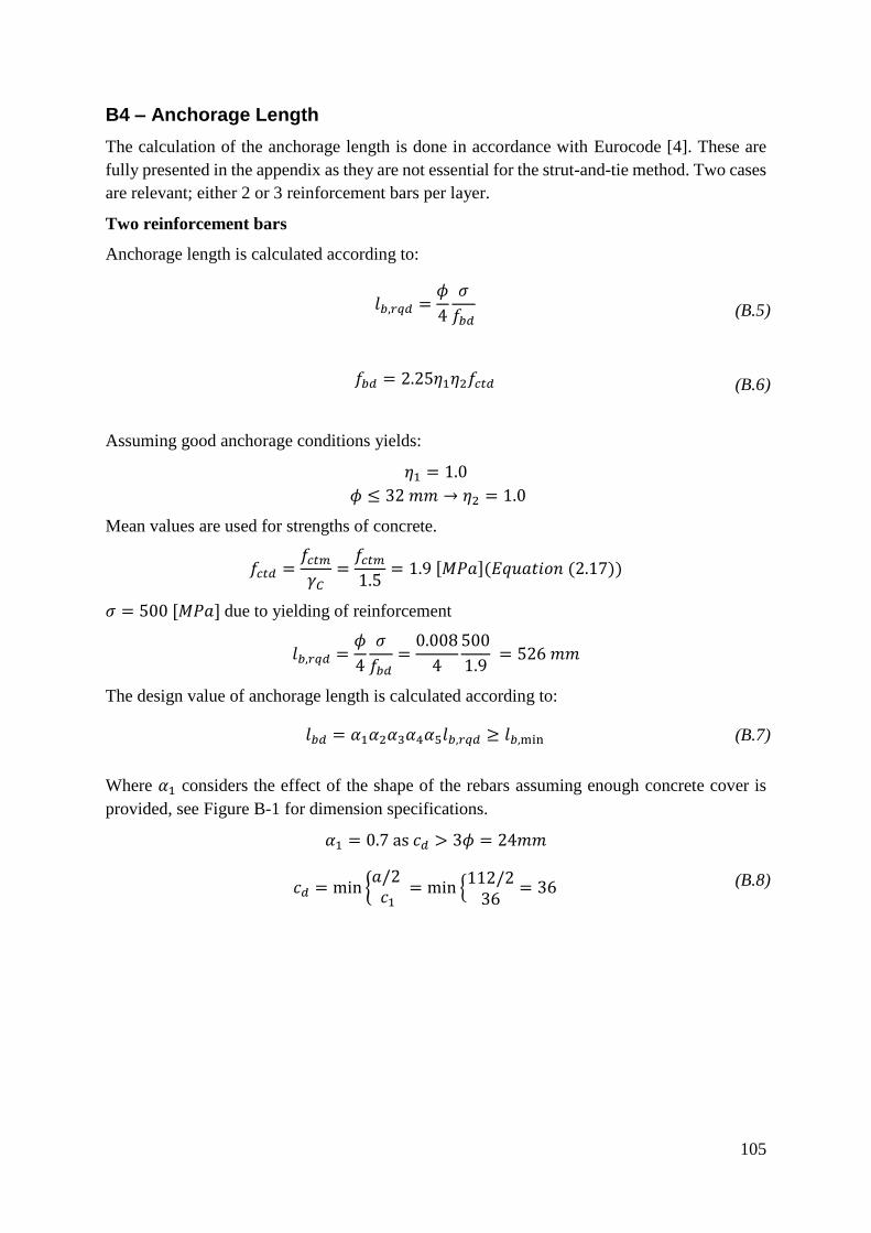
105
B4 – Anchorage Length
The calculation of the anchorage length is done in accordance with Eurocode [4]. These are
fully presented in the appendix as they are not essential for the strut-and-tie method. Two cases
are relevant; either 2 or 3 reinforcement bars per layer.
Two reinforcement bars
Anchorage length is calculated according to:
𝑙𝑏,𝑟𝑞𝑑 =
𝜙
4
𝜎
𝑓𝑏𝑑
(B.5)
𝑓𝑏𝑑 = 2.25𝜂1𝜂2𝑓𝑐𝑡𝑑
(B.6)
Assuming good anchorage conditions yields:
𝜂1 = 1.0
𝜙 ≤ 32 𝑚𝑚 → 𝜂2 = 1.0
Mean values are used for strengths of concrete.
𝑓𝑐𝑡𝑑 =𝑓𝑐𝑡𝑚
𝛾𝐶=
𝑓𝑐𝑡𝑚
1.5= 1.9 [𝑀𝑃𝑎](𝐸𝑞𝑢𝑎𝑡𝑖𝑜𝑛 (2.17))
𝜎 = 500 [𝑀𝑃𝑎] due to yielding of reinforcement
𝑙𝑏,𝑟𝑞𝑑 =𝜙
4
𝜎
𝑓𝑏𝑑=
0.008
4
500
1.9 = 526 𝑚𝑚
The design value of anchorage length is calculated according to:
𝑙𝑏𝑑 = 𝛼1𝛼2𝛼3𝛼4𝛼5𝑙𝑏,𝑟𝑞𝑑 ≥ 𝑙𝑏,min (B.7)
Where 𝛼1 considers the effect of the shape of the rebars assuming enough concrete cover is
provided, see Figure B-1 for dimension specifications.
𝛼1 = 0.7 as 𝑐𝑑 > 3𝜙 = 24𝑚𝑚
𝑐𝑑 = min {
𝑎/2 𝑐1
= min {112/2
36= 36 (B.8)
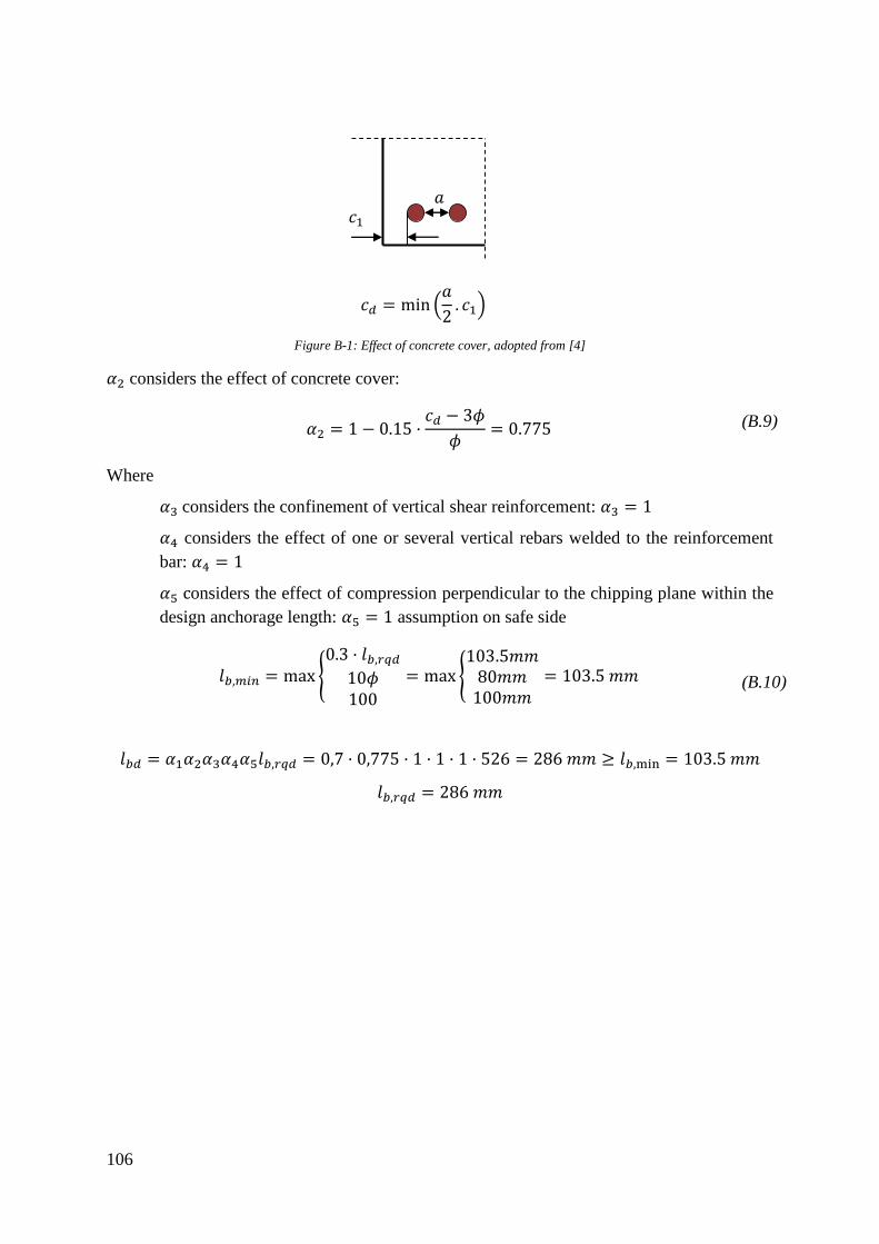
106
Figure B-1: Effect of concrete cover, adopted from [4]
𝛼2 considers the effect of concrete cover:
𝛼2 = 1 − 0.15 ·
𝑐𝑑 − 3𝜙
𝜙= 0.775 (B.9)
Where
𝛼3 considers the confinement of vertical shear reinforcement: 𝛼3 = 1
𝛼4 considers the effect of one or several vertical rebars welded to the reinforcement
bar: 𝛼4 = 1
𝛼5 considers the effect of compression perpendicular to the chipping plane within the
design anchorage length: 𝛼5 = 1 assumption on safe side
𝑙𝑏,𝑚𝑖𝑛 = max {0.3 · 𝑙𝑏,𝑟𝑞𝑑
10𝜙100
= max {103.5𝑚𝑚
80𝑚𝑚100𝑚𝑚
= 103.5 𝑚𝑚
(B.10)
𝑙𝑏𝑑 = 𝛼1𝛼2𝛼3𝛼4𝛼5𝑙𝑏,𝑟𝑞𝑑 = 0,7 · 0,775 · 1 · 1 · 1 · 526 = 286 𝑚𝑚 ≥ 𝑙𝑏,min = 103.5 𝑚𝑚
𝑙𝑏,𝑟𝑞𝑑 = 286 𝑚𝑚
𝑎 𝑐1
𝑐𝑑 = min (𝑎
2. 𝑐1)
107
Three reinforcement bars
Anchorage length is calculated according to Equation (B.5) and (B.6).
Assuming good anchorage conditions yields:
𝜂1 = 1.0
𝜙 ≤ 32 𝑚𝑚 → 𝜂2 = 1.0
Mean values are used for strengths of concrete.
𝑓𝑐𝑡𝑑 = 1.9 [𝑀𝑃𝑎] (𝐸𝑞𝑢𝑎𝑡𝑖𝑜𝑛 (2.17))
𝜎 = 500 [𝑀𝑃𝑎] due to assumed yielding of reinforcement
𝑙𝑏,𝑟𝑞𝑑 =𝜙
4
𝜎
𝑓𝑏𝑑=
0.008
4
500
1.9 = 526 𝑚𝑚
The design value of anchorage length is calculated according to:
𝑙𝑏𝑑 = 𝛼1𝛼2𝛼3𝛼4𝛼5𝑙𝑏,𝑟𝑞𝑑 ≥ 𝑙𝑏,min
Where 𝛼1 considers the effect of the shape of the rebars assuming enough concrete cover is
provided
𝛼1 = 0.7 as 𝑐𝑑 > 3𝜙 = 24𝑚𝑚
𝑐𝑑 = min {𝑎/2
𝑐1= min {
1122 −
82
236
= 26 𝑚𝑚
𝛼2 considers the effect of concrete cover:
𝛼2 = 1 − 0.15 ·𝑐𝑑 − 3𝜙
𝜙= 0.9625
𝛼3 considers the confinement of vertical shear reinforcement: 𝛼3 = 1
𝛼4 considers the effect of one or several vertical rebars welded to the reinforcement bar: 𝛼4 =
1
𝛼5 considers the effect of compression perpendicular to the chipping plane within the design
anchorage length: 𝛼5 = 1 assumption on safe side
𝑙𝑏,𝑚𝑖𝑛 = max {0.3 · 𝑙𝑏,𝑟𝑞𝑑
10𝜙100
= max {103.5𝑚𝑚
80𝑚𝑚100𝑚𝑚
= 103.5 𝑚𝑚
𝑙𝑏𝑑 = 𝛼1𝛼2𝛼3𝛼4𝛼5𝑙𝑏,𝑟𝑞𝑑 = 0.7 · 0.9625 · 1 · 1 · 1 · 526 = 354 𝑚𝑚 ≥ 𝑙𝑏,min = 103.5 𝑚𝑚
𝑙𝑏,𝑟𝑞𝑑 = 354 𝑚𝑚
108
B5– Load Bearing Capacity
The load bearing capacity of the beams are calculated in accordance with chapter 3. The
calculations are divided into specimens T1, T2, T3 and T4. The load placement is shown in
Figure 1-1 and the equilibrium is shown in Figure 3-5. Calculations are made for angles of
𝛼 = 73.4° 𝑜𝑟 73.6°, 𝛼 = 60° and 𝛼 = 45° for all specimens. All calculations are based on
Equation (3.21).
T1
𝐴𝑠 = 2 · 𝜙8
𝛼 = 73,6 °
𝐹 = 2 ∙ 500 ∙ 2 ∙0.0082 ∙ 𝜋
4∙ tan 73,6 = 342 𝑘𝑁
𝛼 = 60 °
𝐹 = 2 ∙ 500 ∙ 2 ∙0.0082 ∙ 𝜋
4∙ tan 60 = 201 𝑘𝑁
𝛼 = 45 °
𝐹 = 2 ∙ 500 ∙ 2 ∙0.0082 ∙ 𝜋
4∙ tan 45 = 174 𝑘𝑁
T2
𝐴𝑠 = 4 · 𝜙8
𝛼 = 73,4 °
𝐹 = 2 ∙ 500 ∙ 4 ∙0.0082 ∙ 𝜋
4∙ tan 73,4 = 674 𝑘𝑁
𝛼 = 60 °
𝐹 = 2 ∙ 500 ∙ 4 ∙0.0082 ∙ 𝜋
4∙ tan 60 = 348 𝑘𝑁
𝛼 = 45 °
𝐹 = 2 ∙ 500 ∙ 4 ∙0.0082 ∙ 𝜋
4∙ tan 45 = 201 𝑘𝑁
T3
𝐴𝑠 = 6 · 𝜙8
𝛼 = 73,4 °
𝐹 = 2 ∙ 500 ∙ 6 ∙0.0082 ∙ 𝜋
4∙ tan 73,4 = 1012 𝑘𝑁
𝛼 = 60 °
𝐹 = 2 ∙ 500 ∙ 6 ∙0.0082 ∙ 𝜋
4∙ tan 60 = 522 𝑘𝑁
109
𝛼 = 45 °
𝐹 = 2 ∙ 500 ∙ 6 ∙0.0082 ∙ 𝜋
4∙ tan 45 = 302 𝑘𝑁
T4
As T4 has the same primary reinforcement as T2, and the minimum-reinforcement is assumed
not to provide any additional strength, this specimen is assumed to withstand the same load as
T2.

110
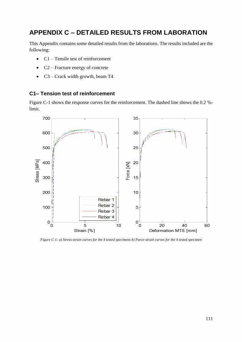
111
APPENDIX C – DETAILED RESULTS FROM LABORATION
This Appendix contains some detailed results from the laborations. The results included are the
following:
C1 – Tensile test of reinforcement
C2 – Fracture energy of concrete
C3 – Crack width growth, beam T4
C1– Tension test of reinforcement
Figure C-1 shows the response curves for the reinforcement. The dashed line shows the 0.2 %-
limit.
Figure C-1: a) Stress-strain curves for the 4 tested specimens b) Force-strain curves for the 4 tested specimen
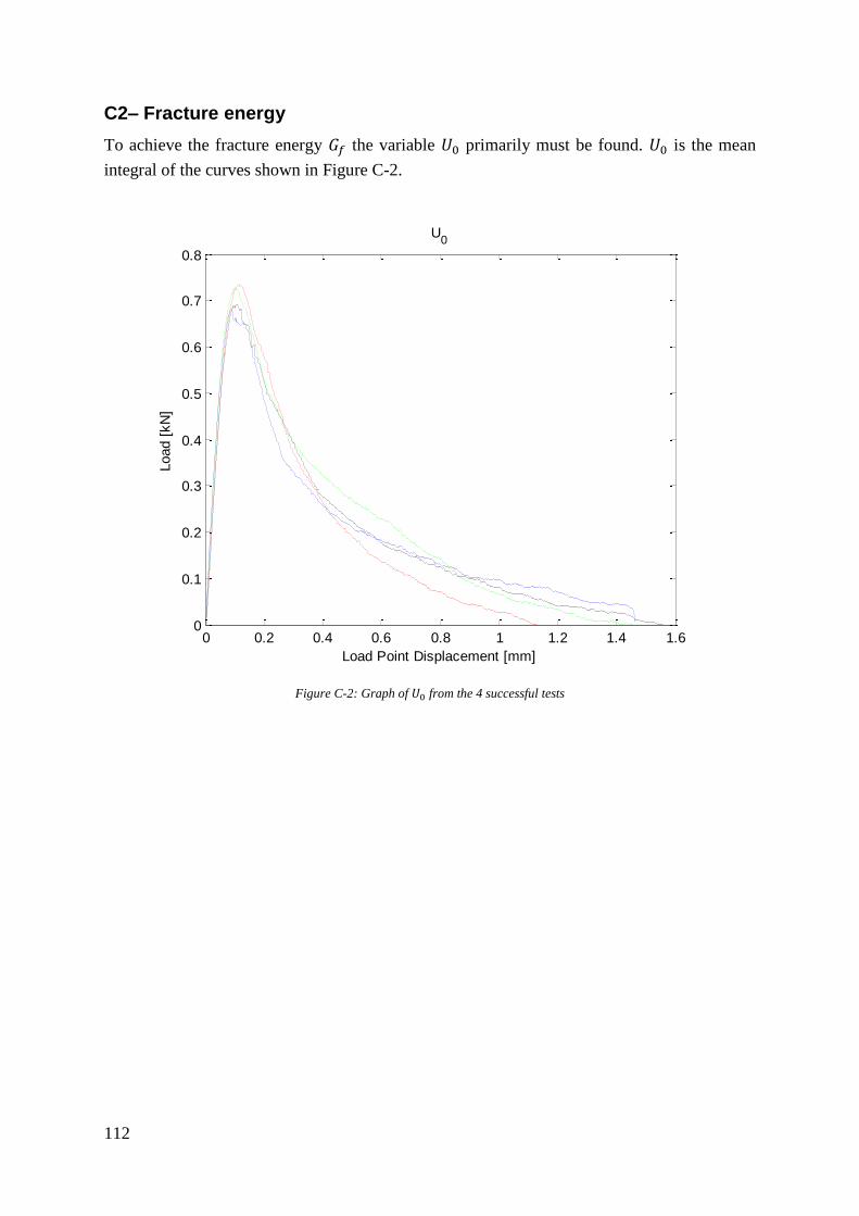
112
C2– Fracture energy
To achieve the fracture energy 𝐺𝑓 the variable 𝑈0 primarily must be found. 𝑈0 is the mean
integral of the curves shown in Figure C-2.
Figure C-2: Graph of 𝑈0 from the 4 successful tests
0 0.2 0.4 0.6 0.8 1 1.2 1.4 1.60
0.1
0.2
0.3
0.4
0.5
0.6
0.7
0.8
U0
Load Point Displacement [mm]
Load [
kN
]
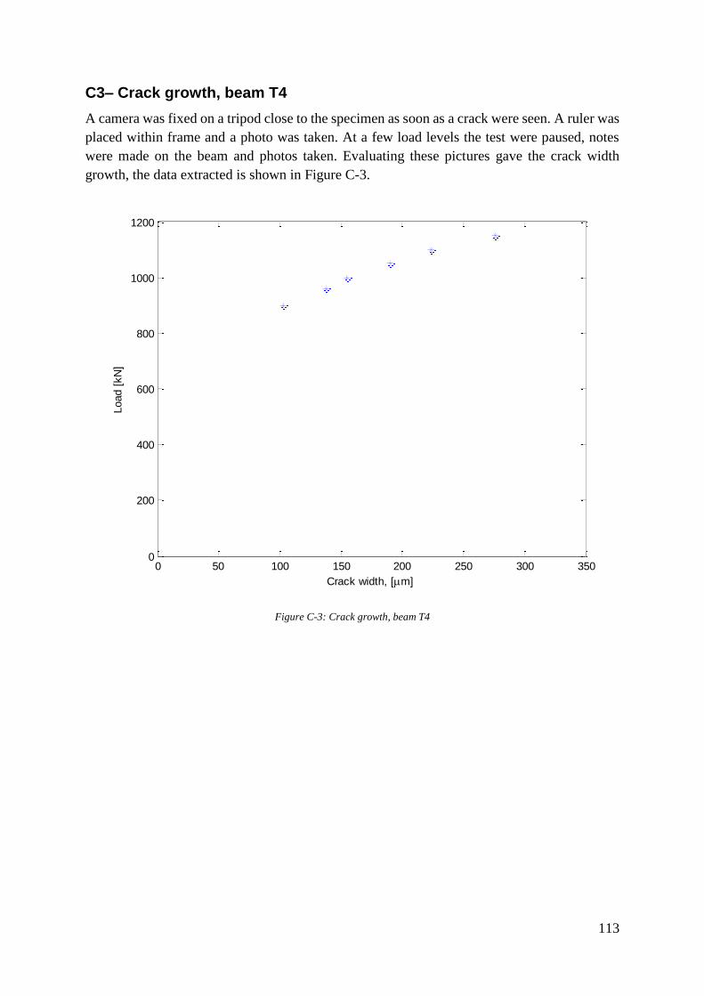
113
C3– Crack growth, beam T4
A camera was fixed on a tripod close to the specimen as soon as a crack were seen. A ruler was
placed within frame and a photo was taken. At a few load levels the test were paused, notes
were made on the beam and photos taken. Evaluating these pictures gave the crack width
growth, the data extracted is shown in Figure C-3.
Figure C-3: Crack growth, beam T4
0 50 100 150 200 250 300 3500
200
400
600
800
1000
1200
Crack width, [m]
Load [
kN
]

114
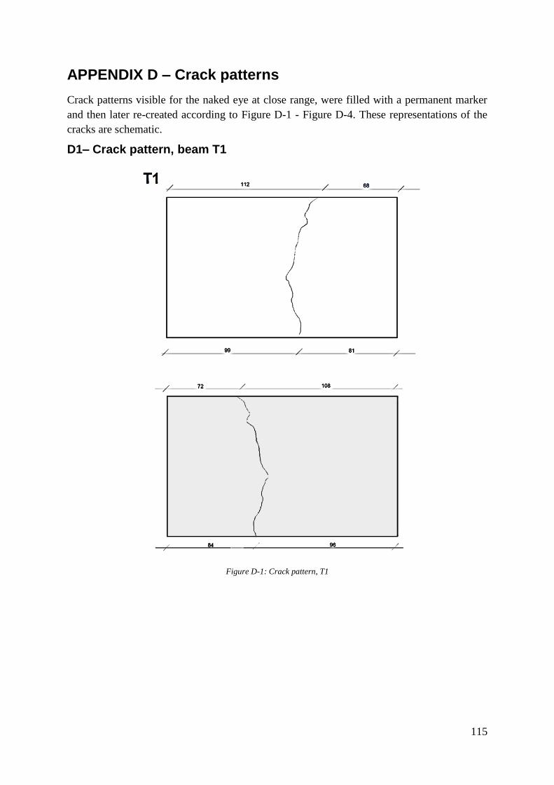
115
APPENDIX D – Crack patterns
Crack patterns visible for the naked eye at close range, were filled with a permanent marker
and then later re-created according to Figure D-1 - Figure D-4. These representations of the
cracks are schematic.
D1– Crack pattern, beam T1
Figure D-1: Crack pattern, T1
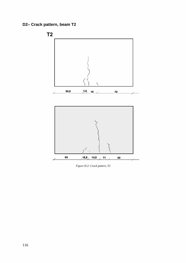
116
D2– Crack pattern, beam T2
Figure D-2: Crack pattern, T2
117
D3– Crack pattern, beam T3
Figure D-3: Crack pattern, T3
118
D4– Crack pattern, beam T4
Figure D-4: Crack pattern, T4