Embed Size (px)
Citation preview

Limited Feedback Information in WirelessCommunications: Transmission Schemes and
Performance Bounds
TÙNG T. KIM
Doctoral Thesis in TelecommunicationsStockholm, Sweden 2008

TRITA-EE 2008:022ISSN 1653-5146ISBN 978-91-7178-950-1
KTH School of Electrical EngineeringSE-100 44 Stockholm
SWEDEN
Akademisk avhandling som med tillstånd av Kungl Tekniska högskolan framläggestill offentlig granskning för avläggande av teknologie doktorsexamen i telekommu-nikation fredagen den 30 maj 2008 klockan 14.00 i Hörsal D3, Lindstedtsvägen 5,Stockholm.
© Tùng T. Kim, May 2008
Tryck: Universitetsservice US AB

iii
Abstract
This thesis studies some fundamental aspects of wireless systems withpartial channel state information at the transmitter (CSIT), with a specialemphasis on the high signal-to-noise ratio (SNR) regime. The first contri-bution is a study on multi-layer variable-rate communication systems withquantized feedback, where the expected rate is chosen as the performancemeasure. Iterative algorithms exploiting results in the literature of parallelbroadcast channels are developed to design the system parameters. Necessaryand sufficient conditions for single-layer coding to be optimal are derived. Incontrast to the ergodic case, it is shown that a few bits of feedback informationcan improve the expected rate dramatically.
The next part of the thesis is devoted to characterizing the tradeoff be-tween diversity and multiplexing gains (D–M tradeoff) over slow fading chan-nels with partial CSIT. In the multiple-input multiple-output (MIMO) case,we introduce the concept of minimum guaranteed multiplexing gain in theforward link and show that it influences the D–M tradeoff significantly. Itis demonstrated that power control based on the feedback is instrumental inachieving the D-M tradeoff, and that rate adaptation is important in obtain-ing a high diversity gain even at high rates.
Extending the D–M tradeoff analysis to decode-and-forward relay chan-nels with quantized channel state feedback, we consider several different sce-narios. In the relay-to-source feedback case, it is found that using just onebit of feedback to control the source transmit power is sufficient to achievethe multiantenna upper bound in a range of multiplexing gains. In thedestination-to-source-and-relay feedback scenario, if the source-relay channelgain is unknown to the feedback quantizer at the destination, the diversitygain only grows linearly in the number of feedback levels, in sharp contrastto an exponential growth for MIMO channels.
We also consider the achievable D–M tradeoff of a relay network with thecompress-and-forward protocol when the relay is constrained to make use ofstandard source coding. Under a short-term power constraint at the relay,using source coding without side information results in a significant loss interms of the D–M tradeoff. For a range of multiplexing gains, this loss canbe fully compensated for by using power control at the relay.
The final part of the thesis deals with the transmission of an analog Gaus-sian source over quasi-static fading channels with limited CSIT, taking theSNR exponent of the end-to-end average distortion as performance measure.Building upon results from the D–M tradeoff analysis, we develop novel up-perbounds on the distortion exponents achieved with partial CSIT. We showthat in order to achieve the optimal scaling, the CSIT feedback resolutionmust grow logarithmically with the bandwidth ratio for MIMO channels. Theachievable distortion exponent of some hybrid schemes with heavily quantizedfeedback is also derived. As for the half-duplex fading relay channel, com-bining a simple feedback scheme with separate source and channel codingoutperforms the best known no-feedback strategies even with only a few bitsof feedback information.


Acknowledgement
I would like to express my gratitude to Professor Mikael Skoglund, who has takengreat effort to walk me into the world of science, and beyond (as evident from ourlong drive to Death Valley). I am grateful that Mikael has given me an incredibleopportunity to pursue my research, and that he has provided invaluable guidanceand limitless support during my wonderful time at KTH.
I would also like to thank Professor Giuseppe Caire for hosting me with hisgroup at University of Southern California. Despite his incredibly busy schedule,Giuseppe has managed to spend a large amount of time helping me attack researchproblems of common interest.
It has been a great pleasure to work alongside my colleagues in the Communi-cation Theory and Signal Processing groups. Especially, I would like to thank Dr.George Jöngren for introducing me to the field of limited feedback, Dr. JoakimJaldén for posing thoughtful questions that inspired deeper studies on some prob-lems in this thesis, and Lei Bao, for going out of her way to help me on countlessoccasions. Thanks to the excellent administrative personnel, among them are An-nika Augustsson and Karin Demin, and to the computer support team, the workingenvironment at KTH has been running so smoothly that I could totally focus onmy work. I also thank my fellow students at USC, especially Ozgun Bursaliogluand Raj Kumar, for making my stay in Los Angeles a pleasant one.
I have greatly enjoyed working with my co-authors, who have given me theluxury of leaving out a couple of journal papers from the thesis. In particular,Professor Mats Bengtsson and Professor Erik G. Larsson’s contribution has beenextremely helpful, for which I am grateful.
Thanks are due to Professor Hesham El Gamal from Ohio State University foracting as opponent for the thesis. I also thank the committee members: Profes-sor Eduard Jorswieck from TU Dresden, Professor Ulf Jönsson from KTH, andProfessor Ralf Müller from NTNU.
Last but definitely not least, I feel deeply indebted to my family for their ab-solute support and patience during my seemingly endless academic training. Iespecially thank my wife Hải Yến for quietly nourishing love and keeping happinessunder our small roof.
v

Contents
Contents vi
1 Introduction 11.1 Communication Systems . . . . . . . . . . . . . . . . . . . . . . . . . 21.2 Fading Channels . . . . . . . . . . . . . . . . . . . . . . . . . . . . . 31.3 Slow Fading . . . . . . . . . . . . . . . . . . . . . . . . . . . . . . . . 41.4 Channel-state Information . . . . . . . . . . . . . . . . . . . . . . . . 51.5 Some Information-theoretic Performance Measures on Fading Channels 61.6 Multiple-antenna Systems . . . . . . . . . . . . . . . . . . . . . . . . 91.7 Diversity–Multiplexing Tradeoff . . . . . . . . . . . . . . . . . . . . . 111.8 Distortion Exponent . . . . . . . . . . . . . . . . . . . . . . . . . . . 131.9 Contributions and Outline . . . . . . . . . . . . . . . . . . . . . . . . 141.10 Notation and Acronyms . . . . . . . . . . . . . . . . . . . . . . . . . 19
I Expected Rate 21
2 Expected Rate Maximization 232.1 Introduction . . . . . . . . . . . . . . . . . . . . . . . . . . . . . . . . 232.2 System Model . . . . . . . . . . . . . . . . . . . . . . . . . . . . . . . 252.3 Single-layer Coding . . . . . . . . . . . . . . . . . . . . . . . . . . . . 272.4 Multiple-layer Coding . . . . . . . . . . . . . . . . . . . . . . . . . . 322.5 Numerical Results . . . . . . . . . . . . . . . . . . . . . . . . . . . . 362.6 Conclusion . . . . . . . . . . . . . . . . . . . . . . . . . . . . . . . . 392.A Proof of Proposition 2.1 . . . . . . . . . . . . . . . . . . . . . . . . . 41
II Diversity–Multiplexing Tradeoff 45
3 D–M Tradeoff in MIMO Channels 473.1 Introduction . . . . . . . . . . . . . . . . . . . . . . . . . . . . . . . . 473.2 System Model . . . . . . . . . . . . . . . . . . . . . . . . . . . . . . . 493.3 Outage Upper Bound on the Optimal D–M Tradeoff . . . . . . . . . 52
vi

Contents vii
3.4 Achievability of the Optimal D–M Tradeoff . . . . . . . . . . . . . . 573.5 Lower Bounds on the Optimal D–M Tradeoff: Gaussian Coding Bounds 683.6 Conclusion . . . . . . . . . . . . . . . . . . . . . . . . . . . . . . . . 773.A Proof of Lemma 3.1 . . . . . . . . . . . . . . . . . . . . . . . . . . . 783.B Proof of Theorem 3.1 . . . . . . . . . . . . . . . . . . . . . . . . . . . 793.C Proof of Theorem 3.2 . . . . . . . . . . . . . . . . . . . . . . . . . . . 803.D Towards the Necessity of (3.18) . . . . . . . . . . . . . . . . . . . . . 82
4 D–M Tradeoff in Decode–and–Forward Relay Channels 854.1 Introduction . . . . . . . . . . . . . . . . . . . . . . . . . . . . . . . . 854.2 System Model . . . . . . . . . . . . . . . . . . . . . . . . . . . . . . . 874.3 Decode-and-Forward without CSF . . . . . . . . . . . . . . . . . . . 894.4 Relay-to-Source CSF . . . . . . . . . . . . . . . . . . . . . . . . . . . 924.5 Destination-to-Relay CSF . . . . . . . . . . . . . . . . . . . . . . . . 994.6 Destination-to-Source-and-Relay CSF . . . . . . . . . . . . . . . . . 1044.7 On Finite-length Codes . . . . . . . . . . . . . . . . . . . . . . . . . 1084.8 Conclusion . . . . . . . . . . . . . . . . . . . . . . . . . . . . . . . . 1144.A Proof of Proposition 4.2 . . . . . . . . . . . . . . . . . . . . . . . . . 1154.B Proof of Proposition 4.3 . . . . . . . . . . . . . . . . . . . . . . . . . 1164.C Proof of Proposition 4.4 . . . . . . . . . . . . . . . . . . . . . . . . . 1184.D Proof of Proposition 4.5 . . . . . . . . . . . . . . . . . . . . . . . . . 1204.E Destination-Relay CSF . . . . . . . . . . . . . . . . . . . . . . . . . . 1224.F Proof of Proposition 4.8 . . . . . . . . . . . . . . . . . . . . . . . . . 1254.G Proof of Proposition 4.10 . . . . . . . . . . . . . . . . . . . . . . . . 126
5 D–M Tradeoff in Compress–and–Forward Relay Channels 1295.1 Introduction . . . . . . . . . . . . . . . . . . . . . . . . . . . . . . . . 1295.2 System Model . . . . . . . . . . . . . . . . . . . . . . . . . . . . . . . 1305.3 Proof of Proposition 5.1 . . . . . . . . . . . . . . . . . . . . . . . . . 1365.4 Proof of Proposition 5.2 . . . . . . . . . . . . . . . . . . . . . . . . . 140
III End-to-end Distortion Exponent 143
6 Distortion Exponent over MIMO Channels 1456.1 Introduction . . . . . . . . . . . . . . . . . . . . . . . . . . . . . . . . 1456.2 System Model . . . . . . . . . . . . . . . . . . . . . . . . . . . . . . . 1486.3 Upper Bounds on Partial-CSIT Distortion Exponent . . . . . . . . . 1496.4 Achievable Distortion Exponents: HDA with Dimension Splitting . . 1576.5 Achievable Distortion Exponents: HDA with Power Splitting . . . . 1606.6 Numerical Examples . . . . . . . . . . . . . . . . . . . . . . . . . . . 1646.7 Conclusion . . . . . . . . . . . . . . . . . . . . . . . . . . . . . . . . 1666.A Partial-CSIT Upper Bound . . . . . . . . . . . . . . . . . . . . . . . 167

viii Contents
6.B Derivation of K-level Upper Bound and Achievable Distortion Ex-ponent for SISO Channels . . . . . . . . . . . . . . . . . . . . . . . . 172
6.C Proof of Proposition 6.3 . . . . . . . . . . . . . . . . . . . . . . . . . 1746.D Proof of Proposition 6.4 . . . . . . . . . . . . . . . . . . . . . . . . . 1776.E Proof of Proposition 6.5 . . . . . . . . . . . . . . . . . . . . . . . . . 1806.F Proof of Proposition 6.6 . . . . . . . . . . . . . . . . . . . . . . . . . 181
7 Distortion Exponent over Relay Channels 1837.1 Introduction . . . . . . . . . . . . . . . . . . . . . . . . . . . . . . . . 1837.2 System Model . . . . . . . . . . . . . . . . . . . . . . . . . . . . . . . 1857.3 Distortion Exponents with Channel State Feedback . . . . . . . . . . 1857.4 Distortion Exponents with a Restricted Feedback Quantizer . . . . . 1957.5 Conclusion . . . . . . . . . . . . . . . . . . . . . . . . . . . . . . . . 1987.A Proof of Proposition 7.1 . . . . . . . . . . . . . . . . . . . . . . . . . 1987.B Proof of Proposition 7.2 . . . . . . . . . . . . . . . . . . . . . . . . . 2007.C Proof of Proposition 7.4 . . . . . . . . . . . . . . . . . . . . . . . . . 2017.D Proof of Proposition 7.5 . . . . . . . . . . . . . . . . . . . . . . . . . 202
8 Conclusion 2058.1 Concluding Remarks . . . . . . . . . . . . . . . . . . . . . . . . . . . 2058.2 Future Work . . . . . . . . . . . . . . . . . . . . . . . . . . . . . . . 206
Bibliography 207

Chapter 1
Introduction
The telecommunications industry has been continuing to develop new advancedtechnologies to support emerging mobile applications and reduce the performancegaps between wired and wireless systems, making wireless communications one ofthe most rapidly developing research areas over the last couples of decades. Recentadvances in the field not only opened new opportunities to approach these ambitiousgoals but also gave rise to many new challenging problems in both practice andtheory.
Using feedback information is common in wireless communications. Tradition-ally this has been widely used for example in the form of power control in spread-spectrum communication systems, or in adaptive modulation and coding. In themore modern view of wireless communications, feedback information also plays acentral role. In addition to the traditional uses, the introduction of novel sophisti-cated transmission techniques such as linear precoding, beamforming, scheduling,and pre-cancelling of interference has further emphasized the importance of accu-rate feedback information in future wireless systems. Practical constraints howeverprevent the transmitter side in wireless communications from obtaining feedbackinformation of arbitrarily high quality; and thus in most cases we have to deal withscenarios where the amount of feedback is strictly limited.
This thesis aims at a better understanding of the theoretical limitations of wire-less communication systems with limited feedback information. A particular em-phasis is placed on applications sensitive to delay, motivating the investigation ofthe so-called quasi-static fading channels. Focusing on this channel model, we willidentify and investigate fundamental tradeoffs in many different communication sys-tems. Our work has some interesting implications in the design of multiple-antennasystems, cooperative communications, and source–channel coding.
1
2 CHAPTER 1. INTRODUCTION
1.1 Communication Systems
We begin with a brief introduction to some pivotal information-theoretic conceptsand properties of communications over wireless channels. The relations to the topicstreated in the thesis will be discussed when appropriate.
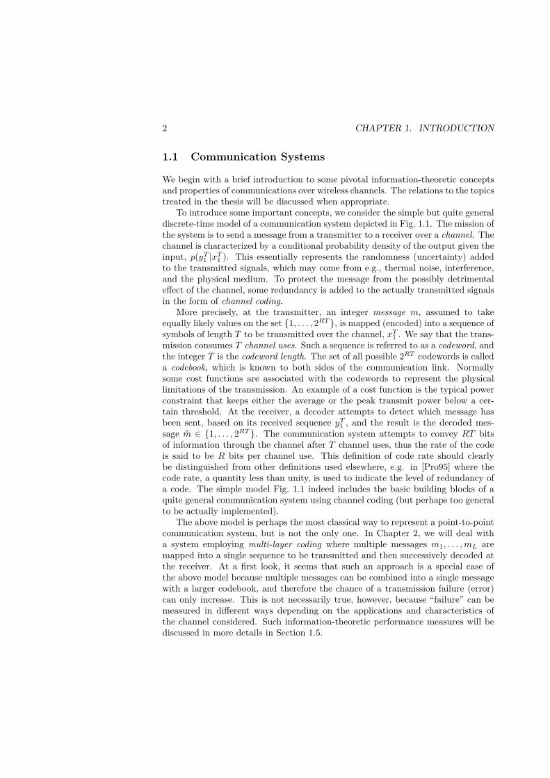
To introduce some important concepts, we consider the simple but quite generaldiscrete-time model of a communication system depicted in Fig. 1.1. The mission ofthe system is to send a message from a transmitter to a receiver over a channel. Thechannel is characterized by a conditional probability density of the output given theinput, p(yT1 |xT1 ). This essentially represents the randomness (uncertainty) addedto the transmitted signals, which may come from e.g., thermal noise, interference,and the physical medium. To protect the message from the possibly detrimentaleffect of the channel, some redundancy is added to the actually transmitted signalsin the form of channel coding.
More precisely, at the transmitter, an integer message m, assumed to takeequally likely values on the set {1, . . . , 2RT }, is mapped (encoded) into a sequence ofsymbols of length T to be transmitted over the channel, xT1 . We say that the trans-mission consumes T channel uses. Such a sequence is referred to as a codeword, andthe integer T is the codeword length. The set of all possible 2RT codewords is calleda codebook, which is known to both sides of the communication link. Normallysome cost functions are associated with the codewords to represent the physicallimitations of the transmission. An example of a cost function is the typical powerconstraint that keeps either the average or the peak transmit power below a cer-tain threshold. At the receiver, a decoder attempts to detect which message hasbeen sent, based on its received sequence yT1 , and the result is the decoded mes-sage m ∈ {1, . . . , 2RT }. The communication system attempts to convey RT bitsof information through the channel after T channel uses, thus the rate of the codeis said to be R bits per channel use. This definition of code rate should clearlybe distinguished from other definitions used elsewhere, e.g. in [Pro95] where thecode rate, a quantity less than unity, is used to indicate the level of redundancy ofa code. The simple model Fig. 1.1 indeed includes the basic building blocks of aquite general communication system using channel coding (but perhaps too generalto be actually implemented).
The above model is perhaps the most classical way to represent a point-to-pointcommunication system, but is not the only one. In Chapter 2, we will deal witha system employing multi-layer coding where multiple messages m1, . . . ,mL aremapped into a single sequence to be transmitted and then successively decoded atthe receiver. At a first look, it seems that such an approach is a special case ofthe above model because multiple messages can be combined into a single messagewith a larger codebook, and therefore the chance of a transmission failure (error)can only increase. This is not necessarily true, however, because “failure” can bemeasured in different ways depending on the applications and characteristics ofthe channel considered. Such information-theoretic performance measures will bediscussed in more details in Section 1.5.

1.2. FADING CHANNELS 3
Channelm m
Encoder DecoderxT1 yT1
p(yT1 |xT1 )
Figure 1.1: A communication system.
1.2 Fading Channels
We will now review the typical characteristics of the physical medium in a wirelessenvironment and relate these to a more specific model of the “channel” in Fig. 1.1.In particular, the additive Gaussian noise model where the transmitted signals,after travelling through a medium, is corrupted by the addition of white Gaussiannoise at the receiver, will be considered. However, one of the most distinguishingfeatures of a wireless channel does not come from the properties of the noise, butfrom the time-varying nature of the underlying physical media.
The time-varying nature of wireless channels is generally governed by two dom-inating terms. The so-called large-scale fading term is caused by path loss andshadowing as the transmit signals travel over distance and get obstructed by largeobstacles [TV05]. This however happens in a much larger time scale (i.e., changingmuch slower) than the duration of a symbol or a codeword. In this work we aremore interested in smaller-scale effects, described as follows.
In a wireless environment, the transmitted signals normally propagate to thereceiver via many different paths. For example, the transmitted signals from a mo-bile station can be reflected from buildings, cars and other obstacles before reachingthe receiver. At the receiver, these signal components may add destructively, asthey undergo different attenuations and arrive at different delays. The fluctuationof received signal strength due to multi-path is known as (small-scale) fading. If thebandwidth of the transmitted signal is much smaller than the coherence bandwidthBm [Pro95] of the channel, all the frequency components of the transmitted signalwill suffer almost the same attenuation and phase shift. Therefore, in this case thechannel is called frequency-nonselective or flat fading. A flat fading channel is wellmodelled as an equivalent time-varying one-tap filter with complex-valued coeffi-cient, illustrated in Fig. 1.2. We usually encounter the case when this coefficient, orchannel gain, is modeled as a zero-mean complex Gaussian random variable. Thisrepresents a rich scattering environment with a lot of reflection paths and no directline-of-sight component. Such a channel is called a Rayleigh fading one because theamplitude of the channel gain is Rayleigh distributed.
On the other hand, when the bandwidth of the transmitted signal is larger thanthe coherence bandwidth, the components that separate more than Bm in frequencywill suffer almost uncorrelated gain and phase offset. The channel in this case iscalled frequency-selective, and is usually modeled as a time-varying tapped delay linewith complex-valued coefficients. Transmission over a frequency-selective channel

4 CHAPTER 1. INTRODUCTION
Channel gain Additive noise
Channel
Figure 1.2: An additive-noise flat fading channel.
results in inter-symbol interference (ISI) and may require complicated equalizationin the time domain. Nowadays, it is generally agreed that a common techniqueknown as orthogonal frequency division multiplexing (OFDM) can often be appliedto convert a frequency-selective channels into a set of parallel narrow-band, flat-fading channels (as usual, under some optimistic assumptions). The thesis thereforefocuses only on the flat fading case.
Fading is traditionally seen as problematic for communication systems, as it maycause significant degradation in the performance, especially in deep fades (when thereceived signal power drops too low to be useful). A conventional method to combatfading is through diversity techniques. The basic idea is to provide several indepen-dent copies of the transmitted signal to the receiver so that the probability that allthese copies simultaneously suffer deep fades is very small. Common diversity tech-niques include time, frequency and space diversity, as well as the combinations ofthese methods. With frequency diversity, the signals carrying the same informationare transmitted on several carrier frequencies. If the separation between any twocarrier frequencies exceeds the coherence bandwidth Bm, then each received versioncan be considered to undergo independent fades. With time diversity, the signalscarrying the same information can be transmitted at different time instants suchthat the time separation between any two copies exceeds the coherence time Td ofthe channel. One way to achieve this in wireless communications is by interleavinga codeword before its transmission.
1.3 Slow Fading
The classification of fading channels into fast and slow ones is critical in order todetermine a suitable information-theoretic performance measure for the system of

1.4. CHANNEL-STATE INFORMATION 5
interest, as will be elaborated in Section 1.5. Throughout this work, the term “slowfading” does not necessarily reflect the speed of change of the underlying physicalmedium like in e.g., [Pro95], but relates to the delay constraints of the transmission.For applications completely insensitive to delay constraint, the receiver can, inprinciple, wait for an unlimited amount of time before attempting to decode. Acodeword therefore can be assumed to span an infinite number of independent fadingblocks. In practice that models a system with a relaxed delay constraint so that itenjoys near perfect interleaving, and thus a codeword can span a large number ofindependent fading states to exploit a significant amount of time diversity. One canthink of downloading a large file for several hours, even days. We will refer to sucha channel as an ergodic one, or less technically, a fast fading channel. On the otherhand, for applications that require a stricter delay constraint such as real-time voiceand video transmission, a codeword can only span a finite, typically small, numberof fading blocks. The length of each fading block, where the channel gain remainsconstant, is typically large enough to average out the effect of noise, thus studyingthe system behavior in the limit of infinite block length still makes sense, eventhough this is seemingly contradicting to the delay-limited assumption [BCT01].We refer to this kind of channel as a slow (or slowly) fading one to distinguishthis from the fast fading case. Furthermore, in this thesis, we exclusively focus onthe extreme case where a codeword spans a single fading block, i.e., the so-calledquasi-static fading channel.
1.4 Channel-state Information
The performance of a communication system is greatly influenced by the assump-tions on the available channel-state information (CSI) at both sides of the links.The term CSI in this thesis refers to the possibly imperfect information about therealization of the channel gain (or a channel matrix in a multi-antenna channel, aspresented later in Section 1.6). We then distinguish between CSI at the transmitter(CSIT) and CSI at the receiver (CSIR).
In both theory and practice, CSIR is considered “easier” to acquire. A typicalway to obtain CSIR is by sending a training sequence known a priori to the receiverso that the it can estimate the channel gain with a certain level of accuracy (as-suming that the channel gain does not change significantly until the next trainingsequence is sent). A thorough analysis of training schemes is presented in [HH03].On the other hand, CSIT is more difficult to obtain. In time division duplex (TDD)systems where uplink and downlink transmission takes place in the same frequency,the reciprocity of the channel can be exploited to estimate the reverse channel gain(provided that the time separation between uplink and downlink slots is consider-ably smaller than the coherence time). The reciprocal properties generally cannotbe exploited in frequency division duplex (FDD) systems, where obtaining CSITrequires some form of feedback.
To simplify the analysis and highlight the effect of partial CSIT, throughout the

6 CHAPTER 1. INTRODUCTION
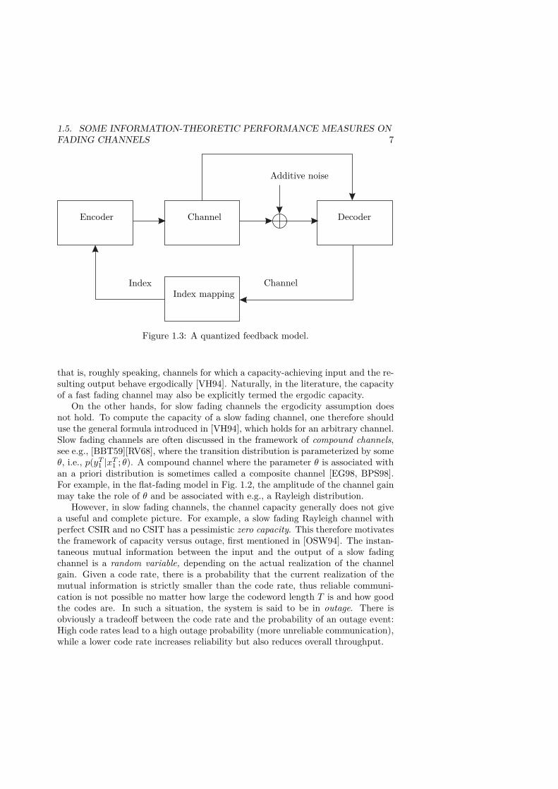
thesis perfect CSIR is always assumed. Of course, in practice, the imperfectnessof CSIR must also be taken into careful consideration because this may lead toremarkable changes in the behavior of some information-theoretic measures [LM03].This thesis exclusively focuses on an explicit quantized feedback model where CSITis obtained via a noiseless, zero-delay dedicated feedback link, depicted in Fig. 1.3.In particular, given a channel gain, the receiver employs an index mapping to obtainan integer feedback index belonging to a finite set {1, . . . ,K} and sends it back tothe transmitter prior to the transmission of a codeword. The constant K is referredto as the feedback resolution. Clearly for that approach to work the transmitter andreceiver must agree on a common strategy with the parameters designed off-line.More realistic assumptions regarding the feedback link should be taken into accountfor any practical system, e.g., the case of noisy feedback link is treated in [JS04].Nevertheless, the feedback resolution that we considered in this work is generallylow (corresponding to 1-2 bits of feedback per fading block) so that the feedbackdelay can be considered insignificant and low-complexity forms of channel codingin the feedback link are also possible, making the zero-delay noiseless feedback linka relatively reasonable assumption.
The explicit quantized feedback model in Fig. 1.3 is not the only model forlimited feedback. Other models may impose different assumptions, for example,that a noisy estimate of the channel is available at the transmitter [JSO02]. An-other line of thought assumes that only the long-term statistics of the channelgain is available at the transmitter, for example, the case of correlated channelswith covariance matrix known at the transmitter is studied thoroughly in e.g.,[VM01, JB04, JG04, VP06]. A hybrid model combining both long-term statisticsand short-term information regarding the channel gain realization is presented in[KBLS06]. There are also the interesting and challenging cases when CSI is notknown by any party of the communication link. Such noncoherent communicationsystems, see e.g., [MH99, ZT02, GS07], are outside the scope of this thesis.
1.5 Some Information-theoretic Performance Measures onFading Channels
Perhaps the most important information-theoretic limitation of a communicationchannel is the channel capacity, introduced in Shannon’s seminal work [Sha48] (seealso [CT91]). Roughly speaking, the capacity C of a channel lets us know theupper limit on the rate of reliable communication over that channel. That is, withan error defined as the event that the transmitter and receiver disagree on whathas been sent, i.e., m �= m in the model in Fig. 1.1, then for any positive numberR < C, it is possible to find codes of rate R that yield arbitrarily small probabilityof error, Pr(m �= m), provided that the codeword length T is sufficiently large.For a memoryless channel, i.e., if p(yT1 |xT1 ) =
∏Ti=1(yi|xi), the capacity is given by
Shannon’s famous maximum-mutual-information formula.Fast fading channels belong to a general class of information-stable channels,
1.5. SOME INFORMATION-THEORETIC PERFORMANCE MEASURES ONFADING CHANNELS 7
Channel
Channel
Index mappingIndex
Encoder Decoder
Additive noise
Figure 1.3: A quantized feedback model.
that is, roughly speaking, channels for which a capacity-achieving input and the re-sulting output behave ergodically [VH94]. Naturally, in the literature, the capacityof a fast fading channel may also be explicitly termed the ergodic capacity.
On the other hands, for slow fading channels the ergodicity assumption doesnot hold. To compute the capacity of a slow fading channel, one therefore shoulduse the general formula introduced in [VH94], which holds for an arbitrary channel.Slow fading channels are often discussed in the framework of compound channels,see e.g., [BBT59][RV68], where the transition distribution is parameterized by someθ, i.e., p(yT1 |xT1 ; θ). A compound channel where the parameter θ is associated withan a priori distribution is sometimes called a composite channel [EG98, BPS98].For example, in the flat-fading model in Fig. 1.2, the amplitude of the channel gainmay take the role of θ and be associated with e.g., a Rayleigh distribution.
However, in slow fading channels, the channel capacity generally does not givea useful and complete picture. For example, a slow fading Rayleigh channel withperfect CSIR and no CSIT has a pessimistic zero capacity. This therefore motivatesthe framework of capacity versus outage, first mentioned in [OSW94]. The instan-taneous mutual information between the input and the output of a slow fadingchannel is a random variable, depending on the actual realization of the channelgain. Given a code rate, there is a probability that the current realization of themutual information is strictly smaller than the code rate, thus reliable communi-cation is not possible no matter how large the codeword length T is and how goodthe codes are. In such a situation, the system is said to be in outage. There isobviously a tradeoff between the code rate and the probability of an outage event:High code rates lead to a high outage probability (more unreliable communication),while a lower code rate increases reliability but also reduces overall throughput.

8 CHAPTER 1. INTRODUCTION
The capacity versus outage framework, however, is not the only performancemeasure for a slow fading channel. For certain applications, it may be better tosplit a message into several ones so that any of them, if successfully decoded at thereceiver, can improve the performance. For example, a coarse version of an imagecan be obtained if some messages are correctly decoded, and a finer, higher-qualityimage can be reproduced if more information is available. It should be clearlyemphasized that such a multi-layer approach is not suitable for many applications.For instance, in data communications an error is declared whenever any layer isincorrectly decoded, thus adding extra layers is generally not an appealing choice.
A frequent performance measure of multi-layer coding is the expected rate.Herein we avoid the term “expected capacity” as used in e.g., [BPS98] and adoptthe more moderate term “expected rate” from [VH94, Cov72] instead. This is bothto avoid confusion with capacity in the traditional sense of the word and to empha-size that, to our knowledge, the multi-layer coding approach has not been shownto be optimal in any sense. Expected rate can be seen as the rate that can becorrectly received, averaged over the randomness of the channel and the noise. Thisis therefore also called reliably received rate in [EG98]. Interestingly, one of themain motivations of Cover’s seminal work on broadcast channels [Cov72] was toimprove the expected rate over a compound channel. This interesting concept hasreemerged recently in [Sha97, SS03], where the asymptotic case with a continuumof layers using differential rate and power is studied. Later, Liu et al. showed thatmost of the gain of infinitely many layers of codes can be realized by a simple two-layer coding scheme for many common channel distributions [LLTF02]. Multi-layercoding is closely related to the study of the capacity region for a general broadcastchannel, a long standing problem in information theory [VH94].
All the aforementioned work assumes perfect CSIR and no CSIT. The presenceof CSIT changes the picture dramatically. For fast fading channels, Goldsmith andVaraiya studied a scalar Gaussian channel with perfect CSI at both sides of the linkand showed that allocating power in a water-filling manner is optimal in a capacitysense [GV97]. However, for most common channel statistics, the benefit of CSIT interms of capacity is not significant, especially at high signal-to-noise ratio (SNR).The achievability part in [GV97] relies on the multiplexing of multiple codebooks.It was later clarified that a simpler combination of a single codebook and a CSIT-dependent power amplifier is sufficient to achieve capacity [CS99]. Furthermore,such a separated structure is optimal even when CSIT is causal and imperfect,under certain assumptions. This holds also for multiple-antenna scenarios, whereCSIT-dependent “transmit weighting” and coding are separated [SJ03].
The presence of CSIT in slow fading channels gives rise to the interesting conceptof power control. If the transmit power can be varied according to the currentchannel gain, outage can be completely avoided even for a strictly positive coderate. Under certain assumptions, this is possible with a finite average transmitpower over infinitely many codewords. In other words, the capacity of such achannel is strictly positive, even though it is a slow fading one. To distinguish thisnotion from the (ergodic) capacity in the fast fading case, this is referred to as delay-

1.6. MULTIPLE-ANTENNA SYSTEMS 9
limited capacity in [HT98, CTB99]. Of course, in connection to the discussion in thissection, delay-limited capacity is precisely the capacity in a traditional (Shannon’s)sense, applied to a special channel model.
1.6 Multiple-antenna Systems
Using multiple antennas is identified as a promising approach to improve the perfor-mance of wireless communications in fading environments. Although space diver-sity has long been utilized by means of multiple receive antennas, only recently hasknowledge about communications with multiple antennas placed at both the trans-mitter and the receiver reached a new level of maturity. Such so-called multiple-input multiple-output (MIMO) systems have been an extremely active researchtopic over the last decade.
Seminal work by Telatar [Tel99] (see also the work by Foschini [Fos96]) showedthat in a system with only CSIR, using Nt transmit antennas and Nr receive anten-nas, where the components of the channel matrix are independent and identicallydistributed (i.i.d.) zero-mean complex Gaussian, the ergodic capacity at high SNRis approximately
C ≈ min(Nr, Nt) log SNR.
That is, in terms of capacity a significant gain of min(Nr, Nt) can be expected athigh SNR compared to a single-antenna system. Unsurprisingly, their promisingresults have sparked great interests in MIMO communications.
A codeword in a MIMO communication system is a matrix, with both spatialand temporal dimensions to be exploited, giving rise to the term space-time coding.In [TSC98], a sufficient condition for a space-time code to achieve “full diversity” ispresented. The developed criterion is quite mild, requiring all codeword differencematrices to be full rank. A surprisingly simple but extremely powerful space-timeblock code for two transmit antennas is introduced by Alamouti in [Ala98]. Amongthe attractive properties of Alamouti’s code are its simplicity in combining and de-coding and its ability to extract the full diversity of the channel. Later, it is shownin [TJC99] that Alamouti’s codes belong to a general class of orthogonal space-timeblock codes (OSTBC). Unfortunately, in [TJC99], it is also shown that “full rate”OSTBC’s using symbols drawn from a complex constellation (such as QAM) do notexist for more than two transmit antennas. Some extensions of OSTBC’s are alsoproposed in [Jaf01], compromising receiver complexity and performance. However,except for the setting of two transmit and one receive antennas, OSTBC’s display aperformance loss compared to the more general linear dispersion codes designed tomaximize mutual information in [HH02], over certain ranges of SNR. Decoding lin-ear dispersion codes generally requires a complicated maximum likelihood receiver(assuming equally likely codewords), or some near-maximum likelihood such as thesphere decoder.
The aforementioned space-time codes are of relatively short length. Combiningmultiple-antenna and more sophisticated error-correcting codes such as trellis codes

10 CHAPTER 1. INTRODUCTION
[TSC98], turbo codes [BGT93], low-density parity check codes [Gal62] and varia-tions such as repeat-accumulate codes also provides significant extra gains. Forfast fading MIMO channels, very close to capacity performance can be achievedwith long random-like codes and joint iterative detection-decoding, see e.g., [SD01,HtB03, tKA04, tK03].
Let us briefly review some work in MIMO channels with some forms of CSIT.In the frontier of fundamental limits, for a constant channel matrix with full CSI atboth sides, a singular value decomposition converts the channel matrix into a set ofparallel spatial channels, and therefore power allocation in a water-filling manneris optimal in a capacity sense [Tel99]. This is readily extendable to fast fadingchannels with full CSI, where water-filling over both time and space is optimal.With limited feedback, capacity results for fast fading channels are reported in[SJ03, LLC04b, LLC04a]. For slow fading channels, the probabilistic power controlframework in [CTB99] is extended to the MIMO case in [BCT01]. Their schemeis not suitable for exploiting time diversity because of a noncausality assumption.The causal case is solved under a dynamic programming framework in [NC02]. Theconcept of minimum rates is independently proposed in [LLYS03] for a single-userchannel and in [JG03] for a broadcast channel, which leads to an interesting solutioncombining both water-filling and channel inversion.
More practical use of partial CSIT in multi-antenna systems has attracted agreat deal of attention recently. Given that a large number of complex channelcoefficients needed to be quantized, it becomes more difficult to “imagine” whatto send back to the transmitter with e.g., 1 bit. Early studies include the de-sign of a precoding matrix influenced by possibly impaired CSIT to improve theperformance of OSTBC’s [JSO02, JS04]. Vector quantization techniques are ap-plied in [NLTW98] to design feedback schemes under different optimization crite-ria. Limited feedback design using an elegant geometrical framework is pursued in[LHS03, LH05, MSEA03].
Cooperative Communications
In certain scenarios, deploying multiple antennas at some parties in a communica-tion link may be difficult or even infeasible due to practical constraints. Interest-ingly, even under such restrictive conditions, it is possible to form virtual antennaarrays by letting these parties cooperate in an intelligent way. While seminal workin this area appeared a long time ago in the context of relay channels [van71, CE79],interests in cooperative communications have only renewed with the series of papers[SEA03a, SEA03b, NBK04, LW03, LTW04, KGG05, HZ05].
Herein we exclusively focus on the classical three-node model of the relay channel[van71, CE79], where a transmitter (source node) communicates with a receiver(destination node) with the help of a relay node that can assume a transmittingand/or a receiving role. Despite the simplicity of the model, the capacity of sucha general relay channel is unknown. In the literature, relaying systems can becategorized as either half-duplex (the relay cannot receive and transmit at the

1.7. DIVERSITY–MULTIPLEXING TRADEOFF 11
same time) or full-duplex (the relay can transmit and receive simultaneously) ones.In this thesis, we exclusively focus on half-duplex channels.
1.7 Diversity–Multiplexing Tradeoff
Most early work on space-time coding either tried to extract a “full” diversity gain[Ala98, TJC99, TSC98], or to achieve “high rates,” e.g., the vertical Bell Labs lay-ered space-time (BLAST) structure [TV05] and the linear dispersion codes [HH02].A new line of thought is pursued in [ZT03], where it is shown that both types ofgains can be simultaneously achieved over a slow fading channel, with a fundamen-tal tradeoff between them. Such an elegantly characterized tradeoff is referred toas the diversity-multiplexing tradeoff, and has sparked a great deal of attention,even if it is rather coarse (defined in the limit of SNR → ∞). Roughly speaking,the diversity gain d lets us know about the asymptotic slope of the error probabil-ity while the multiplexing gain r reflects how large the code rate is compared tothe capacity of a single-antenna channel at high SNR. At high SNR, given a coderate R = r log SNR, an error probability in the order of SNR−d can be achievedwith “good” codes. In other words, this is a high-SNR tradeoff between reliabil-ity and throughput of a multi-antenna system. Notice that the notion of diversitygain in [ZT03] should not be interpreted (in a traditional way) as the number ofindependently faded copies of the transmit signals as seen at the receiver.
The diversity-multiplexing tradeoff is closely related to the theory of error expo-nents [Gal65, Gal68]. Error exponent techniques however involve an optimizationover all probability distributions that is very difficult to solve in general. By re-stricting to a Gaussian distribution and letting the SNR grow unbounded, Zhengand Tse have been able to characterize exactly the asymptotic SNR exponent ofan error event. The key idea is to analyze the asymptotic behavior of the jointprobability density function of the singular values of an i.i.d. complex Gaussianmatrix, under a powerful large-deviations framework.
In the original work [ZT03], it is shown that there exist codes with finite lengththat can achieve the optimal diversity-multiplexing tradeoff. In particular, for achannel matrix of size Nr ×Nt, the codeword length T ≥ Nt +Nr − 1 is sufficientto achieve an error probability that decays as fast as the outage probability does.This is rather surprising, as one may have expected that it is only asymptoticallyachievable with infinitely long codewords. However, that conclusion is based ona random coding argument, with the only practical coding scheme known to bediversity-multiplexing optimal at that time was (again, somewhat surprisingly) thesimple Alamouti’s scheme with a QAM constellation for the 2 × 1 channel. Asan example (from [ZT03]), the diversity-multiplexing tradeoffs achieved by somespace-time codes together with the optimal one over a 2 × 2 channel are plottedin Fig. 1.4. As can be seen Alamouti’s codes are strictly better in a tradeoff sensethan are the simple repetition codes, even though both can achieve “full diversity,”i.e., the diversity at very small rates compared to log SNR. However, none of these

12 CHAPTER 1. INTRODUCTION
0 0.5 1 20
1
4
Multiplexing Gain r
Div
ersi
tyG
ain
d
Optimal TradeoffTradeoff of Alamouti’s CodesTradeoff of Repetition Codes
Figure 1.4: Diversity–multiplexing tradeoff over a 2× 2 channel.
schemes are tradeoff optimal, especially at high multiplexing gains (they cannot beused to achieve “high rates”).
Subsequently, the design of other short-length space-time codes that achieve theentire diversity-multiplexing tradeoff has then quickly become a very active researcharea. Among the first codes designed towards that goal are the lattice space-time(LAST) codes [ECD04] and their variants [ECD06]. To be precise, LAST is stilla random ensemble, albeit is more structured than a Gaussian ensemble and thusallows for more efficient algorithms than a maximum likelihood search such asthe sphere decoding, see e.g., [AEVZ02, JO05]. Even randomly generated LASTcodes are shown to perform very well. In [YW03], Yao and Wornell explicitlyconstructed a family of codes for the 2-transmit-antenna case (Nt = 2), usinga carefully chosen rotation matrix and symbols taken from QAM constellations.Interestingly, they showed that there exist codes of length T = 2 that can achievethe entire tradeoff, for any number of receive antennas Nr ≥ 2, while the Gaussiancoding argument in [ZT03] can only show the existence of codes with length T ≥Nt +Nr − 1 = Nr + 1 in similar settings. One of the key ideas in [YW03] is to finda sequence of codes so that all codeword difference matrices have a nonvanishingor sufficiently slow decaying determinant as the code rate grows. Explicit codedesign based on that nonvanishing determinant criterion is studied extensively, see
1.8. DISTORTION EXPONENT 13
e.g., [BRV05, RBV04, EKP+06]. The D–M tradeoff optimality of these codes canbe explained in the framework of approximately universal codes [TV06], whichcharacterizes codes having all pairwise error probabilities decay exponentially asSNR → ∞, as long as the channel is not in outage. An alternative, geometricinterpretation of such a class of codes together with their applications in MIMOchannels with feedback are presented in [KS07].
The tradeoff between throughput and reliability naturally exists in slow fadingrelay channels. In [LTW04], some basic relaying strategies including AF and DF aredescribed and investigated. The D–M tradeoffs of the schemes studied in [LTW04]show that they are not efficient in the high multiplexing gain regime. Furthermore,it is later clear that these simple schemes are sub-optimal except at zero multiplex-ing gain (i.e., they can achieve the maximum possible diversity gain). In the contextof multiple-relay AF channels, a novel scheme termed as “slotted AF,” which is pro-posed and analyzed in [YB07b], can outperform other known AF protocols in theliterature. An intelligent scheme called dynamic DF is proposed in [AES05]. DDFrelaying uses rateless codes at the source node and one acknowledgement bit fromthe relay node to inform the source when the decoder at the relay succeeds. It turnsout that the D–M tradeoff of this strategy is strictly optimal for all multiplexinggains less than 1
2 . For higher multiplexing gains, while it is unclear whether DDFis still optimal or not, there is no known scheme operating under the same CSIassumptions that can outperforms DDF. Under a much more relaxed assumptionon the CSI that the relay knows both the relay-destination and source-destinationchannel gains, it is shown in [YE07] that compress-and-forward relaying is D–Mtradeoff optimal at all multiplexing gains.
1.8 Distortion Exponent
Inspired by the concept of diversity gains in [ZT03], some researchers have recentlyapplied the main ideas of the D–M tradeoff to the problem of transmitting an analogsource over slow fading channels [CN05, GE05, HG05]. It is noticeable that evenover a simple scalar point-to-point slow fading channel, the celebrated separationtheorem [CT91, Chapter 8] does not hold when the CSI is not fully known at thetransmitter. That is, designing source and channel coding modules separately doesnot necessarily lead to optimal performance. For example, sophisticated hybriddigital–analog (HDA) joint source–channel coding schemes have been shown tooutperform separate coding significantly [MP02, SPA02].
Focusing on source transmission over slow fading MIMO channels with no CSIT,the works in [CN05, CN07, GE05, GE08] quantified the asymptotic behavior of theend–to–end average distortion achieved by different joint source–channel codingschemes in the regime of high SNR. At high SNR, the average distortion behaves asSNR−d
′, bearing a clear similarity to the behavior of the outage probability (and
also the probability of error) when a message is transmitted over the channel. Thequantity d′ is often referred to as the (SNR) distortion exponent, which measures

14 CHAPTER 1. INTRODUCTION
the slope of the average end–to–end distortion on a log-log scale at high SNR.There is a performance tradeoff between the distortion exponent and the so-
called bandwidth ratio b, which is defined as the ratio between the channel band-width and the source bandwidth. The bandwidth ratio b measures the spectralefficiency of the system, with a smaller b reflecting a more efficient schemes thatconsumes less channel bandwidth to transmit a given source. Note that the band-width ratio b does not have any direct connection to the multiplexing gain r in theD–M tradeoff analysis.
The distortion exponent analysis in [CN05, CN07, GE08] provided some freshinsight into the problem of source transmission over slow fading channels. Forexample, in [CN07], it is shown that over MIMO channels a simple HDA scheme isoptimal in the sense that it achieves the best tradeoff between distortion exponentand bandwidth ratio. This optimality however holds only for a range of sufficientlysmall bandwidth ratios, i.e., for highly-compressive systems. In [GE08], a broadcaststrategy where the transmitter sends a layer of codes – as considered in [Sha97] andalso in Chapter 2 – is shown to be optimal in a distortion exponent sense for arange of sufficiently high bandwidth ratios. The transmission schemes for MIMOchannels [GE08] are later extended to the relay settings in [GE07b].
1.9 Contributions and Outline
The common theme of the thesis is the design and analysis of certain communica-tions systems with limited feedback over quasi-static fading channels. The thesis isdivided into three parts, with each part treating a different performance metric.
Part I: Chapter 2
This part deals with the optimization of the expected rate over slowly fading scalarchannels with quantized side information. In particular, we consider a multiple-layer variable-rate system employing quantized feedback to maximize the expectedrate over a single-input single-output slow fading Gaussian channel. The transmit-ter utilizes partial channel-state information, which is obtained via an optimizedresolution-constrained feedback link, to adapt the power and to assign code layerrates, subject to different power constraints. To systematically design the systemparameters, we develop a simple iterative algorithm that successfully exploits re-sults in parallel broadcast channels [Tse97]. We present the necessary and sufficientcondition for single-layer coding to be optimal, irrespective of the number of codelayers that the system can afford. The key observation in this chapter is that un-like in the ergodic case [GV97], even coarsely quantized feedback can improve theexpected rate considerably. Our results also indicate that with as few as one bit offeedback information, the role of multi-layer coding reduces significantly.
The material in this chapter has been published as• T. T. Kim and M. Skoglund. On the expected rate of slowly fading channels

1.9. CONTRIBUTIONS AND OUTLINE 15
with quantized side information. In IEEE Transactions on Communica-tions., volume 55, pp. 820-829, April 2007.
A shorter version also appeared in• T. T. Kim and M. Skoglund. On the expected rate of slowly fading channels
with quantized side information. In Proc. 39th Asilomar Conference onSignals, Systems, Computers, Pacific Grove, CA, October-November 2005.
Part II: Chapters 3, 4, and 5
In Chapter 3, we study a slow fading MIMO channel where the transmitter hasaccess to partial CSIT, which takes the form of log2K noiseless feedback bits. It isassumed that the code rate grows as the long-term average transmit power increases,but does not adapt to the channel state, i.e., a single-rate system is considered. Wefirst characterize the entire tradeoff between the diversity and multiplexing gainsthat can be simultaneously achieved over this channel. Partial power control isshown to be instrumental in achieving the optimal tradeoff over such a system.Our results indicate that the diversity gain can be increased considerably even withcoarsely quantized channel state information, especially at low multiplexing gains.For example, as long as at least one side of the communication link has more thanone antenna, the maximum diversity gain of the system grows exponentially in thenumber of feedback regions.
We then carry out the D–M tradeoff analysis for a variable-rate MIMO systemwith quantized feedback. To make “reliability” more meaningful in this variable-rate setting, the concept of minimum guaranteed multiplexing gain in the forwardlink is introduced and shown to influence the tradeoff remarkably. The resultssuggest that the optimal D–M tradeoff can be achieved by using just two codebooks:one high-rate codebook that determines the multiplexing gain of the system andthe other low-rate codebook that provides the minimum level of quality of service.This holds even if the number of feedback regions is greater than two. Partialpower control allows for a superior diversity gain, which is possible even in thehigh-multiplexing-gain regime.
We then discuss the achievability of the optimal D–M tradeoff by finite-lengthcodes that exist in the literature. In particular, codes that satisfy the approxi-mately universal criterion [TV06] are shown to be also D–M tradeoff optimal in ourpartial-CSIT scenario. We also present a useful geometrical interpretation of theapproximately universal criterion.
Finally, we present two lower bounds to the optimal D–M tradeoff using Gaus-sian random coding argument. Unlike in the original setting (no feedback infor-mation) studied in [ZT03], these lower bounds are only asymptotically tight in thelimit of large block (codeword) lengths. Nevertheless, we show that the new achiev-able bounds can approach the optimal D–M tradeoff closely even with moderatecodeword lengths.
The material in this chapter has been published in

16 CHAPTER 1. INTRODUCTION
• [KS07] T. T. Kim and M. Skoglund. Diversity–multiplexing tradeoff inMIMO channels with partial CSIT. In IEEE Transactions on InformationTheory., volume 53, pages 2743-2759, August 2007.
Conference versions of this work have also appeared in• [KS06a] T. T. Kim and M. Skoglund. Diversity–multiplexing tradeoff of
MIMO systems with partial power control. In Proc. 2006 Zurich Seminaron Communications, Zurich, Switzerland, February 2006.
• [KS06c] T. T. Kim and M. Skoglund. Partial power control. In Proc. 2006IEEE International Conference on Communications, Istanbul, Turkey, June2006.
• [KS06b] T. T. Kim and M. Skoglund. Outage behavior of MIMO channelswith partial feedback and minimum multiplexing gains. In Proc. IEEESymposium on Information Theory, Seattle, WA, July 2006.
Chapters 4 and 5 investigate the D–M tradeoff of three-node scalar relay chan-nels under different assumption of CSI at the source and the relay. Chapter 4 con-siders a relay channel with quantized CSI at the relay and the source. We presenta rather exhaustive study considering many different possible scenarios with quan-tized (channel state) feedback from the relay to source, from destination to relay,and from destination to both source and relay. We show that using one bit from therelay to control the source transmit power is sufficient to achieve the multiantennaupperbound in a range of multiplexing gains. Systems with feedback from destina-tion to control relay transmit power slightly outperform DDF at high multiplexinggains, even with one bit of feedback. Finally, we show that with feedback fromdestination, if the source-relay channel gain is unknown to the feedback quantizerat the destination, the diversity gain only grows linearly in the number of feedbacklevels, in sharp contrast to an exponential growth for MIMO channels as shown inChapter 3.
In Chapter 5 we study a more idealistic channel where the relay node has perfectknowledge about the channel gains of the source-destination and relay-destinationlinks. The motivation of this study is the optimality of the compress-forward relay-ing protocol using Wyner-Ziv (WZ) coding under the same CSI assumptions [YE07].We pose the fundamental question: “How much of the gain in the CF scheme [YE07]comes from the perfect CSIT, and how much comes from WZ coding?” To answerthis question, we quantify the asymptotic loss of compress-forward relaying withsimple quantization at the relay (i.e., without using source coding with side infor-mation as in [YE07]). It turns out that in terms of the D–M tradeoff, the loss ofnot using WZ coding is dramatic. However, we also obtain a more optimistic resultthat using power control at the relay can fully compensate for this loss, as long asthe multiplexing gain is not greater than 2
3 .The material in these chapters has been submitted for possible publication in• [KCS07a] T. T. Kim, G. Caire, and M. Skoglund. Decode-and-forward relay
channels with quantized channel state feedback: An outage exponent analy-sis. Submitted to IEEE Transactions on Information Theory, 2007; revised

1.9. CONTRIBUTIONS AND OUTLINE 17
2008.• [KSC07b] T. T. Kim, M. Skoglund, and G. Caire. Quantifying the loss of
compress-forward relaying without Wyzer-Ziv coding. Submitted to IEEETransactions on Information Theory, 2007.
A short version has been published in• [KCS07b] T. T. Kim, G. Caire, and M. Skoglund. On the outage exponent of
fading relay channels with partial channel state information. In Proc. IEEEInformation Workshop, Lake Tahoe, CA, September 2007.
Part III: Chapters 6 and 7
This part considers the transmission of a continuous-amplitude source over a slowfading channel. We are exclusively interested in the high-SNR regime and theoptimization of the end-to-end expected distortion over the channel.
The main contribution of this part is the investigation of the distortion exponentin the case of limited feedback. Since the distortion exponent analysis essentiallyinvestigates how fast the end-to-end mean square distortion decays to zero and SNRgrows, the study in these chapters is closely related to D–M analysis. There arefundamental differences though. In particular, the end-to-end distortion can be im-proved even under a short-term power constraint (i.e., using only rate adaptation).This is generally not the case for the outage minimization problem. Furthermore,combining power control with rate adaptation yields a superior distortion perfor-mance compared to existing schemes in the literature.
Chapter 6 deals with MIMO channels. We derive upper bounds on the distortionexponents achieved with partial CSIT under a long-term power constraint. It isshown that the exponent achieved with any feedback link of fixed, finite resolutionis bounded above by a polynomial of the product between the number of transmitand number of receive antennas. This behavior can be explained in connection withthe D–M tradeoff results in Chapter 3. The achievable distortion exponent of somehybrid schemes with heavily quantized feedback is then derived. The results showthat dramatic performance improvement over the case of no CSIT can be achievedby combining simple schemes with a very coarse CSIT feedback.
Chapter 6 treats the DF relay channels. It is shown that under a short-termpower constraint, combining a simple feedback scheme with separate source andchannel coding outperforms the best known no-feedback strategies even with only afew bits of feedback information. Partial power control is shown to be instrumentalin achieving a very fast decaying average distortion, especially in the regime ofhigh bandwidth ratios. Performance limitation due to the lack of full channelstate information at the destination is also investigated, where the degradation interms of the distortion exponent is shown to be significant. However, even in suchrestrictive scenarios, using partial feedback still yields distortion exponents superiorto any no-feedback schemes.
The material in these chapters has been submitted for publication as:

18 CHAPTER 1. INTRODUCTION
• [KSC08b] T. T. Kim, M. Skoglund, and G. Caire “On source transmissionover MIMO channels with limited feedback,” submitted to IEEE Transac-tions on Signal Processing, 2008.
• [KSC08a] T. T. Kim, M. Skoglund, and G. Caire. On cooperative sourcetransmission with partial rate and power control. Accepted for publicationin IEEE Journal of Selected Area in Communications, 2008.
A short version has been published in• [KSC07a] T. T. Kim, M. Skoglund, and G. Caire. Distortion exponents over
fading MIMO channels with quantized feedback. In Proc. IEEE Interna-tional Symposium on Information Theory, Nice, France, June 2007.
Contributions Outside the Scope of the Thesis
In addition to the material reported herein, some contributions that are not formallyincluded in the thesis are summarized below.
Combining Linear Precoding and Outer Coding
We propose a simple linear structure to exploit CSIT in a single-user multi-antennasystem. When combined with turbo-coded modulation, the proposed scheme per-forms very close to the capacity limits. With only a few bits per channel use tofeedback CSIT, we can achieve a substantial portion of the possible gain with per-fect CSIT. The converge behavior of the proposed scheme is then analyzed usingextrinsic information transfer charts. Our results show that with the proposedtechnique, a fixed outer code can interact efficiently with the inner detector underdifferent assumptions about the quality of CSIT.
This work has been presented in• [KJS04b] T. T. Kim, G. Jöngren, and M. Skoglund. Weighted space-time
bit-interleaved coded modulation. In Proc. IEEE Information Theory Work-shop, San Antonio, TX, October 2004.
• [KJS04a] T. T. Kim, G. Jöngren, and M. Skoglund. On the convergencebehavior of weighted space-time bit-interleaved coded modulation. In Proc.Asilomar Conference on Signals, Systems, and Computers, Pacific Grove,CA, November 2004.
Limited Feedback Design for Fast Fading MIMO Channels
We propose a transmission scheme combining both short-term and long-term chan-nel state information at the transmitter of a single-user MIMO communicationsystem. Partial short-term CSIT in the form of a weighting matrix is obtainedvia a resolution-constrained feedback link, combined with a unitary transformationbased on the long-term channel statistics. The feedback link is optimized underdifferent power constraints, using vector quantization techniques. Simulations in-dicate the benefits of the proposed scheme in all scenarios considered.

1.10. NOTATION AND ACRONYMS 19
We later extend the vector-quantization-based approach to the case of the down-link (broadcast) channel, to jointly design the scheduler, the (finite) set of precodingmatrices, and the feedback link.
These works have been published in• [KBLS08] T. T. Kim, M. Bengtsson, E. G. Larsson, and M. Skoglund. Com-
bining long-term and low rate short-term channel state information overcorrelated MIMO channels. To appear in IEEE Transactions on WirelessCommunications, 2008.
• [KBLS06] T. T. Kim, M. Bengtsson, E. G. Larsson, and M. Skoglund. Com-bining short-term and long-term channel state information over correlatedMIMO channels. In Proc. IEEE Conference on Acoustic, Speech, SignalProcessing, Toulouse, France, May 2006.
• [KBS07] T. T. Kim, M. Bengtsson, and M. Skoglund. Quantized feedbackdesign for MIMO broadcast channels. In Proc. IEEE International Confer-ence on Acoustics, Speech, Signal Processing, Honolulu, HI, May 2007.
1.10 Notation and Acronyms
In this section we clarify some notation and acronyms used throughout this work.
NotationA A calligraphic uppercase letter denotes a set.x A boldface lowercase letter denotes a vector.X A boldface uppercase letter denotes a matrix.IN Identity matrix of size N .xT The transpose of a vector x.xH The conjugate transpose of a vector x.tr(X) The trace of a matrix X.det X The determinant of a matrix X.‖X‖F The Frobenius norm of a matrix X.X−1 The inverse of a nonsingular matrix X..= The exponential equality, cf. Chapter 3, Section 3.2.x The smallest integer that is not smaller than a (real) scalar x.�x� The largest integer that is not larger than a (real) scalar x.(x)+ Denotes max(x, 0).|A| The cardinality of a set A.A× B The Cartesian product of two sets A and B.E[x] The expected value of a random variable x.

20 CHAPTER 1. INTRODUCTION
AcronymsAF amplify-and-forwardARQ automatic retransmission requestAWGN additive white Gaussian noiseBLAST Bell Labs layered space-timeCF compress-and-forwardCSF channel-state feedbackCSI channel-state informationCSIR channel-state information at the receiverCSIT channel-state information at the transmitterDDF dynamic decode-and-forwardDF decode-and-forwardD–M diversity-multiplexingFDD frequency division duplexHDA hybrid digital-analogi.i.d. independent and identically distributedISI inter-symbol interferenceKKT Karush-Kuhn-TuckerLAST lattice space-timeMIMO multiple-input multiple-outputMISO multiple-input single-outputMMSE minimum mean-square errorOFDM orthogonal frequency division multiplexingOSTBC orthogonal space-time block codesp.d.f. probability density functionQAM quadrature amplitude modulationSIMO single-input multiple-outputSISO single-input single-outputSNR signal-to-noise ratioTDD time division duplexWZ Wyner-Ziv

Part I
Expected Rate
21

Chapter 2
Expected Rate Maximization
In this chapter, we will show how a scalar measure of performance over the slowfading channels that takes into account both the outage probability and the trans-mission rate can be improved using partial channel state feedback. We will studya multiple-layer variable-rate system employing quantized feedback to maximizethe expected rate over a single-input single-output slowly fading Gaussian channel.The transmitter utilizes partial channel-state information, which is obtained via anoptimized resolution-constrained feedback link, to adapt the power and to assigncode layer rates, subject to different power constraints. To systematically designthe system parameters, we develop a simple iterative algorithm that successfully ex-ploits results in the study of parallel broadcast channels. We present the necessaryand sufficient conditions for single-layer coding to be optimal, irrespective of thenumber of code layers that the system can afford. Unlike in the ergodic case, evencoarsely quantized feedback is shown to improve the expected rate considerably.Our results also indicate that with as few as one bit of feedback information, therole of multi-layer coding reduces significantly.
2.1 Introduction
Consider coded data transmission over a slowly fading frequency-flat wireless link.One of the most important performance criteria in this scenario is “throughput”versus “cost” of transmission. Throughput can be measured in many different ways.In this chapter we consider an information-theoretic approach, and will investigatethe “achievable expected rate” over a large number of blocks transmitted at variablerates. The cost of transmission will be measured as either “short-term” or “long-term” average power.
To study capacity and related notions over slowly fading channels one needs tobe specific about the assumed delay-sensitivity of the applications considered. Inapplications completely insensitive to delay, a transmitted codeword can be assumedto span infinitely many independent fading blocks, even over very slowly varying
23

24 CHAPTER 2. EXPECTED RATE MAXIMIZATION
channels. In such delay-unconstrained cases, the ergodic capacity [GV97, Tel99]is a valid performance limit. However, many wireless applications require a strictconstraint on transmission delay. This motivates the block fading Gaussian channelmodel [OSW94], where a transmitted codeword is assumed to span a fixed andfinite number of independent fading blocks. In such scenarios, capacity in thetraditional sense of the term [CT91] is generally not a useful performance measure.For example, a block fading Rayleigh channel has capacity zero, since no positiverates are achievable over this channel [BPS98]. Therefore, other ways to characterizethe channel, for example in terms of throughput versus outage probability [OSW94,CTB99], are often considered in these cases.
When characterizing the achievable performance over a fading channel, oneneeds also to be specific about the available channel-state information. As in mostprevious related works, we will assume perfect CSI at the receiver, motivated bythe separate transmission, at negligible rate-loss, of a training sequence [BPS98].When available, CSI at the transmitter can be utilized to adapt resources andthe transmission strategy and can greatly improve the performance over a slowlyfading channel. A fixed-rate system with non-causal and perfect CSIT, employingpower control based on the CSIT to minimize the outage probability, was studied in[CTB99, BCT01]. These results were then later extended to the causal-CSIT caseusing dynamic programming in [NC02]. A great deal of research has also focusedon systems where the amount of CSIT is positive but strictly limited, the casewe will refer to as partial CSIT. The paper [BSA02] considers a fixed-rate systemand deals with power control to minimize the outage probability based on partialCSIT. On the other hand, [MSEA03] focuses on quantizing the direction of thebeamforming vector of a multiple-input single-output system without performingpower control. Some specific adaptive digital modulation and coding schemes arestudied in [GC97, GC98, VG03, LF00, LYS03, GØH05]. Intelligent use of imperfectfeedback information is also shown to improve various performance measures ofmultiple-antenna systems in e.g., [NLTW98, VM01, JSO02, JS04, LHS03].
While outage probability is a valid measure of the performance of a fixed-rate system over slowly fading channels, for certain applications it may be morereasonable to consider the achievable expected rate over multiple fading blocks[Cov72, BPS98]. Expected rate can also be seen as a measure of reliably decod-able rate, from the receiver’s perspective [EG98]. With perfect CSIR the receiverknows whether the transmission of the present block is in outage, and it can there-fore disregard unreliable blocks. Hence, from the receiver’s perspective, loss ofdata may occur while there will never be any transmission errors. Consequently,all codewords, at rates allocated by the transmitter, are either supported withouterrors or lost. It therefore makes sense to discuss expected rate in the sense ofthe average number of reliably received bits, per channel use over a large numberof transmitted codewords. Interestingly, the traditional outage approach has beenshown to be suboptimal in an expected-rate sense, as higher rates can be achievedusing a broadcast strategy or multi-layer coding [Sha97, SS03, LLTF02]. This ideawas first proposed in Cover’s seminal work on broadcast channels [Cov72]. The
2.2. SYSTEM MODEL 25
multi-layer approach is particularly appealing for, e.g., successive refinement sys-tems, which can produce a coarse version of a source such as an image, when someinformation is available and gradually improve the quality of the reproduced sourceas more information is received.
In this chapter we consider a slowly fading frequency non-selective link withperfect CSIR, and quantized channel feedback information. Our aim is to studythe properties of adaptive systems optimal in an expected-rate sense based on someparticular coding strategies, and with optimized quantizers in the feedback link. Incontrast to a fixed-rate system considered in some previous related works on limitedfeedback, we study a multi-layer variable-rate coding scheme under different powerconstraints. We assume a fairly general framework, valid for any continuous channeldistribution, and we explicitly formulate the feedback design problem. Essentially,quantized CSIT transforms the original channel, which can be viewed as a compositeone [BPS98], into a finite number of parallel composite channels. By exploiting theinherent connection between our design and problems in parallel broadcast channels[Tse97], we develop simple iterative algorithms to optimize the feedback and thepower allocation, as well as some strategy-dependent parameters. This is vastlydifferent from feedback design for an ergodic channel [SJ03, LLC04b] where there isonly a single centroid, namely the power, associated with each quantization region.Furthermore, unlike in the ergodic channel [GV97, LLC04b] where even perfectCSIT improves the ergodic capacity only marginally, our results show that coarselyquantized CSIT provides a significant improvement on the expected rate. With asfew as one bit of feedback information, the role of multi-layer coding is shown todecrease dramatically. Finally, we develop the necessary and sufficient conditionsfor single-layer coding over a conditional channel to be optimal, irrespective of thenumber of code layers that the system can afford.
2.2 System Model
Consider the discrete-time complex-baseband model of a flat-fading single-inputsingle-output communication system illustrated in Fig. 2.1, where the complex-valued channel gain is assumed to be random but constant during one fading blockconsisting of N channel uses. The received signal at time instant t within fadingblock m, m = 1, 2, . . ., can be written as
ym(t) = hmsm(t) + wm(t), t = 1, . . . , N, (2.1)
where hm denotes the channel gain and the sm(t)’s are the transmitted symbols.The noise samples wm(t) are i.i.d. complex Gaussian with zero mean and unitvariance. We assume that the hm’s are i.i.d. according to some distribution. Letγm
Δ= |hm|2, that is the resulting i.i.d. channel powers. In this chapter, we exclu-sively consider the case that any transmitted codeword spans only a single fadingblock. As pointed out in [CTB99, BCT01], it is reasonable to study the case
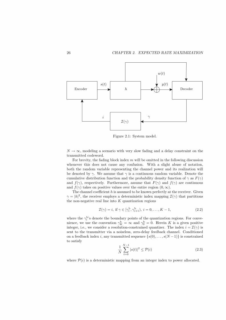
26 CHAPTER 2. EXPECTED RATE MAXIMIZATION
s(t)h
w(t)
y(t)
I(γ)γi
Encoder Decoder
Figure 2.1: System model.
N → ∞, modeling a scenario with very slow fading and a delay constraint on thetransmitted codeword.
For brevity, the fading block index m will be omitted in the following discussionwhenever this does not cause any confusion. With a slight abuse of notation,both the random variable representing the channel power and its realization willbe denoted by γ. We assume that γ is a continuous random variable. Denote thecumulative distribution function and the probability density function of γ as F (γ)and f(γ), respectively. Furthermore, assume that F (γ) and f(γ) are continuousand f(γ) takes on positive values over the entire region (0,∞).
The channel coefficient h is assumed to be known perfectly at the receiver. Givenγ = |h|2, the receiver employs a deterministic index mapping I(γ) that partitionsthe non-negative real line into K quantization regions
I(γ) = i, if γ ∈ [γbi , γ
bi+1), i = 0, . . . ,K − 1, (2.2)
where the γbi ’s denote the boundary points of the quantization regions. For conve-
nience, we use the convention γbK = ∞ and γb
0 = 0. Herein K is a given positiveinteger, i.e., we consider a resolution-constrained quantizer. The index i = I(γ) issent to the transmitter via a noiseless, zero-delay feedback channel. Conditionedon a feedback index i, any transmitted sequence {s(0), . . . , s(N −1)} is constrainedto satisfy
1N
N−1∑t=0|s(t)|2 ≤ P(i) (2.3)
where P(i) is a deterministic mapping from an integer index to power allocated.

2.3. SINGLE-LAYER CODING 27
Denote Pi = P(i), i = 0, . . . ,K − 1. We then consider two different typesof power constraint [CTB99]. The short-term power constraint requires that thepower allocated cannot exceed P , independently of the feedback index, i.e.,
Pi ≤ P, ∀i ∈ {0, . . . ,K − 1}. (2.4)
Under the more relaxed long-term power constraint, the transmitter can adaptthe power based on the feedback index, such that the average power over multipleblocks does not exceed P ,
limM→∞
1M
M∑m=1P(I(γm)) = Eγ [P(I(γ))] ≤ P, (2.5)
where the first equality holds with probability one. This is, in the scenario consid-ered, equivalent to
K−1∑i=0
[F (γb
i+1)− F (γbi )]Pi ≤ P. (2.6)
Due to our assumption of non-zero and continuous density, the channel condi-tioned on a feedback index is still a composite one [BPS98], as in the case of noCSIT, however with a smaller support. That is, the range of uncertainty of theonly partially known γ decreases with the feedback resolution. The coding schemeto maximize the expected rate over such a conditionally composite channel is stillunknown in general. We focus our attention on two specific strategies: the tra-ditional outage approach, which is also referred to as single-layer coding, and thebroadcast strategy or multiple-layer coding. Clearly, single-layer coding is a specialcase of the more general multi-layer coding. We, however, consider this special caseseparately because the problem is more analytically tractable and therefore, moreinstructive. The main challenge is to optimize the index mapper I(γ), the allocatedpower P(i) and some strategy-dependent parameters jointly. In the discussion, weoften refer to the set of all parameters to be designed as a feedback scheme.
2.3 Single-layer Coding
With the single-layer coding approach, given an index i, the transmitter selects acodeword from a rate-Ri capacity-achieving codebook where Ri, i = 0, . . . ,K−1 aredesign parameters. The system is in outage if the instantaneous mutual informationof the channel is smaller than the operating rate Ri [OSW94].
It is convenient to review some results obtained under the assumption of perfectand no CSIT respectively, providing performance bounds to the quantized-CSITsystem of interest. Without any CSIT, the transmitter selects an operating rateof R0 = log(1 + γ0P ) for some γ0. (All logarithms in this chapter are natural,unless otherwise stated.) Since a codeword is successfully decoded only if γ ≥ γ0,

28 CHAPTER 2. EXPECTED RATE MAXIMIZATION
maximizing the expected rate becomes
maxγ0≥0
[1− F (γ0)] log(1 + γ0P ). (2.7)
Setting the first derivative to zero yields a necessary condition for a γ∗0 to be optimal,which we write in the following form for a later reference
1 = F (γ∗0 ) + f(γ∗0 )1 + γ∗0PP
log(1 + γ∗0P ). (2.8)
When perfect CSIT is available, assuming a short-term power constraint, it isclear that for a realization γ, the transmitter should match its rate to the currentrealization of the channel mutual information, i.e., log(1 + γP ), resulting in thefollowing maximum expected rate
R∗S−∞ =∫ ∞
0log(1 + γP )f(γ)dγ, (2.9)
Under the long-term power constraint, the maximum expected rate of the slowlyfading channel is equal to the capacity of an ergodic channel with perfect channelside information [GV97],
R∗L−∞ =∫ ∞λ∗
log( γλ∗)f(γ)dγ, (2.10)
which is obtained by allocating power in a water-filling manner over multiple blocks.The water level 1
λ∗ satisfies∫∞λ∗
(1λ∗ − 1
γ
)f(γ)dγ = P . Intuitively, the transmitter
does not waste power on weak channel realizations and spends the saved power onstrong channel realizations. The gain by optimally allocating power compared theshort-term case is, however, insignificant for many frequently encountered channeldistributions, especially at high SNR [GV97].
Feedback Design Under a Short-term Power Constraint
Let us now focus on the problem of limited feedback design under the short-termpower constraint. It is clear that with a short-term power constraint, the optimalpower P ∗i = P , ∀i, as there is no cost incurred with increasing the power allocatedto each fading block up to the upper limit. Given an index i, the transmitterchooses an operating rate Ri, which is associated with a reconstruction point γi viathe relation Ri = log(1 + γiP ). Since the transmitter knows that the channel cansupport at least a rate of log(1 + γb
i P ) but cannot support any rates larger thanlog(1 + γb
i+1P ), to maximize the expected rate it is necessary that γi ∈ [γbi , γ
bi+1).
If the actual channel power γ ≥ γi, the codeword will be successfully decoded. Onthe other hand, if γb
i ≤ γ < γi, the system is in outage. Designing a feedback

2.3. SINGLE-LAYER CODING 29
scheme optimal in the sense of expected rate is, therefore, equivalent to solving thefollowing optimization problem
max{γi, γb
i}
K−1∑i=0
[F (γb
i+1)− F (γi)]
log(1 + γiP )
s.t. γbi+1 − γi ≥ 0, γi − γb
i ≥ 0.
(2.11)
By a direct investigation of the activeness of the linear constraints, we cansimplify the Karush-Kuhn-Tucker (KKT) conditions for a scheme {γ∗i , γb∗
i } to beoptimal to:
γb∗i = γ∗i , i = 1, . . . ,K − 1 (2.12a)
F (γ∗i+1) = F (γ∗i ) + f(γ∗i )1 + γ∗i PP
log 1 + γ∗i P1 + γ∗i−1P
, i = 0, . . . ,K − 1 (2.12b)
with the convention γ∗−1 = 0, γ∗K = ∞. In the special case of K = 1, i.e., the no-CSIT case, the necessary condition reduces to (2.8). The intuition behind (2.12a)can be explained as follows. Given a fixed set {γ∗i }, the system is in outage ∀γ ∈[γbi , γ∗i ). By increasing γb
i up to γ∗i , we effectively replace the expected rate of zeroin the outage region with R∗i−1 = log(1 + γ∗i−1P ) > 0 and hence, strictly increasethe objective function of (2.11). A direct consequence of (2.12a) is that an outage,defined as the event that the channel cannot support the operating rate, can onlyoccur if the zero index (i = 0) is received at the transmitter.
It is relatively simple to solve for {γ∗i } from (2.12b) since one can expressγ∗1 , . . . , γ
∗K−1, as a function of γ∗0 . (Recall that F (γ) is invertible due to our as-
sumption of non-zero density.) Therefore, (2.12b) with i = K − 1 can be expressedas an equation with a single unknown γ∗0 , which can be solved numerically. Givena γ∗0 (the solution may not be unique), one can successively compute γ∗1 , . . . , γ∗K−1(in that order) using (2.12b). We observe that for many common channel distri-butions, (2.12b) appears to have a unique solution. Furthermore, our experimentsshow that solving (2.12b) directly is much more efficient than using standard opti-mization methods, which generally require a large number of initial random seedsdue to the non-concavity of (2.11).
Feedback Design Under a Long-term Power Constraint
Under the more relaxed long-term power constraint, given an index i, the trans-mitter selects a codeword from a codebook of rate Ri = log(1 + γiPi). In this case,the operating rate Ri depends not only on the reconstruction point γi but also on
30 CHAPTER 2. EXPECTED RATE MAXIMIZATION
the power allocated Pi. The feedback design problem can thus be formulated as
max{γbi, γi, Pi}
K−1∑i=0
[F (γb
i+1)− F (γi)]
log(1 + γiPi)
s.t. P −K−1∑i=0
[F (γb
i+1)− F (γbi )]Pi ≥ 0,
Pi ≥ 0, γbi+1 − γi ≥ 0, γi − γb
i ≥ 0,
(2.13)
which is more challenging than (2.11) due to the non-linear power constraint.Throughout this section, we assume that a constraint qualification holds at themaximizers of (2.13), so that the KKT conditions are necessary-optimality condi-tions [FGW02, BV04]. Let us introduce the Lagrange multiplier λ ≥ 0 associatedwith the power constraint.
Let {γ∗i , γb∗i , P
∗i }K−1i=0 be an optimal scheme and λ∗ be the corresponding optimal
Lagrange multiplier. Note that for any i ≥ 1, γb∗i solves the linearly-constrained
maximization problem
maxx∈[γ∗
i−1,γ∗i
]
[F (x)− F (γ∗i−1)
]log(1 + γ∗i−1P
∗i−1)
− λ∗ ([F (x)− F (γbi−1)]P ∗i−1 + [F (γb∗
i+1)− F (x)]P ∗i).
The sign of the first derivative of the objective function does not depend on x sinceby assumption, f(x) > 0, ∀x > 0. Therefore, we either have γb∗
i = γ∗i−1 or γb∗i = γ∗i .
But if γb∗i = γ∗i−1, the region [γb∗
i−1, γb∗i ) contributes nothing to the expected rate
and neither does the outage region [γb∗i , γ
∗i ). In this case, we can merge those two
regions forming a new scheme with γb�i−1 = γ�i−1 = γ∗i−1, γb�
i = γ�i = γ∗i that achievesthe same expected rate without violating the power constraint. This means that wecan consider γb
i = γi, ∀i ≥ 1 without loss of optimality and focus on the followingdual problem
minλ
max{γi, Pi}
K−1∑i=0
[F (γi+1)− F (γi)] log(1 + γiPi)
− λ(F (γ1)P0 +
K−1∑i=1
[F (γi+1)− F (γi)]Pi
) (2.14)
A simple iterative, Lloyd-like [GG92] algorithm can be developed to obtain asequence of feedback schemes and dual variable {γ(k)
i , P(k)i , λ
(k)}. For simplicity, wewill omit the iteration index k whenever this does not cause any confusion. Givena set {γi} so that γK−1 > · · · > γ0, solving the dual problem (2.14) is equivalent toallocating power over a set of parallel scalar additive white Gaussian noise (AWGN)channels to maximize a linear combination of the achievable rates. The solution is

2.3. SINGLE-LAYER CODING 31
readily obtained by the following water-filling algorithm
P0 =(F (γ1)− F (γ0)F (γ1)
1λ− 1γ0
)+
(2.15a)
Pi =(
1λ− 1γi
)+
i = 1, . . . ,K − 1, (2.15b)
where (x)+ Δ= max(x, 0) and λ is chosen such that the power constraint is active.Since γK−1 > · · · > γ0, there exists an i0 such that Pi > 0, ∀i ≥ i0 and Pi = 0,∀i < i0. In the next step, we fix λ and {Pi} and solve (2.14) for {γi}. Setting thefirst partial derivatives to zero and simplifying leads to
F (γi+1) = F (γi) + f(γi)1 + γiPiPi
[log 1 + γiPi
1 + γi−1Pi−1+ λ (Pi − Pi−1)
], i ≥ i0
(2.16)
which can be solved with the same technique used to solve (2.12b). For i < i0,we can choose some values arbitrarily so that γi > γi−1, ∀i. The two basic stepsdescribed above are iterated until convergence. The procedure is summarized inAlgorithm 1. A natural termination condition for the algorithm is to check whether
R(k+1) − R(k)
R(k+1)≤ ε
where R(k) is the value of the objective function in (2.14) evaluated at {γ(k)i , P
(k)i }
and λ(k), and ε is a small positive number. Selecting the initial values is also animportant issue. It is clear from (2.16) that by choosing P (0)
i = P, ∀i, we canarbitrarily select λ(0). Moreover, with this particular choice of initial values, (2.16)reduces to (2.12b) and the first step in the algorithm is to solve the short-termpower constraint problem. This prevents the algorithm from converging to a localoptimum that is smaller than that obtained under a short-term power constraint.While we do not claim global optimality of the solution due to the non-concavityof (2.13), numerical results indicate that among a large number of random initialvalues, this judicious choice always yields the highest expected rate.
It is also possible to introduce a peak power constraint that limits the powerallocated to any fading block. Such a constraint arises frequently in practice dueto e.g., hardware limitations. In such a case, the design problem can be stated asfollows: Solve (2.13) with the additional constraints Pi ≤ Pm, i = 0, . . . ,K − 1where Pm > P . (If Pm ≤ P , we return to the short-term power constraint case.)By introducing additional Lagrange multipliers, it can be shown that the optimalpower allocation scheme given {γ(k)
i } is a modified version of (2.15a)-(2.15b) wherewe redefine (x)+ Δ= max(min(x, Pm), 0), i.e., water-filling up to Pm is performed.The partitioning step (2.16) still applies in this case.

32 CHAPTER 2. EXPECTED RATE MAXIMIZATION
Algorithm 1: Single-layer Coding with a Long-term Power ConstraintInitialize k = 0, P (0)
i = P , ∀i, arbitrary λ(0);repeat
Fix {P (k)i } and λ(k), solve for {γ(k)
i } using (2.16);Fix {γ(k)
i }, determine {P (k+1)i } and λ(k+1) by the water-filling algorithm
(2.15a), (2.15b) ;k ←− k + 1;
until Convergence ;
2.4 Multiple-layer Coding
A higher expected rate over a composite channel can be achieved by means ofsuperposition coding. This approach exploits the degradedness of scalar AWGNbroadcast channels. The transmitter sends the superposition of L codewords takenfrom L different codebooks, hence the term multi-layer coding. The receiver em-ploys a successive decoder and the amount of data that can be successfully decodeddepends on the actual realization of the channel. The no-CSIT case has been con-sidered in [Sha97, SS03, LLTF02]. Notice that conditioned on perfect CSIT, thetransmitter no longer sees a composite channel, thus the single-layer results (2.9)and (2.10) apply.
Feedback Design Under a Short-term Power ConstraintAssume that L-layer coding is employed over each quantization region. Given afeedback index i, the transmitter sends the superposition of L codewords takenfrom L capacity-achieving codebooks. The rate of codebook j, j = 0, . . . , L− 1, isdesigned so that
Rij = log(
1 + γijPij
1 + γij∑L−1k=j+1 Pik
),
where γij ’s are referred to as the reconstruction points, and Pij is the power con-straint of codebook j. Without loss of generality, assume that γij < γi(j+1), ∀i, j.
Note that the mapping from feedback index to reconstruction points {γij} is one-to-many, meaning that each code layer utilizes the index differently. Herein γij ’s canbe interpreted as the channel powers of L users among infinitely many users of animaginative broadcast channel that the transmitters chooses to communicate with,and Pij ’s can be seen as the power allocated to these users [LLTF02, Sha97, SS03].
The receiver performs successive decoding, i.e., it decodes layer j treating allother layers k, k > j as AWGN. This is possible due to the fact that the distri-bution of the codewords of a capacity-achieving codebook can be considered to beGaussian, in the limit N → ∞ [Cov72, SV97]. Due to the degradedness of thescalar AWGN broadcast channel [CT91] and by definition of Rij , code layer j is

2.4. MULTIPLE-LAYER CODING 33
successfully decoded and subtracted from the received signals if and only if γ > γij .The short-term power problem is, therefore, explicitly formulated as
max{γbi, γij , Pij}
K−1∑i=0
L−1∑j=0
[F (γb
i+1)− F (γij)]
log(
1 + γijPij
1 + γij∑L−1k=j+1 Pik
)
s.t. P ≥L−1∑j=0Pij , Pij ≥ 0, γij ≥ γi(j−1), γ
bi+1 ≥ γi(L−1), γi0 ≥ γb
i .
(2.17)
Similar to the single-layer coding case, it is necessary that γb∗i = γ∗i0, ∀i > 0
for a scheme to be optimal. However, unlike the single-layer case, the necessaryconditions in general cannot be solved directly. Herein we focus on a low-complexityiterative algorithm that successfully exploits results in parallel broadcast channels[Tse97]. We first fix the boundaries of the quantization regions {γ(k)
i0 } and the powerlevels {P (k)
ij } to find the optimal {γ(k)ij }, j > 0. Next {γ(k)
ij } are fixed to find theoptimal power levels. Finally, the newly obtained set of powers and reconstructionpoints is fixed to find new boundaries {γ(k+1)
i0 }. The procedure is summarized inAlgorithm 2 and the details are presented in the following. For clarity, from nowon we omit the iteration indices.
First, given {γi0} and {Pij}, the joint optimization in (2.17) over {γij}, j > 0,decouples into the optimization of each individual γij , which can be done efficientlyusing numerical methods [GMW81]. Next, given {γij}, the optimal Pij ’s can befound separately for each quantization region. Over the quantization region i, theoptimization problem is equivalent to allocating a total power of P to maximize alinear combination of the achievable rates of an L-user scalar Gaussian broadcastchannel, where user j has channel power γij and rate reward
[F (γ(i+1)0)− F (γij)
].
This can be solved by a simple algorithm [Tse97]. In particular, consider the func-tion
J(z) = arg maxj
F (γ(i+1)0)− F (γij)1γij
+ z− λi (2.18)
where z ∈ [0, P ] and
λi = maxj
F (γ(i+1)0)− F (γij)1γij
+ P(2.19)
For any j, the set of all z ∈ [0, P ] such that J(z) = j is shown to be either emptyor a single interval [Tse97]. The length of such an interval is equal to the optimalpower allocated to the code layer associated with γij .
Finally, we need to find optimal {γi0} given {γij}, j > 0 and {Pij}. Thenecessary conditions can be simplified to
F (γ(i+1)0) = F (γi0) + f(γi0) (1 + γi0P )(1 + γi0(P − Pi0))Pi0
(Ri0 −Ri−1) (2.20)
where RiΔ=∑L−1j=0 Rij . Clearly, (2.12b) is a special case of (2.20) where Pi0 = P ,
∀i. Again, we solve (2.20) with standard non-derivative numerical techniques.

34 CHAPTER 2. EXPECTED RATE MAXIMIZATION
Algorithm 2: Multi-layer Coding with a Short-term Power ConstraintInitialize k = 0, {γ(0)
i0 }, {P (0)ij } s.t.
∑j P
(0)ij = P ;
repeatFix {P (k)
ij }, {γ(k)i0 }, find optimal {γ(k)
ij }, ∀j > 0;Fix {γ(k)
ij }, ∀j, find optimal {P (k+1)ij } using (2.18);
Fix {P (k+1)ij }, ∀j and {γ(k)
ij }, ∀j > 0, find optimal {γ(k+1)i0 } using (2.20);
k ←− k + 1;until Convergence ;
Feedback Design Under a Long-term Power Constraint
In this section, we consider the most general case, when multi-layer coding is em-ployed and temporal power control is also possible. The design problem has thefollowing form
max{γbi, γij , Pij}
K−1∑i=0
L−1∑j=0
[F (γb
i+1)− F (γij)]
log(
1 + γijPij
1 + γij∑L−1k=j+1 Pik
)
s.t. P ≥K−1∑i=0
[F (γb
i+1)− F (γbi )] L−1∑j=0Pij ,
Pij ≥ 0, γij ≥ γi(j−1), γbi+1 ≥ γi(L−1), γi0 ≥ γb
i .
(2.21)
Assuming a constraint qualification at the optimal point, we can extend the algo-rithm in Section 2.4 to take into account the Lagrange multiplier λ associated withthe power constraint. As in Section 2.3, we consider only γb
i = γi0, ∀i > 0. Given{γi0}, {Pij}, the set {γij} (for j > 0) can be found similarly to the short-termpower constraint case. The solution does not depend on λ.
Next, for a fixed {γij}, the optimal power allocation and corresponding La-grange multiplier λ can be found with a greedy algorithm for parallel scalar AWGNbroadcast channels [Tse97]. In the currently investigated scenario, we first need tofind the optimal power allocated to each quantization region
Pi =(
maxj
(F (γ(i+1)0)− F (γij)F (γ(i+1)0)− F (γi0)
1λ− 1γij
))+
(2.22)
where λ is chosen such that the power constraint is active. We can then apply(2.18), where λi, i = 0, . . . ,K − 1, is replaced by λ, to find the individual Pij ’s.(The total power assigned to each conditional channel is no longer P .) Note that apeak power constraint can be directly incorporated into (2.22). In this case, eachquantization region is allocated power up to some Pm.

2.4. MULTIPLE-LAYER CODING 35
Finally, given the set {γij} for j > 0, {Pij} and λ, the optimal {γi0} can befound by solving
F (γ(i+1)0) = F (γi0) + f(γi0) (1 + γi0Pi)(1 + γi0(Pi − Pi0))Pi0
· [Ri0 −Ri−1 + λ(Pi − Pi−1)] ,(2.23)
which is a generalization of (2.16). The entire procedure is outlined in Algorithm 3.For the same reasons as in the single-layer coding case, the initial power levels arechosen so that
∑j P
(0)ij = P , ∀i.
Algorithm 3: Multi-layer Coding with a Long-term Power ConstraintInitialize k = 0, {γ(0)
i0 }, {P (0)ij } s.t.
∑j P
(0)ij = P ∀i, arbitrary λ(0);
repeatFix {P (k)
ij }, {γ(k)i0 }, λ(k), find optimal {γ(k)
ij }, j > 0;Fix {γ(k)
ij }, ∀j, find optimal {P (k+1)ij }, λ(k+1) using (2.18), (2.22);
Fix λ(k+1), {P (k+1)ij }, ∀j and {γ(k)
ij }, j > 0, find optimal {γ(k+1)i0 } using
(2.23);k ←− k + 1;
until Convergence ;
Single-layer Optimality ConditionsThe special structure of the feedback problem allows us to obtain some interestingresults. Clearly, it is not necessary that all the coding levels are assigned non-zero power. The following proposition states the necessary and sufficient conditionfor single-layer coding to be optimal, independent of the number of code layersL that the system can afford. More interestingly, we show that if the single-layeroptimality condition is satisfied, then the single reconstruction point must be theleft boundary of the quantization region, i.e., the conditionally worst-case channelrealization.
Proposition 2.1. Consider a quantization region[γbi , γ
bi+1). Suppose that L-layer
coding is employed. For any L ≥ 2, allocating all the available power to a singlereconstruction point is optimal in an expected-rate sense if and only if
γbi ∈ arg max
γ∈[γbi, γbi+1)
[F (γb
i+1)− F (γ)]γ. (2.24)
If (2.24) holds, the optimal reconstruction point that receives all the available poweris γ∗i0 = γb
i .
Proof. See Appendix A.

36 CHAPTER 2. EXPECTED RATE MAXIMIZATION
Intuitively, (2.24) states that the layer corresponding to γbi is the first layer
to be allocated power. However, γbi also corresponds to the weakest layer and
according to [Tse97], this must also be the last layer to be allocated power. Butthe power allocated to each layer corresponds to a single interval, implying thatthe layer γb
i receives all the available power. This is indeed single-layer coding.The condition (2.24) is rather interesting because it only depends on the natureof the channel distribution. As an example, consider a Rayleigh channel with amean channel power of γ, i.e., F (γ) = 1 − exp(−γγ ). One can verify that forany quantization region such that γb
i ≥ γ, (2.24) is satisfied independently of theupper boundary γb
i+1 of the region considered. Hence, upon receiving a feedbackindex corresponding to such a region, the transmitter can employ the traditionalsingle-layer coding without any loss in expected rate.
The condition (2.24) is particularly useful in our proposed iterative procedures.Since the boundaries are known a priori in the iteration steps, the region wheresingle-layer coding is optimal can be quickly determined. The feedback design,however, requires joint optimization of the boundaries and other parameters. Find-ing stronger conditions that hold even if the boundaries are not known a prioriremains an interesting open problem.
2.5 Numerical Results
In Fig. 2.2, we plot the expected rate achieved by several feedback schemes withdifferent numbers of quantization regions and different numbers of code layers overa Rayleigh channel with unit mean power, i.e., F (γ) = 1− exp(−γ). A short-termpower constraint is assumed. The average signal-to-noise ratio is defined as SNR Δ=P/σ2
n = P since the noise variance σ2n is assumed to be unit. Significant gains
can be observed even with coarsely quantized systems. For example, to achievea target expected rate of 2 nats per channel use, feedback schemes with 2 and 4quantization regions require a power of roughly 3 and 5 dB less than a no-CSITsystem does, respectively. Most of the gain of multi-layer coding is observed inthe high-SNR regime. Furthermore, the benefit of multi-layer coding appears to bemore pronounced as the SNR increases. However, as the quality of partial CSITimproves, the role of multi-layer coding reduces substantially. For instance, in asystem with K = 4 quantization regions, there is practically no benefit of using2-layer coding over single-layer coding for any SNR smaller than 30 dB. This canbe attributed to at least two factors. Firstly, as the feedback resolution increases,the support of a conditional channel becomes smaller, hence the “users” of thevirtual broadcast channel experience almost the same channel power. There istherefore little benefit in optimally allocating power among those users. Secondly,we experimentally observed that more quantization regions satisfy the single-layeroptimality condition (2.24) as the feedback resolution increases.
The difference between the expected rates achieved by different schemes andthat achieved by a single-layer coding system under a short-term power constraint

2.5. NUMERICAL RESULTS 37
0 5 10 15 20 25 300
1
2
3
4
5
6
SNR (dB)
Exp
ecte
dR
ate
(nat
s/ch
anne
lus
e)
L = 1. No CSITL = 2. No CSITPerfect CSIT.K = 2. L = 1.K = 2. L = 2.K = 4. L = 1.K = 4. L = 2.
Figure 2.2: Expected rate achieved with different feedback schemes over a Rayleighchannel. A short-term power constraint is assumed.
is plotted in Fig. 2.3. We will refer to this difference as the absolute gain. Ascan be seen, under a short-term power constraint, multiple-layer coding providesan increasing absolute gain as the SNR increases. On the other hand, long-termpower control (with single-layer coding) yields a decreasing absolute gain as theSNR increases. Thus combining multi-layer coding and long-term power controlresults in an interesting effect: The absolute gain appears to be minimum at someintermediate SNR. Another observation is that the most significant absolute gain isobtained when the number of code layers increases from L = 1 to L = 2, a behaviorthat can also be observed in systems without feedback [LLTF02].
To emphasize the promising role of long-term (temporal) power control in sys-tems with very limited power, we plot the expected rate in the low-SNR regionin Fig. 2.4. It should be noted that the SNR range depicted may not be relevantfor some wireless communication systems. Since multi-layer coding only providesa negligible improvement, we only plot the expected rate achieved by single-layercoding. Interestingly, a system controlling transmit power with coarsely quantizedCSIT, namelyK = 2 or 1-bit feedback, outperforms a short-term power constrainedsystem with perfect CSIT for any SNR smaller than −5 dB. Although a long-termpower constraint is clearly more relaxed, the big difference between the quality of

38 CHAPTER 2. EXPECTED RATE MAXIMIZATION
0 10 20 30 400
0.05
0.1
0.15
0.2
SNR (dB)
Abs
olut
eG
ain
(nat
s/ch
anne
lus
e)
L = 2L = 3L = 1L = 2L = 3
Solid curves: Short-term power constraint
Dashed curves: Long-term power constraint
Figure 2.3: Absolute gains (i.e., the gains compared to a single-layer, short-termpower constrained system) over a Rayleigh channel, F (γ) = 1 − exp(−γ). Thefeedback resolution K = 2. Solid and dashed curves correspond to a short-termand a long-term power constraint, respectively.
CSIT (1 bit vs. perfect) makes the comparison sensible. Consequently, the effectsof imposing a peak power constraint on the system is also most pronounced at thisregion, as depicted in Fig. 2.5. As can be seen, when K = 2, a peak power thatis 3 dB higher than the average one severely affects the expected rate. Increasingthe number of quantization regions appears to reduce this effect significantly. Forany K, an optimal scheme tends to allocate power more evenly in the moderateand high SNR region, hence the effect of a peak power constraint diminishes as theSNR increases.
Similar behavior is also observed in some other commonly encountered channels.The performance of various feedback schemes over the equivalent channel of somesingle-input multiple-output (SIMO) systems using maximum ratio combining areplotted in Fig. 2.6. (Clearly, the SISO framework we consider can also be appliedto such SIMO scenarios.)
Numerical results indicate that the proposed algorithms converge relatively fast.As an example, the convergence behavior of the iterative algorithms over a Rayleighchannel is plotted in Fig. 2.7. Note that the convergence speed of Algorithms 2 and

2.6. CONCLUSION 39
−25 −20 −15 −10 −5 0
10−2
10−1
SNR (dB)
Exp
ecte
dR
ate
(nat
s/ch
anne
lus
e)
K = 2. Short-term power constraint.K = 2. Long-term power constraint.K = 4. Short-term power constraint.K = 4. Long-term power constraint.Perfect CSIT. Short-term power constraint.Perfect CSIT. Long-term power constraint.
Figure 2.4: Expected rate achieved over the low-SNR region. Solid and dashedcurves correspond to a short-term and a long-term power constraint, respectively.F (γ) = 1− exp(−γ).
3 depends on the initial values {γ(0)i0 } and {P (0)
ij }. To obtain a “good” startingpoint, we choose P (0)
ij = P/L, ∀i, j and take γ(0)i0 as the boundaries obtained after
several iterations of Algorithm 1, which converges extremely fast. As shown inFig. 2.7, this heuristic approach appears to be reasonably efficient. Experimentswith random seeds also suggest that, at least for the channel distributions presentedin this section, the algorithms lead to convergence to the global optimum. Howeverwe have not been able to prove that analytically.
2.6 Conclusion
We have studied a variable-rate system employing partial CSIT to increase theexpected rate over a slowly fading channel. Our results indicate that a substantialportion of the gain with perfect CSIT can be achieved by heavily quantized CSIT.The improvement provided by the sophisticated multi-layer coding technique isshown to reduce dramatically if the resolution of the feedback quantizer increases.Moreover, in practice, multi-layer coding is also limited by other factors such aserror propagation. This suggests that from an expected-rate perspective, single-

40 CHAPTER 2. EXPECTED RATE MAXIMIZATION
−25 −20 −15 −10 −5 0
10−2
10−1
SNR (dB)
Exp
ecte
dR
ate
(nat
s/ch
anne
lus
e)
K = 2. P m/P = 0 dBK = 2. P m/P = 3 dBK = 2. P m/P = ∞K = 4. P m/P = 0 dBK = 4. P m/P = 3 dBK = 4. P m/P = ∞
Figure 2.5: Effects of a peak power constraint on the expected rate over a Rayleighchannel. Solid and dashed curves correspond to K = 2 and K = 4, respectively.
layer coding may be a suitable choice for systems with feedback, even though someoptimality is lost.
With the same number of quantization regions, optimally allocating power overtime only improves the expected rate marginally at moderate to high SNR’s. Hence,in this region, optimizing the feedback index mapping appears to be more importantthan optimizing the power allocation. On the other hand, in the low-SNR regions,most of the gain comes from temporal power control, which is based on partialCSIT. Therefore, the performance over the low-SNR region is highly affected if apeak power constraint is imposed on the system.
The design of multi-layer coding for MIMO channels is considerably more chal-lenging because channel ordering over such systems is in general not uniquely de-fined. (A particular channel ordering based on majorization theory and a single-dimensional approximation is shown to be inefficient in [SS03].) Nevertheless, aSISO model still applies to a certain multiple-transmit antenna scenarios. For in-stance, the equivalent channel of a MIMO system employing orthogonal space-timecodes is conveniently fitted into a SISO framework.

2.A. PROOF OF PROPOSITION 2.1 41
0 5 10 15 20 25 300
1
2
3
4
5
6
7
8
SNR (dB)
Exp
ecte
dR
ate
(nat
s/ch
anne
lus
e)
L = 1. No CSIT.L = 2. No CSIT.L = 1. K = 2.L = 2. K = 2.Perfect CSIT.L = 1. No CSITL = 2. No CSIT.L = 1. K = 2.L = 2. K = 2.Perfect CSIT.
Figure 2.6: Expected rate achieved with different feedback schemes over SIMOchannels. The channel coefficients are assumed to be i.i.d. zero-mean complexGaussian with unit variance. Solid curves correspond to a 1 × 2 channel. Dashedcurves correspond to a 1× 4 channel. A short-term power constraint is assumed.
Appendix for Chapter 2
2.A Proof of Proposition 2.1
We first need the following lemma.
Lemma 2.1. Consider a quantization region[γbi , γ
bi+1)
and an arbitrary set of Lreconstruction points {γij}L−1
j=0 , where γi0 = γbi . Suppose that (2.24) is satisfied.
Then, the optimal power allocation in an expected-rate sense is P ∗i0 = P , and P ∗ij =0, ∀j > 0.
Proof. (Lemma 2.1) Assume the contrary. Then, according to [Tse97], there existsa γ ∈ (γb
i , γbi+1) and a z > 0 such that
F (γbi+1)− F (γb
i )1γbi
+ z=F (γb
i+1)− F (γ)1γ + z
.

42 CHAPTER 2. EXPECTED RATE MAXIMIZATION
1 2 3 4 5 6 7 8 9 103.14
3.15
3.16
3.17
3.18
3.19
Number of Iterations
Exp
ecte
dR
ate
(nat
s/ch
anne
lus
e)
Algorithm 3
Algorithm 2
Algorithm 1
Figure 2.7: Convergence behavior of the proposed algorithms. F (γ) = 1−exp(−γ).The number of quantization regions K = 2, SNR = 20 dB. The number of codelayers for Algorithm 2 and 3 is L = 2.
However, expressing z as a function of γ leads to
z =[F (γb
i+1)− F (γ)]γ − [F (γb
i+1)− F (γbi )]γbi
F (γ)− F (γbi )
1γγbi
≤ 0
due to (2.24), which is a contradiction.
Assume that (2.24) holds. We need to show that single-layer coding at γbi
is optimal. Let S∗L = {γ∗ij}L−1j=0 be the optimal set of reconstruction points. If
S∗L contains γbi , the asserted result immediately follows Lemma 2.1. Assume now
that the optimal set of reconstruction points does not contain γbi . Let R∗L be the
maximum expected rate achieved by allocating the power P over S∗L. Form a set ofL+1 reconstruction points by adding γb
i to S∗L. Obviously, the maximum expectedrate R∗L+1 achieved by allocating the same power P over the newly formed set canonly be greater than or equal to R∗L. But according to Lemma 2.1, R∗L+1 is achievedby allocating all available power to γb
i , implying that an arbitrary point other thanγbi can be removed from the newly formed (L + 1)-point set without affecting the
expected rate. Thus we have constructed a set of L construction points containing

2.A. PROOF OF PROPOSITION 2.1 43
γbi that achieve R∗L+1 ≥ R∗L. This contradicts to the assumption that the optimalL-point set does not contain γb
i .We complete the proof by showing that if allocating all available power to some
reconstruction point γ ∈ [γbi , γ
bi+1) is optimal for any L, then (2.24) is satisfied.
Assume the contrary, i.e., there exists an γm > γbi such that
γm = min{arg maxγ∈[γb
i,γbi+1)
[F (γb
i+1)− F (γ)]γ}. (2.25)
If γ �= γm, consider optimal power allocation [Tse97] over a set of two recon-struction points {γ, γm}. But (2.25) implies that γm is the first layer to receivepower for any P > 0, which is a contradiction.
Now consider the case γ = γm, i.e., single-layer coding at γm is optimal. Selecta γ ∈ [γb
i , γm) and allocate power over {γ, γm}. Let P (γ) be the solution to the
following equation
F (γbi+1)− F (γm
i )1γm + P (γ)
=F (γb
i+1)− F (γ)1γ + P (γ)
.
Easily see that
P (γ) =[F (γb
i+1)− F (γm)]γm − [F (γb
i+1)− F (γ)]γ
γγm [F (γm)− F (γ)] > 0. (2.26)
This means that the power P (γ) is (optimally) allocated to γm, while all the re-maining power P − P (γ) is allocated to γ. To show a contradiction, it suffices toprove that we can select γ in [γb
i , γm) so that P (γ) is arbitrarily close to zero, and
thus P − P (γ) can be made positive for any P > 0.To that end, note that the first derivative of the objective function in (2.25)
must vanish at γm, i.e.,
F (γbi+1)− F (γm)− γmf(γm) = 0. (2.27)
Using (2.27) and l’Hospital’s rule, we have
limγ→γm
P (γ) = limγ→γm
− [F (γbi+1)− F (γ)− γf(γ)]
γm [F (γm)− F (γ)− γf(γ)] = 0.
(Recall that f(γ) is assumed to be positive for all γ > 0.) This completes theproof.


Part II
Diversity–Multiplexing Tradeoff
45


Chapter 3
D–M Tradeoff in MIMO Channels
In Chapter 2, we have seen that the outage probability and the transmission ratecan be combined into a single performance measure over slow fading channels (i.e.,the expected rate). In this chapter, we will take a closer look at the two-dimensionaltradeoff between the outage probability and the transmission rate. In particular,we derive the diversity–multiplexing tradeoff over a MIMO channel with optimizedresolution-constrained channel state feedback. We will introduce the concept ofminimum guaranteed multiplexing gain in the forward link and show that this sig-nificantly influences the optimal D–M tradeoff. It is demonstrated that power con-trol based on the feedback is instrumental in achieving the D–M tradeoff, and thatrate adaptation is important in obtaining a high diversity gain even at high rates. Acriterion to determine finite-length codes to be tradeoff optimal is presented, lead-ing to a useful geometric characterization of the class of extended approximatelyuniversal codes. With codes from this class, the optimal D–M tradeoff is achievableby the combination of a feedback-dependent power controller and a single code-book for single-rate or two codebooks for adaptive-rate transmission. Finally, lowerbounds to the optimal D–M tradeoffs based on Gaussian coding arguments arealso studied. In contrast to the no-feedback case, these random coding bounds areonly asymptotically tight, but can quickly approach the optimal tradeoff even withmoderate codeword lengths.
3.1 Introduction
Communication over wireless MIMO channels has attracted great interest over thelast decade because, in comparison to traditional single-input single-output systems,MIMO systems promise a better reliability through the use of many independentpropagation paths and a higher throughput through the use of parallel spatialmodes. While most works focus exclusively on one of these two gains, a new lineof thought is introduced in [ZT03], where both types of gain are shown to besimultaneously achievable over a slow fading channel, and the fundamental tradeoff
47

48 CHAPTER 3. D–M TRADEOFF IN MIMO CHANNELS
between these gains is elegantly characterized.Attempts at a characterization of the D–M tradeoff over a multiple-antenna
channel, under the assumption of partial CSIT, are reported in [KS04a, KS05] wherethe feedback information consists of the scalar quantized singular values of thechannel matrix. This assumption is, however, restrictive and the results in [KS04a,KS05] only reflect the asymptotic outage behavior of a particular class of feedbackschemes. An automatic retransmission request (ARQ) scheme for MIMO systemsand its performance tradeoffs are studied in [ECD06]. Such an ARQ system can beviewed as a simple causal feedback scheme using one bit of feedback informationper retransmission round. Combining ARQ with transmit power control [CTB99,BCT01, KS04b], yields a superior tradeoff compared to the no-CSIT case [ECD06].
Direct partial CSIT via resolution-constrained feedback is normally more usefulthan is the indirect channel knowledge provided by an ARQ flag. Furthermore,certain applications that are more sensitive to delay may exclude the possibility ofretransmitting codewords in error. This motivates our present study of the optimaltradeoff between the reliability and rate that can be simultaneously achieved overa MIMO system with resolution-constrained quantized feedback. We advocate anapproach that quantizes the information needed at the transmitter, and not thechannel matrix itself.
We consider two related cases: Single-rate transmission and adaptive-rate trans-mission. For single-rate transmission, the information rate is kept constant andindependent of the CSIT available, a good model for constant bit-rate services. Foradaptive-rate systems, inspired by the notion of minimum rate [LLYS03, JG03],we propose the concept of minimum multiplexing gain to make “reliability” moremeaningful in the limit of high SNR’s. By performing joint power and rate control,and building upon the elegant framework of [ZT03], we derive the optimal D–Mtradeoff in both cases in a recursive manner.
Since partial power control is a key ingredient in achieving the optimal per-formance over slow fading channels with feedback, it is not surprising that thecharacterization of the optimal D–M tradeoff presented in this chapter is similarto that obtained for the ARQ scheme with power control in [ECD06]. The resultsare, however, not equivalent. In particular, we demonstrate that introducing theconcept of minimum multiplexing gain dramatically influences the optimal D–Mtradeoff. Another difference distinguishing the current work from related works liesin the achievability part. More precisely, our achievability proof relies on the exis-tence of a large class of codes, referred here to as extended approximately universalcodes. This class is defined via a (nontrivial) extension of the concepts introducedin [TV06]. We present a simple and useful interpretation of these codes, givingsome novel insight into approximate universality, as studied in [TV06]. Somewhatsurprisingly, we show that if the power constraint imposed on every codeword isreplaced by a more relaxed average power constraint over the whole codebook, thenour extended approximately universal condition does not necessarily coincide withthe well-known non-vanishing determinant criterion [YW03, BR03]. We do not at-tempt to design explicit codes, but instead show that a large class of existing codes

3.2. SYSTEM MODEL 49
can be used to achieve the present optimal D–M tradeoff, when combined with acarefully designed feedback link.
Our results also shed some light into the design of adaptive MIMO systems withsufficiently long codewords at very high SNR. For single-rate systems, the optimalD–M tradeoff can be achieved by a single codebook and a CSIT-dependent powercontroller. On the other hand, an adaptive MIMO system may achieve performanceclose to the optimal tradeoff with only two different codebooks, even if the resolutionof the feedback link is higher.
Finally, to get additional insight, we develop lower bounds on the optimal D–Mtradeoff based on random coding arguments. Interestingly, in contrary to the no-CSIT case where codes drawn from Gaussian ensemble of short length can achievethe entire optimal D–M tradeoff, we show that except for some special cases, Gaus-sian coding arguments do not appear to be sufficient to complete the achievabilitypart when quantized feedback is available. This seems to hold even with carefullyexpurgated codes in combination with optimized feedback schemes. Our randomcoding bounds highlight that for a random code, the gap between the code rate andoptimal feedback threshold is not negligible. Designing a good feedback scheme istherefore a critical task, even in the high SNR regime.
3.2 System Model
Consider the discrete-time complex-baseband model of a frequency-nonselectiveMIMO communication system with Nt transmit antennas and Nr receive antennas.The channel is constant during a fading block consisting of T channel uses, butchanges independently from one block to the next. During a fading block l, thechannel is represented by an Nr × Nt random matrix Hl, and the received signalcan be written in matrix form as
Yl = HlSl + Wl. (3.1)
The components of the temporally and spatially white noise matrix Wl of sizeNr × T are i.i.d. complex Gaussian with zero mean and unit variance, CN (0, 1).The elements of the channel matrix Hl are assumed to be i.i.d. CN (0, 1). Thus weconsider a rich-scattering, Rayleigh fading environment.
It is assumed that the receiver knows the channel matrix perfectly. Given achannel realization, the receiver sends back an index I(Hl) via a noiseless, zero-delay feedback link to the transmitter. Herein I(Hl) is a deterministic mappingfrom a channel matrix to an integer index. With a slight abuse of notation, we alsodenote the random variable representing the feedback index as I, which takes valueson the set {1, . . . ,K} where K is a positive integer, i.e., a resolution-constrainedfeedback link is considered. In other words, the mapping I(Hl) partitions the setof all possible channel realizations into K regions; and priori to the transmissionthe transmitter knows exactly which region the channel matrix belongs to.

50 CHAPTER 3. D–M TRADEOFF IN MIMO CHANNELS
A codeword Sl is assumed to span a single fading block. Since we do not considercoding over multiple fading blocks, the block index l will be omitted whenever thisdoes not cause any confusion. Conditioned on an index I = i, the codeword S istaken from a codebook Ci = {Si(1), . . . ,Si(Mi)} of rate Ri, where all codewordsare equally likely. Herein the Si(k)’s are matrices of size Nt × T .
Define
PiΔ= 1TMi
Mi∑k=1
‖Si(k)‖2F (3.2)
where ‖S‖F denotes the Frobenius norm of matrix S. Note that Pi can be in-terpreted as the average total transmit power conditioned on the event that thefeedback index I = i is received. Since the noise has unit variance, we convenientlytranslate the average transmit power over multiple fading blocks to average signal-to-noise ratio (SNR) and impose a long-term power constraint [CTB99, BCT01]
limL→∞
1L
L∑l=1
1T‖Sl‖2F a.s.= EH[PI(H)] ≤ SNR (3.3)
where the first equality holds with probability one.Note that the index mapping I(H), and the codebooks Ci’s (thus Pi’s and Ri’s)
are all SNR-dependent. In other words, we study a sequence of feedback schemes,one for each value of SNR (cf. [ZT03]). The dependence of the rates on the SNR isexplicitly given by
Ri = ri log SNR, i = 1, . . . ,K,
where the ri’s are some real values in (0,min(Nr, Nt)), independent of SNR. Werefer to ri’s as the individual multiplexing gains, essentially quantifying how largethe rate of each codebook is compared to the capacity of a SISO link at high SNR.
An error occurs when the transmitted codeword is incorrectly detected at thereceiver. Let Pe be the average probability of error (over the randomness of thechannel, the noise and the data). Then the system is said to have a diversity gainof d if
Pe.= SNR−d, (3.4)
where we adopt the following notation of [ZT03]
f.= SNRb ⇔ lim
SNR→∞log f
log SNR = b
where f is a function of SNR.Throughout this work, we focus on the average rate over infinitely many fading
blocks
RΔ= limL→∞
1L
L∑l=1
RI(Hl)a.s.=
K∑i=1
Pr(I = i)Ri.

3.2. SYSTEM MODEL 51
Accordingly, the system is said to have a multiplexing gain of r, also in an averagesense, if
limSNR→∞
R
log SNR =K∑i=1ri lim
SNR→∞Pr(I = i) = r. (3.5)
The main question we try to answer in this chapter is: Over all sequences of schemessubject to the above constraints, which are able to provide a multiplexing gain of r,what is the maximum diversity gain d∗K(r)? We will consider two related problems:
• Single-rate transmission: For each value of SNR, the transmission rate isindependent of the feedback index. In other words, it is constrained that
r1 = · · · = rK = r. (3.6)
This models a system designed to support constant-rate services, such asvoice or video transmission [CTB99, BCT01].
• Adaptive-rate transmission: In a more relaxed setting, the values of r1, . . . , rKcan also be optimized subject to (3.5), i.e., we consider a variable-rate MIMOsystem. In addition, a constraint on the individual multiplexing gains is as-sumed
ri ≥ rmin,∀i ∈ {1, . . . ,K}, (3.7)where rmin is a constant in (0,min(Nr, Nt)), referred to as the minimummultiplexing gain.
The interpretation of (3.7) is that for certain applications, an acceptable quality ofservice is only achieved at a certain minimum rate. Any rate above this thresholdwill enhance the quality of service, thus rate adaptation still makes sense [LLYS03].In the limit SNR → ∞, to be meaningful, the minimum rate should be translatedinto a minimum multiplexing gain. Any fixed minimum rate then becomes a limitingcase, rmin ↓ 0. Furthermore, without imposing (3.7), it is not very meaningful todiscuss outage, i.e., the event that a channel realization cannot support the rate,because a transmitter may, upon accessing to some CSIT, switch off transmissioncompletely. Of course, (3.7) can also be imposed for single-rate transmission, butthe solution is only a simple truncated version of the optimal D–M tradeoff withoutassuming such a constraint. This is not the case for the adaptive-rate problem,where the value rmin heavily influences the optimal D–M tradeoff.
Before proceeding to the derivation of the optimal D–M tradeoff, let us clarifythe notations used throughout the discussion. Throughout this chapter, we definem
Δ= max(Nr, Nt) and n Δ= min(Nr, Nt). For a matrix X, tr X denotes the trace ofX and XH denotes transpose and conjugate. For any π > 0 and ρ > 0, define
I(H, π) Δ= log det(
INr + πNt
HHH)
(3.8)
where the identity matrix of size Nr is denoted as INr , and
F (ρ, π) Δ= Pr (I(H, π) < ρ) (3.9)

52 CHAPTER 3. D–M TRADEOFF IN MIMO CHANNELS
where the probability is over the randomness of the channel matrix.The notation f .= SNR−∞ is used to indicate that the function f of SNR decays
exponentially as SNR→∞ , for example when f = exp(−SNRp) for some constantp > 0. The “exponent inequalities” ≤ and ≥ are explicitly defined as
f ≥ SNRb ⇔ lim infSNR→∞
log flog SNR ≥ b,
f ≤ SNRb ⇔ lim supSNR→∞
log flog SNR ≤ b.
For two sequences f, g of SNR, f .= g ⇔ fg
.= SNR0.
3.3 Outage Upper Bound on the Optimal D–M Tradeoff
An outage event has the interpretation that the conditional channel cannot sup-port the rate RI , even if “Gaussian codebooks” with infinitely long codewords areemployed [OSW94]. For a given feedback scheme, the outage probability, which isalso SNR-dependent, is thus defined as
Pout, KΔ= Pr
(log det
(INr + HQI(H)HH) < RI(H)
)where the positive semi-definite matrices {Qi}Ki=1 correspond to the covariancematrices of the input of the channel conditioned on a feedback index. Outageprobability is relevant to our discussion on the D–M tradeoff because an applicationof Fano’s inequality, similar to that in [ZT03, Lemma 5], yields an upper bound onthe optimal D–M tradeoff
Pe ≥ Pout, K.= SNR−dout,K(r) ≥ SNR−d
∗out,K(r),
for any feedback schemes and any codes of finite length T . Herein −d∗out, K(r)denotes the SNR exponent of the minimum outage probability P ∗out (over all feed-back schemes with resolution K). To find d∗out, K(r), we will, for each given SNR,characterize the resolution-constrained feedback schemes that minimize the outageprobability, and then study the asymptotic behavior of the solution.
Single-rate Transmission
Recall that single-rate transmission means that the constraint (3.6) is imposed.Finding d∗out, K(r) requires a joint optimization over I(H), {Pi}Ki=1, and {Qi}Ki=1where tr(Qi) ≤ Pi. In the limit SNR → ∞, however, it suffices to consider theQi’s to be scaled identity matrices, which are of course dependent on the partialCSIT and the SNR. To see this, note that for any given I(H) and PK1 , by choosingQi
= PiNt
INt and Qi = PiINt , ∀i ∈ {1, . . . ,K}, we obtain the following bounds on

3.3. OUTAGE UPPER BOUND ON THE OPTIMAL D–M TRADEOFF 53
the outage probability,
limSNR→∞
log Pr(log det
(INr + PIHHH) < r log SNR
)log SNR
≤ limSNR→∞
logPout, K
log SNR
≤ limSNR→∞
log Pr(
log det(
INr + PINt
HHH)< r log SNR
)log SNR .
(3.10)
With “regular” power allocation schemes such that Pi.= SNRpi where 0 < pi <
∞, ∀i, it then follows from (3.10) that we can restrict our analysis to the caseQi = Pi
NtINt , ∀i. Intuitively, in the high-SNR regime of interest, allocating the
transmit power evenly over all spatial directions does not affect the SNR exponentof the outage probability 1. We can therefore focus exclusively on the asymptoticbehavior of systems utilizing partial CSIT to control only the transmit power so asto minimize the outage probability. Such a system is completely determined by anindex mapping and a power codebook {Pi}Ki=1, characterized in the following lemma(recall that only deterministic mappings are considered).
Lemma 3.1. For a given SNR and rate R, the outage-minimizing power codebook{P ∗i }Ki=1 solves the following optimization problem
max PK
s.t. [F (R,PK) + 1− F (R,P1)]P1
+K∑i=2
[F (R,Pi−1)− F (R,Pi)]Pi ≤ SNR,
0 ≤ P1 < · · · < PK ,
(3.11)
where F (ρ, π) is defined as in (3.9). The optimal deterministic index mapping isgiven by
I∗(H) ={
1 if I(H, P ∗K) < Rmin{i : i ∈ {1, . . . ,K}, I(H, P ∗i ) ≥ R} otherwise,
(3.12)
where I(H, π) is defined as in (3.8). The minimum outage probability is F (P ∗K).
Proof. Given in Appendix 3.A.
1Indeed, quantizing the direction, i.e., the right singular vectors of the channel matrix[LHS03, MSEA03], provides an SNR gain (somewhat similar to the coding gain of a code) thatis still important in some range of SNR. However, in the current work we are only interested incharacterizing the diversity gain in the framework of the D–M tradeoff, i.e., as SNR→∞.

54 CHAPTER 3. D–M TRADEOFF IN MIMO CHANNELS
Interestingly, the optimal index mapping (3.12) has a “circular” structure wherethe “best” and the “worst” channel realizations share a common index. An eco-nomic interpretation is that if a channel realization is too costly to invert, thesystem should save power for better channel condition. Unlike in the perfect-CSITcase [CTB99, BCT01], however, the optimal transmitter in the limited-feedbackcase does not necessarily switch off transmission, i.e., P ∗1 is generally nonzero. Anintuitive explanation is that switching off transmission requires a zero power levelin the power codebook, which is rather costly given the finite resolution of thefeedback link. This is especially true in the high SNR regime, where switching offtransmission does not save power significantly. Also note that the region associatedwith I∗(H) = 1 is also the only region where an outage event may occur.
It now remains to determine the asymptotic SNR exponent of P ∗K that solves(3.11). Notice that at high SNR, most channel are not in outage, thus some quan-tization regions may become so unlikely that a power level with an SNR exponentstrictly larger than one can be employed without violating (3.3). This motivatesthe following lemma, which determines the SNR exponent of the outage probabilitygiven the asymptotic SNR exponent of the transmit power.
Lemma 3.2. For r ∈ (0, n), let π be a function of SNR such that π .= SNRp wherep is a finite constant and p ≥ 1. We then have
F (r log SNR, π) .= SNR−D(r,p)
where F (r log SNR, π) is defined as in (3.9) and
D(r, p) Δ= infαn1∈A
n∑i=1
(2i− 1 +m− n)αi, (3.13)
where
A Δ={αn1 |α1 ≥ · · · ≥ αn ≥ 0,
n∑i=1
(p− αi)+ < r
}.
Proof. The asserted result is a natural extension of [ZT03, Theorem 4]. We have
F (r log SNR, π) = Pr
⎛⎝ n∑j=1
log(
1 + πNtλj
)< r log SNR
⎞⎠
where λ1 ≤ · · · ≤ λn are the n largest eigenvalues of HHH. By a change of variablesλj = SNR−αj , j = 1, . . . , n, we obtain
F (r log SNR, p) .= Pr
⎛⎝ n∏j=1
SNR(p−αj)+< SNRr
⎞⎠
= Pr
⎛⎝ n∑i=j
(p− αj)+ < r
⎞⎠

3.3. OUTAGE UPPER BOUND ON THE OPTIMAL D–M TRADEOFF 55
where (x)+ Δ= max(0, x). With the λj ’s following a Wishart distribution, an appli-cation of Varadhan’s integral lemma [DZ98, ZT03] (noticing that outage is a rareevent as SNR→∞) yields the asserted result.
The region A only contains αj ≥ 0, ∀j, because outside this region, the outageprobability decays exponentially as SNR → ∞. Also note that the minimizer of(3.13) can be found by a direct investigation:
α∗i =
⎧⎪⎨⎪⎩p for i = 1, . . . , n− J − 1,(J + 1)p− r for i = n− J,0 for i = n− J + 1, . . . , n,
(3.14)
where J Δ=⌊rp
⌋, i.e., the largest integer that does not exceed rp .
We are now ready to state the following theorem, which recursively characterizesthe SNR exponent of the minimum outage probability of a single-rate MIMO systemwith quantized feedback.
Theorem 3.1. The optimal D–M tradeoff of a single-rate MIMO system with Kquantization regions in the feedback link is upper-bounded by the outage bound
d∗out, K(r) = D(r, 1 + d∗out, K−1(r)) (3.15)
where d∗out, 0(r) Δ= 0, ∀r and D(r, p) is defined as in (3.13).
The formal proof, deferred to Appendix 3.B, involves the computation of a lowerbound and an upper bound on d∗out,K(r) that asymptotically match. The lowerbound is obtained by choosing P 1 = SNR
K , P 2 = SNRKF (R,P 1) , . . . , PK = SNR
KF (R,PK−1) ,
implying that the following index mapping together with the power codebook{P i}Ki=1 can be used to achieve the outage bound
I(H) ={K if I(H, PK) < r log SNR,min{i : i ∈ {1, . . . ,K}, I(H, P i) ≥ R} otherwise.
(3.16)
But (3.16) is similar to the power control scheme proposed for the MIMO ARQ[ECD06] and for multiple-input single-output (MISO) channels [BSA02, KS04b]in the sense that the highest power level is used even in the outage region. Ourresult implies that such a non-circular power control scheme is (only) asymptoticallyoptimal in an outage sense. The intuition is that the amount of power saved byusing the truly optimal circular mapping (3.12) goes to zero as SNR→∞.
Some interesting results can be obtained as direct consequences of Theorem 3.1.The first one characterizes the limiting values on the outage bound, highlightingthe fast increase in diversity gain at low rate.

56 CHAPTER 3. D–M TRADEOFF IN MIMO CHANNELS
Corollary 3.1. We have
limr↓0d∗K(r) =
K∑k=1
(NtNr)k
andlimr↑nd∗out, K(r) = 0, ∀K.
Proof. For r sufficiently close to zero and any p ≥ 1, (3.13) is minimized by α∗i = p,i = 1, . . . , n − 1, and α∗n = p − r leading to limr↓0D(r, p) = NtNrp. ApplyingTheorem 3.1, we obtain limr↓0 d∗out, K(r) =
∑Kk=1(NtNr)k, ∀K. It can also be
verified that limr↑nD(r, 1) = 0. Using Theorem 3.1 gives limr↑n d∗out, K(r) = 0,∀K.
The results reveal the fact that in a SISO channel, the maximal diversity gainonly scales linearly with the number of feedback levels K. On the contrary, whenthe system is equipped with multiple antennas, the maximal diversity gain growsexponentially in the feedback resolution K.
The next result explicitly characterizes the outage bound for a channel whereat least one side of the communication link has a single antenna.
Corollary 3.2. If n = 1, the outage bound consists of a single segment between(0,∑Kk=1m
k) and (1, 0).
Proof. For any k ≥ 1, because d∗out, k(r) is a monotonically decreasing functionof r, we have r
1+d∗out, k(r) < 1, ∀r ∈ (0, 1). From (3.14) , we then obtain α∗1 =1 + d∗out, k(r)− r, leading to d∗out, k+1(r) = D(r, 1 + d∗out, k(r)) = m(1 + d∗out, k(r)−r). But d∗out, 1(r) is a single segment, thus d∗out, 2(r), . . . , d∗out, K(r) are all singlesegments.
Adaptive-rate TransmissionA few technicalities need to be taken care of in the adaptive-rate case. One maytry to characterize the optimal index mapping, power and rate allocation for eachSNR as in the previous section. This is however a difficult task, even in the single-antenna case with perfect CSIT [LLYS03], and becomes even less tractable in ourcase due to the joint optimization involving the index mapping. Thus we followanother approach and find an upper bound on the outage bound itself, which isshown to be asymptotically tight, leading to a situation where the single-rate resultscan be reused. The result, proved in Appendix 3.C, is formalized as follows.
Theorem 3.2. For a given rmin ∈ (0, n) and r ∈ [rmin, n), the optimal D–Mtradeoff of a MIMO system with K ≥ 2 quantization regions in the feedback linkand a minimum multiplexing gain rmin is upper-bounded by the outage bound
d∗out, K(r, rmin) = D(rmin, 1 + d∗out, K−1(r, rmin))

3.4. ACHIEVABILITY OF THE OPTIMAL D–M TRADEOFF 57
where d∗out, 1(r, rmin) Δ= D(r, 1), ∀r ≥ rmin.
Essentially, the outage bound is obtained by considering a two-rate system. Therate of one quantization region asymptotically dominates the average multiplexinggain of the system, while power control is employed over the remaining K − 1regions, where the minimum rate is used. The fact that the outage bounds inTheorem 3.2 have a very similar form to those in Theorem 3.1 can be explainedintuitively as follows. The solution to the adaptive-rate problem is an optimalcombination of channel inversion to reduce outage and water-filling to improvethroughput [LLYS03]. At high SNR, the effect of water-filling quickly diminishesand therefore, we essentially reduce to a channel inversion scheme having similarstructure to the single-rate case.
In an extreme case, when rmin ↓ 0, a surprisingly simple outage bound can beobtained, which we loosely refer to as the case of zero minimum multiplexing gain.
Corollary 3.3. The optimal D–M tradeoff of a MIMO system with K ≥ 2 quanti-zation regions in the feedback link and a zero minimum multiplexing gain is upper-bounded by the outage bound
limrmin↓0
d∗out,K(r, rmin) = (NrNt)K−1D(r, 1) +K−1∑k=1
(NrNt)k.
For a given K, the bound in Corollary 3.3 is simply a scaled version of the no-CSIT tradeoff D(r, 1) plus a constant, and therefore is piece-wise linear between thepoints (r = j, d = (NrNt)K−1(Nr − j)(Nt − j) +
∑K−1k=1 (NrNt)k), for j = 0, . . . , n.
Interestingly, the so-called “full diversity gain” NrNt, is already achieved with K =2 at the “maximal” multiplexing gain, i.e., when r ↑ n. However, to obtain thisbound, the multiplexing gains over K−1 quantization regions must approach zero,i.e., some strictly positive, but negligible compared to log SNR, rates are employed.
3.4 Achievability of the Optimal D–M Tradeoff
In this section, we show that the outage bound is achievable, conditioned on theexistence of a general class of codes with finite length. For brevity, we presentthe proof only for the single-rate case and omit the almost identical derivations ofthe adaptive-rate case. The analysis reveals a simple geometrical interpretation ofsuch a class of codes. It turns out that for single-rate transmission, the optimalD–M tradeoff can be achieved by a single codebook and a feedback-dependentpower controller, a combination known to be optimal in different scenarios [CS99,CTB99, BCT01, SJ03]. Connection to approximately universal codes [TV06] andnon-vanishing determinant codes, e.g., in [BR03, EKP+06] among others, will bediscussed.
58 CHAPTER 3. D–M TRADEOFF IN MIMO CHANNELS
Extended Approximately Universal Condition
Consider a sequence of codes C with rate r log SNR (bits per channel use) usingequally likely codewords X(k), k = 1, . . . ,M with M Δ= �SNRrT �, which are ma-trices of size Nt × T , where T ≥ Nt. The average energy of a component in acodeword matrix is normalized such that
1MTNt
M∑k=1
‖X(k)‖2F ≤ 1. (3.17)
For an arbitrary pair of codewords, let μ1 ≤ · · · ≤ μn be the n smallest squared sin-gular values of the codeword difference matrix, and let μj = SNR−βj .We constrainC so that2 ⎛
⎝minC
n∏j=1
SNR−(βj)+
⎞⎠ ≥ SNR−r (3.18)
where the minimization is over all pairs of different codewords in C. Recall that(βj)+ = max(βj , 0). We refer to (3.18) as the extended approximately universalcriterion, because it is related, but not necessarily equivalent to the approximatelyuniversal criterion developed in [TV06]. In the following, we show that the outagebound is achievable by combining C with a CSIT-dependent power amplifier and asuitable index mapping.
Let ε be an arbitrarily small positive number and consider the following indexmapping
I(H) =
⎧⎪⎨⎪⎩
1 if I(H, PK) < (r + ε) log SNR,min{i : i ∈ {1, . . . ,K}, I(H, P i) ≥ (r + ε) log SNR}
otherwise.
where P 1 = SNRK , P 2 = SNR
KF ((r+ε) log SNR,P 1) , . . ., PK = SNRKF ((r+ε) log SNR,P
K−1) . Wethen construct the transmit codewords as
Si(k) =√P iNt
X(k), i = 1, . . . ,K, k = 1, . . . ,M.
where the factor√Pi
Ntis used to guarantee the power constraint (3.3).
For any i ∈ {1, . . . ,K}, consider an arbitrary pair of codewords in C, say X(1)and X(2) and denote ΔX = X(1)−X(2). Also define the ith ε-outage-free regionas
Oεi = {H : I(H) = i, I(H, P i) ≥ (r + ε) log SNR}.2Recall that by our definition of the exponent (“dot”) inequality, the sequence on the left hand
side of (3.18) does not necessarily converge.
3.4. ACHIEVABILITY OF THE OPTIMAL D–M TRADEOFF 59
Clearly, except for i = 1 the second condition defining Oεi is always redundant.The pairwise error probability, that Si(2) is incorrectly detected given Si(1) istransmitted, averaged over the channel, can be upper-bounded by
Pr(
Si(1)→ Si(2),H ∈ Oεi)
≤∫Oεi
exp(− P i4Nt
‖HΔX‖2)f(H)dH
≤∫Oεi
exp
⎛⎝− P i4Nt
n∑j=1λn−j+1μj
⎞⎠ f(λn1 )dλn1 .
The second inequality is due to the worst-case rotation which aligns the orderedsingular values of the codeword different matrix √μj ’s with those of the channel√λj ’s in reverse order [KW03]. Because I(H) and I(H, p) only depend on H viaλn1 , any Oεi is completely characterized by λn1 .
We now compute the asymptotic SNR exponent of the upperbound on thepairwise error probability. By changing variables λj = SNR−αj , μj = SNR−βjand assuming P i
.= SNRpi , we have
∫Oεi
exp
⎛⎝− P i4Nt
n∑j=1λn−j+1μj
⎞⎠ f(λn1 )dλn1
.=∫Oεi
exp
⎛⎝− n∑
j=1SNRpi−(αn−j+1+βj)
⎞⎠ f(αn1 )dαn1
.=∫Bif(αn1 )dαn1 + SNR−∞
where
Bi Δ= Oεi ∩ {αn1 : αn−j+1 + βj ≥ pi, j = 1, . . . , n}
⊂ {αn1 : α1 ≥ · · · ≥ αn,n∑j=1
(pi − αj)+ ≥ r + ε}∩
∩ {αn1 : αn−j+1 + βj ≥ pi, j = 1, . . . , n}.
Thus Bi is essentially a subset of Oεi containing the channel realizations that makethe bound on the pairwise error probability decay sub-exponentially. Note thatalthough Bi can be specified precisely for the Wishart distributed λn1 , we bound itby a larger set that is independent of the distribution of αn1 and will show that thisis sufficient.

60 CHAPTER 3. D–M TRADEOFF IN MIMO CHANNELS
For any αn1 ∈ Bi, we have βj ≥ pi −αn−j+1 leading to (βj)+ ≥ (pi −αn−j+1)+.Thus
n∑j=1
(βj)+ ≥n∑j=1
(pi − αj)+ ≥ r + ε.
However, the condition (3.18) implies that for any ε > 0, there exists an SNR sothat for all SNR > SNR:
n∏j=1
SNR−(βj)+ ≥ SNR−r−ε2 ,
leading ton∑j=1
(βj)+ ≤ r + ε2 ,
meaning that the set Bi is empty for any SNR > SNR, and hence the averagepairwise error probability decays exponentially as SNR → ∞. This holds for anypair of codewords, hence the unionbound on the average error probability gives
Pr(error,H ∈ Oεi) .= SNRTrSNR−∞ .= SNR−∞
for any i and finite codeword length T . Thus, for an extended approximately uni-versal code, the error probability is dominated by the outage event I(H, PK) <(r + ε) log SNR, which by construction of I(H) has asymptotic SNR exponent−d∗out,K(r + ε), with d∗out,K(r + ε) defined as in Theorem 3.1. Therefore
Pe ≤ SNR−d∗out,K(r+ε).
By continuity of d∗out,K(r), the system can achieve points arbitrarily close to theoutage bound as ε ↓ 0. We finally have the following.
Theorem 3.3. If there exists a sequence of codes satisfying the extended approxi-mately universal criterion, i.e., satisfying (3.17) and (3.18), then the optimal D–Mtradeoff of the MIMO channel (3.1) with feedback resolution K and codeword lengthT is given by
d∗K(r) = d∗out, K(r)
for single-rate transmission and
d∗K(r, rmin) = d∗out, K(r, rmin)
for adaptive-rate transmission with minimum multiplexing gain rmin .
The adaptive-rate case can be proved in a similar manner. Interestingly, foradaptive transmission, the optimal tradeoff can be achieved by only two codebooks,leading to an implication for practical applications: At sufficiently high SNR, an

3.4. ACHIEVABILITY OF THE OPTIMAL D–M TRADEOFF 61
0
x2x1
x3
r
(β3)+
Outage-free region
r
(β3)+
(β1)+
(β2)+
Figure 3.1: A geometrical interpretation of the condition (3.18). The channelrealizations making a pairwise error probability decay polynomially are containedin the cuboid, and (3.18) keeps the corners of all the cuboids in the code belowthe surface of the plane x1 + x2 + x3 = r. (The constraints x1 ≤ x2 ≤ x3 are notplotted to improve readability.)
adaptive MIMO system may not need too many different code rates to achieveperformance close to the optimal tradeoff. Indeed, using two code rates is sufficient.The higher rate asymptotically dominates the average multiplexing gain of thesystem, while the lower rate guarantees the minimum level of quality service in poorchannel conditions. Notice however that the D–M tradeoff result is an asymptoticanalysis, thus for low and moderate SNR, that conclusion does not necessarily hold.
Discussion
The condition (3.18) has a simple geometrical interpretation, illustrated in Fig. 3.1.Let xj = (pi − αj)+ ≥ 0. The set of all xn1 in the nonnegative orthant so that∑nj=1 xj ≥ r + ε contains the ε-outage-free region. On the other hand, the set

62 CHAPTER 3. D–M TRADEOFF IN MIMO CHANNELS
of all “bad” channels that make the pairwise probability decay sub-exponentiallyis contained in the cuboid defined by 0 ≤ xj ≤ (βj)+, where the βj ’s correspondto the SNR exponents of the squared singular values of an arbitrary codeworddifference matrix. By keeping the corners of any such cuboid below the surface ofthe hyperplane
∑nj=1 xj = r, the condition (3.18) guarantees that all pairwise error
probabilities decay exponentially as SNR→∞ .Having all pairwise error probabilities decay exponentially in the limit SNR→
∞ as long as the channel is not in outage, regardless of the channel distribution,is called the approximately universal property in [TV06]. In [TV06], the necessaryand sufficient conditions for a code to be approximately universal are established,assuming no CSIT (Pi = SNR) and under a power constraint on every codeword (anindispensable assumption for their results to hold). In this chapter, we relax thisassumption and approach the problem within the framework of quantized feedback,giving some new insight. Furthermore, by tailoring the universality condition to theproblem at hand, we obtain a stronger result, that the optimal D–M tradeoff canbe achieved by a single code together with a power amplifier, which only dependson the feedback index.
For completeness, in Appendix 3.D we show that (3.18) cannot be relaxed toadmit more codes that is approximately universal for any sequence of channel dis-tributions, even though such a necessary condition is not the main focus of thischapter. However, this (very) strong requirement may not be necessary to achievethe optimal D–M for a particular channel distribution. This motivates our fur-ther study on the achievable tradeoffs of codes drawn from random ensembles inSection 3.5.
Relations Between Different Criteria
If replacing (3.17) with a more stringent power constraint imposed on every code-word
1TNt‖X(k)‖2F ≤ 1, ∀k, (3.19)
then with any SNR we have μj = SNR−βj ≤ TNt, ∀j for any pair of codewords.The approximately universal condition in [TV06], obtained under (3.19), can bewritten as ⎛
⎝minC
n∏j=1
SNR−βj⎞⎠ ≥ SNR−r. (3.20)
When n = Nt ≤ Nr, (3.20) is obviously equivalent to the non-vanishing determinantcriterion (NVD) [BR03, YW03, EKP+06], which requires⎛
⎝minC
Nt∏j=1
SNR−βj⎞⎠ ≥ SNR−r. (3.21)

3.4. ACHIEVABILITY OF THE OPTIMAL D–M TRADEOFF 63
However, for n = Nr < Nt, (3.20) and (3.21) are not equivalent. A code satisfyingthe stronger NVD criterion (3.21) also satisfies (3.20), but not vice versa.
Under (3.17), the arguments in [TV06] generally do not hold because the eigen-values of a codeword difference matrix are not bounded. Our results show thatunder a less restrictive power constraint, (3.20) should be further relaxed to (3.18).Furthermore, any code that has the property (3.20) under (3.19) also satisfies theweaker requirement (3.18), because⎛
⎝minC
n∏j=1
SNR−βj⎞⎠ (3.19)≤ (TNt)n−n
⎛⎝minC
n∏j=1
SNR−βj⎞⎠
.=
⎛⎝minC
n∏j=1
SNR−(βj)+
⎞⎠
where n is the integer such that βn ≥ 0 and βn+1 < 0. Interestingly, even if n = Nt,the product
∏nj=1 SNR−(βj)+
is no longer equal to the determinant of a codeworddifference matrix if that codeword difference has some very large singular values.Somewhat surprisingly, the condition (3.18) implies that having such an abnormallylarge codeword difference with energy much larger than the noise variance (in anorder of magnitude sense) does not really help, as only the nonnegative parts ofβj ’s count. On the other hand, finding codes belonging to the larger class definedby (3.18) may be an easier task. Besides, it is more helpful to use (3.18) whenworking with random codes, as will be shown in Section 3.5.
A remaining and very important question is: Does such a constrained code(3.18) exist for MIMO channels? A number of codes are known to satisfy (3.20)as presented in [TV06], for example QAM for single transmit-antenna, Alamouti’sscheme with QAM constellations [Ala98] for 2 × 1 channels and, tilted QAM fortwo transmit antennas [YW03], Golden codes [BRV05] for 2 × 2 systems. For acertain numbers of transmit antennas, codes presented in [RBV04, ORBV06, KR05]satisfy (3.21). Consequently, all the aforementioned codes can achieve the optimalD–M tradeoff presented herein. The strongest claim to date, based on an explicitconstruction, states that there exist codes of length T ≥ Nt satisfying (3.21) for anyNt [EKP+06]. Their existence completes the achievability part, i.e., the optimalD–M tradeoffs of MIMO systems with feedback resolution K coincide with thecorresponding outage bounds for any T ≥ Nt.
Numerical ExamplesThe tradeoffs for single-rate and adaptive-rate (with a near zero minimum multi-plexing gain) systems are compared in Fig. 3.2. As can be seen, even a few bitsof feedback information can increase the diversity gain of a MIMO channel dra-matically. A large improvement in the diversity gain can be observed in all cases,even with coarsely quantized feedback. This suggests that from a diversity gain

64 CHAPTER 3. D–M TRADEOFF IN MIMO CHANNELS
0 1 20
50
85
Multiplexing Gain
Div
ersi
tyG
ain
K = 3
K = 2
No CSIT, K = 1
Solid: Adaptive-rate (rmin = 0.001).Dashed: Single-rate.m = n = 2.
Figure 3.2: D–M tradeoffs of single-rate and adaptive-rate (rmin = 0.001) transmis-sion over a 2× 2 channel with different feedback resolution K.
perspective, increasing the feedback resolution can be more efficient than addingantennas, provided that transmit power control is possible. The intuition behindthis “power-control diversity” is that we can isolate certain “bad” channels into re-gions with polynomially small probability measures and employ polynomially largepowers over those regions without violating the power constraint (cf. also [ECD06]).This gives “diversity on top of diversity.” The effect can be interpreted as time di-versity even though we only code over a single fading block: Transmit power issaved over a long time period to be used in a few rare peaks.
As illustrated in Fig. 3.2, the penalty of keeping the rate independent of thefeedback index is relatively large, especially at high multiplexing gain. More im-portantly, it is possible to achieve nonzero diversity gain with rate adaptation, evenat the “maximal” average multiplexing gain. For a given resolution K, the twocurves coincide at zero multiplexing gain, where the multiplexing gain is not theparameter of interest. Thus rate adaptation is essential to achieve a high through-put together with a nonzero diversity gain.
The D–M tradeoff over a 4×4 channel with different minimum multiplexing gainsis plotted in Fig. 3.3. Clearly, increasing the minimum threshold on the individual
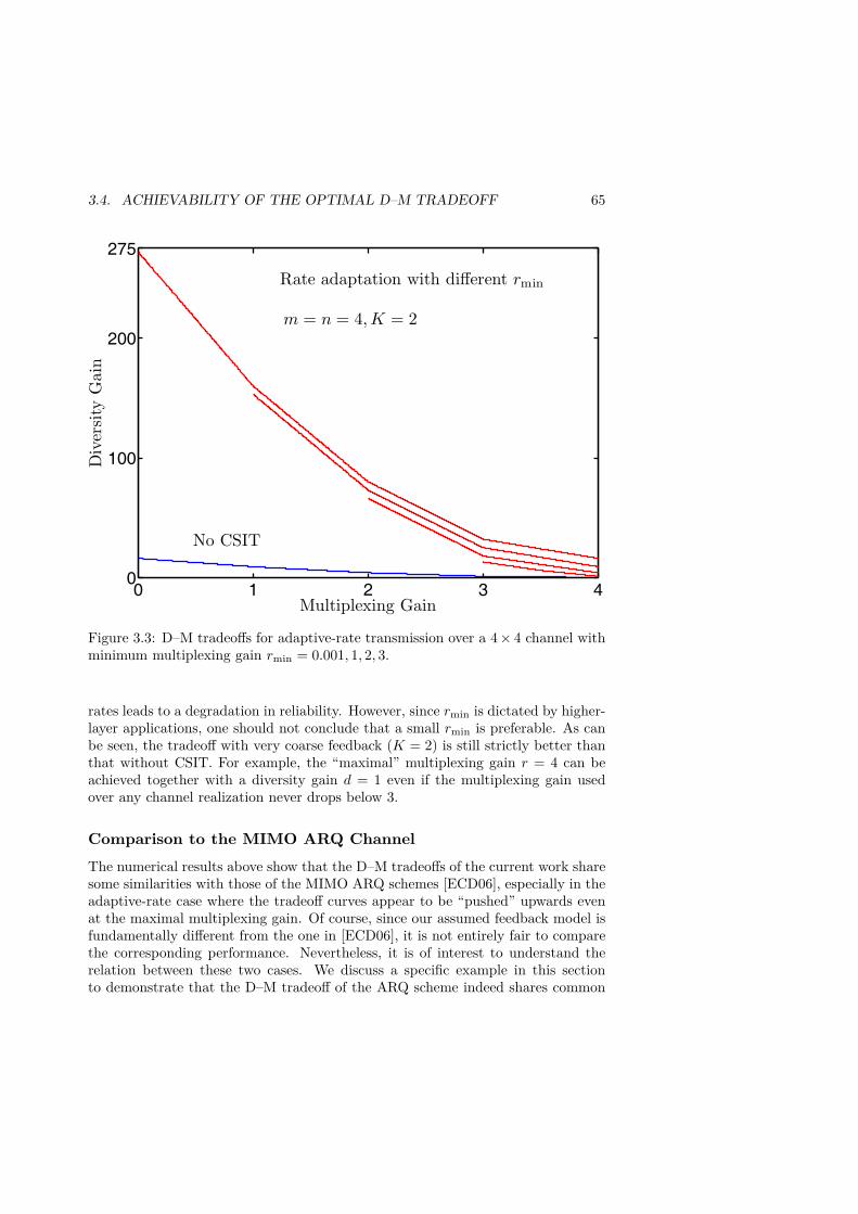
3.4. ACHIEVABILITY OF THE OPTIMAL D–M TRADEOFF 65
0 1 2 3 40
100
200
275
Multiplexing Gain
Div
ersi
tyG
ain
No CSIT
m = n = 4, K = 2
Rate adaptation with different rmin
Figure 3.3: D–M tradeoffs for adaptive-rate transmission over a 4× 4 channel withminimum multiplexing gain rmin = 0.001, 1, 2, 3.
rates leads to a degradation in reliability. However, since rmin is dictated by higher-layer applications, one should not conclude that a small rmin is preferable. As canbe seen, the tradeoff with very coarse feedback (K = 2) is still strictly better thanthat without CSIT. For example, the “maximal” multiplexing gain r = 4 can beachieved together with a diversity gain d = 1 even if the multiplexing gain usedover any channel realization never drops below 3.
Comparison to the MIMO ARQ Channel
The numerical results above show that the D–M tradeoffs of the current work sharesome similarities with those of the MIMO ARQ schemes [ECD06], especially in theadaptive-rate case where the tradeoff curves appear to be “pushed” upwards evenat the maximal multiplexing gain. Of course, since our assumed feedback model isfundamentally different from the one in [ECD06], it is not entirely fair to comparethe corresponding performance. Nevertheless, it is of interest to understand therelation between these two cases. We discuss a specific example in this sectionto demonstrate that the D–M tradeoff of the ARQ scheme indeed shares common

66 CHAPTER 3. D–M TRADEOFF IN MIMO CHANNELS
characteristics with both single-rate and adaptive-rate scenarios.We will compare a power-controlled ARQ channel having an effective multiplex-
ing gain of r and no more than LR rounds of transmission (the channel matrix isunchanged during all rounds) to an adaptive-rate system with multiplexing gain r,feedback resolution LR and minimum multiplexing gain rmin = r
LR. This is because
the worst channel conditions require all LR rounds, and thus the smallest “instan-taneous” multiplexing gain of the ARQ scheme is only r
LR. In addition, the power
codebooks of both systems are of size LR. Note that for the sake of comparison,we constrain the adaptive-rate system to have a minimum multiplexing gain rminthat is dependent on r.
The explicit form of the D–M tradeoff for a power-controlled MIMO ARQ systemis difficult to compute in general [ECD06]. To get some insight, we study the casen = 1 (e.g., an m× 1 MISO channel) where closed-form expressions can be workedout. Let the channel vector be h. Then the outage event in the MIMO ARQscheme [ECD06] is given by
log(
1 + PARQ1Nt‖h‖2F
)+ . . .+ log
(1 +PARQLR
Nt‖h‖2F
)
< r log SNR.(3.22)
For the adaptive-rate system, the outage event is
log(
1 +P adapLR
Nt‖h‖2F
)<r
LRlog SNR. (3.23)
Note that the SNR exponents of the power levels in the two schemes are recursivelycomputed. While PARQ
1.= P adap
1.= SNR and PARQ
2.= P adap
2.= SNR1+m−mr, this
exponential equality does not hold for an arbitrary pair PARQk and P adap
k . Indeedthe adaptive-rate system has a higher power level for any k ≥ 3, as discussed inObservation 2 below.
From (3.22), the D–M tradeoffs of the ARQ channel, denoted as dARQLR
(r), canbe computed. Let us find dARQ
LR(r) explicitly for the first few values of LR. For
LR = 2 we have
dARQ2 (r) =
{(m+m2)(1− r) if r < m
m+1 ,m(m+2)−m(m+1)r
2 otherwise.
For LR = 3 and m > 1 we have
dARQ3 (r) =
{(m+m2 +m3)(1− r) if r < m
m+1 ,
m(
1− r + m(m+2)−m(m+1)r2
)otherwise.

3.4. ACHIEVABILITY OF THE OPTIMAL D–M TRADEOFF 67
0 0.5 10
5
10
14
Multiplexing Gain
Div
ersi
tyG
ain
Solid: Rate adaptationDashed: ARQ
LR = 3
LR = 2
LR = 1 (No CSIT)
Figure 3.4: Comparison of an adaptive-rate system and the power-controlled MIMOARQ scheme [ECD06] over a 2× 1 channel.
For m = 1, i.e., a SISO channel, the result for LR = 3 is slightly different:
dARQ3 (r) =
⎧⎪⎨⎪⎩
3− 3r if r ∈ (0, 12 ],
9−6r4 if r ∈ ( 1
2 ,56 ],
11−6r6 otherwise.
The D–M tradeoff of the adaptive-rate system in this n = 1 case is found to be(cf. Theorem 3.2)
d∗LR
(r,r
LR
)=(m+m2 + . . .+mLR
)−mLRr − (m+ . . .+mLR−1) r
LR.
In Fig. 3.4 the D–M tradeoffs of both the ARQ scheme and the adaptive-rate systemin the case m = 2 are plotted.
We summarize the discussion above in the following two observations.

68 CHAPTER 3. D–M TRADEOFF IN MIMO CHANNELS
Observation 1: The first (leftmost) segment of the ARQ tradeoff coincidesexactly with the D–M curve d∗LR
(r) of the single-rate system with LR feedback levels(cf. Theorem 3.1). The intuition behind this remarkable phenomenon is that for asufficiently small r, the h’s that dominate the outage exponent must be in very deepfades such that the first LR−1 rounds of transmission are completely “wiped out” bythe channel in the sense that (1+PARQ
i ‖h‖2F) .= SNR0, i = 1, . . . , LR−1. Thus thefirst LR−1 transmission rounds do not contribute anything to the SNR exponent ofthe outage probability. Since only the last block of transmission (round LR) makesan impact on the outage exponent, it is then clear from (3.22) that the D–M tradeoffof the ARQ system is equivalent to that of the single-rate system investigated inSection 3.3. We notice that this fact is also consistent with a numerical observationin [ECD06] when lower bounds to the optimal D–M tradeoff are computed.3
Observation 2: The adaptive-rate system has a higher diversity gain at allmultiplexing gains. This can be explained intuitively by comparing (3.22) and(3.23). Because the causal-feedback ARQ scheme keeps trying higher power levelsand longer codeword lengths (i.e., lower rates), in the outage event (3.22) eachpart of the ARQ codeword experiences a different power level. On the other hand,with noncausal knowledge about the channel state, the adaptive-rate scheme canimmediately switch to a small-rate codebook and a high power. Therefore in theoutage event the whole codeword experiences the largest power level as in (3.23),leading to a higher diversity gain.
Since the power levels are computed recursively, this effect is magnified as LRgrows. That is, the performance gap between rate adaptation and ARQ widensas the maximum number of transmission rounds increases. On a final note, for agiven LR, both ARQ and rate adaptation provide the same maximal diversity gain.Given the discussion in Observation 1, we can say that this is simply due to thefact that single-rate and adaptive-rate curves coincide in the limit r ↓ 0.
3.5 Lower Bounds on the Optimal D–M Tradeoff: GaussianCoding Bounds
There are several reasons to study the achievable D–M tradeoff with codes drawnfrom a random ensemble. First, the strong codes satisfying the extended approxi-mately universal criterion (3.18) may not be necessary to achieve the optimal D–Mfor a particular channel distribution. Furthermore, in the no-CSIT case, even Gaus-sian codes of very short lengths can achieve the optimal D–M tradeoff, inspiringsome important classes of low-complexity codes such as Lattice Space-Time codes
3This suggests that for sufficiently low multiplexing gains, a simple repetitive power-controlledARQ scheme, where the transmitter keeps sending the same codeword with higher and higherpower levels until success or deadline and where the receiver decodes based on the latest roundonly, is D–M tradeoff optimal. Intuitively, the gain from power control at low multiplexing gainsis so large that it masks out the effects of reducing the code rate (which is already small from thefirst round).
3.5. LOWER BOUNDS ON THE OPTIMAL D–M TRADEOFF: GAUSSIANCODING BOUNDS 69
and their variations for the ARQ channels [ECD04, ECD06]. In this section, we de-velop two lower bounds on the optimal D–M tradeoff with Gaussian random codes.These bounds are nontrivial generalization of their counterparts in the no-CSITcase [ZT03], and their derivations are considerably different due to the presenceof quantized CSIT. It turns out that, except for some special cases, the boundsare only asymptotically tight, which is quite surprising given the result of [ZT03].Nevertheless, the derived lower bounds quickly approach the outage upper boundeven for very moderate codeword lengths. Our results give some insight into theapproximate universality of codes drawn from Gaussian ensembles, as well as intothe D–M performance of random codes in the presence of CSIT.
Back-off BoundsThe key idea of back-off bounds is to feedback when the channel is good enoughto support a strictly larger rate than the transmission rate, hence the term “back-off.” By exploiting the gap between the code rate and the instantaneous mutualinformation of the channel, we gain in terms of error exponent. Interestingly, thefeedback thresholds can be optimized for any given codeword length T and mul-tiplexing gain r. For simplicity we first discuss the case with K = 2 and a singlerate, then generalize the results to K > 2 and adaptive rates.
Consider the following sequence of index mappings and power codebooks
I(H) ={
1 if I(H, P2) < (r + ρ2) log SNR,min{i : i ∈ {1, 2}, I(H, Pi) ≥ (r + ρi) log SNR} otherwise,
andP1 = SNR
2 , P2 = SNR2F ((r + ρ1) log SNR, P1) .
The back-off multiplexing gains ρi’s are nonnegative functions of r and T , but do notdepend on SNR. By construction P1
.= SNR ≡ SNRp1 and P2.= SNR1+D(r+ρ1,1) ≡
SNRp2 .Conditioned on a feedback index i, the transmit signals are constructed as
Si(k) =√PiNt
Xi(k),
where Xi(k) are codewords of a random codebook with i.i.d. components ∼CN (0, 1). The error probabilities, averaged over the codebook, the channel, andthe code ensembles are [ZT03, Lemma 6]
Pr(error, I(H) = 1, I(H, P1) ≥ (r + ρ1) log SNR) ≤ SNR−dB,1(r)
andPr(error, I(H) = 2) ≤ SNR−dB,2(r)

70 CHAPTER 3. D–M TRADEOFF IN MIMO CHANNELS
where
dB,i(r) = infαn1∈Bi
n∑j=1
(2j − 1 +m− n)αj + T
⎛⎝ n∑j=1
(pi − αj)+ − r⎞⎠ ,
and
Bi Δ= {αn1 : α1 ≥ · · · ≥ αn ≥ 0,n∑j=1
(pi − αj)+ ≥ r + ρi}.
For T ≥ Nt + Nr − 1, the optimum α∗j ’s always satisfy∑nj=1(pi − α∗j )+ = r + ρi
and thus we have
dB,1(r) = D(r + ρ1, p1) + Tρ1 = D(r + ρ1, 1) + Tρ1
and
dB,2(r) = D(r + ρ2, p2) + Tρ2 = D(r + ρ2, 1 +D(r + ρ1, 1)) + Tρ2.
Furthermore, by construction,
Pr(outage) .= SNRD(r+ρ2,p2) = SNRD(r+ρ2,1+D(r+ρ1,1)) = SNR−dout(r).
The error probability, which we would like to minimize, is dominated by theerror event that decays the slowest as SNR grows. Thus we can optimize the back-off multiplexing gains, for each r, as follows
supρ2
1∈[0,n−r)2min (dB,1(r), dB,2(r), dout(r)) .
Notice that dB,1(r) does not depend on ρ2. Also,
dB,2(r) = dout(r) + Tρ2 ≥ dout(r)
anddout(r) = D(r + ρ2, 1 +D(r + ρ1, 1)) ≤ D(r, 1 +D(r + ρ1, 1))
where both inequalities become equalities if ρ2 = 0. We conclude that ρ∗2 = 0 isoptimal4 and rewrite the optimization as
supρ1∈[0,n−r)
min {D(r + ρ1, 1) + Tρ1,D(r, 1 +D(r + ρ1, 1))} . (3.24)
For T ≥ Nt +Nr−1 and any r ∈ (0, n), dB,1(r) is an increasing function of ρ1 whiledB,2(r) = dout(r) is a decreasing function of ρ1. The optimization over ρ1 can thus
4That can be seen as a generalization of the no-CSIT case, where a back-off multiplexinggain ρ∗1 = 0 makes the outage and outage-free regions have the same SNR exponent, solvingsupρ1∈[0,n−r) min(dB,1(r), dout(r)).

3.5. LOWER BOUNDS ON THE OPTIMAL D–M TRADEOFF: GAUSSIANCODING BOUNDS 71
be interpreted as an attempt to balance the SNR exponents of the error events overthe quantization regions. Choosing ρ1 too small leads to dB,1(r) < dout(r), andmost errors occur when I(H, P1) ≥ r + ρ1 (channel is not in outage), while settingρ1 > ρ
∗1 enlarges the outage region too much.
Generalization to K > 2 is straightforward, and the final result is summarizedin the following.
Proposition 3.1. For T ≥ Nt +Nr − 1 and K ≥ 2, recursively define
dB,k(r) = D(r + ρk, 1 + dB,k−1(r)− Tρk−1) + Tρk, k = 1, . . . ,K
where dB,0(r) Δ= 0 and ρ0Δ= 0, ρK
Δ= 0. Then, the optimal D–M tradeoff of asingle-rate MIMO system with feedback resolution K is lower-bounded by
d∗B, K(r) Δ= supρK−1
1 ∈[0,n−r)K−1min{dB,1(r), . . . , dB,K(r)}.
For adaptive-rate systems, we have
Proposition 3.2. For T ≥ Nt +Nr − 1 and K ≥ 2, recursively define
dB,k(r, rmin) = D(rmin + ρk, 1 + dB,k−1(r, rmin)− Tρk−1) + Tρk, k = 2, . . . ,K
where dB,1(r, rmin) Δ= D(r, 1) and ρ0Δ= 0, ρK
Δ= 0. Then, the optimal D–M tradeoffof an adaptive-rate MIMO system with feedback resolution K is lower-bounded by
d∗B, K(r, rmin) Δ= supρK−1
1 ∈[0,n−r)×[0,n−rmin)K−2min{dB,1(r, rmin), . . . , dB,K(r, rmin)}.
We plot in Fig. 3.5 the back-off bounds in a 2 × 2 single-rate system withdifferent codeword lengths and feedback resolution K = 2. In this simple example,the optimal back-off multiplexing gain and the corresponding bound can be foundin closed-form. In particular, if 3 ≤ T ≤ 7, the lower bound consists of two segments
d∗B, 2(r) ={
2− r + T−1T+3 (10− 6r) if r ∈ (0, 1.5− 1
2T],
2− r + T−1T+1 (4− 2r) if r ∈ (1.5− 1
2T , 2).
For T ≥ 8, the bound consists of three segments
d∗B, 2(r) =
⎧⎪⎪⎪⎨⎪⎪⎪⎩
4− 3r + T−3T+9 (16− 12r) if r ∈ (0, 1− 4
T−3 ],2− r + T−1
T+3 (10− 6r)if r ∈ (1− 4
T−3 , 1.5− 12T ],
2− r + T−1T+1 (4− 2r) if r ∈ (1.5− 1
2T , 2).
For higher resolution K, it is more convenient to compute the back-off boundnumerically.

72 CHAPTER 3. D–M TRADEOFF IN MIMO CHANNELS
0 1 20
10
20
Multiplexing Gain
Div
ersi
tyG
ain
No CSIT, T ≥ 3
Outage Bound
m = n = 2, K = 2
Back-off bounds with T = 3, 8, 32
Figure 3.5: Back-off bounds over a 2× 2 channel with feedback resolution K = 2.
The back-off bound is asymptotically tight as T → ∞. We illustrate this factwith the K = 2 example. Recall that in this case, the back-off bound is givenby (3.24), i.e.
d∗B,2(r) = supρ1∈[0,n−r)
min {D(r + ρ1, 1) + Tρ1,D(r, 1 +D(r + ρ1, 1))} .
By choosing a particular value ρ1 = d∗out,2(r)−D(r,1)T = D(r,1+D(r,1))−D(r,1)
T (with asufficiently large T so that ρ1 < n− r) we obtain
d∗B,2(r) ≥ min{D(r + ρ1, 1) + d∗out,2(r)−D(r, 1),D(r, 1 +D(r + ρ1, 1))
}.
But limT→∞ ρ1 = 0, thus limT→∞ d∗B,2 ≥ min{d∗out, 2(r),D(r, 1 +D(r, 1))
}=
d∗out, 2(r). But the lower bound d∗B,2(r) cannot exceed the outage bound d∗out, 2(r)for any T and we conclude that
limT→∞
d∗B,2(r) = d∗out, 2(r), ∀r ∈ (0, n).
Even with moderate values of T , the back-off bounds are very tight at high ratesand quickly approach the outage bound. We will tighten the bound in the low-rateregion using expurgation techniques [Gal65, ZT03] in the next section.

3.5. LOWER BOUNDS ON THE OPTIMAL D–M TRADEOFF: GAUSSIANCODING BOUNDS 73
Expurgated BoundsInstead of backing off and trying to balance the SNR exponents of the errorprobability in each quantization region, we now pursue another approach inspiredby the extended approximately universal condition and expurgation techniques[Gal65, ZT03]. We begin with codes drawn from a Gaussian ensemble and thenexpurgate bad codewords that do not satisfy the extended approximately univer-sal condition (3.18)5. It turns out that expurgating all bad codewords results inlower-rate codes with high probability, thus the expurgated codes are no longerapproximately universal. However, due to the presence of quantized CSIT, a com-bination of the expurgated codes with rate back-off yields a much improved bound,especially at low multiplexing gains.
Consider codes drawn from a random ensemble where each codeword is a matrixof size Nt × T , T ≥ Nt with components CN (0, 1). The number of codeword isT r log SNR thus the rate is r log SNR bits per use. For a given codeword X, ifthere exists at least another codeword in the codebook so that
∑nj=1(βj)+ > r
where μj = SNR−βj are the n smallest squared singular values of the codeworddifference ΔX then X is expurgated.
Let q = Pr(∑nj=1(βj)+ ≥ r) where the probability is over the code ensemble.
Because ΔX is a matrix of size Nt × T with i.i.d. zero-mean complex Gaussianelements with variance 2, we readily have
q.= SNR− infB
∑Ntj=1
(2j−1+T−Nt)βj
where
B = {βNt1 : β1 ≥ · · · ≥ βNt ≥ 0,
n∑j=1βj ≥ r}.
This gives q .= SNR−(T−Nt+1)r with minimizers β∗1 = r, β∗2 = · · · = β∗Nt= 0,
implying that the probability of a random code drawn from Gaussian ensemble notbeing approximately universal is dominated by the event that the smallest squaredsingular value of the codeword different matrix is too small.
Over the ensemble, the probability that a codeword is expurgated can be union-bounded by
Pr(X expurgated) ≤ SNRT rq.If T r = (T −Nt + 1)r − ε for any arbitrarily small ε > 0, then
Pr(X expurgated) ≤ SNR−ε
meaning that we obtain a code with multiplexing gain arbitrarily close to r =(1− Nt−1
T )r such that∑nj=1(βj)+ ≤ r for all pairs of codewords.
5Because the codeword matrix size is fixed (Nt × T ) while the number of codewords growsunbounded, codes drawn from a Gaussian ensemble will violate the power constraint imposed onevery codeword almost surely as SNR→∞. Thus one cannot discuss the approximate universalityof such a random code outside our average power constraint framework, i.e., (3.17)-(3.18)

74 CHAPTER 3. D–M TRADEOFF IN MIMO CHANNELS
Some observations can be made from the result. First, for Nt = 1, there exists atleast an expurgated Gaussian code of length T ≥ 1 that is approximately universal.Second, as T →∞, the expurgated codes become closer to universal. However, forany finite T and Nt ≥ 2, we obtain a code with strictly smaller rate, i.e., r < r,which will not be of much use without CSIT. To combine the expurgated codeswith CSIT, consider the following feedback scheme
IE(H) =
⎧⎨⎩
1 if I(H, PK) < r
1−Nt−1T
log SNR
min{i : i ∈ {1, . . . ,K}, I(H, Pi) ≥ r
1−Nt−1T
log SNR} otherwise.
Clearly, we need to constrain r
1−Nt−1T
< n, and the intuition is that it is not possibleto have expurgated codes of very high rates. Herein
P1 = SNRK, P2 = SNR
KF
(r
1−Nt−1T
log SNR, P1
) , . . . ,PK = SNR
KF
(r
1−Nt−1T
log SNR, PK−1
) .The transmit signals are constructed as
Si(k) =√PiNt
XE(k)
where XE(k)’s are the codewords of the expurgated code.By construction Pr(error, I = i, I(H, Pi) ≥ r
1−Nt−1T
log SNR) .= SNR−∞, ∀i.Therefore
Pe ≤ SNR−dout(r) ≡ SNR−dE, K(r).
We can define recursively
dE, k(r) = D(
r
1− Nt−1T
, 1 + dE, k−1(r))
where dE, 0(r) = 0.For T ≥ Nt +Nr − 1, the bound can be slightly tightened. From the discussion
of back-off bounds, we know that there exist codes of length T ≥ Nt + Nr − 1 inthe Gaussian ensemble such that Pr(error, I = K) .= SNR−dout(r), ∀r. Thus thereis no need to sacrifice rate, i.e., no need to use expurgated codes, in the regioncorresponding to I = K. We summarize the derivations as follows.
Proposition 3.3. For k = 1, . . . ,K − 1, define recursively
dE, k(r) = D(
r
1− Nt−1T
, 1 + dE, k−1(r))
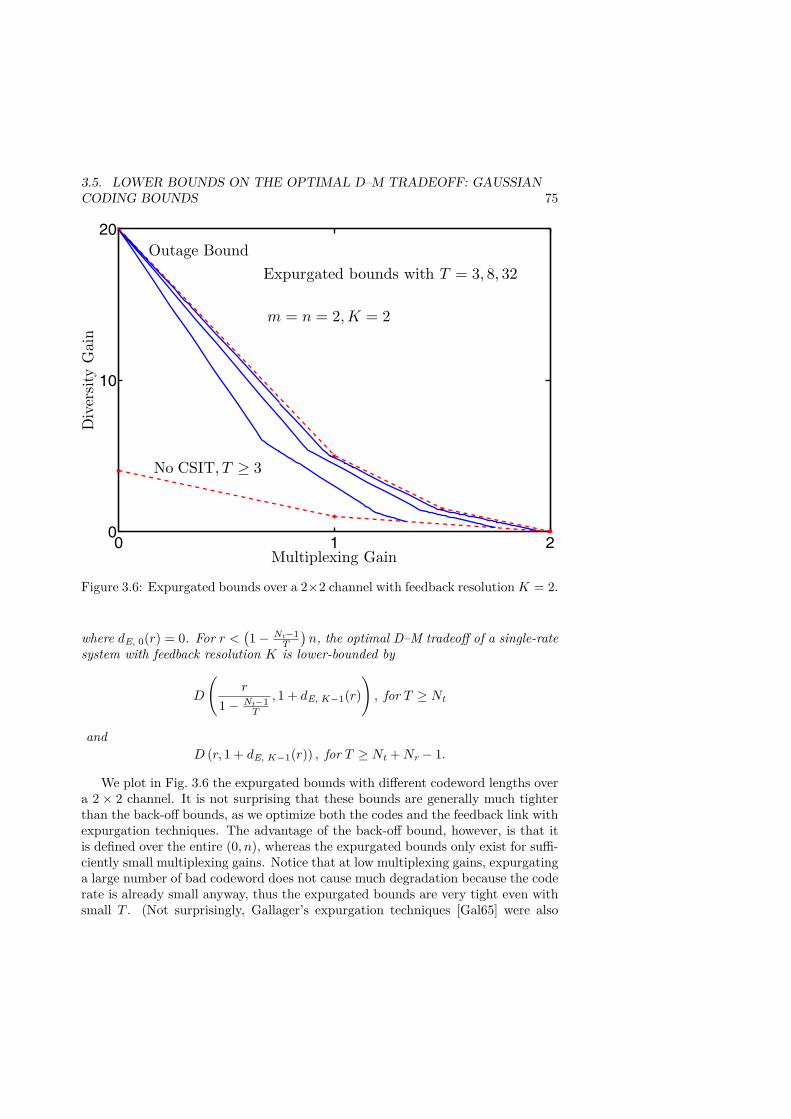
3.5. LOWER BOUNDS ON THE OPTIMAL D–M TRADEOFF: GAUSSIANCODING BOUNDS 75
0 1 20
10
20
Multiplexing Gain
Div
ersi
tyG
ain
No CSIT, T ≥ 3
Outage Bound
m = n = 2, K = 2
Expurgated bounds with T = 3, 8, 32
Figure 3.6: Expurgated bounds over a 2×2 channel with feedback resolutionK = 2.
where dE, 0(r) = 0. For r <(1− Nt−1
T
)n, the optimal D–M tradeoff of a single-rate
system with feedback resolution K is lower-bounded by
D
(r
1− Nt−1T
, 1 + dE, K−1(r)), for T ≥ Nt
andD (r, 1 + dE, K−1(r)) , for T ≥ Nt +Nr − 1.
We plot in Fig. 3.6 the expurgated bounds with different codeword lengths overa 2 × 2 channel. It is not surprising that these bounds are generally much tighterthan the back-off bounds, as we optimize both the codes and the feedback link withexpurgation techniques. The advantage of the back-off bound, however, is that itis defined over the entire (0, n), whereas the expurgated bounds only exist for suffi-ciently small multiplexing gains. Notice that at low multiplexing gains, expurgatinga large number of bad codeword does not cause much degradation because the coderate is already small anyway, thus the expurgated bounds are very tight even withsmall T . (Not surprisingly, Gallager’s expurgation techniques [Gal65] were also

76 CHAPTER 3. D–M TRADEOFF IN MIMO CHANNELS
proposed for low-rate codes.) As can be seen, for moderate codeword length T , thelower bounds quickly approach for outage bound over the entire (0, n).
The same idea can be applied for adaptive-rate transmission. For brevity, weomit the derivations and summarize the results as follows.
Proposition 3.4. For k = 2, . . . ,K − 1, define recursively
dE, k(r, rmin) = D(rmin
1− Nt−1T
, 1 + dE, k−1(r, rmin))
where dE, 1(r, rmin) = D(
r
1−Nt−1T
, 1)
, ∀rmin. For r ∈ [rmin,(1− Nt−1
T
)n), the op-
timal D–M tradeoff of an adaptive-rate system with feedback resolution K is lower-bounded by
D
(rmin
1− Nt−1T
, 1 + dE, K−1(r, rmin)), for T ≥ Nt
andD (rmin, 1 + dE, K−1(r, rmin)) , for T ≥ Nt +Nr − 1.
We plot both the back-off and expurgated bounds for adaptive transmission withNt = Nr = 2, rmin = 0.5 in Fig. 3.7. The back-off bounds consist of three sectionsconnected at r = 1− 5.5
T , 2− 2.5T if T ≥ 6, and two sections connected at r = 2− 2.5
Tfor T = 3, 4, 5. The last segment of the back-off bound can be interpreted as therange where attempts to balance the SNR exponent in the outage and outage-freeregion fail. Indeed, if r ≥ 2− 2.5
T then d∗B,2(r, 0.5) = T (2− r) and most errors occurin the outage-free region. At the multiplexing gain r = 2− 2.5
T the diversity gain isT (2 − (2 − 2.5
T )) = 2.5, for any T ≥ 3. It is interesting to observe that the right-most points of expurgated bounds also seem to have this diversity gain. This canbe explained as follows. At sufficiently high rate, expurgating results in a back-offthreshold close to n, thus the probability that I = 2 is in the order of SNR−ε forsome small ε > 0. The power P2 therefore is in the order of SNR1+ε and thus thediversity of a system with expurgated Gaussian codes is D(rmin, 1 + ε) → 2.5 asε ↓ 0.
We may draw some conservative conclusions, keeping in mind that results de-rived are only lower bounds. Unlike in the no-CSIT case [ZT03], Gaussian codingarguments do not appear to be sufficient to complete the D–M tradeoff analysis. Itis likely that many other randomly drawn codes also suffer from this phenomenonand therefore are not immediately suitable for the feedback model considered herein.Nevertheless, such a random code with moderate codeword lengths and/or carefulexpurgation may quickly approach outage bounds, when combined with a properlydesigned feedback scheme.

3.6. CONCLUSION 77
0.5 1 1.5 20
5
10
12.5
Multiplexing Gain
Div
ersi
tyG
ain
Outage Bound
No CSIT, T ≥ 3
m = n = 2, K = 2, rmin = 0.5
Bounds with T = 3, 8, 32
Solid: Back-offDashed: Expurgated
Figure 3.7: Gaussian coding bounds for adaptive-rate transmission over a 2 × 2channel with feedback resolution K = 2, rmin = 0.5.
3.6 Conclusion
In this chapter, we have analyzed the asymptotic behavior of MIMO systems withslow fading and quantized CSIT under the framework of the D–M tradeoff. Whilethis is clear that an error event is very unlikely in such a high-SNR scenario, wehave been able to characterize exactly the level of unlikelihood of that event. Wehave shown that, unlike in the no-CSIT case, even carefully constructed feedbackschemes with Gaussian codes are not sufficient to complete the achievability partof the optimal D–M tradeoff. Instead, the optimal D–M tradeoff is shown to beachievable by combining a certain class of finite-length codes with a suitable feed-back scheme. Our extended approximately universal condition gives some novelinsight into the class of codes that are D–M tradeoff optimal over any channel dis-tribution. Altogether, the results provide a better understanding on the behaviorof adaptive MIMO systems in the asymptotically high SNR regime.

78 CHAPTER 3. D–M TRADEOFF IN MIMO CHANNELS
Appendices for Chapter 3
3.A Proof of Lemma 3.1
We first show that the optimal index mapping must have the form (3.12). Noticethat for an optimal scheme, the power constraint is active, because the joint p.d.f.of the singular values of the channel matrix are continuous and takes on positivevalues over the entire positive orthant.
Let {Pi}Ki=1 be an arbitrary power codebook and I(H) be a deterministic indexmapping such that 0 ≤ P1 < . . . < PK and
∑Ki=1 Pr(I(H) = i)Pi ≤ SNR. Consider
another feedback scheme using the same power codebook and the following indexmapping
I(H) Δ={
1 if I(H, PI(H)) < R,min{i : i ∈ {1, . . . , I(H)}, I(H, Pi) ≥ R} otherwise.
This gives exactly the same outage probability as I(H) does. However, by con-struction, the average transmit power of the newly constructed scheme is
K∑i=1
Pr(I(H) = i)Pi ≤K∑i=1
Pr(I(H) = i)Pi.
This means that we can restrict our attention to I(H) with the following properties.Firstly, all channel realizations that are in outage are mapped to I = 1. Secondly,a channel realization H, if not in outage, is mapped to the smallest power in thepower codebook that can “invert” H, i.e., when this power level is applied at thetransmitter, the mutual information is greater than R.
It remains to show that no set of channel realizations with strictly positiveprobability measure that can be inverted by some Pi, i ≥ 2, is mapped to I = 1.Assume the contrary, i.e., there exists a set S and an index j ≥ 2 such thatPr(H ∈ S) = πS > 0 and I(H, Pj) ≥ R, I(H) = 1, ∀H ∈ S. Then there ex-ists a Pj ∈ (Pj−1, Pj) such that Pr
(Pm(H;Rj) ∈ (Pj , Pj)
)= πS where Pm(H;R)
satisfies I (H, Pm(H;R)) = R, i.e., the minimum power required to invert thechannel matrix H. Since all choices of S subject to Pr(H ∈ S) = πS are equiv-alent in terms of both average power and outage probability, we can considerS =
{H : Pm(H;R) ∈ (Pj , Pj)
}.
Now consider another feedback scheme using the index mapping I(H) and thepower codebook {P1, . . . , Pj−1, Pj , Pj+1, . . . , PK}. By construction, this gives thesame outage probability as that obtained by the codebook {Pi}Ki=1 together withI(H). However the newly constructed scheme uses less average power, becausePj < Pj , i.e. the power constraint is inactive. Thus, the optimal index mappingmust have the form (3.12), which yields an outage probability of F (R,P ∗K).

3.B. PROOF OF THEOREM 3.1 79
Finally, because P ∗1 < · · · < P ∗K , the event I(P ∗i−1,H) > R also impliesI(P ∗i ,H) > R. Thus
Pr(I(P ∗i ,H) > R, I(P ∗i−1,H) < R
)= Pr
(I(P ∗i−1,H) < R
)− Pr (I(P ∗i ,H) < R)= F
(R,P ∗i−1
)− F (R,P ∗i ) .
Therefore the average power of the system is given by
[F (R,P ∗K) + 1− F (R,P ∗1 )]P ∗1 +K∑i=2
[F (R,P ∗i−1)− F (R,P ∗i )]P ∗i .
Since F (R,PK) is a monotonically decreasing function of PK for any given R > 0,the optimal power codebook is the solution to (3.11).
3.B Proof of Theorem 3.1
First we derive an upper bound on the SNR exponent of the largest power level inthe optimal power codebook, i.e., P ∗K . Let {P i} be the solution to the followingoptimization problem, which is a relaxed version of (3.11),
max PK
s.t. [F (R,PK) + 1− F (R,P1)]P1 ≤ SNR,[F (R,Pi−1)− F (R,Pi)]Pi ≤ SNR, i ≥ 2,0 ≤ P1 < · · · < PK .
(3.25)
Clearly PK ≥ P ∗K due to relaxation. Note that the constraints of (3.25) imply∑Ki=1
SNRP i≥ 1. We must have P 1 ≤ KSNR otherwise
∑Ki=1
SNRP i< K 1
K = 1.Because K is a finite constant, we have P 1 ≤ SNR. An application of Lemma 3.2leads to F (R,P 1) ≥ SNR−D(r,1) = SNR−d
∗out, 1(r).
The constraints of (3.25) also require SNRP 2
+ F (R,P 2) ≥ F (R,P 1), leading to
SNRP 2
+ F (P 2) ≥ SNR−d∗out, 1(r). (3.26)
For any ε > 0, if P 2.= SNR1+d∗out, 1(r)+ε then
SNRP 2
+ F (P 2) .= SNR−d∗out, 1(r)−ε + SNR−D(r,1+d∗out, 1(r)+ε),
which contradicts to (3.26) because D(r, 1 + d∗out, 1(r) + ε) > D(r, 1) = d∗out, 1(r).Therefore we must have P 2 ≤ SNR1+d∗out, 1(r), and thus
F (R,P 2) ≥ SNR−D(r,1+d∗out, 1(r)) = SNR−d∗out, 2(r).

80 CHAPTER 3. D–M TRADEOFF IN MIMO CHANNELS
By induction, we eventually obtain PK ≤ SNR1+d∗out, K−1(r) and
F (R,P ∗K) ≥ F (R,PK) ≥ SNR−D(r,1+d∗out, K−1(r)) = SNR−d∗out, K(r).
Finally, a lower bound on P ∗K is obtained by choosing P 1 = SNRK , P 2 = SNR
KF (P 1) ,. . ., PK = SNR
KF (PK−1) . Since these P i’s satisfy the constraints of (3.11), we haveP ∗K ≥ PK . Because K is a finite constant and by construction, P 1
.= SNR, P 2.=
SNR1+d∗out, 1(r), . . ., PK.= SNR1+d∗out, K−1(r). Thus
F (R,P ∗K) ≤ F (R,PK) .= SNR−d∗out, K(r).
This concludes the proof.
3.C Proof of Theorem 3.2
Similarly to the single-rate case, Qi = PiNt
INt , ∀i ∈ {1, . . . ,K}, can be assumedwithout loss of generality.
Consider an arbitrary sequence of deterministic feedback schemes F that pro-vides a multiplexing gain of r. Let the outage probability Pout,F
.= SNR−dout,F (r).We now derive an upper bound on dout,F (r). To that end, let pi, i = 1, . . . ,K, bepositive real numbers such that Pi
.= SNRpi . From (3.3), we have
K∑i=1
Pr(I = i)SNRpi ≤ SNR. (3.27)
Without loss of generality, assume that 0 < p1 ≤ · · · ≤ pK . Let K be the integerin {1, . . . ,K} such that pK ≤ 1 and pK+1 > 1. Herein we use the conventionpK+1 = ∞. Such a K must exist, otherwise (3.27) cannot be satisfied. Note that(3.27) implies Pr(I = i)SNRpi ≤ SNR, ∀i. Thus Pr(I = i) ≤ SNR1−pi , and
limSNR→∞
Pr(I = i)Rilog SNR = ri lim
SNR→∞Pr(I = i) = 0,∀i ≥ K + 1,
meaning that all regions using a power whose SNR exponent is strictly larger than1, if any, contribute nothing to the multiplexing gain (3.5). In our context, K canbe interpreted as the number of regions that contribute considerably to the overallthroughput, while K − K can be seen as the number of regions that are added toimprove the overall reliability.
Consider the first K regions of F , with power levels having dominant SNRexponent less than or equal to 1, and let rmax = max(r1, . . . , rK). By defini-tion (3.5), r ≤ rmax. Let us consider another sequence of feedback schemes Fusing r1 = r < rmax, ri = rmin ≤ ri, ∀i ≥ 2 and having P1
.= SNR. LetPout,F
.= SNR−dF (r). Outage probability is an increasing function of rate and de-creasing function of power, thus maximizing dF (r) yields an upper bound to dF (r).

3.C. PROOF OF THEOREM 3.2 81
If a multiplexing gain of r is achievable even with an outage-minimizing F , thenthe lower bound is tight.
We claim that to minimize the SNR exponent of outage, it suffices to considerF such that
pi > 1, ∀i ≥ 2 (3.28)where Pi
.= SNRpi . Assume the contrary, then at least P2.= SNR. Then dF (r) can
be upper-bounded by d∗K−1(rmin), i.e., the outage exponent of a single-rate systemwith rate rmin log SNR and a coarser resolution of K − 1. It is easy to show thatsuch an upper bound is strictly below the achievable dF (r) when assuming (3.28),derived below.
Assume (3.28) holds, i.e., K = 1. For sufficiently high SNR, (3.28) impliesP1 < Pi, ∀i > 2. We can characterize the optimal index mapping and powercodebook with the following lemma, which is a straightforward generalization ofLemma 3.2.
Lemma 3.3. Consider a system employing some given rates R1 > R2 = · · · = RK .It is constrained that 0 ≤ P1 < · · · < PK . The outage-minimizing power codebook{P ∗i }Ki=1 solves
max PK
s.t. [F (RK , PK) + 1− F (R1, P1)]P1 +K∑i=2
[F (Ri−1, Pi−1)− F (Ri, Pi)]Pi ≤ SNR.
(3.29)
The optimal index mapping is given by
I∗(H) ={
1 if I(H, P ∗K) < RK ,min{i : i ∈ {1, . . . ,K}, I(H, P ∗i ) ≥ Ri} otherwise.
(3.30)
The minimum outage probability is
P ∗out = F (RK , P ∗K).
The proof is almost identical to that of Lemma 3.2 and therefore omitted forbrevity. Similarly to Appendix 3.B, computing the SNR exponent of P ∗K thatsolves (3.29) gives the optimal d∗F (r) = d∗out,K(r, rmin).
Recall that d∗F (r) is only an upper bound on dF (r) because the multiplexinggain of F may actually be smaller than r due to construction. To show the tightnessof the bound, consider the following power levels for F
P 1 = SNRK,P 2 = SNR
KF (R1, P 1) , . . . , PK = SNRKF (RK−1, PK−1) ,
which satisfy (3.28), and also achieve d∗F (r). It is not difficult to verify that
limSNR→∞
Pr(I = 1) = limSNR→∞
[F (RK , PK) + 1− F (R1, P 1)] = 1,

82 CHAPTER 3. D–M TRADEOFF IN MIMO CHANNELS
and limSNR→∞ Pr(I = i) = 0, ∀i > 1. By definition (3.5), the multiplexing gain ofsuch a scheme is exactly r.
3.D Towards the Necessity of (3.18)
In this section, we will show that, if a sequence of codes C satisfies
lim infSNR→∞
(minC
∏nj=1 SNR−(βj)+
)log SNR = −r (3.31)
for some r > r, then for a certain sequence of channel distributions, there existchannels in the ε-outage-free region that make the maximum pairwise error prob-ability bounded away from zero even as SNR → ∞. Furthermore, the probabilitymeasure of such bad channels set decays only polynomially with SNR.
To that end, considerOε = {H : I(H,SNR) ≥ (r + ε) log SNR}.
If the condition (3.31) holds, then for arbitrarily small δ > 0, we can find SNR sothat for any SNR > SNR, there exists a codeword differences ΔXB with squaredsingular values μj = SNR−βj such that
∑nj=1(βj)+ ≥ r − δ. For sufficiently small
δ, then r − δ > r > 0, thus at least β1 > 0.Choose a sequence of distributions that always align the singular values λj
of the channel matrix to those of ΔXB in the worst order, i.e., ‖HΔXB‖2F =∑nj=1 λjμn+j−1, ∀H. For convenience, also choose λn1 to be Wishart distributed
(which can be made independent of the choice of the worst-case rotation). Then
maxC
Pr(pairwise error,H ∈ Oε)≥ Pr(pairwise error,ΔXB,H ∈ Oε)
=∫OεQ
⎛⎝√√√√SNR
2Nt
n∑j=1λjμn−j+1
⎞⎠ f(λn1 )dλn1
≥ 12√π
∫Oε
exp(−SNR
4Nt
∑nj=1 λjμn−j+1
)1 +√
SNR2Nt
∑nj=1 λjμn−j+1
f(λn1 )dλn1
.=∫Oε
1
1 +√∑n
j=1 SNR1−αj−βn−j+1exp
⎛⎝− n∑
j=1SNR1−αj−βn−j+1
⎞⎠ f(λn1 )dλn1
.=∫Bf(αn1 )dαn1 + SNR−∞
where the second inequality is due to the fact that
Q(x) ≥ 12√π
exp(−x2/2)1 + x , ∀x ≥ 0.

3.D. TOWARDS THE NECESSITY OF (3.18) 83
The bad channels set B where the pairwise error probability is in the order of SNR0
is given as
B = {αn1 : α1 ≥ · · · ≥ αn ≥ 0} ∩ {αn1 : 1− αj < βn−j+1}
∩⎧⎨⎩αn1 :
n∑j=1
(1− αj)+ ≥ r + ε
⎫⎬⎭ .
Let r = min (1, r − δ). Since β1 > 0 ∀SNR > SNR, the function∑nj=1(1− αj)+ is
continuous and assumes all values on [0, r) for the αn1 ’s in the intersection of thefirst two sets defining B. Thus for any r ∈ (0, r), B can be made nonempty bychoosing, e.g.,
ε = r − r2 .
With that choice of r and ε, over B, the function∑nj=1(2j−1+m−n)αj is continuous
and bounded below, and Varadhan’s integral lemma [DZ98] can be applied to showthat the probability that H ∈ B is dominated by the term
SNR− infB∑n
j=1(2j−1+m−n)αj
as SNR→∞. Thus there exists a set of “bad” channels in the ε-outage-free regionthat make the largest pairwise error probability in the order of SNR0 (boundedbelow by a positive constant). Furthermore the probability measure of that setdoes not decay exponentially. This makes the largest pairwise error probabilityaveraged over Oε decay sub-exponentially.


Chapter 4
D–M Tradeoff inDecode–and–Forward RelayChannels
This chapter studies the problem of resource allocation to maximize the outage ex-ponent over a decode-and-forward fading relay channel with quantized channel statefeedback (CSF). Three different scenarios are considered: relay-source, destination-relay, and destination-source CSF. It is found that using just one bit of CSF fromthe relay to control the source transmit power is sufficient to achieve the multi-antenna upper bound in a range of multiplexing gains, with fixed-length codes, i.e.,with coding schemes significantly simpler than dynamic DF. Systems with CSFfrom destination to control relay transmit power slightly outperform DDF at highmultiplexing gains, even with one bit of feedback. Finally, with CSF from destina-tion, if the source-relay channel gain is unknown to the feedback quantizer at thedestination, the diversity gain only grows linearly in the number of feedback levelsK, in sharp contrast to an exponential growth for multiantenna channels. In thislast scenario, a simple scheme is shown to perform close to the corresponding upperbound.
4.1 Introduction
Motivated by the potential of having simple single-antenna communication nodescooperate and approach the promising performance of multiantenna systems, therehas been a renewed interest in the classical relay channels [van71, CE79], for ex-ample in the recent work [SEA03a, SEA03b, LW03, LTW04, NBK04, KGG05].Resource allocation for relay channels is known to enhance the performance sig-nificantly in many different scenarios [HA04, MY04, LC05, GE07a, HZ05, LV05,LVP07]. Most previous work on resource allocation, however, assumed perfect net-work state information at both the source and the relay. In [AKSA06], power
85

86CHAPTER 4. D–M TRADEOFF IN DECODE–AND–FORWARD RELAY
CHANNELS
control for AF relaying with quantized feedback from the destination is considered,but a diversity analysis is not pursued.
For the relay channel, the D–M tradeoff curves of some baseline schemes areobtained in [LTW04, PV04]. A sophisticated scheme named dynamic decode-and-forward is proposed in [AES05] and shown to achieve the multi-antenna upperbound at all multiplexing gains less than one-half. The D–M tradeoff over AFrelay channels is extensively treated in [AES05, YB07a, YB07b]. From a diversity-multiplexing tradeoff viewpoint, CF relaying is shown to be optimal [YE07], un-der the critical assumption that the relay knows the full CSI. In the recent work[EVAK06], optimizing the dimension allocation for DF using only the statisticalknowledge of the channel is considered.
This chapter considers a three-node half-duplex cooperative communicationchannel subject to very slowly-varying, but random, channel gains (quasi-staticfading), under different forms of heavily quantized CSF. The partial CSF is usedto allocate the number of channel uses in the two phases of the DF protocol, i.e.,dimension allocation, and also to control the transmit power across fading states.Both orthogonal (source and relay do not transmit simultaneously) and nonorthog-onal (source and relay can transmit at the same time) schemes are considered.
Three different feedback scenarios are considered: relay-to-source CSF, destination-to-source-and-relay CSF, and destination-to-relay CSF. The last case is motivatedby the fact that in certain scenarios, the feedback link from the destination to thesource is of significantly lower quality than that from the destination to the relay(which inspires the relaying model in the first place). The possibilities that we donot study are the destination-to-source CSF case and the scenario of joint feedbackfrom both the relay and the destination. The former case is omitted because of therelative distances between the nodes in practice. It is unrealistic that the feedbackfrom the destination is reliably received by the source but not by the relay, due tothe broadcast nature of wireless communications. As for the latter case, we choseto study only separate feedback from either the relay or the destination to simplifythe analysis and also to get insight into the actual value of each individual feedbacktype.
As in Chapter 3, we study the asymptotically high SNR regime in terms ofthe D–M tradeoff. A summary of our findings in this chapter is given in the fol-lowing. Over a statistically symmetric Gaussian decode-and-forward relay channel(the channel is described more precisely later) with
Relay-to-source CSF:
• With dimension allocation only, performance gains over no-CSF schemes canbe achieved even with heavily quantized CSF from the relay to the source.Nonorthogonal schemes provide additional, but not very significant gainsover an orthogonal system.
• With dimension allocation and power control at the source, even one bit ofCSF is sufficient to achieve the fully cooperative upper bound over a widerange of multiplexing gains.

4.2. SYSTEM MODEL 87
• Relay-to-source CSF systems quickly approach the performance of DDF[AES05] as the quality of CSF increases. Our results suggest the use ofan orthogonal DF scheme with as few as one bit of CSF from the relay, incombination with power control at the source.
Destination-to-relay CSF: Our proposed nonorthogonal scheme with powercontrol at the relay slightly outperforms DDF for large values of multiplexing gain.Furthermore, the performance of one bit CSF and perfect CSF is virtually indistin-guishable. The results first imply that with perfect CSF, this DF and power controlscheme is much less efficient than a compress-and-forward approach [YE07]. Sec-ond, with limited CSF, our results suggest the use of just one bit to control relaytransmit power for high-rate DF systems.
Destination-to-source-and-relay CSF:• By developing a novel upper bound to the diversity gain for channels with
restricted CSF (see Section 4.6), we show that under the relatively realis-tic assumption that the source-relay channel gain is unknown to the feed-back quantizer at the destination, the diversity gain only grows linearly inthe number of feedback levels (also referred to as feedback resolution). Incontrast, the diversity gain of a MISO channel grows exponentially in thefeedback resolution K.
• A proposed scheme is shown to perform relatively close to the new upperbound.
The results above are obtained in the limit of infinitely large block lengths. Wethen discuss the achievable tradeoffs with finite-length codes, arguing that in theorthogonal case, “good” codes designed for parallel channels are also suitable forthe DF relay scenario. Inspired by the concept of approximate universality [TV06]we next present sufficient conditions for finite-length codes to achieve the optimalexponent. By expurgating codes drawn from Gaussian ensemble to match thenew sufficient conditions, we show the existence of codes that approach the outageexponent for all multiplexing gains even at moderate block lengths. In this scenario,the loss in performance of finite block length schemes comes from the discretenessof the possible dimension allocation ratios, rather than from the length of the codes.
4.2 System Model
Consider the complex baseband model of a frequency-nonselective fading relay chan-nel in Fig. 4.1. The channel is assumed to be slowly fading, i.e., the channel gainsare constant during a fading block consisting of T channel uses, but changes in-dependently from one block to the next. We exclusively consider the case when atransmission codeword spans a single fading block to identify the gain of spatialcooperation. The channel is assumed to be statistically symmetric. In particular,the channel gains between source-destination, source-relay and relay-destination h,h1, and h2 are i.i.d. complex Gaussian random variables with zero mean and unitvariance. Let g = |h|2, γ1 = |h1|2 and γ2 = |h2|2. Assume perfect channel state

88CHAPTER 4. D–M TRADEOFF IN DECODE–AND–FORWARD RELAY
CHANNELS
s1 s2
sR
w1 w2
wR
y1 y2
yR
hh
h1 h2
¯T (1¡ ¯)T
Figure 4.1: System model.
information at the receiver of each communication link. We also assume perfectsynchronization.
We consider a half-duplex channel, where the relay cannot transmit and receivesimultaneously. Communication between source and destination takes place in twophases. In the learning phase, the source transmits, the relay and the destinationlisten. In the relaying phase the relay transmits based on what it has learnedand the source may transmit more symbols but no new message (in nonorthogonalschemes), or remain silent (in orthogonal schemes). The destination attempts todecode based on the entire signals received during both phases.
The received signals at time instant n during the learning phase are given by
y1(n) = hs1(n) + w1(n)yR(n) = h1s1(n) + wR(n).
(4.1)
In the relaying phase, the received signal at the destination is
y2(n) = hs2(n) + h2sR(n) + w2(n) (4.2)
where for an orthogonal scheme s2 = 0 (this will be discussed in more detail lateron). The noises w1, w2, wR are mutually independent temporally white complexGaussian with zero mean and unit variance.
Assume individual power constraints at the source and the relay. We considerboth short-term and long-term power constraints [CTB99], which are specified inmore detail later. We will also refer to systems under a short-term (respectivelylong-term) power constraint as ones without power control (respectively, with powercontrol).
At each value of SNR, the system is designed to serve a fixed rate of r log SNRbits per channel use (which is independent of the CSI at the transmitter), where

4.3. DECODE-AND-FORWARD WITHOUT CSF 89
r ∈ (0, 1) is the multiplexing gain. That is, no rate control is possible. Assume thatall three links in the model have the same SNR. This is not too restrictive because,as long as the SNR’s of the three links scale in the same order, the diversity–multiplexing tradeoff does not change. Recall from Chapter 3 that the system hasa diversity gain of d if the probability of error at the destination satisfies
Pr(ε) .= SNR−d.
We are interested in characterizing d as a function of r for different feedback schemesover the channel. In Sections 4.3-4.6, we focus on the SNR exponent of the outageprobability Pout(r log SNR), also referred to as the outage exponent. Herein outageis defined as the event that the relevant instantaneous mutual information (givena particular scheme) is smaller than the data rate r log SNR. One should exercisesome extra care when interpreting the meaning of the outage exponents in the cur-rent work. The outage exponents discussed herein do not serve as a universal upperbound to the diversity-multiplexing tradeoff as in the multi-antenna case, as findingthe capacity of the general relay channel is a long-standing open problem.1 Rather,they represent the achievable tradeoffs of specific schemes. We can achieve thesetradeoffs by using standard Gaussian coding arguments, first letting the codewordlength T → ∞ for each SNR and then considering a sequence of schemes with in-creasing SNR. Achievability results with finite-length codes will be presented anddiscussed later in Section 4.7.
4.3 Decode-and-Forward without CSF
When the source and relay have no information about their corresponding instan-taneous forward channel gains, the system can still optimize the SNR exponent ofthe outage probability using the knowledge about the statistics of the channel.
This optimization for DF with multiple relays has been solved in [EVAK06]. Wesummarize the results herein along with a sketch of the proof in order to introducesome important concepts and help facilitate the presentation of more sophisticatedCSF schemes. In addition, we will later present novel results on finite-length codesin Section 4.7, and show that this practical constraint changes the picture consid-erably.
In this simple setting, the learning phase uses T1 = βT channel uses and therelaying phase uses T2 = (1 − β)T channel uses where 0 < β < 1 is the fractionof dimension allocated that we want to optimize over. The source encodes anequally likely message m ∈ {1, . . . , 2rT log SNR} to a sequence {s1(1), . . . , s1(T1),s2(1), . . . , s2(T2)} belonging to a codebook C1 where s2(1) = · · · = s2(T2) = 0 for
1With an exception for the cooperative bounds, which are universal upper bounds for anypossible relaying scheme.
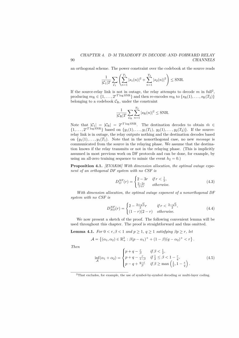
90CHAPTER 4. D–M TRADEOFF IN DECODE–AND–FORWARD RELAY
CHANNELS
an orthogonal scheme. The power constraint over the codebook at the source reads
1|C1|T
∑C1
(T1∑n=1|s1(n)|2 +
T2∑n=1|s2(n)|2
)≤ SNR.
If the source-relay link is not in outage, the relay attempts to decode m in full2,producingmR ∈ {1, . . . , 2rT log SNR} and then re-encodesmR to {sR(1), . . . , sR(T2)}belonging to a codebook CR, under the constraint
1|CR|T
∑CR
T2∑n=1|sR(n)|2 ≤ SNR.
Note that |C1| = |CR| = 2rT log SNR. The destination decodes to obtain m ∈{1, . . . , 2rT log SNR} based on {y1(1), . . . , y1(T1), y2(1), . . . , y2(T2)}. If the source-relay link is in outage, the relay outputs nothing and the destination decodes basedon {y1(1), . . . , y1(T1). Note that in the nonorthogonal case, no new message iscommunicated from the source in the relaying phase. We assume that the destina-tion knows if the relay transmits or not in the relaying phase. (This is implicitlyassumed in most previous work on DF protocols and can be done, for example, byusing an all-zero training sequence to mimic the event h2 = 0.)
Proposition 4.1. [EVAK06] With dimension allocation, the optimal outage expo-nent of an orthogonal DF system with no CSF is
DNFO (r) =
{2− 3r if r < 1
3 ,2−2r1+r otherwise.
(4.3)
With dimension allocation, the optimal outage exponent of a nonorthogonal DFsystem with no CSF is
DNFNO(r) =
{2− 3+
√5
2 r if r < 3−√52 ,
(1− r)(2− r) otherwise.(4.4)
We now present a sketch of the proof. The following convenient lemma will beused throughout this chapter. The proof is straightforward and thus omitted.
Lemma 4.1. For 0 < r, β < 1 and p ≥ 1, q ≥ 1 satisfying βp ≥ r, let
A ={
(α1, α2) ∈ R2+ : β(p− α1)+ + (1− β)(q − α2)+ < r
}.
Then
infA
(α1 + α2) =
⎧⎪⎪⎨⎪⎪⎩p+ q − rβ if β < 1
2 ,
p+ q − r1−β if 1
2 ≤ β < 1− rq ,p− q + q−r
β if β ≥ max(
12 , 1− rq
).
(4.5)
2That excludes, for example, the use of symbol-by-symbol decoding or multi-layer coding.

4.3. DECODE-AND-FORWARD WITHOUT CSF 91
We now briefly present the proof for the orthogonal part of Proposition 4.1 (thenonorthogonal case can be proved similarly). The event that the relay is in outageand the source-destination link is in outage is given by
O1 = {(β log(1 + SNRγ1) < r log SNR) ∩ (β log(1 + SNRg) < r log SNR)} .
The event that the relay is not in outage, but the effective channel from source todestination is still in outage is given by
O2 = {(β log(1 + SNRγ1) ≥ r log SNR)∩ (β log(1 + SNRg) + (1− β) log(1 + SNRγ2) < r log SNR)} .
The overall outage probability is thus
Pout = Pr(O1 ∪ O2) = Pr(O1) + Pr(O2)
since O1 and O2 are mutually exclusive. The outage exponent is
Pout(r log SNR) .= SNR−D1 + SNR−D2 (4.6)
where D1 and D2 are the SNR exponents of O1 and O2 respectively.Let us perform the standard change of variables αi = − log γi/ log SNR and
a = − log g/ log SNR [ZT03, AES05]. Then, the set of channel realizations corre-sponding to O1 is
A1 ={
(α1, α2, a) ∈ R3+ : (1− α1)+ <
r
β, (1− a)+ <
r
β
}
and
D1 = infA1
(α1 + α2 + a) =(
2− 2rβ
)+
.
For an optimal system, the condition r ≤ β must be satisfied otherwise D1 = 0,i.e., the outage probability will not decay to zero as the SNR increases. Thus fromnow on, we constrain β ≥ r.
Consider the second SNR exponent D2 = infA2(α1 + α2 + a) where
A2 = {(α1, α2, a) ∈ R3+ : β(1− α1)+ ≥ r, β(1− a)+ + (1− β)(1− α2)+ < r}.
The event β(1−α1)+ ≥ r has a probability in the order of SNR0 and is independentof the event β(1 − a)+ + (1 − β)(1 − α2)+ < r. Thus by invoking Lemma 4.1, weobtain
D2 =
⎧⎪⎨⎪⎩
2− rβ if r < β < 12 ,
1−rβ if r ∈ (1− β, β), β ≥ 1
2 ,
2− r1−β if r < 1− β, β ≥ 1
2 .
(4.7)

92CHAPTER 4. D–M TRADEOFF IN DECODE–AND–FORWARD RELAY
CHANNELS
The slowest decayed term on the right hand side of (4.6) is the dominatingone as SNR → ∞, thus we have Dout(r) = min(D1,D2). The outage exponentcorresponding to an optimal dimension allocation is given by
DNFO (r) = sup
β∈[r,1)min(D1,D2).
Due to the symmetry of D2, for a given r ≤ 1/2 and any β ∈ (r, 1/2] there existsa β = (1 − β) ∈ [1/2, 1 − r) that results in D2 = D2. But β ≥ β thus D1 ≤ D1and min(D1,D2) ≤ min(D1, D2). This means there is no loss of optimality byconsidering β ≥ 1/2 and
DNFO (r) = sup
β∈[max(r,1/2),1)min(D1,D2).
The results then follow a straightforward investigation.Both the fixed DF schemes with no CSF in Proposition 4.1 are unsurprisingly
outperformed by the DDF scheme [AES05] for any r ∈ (0, 1). Recall that in theDDF scheme, the source keeps transmitting until the accumulated mutual infor-mation at the relay is sufficient for decoding (the relay informs the source aboutsuch an event by an acknowledgement bit). Therefore DDF requires rateless codes,which are more complicated than codes with fixed lengths needed for the fixed DFapproaches. We will further improve the simple fixed DF schemes with the help ofquantized channel state information in the next sections.
4.4 Relay-to-Source CSF
In this section, we assume that given the channel h1, the relay sends an indexI(h1) ∈ {1, . . . ,K} back to the source via an error-free zero-delay feedback link.The positive integer K is referred to as the resolution of the feedback link. Thesource allocates dimension (under a short-term power constraint) and both dimen-sion and power (under a long-term power constraint). Since the two channel gainsto the destination are unknown at the source and relay, the outage exponent of thisscheme can be upper-bounded by that of a MISO 2× 1 channel with no-CSIT (i.e.,the fully cooperative transmitters bound), DMISO(r) = 2− 2r.
Short-term Power ConstraintFirst consider a short-term power constraint case, i.e., no power control at thesource. Let βk be the fraction of dimension allocated for the learning phase givenfeedback index k, β1 < β2 < · · · < βK . Recall that the information rate r log SNRis independent of the feedback index. Consider the index mapping
I(γ1) ={K if βK log(1 + γ1SNR) < r log SNR,min {k ∈ {1, . . . ,K} : βk log(1 + γ1SNR) ≥ r log SNR} otherwise.

4.4. RELAY-TO-SOURCE CSF 93
That is, from a finite set of {βk} the source allocates the minimum dimension so thatthe rate can be supported by the source-relay link. If the rate is not supportableeven with the largest dimension βK , then the index I = K is fed back so that thedirect link can benefit the most in the orthogonal case (in the nonorthogonal case,whatever index sent back when the relay fails does not matter because the directtransmission always uses all the available dimension).
We quantify the outage exponent of the scheme described above in the followingproposition. The proof is deferred to Appendix 4.A.
Proposition 4.2. An orthogonal scheme without power control and with relay-to-source CSF resolution K can achieve an outage exponent of
DRF−KO-NPC(r) = sup
max(r,0.5)≤β1<···<βK<1min(D1, . . . , DK , 2
(1− rβK
))(4.8)
where
Dk ={
3− r1−βk − r
βk−1if βk < 1− r,
1−rβk
+ 1− rβk−1
otherwise,(4.9)
with the convention β0 = r.A nonorthogonal scheme without power control and relay-to-source CSF resolu-
tion K can achieve an outage exponent of
DRF−KNO-NPC(r) = sup
max(r,0.5)≤β1<···<βK<1min(D1, . . . , DK , 2− r − r
βK
)(4.10)
where Dk is defined as in (4.9).
Notice that for r ≥ 1/2, then Dk = 1−rβk
+ 1 − rβk−1
, ∀k, due to the constraintβk ≥ max(r, 0.5). But in general, the Dk’s in (4.9) are neither concave or convex,making the evaluation of the maximin difficult. We next present tight upper boundsand lower bounds to the optimized outage exponent in Proposition 4.2, which aresimpler to compute. The proof is in Appendix 4.B.
Proposition 4.3. The outage exponent DRF−KO-NPC(r) is lower-bounded by
DRF−KLB-O-NPC(r) =
⎧⎨⎩
2(1−r)−2(1−r)( r1−r )K
1−2r( r1−r )K
if r �= 1/22K
1+2K if r = 1/2.(4.11)
For r ≥ 1/2, we have DRF−KO-NPC(r) = DRF−K
LB-O-NPC(r).For r < 1/2, DRF−K
O-NPC(r) is upper-bounded by
DRF−KUB-O-NPC(r) = sup
1/2≤β1<···<βK<1min(D1, . . . , DK , 2
(1− rβK
))(4.12)

94CHAPTER 4. D–M TRADEOFF IN DECODE–AND–FORWARD RELAY
CHANNELS
where
Dk ={
3− r1−βk − r
βk−1if βk < 1− r,
3− r − βk − rβk−1
otherwise,(4.13)
with the convention β0 = r;The outage exponent DRF−K
NO-NPC(r) is lower-bounded by
DRF−KLB-NO-NPC(r) =
⎧⎨⎩
2(1−r)2−(1−r)( r1−r )K
1−r−r( r1−r )K
if r �= 1/21+2K2+2K if r = 1/2.
(4.14)
For r ≥ 1/2, we have DRF−KNO-NPC(r) = DRF−K
LB-NO-NPC(r).For r < 1/2, DRF−K
NO-NPC(r) is upper-bounded by
DRF−KUB-NO-NPC(r) = sup
1/2≤β1<···<βK<1min(D1, . . . , DK , 2− r − r
bK
)(4.15)
where Dk is defined in (4.13).
The lower bounds, which coincide with the actual outage exponents for r ≥ 1/2,are explicitly given. As for the upper bounds, which are only necessary whenr < 1/2, we consider all possible cases
βK1 ∈ [1/2, 1− r)× · · · × [1/2, 1− r)︸ ︷︷ ︸l times
× [1− r, 1)× · · · × [1− r, 1)︸ ︷︷ ︸K−l times
,
for l = 0, . . . ,K where A × B denotes the Cartesian product. Due to the con-straint β1 < · · · < βK , we only need to consider K + 1 such regions (and not2K). Over each of the K + 1 regions we can efficiently solve for the optimumusing convex optimization methods. The problem is convex because over either{βk−1, βk} ∈ [1/2, 1)× [1/2, 1− r) or {βk−1, βk} ∈ [1/2, 1)× [1− r, 1), the functionDk in (4.13) is concave; and the point-wise minimum of a family of concave functionis concave [BV04]. Finally, the maximum of the K + 1 solutions gives the desiredupper bound.
We plot in Fig. 4.2 the upper and lower bounds in Proposition 4.3 for orthogonalschemes. A relatively large improvement over the no-CSF case can be achieved, butthis gain diminishes as K increases from 2 to 3. As can be seen, the proposed CSFscheme is outperformed by DDF, but gradually approaches the performance of DDFas the CSF quality improves. We formalize this observation in the following.
Corollary 4.1. We have
limK→∞
DRF−KO-NPC(r) = lim
K→∞DRF−K
NO-NPC(r) ={
2− 2r if r < 12
1−rr if r ≥ 1
2 .(4.16)

4.4. RELAY-TO-SOURCE CSF 95
0 0.5 10
1
2
Multiplexing Gain r
Div
ersi
tyG
ain
d DDF
Solid: LowerboundDashed: UpperboundK = 2, 3
No feedback
Figure 4.2: Outage exponents with relay CSF, no power control: Orthogonalschemes with different feedback resolution K.
Proof. Taking the limit of the lower bounds in Proposition 4.3 as K → ∞ andcombining with the cooperative upper bound DRF−K
O-NPC(r) ≤ DRF−KNO-NPC(r) ≤ 2 − 2r
give the stated result. Note that for r ≥ 1/2, the lower bounds of Proposition 4.3coincide with the exact outage exponent.
The result essentially says that nonorthogonality is not necessary to achievethe DDF bounds when perfect CSIT is available and the systems fully adapts theavailable dimension to the channel condition. This is practically the case for low-rate CSIT feedback as well, as illustrated in Fig. 4.4. For K as low as 2 (i.e.,1 bit of CSF) there is insignificant gain by using nonorthogonal schemes. Ourresult suggests the use of an orthogonal, low-rate relay CSF scheme to achieve asubstantial portion of the cooperative gain.
Long-term Power ConstraintWe now relax the power constraint at the source, so that temporal power controlis possible. Let r < β1 < . . . < βK < 1 be the set of dimension fractions, and

96CHAPTER 4. D–M TRADEOFF IN DECODE–AND–FORWARD RELAY
CHANNELS
0 0.5 10
1
2
Multiplexing Gain r
Div
ersi
tyG
ain
dSolid: OrthogonalDashed: NonorthogonalK = 2
DDF
Figure 4.3: Outage exponents with relay CSF, no power control: Orthogonal vs.nonorthogonal schemes, K = 2.
P1 < P2 < · · · < PK be the set of power levels used at the source. We consider thefollowing index mapping
I(γ1) ={K if βK log(1 + γ1PK) < r log SNR,min {k ∈ {1, . . . ,K} : βk log(1 + γ1Pk) ≥ r log SNR} otherwise.
That is, the system not only increases the dimension but also allocates more powerin poor source-relay channel conditions. A long-term power constraint is imposedso that
limL→∞
1L
L∑l=1
PI(γ1(l))a.s.= Eγ1 PI(γ1) ≤ SNR
where γ1(l) denotes the source-relay channel power gain during fading block l.Even in this power control scenario, the outage exponent is still upper-bounded bythe cooperative bound DMISO(r) = 2 − 2r since neither the source nor the relay

4.4. RELAY-TO-SOURCE CSF 97
knows the channel to the destination. We state the optimal outage exponent of theproposed scheme in the following.
Proposition 4.4. The proposed orthogonal scheme with relay-to-source feedbackresolution K and source power control can achieve an outage exponent of
DRF−KO-PC (r) = sup
max(r,1/2)≤β1<...<βK<1min(D1, . . . , DK , 2
(K −
K∑k=1
r
βk
))(4.17)
where
Dk ={k + 1− r
1−βk −∑k−1i=1
rβi
if βk < 1− r,k − 1 + 1−r
βk−∑k−1
i=1rβi
otherwise.(4.18)
The proposed nonorthogonal scheme with relay-to-source feedback resolution Kand source power control can achieve an outage exponent of
DRF−KNO-PC(r) = sup
max(r,1/2)≤β1,...,βK<1min(D1, . . . , DK , 2
(K −
K−1∑k=1
r
βk
)− r − r
βK
)(4.19)
where Dk is defined as in (4.18).
Proof. See Appendix 4.C.
As in the no power control case, it is difficult to compute the entire outageexponent curves of the proposed schemes due to the nonconvexity of the optimiza-tion problem. We summarize computable bounds to DRF−K
O-PC (r) and DRF−KNO-PC(r) as
follows. The proof is deferred to Appendix 4.D.
Proposition 4.5. The outage exponent DRF−KO-PC (r) is lower-bounded by
DRF−KLB-O-PC(r) =
⎧⎨⎩
2− 2r if (1− r)K+1 < 1− 2r,(1−r)(1−(1−r)K)r(1− 1
2 (1−r)K) otherwise.(4.20)
For {r : (1 − r)K+1 < 1 − 2r} and for r ≥ 1/2, we have DRF−KO-PC (r) =
DRF−KLB-O-PC(r).
For {r : (1− r)K+1 ≥ 1− 2r, r < 1/2}, DRF−KO-PC (r) is upper-bounded by
DRF−KUB-O-PC(r) = sup
1/2≤β1<···<βK<1min(D1, . . . , DK , 2
(K −
K∑k=1
r
βk
))(4.21)
where
Dk ={k + 1− r
1−βk −∑k−1i=1
rβi
if βk < 1− r,k + 1− r − βk −
∑k−1i=1
rβi
otherwise.(4.22)

98CHAPTER 4. D–M TRADEOFF IN DECODE–AND–FORWARD RELAY
CHANNELS
The outage exponent DRF−KNO-PC(r) is lower-bounded by
DRF−KLB-NO-PC(r) =
{2− 2r if (2− 3r)(1− r)K < (2− r)(1− 2r),(1−r)(2−r)(1−(1−r)K)r(2−r−(1−r)K) otherwise.
(4.23)For {r : (2−3r)(1−r)K < (2−r)(1−2r)} and for r ≥ 1/2, we have DRF−K
NO-PC(r) =DRF−K
LB-NO-PC(r).For {r : r : (2 − 3r)(1 − r)K ≥ (2 − r)(1 − 2r), r < 1/2}, DRF−K
NO-PC(r) is upper-bounded by
DRF−KUB-NO-PC(r) = sup
1/2≤β1<···<βK<1min(D1, . . . , DK , 2
(K −
K−1∑k=1
r
βk
)− r − r
βK
)(4.24)
where Dk is defined as in (4.22).
We plot in Fig. 4.4 the bounds of Proposition 4.5 for an orthogonal scheme.Allowing nonorthogonality only provides some insignificant additional gains (notplotted here). A very pleasing fact is that the proposed source power control schemeis strictly optimal in an outage exponent sense for any finite feedback resolutionK ≥ 2 over a wide range of multiplexing gain, as it achieves the MISO cooperativeupper bound DMISO(r) = 2− 2r. For example, when K = 2 an orthogonal schemeis optimal for any r < 3−√5
2 ≈ 0.38.As can be seen, even with a modest K = 4, the difference between the proposed
scheme and DDF is marginal. It is not difficult to see that as K increases, usingsource power control also approaches the DDF performance for all r. We state thisfact in the following.
Corollary 4.2. We have
limK→∞
DRF−KO-PC (r) = lim
K→∞DRF−K
NO-PC(r) ={
2− 2r if r < 12 ,
1−rr otherwise.
(4.25)
While this result says that with high-rate CSF, power control at the source doesnot really help over dimension allocation only, we can see in Fig. 4.4 that powercontrol is quite beneficial in the very low rate CSF regime.
That perfect power control at the source cannot achieve the MISO bound overthe entire range of multiplexing gains may come as a surprise. A closer look suggeststhat this is due to the nature of the decode-and-forward approach. Consider thefollowing heuristic arguments. Even with perfect power control, most of the time(i.e., with probability in the order of SNR0), a power in the order of SNR1 is appliedat the source. Fully conveying the message from the source to the destinationtherefore typically requires a fraction β ≥ r of the dimension. For r < 1/2 let us
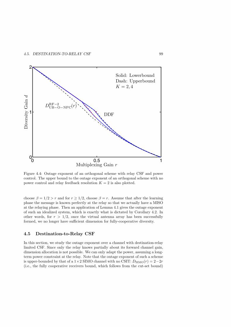
4.5. DESTINATION-TO-RELAY CSF 99
0 0.5 10
1
2
Multiplexing Gain r
Div
ersi
tyG
ain
d
DDF
Solid: LowerboundDash: UpperboundK = 2, 4
DRF−2UB−O−NPC(r)
Figure 4.4: Outage exponent of an orthogonal scheme with relay CSF and powercontrol. The upper bound to the outage exponent of an orthogonal scheme with nopower control and relay feedback resolution K = 2 is also plotted.
choose β = 1/2 > r and for r ≥ 1/2, choose β = r. Assume that after the learningphase the message is known perfectly at the relay so that we actually have a MISOat the relaying phase. Then an application of Lemma 4.1 gives the outage exponentof such an idealized system, which is exactly what is dictated by Corollary 4.2. Inother words, for r > 1/2, once the virtual antenna array has been successfullyformed, we no longer have sufficient dimension for fully-cooperative diversity.
4.5 Destination-to-Relay CSF
In this section, we study the outage exponent over a channel with destination-relaylimited CSF. Since only the relay knows partially about its forward channel gain,dimension allocation is not possible. We can only adapt the power, assuming a long-term power constraint at the relay. Note that the outage exponent of such a schemeis upper-bounded by that of a 1×2 SIMO channel with no CSIT: DSIMO(r) = 2−2r(i.e., the fully cooperative receivers bound, which follows from the cut-set bound)

100CHAPTER 4. D–M TRADEOFF IN DECODE–AND–FORWARD RELAY
CHANNELS
because the source does not know its two forward channel gains.Let β ∈ (max(r, 1/2), 1) be the fraction of dimension allocated for the learning
phase, and K be the resolution of the destination-relay CSF link. At the destina-tion, given g, γ2, an index mapping I(g, γ2) produces an index that is sent back tothe relay. Note that the destination does not know the source-relay channel gain.The relay employs an index-to-power mapping
P : {1, . . . ,K} → {P1, . . . , PK}
where P1 < · · · < PK . We consider the following index mapping.
I(g, γ2) =
⎧⎪⎨⎪⎩
1 if β log(1 + gSNR) + (1− β) log(1 + γ2PK) < r log SNR,min k ∈ {1, . . . ,K}s.t. β log(1 + gSNR) + (1− β) log(1 + γ2Pk) ≥ r log SNR otherwise.
That is, the destination informs the relay to use the smallest power level possible tohelp the transmission, assuming pessimistically that the source-relay link is not inoutage. If the channel is too costly (in a too deep fade) to compensate for, then thesmallest index is sent back to save power. If the source-relay link is in outage thenthe relay, which knows about this event since it has perfect receiver CSI, simplyignores the feedback index I(g, γ2).
The outage exponent of the proposed scheme is given in the following. Theproof is presented in Appendix 4.E.
Proposition 4.6. The optimal outage exponent of the proposed orthogonal schemewith destination-to-relay resolution feedback K is
DDRF-KO-PC (r) = sup min
β∈[max(1/2,r),1)
(2(
1− rβ
),DK
)(4.26)
where
Dk =
⎧⎨⎩2 +Dk−1 − r
1−β if 12 ≤ β < 1− r
1+Dk−11−ββ Dk−1 + 1−r
β if β ≥ max(
12 , 1− r
1+Dk−1
) (4.27)
with the convention D0 = 0.The optimal outage exponent of the proposed nonorthogonal scheme is
DDRF-KNO-PC (r) = sup min
β∈[max(1/2,r),1)
(2− r − r
β,DK
)(4.28)
with Dk defined as in (4.27).
A major difficulty in finding a closed-form expression for the outage exponent inthis case is the dependency on k and β of the point 1− r
1+Dk−1where the function
Dk changes its behavior, in contrast to the fixed value 1− r when only the source

4.5. DESTINATION-TO-RELAY CSF 101
controls its transmit power (cf. Proposition 4.4). Nevertheless, for small values ofK, it is possible to find explicit expressions for the outage exponent. For example,in the case K = 2 we have
DDRF-2O-PC (r) =
{2− 2r(1+2r)
1+r if r <√
17−18 ,
2− 2r(√r2−2r+2−r)1−r otherwise.
As we will see even for K as small as 2, performance very close to perfect CSF canbe achieved. Furthermore, the outage exponent for the full-CSI feedback case canbe found explicitly as follows.
Proposition 4.7. We have
limK→∞
DDRF-KO-PC (r) =
⎧⎨⎩2(
1− 2r2−r)
if r ≤ 25 ,
2(
1− 8r3r+3+
√9r2−14r+9
)otherwise,
(4.29)
and
limK→∞
DDRF-KNO-PC (r) =
{2− r − 2r
2−r if r ≤ 5−√172 ,
2− r − 4r(2−r)3+√
8r2−16r+9 otherwise.(4.30)
We herein present a proof using an indirect approach based on the observationthat K →∞ indeed means the relay knows both h and h2 perfectly. An alternativeproof is presented in Appendix 4.E where we directly apply Proposition 4.6 andthen take the limit K →∞.
Proof. For the sake of brevity, we present only the orthogonal case. Note that K →∞ is equivalent to a direct mapping from channel gains to the power allocated atthe relay P (g, γ2) .= SNRπ(g,γ2). A change of variables gives a = − log g/ log SNR,α2 = − log γ2/ log SNR. Asymptotically the long-term power constraint at the relayreads
supa≥0,α2≥0
(π(a, α2)− a− α2) ≤ 1.
Since outage probability is a nonincreasing function of π∗(a, α2), we conclude thatthe optimal power exponent π∗(a, α2) = 1 + a+ α2.
The outage event is
Pout(r log SNR) = Pr(O1) + Pr(O2)
where O1 is the event that the relay fails to decode the message and the destinationcannot decode the direct transmission.
Pr(O1) = Pr (β log(1 + γ1SNR) < r log SNR, β log(1 + gSNR) < r log SNR).= SNR−2(1− rβ ).
102CHAPTER 4. D–M TRADEOFF IN DECODE–AND–FORWARD RELAY
CHANNELS
The event O2 happens when the relay succeeds to decode but the combined directand relayed signals cannot be decoded by the destination.
Pr(O2) = Pr (β log(1 + γ1SNR) ≥ r log SNR,
β log(1 + gSNR) + (1− β) log(1 + γ2SNRπ∗(g,γ2)) < r log SNR
)= SNR−D∞ .
Then
D∞ = infa,α2≥0
{a+ α2} s.t. β(1− a)+ + (1− β)(1 + a+ α2 − α2)+ < r
= infa≥0{a} s.t. β(1− a)+ + (1− β)(1 + a) < r
(4.31)
Since mina≥0 β(1−a)++(1−β)(1+a) = 2(1−β) (the minimum is attained at a = 1),the optimization problem finding D∞ is infeasible if r < 2(1−β)⇔ β < 2−r
2 . ThusPr(O2) decays exponentially3 in SNR if β < 2−r
2 because the set of “bad” channelsmaking Pr(O2) decay polynomially in SNR is empty. We now compute the outageexponent for the two cases β < 2−r
2 and β ≥ 2−r2 separately and then take the
maximum one to be DDRF−∞O-PC (r).
Case 1: β < 2−r2 . Due to the constraint β ≥ max(r, 1/2), this case never
happens if r > 23 . For r ≤ 2
3 , since Pr(O2) .= SNR−∞ (the notation means expo-nentially decayed in SNR) we have
D1 = supβ∈[r, 2−r2 )
min(
2− 2rβ,∞)
= supβ∈[r, 2−r2 )
2− 2rβ
= 2− 4r2− r .
Case 2: β ≥ 2−r2 . Solving (4.31), we obtain the explicit outage exponent for
Pr(O2)
D∞ = 1− r2β − 1 .
Noting that 2−r2 >
12 , ∀r ∈ (0, 1), we next solve
D2 = supβ∈[max(r, 2−r2 ),1)
min(
2− 2rβ,
1− r2β − 1
).
For r < 25 , we have max
( 12 , r,
2−r2)
= 2−r2 , then 2 − 2 rβ >
1−r2β−1 , ∀β ∈ [ 2−r
2 , 1).
This gives
D2 = 1− r2 2−r
2 − 1= 1.
3Our notion of exponential decay is extended to also include the case of zero probabilityPr(O2) = 0.

4.5. DESTINATION-TO-RELAY CSF 103
0 0.5 10
1
2
Multiplexing Gain r
Div
ersi
tyG
ain
d
DDF
No feedback
Non-orth. dst-relay feedbackDashed: K → ∞Solid: K = 2, 3
Figure 4.5: Outage exponent of a nonorthogonal scheme with destination-relayCSF.
For r ≥ 25 , the maximin is always the intersection of the two component functions
that lies inside[max
( 2−r2 , r), 1), which turns out to be the largest root of f(β) =
4β2 − 3(1 + r)β + 2r. This gives
D2 = 2− 16r3 + 3r +
√9r2 − 14r + 9
.
Finally, combining Case 1 and Case 2 we have
limK→∞
DDRF-KO-PC (r) =
{max(D1,D2) if r < 2
3 ,
D2 otherwise
={
2− 4r2−r if r < 2
5 ,
2− 16r3+3r+
√9r2−14r+9 otherwise.
In Fig. 4.5, the outage exponents of the proposed nonorthogonal schemes areplotted. Indeed the performance in the three cases K = 2, K = 3 and K → ∞ is

104CHAPTER 4. D–M TRADEOFF IN DECODE–AND–FORWARD RELAY
CHANNELS
SS DD
RR
hh
h1h2
I(h; h2) I(h; h2) ´ I(h)
Figure 4.6: The two cooperative upper bounds in the destination-to-source-and-relay CSF scenario. Since the feedback quantizer at destination does not know h1,the feedback index I only depends on h and h2.
practically indistinguishable. This suggests the use of a single bit of feedback (K =2) for power control in the proposed DF scheme to achieve a near optimal diversity-multiplexing tradeoff with very low complexity. A more important and interestingobservation is that the performance is strictly better than DDF for sufficiently larger. While the gain is marginal, it is worth noting that this is realizable even withK = 2. With K = 2, over the range r > 0.65 (rounded up value) the proposednonorthogonal CSF scheme dominates DDF. Thus for low-rate-CSF, high-data-ratesystems, destination-relay feedback is more beneficial than relay-source feedback ina diversity-multiplexing tradeoff sense.
With perfect CSF, however, Proposition 4.7 also shows that the DF with powercontrol at the relay cannot achieve the multiantenna upper bound. In this perfect-CSF scenario, it is better to use compress-and-forward to achieve the optimaldiversity-multiplexing tradeoff of the relay channel [YE07]. It is not yet clear howthe performance of the CF scheme will be affected by the assumption of heavilyquantized CSF considered herein. This remains an interesting topic for future work.
4.6 Destination-to-Source-and-Relay CSF
We now consider the final scenario where the destination broadcasts a feedbackindex to the source and the relay so that both nodes can control their individualpowers. We assume that , the index mapper at the destination depends on thechannel gains h, h2 but not on the source-relay gain h1. Assume a long-term powerconstraint at both the source and the relay.
Before proceeding to the derivation of the achievable outage exponent of anyparticular scheme, it is useful to find an upper bound on the performance of sucha CSF setting. One can naturally think of a fully cooperative MISO channel withfeedback resolution K. Unfortunately, such an upper bound, which is given byDKMISO(r) =
(2 + · · ·+ 2K
)(1− r) = 2
(2K − 1
)(1− r) turns out to be quite loose.
In fact, taking the worst-case of the two cut-set cooperative bounds, we notice that

4.6. DESTINATION-TO-SOURCE-AND-RELAY CSF 105
since the CSF index depends only on g and γ2, the SIMO case where the sourcetransmits and the relay acts as a perfectly cooperating additional receiver is themost restrictive from a diversity exponent viewpoint, as illustrated in Fig. 4.6. Wepresent a tighter upper bound in the following, obtained by considering a SIMOchannel with K feedback levels where a restricted feedback quantizer knows onlyone of the two scalar channel gains.
Lemma 4.2. Assume destination-to-source-and-relay CSF and power control atboth the source and the relay. If the feedback quantizer at the destination does notdepend on the source–relay gain, then the outage exponent with K feedback levels isupper-bounded by
DDSRF-KUB-SPC-RPC(r) = 2K(1− r). (4.32)
Proof. To get an upper bound, we let the relay and the destination fully cooperateand compute the outage exponent DDSF-K
UB-SPC-RPC(r) of the resulting equivalent chan-nel. The equivalent 1× 2 SIMO channel (see Fig. 4.6) has the following properties:
• Squared magnitudes of channel gains λ1 = SNR−a1 and λ2 = SNR−a2 areindependent exponentially distributed random variables with unit variance.
• Perfect CSI at the receiver.• An index mapping I(λ1) produces a feedback index depending on λ1 but
independent of λ2. The feedback link is noiseless, and has zero delay.• A long-term power constraint at the transmitter.Let the K possible transmit power levels be Pk = SNRpk with 1 = p1 < p2 <
· · · < pK < pK+1 = ∞. Let Rk be the kth quantization region, i.e., the set of ofall channel realizations that are mapped to index k. Because the power levels usedat the transmitter depend on λ1 and not on λ2, the long-term power constraint(asymptotically) becomes
sup{a1≥0}∩Rk
(pk − a1) ≤ 1.
Since outage probability is a nonincreasing function of power, the quantizationregion Rk is given by the set of all a1 where SNRpk can be applied but not SNRpk+1 .That is,
Rk = {a1 : pk − 1 ≤ a1 < pk+1 − 1}. (4.33)The constraint a1 ≥ 0 always satisfies since pk ≥ 1, ∀k. Let Pr(outage, I = k) .=SNR−Dk , then the overall outage exponent is given by the slowest decaying termmin(D1, . . . , DK). We then have
Pr(outage, I = k) .= Pr(log(1 + SNRpkλ1 + SNRpkλ2) < r log SNR, I = k).
This leads to
Dk = infa1∈Rk,a2≥0
(a1 + a2) s.t. max((pk − a1)+, (pk − a2)+) < r. (4.34)

106CHAPTER 4. D–M TRADEOFF IN DECODE–AND–FORWARD RELAY
CHANNELS
We distinguish two cases. First, if pk+1−1 < pk−r then (4.34) is infeasible becauseof (4.33). In other words, the set of “bad” channels making Pr(outage, I = k) decaypolynomially in SNR is empty, and by convention Dk =∞. Second, if pk+1 − 1 ≥pk − r then Dk = 2pk − 2r. Since p1 < · · · < pK , the second case does not happenfor any k ∈ {1, . . . ,K − 1}, otherwise the regions Rk+1, . . . ,RK are completelyredundant and increasing K does not increase diversity gain. Therefore we musthave D1 = ∞, . . . , DK−1 = ∞ and DK = 2pK − 2r. Then min(D1, . . . , DK) =2pK−2r is maximized when pK is maximized. This happens when pk+1 = 1+pk−r − εk, k = 1, . . . ,K − 1 where εk > 0 is arbitrarily small. Recalling that p1 = 1,we let εk ↓ 0 and recursively obtain pk = k − (k − 1)r, k = 2, . . . ,K. Finally
DDSF-KUB-SPC(r) = 2pK − 2r = 2K − 2(K − 1)r − 2r = 2K(1− r).
A key observation from Lemma 4.2 is that the diversity gain of a relay channelwith destination-to-source-and-relay CSF increases no faster than linearly in K,which is similar to the behavior of a SISO channel, DKSISO(r) = K(1 − r). On thecontrary, the diversity gain of a MISO or SIMO channel increases exponentiallyin the feedback resolution K, DKSIMO(r) = 2
(2K − 1
)(1 − r). Thus not knowing
the source-relay gain at the destination, which is a relatively realistic assumption,severely affects the diversity performance of the relay channel with CSF.
We now show that the bound DDSRF-KUB-SPC-RPC(r) can be approached by studying
a particular strategy. Going back to the original relay channel, we consider thefollowing index mapping
I(g, γ2) ≡ I(g) ={K if log (1 + gPK−1) < r log SNR,min{k ∈ {1, . . . ,K − 1} : log (1 + gPk) ≥ r log SNR} otherwise.
That is, the source uses the smallest power in {P1, . . . , PK} so that the directtransmission succeeds (using full dimension βk = 1, k = 1, . . . ,K − 1, i.e. norelaying is necessary). If direct transmission would fail even with the largest powerPK , then relaying is used. In this rare event, a fraction of dimension βK = β isassigned to the learning phase.
Optimizing over β leads to the following result.
Proposition 4.8. Assuming both power control at the source and at the relay, theproposed orthogonal scheme with destination-to-source-and-relay feedback resolutionK has an outage exponent of
DDSRF-KO-SPC-RPC(r) =
{2K − (2K + 1)r if r < K
K+2 ,2K(1−r)[K−(K−1)r]
K−(K−2)r otherwise.(4.35)
The nonorthogonal scheme has an outage exponent of
DDSRF-KNO-SPC-RPC(r) =
{2K −
(2K +
√5−12
)r if r < (3−√5)K
(3−√5)K+(√
5−1) ,K(1−r)[2K−(2K−1)r)]
K−(K−1)r otherwise.(4.36)
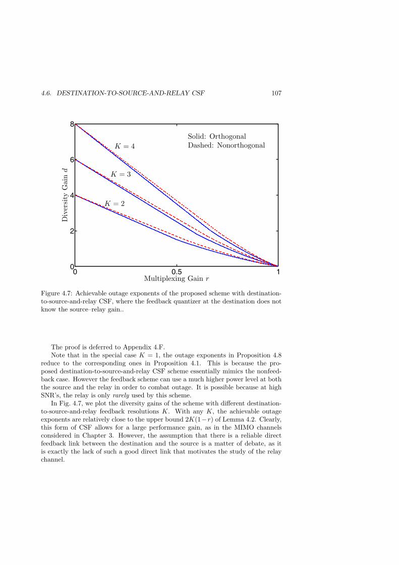
4.6. DESTINATION-TO-SOURCE-AND-RELAY CSF 107
0 0.5 10
2
4
6
8
Multiplexing Gain r
Div
ersi
tyG
ain
d
K = 4
K = 3
K = 2
Solid: OrthogonalDashed: Nonorthogonal
Figure 4.7: Achievable outage exponents of the proposed scheme with destination-to-source-and-relay CSF, where the feedback quantizer at the destination does notknow the source–relay gain..
The proof is deferred to Appendix 4.F.Note that in the special case K = 1, the outage exponents in Proposition 4.8
reduce to the corresponding ones in Proposition 4.1. This is because the pro-posed destination-to-source-and-relay CSF scheme essentially mimics the nonfeed-back case. However the feedback scheme can use a much higher power level at boththe source and the relay in order to combat outage. It is possible because at highSNR’s, the relay is only rarely used by this scheme.
In Fig. 4.7, we plot the diversity gains of the scheme with different destination-to-source-and-relay feedback resolutions K. With any K, the achievable outageexponents are relatively close to the upper bound 2K(1−r) of Lemma 4.2. Clearly,this form of CSF allows for a large performance gain, as in the MIMO channelsconsidered in Chapter 3. However, the assumption that there is a reliable directfeedback link between the destination and the source is a matter of debate, as itis exactly the lack of such a good direct link that motivates the study of the relaychannel.

108CHAPTER 4. D–M TRADEOFF IN DECODE–AND–FORWARD RELAY
CHANNELS
4.7 On Finite-length Codes
A major obstacle in finding codes and schemes with finite length that can achievean error probability that decays in SNR as fast as the outage probability does isthat with a given finite T , the dimension cannot be divided arbitrarily. In factfor a fixed T , we can only allocate the fraction of dimension from a finite, discreteset of rational numbers. In the following, we present some results towards theachievability of the outage exponents in this work with finite-length codes.
For simplicity of presentation, we first consider the orthogonal DF scheme withno CSF. The techniques used in the proof are readily extendable to the CSF cases(see Chapter 3), which we omit as they do not offer any additional insight into theproblem.
Proposition 4.9. With no CSF, there exist orthogonal codes using T ≥ 2 channeluses that achieve the following diversity gain
maxβ∈B
min(
2(
1− rβ
),D2
)
where
D2 =
⎧⎪⎨⎪⎩
2− rβ if β < 12
1−rβ if r > 1− β, β ≥ 1
2 ,
2− r1−β if r < 1− β, β ≥ 1
2
and
B ={T1
T: T1 ∈ {max(Tr, �T/2�),max(Tr, �T/2�) + 1, . . . , T − 1}
}.
Proof. Step 1 - Preliminaries: Let T2 = T − T1 and β = T1T . For convenience
we repeat the communication protocol herein. An encoder is a mapping from amessage to a codeword in codebook C, m → (
√SNRx1,
√SNRxR) where x1 =
[x1(1) · · · x1(T1)] and xR = [xR(1) · · · xR(T2)] are the normalized code-words. Note that C is simply the combination of C1, CR in Section 4.3, normalizedby√
SNR. The individual power constraints read
1|C|T
∑C
T1∑n=1|x1(n)|2 ≤ 1,
1|C|T
∑C
T2∑n=1|xR(n)|2 ≤ 1.
Recall that the destination knows whether the source-relay link is in outage ornot, i.e., if β log(1 + γ1SNR) ≥ r log SNR. If β log(1 + γ1SNR) ≥ r log SNR then

4.7. ON FINITE-LENGTH CODES 109
the entire received signals (a sequence of length T ) are used for decoding at thedestination, otherwise only the received signals in the learning phase (length T1)are used for decoding.
Let us define three events A = {β log(1 + SNRg) < r log SNR}, A1 = {β log(1 +SNRγ1) < r log SNR}, and A2 = {β log(1 + SNRg) + (1 − β) log(1 + SNRγ2) <r log SNR}. The probability of error, over the randomness of the channel gains, thenoise, and the (uniformly distributed) messages can be written as
Pr(ε) = Pr(ε,A1) + Pr(ε, A1)= Pr(ε,A1,A) + Pr(ε,A1, A) + Pr(ε, A1,A2) + Pr(ε, A1, A2)≤ Pr(A1,A) + Pr(ε,A1, A) + Pr(A1,A2) + Pr(ε, A1, A2, εR)
+ Pr(ε, A1, A2, εR)≤ Pr(A1,A) + Pr(ε, A|ΔD) Pr(A1) + Pr(A1,A2)
+ Pr(ε, A2|ΔC, εR) Pr(A1, εR) + Pr(A1, εR)
where ε denotes the error event at the destination m �= m, ΔD denotes the eventthat the destination uses only the directly transmitted sequence to decode, ΔC isthe event that the combined received sequences are used for detection. Note thatε = {ε,ΔD} ∪ {ε,ΔC}. Finally εR is the event that the relay makes an incorrectdecision mR �= m. In the last inequality we use Pr(ε, A|A1) = Pr(ε, A|ΔD) andPr(ε, A2|A1, εR) = Pr(ε, A2|ΔC, εR), which follow the protocol of the scheme.
Inspired by the concept of approximately universal codes [TV06], we will nextfind sufficient conditions on the (sequence of) codes C so that Pr(ε, A|ΔD) .=SNR−∞, Pr(εR, A1) .= SNR−∞, and Pr(ε, A2|ΔC, εR) .= SNR−∞. Recall thatf(SNR) .= SNR−∞ denotes an exponentially decaying function of SNR. If such asequence of codes exists, then
Pr(ε) ≤ Pr(A1,A) + Pr(A1,A2)
and by a similar argument as in the outage analysis we readily obtain the resultsin Proposition 4.9, which essentially formulate the maximization of the dominantSNR exponents of Pr(A1,A) + Pr(A1,A2).
At this point, we notice that a simple “shortcut” argument may conclude theproof. The two-phase orthogonal transmission resembles T parallel scalar Gaussianchannels with one channel use. The first T1 scalar channels have a common channelgain h while the remaining T2 channels have a common channel gain h2. But thereexist approximately universal codes CP of length 1 for parallel scalar Gaussianchannels [TV06], thus by definition Pr(ε, A2|ΔC, εR) .= SNR−∞ for those codes.Furthermore, Pr(εR, A1) .= SNR−∞ also holds for the class of codes CP, which canbe seen by considering the special case h2 = 0 (and Pr(ε, A|ΔD) .= SNR−∞ holdswith CP due to symmetry).
In practical terms, one way of achieving the tradeoff in Proposition 4.9 is to usea code of length 1 that is approximately universal for T parallel SISO channels.

110CHAPTER 4. D–M TRADEOFF IN DECODE–AND–FORWARD RELAY
CHANNELS
In the learning phase, the source sends the first T1 symbols (which now span intime rather than in different parallel channels). In the relaying phase, the relaytransmits the remaining T2 symbols (if the source-relay link is not in outage). Aninteresting feature of this approach is that the relay and destination can employidentical decoders. This is especially useful in scenarios where any single node canalternatively act either as relay or destination.
Note however that the above arguments do not directly extend to the nonorthog-onal case, where the two-phase transmission resembles a mixture of SISO and MISOparallel channels. Furthermore, using existing codes for parallel channels is notnecessarily the only way to achieve the tradeoffs in Proposition 4.9. Thus in thefollowing, we present a more general approach to Proposition 4.9 using standardGaussian arguments.
Step 2 - Universal conditions: Let (Δx1,ΔxR) be a nonzero codeword differencevector and perform a change of variable so that ‖Δx1‖2 = SNR−δ1 and ‖ΔxR‖2 =SNR−δR with the convention δ1 =∞ if Δx1 = 0 and δR =∞ if ΔxR = 0.
We claim that if the following two conditions are satisfied(minC
SNR−β(δ1)+)≥ SNR−r (4.37)
(minC
SNR−β(δ1)+SNR−(1−β)(δR)+
)≥ SNR−r (4.38)
then Pr(ε, A|ΔD) .= SNR−∞, Pr(εR, A1) .= SNR−∞, and Pr(ε, A2|ΔC, εR) .=SNR−∞. Recall that by convention 0 .= SNR−∞, thus we must have T1 ≥ 1, T −T1 ≥ 1 otherwise (4.38) cannot be satisfied.
We now prove the above claim. Consider maximum likelihood decoding at bothrelay and the destination, and the following conditional pairwise error probability
Pr(pairwiserelay|h1) = Pr(x1 → x1|h1) ≤ exp(−SNR
2 |h1|2‖Δx1‖2)
= exp(−SNR
2 SNR−α1SNR−δ1)
= exp(−1
2SNR(1−α1)−δ1).
Averaging over α1 ∈ A1 gives
Pr(pairwiserelay, A1) =∫α1∈A1
Pr(pairwiserelay|α1)f(α1)dα1
where f(α1) is the p.d.f. of α1. The subset of channel realizations in A1 makingPr(pairwiserelay, A1) decay polynomially in SNR is
H1 = {α1 ≥ 0 : (1−α1) ≤ δ1}∩ A1 = {α1 ≥ 0 : (1−α1) ≤ δ1, β(1−α1)+ ≥ r+ ε}.

4.7. ON FINITE-LENGTH CODES 111
But due to condition (4.37), there exists a ¯SNR > 0 so that ∀SNR > ¯SNR we have
SNR−β(δ1)+ ≥ SNR−r−ε2
and thus β(δ1)+ ≤ r + ε2 < β(1 − α1)+. This however cannot be satisfied because
∀α1 ∈ H1, (1−α1) ≤ δ1 leading to (1−α1)+ ≤ (δ1)+. We conclude thatH1 is empty,and thus every pairwise error probability, averaged over A1, decays exponentiallyin SNR. Since the number of codewords SNRrT grow only polynomially in SNR,applying the union bound still leads to an exponentially vanishing average errorprobability, Pr(εR, A1) .= SNR−∞. Due to the statistical symmetry of the channel,(4.37) also guarantees that Pr(ε, A|ΔD) .= SNR−∞.
Similarly, by considering the pairwise error probability at the destination
Pr(pairwisedst|ΔC, εR, γ, γ2) ≤ exp(−SNR
2(|h|2‖Δx1‖2 + |h2|2‖ΔxR‖2
))
= exp(−1
2SNR(1−α)−δ1)
exp(−1
2SNR(1−α2)−δR)
and averaging over the nonoutage region A2 = {α, α2 : (1−β)(1−α)++β(1−α2)+ ≥r + ε}, we find that the subset of bad channel realizations in A2 is
H2 = {α ≥ 0, α2 ≥ 0 : (1−α1) ≤ δ1, (1−α2) ≤ δR, (1−β)(1−α)++β(1−α2)+ ≥ r+ε}.
The condition (4.38) means that ∀SNR > ˜SNR for a certain finite ˜SNR, we haveβ(δ1)+ + (1 − β)(δR)+ ≤ r + ε
2 . This leads to a contradiction of the equa-tions defining H2 and thus the subset H2 making the average error probabilityPr(pairwisedestination, A2|ΔC) decay only polynomially in SNR is empty. This leadsto Pr(ε, A2|ΔC, εR) .= SNR−∞.
This concludes the proof of our claim regarding the sufficient conditions (4.37)and (4.38).
Step 3 - Expurgation: We now draw the normalized codewords (x1,xR) froman i.i.d. zero-mean unit-variance complex Gaussian ensemble. The codebook sizeis |C| = SNR(r−ε)T with an arbitrarily small ε > 0. Then we expurgate all badcodewords that lead to the violation of at least one of the approximately universalconditions [Gal65, ZT03].
In particular, we fix the first codeword x0 and compute all codeword differencesx − x0 = (Δx1,ΔxR) = (SNR−δ1 ,SNR−δR). We expurgate x0 if there existsanother codeword so that (δ1, δR) ∈ B1 ∪ B2 where
B1 ={δ1, δR : SNR−β(δ1)+ ≤ SNR−r
},
B2 = {δ1, δR : SNR−β(δ1)+−(1−β)(δR)+ ≤ SNR−r}.We then repeat the process for x1, . . . ,x|C|−1.

112CHAPTER 4. D–M TRADEOFF IN DECODE–AND–FORWARD RELAY
CHANNELS
Over the ensemble, the codeword difference Δx1, ΔxR are i.i.d. zero-meanvariance-2 complex Gaussian random vectors of length T1 and T2 respectively. Wethen have Pr ((δ1, δR) ∈ B1 ∪ B2) .= SNR−De where
De = inf(δ1≥0,δR≥0)∈{B1∪B2}
T1δ1 + T2δR = inf(δ1≥0,δR≥0)∈{B1∪B2}
T (βδ1 + (1− β)δR)
However for SNR > 1, we have
B1 = {δ1, δR : β(δ1)+ ≥ r},B2 = {δ1, δR : β(δ1)+ + (1− β)(δR)+ ≥ r}.
Clearly B1 ∪ B2 = B2, leading to De = Tr. The probability that we expurgate x0
is then union-bounded by
Pr(x0 expurgated) ≤ SNR(r−ε)TSNR−De = SNR−Tε.
Let the indicator function be 1(·). Then the average (over the ensemble) numberof codewords after expurgation is
E
⎡⎣|C|−1∑i=0
(1− 1(xi expurgated)
)⎤⎦ = |C| −|C|−1∑i=0
E[1(xi expurgated)
]
= |C| −|C|−1∑i=0
Pr(xi expurgated
)≥ |C| − |C|Pr
(x0 expurgated
).= |C|
(1− SNR−Tε
).= |C|
where the inequality is due to the fact that the first codeword x0 is more likely tobe expurgated than any other codeword.
The derivations above show that the expurgation progress does not lead to aloss of multiplexing gain (rate) of at least one code in the ensemble. Because ε canbe made arbitrarily close to zero, we conclude that in codes drawn from Gaussianensemble there exists at least a code of rate r log SNR that satisfies both sufficientconditions, provided that T1 ≥ 1 and T2 = T − T1 ≥ 1.
Since the two-phase transmission resembles Gaussian channels in parallel, wecan readily extend the above expurgation process to the case of an arbitrary num-ber of parallel channels and even multiple receive antennas. We then obtain aninteresting by-product:
Corollary 4.3. For parallel SIMO Gaussian channels, there exists at least a se-quence of approximately universal codes with length 1. The codes can be obtainedby expurgating codes drawn from an i.i.d. Gaussian ensemble.

4.7. ON FINITE-LENGTH CODES 113
0 0.5 10
1
2
Multiplexing Gain r
Div
ersi
tyG
ain
d
T = 3T = 18
T = 2 T = 4
DNFO (r)
Figure 4.8: Achievable diversity-multiplexing tradeoff of the orthogonal schemewith no CSF and different finite codeword lengths T . The dotted curve is theoutage exponent DNF
O (r) of Proposition 4.1.
Note that the fact that approximately universal codes of length 1 exist has beenestablished in [TV06] by a QAM permutation argument.
In Fig. 4.8, we plot the achievable diversity-multiplexing tradeoff curves withdifferent codeword length T . Some useful conclusions can be drawn from the results.First, there exist codes achieving the linear segment 2 − 3r of the optimal outageexponent DNF
O (r), given that T = 3N , ∀N ∈ {1, 2, . . .}. And even with a moderatelength T = 18, very close to outage performance at all r can be achieved. Note thatdue to the discreteness of the set B, increasing the length T does not necessarilylead to a better performance at all multiplexing gains. Finally, since the relay isrequired to decode the messagem completely, we cannot achieve a nonzero diversitygain for any r ≥ T−1
T .It is possible to apply the above expurgation process to the nonorthogonal DF
case. However, it turns out that expurgating “bad” codewords from a Gaussianensemble leads to a loss of rate, i.e. the number of remaining codewords is notlarge enough to carry out the information rate r log SNR of the original codebook.

114CHAPTER 4. D–M TRADEOFF IN DECODE–AND–FORWARD RELAY
CHANNELS
This is due to the fact that the relaying phase resembles a multiple transmit antennasystem, where the expurgation process is known to incur loss of rate. Thus at anymultiplexing gain, the Gaussian coding bound in this case is only asymptoticallytight as T → ∞. We state the result in the following, and present a sketch of theproof in Appendix 4.G.
Proposition 4.10. With no CSF, there exist nonorthogonal codes using T ≥ 3channel uses that achieve the following diversity gain
maxβ∈B
min(
2− r − rβ,D2
)
where
D2 =
⎧⎪⎨⎪⎩
2− 2r if β < 12
1−rβ if r > 1− β, β ≥ 1
22− r
1−β if r < 1− β, β ≥ 12
with r = r1− 1
(1−β)Tand
B ={T1
T: T1 ∈ {max(T r, �T/2�),max(T r, �T/2�), . . . ,
min(T − 2,
⌊T − 1
1− r⌋)}}
.
Unlike in the orthogonal case, an achievable curve with a finite T never “touches”the outage upper bound DNF
NO(r) because of the loss of rate in expurgation. In thiscase, it is potential to get close to the outage upper bound and better than theorthogonal upper bound DNF
O (r)) with relatively large codeword lengths (T ≈ 100).For short codes the achievable bound is loose, and it is likely that using morestructured codes will give a much better performance than relying on the Gaussiancoding arguments herein, as evident in the MIMO case [TV06, EKP+06].
4.8 Conclusion
We provide a comprehensive study of decode-and-forward relay channels with dif-ferent forms of quantized channel state feedback. Our results suggest that with thehelp of severely limited channel state feedback, the performance of a three-nodecooperative communication system can be considerably improved even with rela-tively simple decode-and-forward schemes. The construction of explicit codes thatachieve or approach the performance of the outage bounds presented in this work,especially in the nonorthogonal case, remains a topic for future study.

4.A. PROOF OF PROPOSITION 4.2 115
Appendices for Chapter 4
4.A Proof of Proposition 4.2
For simplicity of presentation, let us consider K = 2. Generalizing to K > 2 isstraightforward. Furthermore, we consider only an orthogonal scheme, as the prooffor a nonorthogonal scheme is completely similar.
The outage probability is
Pout(r log SNR) = Pr(O1) + Pr(O2) + Pr(O2)
where
Pr(O1) = Pr(I = 1, β1 log(1 + gSNR) + (1− β1) log(1 + γ2SNR) < r log SNR).= Pr(β1(1− α1)+ ≥ r, β1(1− a)+ + (1− β1)(1− α2)+ < r).= SNR−D1 .
Invoking Lemma 4.1 yields
D1 =
⎧⎪⎨⎪⎩
2− rβ1
if r < β1 <12 ,
1−rβ1
if r ∈ (1− β1, β1), β1 ≥ 12 ,
2− r1−β1
if r < 1− β1, β1 ≥ 12 .
(4.39)
Also,
Pr(O2) = Pr(I = 2, β2 log(1 + γ1SNR) ≥ r log SNR,β2 log(1 + gSNR) + (1− β2) log(1 + γ2SNR) < r log SNR)
.= Pr(β1(1− α1)+ < r, β2(1− α1)+ ≥ r,β2(1− a)+ + (1− β2)(1− α2)+ < r),
leading to
D2 =
⎧⎪⎨⎪⎩
2− rβ2
+ 1− rβ1
if r < β2 <12 ,
1−rβ2
+ 1− rβ1
if r ∈ (1− β2, β2), β2 ≥ 12 ,
2− r1−β2
+ 1− rβ1
if r < 1− β2, β2 ≥ 12 .
(4.40)
Finally
Pr(O3) = Pr(I = 2, β2 log(1 + γ1SNR) < r log SNR, β2 log(1 + gSNR) < r log SNR).= Pr(β1(1− α1)+ < r, β2(1− α1)+ < r, β2(1− α)+ < r).
This leads toD3(r) = 2
(1− rβ2
). (4.41)

116CHAPTER 4. D–M TRADEOFF IN DECODE–AND–FORWARD RELAY
CHANNELS
0.5 1−r 1
1
2−2r
β
2 − r1−β
1−rβ
2 − r − β
Figure 4.9: Bounding techniques in Proposition 4.2.
We again only need to consider βk > 1/2 (cf. Section 4.3). The outage exponentcorresponding to an optimal dimension allocation is therefore given by
D∗out(r) = supmax(r,1/2)≤β1<β2<1
min(D1,D2,D3).
4.B Proof of Proposition 4.3
The upper bound is obtained by showing that
2− r − β ≥ 1− rβ
for all β ∈ [1 − r, 1). To that end, noticing that 1−rβ is convex. Thus over β ∈
[1− r, 1), 1−rβ is upper-bounded by the linear segment between the two end points
(1− r, 1) and (1, 1− r). This linear segment is given by 2− r − β (cf. Fig. 4.9).As for the lower bound, we begin with the following lemma.

4.B. PROOF OF PROPOSITION 4.3 117
Lemma 4.3. The outage exponent DRF−KO-NPC(r) is lower-bounded by
DRF−KLB-O-NPC(r) = sup
min(1/r,2)>x1>···>xK≥1min {(1− r)x1 + 1− rx0, . . . ,
(1− r)xK + 1− rxK−1, 2(1− rxK)}with the convention rx0 = 1. For r ≥ 1/2, this lower bound is tight.
The outage exponent DRF−KNO-NPC(r) is lower-bounded by
DRF−KLB-NO-NPC(r) = sup
min(1/r,2)>x1>···>xK≥1min {(1− r)x1 + 1− rx0, . . . ,
(1− r)xK + 1− rxK−1, 2− r − rxK)}with the convention rx0 = 1. For r ≥ 1/2 this lower bound is tight.
Proof. Consider the orthogonal case. We lower-bound the piecewise function
f(β) ={
2− r1−βk− if β < 1− r,
1−rβ otherwise,
by extending the function 1−rβ over the entire support [max(r, 0.5), 1), as illustrated
in Fig. 4.9. By construction, the bound is tight when r ≥ 1/2. As for r < 1/2, weneed to show that
f1(β) ≡ 2− r
1− β ≥1− rβ≡ f2(β),∀β ∈ (1/2, 1− r).
To that end, note that both f1(β) and f2(β) pass through the points (1/2, 2− 2r)and (1− r, 1). But f1(β) is concave and f2(β) is convex over [1/2, 1− r), we readilyhave f1(β) ≥ f2(β). Finally a change of variable xk = 1/bk gives the claimedbound.
The bounds to DRF−KNO-NPC(r) are obtained in a similar manner.
We now compute the explicit solution to the optimization problems posed inLemma 4.3. Consider the orthogonal case. The problem can in fact be recast asa linear program. The global optimum of the maximin is given by the intersectionof all K + 1 affine functions, provided that the intersection satisfies the linearconstraints min(1/r, 2) > x1 > · · · > xK ≥ 1. Let us find this balancing point.Introduce a variable Δ so that
(1− r)x1 = Δ(1− r)x2 + 1− rx1 = Δ
· · ·(1− r)xK + 1− rxK−1 = Δ
2(1− rxK) = Δ.

118CHAPTER 4. D–M TRADEOFF IN DECODE–AND–FORWARD RELAY
CHANNELS
From the last equation we have
xK = 2−Δ2r . (4.42)
From the first K equations, we have
x2 = Δ− 11− r + r
1− rx1 = Δ− 11− r + r
(1− r)2 Δ = Δ− 11− r
(1 + r
1− r)
+ r
(1− r)2
x3 = Δ− 11− r
(1 + r
1− r +(r
1− r)2)
+ r2
(1− r)3
· · ·
xK = Δ− 11− r
K−1∑k=0
(r
1− r)k
+ rK−1
(1− r)K .
Combining with (4.42) leads to
Δ =1r + 1
1−r∑K−1k=0
(r
1−r)k− rK−1
(1−r)K
12r + 1
1−r∑K−1k=0
(r
1−r)k
=
⎧⎨⎩
2(1−r)−2(1−r)( r1−r )K
1−2r( r1−r )K
if r �= 1/22K
1+2K if r = 1/2.
It can be verified that with this value of Δ, all the linear constraints are satisfied.Thus DRF−K
LB-O-NPC(r) = Δ.Using a similar technique, we can show that
DRF−KLB-NO-NPC(r) =
2−rr + 1
1−r∑K−1k=0
(r
1−r)k− rK−1
(1−r)K
12r + 1
1−r∑K−1k=0
(r
1−r)k
=
⎧⎨⎩
2(1−r)2−(1−r)( r1−r )K
1−r−r( r1−r )K
if r �= 1/21+2K2+2K if r = 1/2.
4.C Proof of Proposition 4.4
We essentially follow the same line of arguments as in the short-term case. The keydifference is the fact that under a long-term power constraint, a power level in theorder of
SNRPr(I(γ1) = k)

4.C. PROOF OF PROPOSITION 4.4 119
can be applied given that the index I(γ1) = k is received at the source [ECD06].Again we only present the case K = 2 to improve readability. Consider an
orthogonal scheme. Let pk be the SNR exponent of power level Pk, i.e. Pk.= SNRpk ,
with 1 = p1 < p2 < ∞. We have Pout(r log SNR) = Pr(O1) + Pr(O2) + Pr(O3).Herein
Pr(O1) = Pr(I = 1, β1 log(1+gP1)+(1−β1) log(1+γ2SNR) < r log SNR) .= SNR−d1
where
D1 ={
1−rβ1
if r ∈ (1− β1, β1), β1 ≥ 12 ,
2− r1−β1
if r < 1− β1, β1 ≥ 12 .
Notice that P1.= SNR1 and that we do not consider β1 < 1/2 for the same reason
as presented in Section 4.3.We now have
Pr(I = 2) = Pr(β1 log(1 + γ1SNR) < r log SNR, β2 log(1 + γ1P2) ≥ r log SNR).= SNR−
(1− r
β1
)where the exponent equality is due to p2 − r
β2> 1 − r
β1, making the probability
of the event {β2 log(1 + γ1P2) < r log SNR} decays to zero faster than that of{β1 log(1 + γ1SNR) < r log SNR}. Then, we have
P2.= SNR
Pr(I = 2) = SNR2− rβ1 .
Let us next compute the SNR exponent D2 of
Pr(O2) = Pr(I = 2, β2 log(1 + γ1P2) ≥ r log SNR,β2 log(1 + gP2) + (1− β2) log(1 + γ2SNR) < r log SNR)
.= Pr(β1(1− α1)+ < r, β2
(2− rβ1− a)+
+ (1− β2)(1− α2)+ < r
)
Using Lemma 4.1, we obtain
D2 ={
1− rβ1
+ 1−rβ2
if r ∈ (1− β2, β2),3− r
β1− r
1−β2if r < 1− β2.
Finally
Pr(O3) = Pr(β2 log(1 + γ1P2) < r log SNR, β2 log(1 + gP2) < r log SNR).= SNR−2
(p2− r
β2
).= SNR−2
(2− r
β1− rβ2
).

120CHAPTER 4. D–M TRADEOFF IN DECODE–AND–FORWARD RELAY
CHANNELS
4.D Proof of Proposition 4.5
We present only the orthogonal case as the nonorthogonal case follows exactly thesame line of arguments. The proof of lower bounds are similar to that in theshort-term power constraint case and thus omitted.
For the lower bound, we first lower-bound the exponent Dk ≥ k − 1 + 1−rβk−∑k−1
i=1rβi
and change variable xk = (βk)−1 (cf. Appendix 4.B). This leads to
DRF−KO-PC (r) ≥ sup min ((1− r)x1, 1 + (1− r)x2 − rx1, . . . ,
K − 1 + (1− r)xK − rK−1∑k=1
xk, 2(K − r
K∑k=1
xk
))
where the supremum is over min(1/r, 2) ≥ x1 > x2 > · · · > xK > 1. We willbalance the K + 1 terms and verify if the solution satisfies the linear constraints.To that end, let
(1− r)x1 = 1 + (1− r)x2 − rx1 = · · ·
= K − 1 + (1− r)xK − rK−1∑k=1
xk
= 2(K − r
K∑k=1
xk
)
= Δ.
Balancing the first K terms leads to
x1 = 1 + (1− r)x2,
x2 = 1 + (1− r)x3,
· · ·xK = 1 + (1− r)xK−1
and thus
x1 = Δ1− r ,
x2 = 11− r
(Δ
1− r − 1),
x3 = 11− r
(Δ
(1− r)2 − 1− 11− r
),
· · ·
xK = 11− r
(Δ
(1− r)K−1 −K−2∑k=0
1(1− r)k
).
(4.43)

4.D. PROOF OF PROPOSITION 4.5 121
Inserting these values into 2(K − r∑Kk=1 xk
)= Δ and simplifying give
Δ =(1− r) (1− (1− r)K)r(1− 1
2 (1− r)K) .With this Δ, we can readily verify that x1 > · · · > xK > 1. However the constraintmin(1/r, 2) ≥ x1 does not always satisfy. In particular,
x1 = Δ1− r =
(1− (1− r)K)r(1− 1
2 (1− r)K) ≤ min(1/r, 2) = 1r,∀r ≥ 1/2
but when r < 1/2,
x1 = Δ1− r =
(1− (1− r)K)r(1− 1
2 (1− r)K) ≤ min(1/r, 2) = 2 iff (1− r)K+1 ≥ 1− 2r.
That is, over {r : (1 − r)K+1 < 1 − 2r} the intersection is not the solution ofthe maximin. Since DRF−K
LB-O-PC(r) ≤ 2− 2r, it suffices to shows that DRF−KLB-O-PC(r) =
2 − 2r over this range of r. Let K ∈ {2, . . . ,K} so that (1 − r)K ≥ 1 − 2r and(1 − r)K+1 < 1 − 2r. Such a K always exists because (1 − r)2 ≥ 1 − 2r,∀r and(1− r)K+1 < 1− 2r by assumption.
Inserting Δ = 2− 2r into (4.43) we obtain
x1 = 2,
x2 = 11− r ,
· · ·
xK = 11− r
(2
(1− r)K−2 −K−2∑k=0
1(1− r)k
).
Note that 2 ≥ x1 > x2 > · · · > xK . Furthermore, with the given K, we can easilycheck that
xK = 11− r
⎛⎝ 2
(1− r)K−2−K−2∑k=0
1(1− r)k
⎞⎠ ≥ 1
andxK+1 < 1.
We now show that min(D1, . . . , DK , 2
(K − r∑Kk=1 xk
))= 2 − 2r with the
choicex1 = x1, x2 = x2, . . . , xK = xK , xK+1 = · · · = xK = 1.
Note that this choice of {xk} satisfies all the linear constraints.

122CHAPTER 4. D–M TRADEOFF IN DECODE–AND–FORWARD RELAY
CHANNELS
By construction we have D1 = · · · = DK = 2− 2r. Furthermore,
DK+1 −DK = (1− r)xK+1 + 1− xK > (1− r)xK+1 + 1− xK = 0
thus we have DK+1 > DK = 2− 2r. For l > K + 1 we have
Dl −Dl−1 = (1− r) + 1− 1 = 1− r > 0
thus Dl > Dl−1 > 2− 2r.It remains to show that 2
(K − r∑Kk=1 xk
)≥ 2− 2r ⇔ K− r∑Kk=1 xk ≥ 1− r.
But
K − rK∑k=1
xk = K − rK∑k=1
xk + (K − K)(1− r) ≥ K − rK∑k=1
xk.
With the given {xk}, after some straightforward manipulation we have
K − rK∑k=1
xk ≥ 1− r ⇔ (1− 2r) > (1− r)K+1.
But this always holds given our choice of K.We conclude that over {r : (1− r)K+1 < 1− 2r},
sup2≥x1>···>xK>1
min(D1, . . . , DK , 2
(K − r
K∑k=1
xk
))= 2− 2r.
4.E Destination-Relay CSF
Proof of Proposition 4.6For any K, the outage event is dominated by two terms
Pout(r log SNR) .= Pr(O1) + Pr(O2)
where O1 is the event that the relay fails to decode the message and the destinationcannot decode the direct transmission either.
Pr(O1) = Pr (β log(1 + γ1SNR) < r log SNR, β log(1 + gSNR) < r log SNR).= SNR−2(1− rβ ).
The event O2 happens when the relay succeeds to decode but the combined directand relayed signals cannot be decoded by the destination. Due to the construction

4.E. DESTINATION-RELAY CSF 123
of I(g, γ2), this only happens when I = K, i.e. when largest power level PK isapplied at the relay.
Pr(O2) = Pr (I = K,β log(1 + γ1SNR) ≥ r log SNR,log(1 + gSNR) + (1− β) log(1 + γ2PK) < r log SNR) .
To apply Lemma 4.1 to find the SNR exponent of Pr(O2), we first recursivelycompute the exponent of PK .
We have P1.= SNR, and Pr(I = 2) .= SNR−D1 where D1 is given by Lemma 4.1
D1 ={
2− r1−β if 1
2 ≤ β < 1− r1−rβ if β ≥ max(1/2, 1− r).
Then we have P2.= SNR1+D1 . Invoking Lemma 4.1 again gives Pr(I = 3) .=
SNR−D2 where
D2 ={
2 +D1 − r1−β if 1
2 ≤ β < 1− r1+D1
−D1 + 1+D1−rβ if β ≥ max
(12 , 1− r
1+D1
).
Continuing this line of arguments leads to the claimed result.
Alternative Proof of Proposition 4.7We have
Pout(r log SNR) .= SNR−2(1− rβ ) + SNR−D∞
where D∞ = limk→∞DK with DK defined as in (4.27), i.e.
Dk =
⎧⎨⎩2 +Dk−1 − r
1−β if 12 ≤ β < 1− r
1+Dk−11−ββ Dk−1 + 1−r
β if β ≥ max(
12 , 1− r
1+Dk−1
).
Notice that for any given r, β the sequence (indexed by k) 1 − r1+Dk is increasing
because the sequence Dk is increasing. We consider two cases.Case 1: Assume β > 1 − r
1+D∞ , implying that β > 1 − r1+Dk , ∀k. Then by
definition
D1 = 1− rβ,
D2 = 1− rβ
+(
1β− 1)
1− rβ,
D3 = 1− rβ
+(
1β− 1)(
1− rβ
+(
1β− 1)
1− rβ
),
· · ·
DK = 1− rβ
(1 + 1− β
β+ · · ·+
(1− ββ
)K−1).

124CHAPTER 4. D–M TRADEOFF IN DECODE–AND–FORWARD RELAY
CHANNELS
We can exclude the point β = 1/2 because of the following. With β = 1/2 we haveDK = 2K(1− r)→∞ as K →∞. But we require β = 1
2 > 1− r1+D∞ = 1− 0 = 1,
which is a contradiction. Thus we only consider β > 1/2 meaning that 1−ββ < 1.
Then
DK =(1− r)
(1−(
1−ββ
)K)2β − 1
andD∞ = lim
K→∞DK = 1− r
2β − 1 .
To satisfy β > 1− r1+D∞ we must have
β > 1− r
1 + 1−r2β−1
⇔ β > 2− r2 .
The above condition always holds when r > 2/3, given the constraint β ≥ max(1/2, r).From the indirect proof (cf. Section 4.5), we know that
D2 = sup minβ∈[max(r, 2−r2 ),1)
(2(
1− rβ
),
1− r2β − 1
)
={
1 if r < 25 ,
2− 16r3+3r+
√9r2−14r+9 otherwise.
Case 2: β < 1 − r1+D∞ ⇔ β < 2−r
2 , which only happens when r < 23 . There
exists an integer K ∈ [0,∞) so that
1− r
1 +DK> β ≥ 1− r
1 +DK−1
with the convention 1− r1+D−1
= max(r, 1/2). Then DK > 0 and by definition, wehave
DK+1 = 2 +DK −r
1− β ,
DK+2 = 2 +DK+1 −r
1− β = DK + 2(
2− r
1− β),
· · ·
DK+L = DK + L(
2− r
1− β)
Since β < 2−r2 , we have 2− r
1−β > 0 thus
D∞ = limL→∞
DK+L =∞.

4.F. PROOF OF PROPOSITION 4.8 125
This leads to
D1 = supβ∈[max( 1
2 ,r),2−r
2 )min(
2− 2rβ,D∞
)= supβ∈[max( 1
2 ,r)2−r
2 )
(2− 2rβ
)= 2− 4r
2− r .
Combining D1 and D2 leads to the desired result.
4.F Proof of Proposition 4.8
We present only the proof for an orthogonal scheme. Recall that we use the followingindex mapping
I(g, γ2) ≡ I(g) ={K if log (1 + gPK−1) < r log SNR,min{k ∈ {1, . . . ,K − 1} : log (1 + gPk) ≥ r log SNR} otherwise
and that β is the fraction of dimension assigned to the learning phase (only) whenI = K.
We now show that
DDSF-KO-SPC (r) = sup
β∈[
max(
rK−(K−1)r ,
12
),1)min
(2K − 2(K − 1)r − 2r
β,DK
)(4.44)
where
DK =
⎧⎨⎩2K − 2(K − 1)r − r
1−β if max(
rK−(K−1)r ,
12
)≤ β < 1− r
K−(K−1)rK(1−r)β if β ≥ max
(r
K−(K−1)r ,12 , 1− r
K−(K−1)r
).
To that end, let pk be the SNR exponent of the power level used at the source(and also the relay when I = K) given that I = k. We readily see that p1 = 1,p2 = 1+p1−r = 2−r, . . . , pK = 1+pK−1−r = K−(K−1)r. Due to construction,outage can only happen when I = K thus
Pout(r log SNR) .= Pr(O1) + Pr(O2)
where
Pr(O1) = Pr (I = K,β log(1 + γ1PK) ≥ r log SNR,β log(1 + gPK) + (1− β) log(1 + γ2PK) < r log SNR)
.= SNR−DK .
If βpK < r then the event β log(1+γ1PK) < r log SNR happens with probability inthe order of SNR0, meaning that the relay is completely redundant in the proposedscheme. Therefore we constrain β ≥ r
pK= rK−(K−1)r . Note that the event β log(1+

126CHAPTER 4. D–M TRADEOFF IN DECODE–AND–FORWARD RELAY
CHANNELS
gPK) + (1− β) log(1 +PKSNR) < r log SNR implies β log(1 + gPK−1) < r log SNRor I = K. Invoking Lemma 4.1 yields
DK =
⎧⎨⎩2K − 2(K − 1)r − r
1−β if max(
rK−(K−1)r ,
12
)≤ β < 1− r
K−(K−1)rK(1−r)β if β ≥ max
(r
K−(K−1)r ,12 , 1− r
K−(K−1)r
).
Similarly
O2 = {I = K,β log(1 + γ1PK) < r log SNR, β log(1 + gPK) < r log SNR} ,
which givesPr(O2) .= SNR−2(pK− rβ ) = SNR−2(K−(K−1)r− rβ ).
Inserting into (4.44) and solving for the optimal β∗ yield β∗ = 2/3 for r < KK+2
and β∗ = K−(K−2)r2K−2(K−1)r for r ≥ K
K+2 . This leads to the claimed results.
4.G Proof of Proposition 4.10
Since the proof follows closely that of Proposition 4.9, we briefly summarize themain steps herein.
Step 1 - Preliminaries. Let β = T1/T ≥ 1, T2 = (1 − β)T ≥ 2. An encoder isa mapping m→ √SNR(x1,X2) where X2 is a T2 × 2 matrix with the first row x21being the sequence sent from the relay and the second row x22 being the sequencesent from the source during the relaying phase. The power constraints are
1|C|T
∑C
(‖x1‖2 + ‖x22‖2) ≤ 1,
1|C|T
∑C‖x21‖2 ≤ 1.
Step 2 - Universal conditions. Consider a codeword difference (Δx1,ΔX2).Let ‖Δx1‖2 = SNR−δ1 and let λ2 = SNR−δ2 be the smallest squared singular valueof ΔX2. Applying again the Chernoff bound and using the worst-case rotationargument [TV06], we end up with the conditions(
minC
SNR−β(δ1)+)≥ SNR−r, (4.45)
(minC
SNR−β(δ1)+SNR−(1−β)(δ2)+
)≥ SNR−r. (4.46)
Step 3 - Expurgation. Draw (x1,X2) from an i.i.d. zero-mean unit-variancecomplex Gaussian ensemble. The probability that a codeword difference is too

4.G. PROOF OF PROPOSITION 4.10 127
small leading to the expurgation of a codeword, Pr((Δx1,ΔX2) ∈ B), has an SNRexponent of (recall that ΔX2 in this case is a T2 × 2 matrix)
infδ1≥0,δ2≥0
T1δ1 + (T2 − 1)δ2
s.t. T1δ1 + T2δ2 ≥ Tr,
which is optimized at δ∗1 = 0, δ∗2 = TT2r, leading to
Pr((Δx1,ΔX2) ∈ B) .= SNR−T2−1T2Tr.
To make the average number of expurgated codewords insignificant compared tothe number of codewords before expurgation, we require the original codebook sizeto be SNRrT , where
r = T2 − 1T2r − ε =
(1− 1
(1− β)T)r − ε
for an arbitrarily small ε > 0. The expurgated code itself is therefore not ap-proximately universal because its multiplexing gain strictly is less than r (even ifε = 0). However we can conclude that when this expurgated code of rate r log SNRis used, an SNR exponent of the error probability min(2−r−r/β,D2) is achievable,where r < r (strict inequality). In other words, as long as the mutual information isgreater than r log SNR > r log SNR, then the expurgated code has Pr(ε) .= SNR−∞.This leads to the claimed result.
On a final note, the constraint T1 ≤ min(T − 2,
⌊T − 1
1−r⌋)
in the maximin ofProposition 4.10 is due to the fact that we constrain T2 ≥ 2 and that we requirethe multiplexing gain r
1− 1(1−β)T
< 1. Clearly, as in Chapter 3, this expurgationprocedure is only applicable for sufficiently small r.


Chapter 5
D–M Tradeoff inCompress–and–Forward RelayChannels
We continue the D–M tradeoff analysis with another relaying protocol in this chap-ter. It is shown in [YE07] that the compress-and-forward strategy achieves thefull cooperative D–M tradeoff bound of a three-node wireless relay network. Thisis obtained under the possibly unrealistic assumption that the relay has perfectknowledge of all three channel coefficients (source-destination, source-relay andrelay-destination), and that the destination has perfect knowledge of the source-relay channel coefficient. Also, in the optimal CF strategy the relay makes useof Wyner-Ziv source coding with side information. This chapter investigates theachievable D-M tradeoff of the same network, under the same assumptions of perfectchannel state information, when the relay is constrained to make use of standard(non-WZ) source coding. It is shown that under a short-term power constraint atthe relay, using source coding without side information results in a significant lossin terms of the D–M tradeoff. For multiplexing gains r ≤ 2
3 , this loss can be fullycompensated for by relaxing the power constraint to a long-term one, and by usingpower control at the relay. On the contrary, for large multiplexing gain r ∈ ( 2
3 , 1)
the loss with respect to WZ coding remains strict.
5.1 Introduction
In [YE07], it is shown that the multiple-antenna relay network achieves the co-operative upper bound (fully cooperative transmit antennas) by using a compressand forward strategy, where the relay sends to the destination a source-encoded(lossy) version of its received signal, which is then treated by the destination as anadditional observation and used to decode the source information message. Theoptimal CF strategy makes use of Wyner-Ziv source coding with side information
129

130CHAPTER 5. D–M TRADEOFF IN COMPRESS–AND–FORWARD RELAY
CHANNELS
at the relay, and its optimality is shown under the critical assumption that the relayknows both the channel matrix from relay to destination and that from source todestination. It is also necessary that the destination knows the channel matrix fromsource to relay.
The practical implementation of WZ source coding with side information isgenerally much more complex than standard source coding. Since WZ coding re-quires a channel decoding operation at the decoder, approaching the rate-distortionlimit in this case requires large block length and significant encoding and decodingcomplexity (see for example [WO01, MB02, CPR03, YCXZ03, CX05]).
At this point, it is legitimate to ask the following question: “How much of theoptimality of the CF strategy in [YE07] comes from WZ coding, and how muchcomes from CSI at the relay?.”
In this chapter, we quantify the D-M tradeoff loss incurred by not using WZcoding at the relay. We thus indirectly show that source coding with side infor-mation as in [HZ05, YE07] is instrumental in achieving a superior performanceover quasi-static fading relay channels. However, the picture is not as bleak asit may appear. By relaxing the power constraint at the relay from peak (short-term) to average (long-term) and allowing power control, we show that the non-WZ CF strategy achieves the optimal cooperative D–M tradeoff for all multiplex-ing gain r ≤ 2
3 and generally outperforms the best known AF and DF strategies[AES05, LTW04, KCS07b].
Our results indicate that simple CF strategies based on scalar quantization andpower control at the relay, coupled with clever protocols that distribute the requiredchannel state information to the relay and to the destination, can indeed achievevery good practical throughput and reliability performance with low complexity.
5.2 System Model
Consider a three-node slowly fading wireless relay channel. All terminals have asingle antenna, and are constrained to operate in half-duplex mode [LTW04]. Thesource-destination, source-relay, and relay-destination channel gains are denotedby h, h1, and h2 respectively. The channel is statistically symmetric, with h, h1,and h2 being mutually independent complex Gaussian random variables with zeromean and unit variance. The channel is constant during a fading block of T chan-nel uses, and changes independently from one block to the next. Again, we areinterested in the high-SNR performance of this channel when the allowed decodingdelay is equal to T . Since the fading is constant over blocks of T symbols, the er-ror probability performance is dominated by the outage probability. Furthermore,we consider the case of large block length T , for which the information theoreticlimits of channel coding and rate-distortion source coding are achievable by stan-dard random Gaussian coding. Since we look at both large SNR and large T , thelimit ordering becomes important. Conceptually, we may think of an increasingsequence of operating SNRs, and for each SNR we look at the system performance

5.2. SYSTEM MODEL 131
when T → ∞. All three channels are affected by additive white noises, mutuallyindependent and identically distributed, with with complex circularly symmetricGaussian components ∼ CN (0, 1). It is well-known that in the quasi-static largeT regime each receiver can estimate with vanishing loss its own channel coefficient[BPS98]. Therefore, with no loss of generality, we assume perfect CSI at all receivers(relay and destination).
We study a CF scheme under the assumptions made in [YE07], that the relayknows h and h2 perfectly, and that the destination has perfect knowledge of thesource-relay gain h1. First, we consider the case of a peak (or short-term) powerconstraint, where the relay codewords are constrained to satisfy
1T |C|
∑sR∈C‖sR‖2 ≤ SNR
in each fading block. Then, we relax this to an average (or long-term) powerconstraint, given by
1T |C|
∑sR∈C
E[‖sR‖2
] ≤ SNR
where the expectation is with respect to the fading statistics. This relaxed con-straint allows for the use of power control at the relay, where in certain fadingblocks a power much larger than average can be used, provided that the averageconstraint is satisfied.
The information rate of the source is r log SNR bit per channel use, which isfixed for a given SNR. Recall that an outage event occurs when the mutual informa-tion between source and destination is smaller than r log SNR. The correspondingprobability of outage is denoted as Pout(r log SNR). We recall that the systemachieves an outage exponent of d when
Pout(r log SNR) .= SNR−d.
Due to the half-duplex constraint, the transmission is divided into two phase.Phase 1 uses a fraction β ∈ (0, 1) of the available degrees of freedom (i.e., it usesβT channel uses), in which the source encodes an equally likely message m ∈{1, . . . , 2rT log SNR} to a codeword sm and then transmits the first βT symbols ofsm. The received signals at the destination and at the relay are
y1 = hs1 + w1
yR = h1s1 + wR (5.1)
respectively, where we omit the time index for brevity.In Phase 2, the source transmits the remaining (1− β)T symbols s2. The relay
vector-quantizes the signal vector received during Phase 1, denoted as yR, andencodes the resulting quantization index into a codeword sR of length (1 − β)T ,transmitted over the relay-destination channel. Notice that the source–channel

132CHAPTER 5. D–M TRADEOFF IN COMPRESS–AND–FORWARD RELAY
CHANNELS
coding used by the relay is a purely digital “tandem” encoding [MP02] approach.The channel code rate is (smaller than but arbitrarily close to)
R0 = log(
1 + |h2|2SNR1 + |h|2SNR
),
The channel bandwidth to source bandwidth ratio for this tandem source-channelcoding scheme is 1−β
β .The destination in Phase 2 observes the signal
y2 = hs2 + h2sR + w2
The decoder at the destination first decodes the quantization index sent by therelay by decoding sR from y2, treating the source codeword as additive Gaussiannoise. Then, assuming that the relay codeword is correctly decoded, it decodes thesource information message m based on the joint observation (y1,y′2, yR) wherey′2 = y2−h2sR and yR is the reconstructed (quantized) version of the relay receivedsignal during Phase 1.
Since this relaying scheme does not use Wyner–Ziv source coding with sideinformation [WZ76, Wyn78] as in [HZ05, YE07] we refer to it as the non-WZ CFscheme.
The vector quantization codebook at the relay is randomly generated, accordingto the probability distribution of
yR = yR − wQ = yR − (cyR + u)
where c = 2−1−ββ R0 and u is a zero-mean complex Gaussian, independent of yR,
with variance σ2u = (1 + |h1|2SNR) (1− c) c. With this choice, the test (backward)
channel [CT91] is realized and the rate-distortion bound can be achieved. Thequantization error
wQ = yR − yRis then i.i.d. complex Gaussian with zero mean and variance
σ2Q = c2 E[|yR|2] + σ2
u
= 2−1−ββ R0 E[|yR|2]
= (1 + |h1|2SNR)(
1 + |h2|2SNR1 + |h|2SNR
)− 1−ββ
.
Note that wQ is uncorrelated with yR.Rewriting
yR = (1− c)yR − u = (1− c)h1s1 + (1− c)w1 − u,

5.2. SYSTEM MODEL 133
we then determine the achievable mutual information of the strategy as
I(s; y1, y2, yR)
= β log
⎛⎝1 + |h|2SNR + |h1|2SNR
1 + σ2u
(1−c)2
⎞⎠+ (1− β) log(1 + |h|2SNR)
= β log(
1 + |h|2SNR + |h1|2SNR1 + (1+|h1|2SNR)c
1−c
)+ (1− β) log(1 + |h|2SNR)
= β log(
1 + |h|2SNR + |h1|2SNR(1− c)1 + c|h1|2SNR
)+ (1− β) log(1 + |h|2SNR).
(5.2)
Recall that
c = 2−1−ββ R0 =
(1 + |h2|2SNR
1 + |h|2SNR
)− 1−ββ
. (5.3)
Note that in order to achieve this rate, the destination needs to know full CSI,i.e., h, h1, and h2. Computing the outage exponent of the scheme then gives thefollowing result, the detailed proof of which is presented in Appendix 5.3.
Proposition 5.1. Assume the relay knows h2 and h. Then under a short-termpower control at the relay, the non-WZ CF scheme achieves the outage exponent
DCF–∞NPC (r) =
{2− 3+
√5
2 r if r < 3−√52 ,
(1− r)(2− r) otherwise.
It is remarkable that the tradeoff of the CF system coincides exactly with theoutage exponent of a nonorthogonal decode-and-forward relaying scheme with noCSIT. Compared to the D–M tradeoff of the CF scheme using Wyner-Ziv sourcecoding, which is shown to be 2 − 2r in [YE07], this simple CF with no side infor-mation exhibits a large degradation at all multiplexing gains. It is now clear thatWZ coding is the key ingredient in achieving the superior performance of the CFschemes in [HZ05, YE07].
Where does this superior gain come from? Recall from [HZ05] that the achiev-able mutual information of CF using WZ coding is
β
(1 + |h|2SNR + |h1|2SNR
1 + σ2WZ
)+ (1− β) log(1 + |h|2SNR) (5.4)
where the compression noise
σ2WZ = (1 + |h1|2SNR + |h|2SNR)c
(1 + |h|2SNR)(1− c)
=
(1 + |h1|2SNR
1+|h|2SNR
)c
1− c

134CHAPTER 5. D–M TRADEOFF IN COMPRESS–AND–FORWARD RELAY
CHANNELS
with c given by (5.3). Comparing the two achievable rates (5.2) and (5.4), we seethat the only subtle difference lies in their compression noise variances (given thesame value of β). Recall that the compression noise without WZ coding in (5.2) is
σ2NWZ = (1 + |h1|2SNR)c
1− c .
In terms of the SNR exponent, most of the time, i.e. when |h1|2 .= SNR0 and|h|2 .= SNR0, the ratio between the quantization noise variances is σ
2NWZσ2
WZ
.= SNR1.This relatively large difference in turn influences the optimization of β, leading tothe performance loss of the non-WZ CF scheme.
We now relax the short-term power constraint at the relay, allowing the relayto control its transmit power over time based on (perfect) CSIT. In this case, thechannel coding rate from relay to destination becomes
RPC0 = log
(1 + |h2|2SNRπ
∗(h,h2)
1 + |h|2SNR
)
where SNRπ∗(h,h2) is the optimal power allocated to the tuple of channel states
(h, h2) fed back from the destination to the relay. Thus the achievable rate issimilar to the no power control case, with a new parameter cPC = 2−
1−ββ R
PC0 . That
is, in this case the noise variance due to quantization decays to zero faster as SNRgrows. We characterize the achievable diversity-multiplexing tradeoff of this schemeby the following result, proved in Appendix 5.4.
Proposition 5.2. Assume the relay knows h2 and h. Then under a long-termpower control at the relay, the non-WZ CF scheme achieves the outage exponent
DCF–∞PC (r) =
{2− 2r if r < 2
3 ,(1−r)(2−r)
r otherwise.
With power control, the simple non-WZ CF approach is optimal for all multi-plexing gains r ≤ 2
3 . What is the intuition behind this phenomenon? The analysisin Appendix 5.4 reveals that for β larger than an r-dependent threshold, the quan-tization noise becomes too large, rendering useless the quantized signal sent fromthe relay. In such cases, no cooperative gain can be achieved (cf. (5.2)). For r > 2
3 ,this threshold on β is strictly less than 1
2 , implying that the relay can contributeswith its own (quantized) received signal observation for less than 1/2 of the avail-able degrees of freedom (as evident from (5.2)), and fully cooperative diversity gaincannot be achieved. The proof in Appendix 5.4 also shows that the probabilityof outage is dominated by the event that the source–destination link alone is in adeep fade. Thus in the high-multiplexing gain regime the bottleneck of non-WZCF relaying with power control is the source–destination link (unfortunately, in
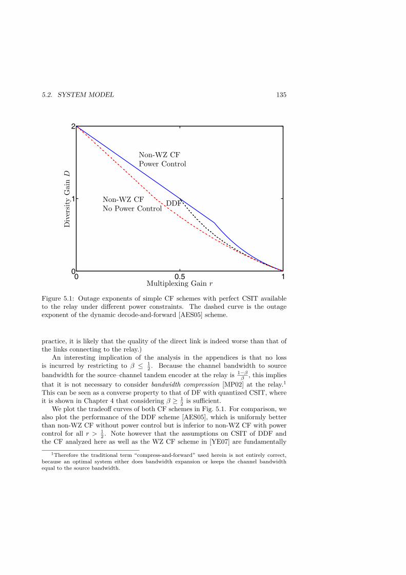
5.2. SYSTEM MODEL 135
0 0.5 10
1
2
Multiplexing Gain r
Div
ersi
tyG
ain
D
Non-WZ CFPower Control
Non-WZ CFNo Power Control
DDF
Figure 5.1: Outage exponents of simple CF schemes with perfect CSIT availableto the relay under different power constraints. The dashed curve is the outageexponent of the dynamic decode-and-forward [AES05] scheme.
practice, it is likely that the quality of the direct link is indeed worse than that ofthe links connecting to the relay.)
An interesting implication of the analysis in the appendices is that no lossis incurred by restricting to β ≤ 1
2 . Because the channel bandwidth to sourcebandwidth for the source–channel tandem encoder at the relay is 1−β
β , this impliesthat it is not necessary to consider bandwidth compression [MP02] at the relay.1This can be seen as a converse property to that of DF with quantized CSIT, whereit is shown in Chapter 4 that considering β ≥ 1
2 is sufficient.We plot the tradeoff curves of both CF schemes in Fig. 5.1. For comparison, we
also plot the performance of the DDF scheme [AES05], which is uniformly betterthan non-WZ CF without power control but is inferior to non-WZ CF with powercontrol for all r > 1
2 . Note however that the assumptions on CSIT of DDF andthe CF analyzed here as well as the WZ CF scheme in [YE07] are fundamentally
1Therefore the traditional term “compress-and-forward” used herein is not entirely correct,because an optimal system either does bandwidth expansion or keeps the channel bandwidthequal to the source bandwidth.

136CHAPTER 5. D–M TRADEOFF IN COMPRESS–AND–FORWARD RELAY
CHANNELS
different.As in [YE07], this work assumes perfect CSIT at the relay, which is a too
optimistic assumption in most practical scenarios. Evaluating the performance ofmore realistic CF relaying schemes with limited feedback remains an interestingtopic for further study.
Appendices for Chapter 5
5.3 Proof of Proposition 5.1
We first state the following convenient lemma without proof.
Lemma 5.1. For β ∈ (0, 1), the linear programming problem
D∗ = infα,α1≥0
{α+ α1} s.t. β(1− α, 1− α1)+ + (1− β)(1− α)+ < r
where (x1, . . . , xn)+ Δ= max(x1, . . . , xn, 0), has solution
D∗ =
⎧⎪⎨⎪⎩
2− 2r if β ≥ 12 ,
1−r1−β if β < min
( 12 , r),
2− rβ if r ≤ β < 12 .
with the corresponding optimizers
(α∗, α∗1) =
⎧⎪⎨⎪⎩
(1− r, 1− r) if β ≥ 12 ,
( 1−r1−β , 0) if β < min
( 12 , r),
(1, 1− rβ ) if r ≤ β < 12 .
We now prove Proposition 5.1. Perform the standard change of variable a =− log |h|2/ log SNR, α1 = − log |h1|2/ log SNR, α2 = − log |h2|2/ log SNR (cf. [ZT03,AES05]). Since
Pout = Pr(β log
(1 + |h|2SNR
+ |h1|2SNR(1− c)1 + c|h1|2SNR
)+ (1− β) log(1 + |h|2SNR) < r log SNR
),
to compute the outage exponent as SNR→∞ we can focus on the set [ZT03]
O ={a, α1, α2 ∈ R
3+ :
β
(1− a, 1− α1 −
(1− α1 − 1− β
β
(1− α2 − (1− a)+
)+)+)+
+(1− β)(1− a)+ < r}.

5.3. PROOF OF PROPOSITION 5.1 137
Herein
c =(
1 + |h2|2SNR1 + |h|2SNR
)− 1−ββ .= SNR−
1−ββ (1−α2−(1−a)+)+
.
The outage exponent is then given by
DCF–∞NPC (r) = min
a,α1,α2∈O(a+ α1 + α2). (5.5)
We partition O into two disjoint regions and solve (5.5) over each region, andthen take the minimum of the two solutions.
Case 1: a ≥ 1. The equation defining O reduces to
β
(1− α1 −
(1− α1 − 1− β
β(1− α2)+
)+)+
< r.
Let D1 be the minimum of the objective function in (5.5) over this region. Wefurther divide Case 1 into two cases.
Case 1.1: 1−α1 <1−ββ (1−α2)+. The optimizers of (5.5) over this subset are
readily found to be (a∗, α∗1, α∗2) =(
1,(
1− rβ , 1− 1−ββ
)+, 0), where we can extend
α∗1 =
⎧⎪⎨⎪⎩
0 if 0 < β < min(r, 1/2),1− 1−β
β if max(1/2, 1− r) < β < 1,1− rβ otherwise.
.
Case 1.2: 1− α1 ≥ 1−ββ (1− α2)+. Similarly we have
(a∗, α∗1, α∗2) =(
1, 0,(
1− rβ, 1− 1− β
β
)+)
and
α∗2 =
⎧⎪⎨⎪⎩
0 if max(1− r, 1/2) < β < 1,1− β
1−β if 0 < β < min(r, 1/2),1− r
1−β otherwise..
Combining Case 1.1 and Case 1.2 leads to
D1 ={
1 + min(
1− rβ , 1− r1−β)
if r < β < 1− r,1 otherwise.
Notice that D1 = 1, ∀r ≥ 12 .
Case 2: a < 1. We now consider
βmax(
1− a, 1− α1 −(
1− α1 − 1− ββ
(a− α2)+)+)
+(1−β)(1−a) < r. (5.6)

138CHAPTER 5. D–M TRADEOFF IN COMPRESS–AND–FORWARD RELAY
CHANNELS
This case is divided into two sub-cases.Case 2.1: 1− α1 <
1−ββ (a− α2)+. Then (5.6) becomes
βmax(1− a, 1− α1) + (1− β)(1− a) < r (5.7)
which does not depend on α2. We easily see that the optimizer α∗2 = 0 and thecondition defining Case 2.1 reduces to 1−α1 <
1−ββ a. The solution to (5.5) under
only the constraint (5.7) is then given by Lemma 5.1 (note that the condition ofCase 2, a < 1, is always satisfied by the solution in Lemma 5.1). It turns out thatthe optimizers in Lemma 5.1 satisfy 1− α∗1 < 1−β
β a∗ iff r + β ≤ 1.
In case r + β > 1, a simple modified version of Lemma 5.1 leads to
(a∗, α∗1) =
⎧⎨⎩(
1− r, 1− 1−ββ (1− r)
)if β ≥ 1/2,(
β1−β , 0
)if β < min(r, 1/2).
In summary, in Case 2.1, the minimum of the objective function in (5.5) is
D(1)2 =
⎧⎪⎪⎪⎪⎪⎪⎨⎪⎪⎪⎪⎪⎪⎩
2− 2r if 12 ≤ β ≤ 1− r,
1−r1−β if β < min(1/2, r, 1− r),2− rβ if r < β < 1/2,1 + 2β−1
β (1− r) if β ≥ max(1/2, 1− r),β
1−β 1− r < β < min(r, 1/2).
Case 2.2: 1− α1 ≥ 1−ββ (a− α2)+. In this case, (5.6) becomes
βmax(
1− a, 1− ββ
(a− α2)+)
+ (1− β)(1− a) < r. (5.8)
Again we note that α∗1 = 0. Now consider the sub-case 1−ββ (a−α2) > 1−a⇔ 1
βa−1−ββ α2 > 1, when (5.8) reduces to (1−β)(1−α2) < r. This leads to the optimizers
of (5.5) (a∗, α∗2) =(
1− r,(
1− r1−β)+)
. In the sub-case 1βa − 1−β
β α2 ≤ 1, (5.8)
becomes (1− a) < r and we also obtain (a∗, α∗2) =(
1− r,(
1− r1−β)+)
. Thus we
have
D(2)2 = 1− r +
(1− r
1− β)+
.
Then D2 = min(D
(1)2 ,D
(2)2
). After some tedious but straightforward manipu-
lation, we have
D2 =
⎧⎪⎪⎪⎪⎨⎪⎪⎪⎪⎩
1−r1−β if β < min
(r, 1−r
2−r),
2− rβ if r < β < 3−√52 ,
1− r if β ≥ 1− r,2− r − r
1−β otherwise.
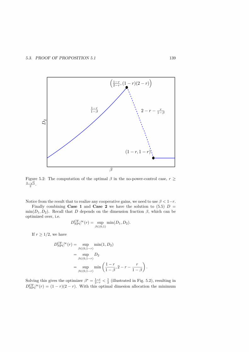
5.3. PROOF OF PROPOSITION 5.1 139
D2
β
1−r1−β 2 − r − r
1−β
(1−r2−r , (1 − r)(2 − r)
)
(1 − r, 1 − r)
Figure 5.2: The computation of the optimal β in the no-power-control case, r ≥3−√5
2 .
Notice from the result that to realize any cooperative gains, we need to use β < 1−r.Finally combining Case 1 and Case 2 we have the solution to (5.5) D =
min(D1,D2). Recall that D depends on the dimension fraction β, which can beoptimized over, i.e.
DCF–∞NPC (r) = sup
β∈(0,1)min(D1,D2).
If r ≥ 1/2, we have
DCF–∞NPC (r) = sup
β∈(0,1−r)min(1,D2)
= supβ∈(0,1−r)
D2
= supβ∈(0,1−r)
min(
1− r1− β , 2− r −
r
1− β).
Solving this gives the optimizer β∗ = 1−r2−r <
12 (illustrated in Fig. 5.2), resulting in
DCF–∞NPC (r) = (1 − r)(2 − r). With this optimal dimesion allocation the minimum

140CHAPTER 5. D–M TRADEOFF IN COMPRESS–AND–FORWARD RELAY
CHANNELS
β
(1 − r, 1 − r)
(1 − r, 1)(r, 1)
D1
D2
(3−
√5
2 , 2 − 3+√
52 r
)
Figure 5.3: The computation of the optimal β in the no-power-control case, r <3−√5
2 .
of (5.5) is attained at either (a∗, α∗1, α∗2) =(
1−r1−β∗ , 0, 0
)= ((1− r)(2− r), 0, 0) or
(a∗, α∗1, α∗2) =(
1− r, 0, 1− r1−β∗
)= (1− r, 0, 1− r(2− r)).
If r ∈[
3−√52 ,
12
), we haveD2 ≤ (1−r)(2−r) < 1 ≤ D1 thus supβ min(D1,D2) =
supβ D2, which also results in DCF–∞NPC (r) = (1− r)(2− r).
If r < 3−√52 , it again turns out that supβ min(D1,D2) = supβ D2, as illus-
trated in Fig. 5.3. This results in β∗ = 3−√52 and DCF–∞
NPC (r) = 2 − 3+√
52 r. The
minimum in (5.5) is attained at (a∗, α∗1, α∗2) =(
1, 1− rβ∗ , 0)
or (a∗, α∗1, α∗2) =(1− r, 0, 1− r
1−β∗)
.
5.4 Proof of Proposition 5.2
The proof is quite similar to the no power control case; and the key steps aresummarized as follows. The power constraint at the relay asymptotically reads
sup {π(a, α2)− a− α2} ≤ 1

5.4. PROOF OF PROPOSITION 5.2 141
which leads to the optimal SNR exponent of the relay transmit power
π∗(a, α2) = 1 + a+ α2.
Recall
cPC =(
1 + |h2|2SNRπ∗(a,α2)
1 + |h|2SNR
)− 1−ββ
.= SNR−1−ββ (π∗(a,α2)−α2−(1−a)+)+
.
We now have DCF–∞PC (r) = infa,α1,α2∈O {a+ α1 + α2} where
O ={a, α1, α2 ∈ R
3+ :
β
(1− a, 1− α1 −
(1− α1 − 1− β
β
(1 + a− (1− a)+)+)+
)+
+(1− β) (1− a)+< r}.
Case 1: a ≥ 1. Then we need to consider the subset defined by
β
(1− α1 −
(1− α1 − 1− β
β(1 + a)
)+)+
< r. (5.9)
Case 1.1: 1 − α1 − 1−ββ (1 + a) < 0 or 2β − 1 < (1 − β)a + βα1. Then
α∗1 =(
1− rβ)+
, α∗2 = 0, a∗ = max(
1, 2β−1−(1− rβ )+
1−β
), and
D(1)1 = max
(1,
2β − 1− (1− rβ )+
1− β
)+(
1− rβ
)+
=
⎧⎪⎪⎪⎪⎨⎪⎪⎪⎪⎩
2− rβ if r < min(β, 3β−4β2
1−β),
1 if β < min(r, 2−r
2),
2β−11−β if (3β−4β2)+
1−β < r < β,r+β−1
1−β if 2−r2 < β < r.
Case 1.2: 2β − 1 ≥ (1− β)a+ βα1 then from (5.9), 1 + a < r1−β . Since a ≥ 1,
this happens only if β ≥ max( 2−r
2 ,23), resulting in D(2)
1 = 1. If β < max( 2−r
2 ,23)
then the problem is infeasible, and we write D(2)1 =∞.
Thus
D1 = min(D
(1)1 ,D
(2)1
)=
⎧⎪⎪⎪⎪⎨⎪⎪⎪⎪⎩
2− rβ if r ≤ β ≤ 23 or β > 2/3, r < 3β−4β2
1−β ,2β−1β if β > 2
3 ,(3β−4β2)+
1−β < r < 2− 2β,r+β−1
1−β if 2−r2 < β <
23 ,
1 otherwise.

142CHAPTER 5. D–M TRADEOFF IN COMPRESS–AND–FORWARD RELAY
CHANNELS
Case 2: 0 ≤ a < 1. We need to consider the constraint
β
(1− a, 1− α1 −
(1− α1 − 1− β
β2a)+)+
+ (1− β) (1− a) < r. (5.10)
Case 2.1: 1 − α1 − 1−ββ 2a ≥ 0 or β ≥ 2(1 − β)a + βα1 then (5.10) becomes
max(β(1− a), (1− β)2a) + (1− β)(1− a) < r. In this case
D(1)2 =
{1− r if β ≥ 2−2r
2−r ,∞ otherwise.
We constrain β < 2−2r2−r from now on, in order to realize any cooperative diversity
gains.Case 2.2: β < 2(1− β)a+ βα1. Then (5.10) reduces to βmax(1− a, 1−α1) +
(1−β)(1− a) < r. Applying Lemma 5.1 yields (recall that we constrain β < 2−2r2−r )
D(2)2 =
⎧⎪⎪⎨⎪⎪⎩
2− 2r if 1/2 ≤ β < 2−2r2−r ,
1−r1−β if β < min
(r, 1
2 ,2−2r2−r),
2− rβ r < β ≤ min(
12 ,
2−2r2−r).
.
Within the range of β < 2−2r2−r , D2 = min
(D
(1)2 ,D
(2)2
)= D(2)
2 .Finally we optimize the dominant exponent of the outage probability:
DCF–∞PC (r) = sup
β∈(0, 2−2r2−r )
min (D1,D2) .
For r < 23 , we readily have DCF–∞
PC (r) = 2 − 2r with the optimizers β∗ = 12 . The
minimum of a+α1 +α2 is attained at (1−r, 1−r, 0) and at (1, 1− 2r) when r < 12 .
When r ∈ [ 12 ,
23), the minimum is attained at (1− r, 1− r, 0) and at (2− 2r, 0, 0).
For r ≥ 23 , some manipulation leads to
DCF–∞PC (r) = sup
β∈(0, 2−2r2−r )
1− r1− β ,
which has the optimizer β∗ = 2−2r2−r ≤ 1
2 . With this β∗, the optimal (a∗, α∗1, α∗2) =((1−r)(2−r)
r , 0, 0)
.

Part III
End-to-end Distortion Exponent
143

Chapter 6
Distortion Exponent over MIMOChannels
In this chapter, the problem of source-channel coding over a multiple-antenna chan-nel with quantized CSIT is considered. As in Chapters 3-5, we focus on the asymp-totically high SNR regime. Upper bounds on the SNR exponent of the end-to-enddistortion achieved with partial CSIT under a long-term power constraint are devel-oped. It is shown that the distortion exponent with perfect CSIT grows unboundedas the ratio between the channel and source bandwidth increases, while the expo-nent achieved with any feedback link of fixed, finite resolution is bounded above bya polynomial of the product between the number of transmit and number of receiveantennas. The resolution of the feedback link should grow with the bandwidthratio to make the distortion exponent scale as fast as that in the perfect-CSITcase. We show that in order to achieve the optimal scaling the CSIT feedback res-olution must grow logarithmically with the bandwidth ratio for MIMO channels,and faster than linear for the single-input single-output channel. The achievabledistortion exponent of some hybrid schemes with heavily quantized feedback is alsoderived. The results demonstrate that dramatic performance improvement over thecase of no CSIT can be achieved by combining simple schemes with a very coarseCSIT feedback.
6.1 Introduction
Consider the problem of source-channel coding over a multiple-antenna fading chan-nel. We focus on the high SNR regime, and adopt the distortion exponent [LMWA05]as the performance measure. Studying the distortion exponent is useful in under-standing the relation between the average end-to-end distortion and the spectralefficiency of the system at high SNR. The analysis is generally carried out under theelegant large-deviation framework of [ZT03], which is originally used to characterizethe diversity-multiplexing tradeoff over multiantenna channels.
145

146 CHAPTER 6. DISTORTION EXPONENT OVER MIMO CHANNELS
The distortion exponent problem has attracted a great deal of interest recently.A simple hybrid digital-analog scheme is proposed and shown to be optimal forhigh-compression systems in [CN05, CN07]. Such HDA joint source-channel codingschemes are first proposed for the broadcast scenario in [MP02]. The advantagespredicted by the theoretical results in [MP02] are later realized by some practicalschemes in e.g., [SPA02, SPA06]. Extensive studies of different layered source-channel coding schemes can be found in [GE05, GE08, BNC06]. Interestingly,layering with superposition coding is shown to be asymptotically optimal in thelimit of infinite superimposed digital layers over a wide range of the ratio betweenthe channel and source bandwidth [GE05, GE08, BNC06]. In practice, however,the complexity and other phenomena inherent to successive decoding such as errorpropagation will likely limit the potentials of such a superposition approach. Theoptimal source-channel rate allocation is also considered in [HG05].
Most previous work assumed only CSIR. While perfect channel knowledge atthe transmitter is generally difficult to obtain, partial CSIT e.g., in the form of a fewfeedback bits, is often available. This motivates the present work where we considera MIMO channel with quantized CSIT, under either a short- or a long-term powerconstraint.
A remarkable feature of the distortion SNR exponent setting is that the presenceof CSIT yields an improvement even in the case of short-term power constraint.This is generally not the case for outage. This is because the outage problem,by its original formulation [OSW94], does not allow rate adaptation1, while thedistortion problem allows instantaneous adaptation of the rate and still results insome improved distortion exponent compared to a no-CSIT system.
In this chapter, we develop upper bounds on the achievable distortion overchannels with partial CSIT. Interestingly, it turns out that with perfect CSIT,under a long-term power constraint, the distortion exponent grows linearly as afunction of the bandwidth ratio. This is in contrast with the short-term powerconstraint case, where the distortion exponent is “saturated” if the bandwidth ratiois sufficiently large. However, our results also show that with any feedback link offixed, finite number of quantization regions (referred to as the feedback “resolution”hereafter), the distortion exponent is bounded above by a polynomial of the productbetween the number of transmit and number receive antennas. It is necessary to letthe feedback resolution grow with the bandwidth ratio to overcome this issue. Wedetermine the rate at which the feedback resolution must grow with the bandwidthratio in order to achieve the same distortion exponent scaling of the perfect CSITbound. In particular, for MIMO systems we show that the resolution must growlogarithmically with the bandwidth ratio, i.e., the number of feedback bits growsonly doubly-logarithmically.
We also study the performance of certain suboptimal hybrid digital-analogsource-channel coding schemes when combined with heavily quantized CSIT. It
1Rate adaptation under the constraint of a minimum rate or a minimum multiplexing gainstill results in a modified outage problem, as presented in Chapter 3.

6.1. INTRODUCTION 147
turns out that over a wide range of practical bandwidth ratios, achieving a signif-icant portion of the perfect-CSIT scheme is possible by combining simple schemeswith a few bits of feedback information. While these schemes are generally sub-optimal, we emphasize that very high distortion exponents are achievable withsignificantly lower complexity than many other no-CSIT techniques. Our resultsalso highlight that even heavily quantized CSIT yields excellent performance whentemporal power control is available.
At this point it is useful to provide a brief summary of our results, classified interms of the bandwidth ratio b (see definition in Section 6.2). In a system with Nttransmit, Nr receive antennas, and feedback resolution K, let m = max(Nt, Nr),n = min(Nt, Nr). Then:
1. For 0 < b ≤ m−n+1n : Proposition 6.1 shows that with perfect CSIT the
distortion exponents with and without power control coincide dPC−∞(b) =dNPC−∞(b). Thus in terms of distortion exponent, even the combinationof perfect CSIT and power control does not help in this very high spectralefficiency regime. Furthermore, this distortion exponent is achievable evenwithout CSIT by a simple HDA scheme in the range b < 1
n [CN05], and bylayering and superposition coding in the range b < m−n+1
n [BNC06]. Thusthe distortion exponent in this regime is completely characterized and wehave the noteworthy result that that CSIT feedback does not increase thedistortion exponent in this range of b.
2. For m−n+1n ≤ b < m− n+ 1: We show that the two exponents with perfect
CSIT still coincide, i.e., dPC−∞(b) = dNPC−∞(b), meaning that in termsof distortion exponent, only rate control is necessary in this regime if fullCSIT is available. Achievable exponents of simple HDA schemes with quan-tized (finite resolution) feedback are derived in Propositions 6.4–6.6. Theseschemes generally do not achieve the upper bounds.
3. For m−n+ 1 ≤ b < mn: We have dPC−∞(b) > dUB−PC−K(b) > dNPC−∞(b)where dUB−PC−K(b) is an upper bound on the distortion exponent of anypower-controlled system with feedback resolution K. This implies that nofixed-resolution feedback schemes can achieve dPC−∞(b). The HDA schemesconsidered in this work generally fall short of achieving dUB−PC−K(b), butyield large improvement compared to no-CSIT schemes, even for coarselyquantized feedback.
4. For b ≥ mn: We have dPC−∞(b) > dUB−PC−K(b) > dNPC−∞(b). It is knownthat layering and superposition coding achieves dNPC−∞(b), even withoutCSIT [GE08]. The achievable distortion exponents under a short-term powerconstraint in Propositions 6.4–6.6 are therefore somewhat redundant. Theachievability of the scheme in [GE08] however comes at the price of highcomplexity in the form of infinitely many superimposed digital layers. Onthe other hand, we show that the use of quantized CSIT feedback allows forlow-complexity schemes that can achieve exponents close to dNPC−∞(b). Theachievable exponents in Propositions 6.4–6.6 under a long-term power con-

148 CHAPTER 6. DISTORTION EXPONENT OVER MIMO CHANNELS
straint are novel. They improve upon dNPC−∞(b) and are close to dPC−∞(b)over a wide range of b, even with very coarse feedback resolution.
6.2 System Model
Consider the transmission of an i.i.d. complex Gaussian source with zero mean andunit variance over a wireless flat-fading channel. The communication system usesNt transmit and Nr receive antennas.
A complex source vector sl of size Ns is generated every T channel uses. Herein,b = T/Ns is the channel bandwidth to source bandwidth ratio, and l is the blockindex. The source vector is mapped to a joint source-channel codeword Xl of sizeNt × T . We consider the case where source blocks are mapped onto codewordsspanning a single fading block, and coding across the fading blocks is forbidden(e.g., because of some strict decoding delay requirement). However, the transmitpower may or may not be averaged over a long sequence of fading blocks (see later).
The complex-baseband received signal during fading block l can be written as
Yl = HlXl + Nl. (6.1)
The components of the Nr × Nt channel matrix Hl are i.i.d. complex Gaussianwith zero mean and unit variance. The channel matrix is constant during a blockof T channel uses, but changes independently from one block to another. Thecomponents of the temporally and spatially white Gaussian noise matrix Nl havezero mean and unit variance. For brevity, we omit the block fading index l wheneverthere is no ambiguity.
Assume perfect knowledge of H at the receiver. Given H, the receiver employsa deterministic index mapping I(H) ∈ {1, . . . ,K} from channel matrix to feedbackindex, where the number of quantization regions K defines the feedback resolution.The feedback index is sent back to the transmitter via a noiseless, zero-delay dedi-cated feedback link, so that at the beginning of each fading block the correspondingindex I(H) is known by the transmitter.
At the transmitter, the power allocation function
P : {1, . . . ,K} → {P1, . . . , PK} (6.2)
maps the feedback index onto the corresponding power level P(I(H)), taking onvalues in a discrete set of possible power levels {P1, . . . , PK}. This means that thetransmitted codeword satisfies
1T
E[‖X‖2F|H] ≤ P(I(H)),
where the expectation is over the source sequence and where ‖ · ‖F denotes theFrobenius norm. As usual, we consider two types of power constraint: a long-term

6.3. UPPER BOUNDS ON PARTIAL-CSIT DISTORTION EXPONENT 149
power constraint (as in Chapter 3) requires that
limL→∞
1L
L∑l=1
P(I(Hl)) a.s.= EH P(I(H)) ≤ SNR. (6.3)
A short-term power constraint requires that
P(I(H)) ≤ SNR, with probability 1. (6.4)
The long-term power constraint models the case where power control is possible,and power saved in good fading conditions can be used over bad fading conditions.The short-term power constraint models the case where power control is impossible.Hence, we also refer to a system subject to (6.4) as one without power control.
Let s be the reconstructed vector at the receiver corresponding to an inputsource vector s. The mean squared error is adopted as the distortion measure,
Δ = 1Ns
E ‖s− s‖2F,
where the expectation is over randomness of the channel, the noise, and the source.For later use, we indicate the mutual information corresponding to i.i.d. Gaus-
sian inputs and a fixed channel matrix H by
C(H) = log det(
INr + SNRNt
HHH).
As in Chapter 3, we are interested in the asymptotic behavior of the systemin the high-SNR regime. To that end, consider a sequence of joint source-channelcodes and feedback schemes for fixed b and operating at increasing levels of SNR.Each code provides a mean squared error Δ(SNR). The system is then said toachieve a distortion exponent of d(b) if
Δ(SNR) .= SNR−d(b).
Clearly, the above definition of the distortion exponent bears a similarity to thedefinition of the diversity gain in Chapter 3.
6.3 Upper Bounds on Partial-CSIT Distortion Exponent
We first study the distortion exponent in the perfect-CSIT case under a long-termpower constraint, characterized in the following proposition. The result gives anabsolute upper bound on the distortion exponent of any system with perfect CSIRand any form of CSIT.
Proposition 6.1 (Perfect-CSIT distortion exponent). With perfect CSIT and along-term power constraint, the optimal distortion exponent is given by
dPC−∞(b) = bn.

150 CHAPTER 6. DISTORTION EXPONENT OVER MIMO CHANNELS
Proof. Let λn ≥ · · · ≥ λ1 be the n largest eigenvalues of HHH and perform thechange of variables αi = − log λi/ log SNR [ZT03]. Let P (H) be the total transmitpower allocated given a channel H, and let π(H) be the SNR exponent of P (H),i.e.
P (H) .= SNRπ(H).
With this power allocation we have
C(H) = log det(
INr + SNRπ(H)
NtHHH
)=n∑i=1
log(
1 + SNRπ(H)−αi
Nt
),
which only depends on H through the αi’s. We thus write π(αn1 ) ≡ π(H). Sincewe are only interested in the asymptotic behavior as SNR → ∞, restricting ourattention to the class of power allocations satisfying∫
αn1
SNRπ(αn1 )f(αn1 )dαn1 ≤ SNR
involves no loss of generality.2 Herein f(αn1 ) denotes the joint p.d.f. of αn1 . Followingin the footsteps of the large-deviation analysis of [ZT03, DZ98], the long term powerconstraint yields the condition
supαn1≥0
{π(αn1 )−
n∑i=1
(2i− 1 +m− n)αi}≤ 1,
where we neglect the set of channel matrices with exponentially small probabilitymeasure by restricting αi ≥ 0 [ZT03]. We use the notation αn1 ≥ 0 to denote theset {αn1 : α1 ≥ · · · ≥ αn ≥ 0}. Since the instantaneous mutual information, andtherefore the average distortion are non-decreasing functions of the allocated power,we conclude that the optimal P (H) has exponent π∗(αn1 ) = 1 +
∑ni=1(2i− 1 +m−
n)αi.With perfect CSIT the transmitter can adapt both its transmit power and the
coding rate according to the resulting instantaneous mutual information. Assuminglarge block length Ns, such that the rate-distortion limit can be approached, theresulting instantaneous mean square error is given by [MP02, CN05]
Δ(SNR,H) = exp (−bC(H)) = det(
INr + SNRπ(H)
NtHHH
)−b
2Consider all power allocations such that E[P (H)] .= SNR1−2ε for arbitrarily small ε > 0.By definition, limSNR→∞
log E[P (H)]log SNR = 1 − 2ε thus there exists an ¯SNR < ∞ so that for all
SNR > ¯SNR, 1− 3ε ≤ log E[P (H)]log SNR ≤ 1− ε, leading to E[P (H)] ≤ SNR1−ε < SNR. This means the
long-term power constraint is satisfied for all SNR > ¯SNR.

6.3. UPPER BOUNDS ON PARTIAL-CSIT DISTORTION EXPONENT 151
Using the optimal power allocation determined (asymptotically) above and averag-ing with respect to H we obtain the optimal mean square error as
Δ∗(SNR) .=∫αn1
SNR−b∑n
i=1(π∗(αn1 )−αi)+
f(αn1 )dαn1
and the corresponding optimal distortion exponent is given by
dPC−∞(b) = infαn1≥0
{b
n∑i=1
(π∗(αn1 )− αi)+ +n∑i=1
(2i− 1 +m− n)αi}.
The optimal values α∗i = 0, ∀i, and it follows that dPC−∞(b) = bn.
Recall from [CN05] that under a short-term power constraint, the distortionexponent with perfect CSIT (which also serves as the best known upper bound forthe no-CSIT case) is given by
dNPC−∞(b) =n∑i=1
min(2i− 1 +m− n, b), (6.5)
which “saturates” at dNPC−∞(b) = mn for b ≥ m+n−1. In contrast, the distortionexponent in a power-controlled system dPC−∞(b) grows unbounded as b → ∞.An intuitive explanation is that the distortion exponent is outage-limited in thehigh bandwidth expansion region. This limitation is overcome by using powercontrol at the transmitter. Interestingly, the two bounds coincide iff b ≤ m− n+ 1meaning that, in terms of distortion exponent, power control is not useful unlessthe bandwidth ratio b is sufficiently large.
Next we develop the upper bound on the achievable distortion exponent givena finite feedback resolution K. For 0 < b ≤ m− n+ 1, the bound is trivially givenby bn, ∀K. Hence, we restrict to the case b ≥ m− n + 1. Interestingly, our resultshows that the achievable distortion with any finite-resolution feedback system isbounded above, for all b. However, the exponent upper bound increases with thefeedback resolution K. This implies that increasing the resolution of the feedbacklink always yields advantages, provided that the bandwidth ratio is sufficient large.
Before proceeding to the derivation of the bounds, let us first define the two-variable function Dmn(r, p), which is the diversity gain corresponding to a multi-plexing gain r and power in the order of SNRp, p ≥ 1. This is given by
Dmn(r, p) = infαn1≥0
n∑i=1
(2i− 1 +m− n)αi s.t.n∑i=1
(p− αi)+ < r.
Notice thatDmn(r, p) = pDmn(r/p, 1), whereDmn(r, 1) is the classical multiplexing-diversity tradeoff exponent of MIMO channels given explicitly in [ZT03]. For sim-plicity of notation, we will omit the superscript mn whenever this does not causeany confusion, i.e., D(r, p) ≡ Dmn(r, p).

152 CHAPTER 6. DISTORTION EXPONENT OVER MIMO CHANNELS
For convenience, we also recursively define
DkΔ= D(rk, 1 +Dk−1)
where D0Δ= 0. Note that Dk, k ≥ 1, is a function of k variables r1, . . . , rk. We will
use the notation Dk(r) in the special case where
r1 = · · · = rk ≡ r.Indeed, Dk(r) is the diversity gain corresponding to a multiplexing gain r of arate-nonadaptive MIMO system with feedback resolution k.
The following bound is obtained by restricting the transmitter power allocationin the form (6.2), but allowing for perfect rate adaptation. This yields clearly anupper bound on the performance of a system based on feedback with resolution K.
Proposition 6.2 (K-power-level upper bound). For b ≥ m− n+ 1, let
JΔ= max j ∈ {1, 2, . . . , n} s.t. b ≥ 2j − 1 +m− n.
Then the achievable distortion exponent of a MIMO channel with feedback resolutionK under a long-term power constraint is upper-bounded by
dUB−PC−K(b) = supn−J<r1,...,rK−1<n
min {(1 +DK−1) dNPC−∞(b), br1 +D1, . . . ,
brK−1 +DK−1} .Proof. See Appendix 6.A.
As discussed in Appendix 6.A, even though the system employs K power levelsand perfect rate control, we can characterize the distortion exponent in terms ofonly K − 1 parameters r1, . . . , rK−1. Interestingly, these rk’s can be interpreted asthe multiplexing gains at the boundaries of the quantization regions in the feedbacklink. Also in Appendix 6.A, we provide a discussion on the computation of thedUB−PC−K(b), which involves a nonconvex optimization.
As a sanity check, with the conventionD0 = 0 we have dUB−PC−1(b) = dNPC−∞(b),since dNPC−∞(b) is also obtained by assuming ideal rate adaptation and a singlepower level, K = 1.
We plot in Fig. 6.1 the upper bounds of Proposition 6.2 over a 2×2 channel. Thebounds are relatively close to each other in the low-bandwidth-ratio regime, butquickly separate as b increases. That is, feedback resolution is a critical parameterin the low-spectral-efficiency regime.
Furthermore, as the bandwidth ratio grows, the K-level upper bound will con-verge to a finite limit. This is given by the following
Corollary 6.1. For all b, dUB−PC−K(b) ≤ ∑Kk=1(mn)k. Furthermore, this valueis attained asymptotically for b→∞.

6.3. UPPER BOUNDS ON PARTIAL-CSIT DISTORTION EXPONENT 153
0 5 10 15 200
5
10
15
20
25
Bandwidth ratio b
Dis
tort
ion
expo
nent
d
Perfect CSIT. Long-term.
Perfect CSIT. Short-term.
K = 2
K = 3
Figure 6.1: Upper bounds on the distortion exponents over a 2× 2 channel.
Proof. For b > m+ n− 1 we have J = n and dNPC−∞ = mn, thus
dUB−PC−K(b) ≤ sup0<r1,...,rK−1<n
(1 +DK−1)mn =K∑k=1
(mn)k (6.6)
where the supremum is attained at r1 = · · · = rK−1 = 0. Because dUB−PC−K(b) isa nondecreasing function of b, this implies
dUB−PC−K(b) ≤K∑k=1
(mn)K , ∀b.
In addition, by choosing r1 = . . . = rK−1 = min(∑K
k=1(mn)k
b , n− ε)
where
ε > 0 is arbitrarily small, then br1 + D1 < br2 + D2 < · · · < brK−1 + DK−1 andlimb→∞ r1 = 0. For sufficiently large b we have
dUB−PC−K(b) ≥ min(K∑k=1
(mn)k +D(r1, 1), (1 +DK−1(r1))mn).

154 CHAPTER 6. DISTORTION EXPONENT OVER MIMO CHANNELS
BecauseK∑k=1
(mn)k + limr1↓0D(r1, 1) =
K∑k=1
(mn)k +mn >K∑k=1
(mn)k = limr1↓0
(1 +DK−1(r1))mn,
we conclude that
limb→∞dUB−PC−K(b) ≥ (mn) + (mn)2 + · · ·+ (mn)K .
This together with the upper bound (6.6) give
limb→∞dUB−PC−K(b) = (mn) + (mn)2 + · · ·+ (mn)K . (6.7)
The limit in (6.7) is equal to the “maximum” diversity gain achieved with Kfeedback levels. Intuitively, with any finite-resolution feedback link, outage willeventually become the dominant factor in the low spectral efficiency regime.
One may expect that if we let the feedback resolution grow with the bandwidthratio, K ≡ K(b), the distortion exponent will also grow unbounded. It is thennatural to investigate the rate of increase of the feedback resolution K(b) with bsuch that the same behavior of the upper bound of Proposition 6.1 is achieved. Inparticular, we define
η = limb→∞dUB−PC−K(b)(b)
b. (6.8)
This can be interpreted as an upper bound to the asymptotic efficiency of a feedbackscheme with resolution K(b). Since dUB−PC−K(b)(b) is only an upper bound, (6.8)is a necessary condition for the distortion of a scheme with resolution K(b) tobehave like SNR−bη for large b. Recall that with ideal CSIT and power control thedistortion is in the order of SNR−bn. Hence, dUB−PC−K(b)(b) has the same behaviorof the perfect CSIT upper bound for large b if η = n. In this case we say that thefinite resolution scheme is asymptotically efficient.
Let us first take a look at the special case of a single-input single-output (SISO),where exponents can be derived in closed form. With m = n = 1, a direct investi-gation given in Appendix 6.B shows that, for b > 1,
dUB−PC−K(b)(b) = b− b(
1− 1b
)K(b)
(6.9)
thus
η = limb→∞
1−(
1− 1b
)K(b)
.
For example, by letting the resolution grow as K(b) = b where x is the smallestinteger that is not smaller than x, we have
η = 1− 1e< 1.
6.3. UPPER BOUNDS ON PARTIAL-CSIT DISTORTION EXPONENT 155
Thus using log2b bits of feedback is not sufficient to achieve the “full” potentialof perfect CSIT.
Indeed, the condition
limb→∞
(1− 1b
)K(b)
= 0 (6.10)
also guarantees the existence of a scheme with distortion behaving similarly toSNR−bn. To see this sufficiency, consider a simple separate source-channel codingsystem with optimized rate allocation using a feedback resolution of K(b) where thetransmitter, given i, allocates a fixed rate ri log SNR for all H ∈ Ri. Herein ri isthe maximum multiplexing gain that all channel realizations in Ri can support. Itis shown in Appendix 6.B that the achievable distortion exponent of this approach,referred to as the single-layer coding scheme, is
dSL–PC–K(b)(b) = b− b(
1− 1b+ 1
)K(b)
. (6.11)
Given that the condition (6.10) holds, we have
limb→∞dSL–PC–K(b)(b)
b= 1− lim
b→∞
(1− 1b+ 1
)K(b)
= 1,
meaning that an actual system is asymptotically efficient. An example of suchasymptotically efficient feedback resolution functions is K(b) = b log b.
In Fig. 6.2, we plot the upper bounds dUB−PC−K(b)(b) for two different functionsK(b). Interestingly, even though the analysis is asymptotical in b, it reflects quiteaccurately the behavior of the system even with moderate b.
The generalization of the results obtained in the SISO case to a MIMO channelis a non-trivial problem, and the closed-form expression of η does not appear to betractable in general. Nevertheless, we were able to find bounds and obtain simpleconditions for necessity and sufficiency of the rate of increase of K(b) such that theoptimal η = n can be achieved.
Proposition 6.3. If m = max(Nt, Nr) > 1, a sufficient condition on the feedbackresolution K(b) such that the system is asymptotically efficient is given by
limb→∞
b
[(m− n+ 1)n]K(b) = 0,
and a necessary condition is given by
limb→∞
b
(mn)K(b) ≤m
mn− 1 .
Proof. See Appendix 6.C.

156 CHAPTER 6. DISTORTION EXPONENT OVER MIMO CHANNELS
0 5 10 15 200
5
10
15
20
Bandwidth ratio b
Dis
tort
ion
expo
nent
d
Perfect CSITK(b) = �b log b�
K(b) = �b�
Figure 6.2: Upper bounds on the distortion exponents over a SISO channel wherethe feedback resolution is bandwidth ratio dependent.
Proposition 6.3 essentially provides upper and lower bounds on the minimumgrowth rate of the feedback resolution to make the distortion exponent behavesimilarly to the perfect-CSIT case. Clearly the bounds are not tight in a strictsense. However, in terms of order of growth, we can conclude that with m > 1,having a resolution K(b) = Θ(log b) as b → ∞ is necessary and sufficient for thesystem to behave like an ideal-CSIT.3
Furthermore, Proposition 6.3 implies that the more antennas we have, the slowerK(b) needs to be scaled. This can be attributed to the “channel hardening” ef-fect [HMT04], i.e., the instantaneous mutual information becomes more and moredeterministic as the number of antennas increases. Given a fixed n, while theperfect-CSIT distortion exponent only depends on n, it is required less feedback toachieve that upper bound with a larger m. We also see that the SISO channel is theworst case channel in the sense that, to behave like a perfect-CSIT system, a SISO
3Notice the pleasing fact that, in the MIMO case, the number of bits per feedback messagemust grow only doubly-logarithmically in b in order to have the same behavior of the optimaldistortion exponent.

6.4. ACHIEVABLE DISTORTION EXPONENTS: HDA WITH DIMENSIONSPLITTING 157
system requires a faster than linearly scaled K(b), in contrast to a logarithmicallyscaled K(b) when m > 1.
Note that the above result is asymptotic in the bandwidth ratio b. However, thebandwidth ratio b is small in practice. Furthermore, for most practical systems, thenumber of feedback bits are typically fixed and small. Therefore, in the followingsections we will study the performance of certain hybrid schemes when combinedwith a fixed, low-resolution feedback link. We consider the case where the blocklength T can be made arbitrarily large. More precisely, we first let T and Nsgrow unbounded (with a fix ratio T/Ns = b) for a fixed SNR, and then consider asequence of such schemes operating at increasing values of SNR.
6.4 Achievable Distortion Exponents: HDA withDimension Splitting
In this section, we present the distortion exponent achieved by a hybrid digital-analog scheme with dimension (bandwidth or time) splitting. The HDA approach[MP02, CN05] together with the corresponding proposed feedback schemes are de-scribed as follows.
First consider the case Nr ≥ Nt = n. Conditioned on a feedback index i,the transmitter uses a digital part (tandem encoder [MP02]) with channel rateri log SNR and power in the order SNRpi , which occupies a fraction 1 − 1
bn of thechannel bandwidth. The output of the source encoder is subtracted from the sourcevector s, suitably scaled so that its power is SNRpi , and then transmitted directlyfrom the antennas (Nt symbols at each time instant). The analog part thereforeoccupies Ns/n channel uses, or a fraction 1
bn of the channel bandwidth.The receiver decodes the digital part and reconstructs s = 0 if the decoding
fails.4 If the decoding is successful, a linear minimum mean square error (MMSE)filter is applied to estimate the analog part, and the output of the filter is added tothe digital part.
The index mapping is explicitly described as follows
I(H) ={K if C(H) < rK log SNRmax{i ∈ {1, . . . ,K} : C(H) ≥ ri log SNR} otherwise,
where r1 > · · · > rK . That is, the receiver feeds back the maximum rate from afinite set that the channel can support. If the channel cannot support the smallestrate rK log SNR, an arbitrary index can be sent back, which in this case is set tobe K.
4When the digital part fails, then even if the analog part sA (quantization error) is knownexactly at the receiver so that s = sA, we still have E ‖s − sA‖2 = E ‖sD‖2 .= SNR0. Theexponent equality is due to the fact that E ‖s‖2 = E ‖sD‖2 + E ‖sA‖2 (from the Gaussianity andorthogonality of sD and sA) and that E ‖sA‖2 ≤ SNR0.
Setting s = 0 therefore has no effect on the distortion exponent.
158 CHAPTER 6. DISTORTION EXPONENT OVER MIMO CHANNELS
Proposition 6.4. For Nr ≥ Nt ≡ n and b ≥ 1n , an HDA scheme with dimension
splitting, and feedback resolution K ≥ 2 can achieve a distortion exponent of
dHDA−DIM−NPC−K(b) = sup0<rK<...<r1<n
min {D(rK , 1),(b− 1n
)r1 + 1,(
b− 1n
)r2 +D(r1, 1) + (r1 + 1− n)+, . . . ,(
b− 1n
)rK +D(rK−1, 1) + (rK−1 + 1− n)+
}
under a short-term power constraint, and
dHDA−DIM−PC−K(b) = sup0<rK<...<r1<n
min {DK ,(b− 1n
)r1 + 1,(
b− 1n
)r2 + 2D1 −D0 + (r1 + (1− n)(1 +D0))+, . . . ,(
b− 1n
)rK + 2DK−1 −DK−2 + (rK−1 + (1− n)(1 +DK−2))+
}
under a long-term power constraint. Herein DkΔ= D(rk, 1 +Dk−1) with D0
Δ= 0.
An interesting feature of this dimension-splitting approach is that its distortionexponent is achievable even with a finite block length T , as shown in the no-CSITcase in [CN07]. In particular, by employing approximately universal codes for thedigital part [TV06, EKP+06] and applying results in high-rate vector quantiza-tion [NN95], we can show that having T ≥ Nt +
⌈Nsn
⌉is sufficient to achieve the
distortion in Proposition 6.4.The proof of Proposition 6.4, presented in Appendix 6.D, is outlined as follows.
For clarity, we consider K = 2 under a short-term power constraint. The distortionconsists of three terms: the distortion in quantization region 1, that in region 2 whenthe digital part is successfully decoded and the outage probability (i.e., when thedigital part fails leading to a distortion of order SNR0). The inner minimization is tofind the dominating (slowest decayed) term among these three terms as SNR→∞and the outer maximization is to find the best possible rate allocation for eachquantization region. The intuition behind the presence of the term (r1 + 1−n)+ isthat, when the multiplexing gain r1 is sufficiently large, the most likely channels tocause an outage event are still “good enough” to contribute to an “extra exponent”when the MMSE filter is applied.

6.4. ACHIEVABLE DISTORTION EXPONENTS: HDA WITH DIMENSIONSPLITTING 159
The long-term power constraint case can be proved similarly. In this case, apower in the order of SNR1+D(r1,1) can be applied to the second quantization regionR2 without violating the power constraint, leading to a recursive characterizationas in the second part of Proposition 6.4.
The achievable distortion exponent in Proposition 6.4 can be numerically evalu-ated by equating the K+1 terms, then expressing r2, . . . , rK as functions of r1, andsolving for r1. Interestingly, in the SISO case, i.e., m = n = 1, explicit expressionsof the achievable distortion exponent are found to be DHDA−DIM−NPC−K(b) = 1,∀b ≥ 1,∀K ≥ 1 and
DHDA−DIM−PC−K(b) = b− (b− 1)K
bK−1 , b ≥ 1
which coincides with the upper bound DUB−PC−K(b) in (6.9). Thus in the SISOcase, the HDA with dimension splitting scheme is optimal for any feedback resolu-tion K. This however does not hold for an arbitrary MIMO channel.
For the caseNt > Nr, the scheme described at the beginning of this section is notdirectly applicable since the MMSE filter will not produce an MSE that decays withSNR (we have more unknowns than equations at the receiver). We thus considerusing a fixed subset Nr out of Nt possible transmit antennas. Unfortunately, in suchan approach, the event that H is not in outage does not exclude the event that theNr × Nr sub-matrix H is in outage. Therefore, in this case we have only beenable to derive lower bounds on the achievable distortion exponents. The results aresummarized in the following proposition and proofs are outlined in Appendix 6.E.
Proposition 6.5. For Nt > Nr ≡ n, and b ≥ 1n , an HDA scheme with dimension
splitting, and feedback resolution K ≥ 2 can achieve a distortion exponent notsmaller than
dHDA−DIM−NPC−K(b) = sup0<rK<···<r1<n
min {Dmn(rK , 1),(b− 1n
)r1 + 1,(
b− 1n
)r2 +Dnn(r1, 1) + (r1 + 1− n)+, · · · ,(
b− 1n
)rK +Dnn(rK−1, 1) + (rK−1 + 1− n)+
}
160 CHAPTER 6. DISTORTION EXPONENT OVER MIMO CHANNELS
under a short-term power constraint, and
dHDA−DIM−PC−K(b) =sup
0<rK<...<r1<nmin {DK ,(
b− 1n
)r1 + 1,(
b− 1n
)r2 +D1 −D0 +Dnn(r1, 1 +D0) + (r1 + (1− n)(1 +D0))+, . . . ,(
b− 1n
)rK +DK−1 −DK−2 +Dnn(rK−1, 1 +DK−2)
+(rK−1 + (1− n)(1 +DK−2))+}under a long-term power constraint. Herein Dk
Δ= Dmn(rk, 1 +Dk−1) with D0Δ= 0.
6.5 Achievable Distortion Exponents: HDA with PowerSplitting
In this section, we study another HDA scheme when combined with quantizedfeedback. Again first consider Nr ≥ Nt. Conditioned on an index i, the transmitterencodes s with a tandem encoder using a channel code with rate ri log SNR. Thedigital part is assigned power in the order of SNRpDi (as usual, we assume thatthe digital part equally allocates power over the antennas). The output of the thesource coder is subtracted from s. The outcome is then properly scaled so that itspower is in the order of SNRpAi where SNRpAi ≤ SNRpDi , mapped directly to theantennas, and finally superimposed onto the digital codewords. The analog partutilizes only Ns
n channel uses. Thus the digital codewords are interference-freefor a fraction 1− 1
bn of the time. Therefore, we say that the codewords are partiallysuperimposed. The receiver decodes the digital part treating the analog interferenceas Gaussian noise. If the decoding is successful, an MMSE filter estimates the analogpart and adds the outcome to the digital part. The corresponding outage exponentis characterized in the following lemma. Herein the outage event is the event thatthe mutual information, with the analog part treated as noise, is below the rate ofthe digital layer.
Lemma 6.1 (Outage exponent of partially superimposed codewords). The outageexponent of a digital layer with rate r log SNR and power SNRpD , with partiallysuperimposed analog layer (interference) with analog power SNRpA , is denoted byDSP(r, pD, pA) and it is given by the piecewise linear function joining the points(
j(pD − pA
bn
), pD(m− j)(n− j)
),

6.5. ACHIEVABLE DISTORTION EXPONENTS: HDA WITH POWERSPLITTING 161
and (j(pD − pA
bn
)+ pD − pA,
pD(m− j − 1)(n− j − 1) + (m+ n− 2j − 1)pA) ,
and the points (j(pD − pA
bn
)+ pD − pA,
pD(m− j − 1)(n− j − 1) + (m+ n− 2j − 1)pA) ,
and ((j + 1)
(pD − pA
bn
), pD(m− j − 1)(n− j − 1)
)for j = 0, . . . , n− 1.
Proof. In the following we only consider the case pD ≥ pA because in the casepA > pD, the outage event has the same exponent as the event(
1− 1bn
) n∑i=1
(pD − αi)+ < r,
i.e., the portion of the digital part superimposed with the analog part is completelyuseless. Such a scheme coincides with a dimension-splitting scheme where we allo-cate a fraction 1 − 1
bn of the dimensions to the digital part and encode at a rater
1− 1bn
. Therefore, only the case pD ≥ pA matters.Noticing that SNRpD +SNRpA .= SNRpD for any pA ≤ pD, the outage probability
can be written as
Pr(
1bn
log det(
INr +(INr + SNRpAHHH)−1 SNRpDHHH
)+(
1− 1bn
)log det
(INr + SNRpDHHH) < r log SNR
).= Pr
(n∑i=1
log SNR(pD−αi)+ − 1bn
n∑i=1
log SNR(pA−αi)+< log SNRr
)
.= Pr(n∑i=1
((pD − αi)+ − 1
bn(pA − αi)+
)< r
).
Then the outage exponent is given by
DSP(r, pD, pA) = infαn1≥0
n∑i=1
(2i− 1 +m− n)αi
s.t.n∑i=1
((pD − αi)+ − 1
bn(pA − αi)+
)< r
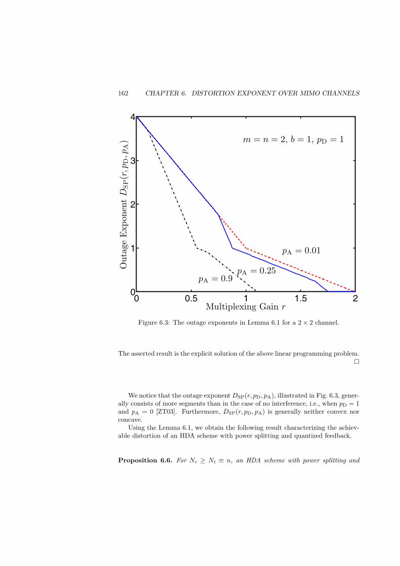
162 CHAPTER 6. DISTORTION EXPONENT OVER MIMO CHANNELS
0 0.5 1 1.5 20
1
2
3
4
Multiplexing Gain r
Out
age
Exp
onen
tD
SP(r
,pD,p
A) m = n = 2, b = 1, pD = 1
pA = 0.9pA = 0.25
pA = 0.01
Figure 6.3: The outage exponents in Lemma 6.1 for a 2× 2 channel.
The asserted result is the explicit solution of the above linear programming problem.
We notice that the outage exponentDSP(r, pD, pA), illustrated in Fig. 6.3, gener-ally consists of more segments than in the case of no interference, i.e., when pD = 1and pA = 0 [ZT03]. Furthermore, DSP(r, pD, pA) is generally neither convex norconcave.
Using the Lemma 6.1, we obtain the following result characterizing the achiev-able distortion of an HDA scheme with power splitting and quantized feedback.
Proposition 6.6. For Nr ≥ Nt ≡ n, an HDA scheme with power splitting and

6.5. ACHIEVABLE DISTORTION EXPONENTS: HDA WITH POWERSPLITTING 163
feedback resolution K ≥ 2 can achieve a distortion exponent of
dHDA−POW−NPC−K(b) = sup0<r1,...,rK<n,0<p1,...,pK<1
min {
DSP(rK , 1, pK),br1 + p1,
br2 +DSP(r1, 1, p1) + max(p2 −
n− p1b − r1
1− 1bn
, p2 − 1 + r1 − (n− 1)(
1− p1bn
), 0),
. . .
brK +DSP(rK−1, 1, pK−1)
+ max(pK −
n− pK−1b − rK−1
1− 1bn
, pK − 1 + rK−1 − (n− 1)(
1− pK−1
bn
), 0)}
under a short-term power constraint, and
dHDA−POW−PC−K(b) = sup0<r1,...,rK<n,{pk<1+Dk−1}
min {
DK , br1 + p1,
br2 + max(
0, p2 − pD1, p2 −npD1 − p1
b − r11− 1
bn
, p2 − pD1 + r1 − (n− 1)(pD1 − p1
bn
))+D1,
. . .
brK + max(
0, pK − pDK−1, pK −npDK−1 − pK−1
b − rK−1
1− 1bn
pK − pDK−1
+rK−1 − (n− 1)(pDK−1 − pK−1
bn
))+DK−1
}
under a long-term power constraint. Herein DkΔ= DSP(rk, 1 + Dk−1, pk), pDk
Δ=1 +Dk−1 with D0
Δ= 0.
The pi’s herein refer to the SNR exponent of the power allocated to the analoglayer. In the short-term power constraint case, the digital layer has pD = 1 forall feedback indices. In the long-term constraint case, the power exponent of thedigital layer is denoted by pDk.
The proof of Proposition 6.6, deferred to Appendix 6.F, essentially follows thatof Proposition 6.4. The presence of more terms inside the max(·) is due to the factthat g(x) = (pD − x)+ − 1
bn (pA − x)+ is piece-wise linear in 0 < x < pD. We omita lower bound on the achievable distortion in the case Nt > Nr, which is similar toProposition 6.5.
Unlike the dimension splitting case, even numerically evaluating the distor-tion exponent in Proposition 6.6 is difficult due to the presence of the parameters

164 CHAPTER 6. DISTORTION EXPONENT OVER MIMO CHANNELS
0 2 4 6 8 100
1
2
3
4
Bandwidth ratio b
Dis
tort
ion
expo
nent
d
K = 1 (No CSIT)
K = 2 (1 bit)Perfect CSIT
Solid: Dimension splittingDotted: Power splittingDashed: Single-layer approach
Figure 6.4: Distortion exponent of different schemes over a 2× 2 channel. A short-term power constraint is assumed.
p1, . . . , pK . In the numerical section, we resorted to a grid search on the (p1, . . . , pK)space. This is of course prohibitive even for a moderate K.
The achievability of power-splitting schemes is much more difficult to analyzefor finite-length source and channel codes. The quantization error for a finite sourcevector length Ns is generally not Gaussian, making the analysis complicated. Evenif it were possible to replace the quantization error with i.i.d. Gaussian noise,then we still need to show the existence of channel codes with finite-length havingthe approximately universal property, taking the partially overlapping behavior ofthe system into account. This is a very difficult task even for a traditional no-interference model [TV06, EKP+06]. Finite-length coding analysis of the proposedscheme remains an interesting topic for future work.
6.6 Numerical Examples
We plot in Fig. 6.4 the achievable distortion of different schemes under a short-termpower constraint. As can be seen, even one bit of feedback information improves

6.6. NUMERICAL EXAMPLES 165
0 2 4 6 8 100
10
20
30
40
Bandwidth ratio b
Dis
tort
ion
expo
nent
d
Perfect CSIT
Perfect CSIT - Short-term
Solid: Dimension splittingDashed: Single-layer approach
K = 2
K = 3
Figure 6.5: Achievable distortion exponents of different schemes over a 4× 4 chan-nel. A long-term power constraint is assumed. The K-power-level upper bounds,marked by circles, are also plotted.
the performance significantly. For comparison, we also plot the performance of theoptimal joint source-channel rate allocation, see e.g., [HG05], (i.e., the single-layercoding scheme). For the sake of clarity, we recall here that a “single-layer” codingscheme is a scheme that for each feedback index I(H) = i allocates a power level Piand a channel coding rate Ri, and makes use of an all digital “tandem” code withsource coding rate bRi and channel coding rate Ri. This differs from the proposedHDA schemes that make use of hybrid digital-analog strategies for each value ofthe feedback index, and also from the upper bounds, for which we have assumed afinite and discrete set of power levels P1, . . . , PK but a continuum of tandem codingschemes such that the source coding rate can be made equal to the instantaneouschannel mutual information. Notice also that single-layer schemes can be obtainedas special cases of the proposed power-splitting HDA scheme by allocating no powerto the analog layer.
It is demonstrated in Fig. 6.5, where the distortion exponents over a 4 × 4channel are plotted, that temporal power control is instrumental in achieving a

166 CHAPTER 6. DISTORTION EXPONENT OVER MIMO CHANNELS
large distortion exponent in the high bandwidth ratio regime. For example, apartial power controlled system with a single bit of feedback outperforms a nopower control system with perfect CSIT by a wide margin for all b ≥ 5. In thescenarios considered, one can achieve performance very close to perfect-CSIT witha very coarse feedback resolution K. Recall however from Proposition 6.2 that theperformance gap between the finite-feedback case and the perfect-CSIT case growsas b increases, unless the feedback resolution also grows (logarithmically) with b.
In Fig. 6.5 the upper- and lower bounds corresponding to the same value of Kwill eventually coincide as the bandwidth ratio becomes large. This is because eventhe simple single-layer coding scheme can achieve the upper bound DUB–PC–K(b)as b→∞:
limb→∞dSL–PC–K(b) = lim
b→∞supr1,...,rK
min (br1, br2 +D1, . . . , brK +DK−1,DK)
≥ limb→∞
min(K∑k=1
(mn)k,DK
(∑Kk=1(mn)k
b
))
=K∑k=1
(mn)k
where the inequality is obtained by choosing r1 = · · · = rK =∑K
k=1(mn)k
b and thelast equality is due to limε↓0DK(ε) =
∑Kk=1(mn)k.
6.7 Conclusion
We have studied the end-to-end distortion exponent of single-user fading MIMOchannels with limited feedback. One remarkable conclusion is that the optimizedsingle-layer approach achieves performance very close to that of the HDA schemeseven for a moderate feedback resolution. Our single-layer results also suggest thatin a practical scenario, the schemes with a library of source and channel codes thatadapt rate and power based on partial feedback is a practically sound approach,provided that power and rate control are jointly optimized. This highlights theimportance of a careful cross-layer design in multimedia transmission over wirelessfading channels. Finding joint-source channel coding schemes with properly de-signed feedback links that achieve the upper bound dUB−PC−K(b) for any feedbackresolution K (similar to the HDA scheme with dimension splitting over a SISOchannel) remains an open problem.
6.A. PARTIAL-CSIT UPPER BOUND 167
Appendices for Chapter 6
6.A Partial-CSIT Upper Bound
Proof of Proposition 6.2The upper bound is obtained by assuming that perfect CSIT is available, but thesystem is only allowed to use K power levels.
The set of all channel realizations that use the same power level is referred toas a quantization region. Let Rk, pk ≥ 1 be the kth quantization region and thecorresponding SNR exponent of the power level. Without loss of generality, assume1 = p1 < · · · < pK < pK+1 =∞. The long-term power constraint leads to
supαn1∈Rk
pk −n∑i=1
(2i− 1 +m− n)αi ≤ 1,
or equivalently
infαn1∈Rk
n∑i=1
(2i− 1 +m− n)αi ≥ pk − 1.
Achievable rates and therefore distortion exponents are non-decreasing functionsof power. Thus the optimal kth quantization region simply consists of all channelrealizations where the highest power level can be applied without violating thepower constraint:
Rk ={αn1 ≥ 0 : pk − 1 ≤
n∑i=1
(2i− 1 +m− n)αi < pk+1 − 1}. (6.12)
Let dk be the distortion exponent over the region Rk. Then dUB−PC−K(b) =sup min(d1, . . . , dK) where the supremum is over all parameters used to characterizethe Rk’s. First consider
dK = infαn1∈RK
n∑i=1
(b(pK − αi)+ + (2i− 1 +m− n)αi
). (6.13)
A relaxed version of (6.13) has a simple solution:
infαn1≥0
n∑i=1
[b(pK − αi)+ + (2i− 1 +m− n)αi
]= pKdNPC−∞(b). (6.14)
Recall that dNPC−∞(b) is the distortion exponent for the ideal-CSIT case withoutpower control. With b > m− n+ 1, the optimizers α∗i of (6.14) satisfy
n∑i=1
(2i− 1 +m− n)α∗i ≥ (m− n+ 1)pK > pK − 1

168 CHAPTER 6. DISTORTION EXPONENT OVER MIMO CHANNELS
meaning that they belong to RK . Thus solutions of (6.13) and (6.14) coincide, and
dK = pKdNPC−∞(b).
Now consider the region R1, with
d1 = infαn1≥0
n∑i=1
[b(1− αi)+ + (2i− 1 +m− n)αi
]
s.t.n∑i=1
(2i− 1 +m− n)αi < p2 − 1.(6.15)
Consider a relaxed version of (6.15)
infαn1≥0
n∑i=1
[b(1− αi)+ + (2i− 1 +m− n)αi
], (6.16)
with solution αrlx1 = · · · = αrlx
J = 1, αrlxJ+1 = · · · = αrlx
n = 0 where
JΔ= max j ∈ {1, . . . , n} s.t. b ≥ 2j − 1 +m− n.
Note that∑ni=1(2i − 1 +m − n)αrlx
i = D(n − J, 1), i.e., the diversity gain corre-sponding to multiplexing gain n − J . Recall that we only consider b ≥ m − n + 1so that J is well defined.
If the minimum of (6.15) coincides with that of (6.16) then d1 = dNPC−∞(b) <dK . Thus dUB−PC−K(b) ≤ dNPC−∞(b), leading to a contradiction, as dNPC−∞(b)can be seen as dUB−PC−K(b) with one power level K = 1. The optimizers of (6.15)therefore must have the form α∗1 = · · · = α∗I−1 = 1, 0 ≤ α∗I < 1, α∗I+1 = · · · = α∗n =0 for some I ∈ {1, 2, . . . , J} so that the constraint in (6.15) is active, i.e.,
n∑i=1
(2i− 1 +m− n)α∗i = p2 − 1
Let r1 =∑ni=1(1−α∗i )+ = n− I + 1−α∗I ∈ (n− J, n) then d1 = br1 +D(r1, 1) and
p2 = D(r1, 1) + 1.Repeating this argument over R2, . . . ,RK−1 and optimizing over r1, . . . , rK−1
lead to the asserted result.
Some InterpretationsEven though the bounding technique of Proposition 6.2 considers a system thatuses K power levels and a continuum of multiplexing gains (rates), we are ableto characterize the upper bound using only K − 1 variables r1, . . . , rK−1. Thevariables rk’s can be interpreted as the multiplexing gains on the boundaries of the

6.A. PARTIAL-CSIT UPPER BOUND 169
quantization regions in the feedback link. To see that, note that by definition ofrk, the power exponents pk can be recursively characterized via rk via the relation:
pk = 1 +D(rk−1, pk−1) (6.17)
with the convention r0 = 0, p0 = 0. Inserting these into the definition of thequantization region k (6.12), we have
Rk ={αn1 ≥ 0 : D(rk−1, pk−1) <
n∑i=1
(2i− 1 +m− n)αi < D(rk, pk)}.
Now consider the dual problem of the diversity gain problem
infαn1≥0
n∑i=1
(pk − αi)+ s.t.n∑i=1
(2i− 1 +m− n)αi < D(rk, pk),
which has minimum rk. We conclude that
infαn1∈Rk
n∑i=1
(pk − αi)+ = rk.
That is, when applying a power in the order of SNRpk to any channel realizationin Rk, a multiplexing gain of at least rk can be achieved.
Similarly, by considering
supαn1≥0
n∑i=1
(pk−1 − αi)+ s.t.n∑i=1
(2i− 1 +m− n)αi > D(rk−1, pk−1)
we have
supαn1∈Rk
n∑i=1
(pk−1 − αi)+ = rk−1.
That is, all channel realizations in Rk, when excited by a power of order SNRpk−1 ,cannot support the multiplexing gain rk−1 (resulting in an outage event with respectto power SNRpk−1 and rate rk−1 log SNR). This is consistent with (6.17) becausethe probability that the channel realization belongs to Rk is given by the outageprobability
Pr(αn1 ∈ Rk) .= SNR−D(rk−1,pk−1),
and thus the power exponent
pk = 1 +D(rk−1, pk−1)
can be applied over Rk without violating the long-term power constraint.

170 CHAPTER 6. DISTORTION EXPONENT OVER MIMO CHANNELS
0 1 2
2
6
10
14
r1
(1 + D(r1, 1))dNPC−∞(b)
br1 + D(r1, 1)
n − J = 1
b = 1.5
Figure 6.6: Computation of the bound DUB-PC−K(b) over a 2×2 channel, feedbackresolution K = 2. Case 1: J = 1.
Computation of dUB-PC−K(b)
Since dUB-PC−K(b) is an upper bound, finding the global optimum of the maximinin Proposition 6.2 is a critical task. In this section, we discuss some difficultieswhen computing this bound and give a conjecture on the optimal solution.
We first illustrate the K-level upper bound by studying a specific example.Consider a MIMO 2× 2 channel with feedback resolution K = 2. By definition wehave
dUB-PC−2 = supr1∈[n−J,n)
min {(1 +D(r1, 1))dNPC−∞(b), br1 +D(r1, 1))} (6.18)
for b ≥ m− n+ 1 = 1, where
D(r1, 1) ={
4− 3r1 if r1 ∈ (0, 1),2− r1 if r1 ∈ [1, 2).

6.A. PARTIAL-CSIT UPPER BOUND 171
0 1 20
10
20
r1
(1 + D(r1, 1))dNPC−∞(b)
br1 + D(r1, 1)
n − J = 0
b = 5
Figure 6.7: Computation of the bound DUB-PC−K(b) over a 2×2 channel, feedbackresolution K = 2. Case 2: J = 2.
and the upper bound without power control is given by [CN05]
dNPC−∞(b) =
⎧⎪⎨⎪⎩
2b if b ∈ [0, 1),b+ 1 if b ∈ [1, 3),4 otherwise.
We plot in Figs. 6.6 and 6.7 the two component functions in (6.18) and their point-wise minimum. The problem is clearly a nonconvex optimization. The parameterJ is b-dependent, in particular J = 1 for b < 3 and J = 2 for b ≥ 3.
For J = 1, due to the constraint r1 > n − J = 1, the optimum is given bythe intersection between the two linear segments (the intersection always exists),leading to dUB-PC−K(b) = (3b−1)(b+1)
2b . The constraint r1 > n − J = 1 essentiallyremoves all the segments of the piecewise linear function br1 +D(r1, 1) that have anegative slope.
For J = 2 or b ≥ 3, br + D(r1, 1) is nondecreasing in b, and the optimum isagain given by the intersection of two piecewise linear functions. Because of thepiecewise linearity, we need to distinguish between the case when the optimizer r∗1

172 CHAPTER 6. DISTORTION EXPONENT OVER MIMO CHANNELS
is in (0, 1] and when it is in (1, 2). We eventually obtain
dUB-PC−K(b) =
⎧⎪⎨⎪⎩
(3b−1)(b+1)2b if b ∈ [1, 3),
12b−4b+3 if b ∈ [3, 7),
20b−12b+9 if b ∈ [7,∞).
Unfortunately, computing dUB-PC−K(b) for a higher feedback resolution K ismuch more complicated. The component functions in the maximin are generallynot concave, thus their point-wise minimum is not a concave function. Interestingly,in all the cases that we observed, equating all K components always gives a uniquesolution in (n−J, n)K , and this intersection yields the largest value of the point-wiseminimum (as confirmed by a grid search). This suggests that the global optimummay indeed be achieved by the intersection of all K component functions. Howeverwe have not been able to prove this conjecture analytically.
The computation of other achievable bounds in this chapter also gives rise tosimilar difficulties. However, finding the global one for an achievable bound ofthe maximin form is less critical because any local optimum still serves as a lowerbound.
6.B Derivation of K-level Upper Bound and AchievableDistortion Exponent for SISO Channels
Partial-CSIT Upper BoundWe need to prove the equality (6.9). For m = n = 1, we have dNPC−∞(b) = 1,∀b ≥ 1. Furthermore, from the diversity-multiplexing results in Chapter 3 we have
D1 = D(r1) = 1− r1,D2 = D(r2, 1 +D1) = 2− r1 − r2,· · ·
DK−1 = K − 1− r1 − . . .− rK−1.
Applying these results to Proposition 6.2 gives
dUB−PC−K(b) = sup0<r1,...,rK−1<1
min (1 +K − 1− r1 − . . .− rK−1,
br1 + 1− r1,br2 + 2− r1 − r2,· · ·brK−1 +K − 1− r1 − . . .− rK−1) .
The point-wise minimum of a family of affine functions is concave [BV04]. Theglobal optimum of the maximin in this particular case is obtained when all the

6.B. DERIVATION OF K-LEVEL UPPER BOUND AND ACHIEVABLEDISTORTION EXPONENT FOR SISO CHANNELS 173
exponents are equal, provided that the solution of such a system of equations existsand is strictly inside (0, 1)K−1. Balancing the K terms inside the brackets yields
rK−1 = 1b,
rK−2 = 1b
+ b− 1brK−1 = 1
b+ b− 1b2,
· · ·
r1 = 1b
+ b− 1b2
+ . . .+ (b− 1)K−2
bK−1 = 1−(b− 1b
)K−1
.
We indeed have rk ∈ (0, 1),∀k. Finally, for a SISO channel with b ≥ 1 we have
dUB−PC−K(b) = 1 + (b− 1)[
1−(b− 1b
)K−1]
= b− b(
1− 1b
)K.
Achievable Distortion ExponentIn this section, we show that the exponent (6.11) is achievable for the SISO case.Consider a simple source-channel coding system with optimized rate allocationwhere the transmitter allocates a fixed rate ri log SNR for all α1 ∈ Ri where ri themaximum multiplexing gain that all channel realizations in Ri can support, i.e.
ri+1 log SNR > log(1 + SNRpi−α1
) ≥ ri log SNR,∀α1 ∈ Ri.For such a system, we can achieve a distortion exponent of
min(d1, d2, . . . , dK , dout)
where di is the distortion exponent over Ri and dout is the outage exponent. Hereinoutage is the event
log(1 + SNRpK−α1) < rK log SNR.
We then have p1 = 1, Pr(α1 ∈ R1) .= SNR0, and Pr(α1 /∈ R1) .= SNR−D(r1,1) =SNR−(1−r1). The average exponent over R1 has the same exponent as
SNR−br1 Pr(α1 ∈ R1) .= SNR−br1 .
Hence d1 = br1. Then the power level in R2 is in the order of
SNRp2 .= SNRPr(α1 ∈ R2)
.= SNR2−r1
and the average exponent over R2 has the same exponent as
SNR−br2 Pr(α1 ∈ R2) .= SNR−br2−D(r1,1) = SNR−br2−(1−r1).

174 CHAPTER 6. DISTORTION EXPONENT OVER MIMO CHANNELS
This gives d2 = br2 + 1− r1. Repeating the arguments yields
d3 = br3 + (1 + 1− r1)− r2 = br3 + 2− r1 − r2,· · ·
dK = brK +K − 1− r1 − · · · − rK−1.
Finally the outage exponent is given by
dout = D(rK , pK) = K − r1 − · · · − rK .Imposing d1 = · · · = dK = dout gives
rK = 1b+ 1
rK−1 = 1b+ 1 + b
b+ 1rK = 1b+ 1 + b
(b+ 1)2
· · ·
r1 = 1b+ 1 + b
(b+ 1)2 + · · ·+ bK−1
(b+ 1)K = 1−(b
b+ 1
)K.
Finally,
dSL–PC–K = b− bK+1
(b+ 1)K ,
which is (6.11) that we want to prove.
6.C Proof of Proposition 6.3
We need the following lemma.
Lemma 6.2 (Linear lower bounds on the D-M curves). Define Dk(r)Δ= D(r, 1 +
Dk−1(r)) where D0(r) Δ= 0,∀r, then
DK(r) ≥[
(m− n+ 1)K−1∑k=0
[(m− n+ 1)n]k]
(n− r).
Proof. The lower bound is obtained by extending the last (rightmost) segment ofthe D-M curve Dk(r) to the entire (0, n). We claim that the last segment of Dk(r)is given by
(m− n+ 1)L−1∑k=0
[(m− n+ 1)n]k(n− r)
and show that by induction.

6.C. PROOF OF PROPOSITION 6.3 175
For k = 1 the claim holds. Assume the claim holds for k = l ≥ 1, we will showthat it also holds for l+ 1. For simplicity, first denote κ = (m−n+ 1)n. Note thatfor r ∈ [(n−1)p, np) we have D(r, p) = (m−n+1)(np− r). Thus, the last segmentof Dl+1(r) is given by
(m− n+ 1)(n(1 +Dl(r))− r) = κ+ κ(m− n+ 1)l−1∑k=0
κk(n− r)− (m− n+ 1)r
= κl∑k=0
κk −l∑k=0
κk(m− n+ 1)r
=[
(m− n+ 1)l∑k=0
κk
](n− r).
It now remains to show that Dk(r) (which is piecewise linear) is convex so thatthe extension of the last segment serves as a lower bound. To that end, we willshow that the negative slope of Dk(r) is non-increasing in r.
To see that, recall from [ZT03] an important property of D(r, p): If we letI = � rp� then the negative slope ofD(r, p) at r is (m−I)(n−I)−(m−I−1)(n−I−1),independent of p. Note that (m−I)(n−I)− (m−I−1)(n−I−1) = m+n−1−2Iis a decreasing function of I.
Now for any k, let I(x) = x1+Dk−1(x) . If x < y then Dk−1(x) > Dk−1(y), thus
I(x) = x
1 +Dk−1(x) < I(y) = y
1 +Dk−1(y) .
This means the negative slope of D(x, 1 + Dk−1(x)) is decreasing in x, and thusthe piece-wise linear function Dk(x) = D(x, 1 +Dk−1(x)) is convex, ∀k.
We now prove Proposition 6.3. Recall that we assume m > 1 throughout.
Proof of SufficiencyAssume
limb→∞
b
[(m− n+ 1)n]K(b) = 0. (6.19)
Again consider an optimized single-layer coding system. Note that the distortionexponent of such a system with K(b) levels of feedback is given by
dSL–PC–K(b)(b) = sup0<r1,...,rK(b)<n
min(br1, br2 +D1, . . . , brK(b) +DK(b)−1,DK(b)
).
Choosing r1 = r2 = · · · = rK(b) = n − Cb[(m−n+1)n]K(b) where C is a finite positive
constant specified later, we obtaindSL–PC–K(b)
b≥ min
(n− Cb
[(m− n+ 1)n]K(b) ,DK(b)(r1)b
).

176 CHAPTER 6. DISTORTION EXPONENT OVER MIMO CHANNELS
Using the lower bound in Lemma 6.2, we have
DK(b)(r1)b
≥ m− n+ 1b
[(m− n+ 1)n]K(b) − 1(m− n+ 1)n− 1
Cb
[(m− n+ 1)n]K(b) .
Note that (m− n+ 1)n > 1 since m > 1. Choosing
C = n (m− n+ 1)n− 1(m− n+ 1)
and taking the limit b→∞, we then obtain
limb→∞dSL–PC–K(b)
b≥ min
(n, n lim
b→∞[(m− n+ 1)n]K(b) − 1
(m− n+ 1)n]K(b)
)= n,
given that (6.19) holds.
Proof of NecessityAssume there exists at least one scheme that is asymptotically efficient, then wemust have η = n. From the definition of dUB−PC−K(b), for b > m+ n− 1 we have
dUB−PC−K(b) ≤ sup0<r1,...,rK(b)<n
mn(1 +DK(b)−1)
= mn(
1 +mn+ . . .+ (mn)K(b)−1)
= mn
mn− 1
((mn)K(b) − 1
).
Note that mn > 1 because m > 1. Thus
n = limb→∞dUB−PC−K(b)
b
≤ mn
mn− 1 limb→∞
(mn)K(b)
b,
leading tolimb→∞
b
(mn)K(b) ≤m
mn− 1 ,
which is the asserted condition.Note that in the m = n = 1 case, we can use exactly the same arguments but
the results slightly change because∑K(b)k=1 (mn)k = K(b). In particular we obtain a
sufficient conditionlimb→∞
b
K(b) = 0
and a necessary conditionlimb→∞
b
K(b) ≤ 1.

6.D. PROOF OF PROPOSITION 6.4 177
This is redundant because it is known from a direct investigation in Section 6.3that the exact necessary and sufficient condition is (6.10), i.e.,
limb→∞
(1− 1b
)K(b)
= 0.
6.D Proof of Proposition 6.4
Short-term Power ConstraintBefore proceeding to the main proof, we note that when transmitting an i.i.d. zero-mean unit-variance Gaussian vector of length Nt ≤ Nr, the MMSE averaged overa subset A of channel matrices is given by∫
AMMSE(H)f(H)dH .=
∫A
tr(INr + SNRHHH)−1
f(H)dH
=∫A
n∑i=1
11 + SNR1−αi f(α
n1 )dαn1 .
The dominating terms then have a negative SNR exponent of
inf{αn1≥0}∩A
[(1− α1)+ +
n∑i=1
(2i− 1 +m− n)αi]. (6.20)
This fact will be used later in the proof.Let n > r1 > · · · > rK > 0 be the multiplexing gains of the digital part and
let d1, . . . , dK be the distortion exponents over the K corresponding quantizationregions. Then the scheme can achieve a distortion exponent of
min(dout, d1, . . . , dK),
where dout is the outage exponent.By definition, we have
dout = D(rK , 1).
We now compute d1. Let σ2e1.= SNR−de1 be the variance of the quantization error
(i.e., the difference between the source vector s and the output of the tandemencoder)
SNR−d1 .= SNR−de1SNR−mmse1 = SNR−(de1+mmse1).
Since the analog part occupies only a fraction of the block, the effective bandwidthratio is
T − Nsn
Ns= b− 1
n

178 CHAPTER 6. DISTORTION EXPONENT OVER MIMO CHANNELS
The resulting distortion exponent is obtained from the rate-distortion limit asfollows. We have σ2
e1 = exp(−Rs), with the source coding rate Rs satisfyingRsNs = (T − Ns/n)r1 log SNR. It follows that the variance of the error has anSNR exponent given by
de1 =(b− 1n
)r1.
Furthermore, solving (6.20) with the non-outage region
A = R1 ={αn1 :
n∑i=1
(1− αi)+ ≥ r1},
we readily obtain the optimizers α∗1 = · · · = α∗n = 0 and thus
mmse1 = 1.
This leads tod1 = de1 + mmse1 =
(b− 1n
)r1 + 1.
We next compute d2 = de2 + mmse2. Again we have
de2 =(b− 1n
)r2.
To compute mmse2, we solve the optimization (6.20) with
A = R2 ={αn1 : r2 ≤
n∑i=1
(1− αi)+ < r1
}.
With this A, the optimizers α∗i of (6.20) always coincide with those of the problem:
inf{αn1≥0}∩A
n∑i=1
(2i− 1 +m− n)αi.
But the above minimum is exactly the diversity gain D(r1, 1). This means that∑ni=1(1−α∗i )+ = r1, and α∗1 = 1 if r1 ≤ n−1 and α∗1 = n−r1 if r1 ≥ n−1, leading
tommse2 = (r1 + 1− n)+ +D(r1, 1).
Finally
d2 =(b− 1n
)r2 +D(r1, 1) + (r1 + 1− n)+.
Repeating the above steps for d3, . . . , dK and optimizing over the rate r1, . . . , rKgives the claimed result.

6.D. PROOF OF PROPOSITION 6.4 179
Long-term Power ConstraintThe proof follows exactly the same arguments as those of the short-term powerconstraint case. The main difference comes from the fact that with a long-termpower constraint, a power in the order Pk
.= SNRPr(H∈Rk) can be applied to the region
Rk.Let d1, . . . , dK be the distortion exponents corresponding to R1, . . . ,RK . We
still haved1 = de1 + mmse1 =
(b− 1n
)r1 + 1.
As for
R2 ={αn1 :
n∑i=1
(1− αi)+ < r1,
n∑i=1
(p2 − αi)+ ≥ r2},
we have de2 =(b− 1
n
)r2. The power level applied to this region P2
.= SNR1+D(r1,1) =SNR1+D1 ≡ SNRp2 and thus
mmse2 = inf{αn1≥0}∩R2
[(1 +D1 − α1)+ +
n∑i=1
(2i− 1 +m− n)αi]
= D1 + (r1 + 1− n)+ +D1,
which eventually leads to
d2 =(b− 1n
)r2 + 2D1 + (r1 + 1− n)+.
At the (possibly locally) optimal rate allocation, impose d1 = d2 or(b− 1n
)r1 + 1 =
(b− 1n
)r2 + 2D1 + (r1 + 1− n)+. (6.21)
The function 2D1 + (r1 + 1−n)+ is monotonically non-increasing in r1 thus 2D1 +(r1 + 1− n)+ > 1 for 0 < r1 < n. If r2 ≥ r1 then (6.21) cannot be satisfied. Thusr2 < r1, and therefore D2 = D(r2, 1 +D1) > D(r1, 1 +D1) > D(r1, 1) = D1.
Now consider
R3 ={αn1 :
n∑i=1
(1 +D1 − αi)+ < r2,n∑i=1
(1 +D2 − αi)+ ≥ r3},
where we have
mmse3 = inf{αn1≥0}∩R3
[(1 +D2 − α1)+ +
n∑i=1
(2i− 1 +m− n)αi]
= (1 +D2 − (1 +D1) + (r2 − (n− 1)(1 +D1))+)+ +D2
= 2D2 −D1 + (r2 + (1− n)(1 +D1))+,

180 CHAPTER 6. DISTORTION EXPONENT OVER MIMO CHANNELS
where the second equality is due to the fact that the optimizer α∗1 = n(1 +D1)− r2if r2 > (n− 1)(1 +D1) and α∗1 = 1 +D1 otherwise, and the last equality is due toD1 < D2. This leads to
d3 =(b− 1n
)r3 + 2D2 −D1 + (r2 + (1− n)(1 +D1))+.
Repeating the arguments leads to the asserted result.
6.E Proof of Proposition 6.5
The proof follows the same pattern of the proof of Proposition 6.4. To avoidrepetition, we only present the computation of a bound to the MMSE exponent,which is the key difference from Proposition 6.4.
To further simplify the presentation, consider the short-term power constraint,and a feedback resolution K = 2. Let H be the n × n sub-matrix channel usedfor the transmission of the analog part. Let μi = SNR−βi be the correspondingeigenvalues. In the first region R1, MMSE(H ∈ R1) .= SNR−mmse1 where
mmse1 = infβn1≥0∩R1
(1− β1)+ +n∑i=1
(2i− 1)βi
≥ infβn1≥0
(1− β1)+ +n∑i=1
(2i− 1)βi
= 1.
This leads tod1 =
(b− 1n
)r1 + 1.
Consider R2 = {αn1 : r2 ≤∑ni=1(1− αi)+ < r1}. The event that log det(INr +
SNRHHH) < R implies that log det(INr +SNRHHH) < R due to the monotonicityof log det(·) on the semi-definite cone. Equivalently, the event αn1 ∈ R2 also implies∑ni=1(1− βi)+ < r1. Let
R2 ={βn1 :
n∑i=1
(1− βi)+ < r1
}⊃ R2,
then MMSE(H ∈ R2) .= SNR−mmse2 where
mmse2 = infβn1≥0∩R2
(1− β1)+ +n∑i=1
(2i− 1)βi
≥ infβn1≥0∩R2
(1− β1)+ +n∑i=1
(2i− 1)βi
= (1 + r1 − n)+ +Dnn(r1, 1).

6.F. PROOF OF PROPOSITION 6.6 181
This leads tod2 =
(b− 1n
)r2 +Dnn(r1, 1) + (1 + r1 − n)+.
6.F Proof of Proposition 6.6
Consider a short-term power constraint and the following index mapping, which ischaracterized indirectly via αn1 ≥ 0,
I (αn1 ) =
⎧⎪⎨⎪⎩K if
∑ni=1 (1− αi)+ − 1
bn (pK − αi)+ < rK ,
k : rk−1 +∑ni=1
1bn (pk−1 − αi)+ >
∑ni=1 (1− αi)+
≥ rk +∑ni=1
1bn (pk − αi)+ otherwise.
We first compute the distortion exponent over the quantization region R1 cor-responding to I = 1
d1 = br1 + mmse1.
Notice that there is no loss in bandwidth since the analog part is superimposedonto the digital codeword, resulting in the quantization error (at the output of thetandem encoder) of order SNR−br1 . The analog part however can only use a powerin the order of SNRp1 , thus (similarly to (6.20))
mmse1 = inf(αn1≥0)∩R1
{(p1 − α1)+ +
n∑i=1
(2i− 1 +m− n)αi}
where
R1 ={αn1 :
n∑i=1
[(1− αi)+ − 1
bn(p1 − αi)+
]≥ r1}.
This optimization gives mmse1 = p1, ∀r1 ∈(0, n− p1
b
)and thus d1 = br1 + p1.
Now consider
R2 ={αn1 :
n∑i=1
[(1− αi)+ − 1
bn(p1 − αi)+
]< r1,
n∑i=1
[(1− αi)+ − 1
bn(p2 − αi)+
]≥ r2}
and
mmse2 = inf(αn1≥0)∩R2
{(p2 − α1)+ +
n∑i=1
(2i− 1 +m− n)αi}.

182 CHAPTER 6. DISTORTION EXPONENT OVER MIMO CHANNELS
Since the term (p2 − α1)+ can only reduce the weight corresponding to α1, theoptimizers α∗i ’s of the above optimization coincide with these of
inf(αn1≥0)∩R2
n∑i=1
(2i− 1 +m− n)αi,
meaning that
α∗1 =
⎧⎪⎪⎪⎪⎨⎪⎪⎪⎪⎩
1 if r1 < (n− 1)(1− p1
bn
)1− r1 + (n− 1)
(1− p1
bn
)if (n− 1)
(1− p1
bn
) ≤ r1< (n− 1)
(1− p1
bn
)+ 1− p1,
n− p1b −r1
1− 1bn
if (n− 1)(1− p1
bn
)+ 1− p1 ≤ r1 < n
(1− p1
bn
)and that
∑ni=1(2i− 1 +m− n)α∗i = DSP(r1, 1, p1). This eventually leads to
mmse2 = max(
0, p2 − 1 + r1 − (n− 1)(
1− 1bn
), p2 −
n− p1b − r1
1− 1bn
)+DSP(r1, 1, p1)
and d2 = br2 + mmse2.Continuing this line of arguments, we obtain the achievable distortion exponent
of Proposition 6.6 under a short-term power constraint. The exponent for the long-term power constraint case can be derived in a completely similar manner.

Chapter 7
Distortion Exponent over RelayChannels
This chapter continues on the distortion exponent problem, with a new focus onthe relay channels with limited feedback. Building upon results from Chapters 4and 6, we show that under a short-term power constraint, combining a simplefeedback scheme with separate source and channel coding outperforms the bestknown no-feedback strategies even with only a few bits of feedback information.Partial power control is shown to be instrumental in achieving a very fast decayingaverage distortion, especially in the regime of high bandwidth ratios. Performancelimitation due to the lack of full CSI at the destination feedback quantizer is alsoinvestigated, where the degradation in terms of the distortion exponent is shown tobe significant. However, even in such restrictive scenarios, using partial feedbackstill yields distortion exponents superior to any no-feedback schemes.
7.1 Introduction
Despite the large amount of work in the literature addressing various performancemeasures in cooperative systems, many challenging problems remain open. Oneparticular scenario is the transmission of a source over a slow fading channel. Inthis problem the separation theorem [CT91] does not hold when the channel stateinformation is not fully known at the transmitter. Indeed, even if the transmitterin a relay channel knows the full CSI, the optimal strategy for source transmissionis still unknown, as the capacity of a completely general relay channel is a longstanding open problem.
In the context of source–channel coding over relay channels, various protocolsare proposed and their achievable distortion exponents are analyzed in [GE07b]under the assumption that the source and the relay do not have any knowledge oftheir corresponding forward channel gains. However, for many practical scenarios,limited channel state feedback is present at the transmitter side, allowing for partial
183

184 CHAPTER 7. DISTORTION EXPONENT OVER RELAY CHANNELS
S D
R
h
h1h2
I
I
Figure 7.1: System model. Note that in the feedback model of Section 7.3, we haveI = I(h, h1, h2). On the other hand, the feedback index in Section 7.4 does notdepend on h1, i.e., I = I(h, h2)
.
rate and/or power adaptation.This chapter studies the asymptotic performance of the average end-to-end dis-
tortion over a three-node single-antenna relay channel in the presence of partialCSIT. We derive upper bounds on the optimal distortion exponent of any possiblerelaying and feedback strategy, given the number of feedback levels. For the achiev-ability part, we exclusively focus on the decode-and-forward strategy [LTW04]. Weshow that even with the separation of source and channel coding, partial rate con-trol allows for an improved performance over the best layering schemes in [GE07b].Thus the separation of source–channel coding provides an effective yet simple so-lution in practical systems, even if some optimality may be lost. Temporal powercontrol with limited CSIT provides additional gains which cannot be obtained byany no-feedback system. Finally, upper bounds and achievable bounds for the caseof channel states partially known at the destination are derived. Even in such a re-strictive scenario, using partial rate and power control still provides superior gains,especially in the low spectral efficiency regime.

7.2. SYSTEM MODEL 185
7.2 System Model
Consider the complex baseband model of a frequency-nonselective half-duplex fad-ing relay channel, depicted in Fig. 7.1. The three single-antenna nodes in thesystems are the source, the relay, and the destination. The channel is assumed tobe slowly fading, i.e., the channel gains are constant during a fading block con-sisting of T channel uses, but changes independently from one block to the next.We exclusively consider the case when a transmission codeword spans a single fad-ing block to study the gain from spatial cooperation. The channel is assumed tobe statistically symmetric. In particular, h, h1, and h2 are i.i.d. complex Gaus-sian random variables with zero mean and unit variance. That is, we consider aquasi-static Rayleigh fading scenario. Assume perfect CSI at the receiver of eachcommunication link in the system, and perfect synchronization.
We consider individual power constraints at the source and at the relay. Since wedeal with partial-CSIT systems, both short-term and long-term power constraintsare considered, as in Chapter 4.
At the source, an i.i.d. memoryless Gaussian source produces Ns complex sym-bols s every T time instant. The source symbols are assumed to have zero meanand unit variance. Let b = Ns
T be the channel bandwidth to source bandwidth ratio(bandwidth ratio).
At each SNR, let the mean squared error between the source vector and thereconstructed vector be
Δ = 1Ns
E[‖s− s‖22
]where the expectation is over the randomness of the source symbols, the noise andthe channel gains. We consider a sequence of schemes at increasingly high SNR,and obtain a sequence of Δ indexed by SNR. Completely similarly to Chapter 6,the system is then said to achieve a distortion exponent of d if
Δ .= SNR−d.
We are interested in characterizing the distortion exponent d as a function of thebandwidth ratio b. This provides a coarse (in the limit of asymptotically high SNR)tradeoff between spectral efficiency (via b) and distortion (represented by d), givinguseful insight into the performance of different source transmission schemes.
7.3 Distortion Exponents with Channel State Feedback
In this section we consider the scenario where the channel states h, h1 and h2 arefully known at the destination. The destination then maps the tuple of channelstates into an integer index I(h, h1, h2) ∈ {1, . . . ,K} and broadcasts this index toboth the source and the relay via a noiseless zero-delay dedicated feedback link (cf.Fig. 7.1).

186 CHAPTER 7. DISTORTION EXPONENT OVER RELAY CHANNELS
Upper Bounds to the Distortion Exponent
We begin by deriving relevant upper bounds to the distortion exponent that can beachieved by any source–channel coding scheme over the relay channel of interest.
First we have the cooperative transmitters upper bound, obtained by lettingthe source and the relay fully cooperate resulting in a MISO 2× 1 channel:
dUBMISO–NPC(b) = min(b, 2)
under a short-term power constraint; and
dUBMISO–PC(b) = b
under a long-term power constraint. Recall that the proof for the no power controlcase can be found in [GE08, CN07], and the power control case is presented inChapter 6. Both bounds assume perfect CSIT. Note that for b < 1, even using asimple HDA scheme in [CN07] over a SISO channel can achieve the MISO upperbound. The regime of b < 1 is therefore not of our interest.
For the power control case, in Chapter 6 an upper bound for the MISO channelwith K power levels is given. For b < 2, the upper bound for a MISO channelwith K levels of feedback trivially coincides with that of the perfect-CSIT case, i.e.dUB–K
MISO–PC(b) = b, ∀K. Otherwise, we have:
Proposition 7.1. For b ≥ 2, the distortion exponent of a 2×1 MISO channel withK levels of feedback is upper-bounded by
dUB–KMISO–PC(b) =
4b− 2(b− 2)(b−22b)K−1
4 + (b− 2)(b−22b)K−1 .
Note that the upper bound dUB–KMISO–PC(b) is given in the form of a general maximin
problem in Chapter 6. To obtain the explicit form in Proposition 7.1, the proofin Appendix 7.A deviates from that in Chapter 6, expressing the upper bound inthe form of an optimization problem with respect to the power levels instead of themultiplexing gains.
Rewriting
dUB–KMISO–PC(b) = 2K+1bK − 2(b− 2)K
2K+1bK−1 + (b− 2)K
we readily obtain
Corollary 7.1.
limb→∞dUB–K
MISO–PC(b) = 2K+1 − 2 =K∑k=1
2k.

7.3. DISTORTION EXPONENTS WITH CHANNEL STATE FEEDBACK 187
This is consistent with the limiting results in multiple-antenna channels, ob-tained by an indirect approach in Chapter 6. In short, dUB–K
MISO–PC(b) equals to themaximal diversity gain of the 2 × 1 channel with K feedback levels, because atlow spectral efficiency, even if the multiplexing gain can be made close to zero, theaverage distortion of the system is still outage-limited.
Achievable Distortion Exponents without Power ControlIn this section, we derive certain achievable bounds to the optimal distortion ex-ponent over relay channels with feedback. We exclusively study decode–forwardrelaying [LTW04] as this strategy naturally fits into our quantized feedback frame-work.
In short, the DF protocol that we consider consists of two communicationphases. Phase 1 uses βT channel uses with β ∈ (0, 1). The source in Phase 1encodes a message m to a codeword of length βT and transmits. The relay at-tempts to decode m based on its received signal in Phase 1. In Phase 2, if thesource–relay link is not in outage the relay re-encodes m and transmits. Otherwisethe relay outputs nothing. The source may transmit (1 − β)T additional symbolsin Phase 2, in which case we have a non-orthogonal scheme; or it may remain silent(in orthogonal schemes). The destination decodes based on the received signals inboth phases.
Notice that for a given multiplexing gain, the numbers of channel uses allocatedto Phase 1 and Phase 2 in DF relaying can be optimized over (which we often referto as dimension allocation) so as to maximize the diversity gain. The diversitygain of DF relaying with optimized dimension allocation is given in the followinglemma. This is a natural extension of Proposition 4.1, which deals with the no-power control case (i.e., when the transmit power is SNR1, to the power controlcase). The proof is relatively similar to that of Proposition 4.1, and thus omitted.
Lemma 7.1. Let the transmit power at both the source and the relay be SNRpwhere p ≥ 1, then the outage exponent of DF relaying with optimized dimensionallocation is
DDFO (r, p) =
{2p− 3r if r < p3 ,2p(p−r)p+r otherwise.
for orthogonal schemes, and
DDFNO(r, p) =
{2p− 3+
√5
2 r if r < 3−√52 p,
(2p−r)(p−r)p otherwise
for non-orthogonal schemes. The optimal allocation of the available channel usesis
β∗(r, p) ={
23 if r < p3 ,p+r2p otherwise
188 CHAPTER 7. DISTORTION EXPONENT OVER RELAY CHANNELS
in the orthogonal case, and
β∗(r, p) ={√
5−12 if r < 3−√5
2 p,p
2p−r otherwise
in the non-orthogonal case.
For convenience, we denote the diversity gain in the no power control case asDDF
O (r) Δ= DDFO (r, 1) and DDF
NO(r) Δ= DDFNO(r, 1). Similarly β∗(r) Δ= β∗(r, 1).
The proposed feedback scheme works as follows. For brevity we only describethe orthogonal case, as the non-orthogonal scheme is based on a similar idea.
The system is equipped with a library of K tandem encoders [MP02], i.e. Kpairs of source encoder and channel encoder, with channel code rates {ri log SNR}bits per channel use, where 1 > r1 > · · · > rK > 0. Herein K is the number offeedback levels, also known as the feedback resolution. Upon receiving the indexI(h, h1, h2) = i fed back from the destination, the source node encodes the sourcesymbols with the tandem code whose channel code rate is ri log SNR. Given I = i,orthogonal DF relaying with optimal allocation β∗(ri) will be used.
Let μO(h, h1, h2; r) be the mutual information of the orthogonal scheme giventhe channel states h, h1, h2 and a certain multiplexing gain r, i.e.
μO(h, h1, h2; r) Δ=
⎧⎪⎨⎪⎩β∗(r) log
(1 + |h|2SNR
)if log
(1 + |h1|2SNR
)< r log SNR
β∗(r) ,
β∗(r) log(1 + |h|2SNR
)+ (1− β∗(r)) log
(1 + |h2|2SNR
),
otherwise.
The destination employs the index mapping
I(h, h1, h2) ={K if μO(h, h1, h2; rK) < rK log SNR,max i ∈ {1, . . . ,K} s.t. μO(h, h1, h2; ri) ≥ ri log SNR otherwise.
(7.1)That is, the destination informs the source node to use the largest channel code ratepossible in the library of codes so that the transmission will not be in outage. This isequivalent to using the quantizer with the highest resolution possible to encode thesource. In case the channel is in a too bad condition and no reliable communicationis possible with any rate in the library, we can send back an arbitrary index (whichis set to K in (7.1)) without changing the results.
We are now ready to state the following achievable distortion exponents. Theproof is deferred to Appendix 7.B.
Proposition 7.2. Under a short-term power constraint at both the source and therelay, the proposed orthogonal scheme can achieve the distortion exponent
dKO–NPC(b) = sup1>r1>···>rK>0
min(DDF
O (rK), br1, . . . , brK +DDFO (rK−1)
).

7.3. DISTORTION EXPONENTS WITH CHANNEL STATE FEEDBACK 189
The non-orthogonal scheme can achieve
dKNO–NPC(b) = sup1>r1>···>rK>0
min(DDF
NO(rK), br1, . . . , brK +DDFNO(rK−1)
).
Unfortunately, the optimization problems in Proposition 7.2 are not convex,because DDF
O (r) and DDFNO(r) are not concave functions. However, for sufficiently
high b, these maximin problems can be reduced to convex ones. In such cases, wecan find the closed-form expression of the distortion exponents in Proposition 7.2.
Corollary 7.2. For b ≥ 6
dKO–NPC(b) = 2(b3)K+1 − b3(b3)K+1 − 1
.
For b ≥ 3 +√
5
dKNO–NPC(b) = 2
(3−√5
2 b)K+1
− 3−√52 b(
3−√52 b)K+1
− 1.
Proof. We need the following lemma. The proof is straightforward and thus omit-ted.
Lemma 7.2. Let (x∗1, . . . , x∗K) be the solutions to the system of linear equations
bx1 = bx2 + γ − θx1 = · · · = bxK + γ − θxK−1 = γ − θxKwhere γ > 0, θ > 0 are real parameters then
Δ Δ= bx∗1 = γ(bθ
)K+1 − bθ(bθ
)K+1 − 1
and
x∗k = Δ− γb
1− ( θb )K1− θb
+(θ
b
)K−1γ
b.
We now prove Corollary 7.2. Consider only the orthogonal case. Since dKO–NPC(b)≤ 2, it suffices to consider r1 such that br1 ≤ 2 or r1 ≤ 2
b . But 2b <
13 , ∀b > 6, thus
rK < · · · < r1 < 13 and DDF
O (rk) = 2− 3rk, ∀k. In this case, the maximin problemfinding dKO–NPC(b) is of the form
sup2b>r1>···>rK>0
min {2− 3rK , br1, br2 + 2− 3r1, . . . , brK + 2− 3rK−1} .

190 CHAPTER 7. DISTORTION EXPONENT OVER RELAY CHANNELS
0 1 2 3 4 50
1
2
Bandwidth Ratio b
Dis
tort
ion
Exp
onen
td
K = 4
K = 2
MISO Upperbound
K = 1
Solid: Non-orthogonalDashed: Orthogonal
Figure 7.2: Achievable distortion exponents with different feedback resolution K.A short-term power constraint is assumed.
This is a convex optimization, since the pointwise minimum of linear functionsis concave. Equating all the terms and applying Lemma 7.2 yields the claimeddKO–NPC(b). It can then be verified that with this dKO–NPC(b), the linear constraints2b > r1 > · · · > rK > 0 are fulfilled.
For b outside the range specified in Corollary 7.2, we obtain achievable boundsby equating all the terms inside the mininum of Proposition 7.2 and solving thesesystems of equations numerically.
We plot in Fig. 7.2 the achievable distortion exponents of both orthogonal andnon-orthogonal schemes without power control. Clearly, a few bits of feedbackinformation provides an excellent performance, even with the very simple single-layer coding scheme that we consider. Indeed, over a certain range of b, the proposedfeedback schemes with K as low as 4 (2 bits) outperform even the best known no-feedback strategies in [GE07b], which require a very high complexity in terms ofinfinitely many code layers (cf. Fig. 7.3). We also observe that in this low feedbackrate regime, the effect of adding one bit of CSIT is much more pronounced thanswitching from orthogonal to non-orthogonal schemes. Thus from a practical point
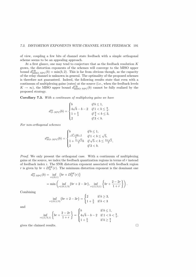
7.3. DISTORTION EXPONENTS WITH CHANNEL STATE FEEDBACK 191
of view, coupling a few bits of channel state feedback with a simple orthogonalscheme seems to be an appealing approach.
At a first glance, one may tend to conjecture that as the feedback resolution Kgrows, the distortion exponents of the schemes will converge to the MISO upperbound dUB
MISO–NPC(b) = min(b, 2). This is far from obvious though, as the capacityof the relay channel is unknown in general. The optimality of the proposed schemesis therefore not guaranteed. Indeed, the following results state that even with acontinuum of multiplexing gains (rates) at the source (i.e., when the feedback levelsK → ∞), the MISO upper bound dUB
MISO–NPC(b) cannot be fully realized by theproposed strategy.
Corollary 7.3. With a continuum of multiplexing gains we have
d∞O–NPC(b) =
⎧⎪⎪⎪⎨⎪⎪⎪⎩b if b ≤ 1,4√b− b− 2 if 1 < b ≤ 9
4 ,
1 + b3 if 9
4 < b ≤ 3,2 if 3 < b.
For non-orthogonal schemes
d∞NO–NPC(b) =
⎧⎪⎪⎪⎨⎪⎪⎪⎩b if b ≤ 1,−b2+6b−1
4 if 1 < b ≤ √5,1 + 3−√5
2 b if√
5 < b ≤ 3+√
52 ,
2 if 3 < b.
Proof. We only present the orthogonal case. With a continuum of multiplexinggains at the source, we index the feedback quantization regions in terms of r insteadof feedback index i. The SNR distortion exponent associated with feedback regionr is given by br +DDF
O (r). The minimum distortion exponent is the dominant one
d∞O–NPC(b) = infr∈(0,1)
{br +DDF
O (r)}
= min(
infr∈(0,1/3)
{br + 2− 3r}, infr∈(1/3,1)
{br + 2− 2r
1 + r
}).
Combining
infr∈(0,1/3)
{br + 2− 3r} ={
2 if b ≥ 3,1 + b
3 if b < 3and
infr∈(1/3,1)
{br + 2− 2r
1 + r
}=
⎧⎪⎨⎪⎩b if b ≤ 1,4√b− b− 2 if 1 < b < 9
4 ,
1 + b3 if b ≥ 9
4
gives the claimed results.

192 CHAPTER 7. DISTORTION EXPONENT OVER RELAY CHANNELS
0 1 2 3 4 50
1
2
Bandwidth Ratio b
Dis
tort
ion
Exp
onen
td
MISO Upperbound
Solid: Non-orthogonalDashed: Orthogonal
HDA+DDFBS
Figure 7.3: Achievable distortion exponents of the proposed schemes with a con-tinuum of multiplexing gains (no power control). The distortion exponent of thebroadcast strategy (BS) with mixed DF and direct transmission [GE07b], and thatof the HDA scheme with dynamic DF [GE07b], are also plotted, both in the limitof infinitely many layers.
In Fig. 7.3, the distortion exponents achieved by using a continuum of ratesat the source are plotted. Clearly both studied schemes cannot achieve the MISOupper bound over an intermediate range of the bandwidth ratio b. We also seethat even in the high feedback resolution regime, the non-orthogonal scheme stilldisplays some advantage over the orthogonal one for certain values of b. On a finalnote, the best known source–channel coding schemes without CSIT in [GE07b],namely the HDA scheme coupled with dynamic DF and the broadcast strategywith mixed DF and direct transmission, do not approach d∞O–NPC(b) even whenequipped with infinitely many code layers, as illustrated in Fig. 7.3.
Achievable Distortion Exponents with Power ControlWe now relax the power constraint, allowing the source and the relay to controltheir transmit power based on channel state feedback from the destination. Thescheme that we study is described as follows. Again, we only describe the orthogonal

7.3. DISTORTION EXPONENTS WITH CHANNEL STATE FEEDBACK 193
scheme.The system is equipped with a library of K tandem codes with channel code
rates {ri log SNR} where 1 > r1 > · · · > rK > 0 and a power codebook consistingof K predetermined power levels {P1 < · · · < PK}. The destination broadcastsa common feedback index I(h, h1, h2) to both the source and the relay. Uponreceiving I = i, the source and the relay properly scale their transmit codewords sothat each individual transmit power is Pi. Given I = i, DF relaying with optimaldimension allocation is used.
The following index mapping is used by the destination
I(h, h1, h2) ={
1 if μO(h, h1, h2;PK , rK) < rK log SNR,max i ∈ {1, . . . ,K} s.t. μO(h, h1, h2;Pi, ri) ≥ ri log SNR otherwise.
Similarly to the no power control case, μO(h, h1, h2;Pk, rk) is the mutual informa-tion (given that power Pk is used). In essence, the scheme first tries the highestcode rate possible. If that fails, lower code rates in conjunction with higher powerwill be attempted.
Proposition 7.3. With power control at both source and relay, the proposed or-thogonal scheme can achieve
dKO–PC(b) = sup1>r1>...>rK>0
min(DKO , br1, br2 +D1
O, . . . , brK +DK−1O)
where DkOΔ= DDF
O (rk, 1 +Dk−1O ), with D0
O = 0.The non-orthogonal scheme can achieve
dKNO–PC(b) = sup1>r1>...>rK>0
min(DKNO, br1, br2 +D1
NO, . . . , brK +DK−1NO)
where DkNOΔ= DDF
NO(rk, 1 +Dk−1NO ), with D0
NO = 0.
The proof closely follows that of Proposition 7.2 and is thus omitted. Thepresence of the terms DkO and DkNO is due to the recursive nature of the DMT withquantized CSIT.
We demonstrate the potential of power control with limited feedback in Fig. 7.4.As can be seen, the gain of using (even partial) power control is significant. Theeffect is particularly pronounced in the high bandwidth ratio regime. For example,an orthogonal scheme using only two levels of power control provides a betterperformance than any no power control strategy as long as b ≥ 3.7. Note that theachievable bounds however fall short of getting close to the corresponding K-levelupper bounds, leaving room for future improvement.
In the limit of large bandwidth ratios, the distortion exponents of both orthog-onal and no-orthogonal schemes converge to the upper bound dUB–K
MISO–PC(b) for anygiven K:

194 CHAPTER 7. DISTORTION EXPONENT OVER RELAY CHANNELS
0 1 2 3 4 50
1
2
3
4
5
Bandwidth Ratio b
Dis
tort
ion
Exp
onen
td
K = 3Solid: Non-orthogonalDashed: Orthogonal
K = 2
K = 2
K = 3
K-level Upperbound
Figure 7.4: Achievable distortion exponents with power control and different K.The corresponding K-level upper bounds are also plotted.
Corollary 7.4.
limb→∞dKO–PC(b) = lim
b→∞dUB–K
NO–PC(b) =K∑k=1
2k.
Proof. It suffices to consider the orthogonal case. By choosing r1 = · · · = rK =
rΔ= min
(∑K
k=12k
b , 1)
we obtain
limb→∞dKO–PC(b) ≥ lim
b→∞min(DKO , br, br +D1
O, . . . , br +DK−1O)
= limb→∞
min(DKO , br
)=K∑k=1
2k.
The last equality is due to limb→∞ r = 0, and the fact that DKO →∑Kk=1 2k when
the multiplexing gain tends to zero.

7.4. DISTORTION EXPONENTS WITH A RESTRICTED FEEDBACKQUANTIZER 195
7.4 Distortion Exponents with a Restricted FeedbackQuantizer
In practice, while the destination can learn h and h2 via training, acquiring accurateknowledge about the source–relay channel gain h1 at the destination is a difficulttask. This motivates the studies presented in this section where we consider thescenario that h1 is unknown to the feedback quantizer at the destination. Toderive a tighter upper bound than DUB–K
MISO (b), we let the relay and the destinationfully cooperate, resulting in a 1 × 2 channel with K levels of feedback. Howeverthe feedback quantizer depends only on a single scalar gain, since the destinationquantizer does not know h1 by assumption. Computing an upper bound to thedistortion exponent over such a channel with restricted feedback quantizer gives thefollowing. The proof is deferred to Appendix 7.C.
Proposition 7.4. Assume that the index mapping at the destination does not knowthe source-relay gain h1. With power control at both the source and the relay, andK feedback levels from the destination, the distortion exponent is upper-bounded by
dUB–KPC (b) = b− (b− 2)K
bK−1 .
In the limit of large bandwidth ratios b, i.e. at very low spectral efficiency, wehave
Corollary 7.5. For any K ≥ 2
limb→∞dUB–K
PC (b) = 2K.
Comparing the above limit with that of dUB–KMISO–PC(b), we can see that not know-
ing h1 incurs a large degradation in the distortion exponent. In such scenarios, therate at which the end-to-end distortion decays to zero will increase much slower(as a function of the feedback resolution K) than in the case of full-CSI at thedestination. This is due to the degradation of the diversity gain in this scenario,cf. Chapter 4.
We now describe a particular scheme operating under such a constraint on theCSI at the destination and study its achievable distortion exponents.
The proposed index mapping is
I(h, h2) ={K if log(1 + |h|2PK−1) < rK−1 log SNR,max i ∈ {1, . . . ,K − 1} s.t. log(1 + |h|2Pi) ≥ ri log SNR otherwise.
The source uses direct transmission for =1, . . . ,K − 1, i.e. β1 = · · ·βK−1 = 1 anduses (either orthogonal or non-orthogonal) DF with rate rK log SNR and optimizedfraction β∗K(rK) when I = K. That is, the proposed scheme rarely makes use ofthe relay.
196 CHAPTER 7. DISTORTION EXPONENT OVER RELAY CHANNELS
Proposition 7.5. If b ∈ {b :(b2 − 3
) ( 1+bb
)K−1> b2 − b} then the proposed
orthogonal scheme can achieve
dKO–PC(b) =(2b+ 3)
( 1+bb
)K−1 − 2b− 1(2 + 3
b
) ( 1+bb
)K−1 − 1.
If b ∈ {b :(b2 − 3
) ( 1+bb
)K−1 ≤ b2 − b} then dKO–PC(b) = −B−√B2−4AC2A where
A = 2(1 + b)2K−1 − 3bK−1(1 + b)K + b2K−1,
B = b(3bK − 4(1 + b)K
) ((1 + b)K−1 − bK−1)− (b+ 2)bK−1(1 + b)K−1,
andC = 2b2
((1 + b)K − bK) (bK−2 + (1 + b)K−1 − bK−1) .
For non-orthogonal schemes, if
b ∈{b :(b2 − (3−
√5)b− 5 +
√5
2
)(1 + bb
)K−1
> b2 − 5−√52 b
}
then
dKNO–PC(b) =
(2b+ 3+
√5
2
) ( 1+bb
)K−1 − 2b−√
5−12(
2 + 3+√
52b
) ( 1+bb
)K−1 − 1
If b ∈{b :(b2 − (3−√5)b− 5+
√5
2
) ( 1+bb
)K−1 ≤ b2 − 5−√52 b}
then dKNO–PC(b) =−B−√B2−4AC
2A where
A = b2K − 3bK(1 + b)K + (2b+ 1)(1 + b)2K−1,
B = −3b2K+1 − 2b(2b+ 1)(1 + b)2K−1 + (7b2 + 5b− 1)bK(1 + b)K−1,
andC = b2
((1 + b)K − bK) ((2b+ 1)(1 + b)K−1 − (2b− 1)bK−1) .
In Fig. 7.5, we plot the achievable distortion exponents with restrictive feedbackquantizers. Even these restricted feedback schemes yield significant gains over a no-CSIT system, but they stay short of getting close to the upper bound except at thehigh spectral efficiency regime (very small b) and the very low spectral efficiencyregime (very high b - not plotted herein). We can also conclude that the high-SNRgain of non-orthogonal schemes is negligible.
Finally, for completeness, we state the asymptotic optimality of both schemesin the high-b regime. The proof is similar to that of Corollary 7.4.
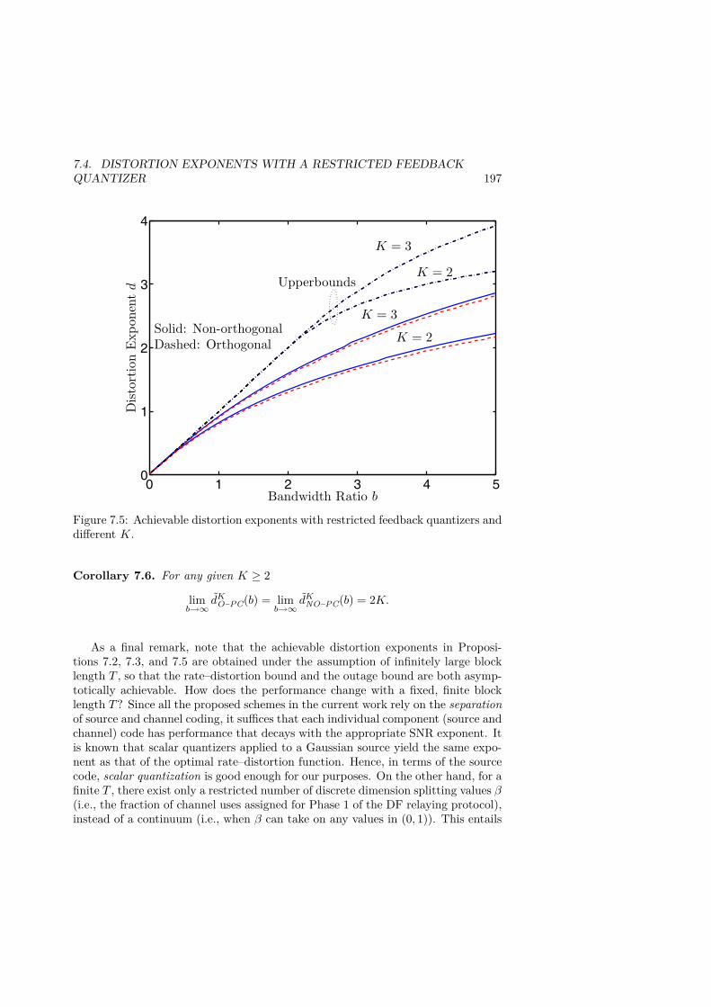
7.4. DISTORTION EXPONENTS WITH A RESTRICTED FEEDBACKQUANTIZER 197
0 1 2 3 4 50
1
2
3
4
Bandwidth Ratio b
Dis
tort
ion
Exp
onen
td Upperbounds
Solid: Non-orthogonalDashed: Orthogonal
K = 3
K = 2
K = 2
K = 3
Figure 7.5: Achievable distortion exponents with restricted feedback quantizers anddifferent K.
Corollary 7.6. For any given K ≥ 2
limb→∞dKO–PC(b) = lim
b→∞dKNO–PC(b) = 2K.
As a final remark, note that the achievable distortion exponents in Proposi-tions 7.2, 7.3, and 7.5 are obtained under the assumption of infinitely large blocklength T , so that the rate–distortion bound and the outage bound are both asymp-totically achievable. How does the performance change with a fixed, finite blocklength T? Since all the proposed schemes in the current work rely on the separationof source and channel coding, it suffices that each individual component (source andchannel) code has performance that decays with the appropriate SNR exponent. Itis known that scalar quantizers applied to a Gaussian source yield the same expo-nent as that of the optimal rate–distortion function. Hence, in terms of the sourcecode, scalar quantization is good enough for our purposes. On the other hand, for afinite T , there exist only a restricted number of discrete dimension splitting values β(i.e., the fraction of channel uses assigned for Phase 1 of the DF relaying protocol),instead of a continuum (i.e., when β can take on any values in (0, 1)). This entails

198 CHAPTER 7. DISTORTION EXPONENT OVER RELAY CHANNELS
a certain loss in the achievable error exponent of the channel code compared to theoutage exponent. Consequently, for any finite T the achievable distortion exponentsare generally less than those obtained for infinite T presented in this work, due tothe channel coding part. This loss however asymptotically (and rather quickly, asstudied in Chapter 4) vanishes as T increases.
7.5 Conclusion
We have investigated the problem of rate and power allocation using partial CSITto maximize the decay rate of the end-to-end expected distortion in a single-antennarelay channel. Even a few levels of rate control allows a simple separate source andchannel coding scheme to outperform the best known complex no-feedback strate-gies. The performance can be further improved with an appropriate partial powercontrol policy. Our results suggest that combining simple relaying schemes withlow-rate channel state feedback can be an effective approach for the transmissionof analog sources over cooperative channels.
Appendices for Chapter 7
7.A Proof of Proposition 7.1
Consider a 1 × 2 slow fading channel with i.i.d. zero-mean unit-variance complexGaussian channel gains a1, a2. Let α = − log(|a1|2+|a2|2)
log SNR . To obtain an upperbound to the distortion exponent, we assume perfect CSIT so that the transmittercan perform perfect rate adaptation. However the transmitter is constrained to useonly K power levels.
Let Pk.= SNRpk be the K power levels at the transmitter, with 1 = p1 < · · · <
pK < pK+1 =∞. We refer to the set of all α’s that are mapped to a certain powerlevel Pk as the kth quantization region Rk. We only consider α ≥ 0 as the regiona < 0 has a probability measure that exponentially decays in SNR and thus doesnot affect the SNR exponent of interest [ZT03]. The long-term power constraintleads to ∫
RkSNRpkf(α)dα ≤ SNR
where f(α) is the p.d.f. of α. Some standard large-deviation arguments [ZT03]then lead to
supα∈Rk
{pk − 2α} ≤ 1
Since the end-to-end distortion is a decreasing function of transmit power, we con-clude that
Rk ={α ≥ 0 : pk − 1
2 ≤ α < pk+1 − 12
}.

7.A. PROOF OF PROPOSITION 7.1 199
Because the transmitter can do perfect rate adaptation, the multiplexing gainof the transmit rate corresponding to a channel state α is the same as that oflog(1 + SNRpk−α). Assume codes achieving the rate-distortion function, the aver-age distortion over Rk is then
Δk.=∫Rk
2−b log(1+SNRpk−α)f(α)dα
Thus for a fixed set of power levels, the distortion exponent over Rk is given by
dk = infα∈Rk
{b(pk − α)+ + 2α
}.
Since pK+1 = ∞, over RK the optimization readily gives dK = 2pK with theoptimizer α∗ = pK . For any k < K,
dk ={
2pk if pk < pk+1−12 ,
bpk − (b−2)(pk+1−1)2 if pk ≥ pk+1−1
2 .
However, since d = min(d1, . . . , dK), the case dk = 2pk is not of interest, otherwise2pk < dK = 2pK meaning that adding the quantization region RK is redundant.Thus we only consider pk ≥ pk+1−1
2 , and optimize the power levels to obtain
DUB–KMISO–PC(b) = sup
p2,...,pK
min(
2pK , bp1 − b− 22 p2 + b− 2
2 , . . . ,
bpK−1 − b− 22 pK + b− 2
2
)s.t. 2p1 ≥ p2 − 1, . . . , 2pK−1 ≥ pK − 1, pK > · · · > p1.
Recall that p1 = 1. Since the functions inside the point-wise minimum are linearin pk’s, the solution to this maximin is the intersection of all the hyperplanes,i.e. at d1 = · · · = dK
Δ= d∗, provided that the intersection satisfies all the linearconstraints. We now have
pK = d∗
2 ,
pK−1 = d∗
b
(1 + b− 2
4
)− b− 2
2b ,
· · ·
pK−k = d∗
b
(1 + b− 2
2b + · · ·+(b− 2
2b
)k−1
+ (b− 2)k
2k+1bk−1
)−k∑i=1
(b− 2
2b
)i,
· · ·
p1 = d∗
b
(1− ( b−2
2b)K−1
b+22b
+ (b− 2)K−1
2KbK−2
)− b− 2
2b1− ( b−2
2b)K−1
b+22b
.

200 CHAPTER 7. DISTORTION EXPONENT OVER RELAY CHANNELS
Then, using the fact that p1 = 1, we have
d∗ =1 + b−2
b+2
(1− ( b−2
2b)K−1)
1−( b−22b )K−1
b+22
+ 12(b−22b)K−1
=4b− 2(b− 2)
(b−22b)K−1
4 + (b− 2)(b−22b)K−1 .
We can readily verify that with this d∗, the constraints 2pk ≥ pk+1 are all fulfilled.Thus dUB–K
MISO–PC(b) = d∗.
7.B Proof of Proposition 7.2
For brevity, we only present the orthogonal case. Let a = − log |h|2/ log SNR,α1 = − log |h1|2/ log SNR, α2 = − log |h2|2/ log SNR and thus we can write themutual information μO(a, α1, α2; r) = μO(h, h1, h2; r). The set of all channel statetuples that are mapped to an index I = k is referred to as quantization region Rk.Let the distortion exponent over Rk be dk. Define
Ok Δ= {a, α1, α2 ∈ R3+ : β∗(rk)(1− α1)+ < rk, β
∗(rk)(1− a)+ < rk}∪ {a, α1, α2 ∈ R
3+ : β∗(rk)(1− α1)+ ≥ rk,
β∗(rk)(1− a)+ + (1− β∗(rk))(1− α2)+ < rk}
which is essentially the asymptotic outage set conditioned on I = k.We readily have Pr(I = 1) .= SNR0 (intuitively, most channel uses do not result
in outage at high SNR), thus∫R1
2−b1r1 log SNRdadα1dα2.= SNR−br1 = SNR−d1 .
The exponent equality is due to an application of Bennett’s integral for high-ratevector quantization [NN95]. We next have
Pr(I = 2) = Pr(O2 ∩ O1) ≤ Pr(O1). (7.2)
Let Pr(I = 2) .= SNR−D2 then from (7.2): D2 ≥ DDFO (r1) = 2 − 2r1
β∗1 (r1) . Howeverby choosing a particular tuple a = 1 − r1
β∗1 (r1) + ε, α1 = a, α2 = 0 where ε > 0 isarbitrarily small, we then have
D2 = infO2∩O1
{a+ α1 + α2} ≤ 2− 2r1β∗1(r) + 2ε. (7.3)
For (7.3) to hold we have to show that (a, α1, α2) ∈ {O2 ∩ O1}
. To that end, noticethat β∗1(r1)(1 − a)+ = β∗1(r1)(1 − α1)+ = r1 − β∗1(r1)ε < r1 thus (a, α1, α2) ∈ O1(since both source–relay and source–destination links are in outage). In addition,

7.C. PROOF OF PROPOSITION 7.4 201
β∗2(r2)(1 − a)+ = β∗2(r2)(1 − α1)+ = β∗2(r2) r1β∗1 (r1) − β∗2(r2)ε > r2 for sufficiently
small ε. This is because
r
β∗(r) ={
3r2 if r < 1
3 ,2r
1+r otherwise.
is a monotonically increasing function of r, and thus for any r1 > r2 we have r1β∗1 (r1) >
r2β∗2 (r2) with strict inequality. Thus (a, α1, α2) ∈ O2 and (7.3) holds. Finally, letting
ε ↓ 0 we conclude that Pr(I = 2) .= SNR−DDFO (r1) and consequently d2 = b2r2 +
DDFO (r1). Continuing this line of arguments leads to the claimed results.
7.C Proof of Proposition 7.4
Let the relay and destination fully cooperate, resulting in a 1× 2 multiple-receiveantenna channel. Let a1, a2 be the two channel gains. Let α1 = − log |a1|2/ log SNRand α2 = − log |a2|2/ log SNR. The feedback index (thus the transmit power) onlydepends on a1 and not on a2. Thus we have supα1∈Rk {pk − α} ≤ 1 where Rk isthe kth quantization region. Then similarly to Appendix 7.A
Rk = {α1 : pk − 1 ≤ α1 < pk+1 − 1}.
The code rate associated with the channel state α1, α2 has the same multiplexinggain as log
(1 + SNRpk−α1 + SNRpk−α2
). Thus the distortion exponent over Rk is
dk = infα1∈Rk,α2≥0
bmax ((pk − α1), (pk − α2), 0) + α1 + α2.
We begin with RK where it is readily found that dK = 2pK . For k < K, it can beshown that
dk ={
2pk if pk < pk+1 − 1,b(pk − pk+1 + 1) + 2(pk+1 − 1) if pk ≥ pk+1 − 1.
Again the case dk = 2pk < 2pK is not of interest. Thus we end up with the maximinproblem
dUB–KPC (b) = sup
p2,...,pK
min (2pK , bp1 − (b− 2)p2 + b− 2, . . . ,
bpK−1 − (b− 2)pK + b− 2)s.t. p1 > p2 − 1, . . . , pK−1 > pK − 1, pK > . . . > p2 > p1 = 1.
This is again a convex optimization problem. We will find the intersection of allthe hyperplanes and verify that it satisfies all the linear constraints.

202 CHAPTER 7. DISTORTION EXPONENT OVER RELAY CHANNELS
Let d1 = · · · = dK Δ= d∗. We have
pK = d∗
2 ,
pK−1 = d∗
b
(1 + b− 2
2
)− b− 2b,
· · ·
pK−k = d∗
b
(1 + b− 2
b+ · · ·+
(b− 2b
)k−1
+ (b− 2)k
2bk−1
)−k∑i=1
(b− 2b
)i,
· · ·
p1 = d∗
b
(1− ( b−2
b
)K−1
2b
+ (b− 2)K−1
2bK−2
)− b− 2b
1− ( b−2b
)K−1
2b
But p1 = 1 thus we obtain
d∗ =1 +
(b−2)(
1−( b−2b )K−1)
21−( b−2
b )K−1
2 + (b−2)K−1
2bK−1
= 2 + (b− 2)(
1−(b− 2b
)K−1)
= b− (b− 2)K
bK−1 .
Again all the linear constraints are fulfilled with this d∗ and thus dUB–KPC (b) = d∗.
7.D Proof of Proposition 7.5
We only present the orthogonal case. Let pk be the SNR exponent of the powerlevels, i.e. Pk
.= SNRpk . Denote dk as the distortion exponent over the quantizationRk (the set of all channel state tuples that are mapped to I = k).
We have Pr(I = 1) .= SNR0 and thus d1 = br1. Then
Pr(I = 2) .= SNR−DSISO(r1,1).
Herein DSISO(r, p) = p − r is the diversity gain of a SISO channel correspondingto a multiplexing gain r and a transmit power SNRp. We then obtain d2 = br2 +DSISO(r1, 1) = br2 + 1− r1. The power applied to R2 thus have the SNR exponentp2 = 1+DSISO(r1, 1) = 1+1−r1 = 2−r1. Then Pr(I = 3) .= SNR−DSISO(r2,2−r1) =SNR−(2−r1−r2). We next have d3 = br3 + 2− r1 − r2.
Repeating the above arguments finally leads to dk = brk+k−1−r1−· · ·−rk−1,k = 1, . . . ,K − 1. Notice that due to construction, an outage event (the event that

7.D. PROOF OF PROPOSITION 7.5 203
the channel does not support the code rate) can only occur when I = K. Over theregion RK we have
dK = min(brK +K − 1− r1 − · · · − rK−1,DDFO (rK , pK)).
The optimization finding dKO–PC(b) can thus be written as
sup1>r1>...>rK>0
min (br1, br2 + 1− r1, br3 + 2− r1 − r2, . . . ,
brK +K − 1− r1 − · · · − rK−1,DDFO (rK ,K − r1 − . . .− rK−1)
)Note that this maximin is not a convex problem. However, since we are only
interested in an achievable distortion exponent, we can choose r1, . . . , rK to be thesolutions to
d∗ Δ= DDFO (rK ,K − r1 − . . .− rK−1) = br1 = br2 + 1− r1 = · · ·
= brK +K − 1− r1 − · · · − rK−1.
That is we find the point where all the terms are equal (and verify that such a pointexists). From brk−1 + k − 2 − r1 − · · · − rk−2 = brk + k − 1 − r1 − · · · − rk−1 weobtain
(1 + b)rk−1 = 1 + brk.This leads to the recursive relation
rk = 1 + bbrk−1 − 1
b
with the initial value r1 = d∗b . This recursion then gives
rk = 1−(
1 + bb
)k−1b− d∗b. (7.4)
We now consider the case when rK < pK3 = K−r1−...−rK−13 . From Lemma 7.1,
in this case we have DDFO (rk,K − r1− . . .− rK−1) = 2(K − r1− . . .− rK−1)− 3rK .
From (7.4) we have
K−1∑i=1ri = K − 1−
( 1+bb
)K−1 − 11b
b− d∗b
= K − 1−[(
1 + bb
)K−1
− 1]
(b− d∗).
This leads tod∗ = 2(K − r1 − . . .− rK−1)− 3rK
= 2(
1 +[(
1 + bb
)K−1
− 1]
(b− d∗))− 3(
1−(
1 + bb
)K−1b− d∗b
)
= −1 + (b− d∗)[
2(
1 + bb
)K−1
− 2 + 3b
(1 + bb
)K−1].

204 CHAPTER 7. DISTORTION EXPONENT OVER RELAY CHANNELS
Finally we obtain
d∗ =(2b+ 3)
( 1+bb
)K−1 − 2b− 1(2 + 3
b
) ( 1+bb
)K−1 − 1.
Recall that this happens iff rK < pK3 = K−r1−...−rK−13 , or
3− 3(
1 + bb
)K−1b− d∗b< 1 +
[(1 + bb
)K−1
− 1]
(b− d∗)
⇔ 2 < (b− d∗)[(
1 + bb
)K−1
− 1 + 3b
(1 + bb
)K−1]
⇔ 2 <(b− (2b+ 3)
( 1+bb
)K−1 − 2b− 1(2 + 3
b
) ( 1+bb
)K−1 − 1
)[(1 + 3b
)(1 + bb
)K−1
− 1]
⇔ (b2 − 3)(1 + b
b
)K−1
> b2 − b.
We now consider the remaining case rK ≥ pK3 , when Lemma 7.1 yields
d∗ = DDFO (rK , pK) = 2pK(pK − rK)
pK + rK.
Inserting (7.4) into the above expression gives
d∗(
2 +[b− 1b
(1 + bb
)K−1
− 1]
(b− d∗))
= 2(
1 +[(
1 + bb
)K−1
− 1]
(b− d∗))[(
1 + bb
)K− 1]
(b− d∗).(7.5)
This results in a quadratic equation of the form f(d∗) = 0 where f(d∗) Δ= Ad∗2 +Bd∗ + C with the coefficients A > 0, B, and C are given by Proposition 7.5. Us-ing (7.5), we can readily verify that f(b) < 0 and f(0) > 0, ∀b,K so that theequation f(d∗) = 0 has two real roots d∗1, d∗2 satisfying 0 < d∗1 < b < d∗2. This givesthe claimed result.

Chapter 8
Conclusion
8.1 Concluding Remarks
In this thesis, we have investigated the roles of partial CSIT in slow fading channels,including multiple-antenna and relaying systems. We considered many differentperformance metrics, leading to the introduction of radically different transmis-sion schemes. These schemes may utilize partial CSIT to adapt their transmissionpower, rate and even the time spent on each transmission phase. Analytical perfor-mance bounds are derived in each case, suggesting that very promising performanceimprovement may be achieved even if the CSIT is heavily quantized.
One important remark is that the impact of partial CSIT on fast and slowfading channels can be strikingly different, even if the performance criteria arequite similar. For instance, as we have seen from the study of expected rate,a couple of feedback bits can improve the expected rate over a scalar slow fadingchannel significantly. In contrast, the influence of quantized feedback on the ergodiccapacity of scalar fast fading channels is typically very small, especially at moderateand high SNR’s.
Another conclusion is the significant influence of rate and power adaptation overslow fading channels, even with coarsely quantized CSIT. In particular, with intel-ligent adaptation based on partial CSIT, the frame error probability of multiple-antenna and relaying systems can be made to decay extremely fast at high SNR.Remarkably, this improvement in reliability does not require any sacrifice in theasymptotic throughput. In relaying systems, we can additionally control the frac-tion of channel uses allocated to different transmission phases, which also leads tosignificant performance gains. This conclusion holds even when we transmit an ana-log source over slow fading channels and take the decaying rate of the end–to–endexpected distortion as performance measure.
205

206 CHAPTER 8. CONCLUSION
8.2 Future Work
Of course, many interesting questions still need answering, especially in relayingsystems. A particularly intriguing problem is to find relaying schemes that are D–M tradeoff optimal when the source and the relay have absolutely no CSIT. Recallthat with full CSIT, it is known that compress–and–forward relaying is optimalin the D–M tradeoff sense. Generalizing the results in the thesis to multiple-relaysystems with multiple-antenna nodes is also an important extension.
Designing and analyzing more sophisticated joint source–channel coding schemesthat can achieve the partial-CSIT upper bounds derived in the thesis is an interest-ing open problem. A better understanding of the effects of finite-length codes onthe end–to–end distortion exponent also requires more work. We may also thinkof an investigation on the distortion outage, i.e., the event that the end–to–enddistortion drops below an acceptable threshold.
A critical problem for practical wireless communication systems that adapt theirresources based on CSIT is the processing delay and the presence of noise in thefeedback link. Within the scope of this thesis, we have not paid enough attention tothese effects. Further work is needed before we can fully understand the detrimentaleffects that delayed and noisy feedback may cause to the D–M tradeoff and thedistortion exponent–bandwidth ratio tradeoff presented in the thesis. Designingintelligent schemes that are robust to noisy and delayed feedback would also be ofpractical relevance.
Apart from the expected rate maximization problem, we have mostly focusedon the asymptotically high SNR regime. While this asymptotic analysis provides a“clean” and compact characterization, thus giving useful insight into complicatedproblems, it does not necessarily give a complete picture about the system perfor-mance. In particular, the D–M tradeoff (as well as the distortion exponent analysis)totally ignores any constant gains in SNR, which are definitely important for anypractical communication systems. Therefore, a finer characterization of the systemperformance in a more practical range of the SNR would be a worthwhile and usefuldirection for future work.

Bibliography
[AES05] K. Azarian, H. El Gamal, and P. Schniter. On the achievable diversity-multiplexing tradeoffs in half-duplex cooperative channels. IEEETransactions on Information Theory, 51:4152–4172, December 2005.
[AEVZ02] E. Agrell, T. Eriksson, A. Vardy, and K. Zeger. Closest point searchin lattices. IEEE Transactions on Information Theory, 48:2201–2214,August 2002.
[AKSA06] N. Ahmed, M. A. Khojastepour, A. Sabharwal, and B. Aazhang. Out-age minimization with limited feedback for the fading relay channel.IEEE Transactions on Communications, 54:659–669, April 2006.
[Ala98] S. M. Alamouti. A simple transmitter diversity scheme for wirelesscommunications. IEEE Journal on Selected Areas in Communications,16:1451–1458, October 1998.
[BBT59] D. Blackwell, L. Breiman, and A. J. Thomasian. The capacity of aclass of channels. Ann. Math. Statist., 30:1229–1241, December 1959.
[BCT01] E. Biglieri, G. Caire, and G. Taricco. Limiting performance of block-fading channels with multiple antennas. IEEE Transactions on Infor-mation Theory, 47:1273–1289, May 2001.
[BGT93] C. Berrou, A. Glavieux, and P. Thitimajshima. Near Shannon limiterror-correcting coding and decoding: Turbo-codes. In Proc. IEEEInt. Conf. Communications, pages 1064–1070, May 1993.
[BNC06] K. Bhattad, K. Narayanan, and G. Caire. On the distortion exponentof some layered transmission schemes. In Proc. Asilomar Conf. Signals,Systems, Computers, pages 211–215, Pacific Grove, CA, October 2006.
[BPS98] E. Biglieri, J. Proakis, and S. Shamai (Shitz). Fading channels:Information-theoretic and communications aspects. IEEE Transactionson Information Theory, 44:2619–2692, October 1998.
[BR03] J.-C. Belfiore and G. Rekaya. Quaternionic lattices for space-time cod-ing. In Proc. Information Theory Workshop, pages 267–270, April 2003.
207

208 BIBLIOGRAPHY
[BRV05] J.-C. Belfiore, G. Rekaya, and E. Viterbo. The Golden code: A 2 ×2 full-rate space-time code with non-vanishing determinants. IEEETransactions on Information Theory, 51:1432–1436, April 2005.
[BSA02] S. Bhashyam, A. Sabharwal, and B. Aazhang. Feedback gain in multipleantenna systems. IEEE Transactions on Communications, 50:785–798,May 2002.
[BV04] S. Boyd and L. Vandenberghe. Convex Optimization. Cambridge Univ.Press, Cambridge, UK, 2004.
[CE79] T. M. Cover and A. A. El Gamal. Capacity theorems for the relay chan-nel. IEEE Transactions on Information Theory, 25:572–584, September1979.
[CN05] G. Caire and K. Narayanan. On the SNR exponent of hybrid digitalanalog space-time coding. In Proc. Annu. Allerton Conf. Communica-tion, Control, Computing, Monticello, IL, September 2005.
[CN07] G. Caire and K. Narayanan. On the distortion SNR exponent of hybriddigital-analog space time coding. IEEE Transactions on InformationTheory, 53:2867–2878, August 2007.
[Cov72] T. Cover. Broadcast channels. IEEE Transactions on InformationTheory, 18:2–14, January 1972.
[CPR03] J. Chou, S. S. Pradhan, and K. Ramchandran. Turbo and trellis-basedconstructions for source coding with side information. In Proc. DataCompression Conf., pages 33–42, Snowbird, UT, March 2003.
[CS99] G. Caire and S. Shamai (Shitz). On the capacity of some channels withchannel state information. IEEE Transactions on Information Theory,45:2007–2019, September 1999.
[CT91] T. M. Cover and J. A. Thomas. Elements of Information Theory. JohnWiley & Sons, New York, 1991.
[CTB99] G. Caire, G. Taricco, and E. Biglieri. Optimum power control overfading channels. IEEE Transactions on Information Theory, 45:1468–1489, July 1999.
[CX05] S. Cheng and Z. Xiong. Successive refinement for the Wyner-Ziv prob-lem and layered code design. IEEE Transactions on Signal Processing,53:3269–3281, August 2005.
[DZ98] A. Dembo and O. Zeitouni. Large Deviations Techniques and Applica-tions. Springer, New York, 1998.

209
[ECD04] H. El Gamal, G. Caire, and M. O. Damen. Lattice coding and decodingachieve the optimal diversity-multiplexing tradeoff of MIMO channels.IEEE Transactions on Information Theory, 50:968–985, June 2004.
[ECD06] H. El Gamal, G. Caire, and M. O. Damen. The MIMO ARQ channel:Diversity-multiplexing-delay tradeoff. IEEE Transactions on Informa-tion Theory, 52:3601–3621, August 2006.
[EG98] M. Effros and A. Goldsmith. Capacity definitions and coding strategiesfor general channels with receiver side information. In Proc. IEEE Int.Symp. Information Theory, page 39, August 1998.
[EKP+06] P. Elia, K. R. Kumar, S. A. Pawar, P. V. Kumar, and H.-F. Lu. Ex-plicit space-time codes achieving the diversity-multiplexing gain trade-off. IEEE Transactions on Information Theory, 52:3869–3884, Septem-ber 2006.
[EVAK06] P. Elia, K. Vinodh, M. Anand, and P. V. Kumar. D-MG tradeoff andoptimal codes for a class of AF and DF cooperative communicationprotocols. IEEE Transactions on Information Theory, November 2006.submitted for publication.
[FGW02] A. Forsgren, P. E. Gill, and M. H. Wright. Interior methods for non-linear optimization. SIAM Review, 44:525–597, October 2002.
[Fos96] G. J. Foschini. Layered space-time architecture for wireless commu-nication in a fading environment when using multi-element antennas.Technical report, Bell Labs. Tech. J., 1996.
[Gal62] R. Gallager. Low-density parity-check codes. IEEE Transactions onInformation Theory, 8:21–28, January 1962.
[Gal65] R. G. Gallager. A simple derivation of the coding theorem and someapplications. IEEE Transactions on Information Theory, 11:3–18, Jan-uary 1965.
[Gal68] R. G. Gallager. Information Theory and Reliable Communication. JohnWiley & Sons, New York, NY, 1968.
[GC97] A. J. Goldsmith and S.-G. Chua. Variable-rate variable-power MQAMfor fading channels. IEEE Transactions on Communications, 45:595–602, October 1997.
[GC98] A. J. Goldsmith and S.-G. Chua. Adaptive coded modulation for fadingchannels. IEEE Transactions on Communications, 46:595–602, May1998.
210 BIBLIOGRAPHY
[GE05] D. Gündüz and E. Erkip. Source and channel coding for quasi-staticfading channels. In Proc. Asilomar Conf. Signals, Systems, Computers,pages 18–22, Pacific Grove, CA, November 2005.
[GE07a] D. Gündüz and E. Erkip. Opportunistic cooperation by dynamic re-source allocation. IEEE Transactions on Wireless Communications,6:1446–1454, April 2007.
[GE07b] D. Gündüz and E. Erkip. Source and channel coding for cooperativerelaying. IEEE Transactions on Information Theory, 53:3454–3475,October 2007.
[GE08] D. Gündüz and E. Erkip. Joint source channel codes for MIMO blockfading channels. IEEE Transactions on Information Theory, 54:116–134, January 2008.
[GG92] A. Gersho and R. M. Gray. Vector Quantization and Signal Compres-sion. Kluwer Academic, Norwell, MA, 1992.
[GMW81] P. E. Gill, W. Murray, and M. H. Wright. Practical Optimization.Academic Press, London, UK, 1981.
[GØH05] A. Gjendemsjø, G. E. Øien, and H. Holm. Optimal power control fordiscrete-rate link adaptation schemes with capacity-approaching cod-ing. In Proc. IEEE Globecom, pages 3498–3502, November 2005.
[GS07] J. Giese and M. Skoglund. Space-time constellation design for par-tial CSI at the receiver. IEEE Transactions on Information Theory,53:2715–2731, August 2007.
[GV97] A. J. Goldsmith and P. P. Varaiya. Capacity of fading channels withchannel side information. IEEE Transactions on Information Theory,43:1986–1992, November 1997.
[HA04] M. O. Hasna and M.-S. Alouini. Optimal power allocation for relayedtransmissions over Rayleigh-fading channels. IEEE Transactions onWireless Communications, 6:1999–2004, November 2004.
[HG05] T. Holliday and A. J. Goldsmith. Optimizing end-to-end distortion inMIMO systems. In Proc. IEEE Int. Symp. Information Theory, pages1671–1675, Adelaide, Australia, September 2005.
[HH02] B. Hassibi and B. Hochwald. High-rate codes that are linear in spaceand time. IEEE Transactions on Information Theory, 48:18 04–1824,July 2002.
[HH03] B. Hassibi and B. M. Hochwald. How much training is needed inmultiple-antenna wireless links? IEEE Transactions on InformationTheory, 49:951–963, April 2003.

211
[HMT04] B. M. Hochwald, T. L. Marzetta, and V. Tarokh. Multiple-antennachannel hardening and its implications for rate feedback and scheduling.IEEE Transactions on Information Theory, 50:1893–1909, September2004.
[HT98] S. V. Hanly and D. N. C. Tse. Multiacess fading channels - Part II:Delay-limited capacities. IEEE Transactions on Information Theory,44:2816–2831, November 1998.
[HtB03] B. M. Hochwald and S. ten Brink. Achieving near-capacity on amultiple-antenna channel. IEEE Transactions on Communications,51:389–399, March 2003.
[HZ05] A. Høst-Madsen and J. Zhang. Capacity bounds and power allocationfor wireless relay channels. IEEE Transactions on Information Theory,51:2020–2040, June 2005.
[Jaf01] H. Jafarkhani. A quasi-orthogonal space-time block code. IEEE Trans-actions on Communications, 49:1–4, January 2001.
[JB04] E.A. Jorswieck and H. Boche. Channel capacity and capacity-range ofbeamforming in MIMO wireless systems under correlated fading withcovariance feedback. IEEE Transactions on Wireless Communications,3(5):1543–1553, September 2004.
[JG03] N. Jindal and A. Goldsmith. Capacity and optimal power allocationfor fading broadcast channels with minimum rates. IEEE Transactionson Information Theory, 49:2895–2909, November 2003.
[JG04] S. A. Jafar and A. Goldsmith. Transmitter optimization and optimalityof beamforming for multiple antenna systems. IEEE Transactions onWireless Communications, 3(4):1165–1175, July 2004.
[JO05] J. Jaldén and B. Ottersten. On the complexity of sphere decodingin digital communications. IEEE Transactions on Signal Processing,53:1474–1484, April 2005.
[JS04] G. Jöngren and M. Skoglund. Quantized feedback information in or-thogonal space-time block coding. IEEE Transactions on InformationTheory, 50:2473–2486, October 2004.
[JSO02] G. Jöngren, M. Skoglund, and B. Ottersten. Combining beamform-ing and orthogonal space-time block coding. IEEE Transactions onInformation Theory, 48:611–627, March 2002.
[KBLS06] T. T. Kim, M. Bengtsson, E. G. Larsson, and M. Skoglund. Combin-ing short-term and long-term channel state information over correlatedMIMO channels. In Proc. IEEE Int. Conf. Acoustics, Speech, SignalProcessing, pages IV.13–IV.16, Toulouse, France, May 2006.

212 BIBLIOGRAPHY
[KBLS08] T. T. Kim, M. Bengtsson, E. G. Larsson, and M. Skoglund. Combin-ing long-term and low rate short-term channel state information overcorrelated MIMO channels. IEEE Transactions on Wireless Commu-nications, 2008. To appear.
[KBS07] T. T. Kim, M. Bengtsson, and M. Skoglund. Quantized feedback designfor MIMO broadcast channels. In Proc. IEEE Int. Conf. Acoustics,Speech, Signal Processing, pages III.1–III.4, Honolulu, HI, May 2007.
[KCS07a] T. T. Kim, G. Caire, and M. Skoglund. Decode-and-forward relaychannels with quantized channel state feedback: An outage exponentanalysis. IEEE Transactions on Information Theory, May 2007. sub-mitted for publication.
[KCS07b] T. T. Kim, G. Caire, and M. Skoglund. On the outage exponent offading relay channels with partial channel state information. In Proc.IEEE Information Theory Workshop, pages 620–625, Lake Tahoe, CA,September 2007.
[KGG05] G. Kramer, M. Gastpar, and P. Gupta. Cooperative strategies and ca-pacity theorems for relay networks. IEEE Transactions on InformationTheory, 51:3037–3063, September 2005.
[KJS04a] T. T. Kim, G. Jöngren, and M. Skoglund. On the convergence behav-ior of weighted space-time bit-interleaved coded modulation. In Proc.Asilomar Conf. Signals, Systems, Computers, pages 1257–1261, SanAntonio, TX, November 2004.
[KJS04b] T. T. Kim, G. Jöngren, and M. Skoglund. Weighted space-time bit-interleaved coded modulation. In Proc. IEEE Information TheoryWorkshop, pages 375–380, Pacific Grove, CA, October 2004.
[KR05] Kiran T. and B. S. Rajan. STBC-schemes with nonvanishing determi-nants for certain number of transmit antennas. IEEE Transactions onInformation Theory, 51:2984–2992, August 2005.
[KS04a] A. Khoshnevis and A. Sabharwal. On diversity and multiplexing gainof multiple antennas systems with transmitter channel information.In Proc. Annu. Allerton Conf. Communication, Control, Computing,September 2004.
[KS04b] A. Khoshnevis and A. Sabharwal. Performance of quantized powercontrol in multiple antenna systems. In Proc. IEEE Int. Conf. Com-munications, pages 803–807, Paris, France, June 2004.
[KS05] A. Khoshnevis and A. Sabharwal. Achievable diversity and multiplexingin multiple antenna systems with quantized power control. In Proc.

213
IEEE Int. Conf. Communications, pages 463–467, Seoul, Korea, May2005.
[KS06a] T. T. Kim and M. Skoglund. Diversity-multiplexing tradeoff of MIMOsystems with partial power control. In Proc. Int. Zurich Seminar onCommunications, pages 106–109, Zurich, Switzerland, February 2006.
[KS06b] T. T. Kim and M. Skoglund. Outage behavior of MIMO channels withpartial feedback and minimum multiplexing gains. In Proc. IEEE Int.Symp. Information Theory, pages 2694–2698, Seattle, WA, July 2006.
[KS06c] T. T. Kim and M. Skoglund. Partial power control for slowly fadingMIMO channels. In Proc. IEEE Int. Conf. Communications, Istanbul,Turkey, June 2006.
[KS07] T. T. Kim and M. Skoglund. Diversity-multiplexing tradeoff in MIMOchannels with partial CSIT. IEEE Transactions on Information The-ory, 53:2743–2759, August 2007.
[KSC07a] T. T. Kim, M. Skoglund, and G. Caire. Distortion exponents overfading MIMO channels with quantized feedback. In Proc. IEEE Int.Symp. Information Theory, pages 2236–2240, Nice, France, June 2007.
[KSC07b] T. T. Kim, M. Skoglund, and G. Caire. Quantifying the loss ofcompress-forward relaying without Wyner-Ziv coding. IEEE Transac-tions on Information Theory, October 2007. submitted for publication.
[KSC08a] T. T. Kim, M. Skoglund, and G. Caire. On cooperative source trans-mission with partial rate and power control. IEEE Journal on SelectedAreas in Communications, 26, October 2008. to appear.
[KSC08b] T. T. Kim, M. Skoglund, and G. Caire. On source transmission overMIMO channels with limited feedback. IEEE Transactions on SignalProcessing, March 2008. submitted for publication.
[KW03] C. Köse and R. D. Wesel. Universal space-time trellis codes. IEEETransactions on Information Theory, 49:2717–2727, October 2003.
[LC05] E. G. Larsson and Y. Cao. Collaborative transmit diversity with adap-tive radio resource and power allocation. IEEE Communications Let-ters, 9:511–513, June 2005.
[LF00] P. Ligdas and N. Farvardin. Optimizing the transmit power for slowfading channels. IEEE Transactions on Information Theory, 46:565–576, March 2000.
[LH05] D. J. Love and R. W. Heath, Jr. Limited feedback unitary precodingfor orthogonal space-time block codes. IEEE Transactions on SignalProcessing, 53:64–73, January 2005.

214 BIBLIOGRAPHY
[LHS03] D. J. Love, R. W. Heath, Jr., and T. Strohmer. Grassmannian beam-forming for multiple-input multiple-output wireless systems. IEEETransactions on Information Theory, 49:2735–2747, October 2003.
[LLC04a] V. Lau, Y. Liu, and T.-A. Chen. On the design of MIMO block-fadingchannels with feedback-link capacity constraint. IEEE Transactions onCommunications, 52:62–70, January 2004.
[LLC04b] V. K. N. Lau, Y. Liu, and T.-A. Chen. Capacity of memoryless chan-nels and block-fading channels with designable cardinality-constrainedchannel state feedback. IEEE Transactions on Information Theory,50:2038–2049, September 2004.
[LLTF02] Y. Liu, K. N. Lau, O. Y. Takeshita, and M. P. Fitz. Optimal rateallocation for superposition coding in quasi-static fading channels. InProc. IEEE Int. Symp. Information Theory, page 111, June 2002.
[LLYS03] J. Luo, L. Lin, R. Yates, and P. Spasojević. Service outage basedpower and rate allocation. IEEE Transactions on Information Theory,49:323–330, January 2003.
[LM03] A. Lapidoth and S. M. Moser. Capacity bounds by duality with ap-plications to multiple-antenna systems on flat-fading channels. IEEETransactions on Information Theory, 49:2426–2467, October 2003.
[LMWA05] J. N. Laneman, E. Martinian, G. W. Wornell, and J. G. Apostolopoulos.Source-channel diversity for parallel channels. IEEE Transactions onInformation Theory, 51:3518–3539, October 2005.
[LTW04] J. N. Laneman, D. N. C. Tse, and G. W. Wornell. Cooperative diversityin wireless networks: Efficient protocols and outage behavior. IEEETransactions on Information Theory, 50:3062–3080, December 2004.
[LV05] Y. Liang and V. V. Veeravalli. Gaussian orthogonal relay channels:Optimal resource allocation and capacity. IEEE Transactions on In-formation Theory, 51:3284–3289, September 2005.
[LVP07] Y. Liang, V. V. Veeravalli, and H. V. Poor. Resource allocation forwireless fading relay channels: Max-min solution. IEEE Transactionson Information Theory, 53:3432–3453, October 2007.
[LW03] J. N. Laneman and G. W. Wornell. Distributed space-time-coded pro-tocols for exploiting cooperative diversity in wireless networks. IEEETransactions on Information Theory, 49:2415–2425, October 2003.
[LYS03] L. Lin, R. Yates, and P. Spasojević. Adaptive transmission with discretecode rates and power levels. IEEE Transactions on Communications,51:2115–2125, December 2003.

215
[MB02] P. Mitran and J. Bajcsy. Coding for the Wyner-Ziv problem with turbo-like codes. In Proc. IEEE Int. Symp. Information Theory, page 91,Lausanne, Switzerland, June 2002.
[MH99] T. L. Marzetta and B. M. Hochwald. Capacity of a mobile multiple-antenna communication link in Rayleigh flat fading. IEEE Transactionson Information Theory, 45:139–157, January 1999.
[MP02] U. Mittal and N. Phamdo. Hybrid digital-analog (HDA) joint source-channel codes for broadcasting and robust communications. IEEETransactions on Information Theory, 48:1082–1102, May 2002.
[MSEA03] K. K. Mukkavilli, A. Sabharwal, E. Erkip, and B. Aazhang. On beam-forming with finite rate feedback in multiple-antenna systems. IEEETransactions on Information Theory, 49:2562–2579, October 2003.
[MY04] I. Marić and R. D. Yates. Bandwidth and power allocation for coop-erative strategies in Gaussian relay networks. In Proc. Asilomar Conf.Signals, Systems, Computers, Pacific Grove, CA, November 2004.
[NBK04] R. U. Nabar, H. Bölcskei, and F. W. Kneubuhler. Fading relay channels:Performance limits and space-time signal design. IEEE Journal onSelected Areas in Communications, 22:1099–1109, August 2004.
[NC02] R. Negi and J. Cioffi. Delay-constrained capacity with causal feedback.IEEE Transactions on Information Theory, 48:2478–2494, September2002.
[NLTW98] A. Narula, M. J. Lopez, M. D. Trott, and G. W. Wornell. Efficientuse of side information in multiple-antenna data transmission over fad-ing channels. IEEE Journal on Selected Areas in Communications,16:1423–1436, October 1998.
[NN95] S. Na and D. L. Neuhoff. Bennett’s integral for vector quantizers. IEEETransactions on Information Theory, 41:886–900, July 1995.
[ORBV06] F. Oggier, G. Rekaya, J C. Belfiore, and E. Viterbo. Perfect space-timeblock codes. IEEE Transactions on Information Theory, 52:3885–3902,September 2006.
[OSW94] L. H. Ozarow, S. Shamai (Shitz), and A. D. Wyner. Information the-oretic considerations for cellular mobile radio. IEEE Transactions onVehicular Technology, 43:359–378, May 1994.
[Pro95] J. G. Proakis. Digital Communications. McGraw-Hill, New York, NY,1995.

216 BIBLIOGRAPHY
[PV04] N. Prasad and M. K. Varanasi. Diversity and multiplexing tradeoffbounds for cooperative diversity protocols. In Proc. IEEE Int. Symp.Information Theory, page 268, Chicago, IL, 2004.
[RBV04] G. Rekaya, J.-C. Belfiore, and E. Viterbo. Algebraic 3×3, 4×4 and 6×6space-time codes with non-vanishing determinants. In Proc. Int. Symp.Information Theory and its Applications, pages 325–329, October 2004.
[RV68] W. L. Root and P. P. Varaiya. Capacity of classes of Gaussian channels.SIAM J. Appl. Math., 16:1350–1393, November 1968.
[SD01] A. Stefanov and T. M. Duman. Turbo-coded modulation for systemswith transmit and receive antenna diversity over block fading chan-nels: System model, decoding approaches, and practical considerations.IEEE Journal on Selected Areas in Communications, 19:958–968, May2001.
[SEA03a] A. Sendonaris, E. Erkip, and B. Aazhang. User cooperation diversity- Part I: System description. IEEE Transactions on Communications,51:1927–1938, November 2003.
[SEA03b] A. Sendonaris, E. Erkip, and B. Aazhang. User cooperation diversity- Part II: Implementation aspects and performance analysis. IEEETransactions on Communications, 51:1939–1948, November 2003.
[Sha48] C. E. Shannon. A mathematical theory of communication. The BellSystem Technical J., 27:379–423 and 623–656, Jul. and Oct. 1948.
[Sha97] S. Shamai (Shitz). A broadcast strategy for the Gaussian slowly fadingchannel. In Proc. IEEE Int. Symp. Information Theory, page 150, June1997.
[SJ03] M. Skoglund and G. Jöngren. On the capacity of a multiple-antennacommunication link with channel side information. IEEE Journal onSelected Areas in Communications, 21:395–405, April 2003.
[SPA02] M. Skoglund, N. Phamdo, and F. Alajaji. Design and performanceof VQ-based hybrid digital-analog joint source-channel codes. IEEETransactions on Information Theory, 48(3):708–720, March 2002.
[SPA06] M. Skoglund, N. Phamdo, and F. Alajaji. Hybrid digital-analog source-channel coding for bandwidth compression/expansion. IEEE Transac-tions on Information Theory, 52(8):3757–3763, August 2006.
[SS03] S. Shamai (Shitz) and A. Steiner. A broacast approach for a single-user slowly fading MIMO channel. IEEE Transactions on InformationTheory, 49:2617–2635, October 2003.

217
[SV97] S. Shamai (Shitz) and S. Verdú. The empirical distribution of goodcodes. IEEE Transactions on Information Theory, 43:836–846, May1997.
[Tel99] İ. E. Telatar. Capacity of multiple-antenna Gaussian channels. Eur.Trans. Telecommun., 10:585–595, November 1999.
[TJC99] V. Tarokh, H. Jafarkhani, and A. R. Calderbank. Space-time blockcodes from orthogonal designs. IEEE Transactions on InformationTheory, 45:1456–1467, July 1999.
[tK03] S. ten Brink and G. Kramer. Design of repeat-accumulate codes foriterative detection and decoding. IEEE Transactions on Signal Pro-cessing, 51:2764–2772, November 2003.
[tKA04] S. ten Brink, G. Kramer, and A. Ashikhmin. Design of low-densityparity-check codes for modulation and detection. IEEE Transactionson Communications, 52:670–678, April 2004.
[TSC98] V. Tarokh, N. Seshadri, and A. R. Calderbank. Space-time codes forhigh data rate wireless communication: Performance criterion and codeconstruction. IEEE Transactions on Information Theory, 44:744–765,March 1998.
[Tse97] D. N. C. Tse. Optimal power allocation over parallel Gaussian broad-cast channels. In Proc. IEEE Int. Symp. Information Theory, page 27,June 1997.
[TV05] D. Tse and P. Viswanath. Fundamentals of Wireless Communication.Cambridge Univ. Press, Cambridge, UK, 2005.
[TV06] S. Tavildar and P. Viswanath. Approximately universal codes over slowfading channels. IEEE Transactions on Information Theory, 52:3233–3258, July 2006.
[van71] E. C. van der Meulen. Three-terminal communication channels. Adv.Appl. Prob., 3:120–154, 1971.
[VG03] S. Vishwanath and A. Goldsmith. Adaptive turbo-coded modulation forflat-fading channels. IEEE Transactions on Communications, 51:964–972, June 2003.
[VH94] S. Verdú and T. S. Han. A general formula for channel capacity. IEEETransactions on Information Theory, 40:1147–1157, July 1994.
[VM01] E. Visotsky and U. Madhow. Space-time transmit precoding with im-perfect feedback. IEEE Transactions on Information Theory, 47:2632–2639, September 2001.
218 BIBLIOGRAPHY
[VP06] M. Vu and A. Paulraj. Optimal linear precoders for MIMO wirelesscorrelated channels with non-zero mean in space-time coded systems.IEEE Transactions on Signal Processing, 54:2318–2332, June 2006.
[WO01] X. Wang and M. T. Orchard. Design of trellis codes for source codingwith side information at the decoder. In Proc. Data Compression Conf.,pages 361–370, Snowbird, UT, March 2001.
[Wyn78] A. Wyner. The rate-distortion function for source coding with sideinformation at the decoder-II: General sources. Inf. Control, 38:60–80,1978.
[WZ76] A. Wyner and J. Ziv. The rate-distortion function for source codingwith side information at the decoder. IEEE Transactions on Informa-tion Theory, 22:1–10, January 1976.
[YB07a] S. Yang and J.-C. Belfiore. Optimal space-time codes for the MIMOamplify-and-forward cooperative channel. IEEE Transactions on In-formation Theory, 53:647–663, February 2007.
[YB07b] S. Yang and J.-C. Belfiore. Towards the optimal amplify-and-forwardcooperative diversity scheme. IEEE Transactions on Information The-ory, 53:3114–3126, September 2007.
[YCXZ03] Y. Yang, S. Cheng, Z. Xiong, and W. Zhao. Wyner-Ziv coding basedon TCQ and LDPC codes. In Proc. Asilomar Conf. Signals, Systems,Computers, pages 825–829, Pacific Grove, CA, November 2003.
[YE07] M. Yuksel and E. Erkip. Multiple-antenna cooperative wireless systems:A diversity-multiplexing tradeoff perspective. IEEE Transactions onInformation Theory, 53:3371–3393, October 2007.
[YW03] H. Yao and G. W. Wornell. Achieving the full MIMO diversity-multiplexing frontier with rotation-based space-time codes. In Proc.Annu. Allerton Conf. Communication, Control, Computing, October2003.
[ZT02] L. Zheng and D. N. C. Tse. Communication on the Grassman manifold:A geometric approach to the noncoherent multiantenna channels. IEEETransactions on Information Theory, 48:359–383, February 2002.
[ZT03] L. Zheng and D. N. C. Tse. Diversity and multiplexing: A fundamentaltradeoff in multiple-antenna channels. IEEE Transactions on Informa-tion Theory, 49:1073–1096, May 2003.